Codes approaching the Shannon limit with polynomial complexity per information bit

Abstract

We consider codes for channels with extreme noise that emerge in various low-power applications. Simple LDPC-type codes with parity checks of weight 3 are first studied for any dimension $m\rightarrow\infty.$ These codes form modulation schemes: they improve the original channel output for any $SNR>$ $-6$ dB (per information bit) and gain $3$ dB over uncoded modulation as $SNR$ grows. However, they also have a floor on the output bit error rate (BER) irrespective of their length. Tight lower and upper bounds, which are virtually identical to simulation results, are then obtained for BER at any SNR. We also study a combined scheme that splits $m$ information bits into $b$ blocks and protects each with some polar code. Decoding moves back and forth between polar and LDPC codes, every time using a polar code of a higher rate. For a sufficiently large constant $b$ and $m\rightarrow\infty$, this design yields a vanishing BER at any SNR that is arbitrarily close to the Shannon limit of -1.59 dB. Unlike other existing designs, this scheme has polynomial complexity of order $m\ln m$ per information bit.

1 Introduction

In this work, we address code design that protects information transmitted on the AWGN channels with extreme noise. One particularly ubiquitous application is the Internet of things (IoT). To efficiently employ it, prospective standards [2] are supposed to achieve a $20$ dB reduction in $snr$ per channel bit (below SNR denotes the signal-to-noise ratio per information bit, and notation $snr$ implies channel outputs).

From the theoretical standpoint, we consider binary linear codes $C(n,k)$ of length $n\rightarrow\infty$ and dimension $k$ used on the BI-AWGN channels $\mathcal{N}(0,\sigma_{n}^{2})$ with noise power $\sigma_{n}^{2}\rightarrow\infty.$ To achieve a fixed signal-to-noise ratio $SNR=1/\left(2\sigma_{n}^{2}R_{n}\right),$ these codes must have the vanishing code rates $R_{n}$ that have an order of $\sigma_{n}^{-2}.$ Moreover, the fundamental Shannon limit shows that any such code may achieve the vanishing BERs only if $SNR>\ln 2$ (equivalently, this limit corresponds to $10\log_{10}\ln 2=-1.5917$ dB).

The central problem here is to design a capacity-achieving sequence of codes that have low decoding complexity and a rapidly declining BER. Currently, this problem is far from solution. To date, most existing capacity-achieving codes have code rates $R_{n}$ that decline exponentially in code dimension $m.$ In turn, this yields an exponential growth in bandwidth and decoding complexity, both proportional to $R_{n}^{-1}.$

For example, biorthogonal codes $C(2^{m-1},m)$ achieve the Shannon limit; however, their code rate $R_{n}=m/2^{m-1}$ declines exponentially in $m.$ By contrast, the output word error rates (WER) of these codes experience very slow decline, which is only polynomial in blocklength $n$. In particular, for the low $SNR\in(\ln 2,4\ln 2)$, codes $C(2^{m-1},m)$ have WER [1] bounded from above by

$$P_{m}=\exp\{-m(\sqrt{SNR}-\sqrt{\ln 2})^{2}\}$$

For a practically important range of $SNR\in[1,2]$ (which gives the range of $[0,3]$ dB), long codes $C_{m}$ – up to billions of bits – still have very high error rates $P_{m}.$ This is shown below for $m=18$ and $m=30$.

SNR (dBs) 0 1 2

$$P_{18}$$

    

Further analysis shows that concatenations of codes $C(2^{m-1},m)$ with the outer RS codes or AG codes still have similar shortcomings, due to the fact that codes $C(2^{m-1},m)$ should have length $n$ proportional to $\sigma_{n}^{2}\rightarrow\infty.$ In summary, codes $C_{m}$ or their concatenations fail to yield acceptable output error rates on the high-noise AWGN channels with SNR of [0,2] dB for the blocks of length $n<10^{8}$.

As the second example, consider general RM codes or their bit-frozen subcodes. Let $W_{m}$ be a sequence of the binary symmetric channels (BCH${}_{p})$ with transition error probabilities $p_{m}=(1-\epsilon_{m})/2$ such that $\epsilon_{m}\rightarrow 0$ as $m\rightarrow\infty.$ It is well known that channels $W_{m}$ yield a sequence of vanishing capacities

$$C_{m}\sim\epsilon_{m}^{2}/\ln 4,\quad m\rightarrow\infty$$

It was proven in [3, 4] that long low-rate RM codes $RM(m,r)$ of order $r=o(m)$ and length $n=2^{m}$ approach the maximum possible code rates $C_{m}$ on channels $W_{m}$ under the maximum-likelihood (ML) decoding. Even in this case, code rates $R_{n}$ decline exponentially as $m^{r}2^{-m}$ and require exponential decoding complexity.

Consider also the existing low-complexity algorithms known for RM codes [7], [8], [9] or their bit-frozen subcodes [5, 6]. For low $SNR<1$ dB, these algorithms yield high error rates above $10^{-3}$ or require unacceptably large lists under successive cancellation list (SCL) decoding.

Finally, consider polar codes [12] of rate $R_{n}\rightarrow 0$ that operate under growing noise power $\sigma_{n}^{2}\sim 1/\left(2SR_{n}\right)$ for a fixed SNR $=S.$ One construction of such codes is considered in [10]. For $\sigma_{n}^{2}\rightarrow\infty,$ these codes begin with a growing number $\mu\sim$ $\log_{2}\sigma_{n}^{2}$ of upgrading channels and employ long repetition codes $B(2^{\mu},1)$ or RM codes $C(2^{\mu},m+1)$. This design again results in a rapid complexity increase as $\sigma_{n}^{2}\rightarrow\infty$. To advance polar design, it is important to analyze how polar codes of length $n\rightarrow\infty$ operate within a vanishing margin $\varepsilon_{n}\rightarrow 0$ to the Shannon limit. One particular problem is to derive the trade off between the BER and code complexity arising when $\varepsilon_{n}\rightarrow 0$.

For moderate lengths, one efficient construction of [11] concatenates repetition code of length 4 with a (2048,40) polar code. The resulting code has WER of $.002$ at the SNR of 2 dB and improves the NB-IoT standard [2] by 1 dB. Another recent design [13] yields WER of $.0007$ for the similar parameters. Below we improve asymptotic performance of codes [13] with a new design and analytical tools. Our main statement is as follows.

Statement 1.

There exist codes $\widehat{C}_{m}$ of dimension $k\rightarrow\infty$ and length $O(k^{2})$ that have complexity of order $\mathcal{O(}k^{2}\log k)$ and limit $BER$ to the order of $\exp\{-c_{SNR}\sqrt{k}\},$ where $c_{SNR}>0$ depends on SNR and is positive for any $SNR$ above the Shannon limit of $\ln 2.$

Statement 1 is predicated on our ”weak-independence” assumption discussed in Section 4.

2 Basic construction and its decoding algorithm

Our basic code - which we denote $C_{m}$ - has generator matrix $G_{m}=[I_{m}|J_{m}]$, where $I_{m}$ is an $m\times m$ identity matrix and $J_{m}$ is an $m\times\left({}_{\,2}^{m}\right)$ matrix that includes all columns of weight 2. Clearly, $n=\left({}_{\,\,\,2}^{m+1}\right)$ and $k=m{.}$ Let $a_{(s)}$ be any codeword generated by $s$ rows of $G_{m}.$ Note that every row in $J_{m}$ has weight $m-1,$ every two rows have a single common $1$, and every $s\geq 2$ rows have $\left({}_{2}^{s}\right)$ common $1$s. Any codeword $a_{(s)}$ that has weight $s$ in $I_{m}$ has overall weight

$$w_{s}=ms-2\left({}_{2}^{s}\right)=s(m-s+1)$$ (1)

Thus, code $C_{m}$ has distance $m,$ which is achieved if $s=1,m$.

Let $[i,j]=[j,i]$ denote code positions in $G_{m},$ where $0\leq i\neq j\leq m.$ Encoder $aG_{m}$ receives a string $a=\left(a_{0,1},...,a_{0,m}\right)$ of $m$ information bits and adds $\left({}_{\,2}^{m}\right)$ parity bits $a_{1,2},...,a_{m-1,m}$ such that $a_{i,j}=a_{0,i}+a_{0,j}.$ Note that encoding has complexity $\mathcal{O(}n).$

Let code $C_{m}$ of rate $R=2/(m+1)$ be used on an AWGN channel with p.d.f. $\mathbb{N}(0,\sigma^{2})$ and constant $SNR=\left(2\sigma^{2}R\right)^{-1}$ per information bit. In the sequel, it will be convenient for us to use a constant $c=4(SNR)$. We use a map $\{0,1\}\rightarrow\{\pm 1\}$ for each transmitted symbol $a_{i,j}$, where $0\leq i\neq j\leq m.$ Then the parity checks $a_{i,j}$ form the real-valued products

$$a_{0,i}=a_{0,j}a_{i,j}\vspace{0in}$$ (2)

Let an all-one codeword $1^{n}$ be transmitted. Then the received symbols $y_{i,j}\equiv y_{j,i}$ form independent Gaussian R.V. $\mathbb{N}(1,\sigma^{2}).$ We will use rescaled r.v. $z_{i,j}=\delta y_{i,j,}$where $\delta=1/\left(\sigma^{2}+1\right)=c/\left(m+c+1\right).$ It is easy to verify that this scaling gives power moments $x_{0}=E(z_{i,j})$ and $\sigma_{0}^{2}=E(z_{i,j}^{2})$ such that

$$x_{0}=\sigma_{0}^{2}=\delta$$ (3)

Given some $z_{i,j},$ an input $a_{i,j}=1$ has posterior probability

$$q_{i,j}\triangleq\Pr\{1\mid z_{i,j}\}=1/(\exp\left(-2z_{i,j}\right)+1).$$

Decoding algorithm $\Psi_{soft}(z)$ described below employs two closely related quantities, the log-likelihoods (l.l.h.) $h_{i,j}$ and the “probability offsets” $u_{i,j}:$

$$h_{i,j} =\ln[q_{i,j}]-\ln[1-q_{i,j}]=2z_{i,j}$$ (4)

$$u_{i,j} =2q_{i,j}-1=\tanh(z_{i,j})$$ (5)

Given the offsets $u_{0,j}$ and $u_{i,j}$ in (2), it is easy to verify that symbol $a_{0,i}$ has offset $u_{0,i}=u_{0,j}u_{i,j}.$ Also, $u_{i,j}=\tanh(z_{i,j})=\tanh(h_{i,j}/2)$. Function $\tanh(x)$ has derivatives $\tanh^{\prime}(0)=1$ and $\tanh^{\prime\prime}(0)=0$ at $x=0.$ Thus, for the vanishing values of $z_{i,j}\rightarrow 0,$

$$u_{i,j}=z_{i,j}+o(z_{i,j}^{2})=h_{i,j}/2+o(h_{i,j}^{2})$$ (6)

Algorithm $\Psi_{soft}$ performs several steps of belief propagation. Unlike conventional algorithms, we estimate only information bits $a_{0,i}$. We will show that $\Psi_{soft}$ requires $L\sim\ln m\,/\ln c$ iterations to achieve the best performance.

For every step $\ell=1,...,L$ and every symbol $a_{0,i},$ consider its $j$-th parity check $a_{0,i}=a_{0,j}a_{i,j}$ of (2). To re-evaluate $a_{0,i}$, we introduce the offset $u_{i\,|\,\ell}(j)$ of the symbol $a_{0,j}$ used in this parity check. Then the estimate $u_{i,j}u_{j\,|\,\ell}(j)$ re-evaluates symbol $a_{0,i}$ via the product $a_{0,j}a_{i,j}$. We then obtain the l.l.h. $h_{i\,|\,\ell+1}(j)$ of the $j$-th parity check using transforms (4) and (5). Next, the sum of l.l.h. $h_{i\,|\,\ell+1}(j)$ gives the compound estimate $h_{i\,|\,\ell+1}$ of the symbol $a_{0,i}$. Finally, we derive the partial l.l.h. $h_{j\,|\,\ell+1}(i)$ of the symbol $a_{0,i}$ that will be used in the next round to estimate $a_{0,j}$ via its $i$-th parity check $a_{0,j}=a_{0,i}a_{i,j}$. This excludes the intrinsic information $h_{i\,|\,\ell+1}(j)$ that symbol $a_{0,j}$ already used in round $\ell$. Our recalculations begin with the original estimates $u_{i\,|\,0}(j)\triangleq u_{0,i}.$ Round $\ell$ of $\Psi_{soft}$ is done as follows.

(7)

To estimate the complexity of $\Psi_{soft}$, note that Step A uses at most $n$ multiplications and $n$ two-way conversions $u\leftrightarrow h.$ Step $B$ calculates the sums $h_{i\,|\,\ell+1}$ using $m$ operations for each $i$. It also requires $2n$ operations to derive the residual sums $h_{i\,|\,\ell+1}(j)$ and their offsets $u_{i\,|\,\ell+1}(j)$ for all pairs $i,j$. Then the overall complexity has the order $\mathcal{O(}n)$ for every iteration $\ell.$ Assuming that we have $L=\mathcal{O(}\log m)$ iterations, we obtain complexity $\mathcal{O(}n\log n).$

3 Lower bounds for BER of codes $C_{m}$

We will now study the output BER of codes $C_{m}.$ We first show that long codes $C_{m}$ fail to achieve BER $P_{c}\rightarrow 0$ for any $SNR=c/4$ even if they employ ML decoding. This is similar to the uncoded modulation (UM). Let

$$Q(x)=(2\pi)^{-1/2}\int\nolimits_{x}^{\infty}\exp\{-y^{2}/2)dy$$

Assume that an all-one codeword $1^{n}$ (formerly, a $0^{n}$ codeword in $\mathbb{F}_{2}^{n})$ is transmitted and $z=(z_{i,j})$ is received. Consider the sets of positions $I_{0}=(0,j\,|\,j\neq 0,1)$ and $I_{1}=(0,j\,|\,j\neq 0,1).$ For any vector $z,$ we will define the corresponding r.v.

$$Y_{0}=\sum\nolimits_{j\neq 0,1}z_{0,j},\;\;Y_{1}=\sum\nolimits_{j\neq 0,1}z_{1,j}$$

Below we use asymptotic pdfs as $m\rightarrow\infty.$ Then r.v. $z_{i,j}$ have asymptotic pdf $\mathbb{N}(\delta,\delta)$. It is also easy to verify that r.v. $Z_{i}=\sum\nolimits_{j}z_{i,j},$ $Y_{0},$ and $Y_{1}$ have asymptotic pdf $\mathbb{N}\mathcal{(}c,c).$

Codewords of minimum weight in $C_{m}$ include $m$ generator rows $g^{(p)},$ $p=1,...,m,$ of the generator matrix $G_{m}$ and their sum $g^{(0)}=g^{(1)}+...+g^{(m)}.$ Under ML decoding, any two-word code $\{1^{n},$ $g^{(p)}\},$ has BER

$$P_{c}=\Pr\left\{Y_{1}<0\right\}=Q\left(\frac{m\delta-\delta}{\sqrt{m(\delta-\delta^{2})}}\right)\sim Q\left(\sqrt{c}\right)$$ (8)

Here we write $f(m)\sim g(m)$ if $\lim f(m)/g(m)=1$ as $m\rightarrow\infty.$ Similarly, we use notation $f(m)\gtrsim g(m)$ if $\lim f(m)/g(m)\geq 1.$

Theorem 1.

Let codes $C_{m}$ be used on an AWGN channel with an SNR of $c/4$ per information bit. Then for $m\rightarrow\infty,$ ML decoding of codes $C_{m}$ has BER

$$p_{ML}(c)\gtrsim 2P_{c}(1-P_{c})=2Q\left(\sqrt{c}\right)-2Q^{2}\left(\sqrt{c}\right)$$ (9)

Proof. Without loss of generality, we consider BER of symbol $a_{0,1}$. In essence, we prove that ML decoding gives $a_{0,1}=-1$ if so does one of the codes $\{1^{n},$ $g^{(p)}\}$ for $p=0,1.$ All received vectors $z$ form four disjoint subsets $U=A,B,C,D,$ where

$$A =\{z\,|\,Y_{0}<0,\;Y_{1}>0\},\;B=\{z\,|\,Y_{0}>0,\;Y_{1}<0\}$$ (10)

$$C =\{z\,|\,Y_{0}>0,\;Y_{1}>0\},\;D=\{z\,|\,Y_{0}<0,\;Y_{1}<0\}$$ (11)

Clearly, $\Pr\{A\}=\Pr\{B\}=P_{c}(1-P_{c}).$ We will prove that $p_{ML}(c)\gtrsim\Pr\{A\}+\Pr\{B\}.$

Two vectors $g^{(p)},$ $p=0,1,$ have supports $J_{p}=\{(p,j)\},$ where $j\in\{0,...,m\}\backslash\left\{p\right\}.$ For any $z$, consider bitwise products $g^{(p)}z$ that flip symbols of $z$ on the supports $J_{p}.$ Then

$$g^{(0)}A=C,\;g^{(1)}A=D,\;g^{(0)}B=D,\;g^{(1)}B=C$$ (12)

Let $z$ be decoded into some $a(z)\in$ $C_{m}$ and let $a_{0,1}(z)$ be the first symbol of $a(z)$. We decompose each set $U$ into

$$U_{+}=\{z\in U:a_{0,1}(z)=1\},\;U_{-}=\{z\in U:a_{0,1}(z)=-1\}$$

Note that $a\left(g^{(p)}z\right)=g^{(p)}a(z).$ Then

$$g^{(0)}A_{+} =C_{-},\;\;g^{(1)}A_{+}=D_{-}$$ (13)

$$g^{(1)}B_{+} =C_{-},\;\;g^{(0)}B_{+}=D_{-}$$

Conditions (12) and (12) show that maps $g^{(0)}$ and $g^{(1)}$ flip full sets $U$ and there subsets $U_{+}$ and $U_{-}.$

In the next step, we remove the first symbol $a_{0,1}$ from each vector $z$ and obtain four sets $U^{\prime}=A^{\prime},B^{\prime},C^{\prime},D^{\prime}$ with a punctured symbol $a_{0,1}.$ Let $U_{+}^{\prime}$ and $U_{-}^{\prime}$ denote the punctured subsets of $U_{+}$ and $U_{-}.$ Below we show in Lemma 2 that the maps $g^{(0)}$ and $g^{(1)}$ cannot reduce the probability of the sets $A^{\prime}+B^{\prime}.$ Namely,

$$\Pr\left\{C_{-}^{\prime}\right\}+\Pr\left\{D_{-}^{\prime}\right\} \geq 2\Pr\left\{A_{+}^{\prime}\right\}$$ (14)

$$\Pr\left\{C_{-}^{\prime}\right\}+\Pr\left\{D_{-}^{\prime}\right\} \geq 2\Pr\left\{B_{+}^{\prime}\right\}$$ (15)

Finally, consider $p_{ML}(c)\equiv\sum\nolimits_{U}\Pr\left\{U_{-}\right\}.$ We then prove in Lemma 3 that removing one bit $a_{0,1}$ has immaterial impact on $\Pr\{U\}$ as $m\rightarrow\infty,$ so that $\Pr\{U\}\sim\Pr\{U^{\prime}\}.$ Then

$$p_{ML}(c)=\sum\nolimits_{U}\Pr\left\{U_{-}\right\}\sim\sum\nolimits_{U}\Pr\left\{U_{-}^{\prime}\right\}$$

We can now use (14) and (15), which gives

$$p_{ML}(c) \sim\Pr\left\{A_{-}^{\prime}\right\}+\Pr\left\{B_{-}^{\prime}\right\}+\Pr\left\{C_{-}^{\prime}\right\}+\Pr\left\{D_{-}^{\prime}\right\}$$

$$\geq\Pr\left\{A_{-}^{\prime}\right\}+\Pr\left\{B_{-}^{\prime}\right\}+\Pr\left\{A_{+}^{\prime}\right\}+\Pr\left\{B_{+}^{\prime}\right\}$$

$$=\Pr\left\{A^{\prime}\right\}+\Pr\left\{B^{\prime}\right\}$$

Thus, we obtain (9). ${\blacksquare}$

Lemma 2.

Punctured sets $U^{\prime}=A^{\prime},B^{\prime},C^{\prime},D^{\prime}$ satisfy inequalities (14) and (15).

Proof. Recall that $1^{n}$ is the transmitted vector. In this case, the set $C$ has the highest probability among all sets $U$, while $D$ is the least likely. We now can establish stronger conditions. In essence, we show that the transition $A\mapsto C$ (or $B\mapsto C)$ produces a greater increase $\Pr(C)-\Pr(A)$ than the drop $\Pr(A)-\Pr(D)$ required in transition $A\mapsto D.$

We say that any $x\in A^{\prime},B^{\prime}$ is a $\left(\theta,\rho\right)$ vector if $Y_{0}=\theta,\;\;Y_{1}=\rho.$ According to (10), any $x\in A$ has $\theta<0,$ $\rho>0$, whereas it is vice versa for $x\in B.$

Recall that r.v. $Y_{0},$ $Y_{1}$ have asymptotic pdf $\mathbb{N}\mathcal{(}c,c).$ (The exact pdf is $\mathbb{N}\mathcal{(}c\lambda,c\lambda-c\delta\lambda)).$ Consider $\left(\theta,\rho\right)$-vectors $x\in A.$ On the subset $I_{0}=\left\{(0,j)\right\},$ these vectors $x$ have pdf

$$p\left(\theta\right)\sim\left(2\pi c\right)^{-1/2}e^{-\left(\theta-c\right)^{2}/2c}$$

For any $x,$ the transform $g^{(0)}x$ only flips symbols $x_{0,j}$ thus replacing p.d.f. $p\left(\theta\right)$ on the set $I_{0}$ with $p\left(-\theta\right).$ This gives the ratio

$$r\left(\theta\right)=p\left(-\theta\right)/p\left(\theta\right)=e^{-2\theta}$$

The other transform $g^{(1)}x$ of any $\left(\theta,\rho\right)$-vector $x$ flips symbols $x_{1,j}.$ Then we obtain the ratio

$$r\left(\rho\right)=p\left(\rho\right)/p\left(-\rho\right)=e^{-2\rho}$$

Now we consider two vectors from $A_{+},$ namely, $x=x\left(\theta,\rho\right)$ and $y=y\left(-\rho,-\theta\right)$. Then $g^{(0)}x\in C$ and $g^{(1)}x\in D.$ The same inclusion holds for vector $y.$ Also, both vectors $x$ and $y$ have the same pdf $p(x)=p(y)=p$ generated on the sets $I_{0}$ and $I_{1},$ since both r.v. $Y_{0}$ and $Y_{1}$ have the same distribution. We can now estimate the total pdf of vectors $g^{(p)}x$ and $g^{(p)}y$ as follows

$$p\left(g^{(0)}x\right)+p\left(g^{(1)}x\right) =\left(e^{-2\theta}+e^{-2\rho}\right)p$$

$$p\left(g^{(0)}y\right)+p\left(g^{(1)}y\right) =\left(e^{2\theta}+e^{2\rho}\right)p$$

Since $\exp\{-2a\}+\exp\{2a\}\geq 2$ for any $a,$ we can reduce the latter equalities to

$$2\sum\nolimits_{p=1,2}p\left(g^{(p)}x\right)+p\left(g^{(p)}y\right)\geq 4p$$

This immediately leads to inequality (14). Inequality (15) is identical if we replace $A_{+}$ with $B_{+}.$ Other inequalities of the same kind can be obtained if we consider subsets $A^{\prime},B^{\prime}$ (or $A_{-}^{\prime},B_{-}^{\prime}).$ ${\blacksquare}$

We now prove that removing position $\left(0,1\right)$ is immaterial for our proof.

Lemma 3.

Any set $U$ and its one-bit puncturing $U^{\prime}$ satisfy asymptotic equality $\Pr\{U\}\sim\Pr\{U^{\prime}\}.$

Proof. Note that r.v. $z_{0,1}$ has pdf $\mathbb{N}(\delta,\delta),$ where $\delta\sim c/m\rightarrow 0$ as $m\rightarrow\infty,$ whereas r.v. $Y_{0}$ (or $Y_{1})$ has pdf $\mathbb{N}(\delta,\delta).$ Let $r=\sqrt{c/m}\ln m$ and $r^{\prime}=r\ln m.$ Then with probability tending to 1, we have the following conditions:

$$z_{0,1}\in[-r,r],\;Y_{0}\notin[-r^{\prime},r^{\prime}]$$ (16)

Thus, $\Pr\{z_{0,1}/Y_{0}\rightarrow 0\}\rightarrow 1$ as $m\rightarrow\infty.$ Now we see that equalities $\Pr\{U\}\sim\Pr\{U^{\prime}\}$ hold for any set $U$ or $U_{+}$ or $U_{-}$ as $m\rightarrow\infty.$ ${\blacksquare}$

4 Probabilistic Bounds for BP decoding

Our next goal is to study BP algorithm $\Psi_{soft}$ of (7). We first slightly expand on our notation. We say that events $U_{m}$ hold with high probability $P_{m}$ if $P_{m}\rightarrow 1$ as $m\rightarrow\infty.$ Let $\mathbb{N}(a,b)$ denote the pdf of a Gaussian r.v. that has mean $a$, variance $b,$ and the second power moment $a^{2}+b$. Consider a sequence of Gaussian r.v. $x_{m}$ that have pdf $\mathbb{N}(a,b_{m}),$ where $b_{m}=b(1+\theta_{m}),$ $b>0$ is a constant, and $\theta_{m}\rightarrow 0$ as $m\rightarrow\infty.$ Consider also any sequence $t_{m}$ such that $t_{m}=o(\theta_{m}^{-1/2}).$ Then $\Pr\{x_{m}>t_{m}\}\sim Q(\left(t_{m}-a\right)b^{-1/2})$ and we write $\mathbb{N}(a,b_{m})\sim$ $\mathbb{N}(a,b)$.

Consider also r.v. $z_{i,j}$ that has pdf asymptotic $\mathbb{N}(\delta,\delta)$ as $m\rightarrow\infty.$ Then restriction (16) shows that with high probability $z_{i,j}\rightarrow 0.$ Then equality (6) shows that $u_{i,j}=z_{i,j}+o(z_{i,j}^{2})\sim z_{i,j}.$ Thus, we will replace r.v. $u_{i,j}$ in algorithm $\Psi_{soft}$ with $z_{i,j}.$

To derive analytical bounds, we will slightly simplify algorithm $\Psi_{soft}$ and assign the same value $h_{i\,|\,\ell+1}(j)=h_{i\,|\,\ell+1}$ for all $j$ instead of different assignments $h_{i\,|\,\ell+1}(j):=h_{i\,|\,\ell+1}-h_{j\,|\,\ell+1}(i).$ It can be shown that this change is immaterial for our asymptotic analysis. It also makes very negligible changes even on the short blocks $C.$ The simplified version of the algorithm $\Psi_{soft}$ - described below - begins with the initial assignment $u_{j\,|\,0}=z_{0,j}$ in round $\ell=0.$ We will perform $L=2\ln m/\ln c$ rounds. In round $\ell,$ $\Psi_{soft}$ proceeds as follows.

(17)

To derive analytical bounds, we will also assume that different r.v. $h_{i\,|\,\ell}$ are “weakly dependent”. Namely, we call r.v. $\xi_{1},...,\xi_{m}$ weakly dependent if for $m\rightarrow\infty,$ we have asymptotic equality

$$E(\xi_{i}\,|\,\xi_{j_{1}},...,\xi_{j_{b}})\rightarrow E(\xi_{i})$$

for any constant $b,$ index $i,$ and any subset $J=\{j_{1},...,j_{b}\}$ such that $i\notin J$. In particular, we will assume that the conditional moment $E(h_{i\,|\,\ell+1}\,|\,h_{j_{1}\,|\,\ell},...,h_{j_{b}\,|\,\ell})$ tends to the unconditional moment $E(h_{i\,|\,\ell+1}).$ This assumption does not necessarily hold if $b$ is a growing number. However, in our case, r.v. $h_{i\,|\,\ell+1}$ includes $m-1$ different summands $h_{i\,|\,\ell+1}(j)$ for all $j\neq i.$ On the other hand, only one related term $h_{j\,|\,\ell}(i)$ is included in each sum $h_{j\,|\,\ell}$ for any $j\in J.$ (Both terms include the same factor $u_{i,j}$ used to evaluate symbols $a_{0,i}$ and $a_{0,j}$ in parity check (2)). The above assumption is also corroborated by the simulation results, which essentially coincide with the theoretical bounds derived below (see Fig. 3, in particular).

Our goal is to derive BER $P_{soft}(c)=\lim\tau_{{}_{L}}$ for $\Psi_{soft}$ as $L,m\rightarrow\infty$. Given $c>0$, consider the equation

$$x=\frac{1}{\sqrt{2\pi}}\int_{-\infty}^{\infty}\tanh(t\sqrt{xc})e^{-\left(t-\sqrt{xc}\right)^{2}/2}dt$$ (18)

In Lemma 8, we will show that for $c\leq 1$ equation (18) has a single root $x=0.$ For $c>1,$ (18) has the root $x=0$ and two other roots $x_{\ast}$ and $-x_{\ast},$ where $x_{\ast}\in(0,1).$

For any $\ell=0,1,...,$ $L$ and any $m\rightarrow\infty,$ we introduce parameter $c_{\ell}=c^{\left(\ell+1\right)/2}.$ We then derive probabilities $P_{\ell}$ using recursion $P_{\ell+1}=S_{\ell}+P_{\ell}T_{\ell}$, where

$$S_{\ell} =(2\pi)^{-1/2}\int_{-\infty}^{\infty}Q(c_{\ell}t)e^{-(t-c_{\ell})^{2}/2}dt$$ (19)

$$T_{\ell} =(2\pi)^{-1/2}\int_{-\infty}^{\infty}Q(c_{\ell}t)\left(e^{-(t+c_{\ell})^{2}/2}-e^{-(t-c_{\ell})^{2}/2}\right)dt$$ (20)

and $P_{0}=Q(\sqrt{c}).$ For any $\ell,$ probabilities $P_{\ell}$ depend on $c$ only. We will also show that quantities $P_{\ell}$ converge exponentially fast as $\ell\rightarrow\infty.$ Let $P_{\infty}=\lim\nolimits_{\ell\rightarrow\infty}P_{\ell}.$ We can now establish the asymptotic value of BER as $m\rightarrow\infty$.

Theorem 4.

Let codes $C_{m}$ be used on an AWGN channel with an SNR $c/4$ per information bit. For $m\rightarrow\infty$ and $c\leq 1,$ algorithm $\Psi_{soft}$ has BER $P_{soft}(c)\rightarrow 1/2.$ For $c>1,$

$$P_{soft}(c)\sim\left(1-P_{\infty}\right)Q\left(\sqrt{x_{\ast}c}\right)+P_{\infty}(1-Q\left(\sqrt{x_{\ast}c}\right))$$ (21)

In Fig. 2 of this section, we will plot analytical bound (21) along with simulation results and the lower bound (9) of ML decoding. We will see that all three bounds of Fig. 2 give very tight approximations.

We begin the proof of Theorem 4 with Lemma 5. Here we analyze the sums of r.v. $z_{j}$ that have asymptotic pdf $\mathbb{N}(\delta,\delta)$ with a small bias $\delta\rightarrow 0.$

Lemma 5.

Consider $m$ independent r.v. $z_{1},...,z_{m}$ with pdf $\mathbb{N}(\delta,\delta),$ where $\delta\sim c/m.$ Let $Z=\sum\nolimits_{j}z_{j}$ and $Y=\sum\nolimits_{j}z_{i.j}^{2}.$ Then for $m\rightarrow\infty,$

$$E\left(Z\,|\,Y\right)\sim E\left(Z\right)\sim c$$ (22)

Proof. Consider r.v.  $\varepsilon_{j}=z_{j}-\delta$ that has pdf $\mathbb{N}(0,\delta).$ Let $R=\sum_{j}\varepsilon_{j}^{2}.$ This $r.v.$ has $\aleph^{2}$ distribution that tends to $\mathbb{N}(c,2\delta c)$ as $m\rightarrow\infty.$ Next, note that r.v. $z_{j}^{2}$ and $\varepsilon_{j}^{2}$ are equivalent with high probability. Indeed,

$$z_{j}^{2}=\varepsilon_{j}^{2}+2\delta\varepsilon_{j}+\delta^{2}\sim\varepsilon_{j}^{2}$$ (23)

Here with high probability we have two events. First, $\varepsilon_{j}^{2}\geq\sqrt{\delta}/\ln m,$ whereas the terms $\left|\delta\varepsilon_{j}\right|$ and $\delta^{2}$ are bounded from above by $\delta^{3/2}\ln m=o\left(\sqrt{\delta}/\ln m\right).$ Thus, $z_{j}^{2}\sim\varepsilon_{j}^{2}$ and $Y\sim R$ as $m\rightarrow\infty.$ In turn, this implies that r.v. $Y_{i}$ has asymptotic pdf $\mathbb{N}(c,2\delta c)$.

To prove (22), we now may consider unbiased r.v. $\varepsilon_{j}$ and prove asymptotic equality

$$E\left(\sum\nolimits_{j}\varepsilon_{j}\,|\,R\right)\sim E\left(\sum\nolimits_{j}\varepsilon_{j}\right)=0$$ (24)

Consider any subset $\mathcal{S}$ of $2^{m}$ unbiased vectors $(\pm\varepsilon_{1},...,\pm\varepsilon_{m})$ that give the same sum $R=\sum_{j}\varepsilon_{j}^{2}.$ Then asymptotic equality (24) holds for each subset $\mathcal{S},$ which proves Lemma 5.  ${\blacksquare}$

To prove Theorem 4, we will first study r.v. $u_{i\,|\,\ell}$ and their average power moments

$$x_{\ell} =E\sum\nolimits_{i}\left(u_{i\,|\,\ell}/m\right)$$ (25)

$$\sigma_{\ell}^{2} =E\sum\nolimits_{i}\left(u_{i\,|\,\ell}^{2}/m\right)$$ (26)

Then r.v. $u_{\ell}=\sum\nolimits_{i}u_{i\,|\,\ell}/m$ has power moments $x_{\ell}$ and $\sigma_{\ell}^{2}/m$ (here we assume that r.v. $u_{i\,|\,\ell}$ are weakly dependent).

In the following statements (Lemmas 6-8 and Theorem 4), we will show that r.v. $u_{\ell}$ undergo two different processes as $\ell\rightarrow\infty.$ In the initial iterations $\ell=1,...,$ r.v. $u_{\ell}$ take vanishing values with high probability as $m\rightarrow\infty.$ In these iterations, they also may take multiple random walks across the origin. For $c<1$ and $\ell\rightarrow\infty,$ r.v. $u_{\ell}$ converge to 0. By contrast, for $c>1,$ r.v. $u_{\ell}$ gradually move away from the origin in opposite directions, albeit with different probabilities. In the process, r.v. $u_{\ell}$ cross 0 with the rapidly declining probabilities as $\ell\rightarrow\infty.$ They approach two end points, $x_{\ast}$ and $-x_{\ast}$ with probabilities $1-P_{\infty}$ and $P_{\infty},$ respectively, and converge to these points after $\ell\gtrsim\ln m/\ln c$ iterations. At this point, any r.v. $u_{i\,|\,\ell}$ (that represents a specific bit $i)$ has BER of $Q\left(\sqrt{x_{\ast}c}\right)$ and $1-Q\left(\sqrt{x_{\ast}c}\right)$. This constitutes bound (21).

We first derive how quantities $x_{\ell}$ and $\sigma_{\ell}^{2}$ change in consecutive iterations. Let $\sigma>0$ and $-\sigma\leq x\leq\sigma.$ Below we use two functions

$$F_{c}(x,\sigma) =\left(2\pi\right)^{-1/2}\int_{-\infty}^{\infty}\tanh\left(\sigma t\sqrt{c}\right)e^{-(t-x\sqrt{c}/\sigma)^{2}/2}dt$$ (27)

$$G_{c}(x,\sigma) =\left(2\pi\right)^{-1/2}\int_{-\infty}^{\infty}\tanh^{2}\left(\sigma t\sqrt{c}\right)e^{-(t-x\sqrt{c}/\sigma)^{2}/2}dt$$ (28)

Lemma 6.

Let r.v. $u_{i\,|\,\ell},$ $i=1,..,m,$ have average power moments $x_{\ell}$ and $\sigma_{\ell}^{2}$ of (25) and (26). Then any r.v. $u_{i\,|\,\ell+1}$ has conditional power moments

$$E\left(x_{\ell+1}\,|\,x_{\ell},\sigma_{\ell}\right) =F_{c}\left(x_{\ell},\sigma_{\ell}\right)$$ (29)

$$E\left(\sigma_{\ell+1}^{2}\,|\,x_{\ell},\sigma_{\ell}\right) =G_{c}\left(x_{\ell},\sigma_{\ell}\right)$$ (30)

Proof. Below we consider r.v. $z_{i,j},$ $Z_{i}=\sum\nolimits_{j}z_{i,j}$ and $Y_{i}=\sum\nolimits_{j}z_{i,j}^{2}.$ The proof of Lemma 5 shows that these r.v. have pdfs $\mathbb{N}\mathcal{(}\delta,\delta),$ $\mathbb{N}(c,c),$ and $\mathbb{N}(c,2\delta c),$ respectively. For $m\rightarrow\infty,$ we will use three restrictions, all of which hold with high probability. Firstly, $\left|z_{i,j}\right|\leq\Delta,$ where $\Delta=2\sqrt{\delta}\ln m\rightarrow 0.$ Indeed,

$$\Pr\left\{\left|z_{i,j}\right|>\Delta\right\}\leq 2Q(2\ln m-\sqrt{\delta})=m^{-2\ln m+o(1)}$$ (31)

Also,

$$c-\sqrt{c\ln m}\leq Z_{i}\leq c+\sqrt{c\ln m}$$ (32)

$$Y_{i}\in(c-\Delta_{1},c+\Delta_{1}),\;\Delta_{1}=m^{-1}c\ln m$$ (33)

Since $z_{i,j}\rightarrow 0$ for all $i,j$, algorithm $\Psi_{soft}$ can use the following approximations

$$u_{i\,|\,\ell+1}(j) =u_{i,j}u_{j\,|\,\ell}\sim z_{i,j}u_{j\,|\,\ell}$$ (34)

$$h_{i\,|\,\ell+1}(j) =2\tanh^{-1}\left[z_{i,j}u_{j\,|\,\ell}\right]\sim 2z_{i,j}u_{j\,|\,\ell}$$ (35)

Here we assume that r.v. $z_{i,j}$ and $u_{j\,|\,\ell}$ are “weakly dependent”. Indeed, any estimate of $u_{j\,|\,\ell}$ includes $m-1$ terms and only one term includes r.v. $z_{i,j}.$ We then fix the sums $Z_{i}=\sum\nolimits_{j}z_{i,j}$ and consider conditional r.v. $z_{i,j}u_{j\,|\,\ell}\,|\,Z_{i}.$ Given restrictions (32) and (33) we obtain the moments

$$E\left(z_{i,j}u_{j\,|\,\ell}|\,Z_{i}\right) =E\left(z_{i,j}\right)E(u_{j\,|\,\ell})=x_{\ell}Z_{i}/m$$ (36)

$$\mathcal{D}\left(z_{i,j}u_{j\,|\,\ell}\,|\,Z_{i}\right) =E(z_{i,j}^{2}\,|\,Z_{i})E(u_{j\,|\,\ell}^{2})-\left(x_{\ell}Z_{i}/m\right)^{2}\sim\delta\sigma_{\ell}^{2}$$ (37)

Similarly to the proof of Lemma 5, we consider r.v. $z_{i,j}^{2}$ and the sums $Z_{i}$ to be independent. We also remove the term $\left(x_{\ell}Z_{i}/m\right)^{2}$ in (37). Indeed, this term is immaterial since $x_{\ell}^{2}\leq\sigma_{\ell}^{2}$ and $\left(Z_{i}/m\right)^{2}\lesssim cm^{-2}\ln m=o\left(\delta\right),$ according to (32). In essence, here r.v. $z_{i,j}u_{j\,|\,\ell}$ have negligible means, which yield similar values of conditional variances $\mathcal{D}\left(z_{i,j}u_{j\,|\,\ell}\,|\,Z_{i}\right)$ and the second moments $E\left(z_{i,j}u_{j\,|\,\ell}\,|\,Z_{i}\right)^{2}$.

We can now proceed with r.v. $h_{i\,|\,\ell+1}=2\sum\nolimits_{j}z_{i,j}u_{j\,|\,\ell}$   that sums up independent r.v. $z_{i,j}u_{j\,|\,\ell}$ derived in Step $B$ of $\Psi_{soft}.$ Here we obtain

$$E\left(h_{i\,|\,\ell+1}|\,Z_{i}\right)=mE\left(z_{i,j}u_{j\,|\,\ell}\,|\,Z_{i}\right)\sim 2x_{\ell}Z_{i}$$ (38)

$$\mathcal{D}\left(h_{i\,|\,\ell+1}|\,Z_{i}\right)=m\mathcal{D}\left(z_{i,j}u_{j\,|\,\ell}\,|\,Z_{i}\right)\sim 4c\sigma_{\ell}^{2}$$ (39)

We can now proceed with the r.v. $u_{i\,|\,\ell+1}\sim\tanh(h_{i\,|\,\ell+1}/2)$ used in Step $C$ of $\Psi_{soft}.$ For a given $Z_{i},$ r.v. $h_{i\,|\,\ell+1}$ has Gaussian pdf $\mathbb{N}(2x_{\ell}Z_{i},4c\sigma_{\ell}^{2}).$ By using the variables $z\equiv x_{\ell}Z_{i}$ and $t=z/\sigma_{\ell}\sqrt{c}$, we obtain (29):

$$E\left(u_{i\,|\,\ell+1}\right)\sim\left(2\pi\sigma_{\ell}^{2}c\right)^{-1/2}\int_{-\infty}^{\infty}\tanh(z)e^{-\left(z-x_{\ell}c\right)^{2}/2c\sigma_{\ell}^{2}}dz$$

$$=\left(2\pi\right)^{-1/2}\int_{-\infty}^{\infty}\tanh(\sigma_{\ell}t\sqrt{c})e^{-\left(t-x_{\ell}\sqrt{c}/\sigma_{\ell}\right)^{2}/2}dt=F_{c}(x_{\ell},\sigma_{\ell})$$ (40)

Similarly, we obtain (30):

$$E\left(u_{i\,|\,\ell+1}^{2}\right)\sim G_{c}(x_{\ell},\sigma_{\ell})$$ (41)

which completes the proof.   ${\blacksquare}$

Recall that the original r.v. $u_{i\,|\,0}$ have equal power moments $x_{0}=\sigma_{0}^{2}$ of (3). The following lemma shows that nonlinear transformations (40) and (41) preserve this equality. It is for this reason that we rescaled the original r.v. $y_{i,j}$ into $z_{i,j}$ to achieve equality (3).

Consider function $F_{c}(x,\sigma)$ of (27) for $\left|x\right|=\sigma^{2}.$ For any $c,$ this gives the function

$$R_{c}(x)=\left(2\pi\right)^{-1/2}\int_{-\infty}^{\infty}\tanh(t\sqrt{\left|x\right|c})e^{-\left(t-\sqrt{\left|x\right|c}\right)^{2}/2}dt$$ (42)

Lemma 7.

For any two quantities $x,\sigma$ such that $\left|x\right|=\sigma^{2}$ and any $c>0,$ functions $F_{c}(x,\sigma)$ and $G_{c}(x,\sigma)$ satisfy relation

$$\begin{array}[c]{ll}F_{c}(x,\sigma)=G_{c}(x,\sigma)=R_{c}(x),&\text{if}\;x\geq 0\vskip 3.0pt plus 1.0pt minus 1.0pt\\ F_{c}(x,\sigma)=-G_{c}(x,\sigma)=-R_{c}(x),&\text{if}\;x<0\end{array}$$ (43)

Proof. Let $x=\sigma^{2}$ and $r=t\sqrt{xc}.$ Then $e^{-\left(t-\sqrt{xc}\right)^{2}/2}=e^{r}e^{-t^{2}/2}e^{-xc/2}.$ Consider the function

$$f(r)=e^{r}\left(\tanh(r)-\tanh^{2}(r)\right)=\frac{e^{r}-e^{-r}}{1+e^{2r}+e^{-2r}}$$

Clearly, $f(r)$ is an odd function of $r.$ Then

$$F_{c}(x,\sigma)-G_{c}(x,\sigma)=\left(2\pi xc\right)^{-1/2}e^{-xc/2}\int_{-\infty}^{\infty}f(r)e^{-r^{2}/2xc}dr=0$$

The case of $x<0$ is similar. Note that $F_{c}(x,\sigma)$ is an odd function and $G_{c}(x,\sigma)$ is an even function. Then we proceed as above. $\hfill\quad{\blacksquare}$

Lemma 8.

For $c\leq 1,$ equation (18) has a single solution $x=0.$ For $c>1,$ equation (18) has three solutions: $x=0,$ $x_{\ast}\in\left(0,1\right)$ and $-x_{\ast}.$

Proof. Let $x>0.$ Integration in (42) includes the pdf of $\mathbb{N}(\sqrt{xc},1),$ which gives negligible contribution beyond an interval $t\in(-x^{-1/4},x^{-1/4}).$ For $x\rightarrow 0,$ we can now limit 42) to this interval. In this case, $t\sqrt{xc}\rightarrow 0$ for any $c$ and $\tanh(t\sqrt{xc})\sim t\sqrt{xc}.$ Then

$$R_{c}(x)\sim\left(2\pi\right)^{-1/2}\int_{-\infty}^{\infty}t\sqrt{xc}e^{-\left(t-\sqrt{xc}\right)^{2}/2}dt=xc$$ (44)

Thus, inequality $R_{c}(x)>x$ holds for sufficiently small $x$ iff $c>1.$ On the other hand, $\tanh(t\sqrt{xc})<1$ and therefore $R_{c}(x)<1$ for any $x.$ Now we see that functions $y=R_{c}(x)$ and $y=x$ intersect at some point $x_{\ast}\in\left(0,1\right)$ for any $c>1.$ Finally, it can be verified that $R_{c}(x)$ has a declining positive derivative $R_{c}^{\prime}(x),$ unlike the constant derivative $1$ of the function $y=x.$ Therefore, equation (18) has a single positive solution $x_{\ast}$.   ${\blacksquare}$

In Fig. 1, function $y=R_{c}(x)$ is shown for different values of $x\in[0,1]$ and $SNR=10\log_{10}(c/4).$ The cross-point of functions $y=R_{c}(x)$ and $y=x$ represents the root $x_{\ast}.$ Here the threshold $c=1$ corresponds to $SNR=-6$ dB.

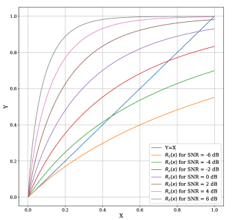
Figure 1: Functions $y=R_{c}(x)$ and $y=x$ for different values of $SNR=$ $10\log_{10}\left(c/4\right).$

Summarizing Lemmas 6-8, we have

Corollary 9.

Let $m\rightarrow\infty.$ Then r.v. $u_{i\,|\,\ell},$ $i=1,..,m,$ have power moments $x_{\ell}$ and $\sigma_{\ell}^{2}$ that satisfy equality $\left|x_{\ell}\right|=\sigma_{\ell}^{2}$ for any iteration $\ell.$ Iteration $\ell$ transforms $x_{\ell}$ and $\sigma_{\ell}^{2}$ into

$$\left|x_{\ell+1}\right|=\sigma_{\ell+1}^{2}=R_{c}(x_{\ell})$$ (45)

Proof of Theorem 4.

1. Lemma 8 shows that for $c>1,$ function $R_{c}(x_{\ell})$ grows for positive $x_{\ell}.$ Thus, equality $R_{c}(x_{\ell})=x_{\ell}$ holds iff $x_{\ell}=x_{\ast}$, where $x_{\ast}$ the root of (18). Next, consider initial iterations $\ell=0,...$ Here r.v. $u_{0}$ has pdf $\mathbb{N}(\delta,\delta/m)$ and (with high probability) has vanishing values $\left|u_{0}\right|\leq\sqrt{\delta/m}\ln m.$ In further iterations $\ell,$ transform (44) performs simple scaling $x_{\ell+1}\sim cx_{\ell}$ as long as $x_{\ell}\rightarrow 0$ for $m\rightarrow\infty.$ Thus, algorithm $\Psi_{soft}$ fails for $c<1$ since $x_{\ell}\rightarrow 0$ in this case.

2. Now let $c>1$ and $L=\ln m\,/\,\ln c.$ Note that $u_{0}<0$ with probability $Q(\sqrt{\delta m})\sim Q(\sqrt{c}).$ For iterations $\ell=o(L)$ and $m\rightarrow\infty,$ we still obtain vanishing moments $\left|E(u_{\ell})\right|\lesssim c^{\ell}\delta\rightarrow 0$ .It can also be verified that $E(u_{\ell})$ moves away from 0 in $\mu=\alpha L$ iterations for some $\alpha>0$.. Note also that r.v. $u_{\ell}$ has variance $\mathcal{D}(u_{\ell})\leq\mathcal{D}(u_{i\,|\,\ell})/m\leq 1/m.$ Thus, both cases, $u_{\ell}\rightarrow x_{\ast}$ or $u_{\ell}\rightarrow-x_{\ast},$ hold with high probability as $\ell\rightarrow\infty$.

3. We can now derive the BER for both cases. From (38) and (37), we see that the Gaussian random variable $h_{i\,|\,\ell+1}$ has the moments

$$E\left(h_{i\,|\,\ell+1}\right)\sim 2x_{\ell}E\left(Z_{i}\right)=2x_{\ell}c,\quad\mathcal{D}\left(h_{i\,|\,\ell+1}\right)\sim 4c\sigma_{\ell}^{2}$$

For any iteration $\ell,$ we can now estimate BER $p_{i\,|\,\ell+1}=\Pr\{h_{i\,|\,\ell+1}<0\}$ as

$$p_{i\,|\,\ell+1}=Q\left(x_{\ell}c/\sigma_{\ell}\sqrt{c}\right)=\left\{\begin{array}[c]{ll}Q\left(\sqrt{x_{\ell}c}\right),&\text{if}\;x_{\ell}>0\vskip 3.0pt plus 1.0pt minus 1.0pt\\ 1-Q\left(\sqrt{-x_{\ell}c}\right),&\text{if}\;x_{\ell}<0\end{array}\right.$$ (46)

4. Consider the probabilities $P_{\ell}=\Pr\left\{x_{\ell}<0\right\}$ and $1-P_{\ell}=\Pr\left\{x_{\ell}>0\right\},$ which define conditions of (46). We will now use two partial distributions of r.v. $u_{\ell}$ that have opposite means $\pm b_{\ell},$ where $b_{\ell}=|x_{\ell}|.$ According to (45), r.v. $u_{i\,|\,\ell}$ have the second moment $E(u_{i\,|\,\ell}^{2})=b_{\ell}.$ Then r.v. $u_{\ell}=\sum\nolimits_{i}\left(u_{i\,|\,\ell}/m\right)$ has the pdf $\mathbb{N}\mathcal{(}\pm b_{\ell},\eta_{\ell})$ with the variance

$$\eta_{\ell}=\left(b_{\ell}-x_{\ell}^{2}\right)/m=b_{\ell}(1-b_{\ell})/m$$

Note that $b_{\ell}\rightarrow x_{\ast}$ for $\ell>L,$ whereas $\eta_{\ell}\rightarrow 0$ as $\ell,m\rightarrow\infty.$ Thus, r.v. $u_{\ell}$ cross $0$ with a vanishing probability for any iteration $\ell>L.$ On the other hand, r.v. $u_{\ell}$ may cross 0 multiple times if $\ell=o(L).$ From now on, we take $\ell=o(L).$ Then we will express $P_{\ell+1}$ via $P_{\ell}$ using the mean

$$b_{\ell}=c^{\ell}\delta$$

5. Consider both distributions $\mathbb{N}\mathcal{(}x_{\ell},\eta_{\ell}),$ where $x_{\ell}=\pm b_{\ell}=\pm c^{\ell}\delta.$ Given some value $u$ of r.v. $u_{\ell},$ define r.v. $u_{\ell+1}\,|\,u=m^{-1}\sum\nolimits_{i}\left(u_{i\,|\,\ell+1}\,|\,u\right).$ This r.v. has pdf

$$p(u)=\mathbb{N}(cu,c\eta_{\ell})=(2\pi\eta_{\ell})^{-1/2}e^{-(u-x_{\ell})^{2}m/2\eta_{\ell}}$$

First, let $E(u_{\ell})=b_{\ell}.$ Clearly $\Pr\{cu<0\}=Q(u\sqrt{c/\eta_{\ell}}).$ Then we average over all values $u$ of $u_{\ell}$ and obtain the probability

$$S_{\ell} =\Pr\{u_{\ell+1}\,<0\,|\,E(u_{\ell})=b_{\ell}\}=\int_{-\infty}^{\infty}Q(u\sqrt{c/\eta_{\ell}})p(u)du$$

$$\sim(2\pi)^{-1/2}\int_{-\infty}^{\infty}Q(t\sqrt{c})e^{-(t-b_{\ell}/\sqrt{\eta_{\ell}})^{2}/2}dt$$

Here we use variable $t=u/\sqrt{\eta_{\ell}}.$ Next, we consider the initial iterations $\ell=o(\ln m/\ln c)$ and introduce parameter

$$C_{\ell}=b_{\ell}/\sqrt{\eta_{\ell}}\sim\sqrt{c^{\ell+1}/(1-m^{-1}c^{\ell+1})}\sim c^{\left(\ell+1\right)/2}$$ (47)

Note that $b_{\ell}/\sqrt{\eta_{\ell}}=C_{\ell}\sim c_{\ell},$ which gives (19). Similarly, for $E(u_{\ell})=-b_{\ell},$ we obtain the probability

$$Q_{\ell}=\Pr\{u_{\ell+1}<0\,|\,E(u_{\ell})=-b_{\ell}\}=\int_{-\infty}^{\infty}Q(u/\sqrt{c/\eta_{\ell}})p(-u)du$$

For $\ell<L=\ln m/\ln c,$ this gives the probability

$$P_{\ell+1}=\Pr\left\{u_{\ell+1}<0\right\}=\left(1-P_{\ell}\right)S_{\ell}+P_{\ell}Q_{\ell}=S_{\ell}+P_{\ell}T_{\ell}$$ (48)

where $T_{\ell}=Q_{\ell}-S_{\ell}$ is given by (20). We can also slightly tighten estimates (19) and (20), by using quantity $C_{\ell}$ of (47) instead of $c_{\ell}.$

We can now proceed with iterations $P_{\ell}$, which begin with $P_{0}=Q(\sqrt{c}).$ For any $\ell,$ quantities $S_{\ell}$ and $T_{\ell}$ depend on $c$ only. Also, quantities $c_{\ell}=c^{\left(\ell+1\right)/2}$ grow exponentially, in which case $S_{\ell}\rightarrow 0$ and $Q_{\ell}\rightarrow 1.$ Thus, quantities $P_{\ell}$ converge, since $P_{\ell+1}\sim P_{\ell}Q_{\ell}$ for sufficiently large $\ell\geq L.$

We can now evaluate $P_{soft}.$ For $\ell\rightarrow\infty,$ we replace $P_{\ell}$ with $P_{\infty}$ in (48) and use $x_{\ast}$ of (18). Finally, note that (21) is only an asymptotic estimate. Here we excluded the residual term $O\left(\ln m/\sqrt{m}\right)$ used in approximations (31) and (33). ${\blacksquare}$

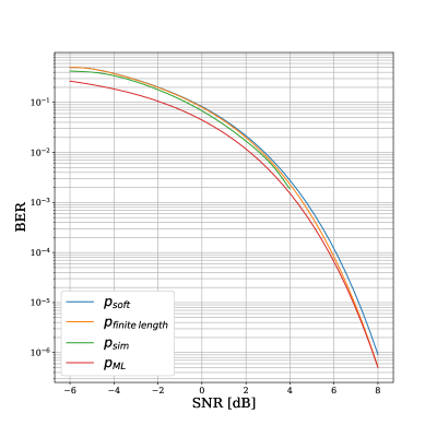
Figure 2: Simulation results and analytical bounds for the algorithm $\Psi_{soft}$ applied to modulation-type codes $C_{128}$ of length $8256.$

High-signal case. Consider functions $S_{\ell}$ and $T_{\ell}$ of (19) and (20) as $c\rightarrow\infty.$ Then $S_{\ell}\rightarrow 0,$ $T_{\ell}\rightarrow 1,$ and $P_{\infty}\rightarrow P_{0}=Q\left(\sqrt{c}\right).$ In this case, $P_{soft}\sim 2Q\left(\sqrt{c}\right)\sim(2/\pi c)^{1/2}e^{-c/2}.\$The latter represents a 3 dB gain over the uncoded modulation, whose BER has the order of $e^{-c/4}.$  

Complexity. Given $m$ information bits, algorithm $\Psi_{soft}$ has complexity of order $m^{2}\log m$. Indeed, each iteration $\ell$ recalculates quantities $u_{i\,|\,\ell}(j)$ and $h_{i\,|\,\ell}(j)$ for all ordered pairs $(i,j).$ This requires $O(m^{2})$ operations. We also need $O(\log m\,/\,\log c)$ iterations $\ell$ to make the estimates $u_{i\,|\,\ell}$ bounded away from 0 as $m\rightarrow\infty$. Also, it can be shown that the stable point $x_{\ast}$ can be reached within a margin $\varepsilon\rightarrow 0$ in $O\left(\ln\varepsilon^{-1}\,/\,\ln c\right)\,$ iterations. For $\varepsilon=m^{-1},$ this gives the overall complexity of $m^{2}\ln m\,/\,\ln c$ operations.

Simulation results vs analytical bounds. In Fig. 2, we plot analytical bound $P_{soft}$ of (21) along with simulation results $P_{sim}$ and the lower bound $P_{ML}$ of (9). Here we consider codes $C_{m}$ of dimension $m=128$ on the AWGN channels with various SNRs $10\log_{10}(c/4).$ We see that both bounds (21) and (9) tightly follow simulation results and each other. This also supports our main assumption that the algorithm $\Psi_{soft}$ can be considered using independent random variables. For completeness, we also plot non-asymptotic bound $P_{finite\;length}$ obtained by using parameters $C_{\ell}$ of (47) in both formulas (19) and (20). Unexpectedly, this bound completely coincides with a much simpler lower bound $P_{ML}$ for high SNR.

5 Multilevel protection schemes

Let $B_{i}=B_{i}(\mu,\mu r_{i}$) be a sequence of $b$ capacity-achieving polar codes. The rates $0\leq r_{0}<...<r_{b-1}$ will be specified later. We first encode data block $\overline{\mathbf{a}_{i}}$ of length $\mu r_{i}$ into some vector $A_{i}\in B_{i}$ and then form a compound block $A=\left(A_{0},...,A_{b-1}\right)$ of length $m=\mu b.$ Below $\mu\rightarrow\infty$ and $\ b$ is a constant. Block $A$ is further encoded by code $C_{m}$ of rate $R_{m}=2/(m+1)$ and length $n=\left({}_{2}^{m+1}\right).$ We use notation $\widehat{C}_{m}$ for the compound code of rate $R\sim R_{m}r,$ where $r=\sum\nolimits_{i}r_{i}/b.$ Thus, code $\widehat{C}_{m}$ reduces code rate $R_{m}$ by a factor of $r,$ which gives SNR of $c/4r$ per information bit.

Let $I_{s}=\{\mu s+1,...,\mu(s+1)\}$ for any $s=0,...,b-1.$ The received block $\widehat{C}=\widehat{C}(0)$ of length $n$ is first decoded by the algorithm $\Psi_{soft}$ using $L=O(\ln m)$ iterations. The result is some block $\widehat{A}(0)$ of length $m.$ We then retrieve the first $\mu$ decoded bits in $\widehat{A}(0)$ that form the sub-block $\widehat{A}_{0}=\left(\widehat{a}_{1},...,\widehat{a}_{\mu}\right)$ of length $\mu.$ Block $\widehat{A}_{0}$ is decoded by a polar code $B_{0}$ into some block $A_{0}=\{a_{1},...,$ $a_{\mu}\}.$ We assume that the corrected block $A_{0}$ has $WER\rightarrow 0$ as $\mu\rightarrow\infty$. We then use $A_{0}$ to replace the first $\mu$ symbols of the block $\widehat{C}(0)$. The result is a new block $\widehat{C}(1)$ of length $n.$ This completes round $s=0$.

Round $s=1$ is similar. Algorithm $\Psi_{soft}$ now also employs block $A_{0}$ to recalculate the remaining $m-\mu$ information bits of $\widehat{C}(1).$ The obtained sub-block $\widehat{A}_{1}=\left(\widehat{a}_{\mu+1},...,\widehat{a}_{2\mu}\right)$ is decoded into some vector $A_{1}=\{a_{\mu+1},...,$ $a_{2\mu}\}$ using code $B_{1}.$ Then $A_{1}$ replaces $\widehat{A}_{1}$ in positions $i\in I_{1}$ and yields a new block $\widehat{C}(2)$. Similarly, rounds $s=2,...,b-1$ only retrieve a block $A_{s}$ on positions $i\in I_{s}$ Then we obtain block $\widehat{C}(s+1)$ that include corrected bits $a_{1},...,$ $a_{\left(s+1\right)\mu}.$

In any round $s,$ $\mu s$ corrected information bits serve as frozen bits and aid the algorithm $\Psi_{soft}$. Indeed, with high probability, we use correct estimates $u_{j\,|\,\ell}=a_{j}$ for all $j\leq\mu s.$ Then the parity checks $u_{i\,|\,\ell+1}(j)=u_{i,j}u_{j\,|\,\ell}$ are reduced to the repetitions/inversions $u_{i\,|\,\ell+1}(j)=a_{j}u_{i,j}$ of symbols $u_{i,j}.$ Also, recall that algorithm (7) outputs the likelihoods $h_{i\,|\,L}$ of all symbols $a_{i}.$ Thus, we use $h_{i\,|\,L}$ as our bit estimates in every round $s$ as follows.

Let an information block $A$ consist of $m$ zeros. We then use antipodal signaling and transmit a codeword $1^{n}$ over an AWGN channel. Round $s$ includes $\mu s$ correct information bits $u_{i\,|\,\ell}=a_{i}=1.$ Let $\lambda_{s}=s/b.$ Then the remaining $m-\mu s$ r.v. $u_{i\,|\,\ell}$, $i>\mu s,$ have the average power moments 

$$x_{\ell} =\left[m\left(1-\lambda_{s}\right)\right]^{-1}\sum\nolimits_{i>\mu s}Eu_{i\,|\,\ell}$$ (49)

$$\sigma_{\ell}^{2} =\left[m\left(1-\lambda_{s}\right)\right]^{-1}\sum\nolimits_{i>\mu s}E\left(u_{i\,|\,\ell}^{2}\right)$$ (50)

In particular, the initial setup with $\ell=0$ employs the original r.v. $u_{i\,|\,0}$ that have asymptotic pdf $\mathbb{N}(\delta,\delta)$ for all $i>\mu s$ and satisfy equalities $x_{0}=\sigma_{0}^{2}=\delta.$

Theorem 10.

Let the algorithm $\Psi_{soft}$ have $\lambda m$ correct information symbols $a_{1}=...=a_{\lambda m}=1,$ where $\lambda\in(0,1).$ Then the remaining $(1-\lambda)m$ symbols $a_{i}$ have BER

$$P_{soft}(\lambda,c)\sim Q\left(\sqrt{cX(\lambda)}\right)$$ (51)

where $X(\lambda)$ satisfies equations

$$X(\lambda) =\lambda+\left(1-\lambda\right)x(\lambda)$$ (52)

$$x(\lambda) =\left(2\pi\right)^{-1/2}\int_{-\infty}^{\infty}\tanh\left(t\sqrt{cX(\lambda)}\right)e^{-\left(t-\sqrt{cX(\lambda)}\right)^{2}/2}dt$$ (53)

Proof. In essence, we follow the proof of Theorem 4. The main difference - that simplifies the current proof - is that the former vanishing point $x_{0}=\delta\rightarrow 0$ is now replaced with $X_{0}\rightarrow\lambda.\$ This removes the random walks across 0 analyzed in parts 4 and 5 of the former proof. Thus, now we have the case of $P_{\infty}=0.$ The details are as follows.

For any $j\geq\mu s+1,$ we use approximations (34) and (35) and take $u_{j\,|\,\ell}=1$ for $j\leq\mu s.$ Then

$$h_{i\,|\,\ell+1}(j)\sim 2u_{i\,|\,\ell+1}(j)\sim\left\{\begin{array}[c]{ll}z_{i,j}u_{j\,|\,\ell},&\text{if}\;j\geq\mu s+1\vskip 3.0pt plus 1.0pt minus 1.0pt\\ z_{i,j},&\text{if}\;j\leq\mu s\end{array}\right.$$

For any given $Z_{i},$ consider the sums $Z_{i}^{\prime}=\sum\nolimits_{j\leq\mu s}z_{i,j}$ and $Z_{i}^{\prime\prime}=\sum\nolimits_{j\geq\mu s+1}z_{i,j}.$ These sums have expected values $E(Z_{i}^{\prime})=\lambda Z_{i}$ and $E(Z_{i}^{\prime\prime})=\left(1-\lambda\right)Z_{i}.\$Let

$$X_{\ell} =\lambda+\left(1-\lambda\right)x_{\ell}$$

$$\theta_{\ell}^{2} =\lambda+\left(1-\lambda\right)\sigma_{\ell}^{2}$$

Then we define the moments

$$E\left(h_{i\,|\,\ell+1}\right)\sim 2x_{\ell}Z_{i}^{\prime\prime}+2Z_{i}^{\prime}\sim 2Z_{i}\left[\lambda+x_{\ell}\left(1-\lambda\right)\right]=2Z_{i}X_{\ell}$$ (54)

$$\mathcal{D}\left(h_{i\,|\,\ell+1}\right)\sim 4c\left(1-\lambda\right)\sigma_{\ell}^{2}+4c\lambda=4c\theta_{\ell}^{2}$$ (55)

Thus, r.v. $h_{i\,|\,\ell+1}/2$ has Gaussian pdf $\mathbb{N}(X_{\ell}c,\theta_{\ell}^{2}c).$

Next. consider r.v. $u_{i\,|\,\ell+1}\sim\tanh(h_{i\,|\,\ell+1}/2).$ Similarly to equalities (29) and (30), we have

$$E\left(u_{i\,|\,\ell+1}\right) \sim\left(2\pi\theta_{\ell}^{2}c\right)^{-1/2}\int_{-\infty}^{\infty}\tanh(z)e^{-\left(z-X_{\ell}c\right)^{2}/2c\theta_{\ell}^{2}}dz=F_{c}(X_{\ell},\theta_{\ell})$$ (56)

$$E[u_{i\,|\,\ell+1}^{2}] \sim\left(2\pi\theta_{\ell}^{2}c\right)^{-1/2}\int_{-\infty}^{\infty}\tanh^{2}(z)e^{-\left(z-X_{\ell}c\right)^{2}/2\theta_{\ell}^{2}c}dz=G_{c}(X_{\ell},\theta_{\ell})$$

Any round $s=\lambda b$ begins with the initial values $X_{0}(\lambda)$ and $\theta_{0}^{2}(\lambda)$ that satisfy equalities

$$X_{0}(\lambda)=\theta_{0}^{2}(\lambda)=\lambda+\delta\left(1-\lambda\right)\sim\lambda$$ (57)

which are similar to the former equality $x_{0}=\sigma_{0}^{2}$. Thus, we may follow the proof of Theorem 4 and obtain equality $F_{c}(X_{\ell},\theta_{\ell})=G_{c}(X_{\ell},\theta_{\ell})$ for any iteration $\ell.$ Now we see that $x_{\ell+1}=\sigma_{\ell+1}^{2}$ and $X_{\ell}=\theta_{\ell}^{2}$. Then for any $\lambda$ and $\ell\rightarrow\infty,$ we use variables $x(\lambda)$ and $X(\lambda)=\lambda+\left(1-\lambda\right)x(\lambda).$ Equalities (49) and (56) then give

$$x(\lambda)=E\left(u_{i}^{\infty}\right)=F_{c}(X(\lambda),\sqrt{X(\lambda)})$$

which can be rewritten as (53).

This also gives estimate (51). Indeed, iterations (54) and (55) show that the original iteration for $\ell=0$ gives r.v. $h_{i}^{1}$ that has Gaussian pdf $\mathbb{N}(2\lambda c,4\lambda c).$ Then for any round $s=\lambda b,$ r.v. $u_{1}=m^{-1}\sum\nolimits_{i>\mu s}$ $u_{i\,|\,1}$ has the mean $F_{c}(\lambda c,\lambda c)=R(\lambda c)$ and the vanishing variance $\mathcal{D=}R(\lambda c)/(1-\lambda)m,$ where $R_{c}(x)$ is defined in (42). Thus, for any $\lambda>0,$ our iterations begin with the crossover probability $P_{0}=\Pr\left\{u_{1}\leq 0\right\}\rightarrow 0$ as $m\rightarrow\infty$. The latter implies that $P_{\ell}\rightarrow 0$ for $\ell\rightarrow\infty,$ as defined in (48). In turn, we can remove $P_{\infty}=0$ from (21). Now we can use r.v. $h_{i\,|\,\ell+1}$that have pdf $\mathbb{N}(2X_{\ell}c,4X_{\ell}c),$ according to (54) and (55). For $\ell\rightarrow\infty,$ this gives (51) as

$$P_{soft}(\lambda,c)=\Pr\{h_{i\,|\,\infty}<0\}\sim Q\left(\sqrt{X(\lambda)c}\right)\mathit{\ }$$ (58)

${\blacksquare}$

The absence of random walks in our current setup also makes bound (51) very tight. This is shown in Fig. 3, where we plot analytical BER of (51) along with simulation results obtained for the algorithm $\Psi_{soft}(\lambda).$ Here we consider codes $C_{m}$ with $m=128$ and test various fractions of frozen bits $\lambda=s/m$ and different $S/N$ ratios $10\log_{10}(c/4).$

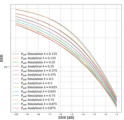
Figure 3: Simulation results and analytical bounds for the algorithm $\Psi_{soft}$ applied to modulation-type codes $C_{128}$ with a fraction $\lambda$ of frozen bits.

Recall that the likelihoods $h_{i\,|\,L}(\lambda)$ give BER (51) in round $s=\lambda b$. We can now represent any Gaussian r.v. $h_{i\,|\,L}(\lambda)$ as a channel symbol that has pdf $\mathbb{N(}1,\sigma^{2})$ and a BER $Q(1/\sigma).$ Thus, $\sigma^{2}=1/cX(\lambda).$ An important note is that codes $B_{s}(\mu,\mu r_{s})$ now operate on the AWGN channels $\mathbb{N(}0,\sigma^{2})$ that have a limited noise power $1/cX(\lambda).$ Unlike the original code $C_{m},$ we can now use codes $B_{s}(\mu,\mu r_{s})$ of non-vanishing code rates that grow from $r_{0}$ to $r_{b-1}.$

Theorem 11.

Codes $\widehat{C}_{m}$ of dimension $k\rightarrow\infty$ and length $n=O(k^{2})$ precoded with $b$ polar codes have overall complexity of $O(n\ln n).$ For sufficiently large $b,$ these codes achieve a vanishing BER if used arbitrarily close to the Shannon limit of $-1.5917$ dB per information bit.

Proof. In round $s=\lambda b,$ we use a capacity-achieving code $B_{s}(\mu,\mu r_{s}).$ The corresponding BI-AWGN channel $\mathbb{N}_{s}\mathbb{(}0,\sigma_{s}^{2})$ has noise power $\sigma_{s}^{2}=\left(X(\lambda)c\right)^{-1}$ and achieves capacity [14]

$$\rho_{c}(\lambda) =\log_{2}\sqrt{\frac{cX(\lambda)}{2\pi e}}-\int_{-\infty}^{\infty}f(y)\log_{2}f(y)\text{ }dy$$ (59)

$$f(y) =\sqrt{\frac{cX(\lambda)}{8\pi}}\left[e^{-(y+1)^{2}cX(\lambda)/2}+e^{-(y-1)^{2}cX(\lambda)/2}\right]$$

Here parameter $\lambda$ changes from 0 to 1 in small increments $1/b,$ which tend to $0$ as $b\rightarrow\infty.$ The average capacity for all AWGN channels $\mathbb{N}_{s}\mathbb{(}0,\sigma_{s}^{2})$ is $\rho_{c}=\int_{0}^{1}\rho_{c}(\lambda)d\lambda.$ Thus, for $m\rightarrow\infty,$ code $\widehat{C}_{m}$ achieves a vanishing BER for any code rate $r<2\rho_{c}/m,$ which gives $SNR>c/4\rho_{c}.$

We now proceed with code complexity. For $b$ polar codes $B_{s}(\mu,\mu r_{s}),$ design complexity has the order of $b\mu^{2}\sim 2n/b$ or less. Their decoding requires the order of $b\mu\ln\mu<m\ln m$ operations. Algorithm $\Psi_{soft}$ includes $b$ rounds with $L=O(\ln m)$ iterations in each round. This gives complexity order of $n\ln n$ if $b$ is a constant or $n\ln^{2}n$ for growing $b<\ln m.$ Thus, overall complexity has the order of $k^{2}\ln k,$ where $k\rightarrow\rho_{c}m$ is the number of information bits.

To calculate the minimum SNR $\varkappa=\min\nolimits_{c}\left(c/4\rho_{c}\right),$ we select parameters $c$ and $b.$ Then we solve equation (52) for different values of $\lambda=s/b,$ where $s=0,...,b-1$, and calculate $\rho_{c}$. The following table gives the highest value of code rate $\rho_{c},$ and the corresponding value of $\varkappa=\varkappa(c,b).$ Here we count $\varkappa$ in dB, as $10\log_{10}\varkappa$. The last line shows the gap $\varkappa/\ln 2-1$ to the Shannon limit of $\ln 2$.

$$b$$

(in dB)

    

Finally, note that $b$ is a constant for any $SNR>\ln 2.$ Statement 1 now follows directly from the existing bounds [12] on BER for polar codes. Here polar codes $B_{i}$ have length $\mu=m/b>2k/b.$ ${\blacksquare}$

6 Concluding remarks

In this paper, we study new codes that can approach the Shannon limit on the BI-AWGN channels. We first employ “modulation ” codes $C_{m}$ that use parity checks of weight 3. These codes can be aided by other codes $B_{m}$ via back-and-forth data recovery. Using BP algorithms that decode information bits only, codes $C_{m}$ achieve complexity order of $n\ln n$. Then new analytical techniques give tight lower and upper bounds on the output BER, which are almost identical to simulation results. Finally, we employ multilevel codes of dimension $k\rightarrow\infty$ that approach the Shannon limit with complexity order of $k^{2}$. One open problem is to find out if there exists a close-form solution to the transcendental equations (52), which (unexpectedly) give the Shannon limit using numerical integration in (59).

Our future goal is to improve code design for moderate lengths. This work in progress uses more advanced combinatorial designs for modulation codes. We conjecture that it also may reduce code complexity to the order of $\ln^{2}k$ operations per information bit for dimensions $k\rightarrow\infty.$

References

[1]G. D. Forney, Jr. and G. Ungerboeck, “Modulation and coding for linear Gaussian channels,” IEEE Trans. Info.
Theory, vol. 44, , pp. 2384-2415, Nov. 1998.
[2]R. Ratasuk, N. Mangalvedhe, Y. Zhang, M. Robert, and J.-P.
Koskinen, “Overview of narrowband IoT in LTE
Rel-13,” in Proc. IEEE Conf. Standard Commun. Netw., Berlin,
Germany, Oct./Nov. 2016, pp. 1–7.
[3]E. Abbe, A. Shpilka, and A. Wigderson, “ Reed-Muller Codes for Random Erasures and Errors,”IEEE Trans. Info. Theory, vol. 61, pp.5229-5252, Oct. 2015.
[4]R. Saptharishi, A. Shpilka and B.L. Volk,
“Efficiently decoding Reed-Muller codes from random
errors,” Proc. 48th Symp. Theory of Comp.
(STOC ’16), pp. 227-235, Cambridge, MA, USA, June 19, 2016.
[5]I. Dumer and K. Shabunov, “Near-optimum
decoding for subcodes of Reed-Muller codes,” 2001
IEEE Intern. Symp. Info. Theory, Washington DC, USA, June 24-29, 2001, p. 329.
[6] I. Dumer and K. Shabunov, “Soft
decision decoding of Reed-Muller codes: recursive lists,” IEEE Trans. Info. Theory, vol. 52, no. 3, pp. 1260-1266, 2006.
[7]V. Sidel’nikov and A. Pershakov, “Decoding
of Reed-Muller codes with a large number of errors,” Probl. Info. Transmission, vol. 28, no. 3, pp. 80-94, 1992.
[8]P. Loidreau and B. Sakkour, “Modified version
of Sidel’nikov-Pershakov decoding algorithm for binary second order
Reed-Muller codes,” Proc. 9th Intern.
Workshop on Algebraic and Combinatorial Coding theory, ACCT-9. Kranevo, 2004,
pp. 266–271.
[9]M. Ye and E. Abbe, “Recursive
projection-aggregation decoding of Reed-Muller codes”, Archive: 1902.01470v3
[cs.IT], 26 Feb. 2020.
[10]I. Dumer, “Polar codes with a stepped
boundary”, Proc. IEEE Intern. Symp. Info. Theory, Aachen, Germany, July
2017, pp. 2613-2617.
[11]M. Fereydounian, M.V. Jamali, H. Hassani, and H. Mahdavifar,
“Channel Coding at Low Capacity,” Proc. 2019 IEEE
Intern. Worshop. Info. Theory, Gotland, Sweden, August 2019, 5 pp.
[12]E. Arikan, “Channel polarization: A method for
constructing capacity-achieving codes for symmetric binary-input memoryless
channels,” IEEE Trans. Info. Theory, vol. 55 , pp.
3051-3073, July 2009.
[13]I. Dumer and N. Gharavi, “Codes for
high-noise memoryless channels,” 2020 Intern. Symp. Info. Theory and
Applications (Virtual Simposium), October 25-27, 2020, paper A03-04, pp. 101-105.
[14]T. M. Cover and J. A. Thomas, “Elements
of Information Theory,” 2nd edition, Wiley, Hoboken, NJ, 2006.