Shear Induced Orientational Ordering in Active Glass

Abstract

Dense assemblies of self propelled particles, also known as active or living glasses are abundant around us, covering different length and time scales: from the cytoplasm to tissues, from bacterial bio-films to vehicular traffic jams, from Janus colloids to animal herds. Being structurally disordered as well as strongly out of equilibrium, these systems show fascinating dynamical and mechanical properties. Using extensive molecular dynamics simulation and a number of different dynamical and mechanical order parameters we differentiate three dynamical steady states in a sheared model active glassy system: (a) a disordered phase, (b) a propulsion-induced ordered phase, and (c) a shear-induced ordered phase. We supplement these observations with an analytical theory based on an effective single particle Fokker-Planck description to rationalise the existence of the novel shear-induced orientational ordering behaviour in our model active glassy system that has no explicit aligning interactions, e.g. of Vicsek-type. This ordering phenomenon occurs in the large persistence time limit and is made possible only by the applied steady shear. Using a Fokker-Planck description we make testable predictions without any fit parameters for the joint distribution of single particle position and orientation. These predictions match well with the joint distribution measured from direct numerical simulation. Our results are of relevance for experiments exploring the rheological response of dense active colloids and jammed active granular matter systems.

Glassy or slow dynamics has been observed and thoroughly investigated in recent years in dense living or synthetic active matter systems across a range of scales, e.g. dense assemblies of cells Angelini et al. (2011), crowded cellular cytoplasm Parry et al. (2014), glassy liquids formed by self-propelled Janus colloids Klongvessa et al. (2019a, b) and jammed active granular solid Kumar et al. (2014); see Refs. Berthier et al. (2019); Janssen (2019) for recent reviews. Simulations and experiments have shown many non-trivial dynamical signatures, e.g. active jamming Henkes et al. (2011), shape dependent fluidization in a self-propelled Voronoi model Bi et al. (2015, 2016), glassy swirls in active dumbbells Mandal et al. (2017), intermittent dynamics with transient jamming Mandal et al. (2020), non-monotonic response in a glassy assembly of Janus colloidals Klongvessa et al. (2019a, b), along with the strong dynamical heterogeneity and slow density relaxation Berthier and Kurchan (2013); Ni et al. (2013); Berthier (2014) that are typical to passive supercooled liquids. Although dynamical aspects and transport in such active glassy systems have been looked at quite extensively, the response of such out-of-equilibrium systems to mechanical perturbation, i.e. their rheology, remains largely unexplored. Recently Barrat et. al. Matoz-Fernandez et al. (2017) have investigated the rheological response of a particular model dense active material that mimics the dynamics of tissue. In this model the number of particles is not conserved and particle death (apoptosis) and birth are modelled as a stochastic process.

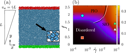
Figure 1: (a) Schematic of the active glass under steady shear, showing the upper wall (red particles) that moves steadily with velocity $v_{w}$, the static lower wall (green particles) and the bulk (blue particles); arrows represent the active forcing direction on each particle. (b) Phase diagram constructed from numerical MD simulation of the sheared active glass, showing different dynamical phases: (i) Disordered: orientationally disordered phase, (ii) PIO: propulsion-induced ordered phase and (iii) SIO: shear-induced ordered phase. The dashed blue line marks the boundary between the orientationally ordered and disordered phases; the solid black and dotted white lines delineate the separation between the PIO and the SIO phase according to two complimentary criteria (see text for details).

The authors of Matoz-Fernandez et al. (2017) observe a Newtonian crossover in the flow curves (stress versus strain rate) which is set by the cell death rate. In contrast to widely studied active particle classes (e.g. active Brownian particles (ABP) Fily and Marchetti (2012); Takatori and Brady (2015); Levis et al. (2017); Solon et al. (2018) or active Ornstein-Uhlenbeck particles Szamel (2014); Maggi et al. (2015)), the particles in Matoz-Fernandez et al. (2017) lack orientational degrees of freedom and active propulsion forces. The rheological response of active Brownian particles has also been explored Wagner et al. (2019) and an interesting velocity reversal phenomenon was observed near the boundary, though this study was limited to low-density suspensions of self propelled particles. Further studies exist of the shear response of active polar Giomi et al. (2010); Markovich et al. (2019) systems, again in the dilute regime, as well as nematic systems Muhuri et al. (2007); Cates et al. (2008) where liquid-crystalline ordering phenomena appear. But the overall understanding of the response to steady shear of active glassy systems made of isotropic particles with orientational degrees of freedom remains an open question in the literature.

In this article we report a new type of orientational ordering in a glassy assembly of active Brownian particles (ABP). This orientational order appears without any mutual alignment interaction between the particles (of e.g. Vicsek type Vicsek et al. (1995) or arising from anisotropic particle shapes) and is facilitated by shear. Using different physical quantities in steady shear, specifically (a) non-affinity in the velocity profile, (b) shear stress and (c) an orientational order parameter, we can differentiate between a number of qualitatively distinct steady states. Even though shear might naively be thought of as injecting additional fluctuations into the system and thus suppressing ordering, we find that it can in fact help the system to order orientationally. The three phases we observe are: (i) a disordered phase, (ii) a propulsion-induced ordered (PIO) phase, and (iii) a shear-induced ordered (SIO) phase. To understand the most intriguing state, which is the shear-induced ordered phase, we use a Fokker-Planck equation as an effective description of the single particle dynamics. Using a Galerkin truncation we evaluate the steady state joint probability distribution $P(\theta,y)$ of particle position (in the shear gradient direction) and orientation in closed form. The theoretically predicted distributions $P(\theta,y)$, for which all parameters can be determined independently, are in very good qualitative agreement with our simulation results in the shear-induced ordered phase.

Model

We study a model active glass Mandal et al. (2020); Mandal and Sollich (2020) that can be viewed as essentially a passive glass former but with the dynamics of each particle driven by a self-propulsion force in addition to the usual force from interaction with its neighbours. For the underlying passive glass former we use the well-known Kob-Andersen model Kob and Andersen (1995); Brüning et al. (2008), which is a $65:35$ binary mixture of soft particles with non-additive Lennard-Jones interactions. For their dynamics we assume an active Brownian particle form Fily and Marchetti (2012); Takatori and Brady (2015); Levis et al. (2017); Solon et al. (2018) (in terms of active forcing) with added steady shear:

$$m{\dot{\mathbf{v}}}_{i}=-\gamma(\mathbf{v}_{i}-\mathbf{v}_{F}(y_{i}))+\mathbf{F}_{i}+f\mathbf{n}_{i}.$$ (1)

Here $m$ is the mass of each particle and $\gamma$ the friction coefficient; we set both to $1$ in our study. We denote by $\mathbf{v}_{i}$ the velocity of the $i$-th particle and by $\mathbf{v}_{F}(y_{i})$ the local affine flow velocity from the applied shear; viscous damping is taken as relative to this flow and can thus be viewed as resulting from an affinely sheared solvent. With an imposed shear rate $\dot{\gamma}$ the affine velocity field is $\mathbf{v}_{F}(y)=\dot{\gamma}y\hat{\bf{e}}_{x}$ if $y$ denotes the position coordinate along the shear gradient direction and $\hat{\bf{e}}_{x}$ is the unit vector in the shear ($x$-)direction. To implement the constant shear rate we move all the particles in an upper wall with a constant velocity $v_{w}$ while the particles in the corresponding lower wall are static. The upper wall velocity then sets the imposed shear rate through the relation $\dot{\gamma}={v_{w}}/{L}$ where $L$ is the distance between the upper and lower walls; see the illustration in Fig. 1(a). We return below to the importance of implementing the steady shear with explicit walls.

Returning to the remaining terms in (1), ${\bf{F}}_{i}$ is the total force on particle $i$ resulting from the Kob-Andersen LJ interactions Kob and Andersen (1995); Brüning et al. (2008). The active force has constant magnitude $f$ and direction $\mathbf{n}_{i}=(\cos\theta_{i},\sin\theta_{i})$ for the $i$-th particle. Each angle $\theta_{i}$ changes diffusively, $\dot{\theta}_{i}=(2/\tau_{p})^{1/2}\eta_{i}(t)$ with $\eta_{i}(t)$ unit variance white noise; $\tau_{p}$ is thus the persistence time of the active forcing Mandal et al. (2020); Mandal and Sollich (2020).

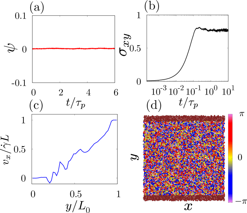
Figure 2: Disordered phase (marked by red square in phase diagram in Fig. 1(b)): (a) Orientational order parameter $\psi$ (see text for details) shows no emergent order in steady state. (b) Shear stress $\sigma_{xy}$ exhibits initial growth during startup of steady shear, with fluctuations around a finite value in steady state. (c) Instantaneous velocity profile (see Subsection: Material and Methods for details) in steady state is essentially linear with small non-affine fluctuations. (d) Snapshot of the system in the steady state shows uniform distribution of particle orientation $\theta$ as shown by colour bar.

Following the approach in Ref. Mandal et al. (2020); Mandal and Sollich (2020) we keep number density high ($\rho=1.2$) and focus mainly on the athermal limit ($T=0$). We will see later, however, that for small persistence times, $\tau_{p}=O(1)$, the active system can be mapped to an equivalent passive thermal system. Note also that while our the equation of motion does contain an inertial term, the value of friction coefficient ($\gamma=1$) that we use ensures that the dynamics is mostly overdamped Warren and Rottler (2013). We focus mostly on the two extreme limits of very small and very large persistence time $\tau_{p}$, choosing specifically $\tau_{p}=1$ and $\tau_{p}=10^{3}$. The key parameters for the phase diagrams we construct in this study are then the magnitude $f$ of the self-propulsion force and the imposed shear rate $\dot{\gamma}$.

Results

Small Persistence Time

We first performed steady shear simulations in the small persistence time limit ($\tau_{p}=1$) of our model active glass. In this regime the behaviour can be understood using the idea of an effective temperature generated by the rapidly fluctuating active forcing. We measured the steady state shear stress $\langle\sigma_{xy}\rangle$ for different applied shear rates $\dot{\gamma}$ and compared the flow curve of the active glass with $\tau_{p}=1$ and $f=0.7$ to the flow curve of the corresponding passive system ($f=0$) at an equivalent effective temperature $T_{\rm eff}=0.1$. These two sets of flow curves match very well (as shown in supplementary figure Fig. S1(b); see also SI for further discussion of the effective temperature). Indeed, from the time correlations of the active forces one expects $T_{\rm eff}$ to scale as $\tau_{p}f^{2}$ and this effective temperature description generally works well for active glasses in the small persistence time limit Mandal et al. (2020); Mandal and Sollich (2020). For most of the stress measurements in this study we use the virial stress, defined as $\sigma_{\alpha\beta}=-V^{-1}\sum^{N}_{i=1}r^{\alpha}_{i}F^{\beta}_{i}$ where $\mathbf{r}_{i}$ is the position of the $i$-th bulk particle, $\mathbf{F}_{i}$ is the total interaction force on this particle and $V$ is the volume of the bulk and $N$ is the number of particles in the bulk. We have also looked at the active stress defined as $\sigma^{a}_{\alpha\beta}=-V^{-1}\sum^{N}_{i=1}r^{\alpha}_{i}f^{\beta}_{i}$ where $\mathbf{f}_{i}=f\mathbf{n}_{i}$ is the active force acting on particle $i$. We observe that it fluctuates around zero (see supplementary Fig. S1(c)) and so can be ignored in the average stress; its fluctuation amplitude depends strongly on the active force magnitude ($f$) but only very weakly on the shear rate ($\dot{\gamma}$), see supplementary Fig. S1(c). As we are dealing with an active system, where the definition and meaning of stress has been much discussed, we also checked whether the virial stress calculated from the bulk matches with the direct measurement of stress from the forces on the walls. We see good agreement between the two approaches, both in a plot of stress versus strain as shear is started up at fixed shear rate, and in the flow curve ($\langle\sigma_{xy}\rangle$ versus $\dot{\gamma}$). We refer to the supplementary material for further discussion of the different stress definitions and their comparison (see in particular supplementary Fig. S2).

Large Persistence Time

We observe the physically most interesting behaviour for large values of the persistence time, in particular with regards to spatial ordering of the orientation of the active particles (as given by the direction of their propulsive force). We therefore now fix the persistence time to the large value $\tau_{p}=10^{3}$ and vary active forcing $f$ and shear rate $\dot{\gamma}$ within a broad range of values $f=\{0,2.6\}$, $\dot{\gamma}=\{10^{-4},10^{-1}\}$. We find three type of dynamical phases (see Fig. 1(b)): (a) disordered, (b) propulsion-induced ordered (PIO) and (c) shear-induced ordered (SIO). To differentiate these phases we use firstly an orientational order parameter. This is determined from the joint distribution $P(\theta,y)$ of the $y$-coordinates and orientations $\theta$ of the bulk particles as

$$\psi=\int_{-L/2}^{L/2}P(y)\phi(y)\sin{\left(\frac{2\pi y}{L}\right)}dy.$$ (2)

Here $\phi(y)$ is in turn defined as

$$\phi(y)=\frac{\int^{\pi}_{-\pi}P(\theta,y)\sin{\theta}\,d\theta}{P(y)},\quad P(y)=\int^{\pi}_{-\pi}P(\theta,y)d\theta.$$ (3)

Intuitively, $\phi(y)$ measures the dominant non-uniformity in the orientation distribution as a function of $y$ and is positive if particles point primarily towards the upper wall ($\theta\approx\pi/2$), and negative in the opposite case. The global order parameter $\psi$ thus detects whether the preferred particle orientation varies significantly in space, such that particles in the upper half of the system tend to point to the upper wall while those in the lower half point in the opposite direction. Both $\phi(y)$ and $\psi$ vanish for a uniform orientational distribution, $P(\theta,y)=P(y)/(2\pi)$. The colour bar in the phase diagram (see Fig. 1(b)) in the $(\dot{\gamma},f)$-plane shows the average value of the orientational order parameter $\psi$ in the steady state; the blue line is the contour for a small constant $\psi$ (we choose $\psi=0.05$) and so marks the boundary between orientationally ordered and disordered phases.

The black solid line and the white dashed line together mark the boundary between PIO and SIO, according to two complimentary criteria. The black solid line was calculated from the average stress and separates the regions of small and large stresses by a contour of constant $\langle\sigma_{xy}\rangle=0.4$ (roughly halfway between the typical values $\ll 1$ for PIO and $\approx 1$ for SIO). The white dashed line was determined from the strength of velocity fluctuations away from the affine flow field; it thus marks the boundary between phases with dominantly affine flow and those with significantly non-affine flow. In particular, we measure the average velocity in the shear direction $\langle v_{x}(y)\rangle$ as a function of $y$ and define $v^{\rm NA}$ as the root-mean-squared deviation of this (see Materials and Methods for definition) from the affine flow velocity $v_{Fx}(y)$. The white dashed line in Fig. 1(b) is then the contour ${v^{\rm NA}}/{v_{w}}=0.2$, where we use the upper wall velocity $v_{w}=\dot{\gamma}L$ as a natural velocity scale for the affine flow.

In the disordered phase the system behaves like a typical supercooled or glassy solid with Herschel-Bulkley rheology and a nonzero yield stress, around which stress fluctuations are seen in the steady state (see Fig. 2(b)). The particle orientations do not show any ordering (see Fig. 2(a) and the steady state snapshot in Fig. 2(d)) as $P(\theta,y)/P(y)$ remains close to ${1}/{2\pi}$. The velocity profile remains linear with almost negligible non-affine fluctuations (see Fig. 2(c)). These small non-affine fluctuations increase with the active forcing $f$ but decrease with increasing shear rate $\dot{\gamma}$ (data not shown). These trends can be seen as the precursors of respectively the PIO phase, which appears at larger $f$ and exhibits significantly non-affine velocities as we discuss next, and the SIO phase at larger $\dot{\gamma}$ with its essentially affine flow.

Upon increasing $f$ at small shear rate $\dot{\gamma}$ one enters the propulsion-induced ordered phase. This is characterized by a moderate amount of orientational ordering (see Fig. 3(a,d)) but strong non-affine flows created by the “stirring” arising from the strong active forces (see Fig. 3(c)). The system also shows significant density inhomogeneities ranging up to the formation of transient cavities (see supplementary movie) that remodel dynamically. The spatial segregation into dense regions and cavities with almost zero density can be thought of as an inverted type of motility-induced phase separation (MIPS) Tjhung et al. (2018); Shi et al. (2020); Caporusso et al. (2020). Because of this dynamic cavity formation and strong internal flows during the steady shear, the system is unable to sustain any significant shear stress in the steady state: the average stress reaches very low values, with strong fluctuations around the mean (see Fig. 3(b)). We call this phase “propulsion-induced ordered” because the spatial segregation is observable even for $\dot{\gamma}\to 0$, where the motion of the particles and hence the overall physics is dominated by the active propulsion forces.

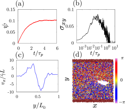
Figure 3: Propulsion-induced ordered phase (cyan circle in phase diagram in Fig. 1(b)): (a) Orientational order parameter $\psi$ shows growth during startup of steady shear, with saturation for $t\approx\tau_{p}$. (b) Shear stress $\sigma_{xy}$ fluctuates around zero in the steady state. (c) Instantaneous velocity profile in steady state demonstrates very strong non-affine fluctuations. (d) Snapshot of the system shows weak orientational order (see colour bar) and strong density inhomogeneities including transient cavity formation.

We next consider the shear-induced ordered phase. This can also be entered from the disordered phase, but along a different route: starting at moderate active forcing, $f\sim 1$, in the disordered phase one increases the shear rate $\dot{\gamma}$ from a very low value $\sim 10^{-3}$ to a quite substantial rate $\sim 10^{-1}$. The resulting SIO phase shows liquid-like properties in many respects. For example, it has an almost linear velocity profile with negligible non-affine fluctuations (see Fig. 4(c)). The shear stress increases after shear startup and reaches a constant steady state value on time scales around or above $\tau_{p}$ (see Fig. 4(b)). Surprisingly, however, these liquid-like features are combined with strong spatial order in the particle orientations (see Fig. 4(a,d)).

Summarizing our findings for the properties of the two ordered phases, PIO and SIO, these differ substantially in the spatial uniformity of the number density, in the presence or absence of non-affine flow and in their capability to support significant shear stress. The PIO phase is dominated by the physics of phase segregation, and shear does not play a significant role in its formation or stability. The SIO phase, on the other hand, exists only at reasonably large shear rates and active propulsion does not on its own guarantee the existence or stability of such a phase.

We next show that the qualitative behaviour of the SIO phase as an affinely flowing yet orientally ordered state can be understood by a simple analytical approach. This is based on an effective Fokker-Planck description of the single particle dynamics and will allows us to make quantitative predictions that can be verified by our simulations.

Effective single particle description

The dynamics of our model glass can in principle be described by a Fokker-Planck equation for the $3N$ particle coordinates and orientations $(x_{i},y_{i},\theta_{i})$, together with the associated momenta and supplemented by terms describing the wall motion. As the qualitative physics we are describing corresponds to an overdamped limit, the momenta can be ignored to a good approximation. The equation of motion for a single particle can then formally be derived by integrating out all other degrees of freedom Zwanzig (2001). We neglect the memory effects that generically occur in such a reduction (see e.g. Rubin et al. (2014); Herrera-Delgado et al. (2020)) and write an approximate Fokker-Planck equation for the joint distribution $P(\theta,y)$ of the orientation $\theta$ and $y$-position of a single particle:

$$\frac{\partial P(\theta,y)}{\partial t}+\mu f\sin{\theta}\frac{\partial P(\theta,y)}{\partial y}=D\frac{\partial^{2}P(\theta,y)}{\partial y^{2}}+D_{\theta}\frac{\partial^{2}P(\theta,y)}{\partial\theta^{2}}$$ (4)

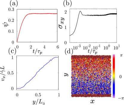
Figure 4: Shear Induced Ordered phase (marked by green triangle in phase diagram in Fig. 1(b)): (a) Orientational order parameter $\psi$ indicates a strongly ordered steady state. (b) Shear stress remains finite in steady shear, reaching a constant value at $t\approx\tau_{p}$. (c) Instantaneous velocity profile at steady state shows linear velocity profile with negligible non-affine fluctuations. (d) Snapshot of the system shows strong orientational order (see colour bar) but essentially homogeneous density.

Here $\mu$ is the effective mobility, $f$ is the active force magnitude as before, $D$ is the effective diffusion constant and $D_{\theta}=1/\tau_{p}$ is the orientational diffusion constant. The second term on the left hand side represents advection of probability due to active forcing, with the average $y$-velocity of the particle being proportional to the $y$-component $f\sin\theta$ of the active force. The terms on the right hand side describe translational and rotational diffusion, respectively. Our aim is now to obtain the steady state solution $P(\theta,y)$, from which predictions for the orientational order parameter can be derived according to (2) and (3). A Fourier decomposition of the angular dependence gives

$$P(\theta,y)=\sum_{m=-\infty}^{\infty}e^{im\theta}P_{m}(y)$$ (5)

where $P_{m}(y)$ is the $y$-dependent coefficient of the $m$-th Fourier mode. Substituting the representation (5) into (4) we obtain a system of coupled equations for the $P_{m}(y)$:

$$\frac{\mu f}{2i}\left[\frac{\partial P_{m-1}(y)}{\partial y}-\frac{\partial P_{m+1}(y)}{\partial y}\right]=D\frac{\partial^{2}P_{m}(y)}{\partial y^{2}}-m^{2}D_{\theta}P_{m}(y).$$ (6)

To find a closed form approximation for $P(\theta,y)$ we use a Galerkin truncation Fletcher (1984); specifically we truncate the series in (5) after the leading terms with $m=0,\pm 1$. We have checked that the inclusion of higher modes does not change the predictions qualitatively (see supplementary Fig. S3(a,b)). The boundary conditions required to fix the solution for $P(\theta,y)$ arise from the fact that the upper and lower walls in our system are impermeable so that the probability current in the $y$-direction, which is given by

$$J_{y}=(\mu f\sin{\theta})P-D\frac{\partial P}{\partial y}$$ (7)

has to vanish there:

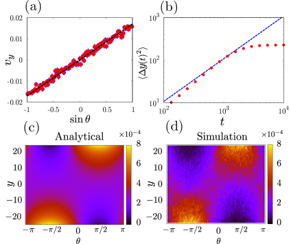
Figure 5: Single particle parameters in SIO phase marked in Fig. 1(b) (open triangle) (a) Average velocity of particles around $y=0$ in shear gradient ($y$) direction, plotted against $\sin\theta$, giving a linear relation as assumed in our single particle theory; the slope identifies the mobility $\mu$. (b) Mean-squared displacement of particles starting around $y=0$ (marked by red points) and a linear fit (blue dashed line) to extract $D_{m}$. (c,d) Comparison of steady state $P(\theta,y)$ from the analytical single particle theory and from simulation, showing good agreement without fit parameters.

$$J_{y}=\begin{cases}0,&\text{at }y=-L/2\\ 0,&\text{at }y=+L/2\end{cases}$$ (8)

Away from the walls we find that $J_{y}$ is generically nonzero, reflecting the non-equilibrium character of the system. The full current vector $(J_{\theta},J_{y})$ exhibits interesting structure, with the corresponding flow splitting the $(\theta,y)$-plane into a number of distinct regions as shown in supplementary Fig. S3(c). With the above boundary conditions we find the steady state solution for the dominant Fourier modes as

$$P_{0}(y)=\frac{1}{2\pi}\frac{\cosh(\alpha y)+\zeta\cosh(\alpha L/2)}{\zeta L\cosh(\alpha L/2)+\frac{2}{\alpha}\sinh(\alpha L/2)}\ ,$$ (9)

and

$$P_{1}(y)=-i\frac{\alpha D}{\mu f}\frac{1}{2\pi}\frac{\sinh(\alpha y)}{\zeta L\cosh(\alpha L/2)+\frac{2}{\alpha}\sinh(\alpha L/2)}$$ (10)

with $P_{-1}(y)=-P_{1}(y)$. Here the inverse length scale $\alpha$ is defined via $\alpha^{2}=(\mu^{2}f^{2}+2DD_{\theta})/(2D^{2})$. Inserting into the Fourier expansion of (5) with our Galerkin truncation

$$P(\theta,y)=e^{i\theta}P_{1}(y)+e^{-i\theta}P_{-1}(y)+P_{0}(y)$$ (11)

gives the desired steady state joint distribution

$$\begin{split}P(\theta,y)=&\frac{\alpha D}{\mu f}\ \frac{2\sin{\theta}\sinh(\alpha y)}{2\pi(\zeta L\cosh(\alpha L/2)+\frac{2}{\alpha}\sinh(\alpha L/2))}\\ &{}+{}\frac{\cosh(\alpha y)+\zeta\cosh(\alpha L/2)}{2\pi(\zeta L\cosh(\alpha L/2)+\frac{2}{\alpha}\sinh(\alpha L/2))}\end{split}$$ (12)

From this we can finally deduce the local orientational order parameter $\phi(y)$ defined in (3):

$$\phi(y)=\frac{\alpha D}{\mu f}\frac{\sinh(\alpha y)}{\cosh(\alpha y)+\zeta\cosh(\alpha L/2)}$$ (13)

To assess these theoretical predictions we can take most parameters directly from simulations and use for a typical SIO phase $f=1$, $\tau_{p}=10^{3}$ and $L_{0}=50$. The remaining two effective single particle parameters can be measured directly from the simulation (see Fig. 5(a,b)): the mobility $\mu=v_{y}/(f\sin{\theta})$ can be extracted from the relation between the average velocity of the particles and their orientation and the diffusion constant from $D_{m}=\langle{\Delta y(t)}^{2}\rangle/(2t)$ (see Material and Methods). As the diffusive description is approximate (see below) we take a somewhat larger $D$ in the theory, $D=3.3D_{m}$. With $\mu$ and $D$ fixed independently, there are no remaining free parameters in the theory. Fig. 5(c,d) shows the comparison of the theoretically predicted $P(\theta,y)$ and the steady state simulation data in the corresponding SIO phase. We observe very good qualitative and semi-quantitative agreement, particularly given the approximations inherent in the theory: (i) the simulations show a super-diffusive growth of the mean-squared particle displacement, suggesting that memory effects cannot be fully neglected as we have done; (ii) the effective diffusivity $D$ and mobility $\mu$ may exhibit some dependence on density and therefore $y$, whereas we have taken these parameters as constant. Overall, our simple single particle theory offers a remarkably good description of the SIO phase and its orientational ordering. Within the theoretical picture the degree of orientational ordering is governed by the competition between the orientational bias of the particle velocities in the shear gradient direction on the one hand, and the disordering tendency of the rotational diffusion on the other. Ordering is observable when the steady shear leads to a sufficiently large effective mobility and hence a stronger tendency towards orientational order.

Discussion

In this work we explored the effect of steady shear deformation in a model active glassy material and report a new type of orientational ordering that is facilitated by shear. Using different physical quantities including non-affinity in the velocity profile, steady state shear stress and an orientational order parameter, we were able to distinguish a number of qualitatively distinct dynamical steady states: (i) a disordered phase, (ii) a propulsion-induced ordered phase and (iii) a shear induced-ordered phase. We observe in particular that shear can help the system to order orientationally, effectively by mobilizing particles sufficiently to follow their orientational bias. For the SIO phase, which exhibits strong orientational ordering yet essentially affine flow, we constructed a single particle Fokker-Planck theory that predicts the joint steady state distribution $P(\theta,y)$ and hence the degree of orientational order in the system. The predictions compare well with simulation data. There are no free fit parameters in this comparison as the two required effective single particle quantities (mobility and diffusion constant) can be measured directly in the simulations.

Shear-induced phase transitions and ordering phenomena in passive systems have been an active topic of research for some time Ackerson and Pusey (1988); Ackerson (1990); Stevens and Robbins (1993); Wu et al. (2009). It has been shown that although shear can destroy order by melting a system Stevens and Robbins (1993), it can also induce ordering in the sense of crystallisation Ackerson and Pusey (1988); Stevens and Robbins (1993); Wu et al. (2009); Khabaz et al. (2017); Ruiz-Franco et al. (2018) or alignment for elongated particles Koppi et al. (1993); Börzsönyi et al. (2012). Shear-induced crystallization has also been reported very recently in passive colloidal Janus particles Huang et al. (2019). Our results demonstrate that new forms of shear-induced ordering can arise in active systems, which are inherently out of equilibrium even without shear. This will add new directions to the exciting paradigm of ordering through steady shear driving.

It will be an interesting challenge to see whether our theoretical approach can be extended into a complete theory for all phases we see, including a prediction of the phase boundaries. This would require in particular accounting appropriately with the spatial inhomogeneities of the PIO phase. Another interesting direction would be to study shear ordering in chiral active systems, where qualitatively new phenomena might be expected. The novel orientational ordering we have found can also be explored and exploited in synthetic active glassy systems, in controlled experiments on active colloids or active granular matter.

Materials and Methods

The simulations were performed in two spatial dimensions with a square box with periodic boundary condition implemented along the direction of flow. We used modified Langevin dynamics Beard and Schlick (2000) for the MD simulation with $dt=0.002$. We averaged all steady state quantities over a time scale of $t=10^{4}$ after first allowing the same amount of time for the system to reach a steady state. This is ample as for our largest $\tau_{p}=10^{3}$ the relaxation to the steady state still happens on a timescale of order $\tau_{p}$. Apart from this temporal averaging, the order parameter $\psi$, shear stress $\sigma_{xy}$, and other relevant quantities are also averaged over $128$ independent simulations. We compared simulations with $N_{0}=1000$ and $N_{0}=4000$ particles to check for finite size effects; all results shown were generated for $N_{0}=4000$. Here $N_{0}$ includes both the bulk and boundary (wall) particles. This corresponds to a box size of $L_{0}=57.73$ (as number density is $\rho=1.2$) with a distance between the two walls of $L=50$ and an wall thickness of approximately $4\sigma_{AA}$. Velocity profiles are calculated by dividing the whole system into $N_{s}=50$ slabs in the $y$-direction. For the calculation of $v^{NA}$ we average the mean square fluctuations around the affine velocity $v_{Fx}(y)$ across $y$-bins and evaluate the root of this mean squared fluctuation. This means that for $N_{0}=4000$, averages within a slab are taken over $80$ particles on average. To determine the measured effective diffusion constant $D_{m}$ we divided the system into $5$ slabs and measured $\langle(\Delta{y(t)})^{2}\rangle$ in each of them. The diffusion constant was then determined from $\langle(\Delta y(t))^{2}\rangle/(2t)$ at the time $t$ where $\langle(\Delta y(t))^{2}\rangle^{1/2}\sim 10$, which is the size of each slab in the $y$-direction.

We are grateful to Jörg Rottler and Rohit Jain for insightful discussions. This project has received funding from the European Union’s Horizon 2020 research and innovation programme under Marie Skłodowska-Curie grant agreement No. 893128.

References

- Angelini et al. (2011) T. E. Angelini, E. Hannezo, X. Trepat, M. Marquez, J. J. Fredberg, and D. A. Weitz, Proceedings of the National Academy of Sciences 108, 4714 (2011), https://www.pnas.org/content/108/12/4714.full.pdf .
- Parry et al. (2014) B. Parry, I. Surovtsev, M. Cabeen, C. O’Hern, E. Dufresne, and C. Jacobs-Wagner, Cell 156, 183 (2014).
- Klongvessa et al. (2019a) N. Klongvessa, F. Ginot, C. Ybert, C. Cottin-Bizonne, and M. Leocmach, Phys. Rev. Lett. 123, 248004 (2019a).
- Klongvessa et al. (2019b) N. Klongvessa, F. Ginot, C. Ybert, C. Cottin-Bizonne, and M. Leocmach, Phys. Rev. E 100, 062603 (2019b).
- Kumar et al. (2014) N. Kumar, H. Soni, S. Ramaswamy, and A. Sood, Nature communications 5, 1 (2014).
- Berthier et al. (2019) L. Berthier, E. Flenner, and G. Szamel, The Journal of Chemical Physics 150, 200901 (2019), https://doi.org/10.1063/1.5093240 .
- Janssen (2019) L. M. C. Janssen, Journal of Physics: Condensed Matter 31, 503002 (2019).
- Henkes et al. (2011) S. Henkes, Y. Fily, and M. C. Marchetti, Phys. Rev. E 84, 040301 (2011).
- Bi et al. (2015) D. Bi, J. Lopez, J. M. Schwarz, and M. L. Manning, Nature Physics 11, 1074 (2015).
- Bi et al. (2016) D. Bi, X. Yang, M. C. Marchetti, and M. L. Manning, Phys. Rev. X 6, 021011 (2016).
- Mandal et al. (2017) R. Mandal, P. J. Bhuyan, P. Chaudhuri, M. Rao, and C. Dasgupta, Phys. Rev. E 96, 042605 (2017).
- Mandal et al. (2020) R. Mandal, P. J. Bhuyan, P. Chaudhuri, C. Dasgupta, and M. Rao, Nature communications 11, 1 (2020).
- Berthier and Kurchan (2013) L. Berthier and J. Kurchan, Nature Physics 9, 310 (2013).
- Ni et al. (2013) R. Ni, M. A. C. Stuart, and M. Dijkstra, Nature communications 4, 1 (2013).
- Berthier (2014) L. Berthier, Phys. Rev. Lett. 112, 220602 (2014).
- Matoz-Fernandez et al. (2017) D. A. Matoz-Fernandez, E. Agoritsas, J.-L. Barrat, E. Bertin, and K. Martens, Phys. Rev. Lett. 118, 158105 (2017).
- Fily and Marchetti (2012) Y. Fily and M. C. Marchetti, Phys. Rev. Lett. 108, 235702 (2012).
- Takatori and Brady (2015) S. C. Takatori and J. F. Brady, Physical Review E 91, 032117 (2015).
- Levis et al. (2017) D. Levis, J. Codina, and I. Pagonabarraga, Soft Matter 13, 8113 (2017).
- Solon et al. (2018) A. P. Solon, J. Stenhammar, M. E. Cates, Y. Kafri, and J. Tailleur, New Journal of Physics 20, 075001 (2018).
- Szamel (2014) G. Szamel, Phys. Rev. E 90, 012111 (2014).
- Maggi et al. (2015) C. Maggi, U. M. B. Marconi, N. Gnan, and R. Di Leonardo, Scientific reports 5, 10742 (2015).
- Wagner et al. (2019) C. G. Wagner, M. F. Hagan, and A. Baskaran, Phys. Rev. E 100, 042610 (2019).
- Giomi et al. (2010) L. Giomi, T. B. Liverpool, and M. C. Marchetti, Phys. Rev. E 81, 051908 (2010).
- Markovich et al. (2019) T. Markovich, E. Tjhung, and M. E. Cates, Phys. Rev. Lett. 122, 088004 (2019).
- Muhuri et al. (2007) S. Muhuri, M. Rao, and S. Ramaswamy, Europhysics Letters (EPL) 78, 48002 (2007).
- Cates et al. (2008) M. E. Cates, S. M. Fielding, D. Marenduzzo, E. Orlandini, and J. M. Yeomans, Phys. Rev. Lett. 101, 068102 (2008).
- Vicsek et al. (1995) T. Vicsek, A. Czirók, E. Ben-Jacob, I. Cohen, and O. Shochet, Phys. Rev. Lett. 75, 1226 (1995).
- Mandal and Sollich (2020) R. Mandal and P. Sollich, Phys. Rev. Lett. 125, 218001 (2020).
- Kob and Andersen (1995) W. Kob and H. C. Andersen, Phys. Rev. E 51, 4626 (1995).
- Brüning et al. (2008) R. Brüning, D. A. St-Onge, S. Patterson, and W. Kob, Journal of Physics: Condensed Matter 21, 035117 (2008).
- Warren and Rottler (2013) M. Warren and J. Rottler, Phys. Rev. Lett. 110, 025501 (2013).
- Tjhung et al. (2018) E. Tjhung, C. Nardini, and M. E. Cates, Phys. Rev. X 8, 031080 (2018).
- Shi et al. (2020) X.-q. Shi, G. Fausti, H. Chaté, C. Nardini, and A. Solon, Phys. Rev. Lett. 125, 168001 (2020).
- Caporusso et al. (2020) C. B. Caporusso, P. Digregorio, D. Levis, L. F. Cugliandolo, and G. Gonnella, Phys. Rev. Lett. 125, 178004 (2020).
- Zwanzig (2001) R. Zwanzig, Nonequilibrium statistical mechanics (Oxford University Press, 2001).
- Rubin et al. (2014) K. J. Rubin, K. Lawler, P. Sollich, and T. Ng, Journal of Theoretical Biology 357, 245 (2014).
- Herrera-Delgado et al. (2020) E. Herrera-Delgado, J. Briscoe, and P. Sollich, Phys. Rev. Research 2, 043069 (2020).
- Fletcher (1984) C. A. Fletcher, in Computational galerkin methods (Springer, 1984) pp. 72–85.
- Ackerson and Pusey (1988) B. J. Ackerson and P. N. Pusey, Phys. Rev. Lett. 61, 1033 (1988).
- Ackerson (1990) B. J. Ackerson, Journal of Rheology 34, 553 (1990).
- Stevens and Robbins (1993) M. J. Stevens and M. O. Robbins, Phys. Rev. E 48, 3778 (1993).
- Wu et al. (2009) Y. L. Wu, D. Derks, A. van Blaaderen, and A. Imhof, Proceedings of the National Academy of Sciences 106, 10564 (2009).
- Khabaz et al. (2017) F. Khabaz, T. Liu, M. Cloitre, and R. T. Bonnecaze, Phys. Rev. Fluids 2, 093301 (2017).
- Ruiz-Franco et al. (2018) J. Ruiz-Franco, J. Marakis, N. Gnan, J. Kohlbrecher, M. Gauthier, M. P. Lettinga, D. Vlassopoulos, and E. Zaccarelli, Phys. Rev. Lett. 120, 078003 (2018).
- Koppi et al. (1993) K. A. Koppi, M. Tirrell, and F. S. Bates, Phys. Rev. Lett. 70, 1449 (1993).
- Börzsönyi et al. (2012) T. Börzsönyi, B. Szabó, S. Wegner, K. Harth, J. Török, E. Somfai, T. Bien, and R. Stannarius, Phys. Rev. E 86, 051304 (2012).
- Huang et al. (2019) Z. Huang, G. Zhu, P. Chen, C. Hou, and L.-T. Yan, Phys. Rev. Lett. 122, 198002 (2019).
- Beard and Schlick (2000) D. A. Beard and T. Schlick, The Journal of Chemical Physics 112, 7313 (2000), https://doi.org/10.1063/1.481331 .