Overestimation learning with guarantees

Abstract

We describe a complete method that learns a neural network which is guaranteed to over-estimate a reference function on a given domain. The neural network can then be used as a surrogate for the reference function.

The method involves two steps. In the first step, we construct an adaptive set of Majoring Points. In the second step, we optimize a well-chosen neural network to over-estimate the Majoring Points.

In order to extend the guarantee on the Majoring Points to the whole domain, we necessarily have to make an assumption on the reference function. In this study, we assume that the reference function is monotonic.

We provide experiments on synthetic and real problems. The experiments show that the density of the Majoring Points concentrate where the reference function varies. The learned over-estimations are both guaranteed to overestimate the reference function and are proven empirically to provide good approximations of it.

Experiments on real data show that the method makes it possible to use the surrogate function in embedded systems for which an underestimation is critical; when computing the reference function requires too many resources.

1 Introduction

Overestimation guarantee

In this paper, we consider a real value finite function $f$ defined on a compact domain $\mathcal{D}$ and describe a method that finds optimal weights $\mathbf{w}^{*}$ and bias $\mathbf{b}^{*}$ such that the neural network $f_{\mathbf{w}^{*},\mathbf{b}^{*}}$ both provides a good approximation of $f$:

$$f_{\mathbf{w}^{*},\mathbf{b}^{*}}\sim f,$$

and is guaranteed to overestimate $f$ over $\mathcal{D}$:

$$f_{\mathbf{w}^{*},\mathbf{b}^{*}}(x)\geq f(x)\qquad\mbox{ for all }x\in\mathcal{D}.$$ (1)

Inspired by critical systems applications, we require (1) to be guaranteed by a formal theorem. We call $f_{\mathbf{w}^{*},\mathbf{b}^{*}}$ the surrogate and call $f$ the model.

In the typical application we have in mind, $f$ is the result of a deterministic but complex phenomenon. It is difficult to compute and its evaluation requires intensive computations or extensive memory consumption. We consider two settings. In the first setting, we can evaluate $f(x)$ for any $x\in\mathcal{D}$. In the second setting, we only know a data set $(x_{i},f(x_{i}))_{i=1..n}$ of size $n\in\mathbb{N}$.

The constructed surrogate $f_{\mathbf{w}^{*},\mathbf{b}^{*}}$ permits to rapidly evaluate an approximation of $f$ at any point of $\mathcal{D}$. Of course, we want the surrogate $f_{\mathbf{w}^{*},\mathbf{b}^{*}}$ to approximate $f$ well; but most importantly we want $f_{\mathbf{w}^{*},\mathbf{b}^{*}}$ to overestimate $f$. In the typical scenario we have in mind, $f$ models the consumption of some resource for a critical action. Underestimating the model may cause a (potentially deadly) hazard that will not be acceptable for certification authorities especially in aeronautics (EASA or FAA). The applications include for instance: - the estimation of the braking distance of an autonomous vehicle; - the number of kilometers that can be traveled; - the maximum load a structure can carry, - the network traveling time etc Guaranteed overestimation can also be used to guarantee the fairness of a score, when underestimation on a sub-population leads to an unfair surrogate function. Providing such fairness or performance guarantee can be seen as a niche activity, but it alleviates the limitation that restrains the massive industrialization of neural networks in critical applications where passengers lives are at stake.

Finally, the adaptation of the method to construct an under-estimation of $f$ is straightforward and, for ease of presentation, not exposed in the paper. Of course, the combination of both an over-estimation and an under-estimation permits, for any $x$, the construction of an interval in which $f(x)$ is guaranteed to be.

Related works

The most standard type of guarantees in machine learning aim at upper-bounding the risk by upper-bounding the generalization error (see (Anthony and Bartlett 1999) for an overview). We would like to highlight that the risk measures an average cost that does not exclude failures. Moreover, at the writing of this paper, the bounds on the generalization error are very pessimistic when compared to the performance observed in practice (Harvey, Liaw, and Mehrabian 2017; Bartlett et al. 2019) and the recent overview (Jakubovitz, Giryes, and Rodrigues 2019). In particular, neural network are commonly learned with much less examples than required by the theory.

Other works provide guarantees on the neural network performance (Mirman, Gehr, and Vechev 2018; Boopathy et al. 2019; Katz et al. 2017) that can be used to exclude failures (in our setting, the under-estimation of $f$). The philosophy of these works is to analyze the output of the learning phase in order to provide guarantees of robustness. Another line of research, is to impose constraints or optimize robustness criteria during the learning phase (Fischer et al. 2019; Raghunathan, Steinhardt, and Liang 2018). This does not permit to guarantee an over-estimation property.

Finally, another direction makes probabilistic assumptions and provides confidence scores (Gal and Ghahramani 2016; Pearce et al. 2018; Tagasovska and Lopez-Paz 2019; Keren, Cummins, and Schuller 2018). The confidence score does not necessarily provide a formal guarantee.

Compared to these approaches, the guarantee on the surrogate $f_{\mathbf{w}^{*},\mathbf{b}^{*}}$ is due to the attention given to the construction of the learning problem and the hypotheses on the function $f$. To the best of our knowledge, and not considering trivial overestimation with poor performances, we are not aware of any other construction of a surrogate $f_{\mathbf{w}^{*},\mathbf{b}^{*}}$ that is guaranteed to overestimate the model $f$.

Hypotheses and restrictions

In order to extend the overestimation property to the whole domain we can obviously not consider any arbitrary function $f$. In this paper, we restrict our analysis to real-valued and finite non-decreasing functions. The extension to vector valued function is straightforward. The extension to non-increasing functions is straightforward too. We deliberately use these restrictive hypotheses to simplify the presentation. Furthermore, many extensions of the principles of the method described in the paper to other classes of non-monotone functions are possible.

Formally, for a compact domain $\mathcal{D}\subset\mathbb{R}^{d}$, a function $g:\mathcal{D}\longrightarrow\mathbb{R}$ is non-decreasing if and only if

$$g(x)\leq g(x^{\prime})\qquad\mbox{for all }x\leq x^{\prime}$$

where the partial order on $\mathbb{R}^{d}$ is defined for any $x=(x_{k})_{k=1..d}$ and $x^{\prime}=(x^{\prime}_{k})_{k=1..d}\in\mathbb{R}^{d}$ by

$$x\leq x^{\prime}\mbox{ if and only if }x_{k}\leq x^{\prime}_{k}\mbox{, for all }k=1..d.$$

Other authors have already studied the approximation of non-decreasing functions with neural networks (Lang 2005; Daniels and Velikova 2010; Sill 1998). In our context, the monotonic hypothesis is motivated by the fact that monotone function are ubiquitous in industrial applications and in physics. Moreover, for a given application, where a function $f^{\prime}:\mathbb{R}^{d^{\prime}}\longrightarrow\mathbb{R}$ needs to be approximated. It is sometimes possible to extract features with a function $g:\mathbb{R}^{d^{\prime}}\longrightarrow\mathbb{R}^{d}$ such that the function $f:\mathbb{R}^{d}\longrightarrow\mathbb{R}$, satisfying $f^{\prime}=f\circ g$, is monotone.

Another restriction is that the method cannot be applied when the dimension $d$ is large and $f$ varies in all directions. In fact, one contribution of the paper is to design algorithms to alleviate this problem and apply the method for larger $d$, but $d$ must anyway remain moderate for most function $f$.

These hypotheses permit to have global guarantee that hold on the whole domain $\mathcal{D}$ while weaker hypotheses on $f$ only lead to local guarantees, holding in the close vicinity of the learning examples.

Organization of the paper

In the next section, we define Majoring Points and describe a grid based and an adaptive algorithm to construct them. The algorithms are adapted when the function $f$ can be evaluated at any new input as well as when we only know a dataset $(x_{i},f(x_{i}))_{i=1..n}$. In Section 3, we describe a strategy to construct monotonic, over-estimating neural networks. Finally, in Section 4, we provide experiments showing that the Majoring Points are located in the regions where $f$ varies strongly or is discontinuous. We also illustrate on synthetic examples that the method can accurately approximate $f$, while being guaranteed to overestimate it. An example on real data illustrates that the use of over-estimating neural networks permits to reduce the memory required to compute an over-estimation and thus permits to embed it, in a real world application.

2 Majoring Points 

Introduction

Definition 1.

Majoring Points 

Let $(a_{i},b_{i})_{i=1..m}\in\left(\mathbb{R}^{d}\times\mathbb{R}\right)^{m}$. Let $\mathcal{D}\subset\mathbb{R}^{d}$ be compact and let $f:\mathbb{R}^{d}\longrightarrow\mathbb{R}$ be finite and non-decreasing. We say that $(a_{i},b_{i})_{i=1..m}$ are Majoring Points for $f$ if and only if for any non-decreasing $g:\mathbb{R}^{d}\longrightarrow\mathbb{R}$ :

$$\mbox{If }g(a_{i})\geq b_{i},\forall i=1..m,~{}~{}\mbox{ then }~{}~{}g(x)\geq f(x),\forall x\in\mathcal{D}.$$

When $f$ is upper-bounded on $\mathcal{D}$, the existence of such majoring points is established by considering: $m=1$,

• $a_{1}$ such that $a_{1}\leq x$ for all $x\in\mathcal{D}$,

• $b_{1}=\sup_{x\in\mathcal{D}}f(x)$.

However, for most function $f$, any non-decreasing $g$ such that $g(a_{1})\geq b_{1}$ is a poor approximation of $f$. The goal, when constructing Majoring Points of $f$ is to have $b_{i}\sim f(a_{i})$, while $b_{i}\geq f(a_{i})$, for all $i=1..m$. The number of points $m$ should remain sufficiently small to make the optimization of the neural network manageable.

Constructing Majoring Points using a cover

For any $y$ and $y^{\prime}\in\mathbb{R}^{d}$, with $y\leq y^{\prime}$, we define the hyper-rectangle between $y$ and $y^{\prime}$ by

$$\mathcal{R}_{y,y^{\prime}}=\{x\in\mathbb{R}^{d}|y\leq x<y^{\prime}\}.$$

Using hyper-rectangles, we define the considered covers.

Definition 2.

Cover

Let $(y_{i})_{i=1..m}$ and $(y^{\prime}_{i})_{i=1..m}$ in $\mathbb{R}^{d}$ be such that $y^{\prime}_{i}\geq y_{i}$, for all $i=1..m$. We say that $(y_{i},y^{\prime}_{i})_{i=1..m}$ covers $\mathcal{D}$ if and only if

$$\mathcal{D}\subset\cup_{i=1}^{m}\mathcal{R}_{y_{i},y_{i}^{\prime}}.$$ (2)

For any cover $\mathcal{C}=(y_{i},y^{\prime}_{i})_{i=1..m}$, we define the function

$$f_{\mathcal{C}}(x)=\min_{i~{}:~{}x\in\mathcal{R}_{y_{i},y^{\prime}_{i}}}f(y^{\prime}_{i})\qquad\mbox{, for all }x\in\mathcal{D}.$$ (3)

Notice that, since $\mathcal{C}$ is a cover, $\{i|x\in\mathcal{R}_{y_{i},y^{\prime}_{i}}\}\neq\emptyset$ and $f_{\mathcal{C}}(x)$ is well-defined. We can establish that the function $f_{\mathcal{C}}$ overestimates $f$ over $\mathcal{D}$:

$$\mbox{For all }x\in\mathcal{D},\qquad f_{\mathcal{C}}(x)\geq f(x).$$ (4)

Indeed, for any $x\in\mathcal{D}$, there exists $i$ such that $x\in\mathcal{R}_{y_{i},y^{\prime}_{i}}$ and $f_{\mathcal{C}}(x)=f(y^{\prime}_{i})$. Therefore, since $f$ is non-decreasing and $x\leq y^{\prime}_{i}$, we have

$$f(x)\leq f(y^{\prime}_{i})=f_{\mathcal{C}}(x).$$

Proposition 1.

A cover defines Majoring Points 

Let $\mathcal{D}\subset\mathbb{R}^{d}$ be compact. Let $\mathcal{C}=(y_{i},y^{\prime}_{i})_{i=1..m}$ be a cover of $\mathcal{D}$ and let $f:\mathbb{R}^{d}\longrightarrow\mathbb{R}$ be finite and non-decreasing. The family $(y_{i},f(y^{\prime}_{i}))_{i=1..m}$ are Majoring Points for $f$.

Proof.

We consider a non-decreasing function $g$ such that,

$$\mbox{for all }i=1..m,\qquad g(y_{i})\geq f(y^{\prime}_{i}).$$ (5)

We need to prove that,

$$\mbox{for all }x\in\mathcal{D},\qquad g(x)\geq f(x).$$

To do so, we consider $x\in\mathcal{D}$ and $i$ such that $x\in\mathcal{R}_{y_{i},y^{\prime}_{i}}$. Using respectively that $g$ is non-decreasing, (5), the definition of $f_{\mathcal{C}}$ (3) and (4), we obtain the following sequence of inequalities:

$$g(x)\geq g(y_{i})\geq f(y^{\prime}_{i})\geq f_{\mathcal{C}}(x)\geq f(x).$$ (6)

∎

The function $f_{\mathcal{C}}$ can be computed rapidly using a look-up table but requires storing $(y_{i},f(y^{\prime}_{i}))_{i=1..m}$. This can be prohibitive in some applications.

To deal with this scenario, we describe in Section 3 a method to construct a neural network such that $f_{\mathbf{w}^{*},\mathbf{b}^{*}}$ is non-decreasing and satisfies $f_{\mathbf{w}^{*},\mathbf{b}^{*}}(y_{i})\geq f(y^{\prime}_{i})$, for all $i=1..m$. According to the proposition, such a network provides a guaranteed over-estimation of $f$, whose computation is rapid. The resources required to store $\mathbf{w}^{*}$ and $\mathbf{b}*$ are independent of $m$. We show in the experiments that it can be several orders of magnitude smaller. This makes it possible to embed the overestimating neural network when embedding the Majoring Points is not be possible. This advantage comes at the price of loss of accuracy as $f_{\mathbf{w}^{*},\mathbf{b}^{*}}(x)\geq f_{\mathcal{C}}(x)$ ($f_{\mathbf{w}^{*},\mathbf{b}^{*}}(x)$ has the role of $g$ in (6)).

Majoring Points construction algorithm

Introduction

In this section, we describe algorithmic strategies to adapt Majoring Points to the function $f$. Throughout the section, we assume that we know $y_{min}$ and $y_{max}\in\mathbb{R}^{d}$ such that

$$\mathcal{D}\subset\mathcal{R}_{y_{min},y_{max}}.$$ (7)

The goal is to build a cover such that $f_{\mathcal{C}}$ is close to $f$ and $m$ is not too large. Ideally, the cover can be expressed as the solution of an optimization taking into account these two properties. However, the optimization would be intractable and we only describe an heuristic algorithm that construct a cover.

We construct Majoring Points according to two scenarios:

• We can generate $f(x)$ for all $x\in\mathbb{R}^{d}$. We call the Majoring Points generated according to this setting Function Adapted Majoring Points.

• We have a dataset $(x_{i},f(x_{i}))_{i=1..n}$. It is not possible to have access to more training points. We call the Majoring Points generated according to this setting Data Adapted Majoring Points. In order to define them, we consider the function $\tilde{f}:\mathbb{R}^{d}\longrightarrow\mathbb{R}$ defined, for all $x\in\mathcal{R}_{y_{min},y_{max}}$, by

  $$\tilde{f}(x)=\min_{i:x_{i}\geq x}f(x_{i}).$$ (8)

  Since $f$ is non-decreasing, we have

  $$\tilde{f}(x)\geq f(x)\qquad\mbox{for all }x\in\mathcal{R}_{y_{min},y_{max}}.$$

At the core of the constructions described below is the construction of a cover $\mathcal{C}=(y_{i},y^{\prime}_{i})_{i=1..m}$.

Grid Based Majoring Points

We consider an accuracy parameter $\varepsilon>0$ and a norm $\|.\|$ on $\mathbb{R}^{d}$. We define

$$n_{max}=\lceil\frac{\|y_{max}-y_{min}\|}{\varepsilon}\rceil.$$

A simple way to define Majoring Points is to generate a cover made of equally spaced points between $y_{min}$ and $y_{max}$. Setting

$$r=\frac{y_{max}-y_{min}}{n_{max}}\in\mathbb{R}^{d}$$

and for all $i_{0},\cdots,i_{d-1}\in\{1,\ldots,N-1\}$, we set $i=\sum_{k=0}^{d-1}i_{k}N^{k}$ and

$$\left\{\begin{array}[]{l}y_{i}=y_{min}+(i_{0}r_{1},\ldots,i_{d-1}r_{d})\\ y^{\prime}_{i}=y_{i}+r\end{array}\right.$$

Notice that, the parameter $r$ defining the grid satisfies $\|r\|\leq\varepsilon$. Given the cover, the Function Adapted Majoring Points $(a_{i},b_{i})_{i=0..N^{d}-1}$ are defined, for $i=0..n_{max}^{d}-1$, by

$$\left\{\begin{array}[]{l}a_{i}=y_{i}\\ b_{i}=f(y^{\prime}_{i})\end{array}\right.$$ (9)

We can also construct a Grid Based Majoring Points when the function $f$ cannot be evaluated but a dataset $(x_{i},f(x_{i}))_{i=1..n}$ is available by replacing in the above definition $f$ by $\tilde{f}$, see (8).

The Grid Based Majoring Points are mostly given for pedagogical reasons. The number of values $f(x)$ that need to be evaluated and the number of Majoring Points defining the objective of the optimization of the neural network are both equal to $n_{max}^{d}=O(\varepsilon^{-d})$. It scales poorly with $d$ and this restrains the application of the Grid Based Majoring Points to small $d$, whatever the function $f$.

When $f$ does not vary much in some areas, the Majoring Points in this area are useless. This is what motivates the adaptive algorithms developed in the next sections.

Adaptive Majoring Points

Bellow, we describe a Dichotomy Algorithm  that permits to generate an adaptive cover with regard to the variations of the function $f$ (or $\tilde{f}$). It begins with a cover made of the single hyper-rectangle $\mathcal{R}_{y_{min},y_{max}}$. Then it decomposes every hyper-rectangle of the current cover that have not reached the desired accuracy. The decomposition is repeated until all the hyper-rectangle of the current cover have the desired accuracy (see Algorithm 1).

Initially, we have $\mathcal{D}\subset\mathcal{R}_{y_{min},y_{max}}$. For any hyper-rectangle $\mathcal{R}_{y,y^{\prime}}$, denoting $r=\frac{y^{\prime}-y}{2}$, the decomposition replaces $\mathcal{R}_{y,y^{\prime}}$ by its sub-parts as defined by

$$\big{\{}\mathcal{R}_{y+\left(s_{1}r1,\ldots,s_{d}r_{d}),y+(s_{1}+1)r1,\ldots,(s_{d}+1)r_{d}\right)}|\\ (s_{1},\ldots,s_{d})\in\{0,1\}^{d}\big{\}}.$$ (10)

(Hence the term ‘dichotomy algorithm’. ) The union of the sub-parts equal the initial hyper-rectangle. Therefore, the cover remains a cover after the decomposition. The final $\mathcal{C}$ is a cover of $\mathcal{D}$.

We consider a norm $\|.\|$ on $\mathbb{R}^{d}$ and real parameters $\varepsilon>0$, $\varepsilon_{f}>0$ and $n_{p}\in\mathbb{N}$. We stop decomposing an hyper-rectangle if a notion of accuracy is satisfied. The notion of accuracy depends on whether we can compute $f$ or not.

• When we can evaluate $f(x)$: The accuracy of $\mathcal{R}_{y,y^{\prime}}$ is defined by the test

  $$f(y^{\prime})-f(y)\leq\varepsilon_{f}\qquad\mbox{or}\qquad\|y^{\prime}-y\|\leq\varepsilon$$ (11)

• When we only know a dataset $(x_{i},f(x_{i}))_{i=1..n}$: The accuracy of $\mathcal{R}_{y,y^{\prime}}$ is defined by the test

  $$\left\{\begin{array}[]{l}\tilde{f}(y^{\prime})-\tilde{f}(y)\leq\varepsilon_{f}\qquad\mbox{or}\qquad\|y^{\prime}-y\|\leq\varepsilon\\ \mbox{or}\qquad|\{i|x_{i}\in\mathcal{R}_{y,y^{\prime}}\}|\leq n_{p}\end{array}\right.$$ (12)

  where $|.|$ is the cardinal of the set.

We stop decomposing if a given accuracy is reached :

• when $f(y^{\prime})-f(y)\leq\varepsilon_{f}$ or $\tilde{f}(y^{\prime})-\tilde{f}(y)\leq\varepsilon_{f}$: This happens where the function $f$ varies only slightly.

• when $\|y^{\prime}-y\|$: This happens where the function $f$ varies strongly.

• when $|\{i|x_{i}\in\mathcal{R}_{y,y^{\prime}}\}|\leq n_{p}$: This happens when the number of samples in $\mathcal{R}_{y,y^{\prime}}$ does not permit to improve the approximation of $f$ by $\tilde{f}$ in its sub-parts.

0:  $\varepsilon$ : Distance below which we stop decomposing

0:  $\varepsilon_{f}$ : Target upper bound for the error in $f$

0:  $n_{p}$ : number of examples in a decomposable hyper-rectangle

0:  Inputs needed to compute $f$ (resp. $\tilde{f}$)

0:  $y_{min},y_{max}$ : Points satisfying (7)

  

  $\mathcal{C}\leftarrow\{\mathcal{R}_{y_{min},y_{max}}\}$

  $t\leftarrow 0$

  while $t\neq 1$ do

     $t\leftarrow 1$

     $\mathcal{C}^{\prime}\leftarrow\emptyset$

     for $\mathcal{R}_{y,y^{\prime}}\in\mathcal{C}$ do

        if  $\mathcal{R}_{y,y^{\prime}}$ satisfies (11) (resp. (12))  then

           $\mathcal{C}^{\prime}\leftarrow\mathcal{C}^{\prime}\cup\{\mathcal{R}_{y,y^{\prime}}\}$

        else

           $t\leftarrow 0$

           for all sub-parts $\mathcal{R}$ of $\mathcal{R}_{y,y^{\prime}}$ (see (10)) do

              $\mathcal{C}^{\prime}\leftarrow\mathcal{C}^{\prime}\cup\{\mathcal{R}\}$

           end for

        end if

     end for

     $\mathcal{C}\leftarrow\mathcal{C}^{\prime}$

  end while

  return  $\mathcal{C}$

Algorithm 1 Adaptive cover construction

The cover is constructed according to Algorithm 1. This algorithm is guaranteed to stop after at most $n^{\prime}_{max}=\lceil\log_{2}\left(\frac{\|y_{max}-y_{min}\|}{\varepsilon}\right)\rceil$ iteration of the ‘while loop’. In the worst case, every hyper-rectangle of the current cover is decomposed into $2^{d}$ hyper-rectangles. Therefore, the worst-case complexity of the algorithm creates

$$2^{dn^{\prime}_{max}}=O(\varepsilon^{-d})$$

hyper-rectangles. The worst-case complexity bound is similar to the complexity of the Grid Based Majoring Points. However, depending on $f$, the number of hyper-rectangles generated by the algorithm can be much smaller than this worst-case complexity bound. The smoother the function $f$, the less hyper-rectangles are generated.

3 Overestimating neural networks

Monotonic Neural Networks

In this section, we remind known result on the approximation of non-decreasing functions with neural networks having non-negative weights and non-decreasing activation functions (Lang 2005; Daniels and Velikova 2010; Sill 1998).

Proposition 2.

Sufficient condition to get a non-decreasing network

For any neural network such that:

• its activation functions are non-decreasing

• its weights $\mathbf{w}$ are non-negative

the function $f_{\mathbf{w},\mathbf{b}}$ defined by the neural network is non-decreasing.

The conditions are sufficient but not necessary. We can think of simple non-decreasing neural network with both positive and negative weights. However, as stated in the next theorem, neural networks with non-negative weights are universal approximators of non-decreasing functions.

Theorem 1.

Universality of neural networks with non-negative weights (Daniels and Velikova 2010)

Let $\mathcal{D}\subset\mathbb{R}^{d}$ be compact. For any continuous non-decreasing function $g:\mathcal{D}\rightarrow\mathbb{R}$ . For any $\eta>0$, there exist a feed-forward neural network with $d$ hidden layers, a non-decreasing activation function, non-negative weights $\mathbf{w}^{*}$ and bias $\mathbf{b}^{*}$ such that

$$|g(x)-f_{\mathbf{w}^{*},\mathbf{b}^{*}}(x)|\leq\eta\qquad\mbox{, for all }x\in\mathcal{D},$$

where $f_{\mathbf{w}^{*},\mathbf{b}^{*}}$ is the function defined by the neural network.

Notice that, in (Daniels and Velikova 2010), the neural network constructed in the proof of Theorem 1 involves a Heaviside activation function. The choice of the activation function is important. For instance, with a convex activation function (like ReLU), the function defined by the neural network with non-negative weights is convex (Amos, Xu, and Kolter 2017) and may approximate arbitrary poorly a well-chosen non-decreasing non-convex function.

Theorem 1 guarantees that a well-chosen and optimized neural network with non-negative weights can approximate with any required accuracy the smallest non-decreasing majorant of $f_{\mathcal{C}}$, as defined in (3).

Learning the neural network

We consider a feed-forward neural network of depth $h$. The hidden layers are of width $l$. The weights are denoted by $\mathbf{w}$ and we will restrict the search to non-negative weights: $\mathbf{w}\geq 0$. The bias is denoted by $\mathbf{b}$. We consider, for a parameter $\theta>0$, the activation function

$$\sigma(t)=\tanh(\frac{t}{\theta})\qquad\mbox{for all }t\in\mathbb{R}.$$

We consider an asymmetric loss function in order to penalize more underestimation than overestimation

$$l_{\beta,\alpha^{+},\alpha^{-},p}(t)=\left\{\begin{array}[]{ll}\alpha^{+}(t-\beta)^{2}&\mbox{ if }t\geq\beta\\ \alpha^{-}|t-\beta|^{p}&\mbox{ if }t<\beta\\ \end{array}\right.$$

where the parameters $(\alpha^{+},\alpha^{-},\beta)\in\mathbb{R}^{3}$ are non-negative and $p\in\mathbb{N}$. Notice that asymmetric loss functions have already been used to penalize either under-estimation or over-estimation (Yao and Tong 1996) (Julian, Kochenderfer, and Owen 2019).

Given Majoring Points $(a_{i},b_{i})_{i=1..m}$, we define, for all $\mathbf{w}$ and $\mathbf{b}$

$$E(\mathbf{w},\mathbf{b})=\sum_{i=1}^{m}l_{\beta,\alpha^{+},\alpha,p}(f_{\mathbf{w},\mathbf{b}}(a_{i})-b_{i}).$$

The parameters of the network optimize

$$\operatorname{argmin}_{\mathbf{w}\geq 0,\mathbf{b}}~{}~{}E(\mathbf{w},\mathbf{b}).$$ (13)

The function $E$ is smooth but non-convex. In order to solve (13), we apply a projected stochastic gradient algorithm (Bianchi and Jakubowicz 2012). The projection on the constraint $\mathbf{w}\geq 0$ is obtained by canceling its negative entries. As often with neural network, we cannot guarantee that the algorithm converges to a global minimizer.

Guaranteeing $f_{\mathbf{w}^{*},\mathbf{b}^{*}}(a_{i})\geq b_{i}$

The parameter $\beta\geq 0$ is an offset parameter. Increasing $\beta$ leads to poorer approximations. We show in the following proposition that $\beta$ can be arbitrarily small, if the other parameters are properly chosen.

Proposition 3.

Guaranteed overestimation of the samples

Let $\beta>0$, $\alpha^{-}>0$, $p>0$. If the neural network is sufficiently large and if $\theta$ is sufficiently small, then

$$f_{\mathbf{w}^{*},\mathbf{b}^{*}}(a_{i})\geq b_{i}\qquad\mbox{ for all }i=1..m,$$ (14)

for any $\mathbf{w}^{*}$ and $\mathbf{b}^{*}$ solving (13).

Proof.

Since $\alpha^{-}\beta^{p}>0$, there exists $\eta>0$ such that

$$m\max(\alpha^{-}\eta^{p},\alpha^{+}\eta^{2})\leq\alpha^{-}\beta^{p}.$$

Given Theorem 1, when the network is sufficiently large and $\theta$ is sufficiently small there exist a bias $\mathbf{b}^{\prime}$ and non-negative weights $\mathbf{w}^{\prime}$ such that for all $i=1..m$:

$$|f_{\mathbf{w}^{\prime},\mathbf{b}^{\prime}}(a_{i})-(b_{i}+\beta)|\leq\eta.$$

Therefore,

$$E(\mathbf{w}^{*},\mathbf{b}^{*}) \leq E(\mathbf{w}^{\prime},\mathbf{b}^{\prime})$$ (15)

$$\leq \sum_{i=1}^{m}\max(\alpha^{-}\eta^{p},\alpha^{+}\eta^{2})$$

$$\leq \alpha^{-}\beta^{p}.$$

If by contradiction we assume that there exists $i_{0}$ such that

$$f_{\mathbf{w}^{*},\mathbf{b}^{*}}(a_{i_{0}})<b_{i_{0}}$$

then we must have

$$E(\mathbf{w}^{*},\mathbf{b}^{*})\geq l_{\beta,\alpha^{+},\alpha^{-},p}(f_{\mathbf{w}^{*},\mathbf{b}^{*}}(a_{i_{0}})-b_{i_{0}})>\alpha^{-}\beta^{p}.$$

This contradicts (15) and we conclude that (14) holds. ∎

The proposition guarantees that for a large network, with $\theta$ small, we are sure to overestimate the target. Because Theorem 1 does not provide a configuration (depth, width, activation function) that permits to approximate any function with an accuracy $\eta$, it is not possible to provide such a configuration for the parameters in Proposition 3. However, given a configuration and given weights $\mathbf{w}^{*}$ and bias $\mathbf{b}^{*}$ returned by an algorithm, it is possible to test if (14) holds. If is does not hold, it is always possible to increase the width, depth, etc and redo the optimization. Theorem 1 and Proposition 3, combined with properties of the landscape of large networks such as (Nguyen and Hein 2017), guarantee that such a strategy stops after a finite number of optimization procedure.

4 Experiments

In this section, we compare the results of several learning strategies on two synthetic experiments with $d=1$ and $2$ and on a real dataset from avionic industry. The synthetic experiments permit to illustrate the method; the latter real dataset show that the method permits to construct a surrogate of a critical function that can be embedded while the true critical function cannot.

The python codes that have been used to generate the experiments, as well as additional experiments, are provided with the submission and will be made available on an open source deposit.

Methods to be compared

The architecture of the network is the same for all experiments and contains $4$ fully connected layers with $64$ neurons in each layer. The memory requirement to store the network is $64\times d+4\times 64^{2}+5*64=64d+16705$ floating numbers. The size of the input layer is $d$. The size of the output layer is $1$. We compare:

• The $\delta$-baseline: For a parameter $\delta\geq 0$, it is a simple neural network, with an $\ell^{2}$ loss. It is trained:

  • on the points $(a_{i},f(a_{i})+\delta)_{i=1..m}$, when $f$ can be computed;

  • on the modified dataset $(x_{i},f(x_{i})+\delta)_{i=1..n}$, when $f$ cannot be computed.

  The $\delta$-baseline is in general not guaranteed to provide an overestimation. The $0$-baseline is expected to provide a better approximation of the true function $f$ than the other methods but it fails to always overestimating it.

  If $\delta$ is such that $f(a_{i})+\delta\geq b_{i}$, for all $i=1..m$, the $\delta$-baseline is guaranteed to provide an overestimation.

• The Overestimating Neural Network (ONN): Is a neural network whose parameters solve (13) for the parameters $\beta,\alpha^{+},\alpha$ and $p$ coarsely tuned for each experiment, and depending on the context, the Grid Based Majoring Points (ONN with GMP), the Function Adapted Majoring Points (ONN with FMP), the Grid Based Majoring Points (ONN with DMP).

  We always take $\theta=1$. The size of the network and the values of s $\beta,\alpha^{+},\alpha$ and $p$ always permit to have $f_{\mathbf{w}^{*},\mathbf{b}^{*}}(a_{i})\geq b_{i}$, for all $i=1..m$. Therefore, as demonstrated in the previous sections, $f_{\mathbf{w}^{*},\mathbf{b}^{*}}$ is guaranteed to overestimate $f$.

  Evaluation metrics

  We are defining in this section the metrics that are used to compare the methods. Some metrics use a test dataset $(x^{\prime}_{i},f(x^{\prime}_{i}))_{i=1..n^{\prime}}$.

  For the $1D$ synthetic example, we take $n^{\prime}=100000$ and for the industrial example, we take $n^{\prime}=75000$. In both cases the $x^{\prime}_{i}$ are iid according to the uniform distribution in $\mathcal{D}$. We consider the Majoring Approximation Error (MAE) defined by

  $$MAE=\frac{1}{m}\sum_{i=1}^{m}(b_{i}-f(a_{i}));$$

  the Root Mean Square Error (RMSE) defined by

  $$\left(\frac{1}{n^{\prime}}\sum_{i=1}^{n^{\prime}}(f_{\mathbf{w}^{*},\mathbf{b}^{*}}(x^{\prime}_{i})-f(x^{\prime}_{i}))^{2}\right)^{\frac{1}{2}};$$

  the Overestimation proportion (OP) defined by

  $$\frac{100}{n^{\prime}}\left|\left\{i|f_{\mathbf{w}^{*},\mathbf{b}^{*}}(x^{\prime}_{i})\geq f(x^{\prime}_{i})\right\}\right|;$$

  and remind if the method guarantees $f_{\mathbf{w}^{*},\mathbf{b}^{*}}$ overestimates $f$ Formal Guarantee (FG).

  For the experiments on the $1D$ synthetic example the methods are also evaluated using visual inspection.

$1D$ synthetic experiment

The $1D$ synthetic experiment  aims at overestimating the function $f_{1}$ defined over $[-10,10]$ by

$$f_{1}(x)=\left\{\begin{array}[]{ll}3x+3\sin(x)-4&\mbox{if }x\in[-10;-1)\\ -sign(x).x^{2}+\sin(x)&\mbox{if }x\in[-1;1]\\ x+\cos(x)+10&\mbox{if }x\in(1;10]\end{array}\right.$$ (16)

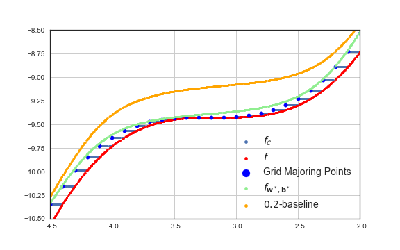
Figure 1: $1D$ synthetic experiment  with Grid Based Majoring Points

The function $f_{1}$, $f_{\mathcal{C}}$, $f_{\mathbf{w}^{*},\mathbf{b}^{*}}$ for Grid Based Majoring Points and the $0.2$-baseline  are displayed on Figure 1, on the interval $[-4.5,-2]$. The function $f_{1}f$, the Grid Based Majoring Points  and $f_{\mathbf{w}^{*},\mathbf{b}^{*}}$ for Grid Based Majoring Points and the $0.2$-baseline are displayed on Figure 2, on the interval $[0.8,1.2]$. The function $f_{1}$, the Data Adapted Majoring Points, the sample $(x_{i},f_{1}(x_{i}))_{i=1..n}$ and $f_{\mathbf{w}^{*},\mathbf{b}^{*}}$ for Data Adapted Majoring Points  are displayed on Figure 3, on the interval $[-5.5,0]$.

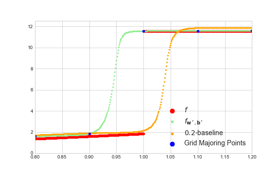
Figure 2: Discontinuity of $1D$ synthetic experiment  with Grid Based Majoring Points

Figure 3: $1D$ synthetic experiment  with Data Adapted Majoring Points

We clearly see that the adaptive Majoring Points aggregate in dyadic manner in the vicinity of the discontinuities. We also see on Figure 2 how Majoring Points permit to anticipate the discontinuity and construct an overestimation. The density of Majoring Points depends on the slope of $f_{1}$. This permits to reduce the approximation error. Also, $f_{\mathbf{w}^{*},\mathbf{b}^{*}}$ passes in the vicinity of the Majoring Points  and provides a good approximation that overestimates $f$.

The MAE, RMSE, OP and FG are provided in Table 1 for the $0$-baseline, the $0.5$-baseline, $f_{\mathcal{C}}$ and the ONN for three types of Majoring Points. We see that the RMSE worsen as we impose guarantees and approach the realistic scenario where the surrogate is easy to compute and does not require too much memory consumption.

	$n$	MAE	RMSE	OP	FG
$0$-baseline	200	N/A	-.04	51.9 %	NO
$0.5$-baseline	200	0.5	0.59	99.5%	NO
$f_{\mathcal{C}}$	200	N/A	0.10	100 %	YES
ONN with GMP	200	0.24	0.23	100%	YES
ONN with FMP	200	0.23	0.55	100%	YES
ONN with DMP	500	0.82	0.60	100%	YES

Table 1: Metrics - $1D$ synthetic experiment 

$2D$ synthetic experiment

The same phenomenon described on $1D$ synthetic experiment occur in dimension $2$. We only illustrate here the difference between the Grid Based Majoring Points, Function Adapted Majoring Points and Data Adapted Majoring Points  for the function

$$\forall(x,y)\in[0;15]^{2}\qquad g(x,y)=f_{1}\left(\sqrt{x^{2}+y^{2}}-10\right)$$

where $f_{1}$ is the function defined in (16).

We display, on Figure 5, the Function Adapted Majoring Points returned by the Dichotomy Algorithm. The density of points is correlated with the amplitude of the gradient of the function. Algorithm 1 permit to diminish the number of Majoring Points. For instance, for the $2D$ synthetic example for $\varepsilon=0.1$, the Grid Based Majoring Points counts $22500$ points. The Function Adapted Majoring Points counts $14898$ points, for $\varepsilon=0.5$, and $3315$, for $\varepsilon=2$. The Data Adapted Majoring Points counts $8734$ points, for $\varepsilon=0.5$, and $1864$, for $\varepsilon=2$.

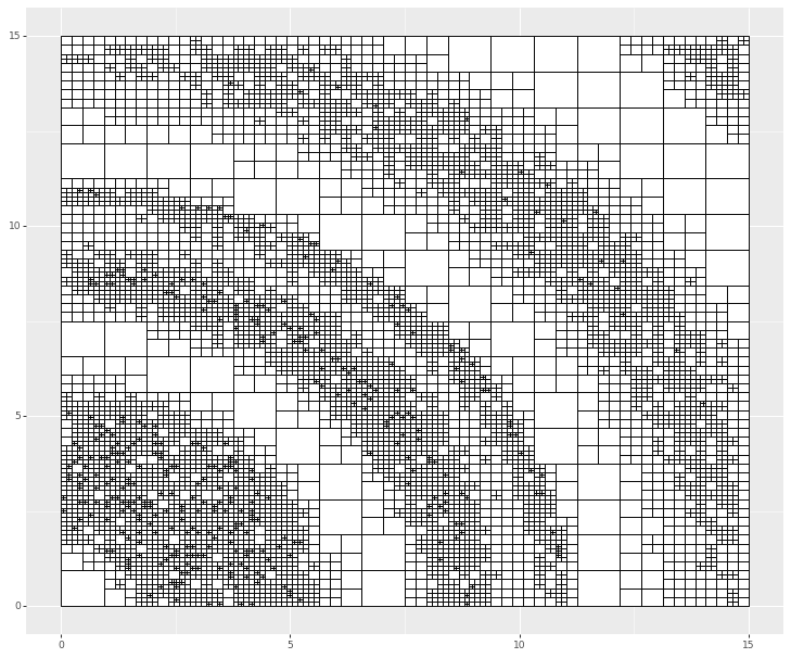
(a) Complete domain

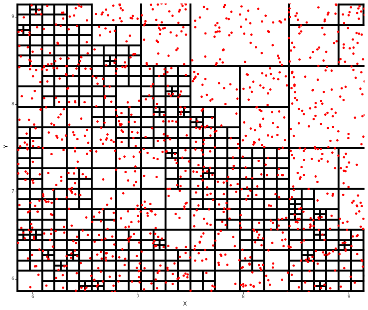
(b) Zoom on the discontinuity

Figure 4: Data Majoring Points grid

On Figure 4, we represent the dataset and the cover obtained using Algorithm 1 for the synthetic $2D$ example. The inputs $a_{i}$ of the corresponding Majoring Points are displayed on Figure 5.

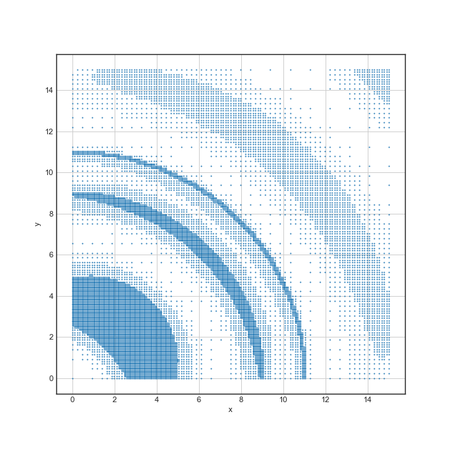
(a) Complete domain

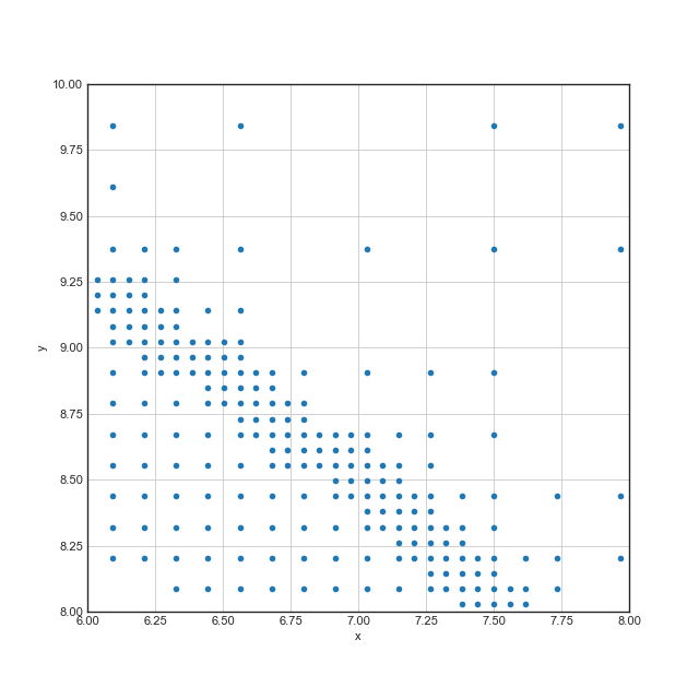
(b) Zoom on the discontinuity

Figure 5: Function Adapted Majoring Points on synthetic $2D$ $f$.

Industrial application

Method	$n$	$n_{maj}$	RMSE	MAE	OP	FG
$0$-baseline	150k	150k	3.3	N/A	65.1%	NO
$300$-baseline	150k	150k	302.6	300.0	100%	NO
ONN with GMP	150k	150k	309.3	262.7	100%	YES
ONN with DMP	150k0	110k	445.7	N/A	N/A	YES

Table 2: Results on the industrial dataset

The method developed in this paper provides formal guarantees of overestimation that are safety guarantee directly applicable in critical embedded systems.

The construction of surrogate functions is an important subject in industry (Lathuilière et al. 2019; Biannic et al. 2016; Jian et al. 2017; Sudakov et al. 2019). In this work, we are considering an industrial and heavy simulation code that has six inputs $d=6$ and one output and that represents a complex physic phenomenon of an aircraft. The output is an non-decreasing function. During the flight, given flight conditions $x$ the output $f(x)$ is compared to a threshold and the result of the test launch an action. When we replace $f$ by the overestimating surrogate $f_{\mathbf{w}^{*},\mathbf{b}^{*}}$, the airplane launches the action less often. However, the airplane only launches the action when the action is guaranteed to be safe.

The industrial dataset contains $n=150000$ examples on a static grid and another set of $150000$ sampled according to the uniform distribution on the whole domain. For each inputs, the reference computation code is used to generate the associated true output.

We compare $0$-baseline,$300$-baseline with the ONN learned on Grid Based Majoring Points and Data Adapted Majoring Points methods. All the methods are learned on the static grid except OON with Data Adapted Majoring Points. The table 2 presents the metrics for the different methods. The results are acceptable for the application and memory requirement to store and embed the neural network is $17088$ floating numbers. It is one order of magnitude smaller than the size of the dataset.

5 Conclusion - Future Work

We presented a method that enables to formally guarantee that a prediction of a monotonic neural network will always be in an area that preserves the safety of a system. This is achieved by the construction of the network, the utilization of majoring points and the learning phase, which allows us to free ourselves from a massive testing phase that is long and costly while providing fewer guarantees.

Our work have limitations on functions that can be a safely approximate, but this is a first step toward a safe use of neural networks in critical applications. Nevertheless, this can already be used in simple safety critical systems that verify our hypotheses. Future works will look on possibility to leverage the utilization of the monotonic hypothesis. Another direction of improvement is to build smarter algorithms that require less majoring points thanks to a better adaptation to the structure of the function. In particular, this should permit to apply the method to functions whose is input space is of larger dimension, when they have the proper structure.

References

- Amos, Xu, and Kolter (2017) Amos, B.; Xu, L.; and Kolter, J. Z. 2017. Input Convex Neural Networks. In Proceedings of the 34th International Conference on Machine Learning - Volume 70, ICML’17, 146–155. JMLR.org.
- Anthony and Bartlett (1999) Anthony, M.; and Bartlett, P. L. 1999. Neural Network Learning: Theoretical Foundations. Cambridge University Press. ISBN 0 521 57353 X. URL http://www.stat.berkeley.edu/~bartlett/nnl/index.html. 404pp. ISBN 978-0-521-57353-X. Reprinted 2001, 2002. Paperback edition 2009; ISBN 978-0-521-11862-0.
- Bartlett et al. (2019) Bartlett, P. L.; Harvey, N.; Liaw, C.; and Mehrabian, A. 2019. Nearly-tight VC-dimension and Pseudodimension Bounds for Piecewise Linear Neural Networks. Journal of Machine Learning Research 20(63): 1–17.
- Bianchi and Jakubowicz (2012) Bianchi, P.; and Jakubowicz, J. 2012. Convergence of a multi-agent projected stochastic gradient algorithm for non-convex optimization. IEEE transactions on automatic control 58(2): 391–405.
- Biannic et al. (2016) Biannic, J.; Hardier, G.; Roos, C.; Seren, C.; and Verdier, L. 2016. Surrogate models for aircraft flight control: some off-line and embedded applications. AerospaceLab Journal (12): pages–1.
- Boopathy et al. (2019) Boopathy, A.; Weng, T.-W.; Chen, P.-Y.; Liu, S.; and Daniel, L. 2019. Cnn-cert: An efficient framework for certifying robustness of convolutional neural networks. In Proceedings of the AAAI Conference on Artificial Intelligence, volume 33, 3240–3247.
- Daniels and Velikova (2010) Daniels, H.; and Velikova, M. 2010. Monotone and partially monotone neural networks. IEEE Transactions on Neural Networks 21(6): 906–917.
- Fischer et al. (2019) Fischer, M.; Balunovic, M.; Drachsler-Cohen, D.; Gehr, T.; Zhang, C.; and Vechev, M. 2019. DL2:- Training and Querying Neural Networks with Logic. In International Conference on Machine Learning.
- Gal and Ghahramani (2016) Gal, Y.; and Ghahramani, Z. 2016. Bayesian Convolutional Neural Networks with Bernoulli Approximate Variational Inference. In 4th International Conference on Learning Representations (ICLR) workshop track.
- Harvey, Liaw, and Mehrabian (2017) Harvey, N.; Liaw, C.; and Mehrabian, A. 2017. Nearly-tight VC-dimension bounds for piecewise linear neural networks. In Conference on Learning Theory, 1064–1068.
- Jakubovitz, Giryes, and Rodrigues (2019) Jakubovitz, D.; Giryes, R.; and Rodrigues, M. R. 2019. Generalization error in deep learning. In Compressed Sensing and Its Applications, 153–193. Springer.
- Jian et al. (2017) Jian, Z.-D.; Chang, H.-J.; Hsu, T.-s.; and Wang, D.-W. 2017. Learning from Simulated World-Surrogates Construction with Deep Neural Network. In SIMULTECH, 83–92.
- Julian, Kochenderfer, and Owen (2019) Julian, K. D.; Kochenderfer, M. J.; and Owen, M. P. 2019. Deep Neural Network Compression for Aircraft Collision Avoidance Systems. Journal of Guidance, Control, and Dynamics 42(3): 598–608. ISSN 1533-3884. doi:10.2514/1.g003724. URL http://dx.doi.org/10.2514/1.G003724.
- Katz et al. (2017) Katz, G.; Barrett, C.; Dill, D. L.; Julian, K.; and Kochenderfer, M. J. 2017. Reluplex: An efficient SMT solver for verifying deep neural networks. In International Conference on Computer Aided Verification, 97–117. Springer.
- Keren, Cummins, and Schuller (2018) Keren, G.; Cummins, N.; and Schuller, B. 2018. Calibrated prediction intervals for neural network regressors. IEEE Access 6: 54033–54041.
- Lang (2005) Lang, B. 2005. Monotonic Multi-layer Perceptron Networks as Universal Approximators. In Duch, W.; Kacprzyk, J.; Oja, E.; and Zadrożny, S., eds., Artificial Neural Networks: Formal Models and Their Applications – ICANN 2005, 31–37. Berlin, Heidelberg: Springer Berlin Heidelberg. ISBN 978-3-540-28756-8.
- Lathuilière et al. (2019) Lathuilière, S.; Mesejo, P.; Alameda-Pineda, X.; and Horaud, R. 2019. A comprehensive analysis of deep regression. IEEE transactions on pattern analysis and machine intelligence .
- Mirman, Gehr, and Vechev (2018) Mirman, M.; Gehr, T.; and Vechev, M. 2018. Differentiable Abstract Interpretation for Provably Robust Neural Networks. In Dy, J.; and Krause, A., eds., Proceedings of the 35th International Conference on Machine Learning, volume 80 of Proceedings of Machine Learning Research, 3578–3586. Stockholmsmässan, Stockholm Sweden: PMLR. URL http://proceedings.mlr.press/v80/mirman18b.html.
- Nguyen and Hein (2017) Nguyen, Q.; and Hein, M. 2017. The loss surface of deep and wide neural networks. In Proceedings of the 34th International Conference on Machine Learning-Volume 70, 2603–2612. JMLR. org.
- Pearce et al. (2018) Pearce, T.; Brintrup, A.; Zaki, M.; and Neely, A. 2018. High-Quality Prediction Intervals for Deep Learning: A Distribution-Free, Ensembled Approach. In Proceedings of the 35th International Conference on Machine Learning, ICML, 4072–4081.
- Raghunathan, Steinhardt, and Liang (2018) Raghunathan, A.; Steinhardt, J.; and Liang, P. 2018. Certified Defenses against Adversarial Examples.
- Sill (1998) Sill, J. 1998. Monotonic Networks. In Jordan, M. I.; Kearns, M. J.; and Solla, S. A., eds., Advances in Neural Information Processing Systems 10, 661–667. MIT Press. URL http://papers.nips.cc/paper/1358-monotonic-networks.pdf.
- Sudakov et al. (2019) Sudakov, O.; Koroteev, D.; Belozerov, B.; and Burnaev, E. 2019. Artificial Neural Network Surrogate Modeling of Oil Reservoir: a Case Study. In International Symposium on Neural Networks, 232–241. Springer.
- Tagasovska and Lopez-Paz (2019) Tagasovska, N.; and Lopez-Paz, D. 2019. Single-Model Uncertainties for Deep Learning. arXiv preprint arXiv:1811.00908, To appear in NeurIPS .
- Yao and Tong (1996) Yao, Q.; and Tong, H. 1996. Asymmetric least squares regression estimation: a nonparametric approach. Journal of nonparametric statistics 6(2-3): 273–292.