Unique equilibrium states for geodesic flows on flat surfaces with singularities

Abstract.

Consider a compact surface of genus $\geq 2$ equipped with a metric that is flat everywhere except at finitely many cone points with angles greater than $2\pi$. Following the technique in the work of Burns, Climenhaga, Fisher, and Thompson, we prove that sufficiently regular potential functions have unique equilibrium states if the singular set does not support the full pressure. Moreover, we show that the pressure gap holds for any potential which is locally constant on a neighborhood of the singular set. Finally, we establish that the corresponding equilibrium states have the $K$-property, and closed regular geodesics equidistribute.

1. Introduction

We examine the uniqueness of equilibrium states for geodesic flows on a specific class of CAT(0) surfaces, those where the negative curvature is concentrated at a finite set of points. Translation surfaces are examples of such surfaces. A translation surface $X$ is a pair $(X,\omega)$ where $X$ is a Riemann surface of genus $g$, and $\omega$ is a holomorphic one-form on $X$. The zeroes of this holomorphic one-form occur at a finite set of points. The one-form $\omega$ defines a metric which is flat everywhere except at its zeroes. At the zeroes the metric has a conical singularity with angle $2(n+1)\pi$, where $n$ is the order of the zero. For a more in-depth overview of translation surfaces see [Wri15, Zor06].

In [BCFT18], the authors prove that under certain conditions, a unique equilibrium state exists for potentials associated to the geodesic flow on a closed, rank-one manifold with nonpositive sectional curvature (an example of a CAT(0) space without singularities). The conditions are a Hölder continuous potential and a pressure gap, that is, topological pressure of the flow restricted to the singular set is strictly less than pressure of the flow overall. The singular set they consider is all the vectors in the unit tangent bundle with rank larger than one.

When the singular set is empty – for example in strictly negative curvature – every Hölder potential has a unique equilibrium state. When the singular set is non-empty, an additional condition is necessary as the geodesic flow is nonuniformly hyperbolic. Restricting the pressure of the flow on the singular set is a way of describing the flow of the singular set as having a small enough impact on the system as a whole that uniqueness is still guaranteed.

The natural way to define a geodesic flow on CAT(0) surfaces is to look at the flow on the set of all geodesics (see Section 2.1). Denote by $GS$ the set of all geodesics on the surface $S$ (see (2.1)).

In this paper, we study the uniqueness of equilibrium states for the geodesic flow described above (see Definition 2.5), as we are guaranteed existence for continuous potentials by entropy-expansivity of the flow (see Lemma 2.17). In particular, we use the technique of [BCFT18] in our setting and define the singular set to be the set of geodesics which never encounter any cone points or, when they do, turn by angle exactly $\pm\pi$.

Remark.

Some other settings where the uniqueness of equilibrium states was studied are described in more detail below in the outline of the argument.

We prove the following:

Theorem A.

Let $g_{t}$ be the geodesic flow on $S$, a compact, connected surface of genus $\geq 2$ equipped with a metric that is flat everywhere except at finitely many cone points which have angle greater than $2\pi$. Let $\mathrm{Sing}$ be the singular set as defined in Definition 2.4. Consider $\phi\colon GS\to\mathbb{R}$ a Hölder continuous potential. If the pressure of the singular set is strictly less than the full topological pressure, i.e., $P(\mathrm{Sing},\phi)<P(\phi)$ (see Definitions 2.5 and  2.6), then $\phi$ has a unique equilibrium state $\mu$ that has the $K$-property (see Definition 2.2).

It is natural to ask for which potentials we have the pressure gap (i.e., the condition $P(\mathrm{Sing},\phi)<P(\phi)$) in Theorem A. The following theorem establishes the pressure gap for a large class of Hölder continuous potentials, and thus uniqueness of equilibrium states.

Theorem B (Theorem 7.1 and Corollary 7.8).

Let $S$, $GS$, and $g_{t}$ be as in Theorem A. Let $\phi\colon GS\rightarrow\mathbb{R}$ be a Hölder continuous function which is locally constant on a neighborhood of $\mathrm{Sing}$, or which is sufficiently close to a constant in the uniform norm (see Corollary 7.8 for a precise statement of ‘sufficiently close’). Then $P(\mathrm{Sing},\phi)<P(\phi)$.

As a nice corollary (Corollary 7.7 below) we have $h_{top}(g_{t}|_{\mathrm{Sing}})<h_{top}(g_{t})$ for our flows.

We slightly improve the case $\phi=0$ from Ricks’s result [Ric21, Theorem B] by showing that the unique measure of maximal entropy for the geodesic flow on $S$ has the K-property which is stronger than mixing. Using the Patterson-Sullivan construction, Ricks builds a measure of maximal entropy $\mu$ [Ric17] and shows it is unique by asymptotic geometry arguments [Ric21]. We note that Ricks’s result holds for any compact, geodesically complete, locally CAT(0) space such that the universal cover admits a rank-one axis.

A natural question is whether the techniques in this paper can be extended to the more general CAT(0), rank-one setting in which Ricks works. The present paper can be viewed as a first step in that direction, but working in the general CAT(0) setting presents real difficulties right from the outset of the argument. In particular, without the Riemannian structure present in [BCFT18] or the flat surface structure we exploit, it is not clear to us what the right candidate for the singular set for would be, or how to find a function like $\lambda$ (see Section 3) to aid in producing an orbit decomposition.

We call a geodesic that is not in $\mathrm{Sing}$ regular. Using strong specification for a certain collection of ‘good’ orbit segments, we show that weighted regular closed geodesics equidistribute to these equilibrium states (see Section 8 for details).

Theorem C (Theorem 8.1).

Let $\phi$ be as in Theorem B and $\mu_{\phi}$ is the corresponding equilibrium state. Then, $\mu_{\phi}$ is the weak* limit of weighted regular closed geodesics.

1.1. Outline of the argument

A general scheme for proving that unique equilibrium states exist was developed by Climenhaga and Thompson in [CT16], building on ideas of Bowen in [Bow75] which were extended to flows in [Fra77]. To prove that there are unique equilibrium states for a flow $\{f_{t}\}$ and a potential $\phi$ on a compact metric space $X$, Climenhaga and Thompson ask for the following (see [CT16, Theorems A & C]):

• The pressure of obstructions to expansivity, $P^{\perp}_{exp}(\phi)$ (see Definition 2.7), is smaller than $P(\phi)$, and

• There are three collections of orbit segments $\mathcal{P},\mathcal{G},\mathcal{S}$, that we call collections of prefixes, good orbit segments, and suffixes, respectively, such that each orbit segment can be decomposed into a prefix, a good part, and a suffix (see [BCFT18, Definition 2.3]), satisfying

  • $\mathcal{G}$ has the weak specification property at any scale (Definition 2.8),

  • $\phi$ has the Bowen property on $\mathcal{G}$ (Definition 2.9), and

  • $P([\mathcal{P}]\cup[\mathcal{S}],\phi)<P(\phi)$.

This scheme was implemented for the geodesic flow on a closed rank-one manifold with nonpositive sectional curvature in [BCFT18] and, more generally, without focal points in [CKP20, CKP21]. Also, it was used to obtain the uniqueness of the measure of maximal entropy on certain manifolds without conjugate points in [CKW21] and on CAT(-1) spaces in [CLT20b].

Our proof follows a specific approach to satisfying the conditions in the above scheme which was applied in [BCFT18], and which allows us to reduce condition (III) to checking the pressure of an invariant subset of $GS$. Although the decomposition $(\mathcal{P,G,S})$ is in general very abstract, we choose the decomposition using a function $\lambda$ on the space of geodesics. This choice of decomposition also allows us to avoid having to deal with the sets $[\mathcal{P}]$ and $[S]$, which are discretized versions of $\mathcal{P}$ and $S$ necessary for technical counting arguments to be applied to some decompositions. We define the function $\lambda$, prove that it is lower semicontinuous, and describe how it gives rise to a decomposition in Section 3. For such a ‘$\lambda$-decomposition’, $\mathcal{P}=\mathcal{S}$ and, roughly speaking, orbit segments in $\mathcal{P}$ and $\mathcal{S}$ have small average values of $\lambda$ wheareas any initial or terminal segment of an element of $\mathcal{G}$ has average value of $\lambda$ which is not small. Furthermore, by utilizing a $\lambda$-decomposition, we are able to appeal to the following result:

Theorem 1.1 ([Cal22], Theorem 4.6).

Let $\mathcal{F}$ be a continuous flow on a compact metric space $X$, and let $\phi:X\to\mathbb{R}$ be continuous. Suppose the flow is asymptotically entropy-expansive, that $P^{\perp}_{\exp}(\phi)<P(\phi)$, and that $\lambda:X\to[0,\infty)$ is lower semicontinuous and bounded. If the $\lambda$-decomposition $(\mathcal{P},\mathcal{G},\mathcal{S})$ satisfies the following:

• $\mathcal{G}(\eta)$ has strong specification at all scales, for all $\eta>0$,

• $\phi$ has the Bowen property on $\mathcal{G}(\eta)$,

• $P(\bigcap_{t\in\mathbb{R}}(f_{t}\times f_{t})\tilde{\lambda}^{-1}(0),\Phi)<2P(\phi)$,

where $\Phi(x,y)=\phi(x)+\phi(y)$ and $\tilde{\lambda}(x,y)=\lambda(x)\lambda(y)$, then $(X,\mathcal{F},\phi)$ has a unique equilibrium state which has the $K$-property.

Theorem A will follow from Theorem 1.1 after we show that we can satisfy all conditions required. See Section 1.2 for the sections where each property is checked.

Our choice of $\lambda$ gives a connection between orbit segments in $\mathcal{P}$ and $\mathcal{S}$ and the singular set $\mathrm{Sing}$ (see Definition 2.4). The singular set is also the source of the obstructions to expansivity (see Lemma 2.16). These connections are useful for proving the two ‘pressure gap’ properties Theorem 1.1 calls for: $P^{\perp}_{exp}(\phi)<P(\phi)$ and $P(\bigcap_{t\in\mathbb{R}}(f_{t}\times f_{t})\tilde{\lambda}^{-1}(0),\Phi)<2P(\phi)$. In particular, in our case $\bigcap_{t\in\mathbb{R}}f_{t}\lambda^{-1}(0)=\mathrm{Sing}$.

Remark.

The strong specification property on $\mathcal{G}$ in Theorem 1.1 is used to obtain that the equilibrium state has the $K$-property. The weak specification property on $\mathcal{G}$ is enough to guarantee the existence of a unique equilibrium state.

Remark.

The K-property implies strong mixing of all orders.

1.2. Organization of the paper

The paper is organized as follows. In Section 2 we provide definitions of and background on the main objects and tools of this paper and we record some basic geometric results which will be used throughout the paper. The main steps for the proof of Theorem A according to Theorem 1.1 are in Sections 3 (the $\lambda$-decomposition), 4 and 5 (the specification property for $\mathcal{G}$), and 6 (the Bowen property for $\mathcal{G}$).

We obtain Theorem B in Section 7, first proving the pressure gap condition for potentials which are locally constant on a neighborhood of $\mathrm{Sing}$, and then using this result to note that the same gap holds for potentials with sufficiently small total variation. Theorem C (the equidistribution result) is proved in Section 8.

2. Background

2.1. Setting and Definitions

Throughout, $S$ denotes a compact, connected surface of genus $\geq 2$ equipped with a metric which is flat everywhere except at finitely many conical points which have angles larger than $2\pi$ (See Figure 1). We assume $S$ is oriented by passing to the oriented double cover if necessary. $Con$ denotes the set of conical points on $S$ and denote by $\mathcal{L}(p)$ the total angle at a point $p\in S$. In particular, $\mathcal{L}(p)=2\pi$ if $p\notin Con$ and $\mathcal{L}(p)>2\pi$ if $p\in Con$. Note that in the special case of a translation surface, $\mathcal{L}(p)$ is always an integer multiple of $2\pi$, but we make no such restriction here. Denote by $\tilde{S}$ the universal cover of $S$, and note that $\tilde{S}$ is a complete $\mathrm{CAT}(0)$ space (see, e.g. [BH99] for definitions and basic results on $\mathrm{CAT}(0)$ spaces). Throughout, tildes denote the obvious lifts to the universal cover.

Since $\tilde{S}$ is $\mathrm{CAT}(0)$, any $\tilde{p},\tilde{q}$ are connected by a unique geodesic segment. Throughout, we will denote this segment by $[\tilde{p},\tilde{q}].$

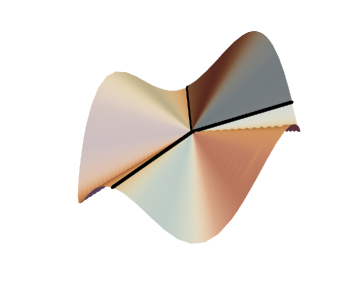
Figure 1. A large-angle cone point, embedded in $\mathbb{R}^{3}$. Away from the cone point, the surface is flat under the intrinsic metric – it is the union of lines in $\mathbb{R}^{3}$ and so has Gaussian curvature zero. The dark lines show a geodesic segment hitting the cone point and its two continuations with turning angles $\pm\pi$; these geodesics are in $\mathrm{Sing}$. All continuations of the geodesic with line segments passing through the dark shaded region are geodesics. The spread of the geodesic continuations in this region is exactly the source of ‘hyperbolicity’ for the geodesic flow in these spaces.

Let $GS$ be the set of all (parametrized) geodesics in $S$. That is,

$$GS=\{\gamma\colon\mathbb{R}\rightarrow S\mid\gamma\text{ is a local isometry}\}.$$ (2.1)

We endow $GS$ with the following metric:

$$d_{GS}(\gamma_{1},\gamma_{2})=\inf\limits_{\tilde{\gamma}_{1},\tilde{\gamma}_{2}}\int_{-\infty}^{\infty}d_{\tilde{S}}(\tilde{\gamma}_{1}(t),\tilde{\gamma}_{2}(t))e^{-2|t|}\,dt,$$ (2.2)

where the infimum is taken over all lifts $\tilde{\gamma}_{i}$ of $\gamma_{i}$ to $G\tilde{S}$ for $i=1,2$. $GS$ serves as an analogue of the unit tangent bundle in our setting. (Indeed, for a Riemannian surface, $GS$ is homeomorphic to $T^{1}S$.) It is necessary to examine this more complicated space as geodesics in $S$ are not determined by a tangent vector – they may branch apart from each other at points in $Con$. In this setting, the metric $d_{GS}$ records the idea that two geodesics in $GS$ are close if their images in $S$ are nearby for all $t$ in some large interval $[-T,T]$.

Geodesic flow on $GS$ comes from shifting the parametrization of a geodesic:

$$(g_{t}\gamma)(s)=\gamma(s+t).$$

The normalizing factor 2 in our definition of $d_{GS}$ ensures that $g_{t}$ is a unit-speed flow with respect to $d_{GS}$. (Showing this is a completely straight-forward computation, using the fact that $d_{\tilde{S}}(\tilde{\gamma}(t),\tilde{\gamma}(s+t))=s$).

We recall two definitions of the $K$-property of an invariant measure. See Section 10.8 in [CFS82] for a proof of the equivalence of these definitions (known as completely positive entropy and $K$-mixing, respectively) with the original definition of the $K$-property, as well as more details about other equivalent definitions.

Definition 2.1.

A flow-invariant measure $\mu$ has the $K$-property if $(X,(g_{t}),\mu)$ has no non-trivial zero entropy factors (i.e., the Pinsker factor is trivial).

This definition can be reformulated as a statement about mixing in the following manner.

Definition 2.2.

A flow-invariant measure $\mu$ has the $K$-property if for all $t\neq 0$, for all $k\geq 1$, and all measurable sets $A_{0},A_{1},\ldots,A_{k}$ we have

$$\lim\limits_{n\rightarrow\infty}\sup\limits_{B\in\mathcal{C}_{n}(A_{1},\ldots,A_{k})}\left|\mu(A_{0}\cap B)-\mu(A_{0})\mu(B)\right|=0,$$

where $\mathcal{C}_{n}(A_{1},\ldots,A_{k})$ is the minimal $\sigma$-algebra generated by $g_{tr}(A_{j})$ for $1\leq j\leq k$ and natural $r\geq n$.

Remark.

The K-property implies strong mixing of all orders. We recall that an invariant measure $\mu$ is strongly mixing of all orders if for all $k\geq 1$ and all measurable sets $A_{0},A_{1},\ldots,A_{k}$ we have

$$\lim\limits_{t_{1}\rightarrow\infty,\,t_{j+1}-t_{j}\rightarrow\infty}\mu(A_{0}\cap g_{t_{1}}(A_{1})\cap\ldots\cap g_{t_{k}}(A_{k}))=\prod_{j=0}^{k}\mu(A_{j}).$$

A key tool in our analysis of the geodesic flow on $S$ will be the turning angle of a geodesic at a cone point. We note that although $S$ is not smooth at $p\in Con$, there is a well-defined space of directions at $p$, $S_{p}S$, and a well-defined notion of angle (see, e.g. [BH99, Ch. II.3]). In the angular metric, $S_{p}S$ is a circle of total circumference $\mathcal{L}(p)$.

Definition 2.3.

Let $\gamma\in GS$. The turning angle of $\gamma$ at time $t$ is $\theta(\gamma,t)\in(-\frac{1}{2}\mathcal{L}(\gamma(t)),\frac{1}{2}\mathcal{L}(\gamma(t))]$ and is the signed angle between the segments $[\gamma(t-\delta),\gamma(t)]$ and $[\gamma(t),\gamma(t+\delta)]$ (for sufficiently small $\delta>0$). A positive (resp. negative) sign for $\theta$ corresponds to a counterclockwise (resp. clockwise) rotation with respect to the orientation of $[\gamma(t-\delta),\gamma(t)]$.

Since $\gamma$ is a geodesic, $|\theta(\gamma,t)|-\pi\geq 0$ for any $t\in\mathbb{R}$. If $\gamma(t)\not\in Con$, then $\theta(\gamma,t)=\pi$.

Definition 2.4.

We define the singular geodesics in $S$ as

$$\mathrm{Sing}=\{\gamma\in GS:|\theta(\tilde{\gamma},t)|=\pi\quad\forall t\in\mathbb{R}\}.$$

Since $\mathrm{Sing}$ is defined in terms of properties of full geodesics, it is $g_{t}$-invariant. Geodesics not in $\mathrm{Sing}$ turn by some angle $\neq\pi$ at a cone point. This is an open condition, so $\mathrm{Sing}$ is closed and hence compact.

The geodesics in $\mathrm{Sing}$ either never encounter any cone points or, when they do, turn by angle exactly $\pm\pi$. They serve as an analogue of the singular set in the Riemannian setting of [BCFT18], i.e., geodesics which remain entirely in zero-curvature regions of the surface. In both cases the idea is that a singular geodesic never takes advantage of the geometric features of the surface (either its negative curvature regions or its large-angle cone points) to produce hyperbolic dynamical behavior. We note here a potentially confusing aspect of this terminology: a singular geodesic in this paper avoids the ‘singular,’ i.e. non-smooth, points of $Con$, or treats them as if they are not ‘singular.’

We introduce some classical notions of thermodynamical formalism.

Definition 2.5.

Consider a function $\phi\colon GS\rightarrow\mathbb{R}$ that we refer as a potential function. The pressure for $\phi$ is

$$P(\phi)=\sup\limits_{\mu}\left(h_{\mu}(g_{t})+\int_{GS}\phi d\mu\right),$$

where $\mu$ varies over all invariant Borel probability measures for $g_{t}$ and $h_{\mu}(g_{t})$ is the measure-theoretic entropy with respect to the geodesic flow.

An invariant Borel probability measure $\mu_{\phi}$ (if it exists) such that

$$P(\phi)=h_{\mu_{\phi}}(g_{t})+\int_{GS}\phi d\mu_{\phi}$$

is an equilibrium state for $\phi$.

Definition 2.6.

$P(\mathrm{Sing},\phi)$ is the pressure of the potential $\phi|_{\mathrm{Sing}}$ on the compact and flow-invariant set $\mathrm{Sing}$ (see Definition 2.4).

Below, we discuss some of the necessary definitions to apply the Climenhaga-Thompson machinery.

Definition 2.7.

Let $\varepsilon>0$. The non-expansive set at scale $\varepsilon$ for the flow $g_{t}$ is

$$\operatorname{NE}(\varepsilon)=\{\gamma\in GS\mid\Gamma_{\varepsilon}(\gamma)\not\subset g_{[-s,s]}\gamma\text{ for all }s>0\},$$

where

$$\Gamma_{\varepsilon}(\gamma)=\{\xi\in GS\mid d_{GS}(g_{t}\gamma,g_{t}\xi)\leq\varepsilon\quad\forall t\in\mathbb{R}\}.$$

The pressure of obstructions to expansivity for a potential $\phi$ is

$$P^{\perp}_{\exp}(\phi)=\lim\limits_{\varepsilon\downarrow 0}\sup\left\{h_{\mu}(g_{1})+\int_{GS}\phi\,d\mu\bigm{|}\mu(\operatorname{NE}(\varepsilon))=1\right\},$$

where the supremum is taken over all $g_{t}$-invariant ergodic probability measures $\mu$ on $GS$ such that $\mu(\operatorname{NE}(\varepsilon))=1$.

In other words, a geodesic is in the complement of $\operatorname{NE}(\varepsilon)$ if the only geodesics which stay $\varepsilon$ close to it for all time are contained in its own orbit. A flow is expansive if $\operatorname{NE}(\varepsilon)$ is empty for all sufficiently small $\varepsilon$. The presence of flat strips in our setting means our flow will not be expansive, but for small $\varepsilon$, the complement of $\operatorname{NE}(\varepsilon)$ will turn out to be a sufficiently rich set to use in our arguments.

In the interest of concision, we omit the formal definition of an orbit decomposition, referring instead to [CT16]. We will use a specific type of decomposition which has been studied in [CT22, Cal22], and we will primarily use results from those two papers. We note however that results from [CT16] hold for our decompositions as well, as it is written for a more general class of decomposition. We discuss this more in Section 8, where we will need to appeal to a few results directly from [CT16]. Identify a pair $(\gamma,t)\in GS\times[0,\infty)$ with the orbit segment $\{g_{s}\gamma\mid s\in[0,t]\}$. An orbit decomposition is a method of decomposing any orbit segment into three subsegments, a prefix, a central good segment, and a suffix. We denote the collections of these segments by $\mathcal{P},\mathcal{G}$, and $\mathcal{S}$ respectively. The $\lambda$-decompositions that we use in this paper are orbit decompositions which decompose orbit segments based on a lower semicontinuous function $\lambda$. Our choices for the function $\lambda$ and the associated parameter $\eta>0$ will be discussed in detail in Section 3, but the idea is this. The function $\lambda$ measures the amount of ‘hyperbolic’ behavior seen by the geodesic; in accord with our intuition that cone points are the source of this behavior, $\lambda$ will be based on turning angles at these points. A segment is ‘good’ for our purposes (i.e., in $\mathcal{G}(\eta)$) if it experiences a lot of hyperbolicity; otherwise, it is in $\mathcal{P}=\mathcal{S}$:

• $\mathcal{G}=\mathcal{G}(\eta)$ consists of all $(\gamma,t)$ such that the average value of $\lambda$ over every initial and terminal segment of $(\gamma,t)$ is at least $\eta$, and

• $\mathcal{P}=\mathcal{S}=\mathcal{B}(\eta)$ consists of all $(\gamma,t)$ over which the average value of $\lambda$ is less than $\eta.$

We can define both specification and the Bowen property for an arbitrary collection of orbit segments $\mathcal{G}\subset GS\times[0,\infty)$. In both cases, by taking $\mathcal{G}=GS\times[0,\infty)$, one retrieves the definitions for the full dynamical system.

Definition 2.8.

We say that $\mathcal{G}$ has weak specification if for all $\varepsilon>0$, there exists $\tau>0$ such that for any finite collection $\{(x_{i},t_{i})\}_{i=1}^{n}\subset\mathcal{G}$, there exists $y\in GS$ that $\varepsilon$-shadows the collection with transition times $\{\tau_{i}\}_{i=1}^{n}$ at most $\tau$ between orbit segments. In other words, for $1\leq i\leq n$, there exists $\tau_{i}\in[0,\tau]$ and $y\in GS$ such that

$$d_{GS}(g_{t+s_{i}}y,g_{t}x_{i})\leq\varepsilon\text{ for }0\leq t\leq t_{i}$$

where $s_{k}=\sum_{j=1}^{k-1}t_{j}+\tau_{j}$. We will refer to such $\tau$ as a specification constant.

We say that $\mathcal{G}$ has strong specification when we can always take each $\tau_{j}=\tau$ in the above definition.

Definition 2.9.

Given a potential $\phi:GS\to\mathbb{R}$, we say that $\phi$ has the Bowen property on $\mathcal{G}$ if there is some $\varepsilon>0$ for which there exists a constant $K>0$ such that

$$\sup\left\{\left|\int_{0}^{t}\phi(g_{r}x)-\phi(g_{r}y)\,dr\right|\bigm{|}(x,t)\in\mathcal{G}\text{ and }d_{GS}(g_{r}y,g_{r}x)\leq\varepsilon\text{ for }0\leq r\leq t\right\}\leq K.$$

Remark.

If $\phi$ has the Bowen property on a collection of orbit segments $\mathcal{G}$ at some scale $\varepsilon>0$, it in turn has the Bowen property on $\mathcal{G}$ at all smaller scales $\varepsilon^{\prime}<\varepsilon$.

There is also a definition of topological pressure for collections of orbit segments. However, by using Theorem 1.1, we sidestep this complication.

Finally, we adapt a piece of terminology from flat surfaces to our somewhat more general setting.

Definition 2.10.

A geodesic segment with both endpoints in $Con$ and no cone points in its interior is called a saddle connection. A saddle connection path is composed of saddle connections joined so that the turning angle at each cone point is at least $\pi$. Note that with this definition all saddle connection paths are geodesic segments.

2.2. Basic geometric results

In this section we collect a few basic results on the geometry of $S$, $\tilde{S}$, $GS$, and $G\tilde{S}$ which will be used in our subsequent arguments.

The following two lemmas relate the metric $d_{GS}$ to the metric $d_{S}$ on the surface itself, and will be useful for a number of our calculations below. First, we note that if two geodesics are close in $GS$, then they are close in $S$ at time zero.

Lemma 2.11 ([CLT20b], Lemma 2.8).

For all $\gamma_{1},\gamma_{2}\in GS$,

$$d_{S}(\gamma_{1}(0),\gamma_{2}(0))\leq 2d_{GS}(\gamma_{1},\gamma_{2}).$$

Furthermore, for $s,t\in\mathbb{R}$, $d_{S}(\gamma_{1}(s),\gamma_{2}(t))\leq 2d_{GS}(g_{s}\gamma_{1},g_{t}\gamma_{2}).$

Conversely, if two geodesics are close in $S$ for a significant interval of time surrounding zero, then they are close in $GS$:

Lemma 2.12 ([CLT20b], Lemma 2.11).

Let $\varepsilon$ be given and $a<b$ arbitrary. There exists $T=T(\varepsilon)>0$ such that if $d_{S}(\gamma_{1}(t),\gamma_{2}(t))<\varepsilon/2$ for all $t\in[a-T,b+T]$, then $d_{GS}(g_{t}\gamma_{1},g_{t}\gamma_{2})<\varepsilon$ for all $t\in[a,b]$. For small $\varepsilon$, we can take $T(\varepsilon)=-\log(\varepsilon)$.

A similar, and more specialized result which we will need later in the paper (see the proof of Proposition 6.2) is the following

Lemma 2.13.

Suppose that $d_{S}(\gamma_{1}(t),\gamma_{2}(t))=0$ for all $t\in[a,b]$. Then, for all $t\in[a,b]$, $d_{GS}(g_{t}\gamma_{1},g_{t}\gamma_{2})\leq e^{-2\min\{|t-a|,|t-b|\}}$.

Proof.

For any $x\geq 0$, $\int_{x}^{\infty}(s-x)e^{-2s}ds=\frac{1}{4}e^{-2x}$. In the setting of the Lemma, since the distance between the geodesics is zero on $[a,b]$ and since geodesics move at unit speed,

$$d_{GS}(g_{t}\gamma_{1},g_{t}\gamma_{2})\leq\int_{-\infty}^{a}2(a-s)e^{-2|t-s|}ds+\int_{b}^{\infty}2(s-b)e^{-2|t-s|}ds.$$

Quick changes of variables show that this is equal to $\int_{|t-a|}^{\infty}2(s-|t-a|)e^{-2s}ds+\int_{|t-b|}^{\infty}2(s-|t-b|)e^{-2s}ds=\frac{1}{2}(e^{-2|t-a|}+e^{-2|t-b|})$, and the Lemma follows. ∎

The geodesic flow has the following Lipschitz property:

Lemma 2.14 ([CLT20a], Lemma 2.5).

Fix a $T>0$. Then, for any $t\in[0,T]$, and any pair of geodesics $\gamma,\xi\in GS$,

$$d_{GS}(g_{t}\gamma,g_{t}\xi)<e^{2T}d_{GS}(\gamma,\xi).$$

We need the following four geometric facts.

Lemma 2.15.

• There exists some $d_{0}>0$ such that $\tilde{S}$ contains no flat $d_{0}\times d_{0}$ square.

• There exists some $\eta_{0}>0$ such that the excess angle at every cone point in $S$ is at least $\eta_{0}$.

• There exists some $\ell_{0}>0$ such that the length of every saddle connection is at least $\ell_{0}$.

• There exists some $\theta_{0}>0$ such that the excess angle at every cone point in $S$ is at most $\theta_{0}$.

Proof.

These follow immediately from the compactness of $S$ and the fact that $S$ having genus at least two implies $Con\neq\emptyset.$ ∎

We note here that $\mathrm{Sing}$ is the source of the non-expansivity for our geodesic flow:

Lemma 2.16.

For all $\varepsilon>0$ less than half the injectivity radius of $S$, $\operatorname{NE}(\varepsilon)\subset\mathrm{Sing}$.

Proof.

Suppose $\gamma\in\operatorname{NE}(\varepsilon)$ and that $\varepsilon$ is smaller than half the injectivity radius of $S$. Then, there exists $\xi\in GS$ which is not in the orbit of $\gamma$ such that $d_{GS}(g_{t}\gamma,g_{t}\xi)\leq\varepsilon$ for all $t\in\mathbb{R}$. By Lemma 2.11, $d_{S}(\gamma(t),\xi(t))\leq 2\varepsilon$ for all $t\in\mathbb{R}$. In particular, using our assumption on $\varepsilon$, there exist lifts $\tilde{\gamma}$ and $\tilde{\xi}$ such that $d_{\tilde{S}}(\tilde{\gamma}(t),\tilde{\xi}(t))\leq 2\varepsilon$ for all $t\in\mathbb{R}$. By the Flat Strip Theorem ([Bal95, Corollary 5.8 (ii)]), there is an isometric embedding $\mathbb{R}\times[a,b]\to\tilde{S}$ sending $\mathbb{R}\times\{a\}$ to the image of $\tilde{\gamma}$ and $\mathbb{R}\times\{b\}$ to the image of $\tilde{\xi}$.

Since $\tilde{\xi}$ is not in the orbit of $\tilde{\gamma}$, we must have $a\neq b$ and the isometrically embedded strip is non-degenerate. But this immediately implies that for all $t$, $|\theta(\tilde{\gamma},t)|=\pi$ as $\tilde{\gamma}$ always turns at angle $\pi$ on the side to which the embedded flat strip lies. Therefore, $\gamma\in\mathrm{Sing}$. ∎

Recall that a flow is called entropy-expansive if for sufficiently small $\varepsilon$, $\sup\{h_{top}(g_{t}|_{\Gamma_{\varepsilon}(\gamma)})\mid\gamma\in GS\}=0$.

Lemma 2.17 ([Ric21], Lemma 20).

The geodesic flow in our setting is entropy-expansive.

Proof.

This is proven by Ricks in [Ric21] for geodesic flow on a CAT(0) space. This covers our setting, but Ricks uses a slightly different definition of the metric on $GS$ than we do, so we outline the argument here.

Fix $\varepsilon$ less than half the injectivity radius of $S$. Lift $\gamma$ to $\tilde{\gamma}\in G\tilde{S}$. Any geodesics $\xi\in\Gamma_{\varepsilon}(\gamma)$ lift to $\tilde{\xi}\in\Gamma_{\varepsilon}(\tilde{\gamma})$. They are either of the form $g_{t}\tilde{\gamma}$ for $|t|<\varepsilon$, or are parallel to $\tilde{\gamma}$ in a flat strip containing $\tilde{\gamma}$. The flow on $\Gamma_{\varepsilon}(\tilde{\gamma})$ is thus isometric, and so $h_{top}(g_{t}|_{\Gamma_{\varepsilon}(\gamma)})=0$. ∎

Lemma 2.18.

Given any closed geodesic $\gamma\subset S$, there is a closed saddle connection path which is homotopic to $\gamma$ and has the same length as $\gamma$.

Proof.

Assume $\gamma$ contains a point $p\in Con$. Then the desired closed saddle connection path is the geodesic that starts at $p$ and traces $\gamma$.

Suppose $\gamma\subset S\setminus Con$, and so $\tilde{\gamma}\subset\tilde{S}\setminus\widetilde{Con}$. Fix an orientation of $\tilde{\gamma}$ and consider the variation $\tilde{\gamma}_{r}$ of curves given by sliding $\tilde{\gamma}$ to its left (so the variational field is perpendicular to $\tilde{\gamma}$ and to its left with respect to $\tilde{\gamma}$’s orientation). Since $\tilde{\gamma}\subset\tilde{S}\setminus\widetilde{Con}$ and $\gamma$ is closed, there is a nonzero lower bound on the distance from $\tilde{\gamma}$ to $\widetilde{Con}$. Therefore, for all sufficiently small $r$, $\tilde{\gamma}_{r}$ is defined. The projections to $S$, $\gamma_{r}$ and $\gamma$, form the boundary of a flat cylinder in $S$. Thus, $\gamma_{r}$ is a geodesic with length equal to that of $\gamma$.

Let $r^{*}$ be the supremum of all $r>0$ for which $\tilde{\gamma}_{\rho}$ is defined for all $\rho\in[0,r]$. Note that if no supremum exists, $\tilde{\gamma}$ bounds a flat half-space in $\tilde{S}$, which contains a fundamental domain for $S$ since $S$ is compact. This would imply $S$ is flat (with no cone points), a contradiction. Therefore letting $r\to r^{*}$ from below, $\tilde{\gamma}_{r}$ limits uniformly on a path, and therefore necessarily a geodesic, containing at least one point in $\widetilde{Con}$ with the same length as $\tilde{\gamma}$. The image of this curve in $S$ (with appropriate parametrization) is the saddle connection path we want. ∎

In the proof of Lemma 2.20 and in some later proofs we will use the following construction.

Definition 2.19.

Let $\tilde{\gamma}$ be a geodesic segment in $\tilde{S}$ with endpoint $p$. The cone around $\tilde{\gamma}$ with vertex $p$ and angle $\psi$ is the set of all points $q$ in $\tilde{S}$ such that the unique geodesic segment joining $p$ and $q$ makes angle $\leq\psi$ with $\tilde{\gamma}$ at $p$. (In Section 3, Figure 2 shows such cones in the context of the proof of Lemma 3.8.)

Lemma 2.20.

For any $\zeta\in Con$ there exists a closed geodesic $\alpha$ passing through $\zeta$ with turning angle greater than $\pi$ at $\zeta$.

Proof.

Let $\zeta$ be a cone point with $\mathcal{L}(\zeta)=2\pi+\beta$ for $\beta>0$. Lift $\zeta$ to $\tilde{\zeta}$ in $\tilde{S}$ and let $\tilde{c}$ be a geodesic with $\tilde{c}(0)=\tilde{\zeta}$ and turning angle $\theta(\tilde{c},0)=\pi+\frac{\beta}{2}$. Let $C_{1}$ be the cone around $\tilde{c}(-\infty,0)$ with vertex $\tilde{\zeta}=\tilde{c}(0)$ and angle $\frac{\beta}{8}$; let $C_{2}$ be the cone around $\tilde{c}(0,\infty)$ with vertex $\tilde{\zeta}=\tilde{c}(0)$ and angle $\frac{\beta}{8}$. By construction, any geodesic connecting a point in $C_{1}\setminus\{\tilde{\zeta}\}$ to a point in $C_{2}\setminus\{\tilde{\zeta}\}$ must pass through $\tilde{\zeta}$ with turning angle $\geq\pi+\frac{\beta}{4}$.

Let $\mathcal{F}$ be a fundamental domain contained in $C_{1}$. Let $g\in\pi_{1}(S)$ be such that $g\mathcal{F}\subset C_{2}$. ($\mathcal{F}$ and $g$ exist as both $C_{1}$ and $C_{2}$ contain arbitrarily large balls and $S$ is compact.) Let $\alpha$ be the closed geodesic representative of $g$ in $S$. (It will become clear in a moment why $\alpha$ is unique up to parametrization.) Lift $\alpha$ to $\tilde{\alpha}$ with $\tilde{\alpha}(0)\in\mathcal{F}$. Then $\tilde{\alpha}(\ell(\alpha))\in g\mathcal{F}$. As noted above, this forces $\tilde{\alpha}$ to pass through $\tilde{\zeta}$ and turn with angle $>\pi$. Therefore, $\alpha$ is the desired geodesic (and it is unique up to parametrization since it cannot belong to a flat cylinder). ∎

3. The $\lambda$-decomposition

We now turn to the main arguments of the paper. First, following the ideas in [BCFT18], we establish the decomposition $(\mathcal{P,G,S})$ as a ‘$\lambda$-decomposition’ using the function $\lambda$ in Definition 3.3 which is defined through two auxiliary functions that view the stable and unstable parts of any given geodesic. Throughout this section, fix $s>0$ such that $2s$ is less than the shortest saddle connection of $S$. Below we omit in the notation the dependence of functions on $s$.

Definition 3.1.

We define $\lambda^{uu}\colon GS\rightarrow[0,\infty)$ by

$$\lambda^{uu}(\gamma)=\frac{|\theta(\gamma,c)|-\pi}{\max\{s,c\}},$$

where $c\geq 0$ is the first time that $\gamma(c)$ hits a cone point and turns with angle strictly greater than $\pi$ (naturally, we set $\lambda^{uu}(\gamma)=0$ in case $c=\infty$).

Definition 3.2.

We define $\lambda^{ss}\colon GS\rightarrow[0,\infty)$ by

$$\lambda^{ss}(\gamma)=\frac{|\theta(\gamma,c)|-\pi}{\max\{s,|c|\}},$$

where $c\leq 0$ is the most recent time that $\gamma(c)$ has hit a cone point and turned with angle strictly greater than $\pi$ (naturally, we set $\lambda^{ss}(\gamma)=0$ in case $c=-\infty$).

We now define our function $\lambda$ so that near cone points at which geodesics turn with angle greater than $\pi$, it measures the turning angle at that cone point (multiplied by a constant), and far from a cone point, it measures both distance and turning angle from both the previous and next cone point.

Definition 3.3.

Let $\lambda^{uu}$ and $\lambda^{ss}$ be functions defined in Definitions 3.1 and  3.2, respectively. We define $\lambda\colon GS\rightarrow[0,\infty)$ by

$$\lambda(\gamma)=\begin{cases}\lambda^{ss}(\gamma)&\text{if there exists }c\in(-s,0]\text{ such that }|\theta(\gamma,c)|-\pi>0,\\ \lambda^{uu}(\gamma)&\text{if there exists }c\in[0,s)\text{ such that }|\theta(\gamma,c)|-\pi>0,\\ \min\{\lambda^{ss}(\gamma),\lambda^{uu}(\gamma)\}&\text{otherwise}.\end{cases}$$

Observe that it is well-defined when $\gamma(0)$ is a cone point, as in that case, $\lambda^{uu}(\gamma)=\lambda^{ss}(\gamma)$.

We prove several properties of $\lambda$.

Proposition 3.4.

If $\lambda(\gamma)=0$, then $\lambda(g_{t}\gamma)=0$ either for all $t\geq 0$ or for all $t\leq 0$.

Proof.

If $\lambda(\gamma)=0$, then $\gamma$ does not turn at a cone point in the interval $(-s,s)$, and so, $\lambda^{uu}(\gamma)=0$ or $\lambda^{ss}(\gamma)=0$. In the first case, this implies that $\gamma$ never turns at a cone point in the future. Therefore, for all $t\geq 0$, $\lambda(g_{t}\gamma)=\lambda^{uu}(g_{t}\gamma)=0$. A similar argument holds with $t\leq 0$ if $\lambda^{ss}(\gamma)=0$. ∎

As corollaries, we have:

Corollary 3.5.

$\bigcap_{t\in\mathbb{R}}g_{t}\lambda^{-1}(0)=\mathrm{Sing}$.

Corollary 3.6.

If $\lambda(\gamma)=0$, then $d(g_{t}\gamma,\mathrm{Sing})\to 0$ either as $t\to\infty$ or as $t\to-\infty$.

Proof.

Without loss of generality, assume $\lambda(g_{t}\gamma)=0$ for all $t\geq 0$. Then, $\gamma$ does not turn at a cone point in $[0,\infty)$, and we can define $r:=\max\{t:|\theta(\gamma,t)|>\pi\}$ to be the most recent cone point in the past at which $\gamma$ turns. Define a singular geodesic $\gamma_{\mathrm{Sing}}$ as $\gamma_{\mathrm{Sing}}(t)=\gamma(t)$ for all $t>r$, and for all cone points $t\leq r$, $\gamma_{\mathrm{Sing}}$ turns with angle $\pi$. Then, $g_{t}\gamma$ and $g_{t}\gamma_{\mathrm{Sing}}$ agree on increasingly long intervals, and by Lemma 2.13 for $t>r$,

$$d_{GS}(g_{t}\gamma,\mathrm{Sing})\leq d_{GS}(g_{t}\gamma,g_{t}\gamma_{\mathrm{Sing}})\leq e^{-2(t-r)}.$$

The proof if $\lambda(g_{t}\gamma)=0$ holds similarly, but sending $t\to-\infty$ instead. ∎

Furthermore, this allows us to show that the pressure gap for the product flow (condition (3) of Theorem 1.1) is implied by the pressure gap $P(\mathrm{Sing},\phi)<P(\phi)$ that we will establish in Section 7.

Proposition 3.7.

(Following [CT22, Proposition 5.1]) Setting $\Phi(x,y)=\phi(x)+\phi(y)$ and $\tilde{\lambda}(x,y)=\lambda(x)\lambda(y)$ we have $P(\bigcap_{t\in\mathbb{R}}(g_{t}\times g_{t})(\tilde{\lambda})^{-1}(0),\Phi)\leq P(\phi)+P(\mathrm{Sing},\phi)$. In particular, if $P(\mathrm{Sing},\phi)<P(\phi)$, then $P(\bigcap_{t\in\mathbb{R}}(g_{t}\times g_{t})(\tilde{\lambda})^{-1}(0),\Phi)<2P(\phi)$.

Proof.

The Variational Principle [Wal82, Theorem 9.10] tells us that

$$P\left(\bigcap_{t\in\mathbb{R}}(g_{t}\times g_{t})(\tilde{\lambda}^{-1}),\Phi\right)=\sup\left\{P_{\nu}(\Phi)\bigm{|}\nu\text{ is flow invariant and }\nu\left(\bigcap_{t\in\mathbb{R}}(g_{t}\times g_{t})(\tilde{\lambda}^{-1})\right)=1\right\},$$

where $P_{\nu}(\Phi):=h_{\nu}(g_{1}\times g_{1})+\int\Phi\,d\nu$ denotes the measure-theoretic pressure of $(\bigcap_{t\in\mathbb{R}}(g_{t}\times g_{t})(\tilde{\lambda}^{-1}),(g_{t}\times g_{t}),\Phi,\nu).$ More generally, this relationship holds for any continuous flow, continuous potential, and compact, flow-invariant subset.

Consequently, we let $\nu$ be an invariant measure supported on $\bigcap_{t\in\mathbb{R}}(g_{t}\times g_{t})(\tilde{\lambda})^{-1}(0)$, and let

$$A=\bigcap_{t\in\mathbb{R}}(g_{t}\times g_{t})(\tilde{\lambda})^{-1}(0)\cap(\mathrm{Reg}\times\mathrm{Reg}).$$

We will show that $\nu(A)=0$ by showing that it contains no recurrent points. Assume for contradiction that $(\gamma_{1},\gamma_{2})\in A$ is a recurrent point, and then assume without loss of generality that $\lambda(\gamma_{1})=0$. Since $\gamma_{1}\notin\mathrm{Sing}$, it follows that $d_{GS}(\gamma_{1},\mathrm{Sing})=c>0$, which from recurrence, implies that there exists a sequence $t_{k}\to\infty$ such that $d_{GS}(g_{t_{k}}\gamma_{1},\mathrm{Sing})>\frac{c}{2}$, with a similar claim holding in backwards time. However, we also know that $d_{GS}(g_{t}\gamma_{1},\mathrm{Sing})\to 0$ as $t\to\infty$, or as $t\to-\infty$ by Corollary 3.6. Thus, we have arrived at a contradiction. Hence, $\nu$ is supported on the complement of $\mathrm{Reg}\times\mathrm{Reg}$, which is $(\mathrm{Sing}\times GS)\cup(GS\times\mathrm{Sing})$.

Thus,

$$P\left(\bigcap_{t\in\mathbb{R}}(g_{t}\times g_{t})(\tilde{\lambda}^{-1}(0)),\Phi\right)\leq P\left((\mathrm{Sing}\times GS)\cup(GS\times\mathrm{Sing}),\Phi\right)\leq P(\mathrm{Sing},\phi)+P(GS,\phi).$$

The first inequality is by the Variational Principle. The second inequality is due to the fact that the pressure of the union of two compact invariant sets is the maximum of the pressure of each individual set [Pes97, Theorem 11.2(3)], and in this case, the pressure of each component of the union is at most $P(\mathrm{Sing},\phi)+P(GS,\phi)$ by [Wal82, Theorem 9.8(v)]. ∎

We have also constructed $\lambda$ so that it is lower semicontinuous.

Lemma 3.8.

Let $s>0$ be such that $2s$ is less than the shortest saddle connection of $S$. Then, $\lambda$ defined in Definition 3.3 is lower semicontinuous.

Proof.

Let $\gamma\in GS$. We show that for any $\varepsilon>0$ there exists $\delta>0$ such that $\lambda(\gamma)-\varepsilon<\lambda(\xi)$ for all $\xi\in GS$ such that $d_{GS}(\gamma,\xi)<\delta$. To ease the arguments below slightly, we work in $\tilde{S}$ with lifts $\tilde{\gamma},\tilde{\xi}$ so that $d_{G\tilde{S}}(\tilde{\gamma},\tilde{\xi})=d_{GS}(\gamma,\xi)$. Recall that by Lemma 2.11, if $d_{G\tilde{S}}(\tilde{\gamma},\tilde{\xi})<\delta$ then $d_{\tilde{S}}(\tilde{\gamma}(0),\tilde{\xi}(0))<2\delta$.

If $\lambda(\gamma)=0$, then we are done as $\lambda$ is a non-negative function. Therefore, for the rest of the argument we assume that $\lambda(\gamma)>0$.

Case 1: Suppose there exists $c\in(-s,s)$ such that $\psi:=|\theta(\tilde{\gamma},c)|-\pi>0$. Denote $\tilde{\gamma}(c)=p$. We show that there exists $\delta>0$ such that $p\in\tilde{\xi}((-s,s))$.

Let $C_{1}$ be the cone around $\tilde{\gamma}((c,s))$ with vertex $p$ and angle $\psi^{\prime}=\min\{\frac{\psi}{2},\frac{\pi}{4}\}$. Let $C_{2}$ be the cone around $\tilde{\gamma}((-s,c))$ with vertex $p$ and angle $\psi^{\prime}$. (See Figure 2.) Set

$$\delta=\frac{1}{2}\min\left\{\frac{1}{8}e^{-2s}(s-|c|)\sin\psi^{\prime},\quad\frac{1}{2}(s-d_{S}(\tilde{\gamma}(0),p)),\quad\min\{1,\varepsilon s/8\}(2+e^{2|c|})^{-1}\int_{0}^{s-|c|}2te^{-2t}dt\right\}.$$ (3.1)

Then, we choose $u_{1}=\frac{c+s}{2},u_{2}=\frac{c-s}{2}$ and $\delta_{1}=\frac{s-c}{4}\sin\psi^{\prime},\delta_{2}=\frac{c+s}{4}\sin\psi^{\prime}>0$ so that $B_{1}:=B(\tilde{\gamma}(u_{1}),\delta_{1})\subset C_{1}\cap B(\tilde{\gamma}(0),s)$ and $B_{2}:=B(\tilde{\gamma}(u_{2}),\delta_{2})\subset C_{2}\cap B(\tilde{\gamma}(0),s)$. By Lemmas 2.11 and 2.14, since $\delta<\frac{1}{8}e^{-2s}(s-|c|)\sin\psi^{\prime}$, if $d_{G\tilde{S}}(\tilde{\gamma},\tilde{\xi})<\delta$ then $\tilde{\xi}$ passes through $B_{1}$ and $B_{2}$. Since any two points in a CAT(0)-space are connected by a unique geodesic segment and by our construction of $C_{1}$ and $C_{2}$, we obtain that if $d_{G\tilde{S}}(\tilde{\gamma},\tilde{\xi})<\delta$ then $\tilde{\xi}$ passes through $p$. Furthermore, since $2\delta+d_{S}(\tilde{\gamma}(0),p)<s$, by Lemma 2.11 and the triangle inequality for the triangle with vertices $\tilde{\xi}(0),\tilde{\gamma}(0)$, and $p$, we have $p\in\tilde{\xi}((-s,s))$ if $d_{G\tilde{S}}(\tilde{\gamma},\tilde{\xi})<\delta$. Let $t_{0}\in(-s,s)$ be such that $\tilde{\xi}(t_{0})=p$. Moreover, $|t_{0}-c|\leq 2\delta$.

Figure 2. The argument for Case 1 in Lemma 3.8. The geodesic segments connecting points in $B_{2}$ and $B_{1}$ meet at the cone point $p$ with angle $\geq\pi$ on both sides. Any geodesic connecting points in $B_{2}$ and $B_{1}$ must run through $p$.

By the triangle inequality,

$$d_{\tilde{S}}(\tilde{\xi}(t_{0}+t),\tilde{\gamma}(c+t))\leq d_{\tilde{S}}(\tilde{\xi}(t_{0}+t),\tilde{\xi}(c+t))+d_{\tilde{S}}(\tilde{\xi}(c+t),\tilde{\gamma}(c+t))=|t_{0}-c|+d_{\tilde{S}}(\tilde{\xi}(c+t),\tilde{\gamma}(c+t)).$$

Let $\tilde{\xi}_{1}=g_{t_{0}}\tilde{\xi}$ and $\tilde{\gamma}_{1}=g_{c}\tilde{\gamma}$. Then, by the above inequality and Lemma 2.14,

$$d_{G\tilde{S}}(\tilde{\xi}_{1},\tilde{\gamma}_{1})\leq 2\delta+e^{2|c|}\delta=(2+e^{2|c|})\delta.$$ (3.2)

Moreover, for all $t\in(0,s-c]$, we obtain that

$$d_{\tilde{S}}(\tilde{\xi}_{1}(t),\tilde{\gamma}_{1}(t))=\left\{\begin{aligned} &2t\qquad&\text{if}\qquad&\alpha\geq\pi,\\ &2t\sin(\alpha/2)\qquad&\text{if}\qquad&0\leq\alpha\leq\pi,\end{aligned}\right.$$

where $\alpha$ is the (unsigned) angle between the outward trajectories of $\tilde{\gamma}_{1}$ and $\tilde{\xi}_{1}$ from the cone point $p$.

If $\alpha\geq\pi$, then $d_{G\tilde{S}}(\tilde{\xi}_{1},\tilde{\gamma}_{1})\geq\int_{0}^{s-c}2te^{-2t}dt$, which is not possible by (3.2) and the choice of $\delta$ (see (3.1)).

Consider $\alpha\in[0,\pi)$. Then we have that

$$\sin(\alpha/2)<\delta(2+e^{2|c|})\left(\int_{0}^{s-c}2te^{-2t}dt\right)^{-1}.$$ (3.3)

Let $\beta$ be the (unsigned) angle between the inward trajectories $\tilde{\gamma}_{1}$ and $\tilde{\xi}_{1}$ at $p$. Similarly to the argument above, we obtain that for $\delta$ as defined in (3.1),

$$\sin(\beta/2)<\delta(2+e^{2|c|})\left(-\int_{-s-c}^{0}2te^{2t}dt\right)^{-1}.$$ (3.4)

Using (3.3) and (3.4),

$$|\lambda(\gamma)-\lambda(\xi)|=\frac{1}{s}\left||\theta(\tilde{\gamma},c)|-|\theta(\tilde{\xi},t_{0})|\right|\leq\frac{1}{s}(\alpha+\beta)\leq C\delta,$$

where $C=\frac{8}{s}(2+e^{2|c|})\left(\int_{0}^{s-|c|}2te^{-2t}dt\right)^{-1}$. Thus, for our choice of $\delta$ (see (3.1)), we have $|\lambda(\gamma)-\lambda(\xi)|<\varepsilon$.

Case 2: Assume there exists $c_{1}\leq-s$ and $c_{2}\geq s$ such that $\psi_{1}:=|\theta(\tilde{\gamma},c_{1})|-\pi>0$ and $\psi_{2}:=|\theta(\tilde{\gamma},c_{2})|-\pi>0$. Denote $\tilde{\gamma}(c_{1})=p_{1}$ and $\tilde{\gamma}(c_{2})=p_{2}$.

Let $C_{1}$ be the cone around the segment $\tilde{\gamma}((c_{1},-s])$ if $c_{1}\neq-s$ or $\tilde{\gamma}((-2s,-s))$ otherwise with vertex $p_{1}$ and angle $\psi^{\prime}=\frac{\min\{\psi_{1},\psi_{2},\pi\}}{4}$. Let $C_{2}$ be the cone around the segment $\tilde{\gamma}([s,c_{2}])$ if $c_{2}\neq s$ or $\tilde{\gamma}((s,2s))$ otherwise, with vertex $p_{2}$ and angle $\psi^{\prime}$. Set

$$c=\min\{|c_{1}|,c_{2}\}\ \text{ and }\ \delta=\frac{1}{2}\min\left\{\frac{1}{8}e^{-2s}(c-s)\sin\psi^{\prime},\quad\min\{1,\varepsilon c/8\}(2e^{2c}+1)^{-1}\int_{c}^{\infty}2te^{-2t}dt\right\}.$$ (3.5)

Similar to Case 1, by Lemmas 2.11 and 2.14 and the choice of $\delta$ in (3.5), if $d_{G\tilde{S}}(\tilde{\gamma},\tilde{\xi})<\delta$ then $\tilde{\xi}$ passes through $p_{1}$ and $p_{2}$. In particular, $\tilde{\gamma}$ and $\tilde{\xi}$ share a geodesic connecting $p_{1}$ and $p_{2}$. Therefore, there exists $d$ such that $g_{d}\tilde{\xi}(t)=\tilde{\gamma}(t)$ for $t\in[c_{1},c_{2}]$. Let $t_{1}$ and $t_{2}$ be such that $\tilde{\xi}(t_{1})=p_{1}$ and $\tilde{\xi}(t_{2})=p_{2}$. Then, $|t_{1}-c_{1}|\leq 2e^{2|c_{1}|}\delta$ and $|t_{2}-c_{2}|\leq 2e^{2c_{2}}\delta$ so $|d|\leq 2e^{2c}\delta$. Moreover, by the triangle inequality,

$$d_{G\tilde{S}}(g_{d}\tilde{\xi},\tilde{\gamma})\leq(2e^{2c}+1)\delta.$$ (3.6)

Let $\alpha_{1}$ and $\alpha_{2}$ be the (unsigned) angles between the inward and outward trajectories of $g_{d}\tilde{\xi}$ and $\tilde{\gamma}$ at $p_{1}$ and $p_{2}$, respectively. Similarly to Case 1, for our choice of $\delta$, we have $0\leq\alpha_{1},\alpha_{2}\leq\pi$,

$$\sin(\alpha_{1}/2)\leq\delta(2e^{2c}+1)\left(-\int_{c_{2}}^{\infty}2te^{2t}dt\right)^{-1},$$

and

$$\sin(\alpha_{2}/2)\leq\delta(2e^{2c}+1)\left(\int_{c_{1}}^{\infty}2te^{-2t}dt\right)^{-1}.$$

Therefore,

$$|\lambda^{ss}(\gamma)-\lambda^{ss}(\xi)|\leq C\delta\quad\text{and}\quad|\lambda^{uu}(\gamma)-\lambda^{uu}(\xi)|\leq C\delta,$$

where $C=\frac{8}{c}(2e^{2c}+1)\left(\int_{c}^{\infty}2te^{-2t}dt\right)^{-1}$.

Thus, if $t_{1}=c_{1}+d\leq-s$ and $t_{2}=c_{2}+d\geq s$, then $\lambda(\xi)=\min\{\lambda^{ss}(\xi),\lambda^{uu}(\xi)\}$ and we have $|\lambda(\gamma)-\lambda(\xi)|\leq C\delta<\varepsilon$.

Otherwise, $\lambda(\xi)\geq\min\{\lambda^{ss}(\xi),\lambda^{uu}(\xi)\}$ and we have $\lambda(\xi)\geq\lambda(\gamma)-C\delta>\lambda(\gamma)-\varepsilon$. ∎

Remark.

Note that for this construction of $\lambda$, we do not in general have upper semicontinuity. To see this, consider a geodesic $\gamma$ which turns with angle greater than $\pi$ at times $-s$ and $c$ for some $c>0$. Then, for all $r\in(0,s]$, $\lambda(g_{-r}\gamma)=\lambda^{ss}(g_{-r}\gamma)$, while $\lambda(\gamma)=\min\{\lambda^{ss}(\gamma),\lambda^{uu}(\gamma)\}$. Therefore, if $\lambda^{uu}(\gamma)<\lambda^{ss}(\gamma)$, we have that

$$\lambda(\gamma)=\lambda^{uu}(\gamma)<\lambda^{ss}(\gamma)=\lim_{r\downarrow 0}\lambda^{ss}(g_{-r}\gamma)=\lim_{r\downarrow 0}\lambda(g_{-r}\gamma).$$

This contradicts upper semicontinuity of $\lambda$.

Following §3 of [BCFT18], or Definition 3.4 in [CT22] (and formalizing the idea presented in Section 2.1), we define

$$\mathcal{G}(\eta)=\left\{(\gamma,t)\bigm{|}\int_{0}^{\rho}\lambda(g_{u}(\gamma))du\geq\eta\rho\quad\text{and}\quad\int_{0}^{\rho}\lambda(g_{-u}g_{t}(\gamma))du\geq\eta\rho\quad\text{for}\quad\rho\in[0,t]\right\}$$

and

$$\mathcal{B}(\eta)=\left\{(\gamma,t)\bigm{|}\int_{0}^{\rho}\lambda(g_{u}(\gamma))du<\eta\rho\right\}.$$

The decomposition we will take is $(\mathcal{P,G,S})=(\mathcal{B}(\eta),\mathcal{G}(\eta),\mathcal{B}(\eta))$ for a sufficiently small value of $\eta$ which will be determined below. We reiterate that because of our choice of decomposition, we do not need to consider the sets of orbit segments denoted by $[\mathcal{P}],[S]$, because of [CT22, Lemma 3.5].

While near cone points, positivity of $\lambda$ only gives us information about the closest cone point, and far from cone points, it gives us information about cone points on both sides. The following propositions help us quantify these relationships. Let $\theta_{0}$ be as in Lemma 2.15(d).

Proposition 3.9.

If $\lambda(\gamma)>\eta$, then there is a cone point in $\gamma[-\frac{\theta_{0}}{2\eta},\frac{\theta_{0}}{2\eta}]$ with turning angle at least $s\eta$ away from $\pm\pi$. In particular, if $(\gamma,t)\in\mathcal{G}(\eta)$, then there exist $t_{1},t_{2}\in[-\frac{\theta_{0}}{2\eta},\frac{\theta_{0}}{2\eta}]$ such that $\gamma(t_{1}),\gamma(t+t_{2})\in\operatorname{Con}$, with the turning angles at these cone points at least $s\eta$ away from $\pm\pi$.

Proof.

Since $\lambda(\gamma)>\eta$, either $\lambda^{uu}(\gamma)>\eta$ or $\lambda^{ss}(\gamma)>\eta$. If $\lambda^{uu}(\gamma)>\eta$, then by Definition 3.3 there is a $c\geq 0$ such that $\gamma(c)\in Con$ and $\lambda^{uu}(\gamma)=\frac{|\theta(\gamma,c)|-\pi}{\max\{s,c\}}$. The turning angle at $\gamma(c)$ satisfies $|\theta(\gamma,c)|-\pi\leq\theta_{0}/2$. Thus,

$$\eta<\lambda^{uu}(\gamma)\leq\frac{|\theta(\gamma,c)|-\pi}{c}\leq\frac{\theta_{0}/2}{c}$$

and $0\leq c\leq\frac{\theta_{0}}{2\eta}$. Furthermore,

$$\eta<\lambda^{uu}(\gamma)\leq\frac{|\theta(\gamma,c)|-\pi}{s}$$

so the turning angle of $\gamma$ at $c$ differs from $\pi$ by at least $s\eta.$

A similar argument applies if $\lambda^{ss}(\gamma)>\eta$. ∎

Finally, we collect a statement we will need in Section 7.

Lemma 3.10.

Given any $\eta>0$, there exists a $\delta>0$ such that $\lambda(\gamma)<\eta$ for all $\gamma\in B(\mathrm{Sing},2\delta)$.

Proof.

Let $\eta>0$ be given and suppose without generality it is small enough that $\frac{s\eta}{32}<1$. We argue in $\tilde{S}$. Suppose $\tilde{\gamma}\in B(\mathrm{Sing},2\delta)$ and, in particular, that $\tilde{\xi}\in\mathrm{Sing}$ with $d_{GS}(\tilde{\gamma},\tilde{\xi})<2\delta.$ We choose $\delta<\frac{s\theta_{0}}{64e^{4\theta_{0}/\eta}}$ and towards a contradiction suppose that $\lambda(\tilde{\gamma})>\frac{\eta}{2}.$ (Recall that $s$ is specified in Lemma 3.8, and $\eta_{0}$ is specified in Lemma 2.15(d).)

Since $\lambda(\tilde{\gamma})>\frac{\eta}{2}$, by Proposition 3.9, there exists a cone point in $\tilde{\gamma}[-\frac{\theta_{0}}{\eta},\frac{\theta_{0}}{\eta}]$ at which $\tilde{\gamma}$ turns with angle at least $\frac{s\eta}{2}$ away from $\pm\pi$. Say $\tilde{\gamma}$ hits that cone point at time $t_{0}\in[-\frac{\theta_{0}}{\eta},\frac{\theta_{0}}{\eta}].$

As $d_{G\tilde{S}}(\tilde{\gamma},\tilde{\xi})<2\delta$, by Lemma 2.14,

$$d_{G\tilde{S}}\left(g_{-\frac{2\theta_{0}}{\eta}}\tilde{\gamma},g_{-\frac{2\theta_{0}}{\eta}}\tilde{\xi}\right)<2\delta e^{\frac{4\theta_{0}}{\eta}}\ \ \mbox{ and }\ \ d_{G\tilde{S}}\left(g_{\frac{2\theta_{0}}{\eta}}\tilde{\gamma},g_{\frac{2\theta_{0}}{\eta}}\tilde{\xi}\right)<2\delta e^{\frac{4\theta_{0}}{\eta}}.$$

Then, by Lemma 2.11,

$$d_{\tilde{S}}\left(\tilde{\gamma}\left(-\frac{2\theta_{0}}{\eta}\right),\tilde{\xi}\left(-\frac{2\theta_{0}}{\eta}\right)\right)<4\delta e^{\frac{4\theta_{0}}{\eta}}\ \ \mbox{ and }\ \ d_{\tilde{S}}\left(\tilde{\gamma}\left(\frac{2\theta_{0}}{\eta}\right),\tilde{\xi}\left(\frac{2\theta_{0}}{\eta}\right)\right)<4\delta e^{\frac{4\theta_{0}}{\eta}}.$$

Consider the geodesic segment $c$ connecting $\tilde{\xi}(-\frac{2\theta_{0}}{\eta})$ and $\tilde{\gamma}(t_{0})$. The segment $c$ and $\tilde{\gamma}[-\frac{2\theta_{0}}{\eta},t_{0}]$ agree at $t_{0}$ and at time $-\frac{2\theta_{0}}{\eta}$, at least $\frac{\theta_{0}}{\eta}$ away with respect to $d_{\tilde{S}}$, are at most $4\delta e^{\frac{4\theta_{0}}{\eta}}$ apart. Comparing to a Euclidean triangle and using the CAT(0) property, the angle between these segments at $\tilde{\gamma}(t_{0})$ is at most $2\sin^{-1}[(4\delta e^{\frac{4\theta_{0}}{\eta}})/(2\frac{\theta_{0}}{\eta})]$. By our choice of $\delta$, this is less than $2\sin^{-1}[\frac{s\eta}{32}]<\frac{s\eta}{8}$. The same argument applies to the angle between $\tilde{\gamma}[t_{0},\frac{2\theta_{0}}{\eta}]$ and the segment $c^{\prime}$ from $\tilde{\gamma}(t_{0})$ to $\tilde{\xi}(\frac{2\theta_{0}}{\eta})$.

At $t_{0}$, $\tilde{\gamma}$ turns with angle at least $\frac{s\eta}{2}$ away from $\pm\pi$. Therefore, the concatenation of $c$ with $c^{\prime}$ turns with angle at least $\pi+\frac{s\eta}{4}$ on both sides, and hence is geodesic. By uniqueness of geodesic segments in $\tilde{S}$, $\xi[-\frac{2\theta_{0}}{\eta},\frac{2\theta_{0}}{\eta}]$ must agree with this concatenation. But this contradicts the fact that $\xi\in\mathrm{Sing}$. Therefore, $\lambda(\gamma)\leq\frac{\eta}{2}<\eta$ as desired. ∎

4. $\mathcal{G}(\eta)$ has weak specification (at all scales)

The goal of this section is to obtain Corollary 4.6 which shows that $\mathcal{G}(\eta)$ has weak specification at all scales.

Lemma 4.1.

(Compare with Lemma 3.8 in [Dan11]) Let $x\in S$ and $\beta$ be a geodesic ray with $\beta(0)=x$. Then, for any $\varepsilon>0$ there exist $T_{0}(\varepsilon)$ and a geodesic $c$ which connects $x$ with a point $z\in Con$ so that the length of $c$ is at most $T_{0}(\varepsilon)$ and $\angle_{x}(\beta,c)<\varepsilon$ where $\angle_{x}(a,b)$ is the angle at $x$ between geodesic segments $a$ and $b$.

Proof.

Let $\tilde{x}\in\tilde{S}$ be a lift of $x$ and $\tilde{\beta}$ a lift of $\beta$ with $\tilde{\beta}(0)=\tilde{x}$. Denote by $C_{\frac{\varepsilon}{2}}(\tilde{x},\tilde{\beta})$ the cone around $\beta$ with vertex $\tilde{x}$ and angle $\frac{\varepsilon}{2}$. Choose $T_{0}=T_{0}(\varepsilon)$ so large that an angle-$\varepsilon$ sector of a radius-$T_{0}$ Euclidean ball contains a ball of radius much larger than the diameter of $S$. Then $I=B_{T_{0}}(\tilde{x})\cap C_{\frac{\varepsilon}{2}}(\tilde{x},\tilde{\beta})$ is at least as large as this Euclidean sector and so must contain a fundamental domain of $S$. Then $\widetilde{Con}\cap Int(I)\neq\emptyset$, so let $\tilde{z}\in\widetilde{Con}\cap Int(I)$ such that $\tilde{z}$ is closest to $\tilde{x}$. The segment $\tilde{c}=\tilde{x}\tilde{z}$ is a geodesic of length at most $T_{0}$. The projection of $\tilde{c}$ to $S$ is the desired geodesic. ∎

Lemma 4.2.

For any $\delta>0$, there exists $T_{1}=T_{1}(\delta)$ such that for any $t>0$ and $(\gamma,t)\in\mathcal{G}(\eta)$, $(\gamma,t)$ is $\delta$-shadowed by a saddle connection path $\gamma_{e}$ in the following sense:

• $\ell(\gamma_{e})\leq t+2T_{1}$

• there exists $s_{0}\in[0,T_{1}]$ with the property that if $\gamma^{c}_{e}$ is any extension of $\gamma_{e}$ to a complete geodesic then $d_{GS}(g_{u}(\gamma),g_{u}(g_{s_{0}}(\gamma^{c}_{e})))\leq\delta$ for all $u\in[0,t]$.

In particular, if $t>\frac{\theta_{0}}{\eta}$, there exists a closed interval $I\supset[\frac{\theta_{0}}{2\eta},t-\frac{\theta_{0}}{2\eta}]$ such that $\gamma_{e}(s_{0}+u)=\gamma(u)$ for $u\in I$.

Proof.

As usual, we prove the result in $\tilde{S}$. Let $T=\max\{-\log(\delta),\frac{\theta_{0}}{2\eta},\frac{\ell_{0}}{4}\}$ where $\theta_{0}$ and $\ell_{0}$ are from Lemma 2.15. By Lemma 2.12, if we construct $\tilde{\gamma}_{e}$ such that $d_{\tilde{S}}(\tilde{\gamma}(u),\tilde{\gamma}_{e}(s_{0}+u))<\frac{\delta}{2}$ for all $u\in[-T,t+T]$, then $d_{GS}(g_{u}(\gamma),g_{u}(g_{s_{0}}(\gamma^{c}_{e})))\leq\delta$ for all $u\in[0,t]$. (See Figure 3 for the constructions in this proof.)

Figure 3. The construction of $\gamma_{e}$ in Lemma 4.2 around the left endpoint of $\gamma$. The sequence of $\alpha$-cones featured in the proof is shaded.

By Proposition 3.9, there exist $t_{0},t_{1}\in[-\frac{\theta_{0}}{2\eta},\frac{\theta_{0}}{2\eta}]$ such that $\tilde{\gamma}(t_{0}),\tilde{\gamma}(t+t_{1})\in\widetilde{Con}$, $|\theta(\tilde{\gamma},t_{0})|-\pi\geq s\eta$ and $|\theta(\tilde{\gamma},t+t_{1})|-\pi\geq s\eta$. Thus, there exist $s_{1}\in[-T,\frac{\theta_{0}}{2\eta}]$ and $s_{2}\in[-\frac{\theta_{0}}{2\eta},T]$ such that $\tilde{\gamma}(s_{1}),\tilde{\gamma}(t+s_{2})\in\widetilde{Con}$ and $\left(\tilde{\gamma}([-T,s_{1}))\cup\tilde{\gamma}((t+s_{2},t+T])\right)\cap\widetilde{Con}=\emptyset$.

If $s_{1}=-T$, then define $\tilde{\gamma}_{e}(u-s_{1})=\tilde{\gamma}(u)$ for $u\in[s_{1},t+s_{2}]$. Assume $s_{1}>-T$. Let $\eta_{0}$ be as in Lemma 2.15(b). Choose $\alpha<\frac{\ell_{0}}{4(T+\frac{\theta_{0}}{2\eta})}\min\{\eta_{0},\frac{\delta}{2(\frac{\theta_{0}}{2\eta}+T)}\}$. Let $\mathcal{C}$ be the cone in $\tilde{S}$ around $\tilde{\gamma}([-T,s_{1}])$ with angle $\alpha/2$. Note that $\alpha<\eta_{0}$, so any geodesic segment from a point in $\mathcal{C}$ to $\tilde{\gamma}(s_{1})$ can be concatenated with $\tilde{\gamma}([s_{1},t])$ to form a geodesic. By Lemma 4.1, there exists $T_{0}=T_{0}(\frac{\alpha}{2})\geq T+\frac{\theta_{0}}{2\eta}$ and a point $\tilde{p}_{1}$ in $\widetilde{Con}\cap\mathcal{C}$ such that $d_{\tilde{S}}(\tilde{p}_{1},\tilde{\gamma}(s_{1}))\leq T_{0}$. Choose $\tilde{p}_{1}$ as in the previous sentence minimizing the distance to $\tilde{\gamma}([-T_{0},s_{1}])$. If $d_{\tilde{S}}(\tilde{p}_{1},\tilde{\gamma}(s_{1}))\geq T+\frac{\theta_{0}}{2\eta}$, then let the initial segment of $\tilde{\gamma}_{e}$ be the geodesic segment $[\tilde{p}_{1},\tilde{\gamma}(s_{1})]$.

Otherwise, we repeat the argument above, applying Lemma 4.1 to construct an angle-$\alpha/2$ cone centered around the geodesic segment making angle $\pi+\frac{\alpha}{2}$ with $[\tilde{p}_{1},\tilde{\gamma}(s_{1})]$. We get a point $\tilde{p}_{2}\in\widetilde{Con}$ in this cone with $d_{\tilde{S}}(\tilde{p}_{1},\tilde{p}_{2})\leq T_{0}$, again chosen to minimize the distance to $\tilde{\gamma}([-T_{0},s_{1}])$. If $d_{\tilde{S}}(\tilde{p}_{2},\tilde{\gamma}(s_{1}))\geq T+\frac{\theta_{0}}{2\eta}$, then let the initial segment of $\tilde{\gamma}_{e}$ be the concatenation of geodesic segments $[\tilde{p}_{2},\tilde{p}_{1}]$ and $[\tilde{p}_{1},\tilde{\gamma}(s_{1})]$. This concatenation is a geodesic by the choice of $\alpha$ and the construction of the cone. Otherwise, repeat the procedure at $\tilde{p}_{2}$ and so on.

We will need to repeat this procedure at most $\frac{T+\frac{\theta_{0}}{2\eta}}{\ell_{0}}$ times. We extend the beginning of $\tilde{\gamma}_{e}$ constructed here with $[\tilde{\gamma}(s_{1}),\tilde{\gamma}(t+s_{2})]$ and then extend beyond $\tilde{\gamma}(t+s_{2})$ (if needed) similarly to the procedure at $\tilde{\gamma}(s_{1})$. Since the turning angles at each cone point are at least $\pi$, we obtain a saddle connection path $\tilde{\gamma}_{e}$.

Let $T_{1}=T+\frac{\theta_{0}}{2\eta}+T_{0}$. Let $s_{0}$ be such that $\tilde{\gamma}_{e}(s_{0}+s_{1})=\tilde{\gamma}(s_{1})$. Then $s_{0}\in[0,T_{1}]$. For $u\in[s_{1},s_{2}]$, $d_{\tilde{S}}(\tilde{\gamma}(u),\tilde{\gamma}_{e}(s_{0}+u))=0<\frac{\delta}{2}$, as desired. For $u\in[-T,s_{1}]$, note that the sequence of cones used in the proof have angles $\frac{\alpha}{2}$ and $\alpha<\frac{\ell_{0}}{4(T+\frac{\theta_{0}}{2\eta})}\frac{\delta}{2(\frac{\theta_{0}}{2\eta}+T)}$. There are at most $\frac{T+\frac{\theta_{0}}{2\eta}}{\ell_{0}}$ of these cones, each segment from $\tilde{p}_{i}$ to $\tilde{p}_{i+1}$ is at most length $T+\frac{\theta_{0}}{2\eta}$, and we always choose our cone points $\tilde{p}_{i}$ as close to $\tilde{\gamma}$ as we can. Therefore, the distance $d_{\tilde{S}}(\tilde{\gamma}(u),\tilde{\gamma}_{s}(s_{0}+u)$ is bounded by $\frac{\delta}{2}$ for $u\in[-T,s_{1}]$. For the same reason, this bound also holds for $u\in[s_{2},t+T]$, finishing the proof. ∎

Lemma 4.3.

(Compare with Lemma 3.9 in [Dan11]) Let $N=[\frac{4\pi}{\eta_{0}}]+3$ where $\eta_{0}$ is from Lemma 2.15(c). Let $q\in Con$. Then there exist $N$ saddle connections $\sigma_{1},\sigma_{2},\ldots,\sigma_{N}$ emanating from $q$ with the following property:

For any geodesic segment $\gamma$ with endpoint $q$, the concatenation of $\gamma$ with at least one $\sigma_{i}$ is also a local geodesic.

Proof.

We have $\mathcal{L}(q)=2\pi+\alpha\geq 2\pi+\eta_{0}$. Divide the space of directions at $q$ into intervals of size no more than $\frac{\alpha}{2}$; at most $\lceil\frac{2\pi+\alpha}{\alpha/2}\rceil\leq N$ intervals are needed. Using Lemma 4.1, pick a saddle connection emanating from $q$ with direction in each of these intervals. These are the $\sigma_{i}$.

The concatenation of $\gamma$ and some saddle connection $\sigma_{i}$ is a geodesic if and only if $c_{i}$ lies outside of the $\pi$-cone of directions at $q$ around $\gamma$. The complement of this cone in the space of directions at $q$ is an interval of size $\mathcal{L}(q)-2\pi=\alpha$ and must therefore fully contain one of our $\frac{\alpha}{2}$-size intervals. The $\sigma_{i}$ chosen in this interval geodesically continues $\gamma$ as desired. ∎

Lemma 4.4.

(Compare with Corollary 3.1 in [Dan11]) For any two parametrized saddle connections $\sigma,\sigma^{\prime}$ on $S$ there exists a geodesic segment $\gamma$ which first passes through $\sigma$ and eventually passes through $\sigma^{\prime}$.

Proof.

Let $\alpha$ be a closed geodesic which turns with angle greater than $\pi$ at a cone point $p$ (such $\alpha$ exists by Lemma 2.20). Denote by $\tilde{\sigma}$ the lift of $\sigma$ to $\tilde{S}$ which has the starting point $\tilde{a}$ and the endpoint $\tilde{b}$. Consider a parametrized complete lift $\tilde{\alpha}$ of $\alpha$ such that it is disjoint from $\tilde{\sigma}$ and its positive endpoint is contained in the complement of the cone around $[\tilde{a},\tilde{b}]$ with vertex $\tilde{b}$ and angle $\pi$. Denote by $\tilde{c}_{t}\colon[0,\ell_{t}]\rightarrow\tilde{S}$ the geodesic that connects $\tilde{a}$ with $\tilde{\alpha}(t)$. By the choice of the lift $\tilde{\alpha}$, there is a time $t_{0}$ such that for all $t\geq t_{0}$, $\tilde{c}_{t}$ passes through $\tilde{b}$ and that $\tilde{c}_{t_{0}}$ only shares its endpoint with $\tilde{\alpha}$.

We now need the following fact.

Sublemma.

There exists $t_{1}>t_{0}$ such that $\tilde{c}_{t_{1}}$ intersects the geodesic segment $[\tilde{\alpha}(t_{0}),\tilde{\alpha}(t)]$ in a positive-length segment.

Proof of Sublemma..

Consider the geodesic triangle in $\tilde{S}$ with vertices $\tilde{a}$, $\tilde{\alpha}(t_{0})$ and $\tilde{\alpha}(t)$ for $t>t_{0}$. As $t$ increases, the length of the side $[\tilde{\alpha}(t_{0}),\tilde{\alpha}(t)]$ increases without bound while the length of $[\tilde{a},\tilde{c}(t_{0})]$ is fixed, so the length of $\tilde{c}_{t}=[\tilde{a},\tilde{\alpha}(t)]$ must also increase without bound once $t$ is sufficiently large, by the triangle inequality. The comparison triangles in $\mathbb{R}^{2}$ will have one side of fixed length while the other two become very long. The angle at the vertex of the comparison triangle where the long sides meet must therefore become arbitrarily small.

At each lift of the cone point $p$ that $\alpha$ passes through, $\tilde{\alpha}$ has turning angle $\pi+\theta$ for some $\theta>0$. Let $T$ be so large that the angle noted above in the Euclidean comparison triangle is $<\theta$. As $\tilde{S}$ is CAT(0), the original triangle in $\tilde{S}$ has angles no larger than those in the comparison triangle. Thus, the angle between $\tilde{c}_{t}$ and $[\tilde{\alpha}(t_{0}),\tilde{\alpha}(t)]$ will be less than $\theta$ for all $t\geq T$. Let $t^{\prime}$ be any time greater than $T$ at which $\tilde{\alpha}$ passes through a lift of the cone point and let $t_{1}>t^{\prime}$. Since $\tilde{\alpha}$ turns with excess angle $\theta$ at $\tilde{\alpha}(t^{\prime})$, the concatenation of $\tilde{c}(t^{\prime})$ and $\tilde{\alpha}([t^{\prime},\infty))$ is a geodesic ray. Therefore $\tilde{c}_{t_{1}}$ and $[\tilde{\alpha}(t_{0}),\tilde{\alpha}(t)]$ intersect in a positive-length segment. ∎

For $t_{1}$ as in the Sublemma, the projection of $\tilde{c}_{t_{1}}$ to $S$ is a local geodesic which first passes through $\sigma$ and eventually through a piece of $\alpha$. By extending the resulting local geodesic along $\alpha$, we can make sure that it passes through the whole curve $\alpha$. We denote the resulting local geodesic by $g_{1}$.

We apply the above argument to $\sigma^{\prime}$ and $\alpha$ with their orientations reversed to obtain a local geodesic $g_{2}$ that connects these curves.

The concatenation of $g_{1}$ and $g_{2}$ (with its orientation reversed) has the desired property. ∎

Repeating the proof of Proposition 3.2 in [Dan11], replacing [Dan11, Lemma 3.9] by Lemma 4.3 and [Dan11, Corollary 3.1] by Lemma 4.4, we obtain Proposition 4.5 which strengthens Lemma 4.4. We include the proof of the proposition for completeness.

Proposition 4.5.

(Compare with Proposition 3.2 in [Dan11]) There exists a constant $C(S)>0$ so that the following holds:

For any two parametrized saddle connections $\sigma,\sigma^{\prime}$ on $S$ there exists a geodesic segment $\gamma$ which first passes through $\sigma$ and eventually passes through $\sigma^{\prime}$ and which is of length at most $C(S)+\ell(\sigma)+\ell(\sigma^{\prime})$.

Proof.

Recall that $S$ has only finitely many cone points. By Lemma 4.3, there are $N_{0}=N_{0}(S)$ parametrized saddle connections $\sigma_{1},\sigma_{2},\ldots,\sigma_{N_{0}}$ with the property that for any geodesic segment with endpoint in $Con$ (in particular, any saddle connection) the concatenation of it with at least one $\sigma_{i}$ is a local geodesic. By Lemma 4.4, for each pair $(\sigma_{i},\sigma_{j})$ there is a local geodesic $c_{ij}$ which first passes through $\sigma_{i}$ and eventually through $\sigma_{j}$. Since there are only finitely many pairs $(\sigma_{i},\sigma_{j})$, there exists a constant $C(S)$ such that $\ell(c_{ij})\leq C(S)$. Thus, for any two parametrized saddle connections $\sigma,\sigma^{\prime}$ we do the following. First, we connect the endpoint of $\sigma$ to $\sigma_{i}$ for some $i$ and the starting point of $\sigma^{\prime}$ (the endpoint of the saddle connection with the reversed parametrization of $\sigma^{\prime}$) to $\sigma_{j}$ for some $j$ so that the results of concatenations are local geodesics. Then, the concatenation of $\sigma$ with $c_{ij}$ followed by the concatenation with $\sigma^{\prime}$ is the desired geodesic segment which first passes through $\sigma$ and eventually through $\sigma^{\prime}$ of length at most $C(S)+\ell(\sigma)+\ell(\sigma^{\prime})$. ∎

Using Lemma 4.2 and Proposition 4.5, we obtain the weak specification property on $\mathcal{G}(\eta)$ at all scales.

Corollary 4.6.

(Weak specification) For all $\delta>0$ there exists $T=T(\eta,\delta,S)>0$ such that for all $(\gamma_{1},t_{1}),\ldots,(\gamma_{k},t_{k})\in\mathcal{G}(\eta)$ there exist $0=s_{1}<s_{2}<\ldots<s_{k}$ and a geodesic $\gamma$ on $S$ such that for all $i=1,\ldots,k$ we have $s_{i+1}-(s_{i}+t_{i})\in[0,T]$ and $d_{GS}(g_{u}(\gamma_{i}),g_{u}(g_{s_{i}}(\gamma))<\delta$ for all $u\in[0,t_{i}]$.

Proof.

We can take $T=2T_{1}+C(S)$ where $T_{1}$ is as in Lemma 4.2 and $C(S)$ is as in Proposition 4.5. We omit the proof here as it is a simplified version of the proof of Proposition 5.6. ∎

5. $\mathcal{G}(\eta)$ has strong specification (at all scales)

The goal of this section is to upgrade the weak specification property of Corollary 4.6 to strong specification (Proposition 5.6), in which we have more precise control over when our shadowing geodesic shadows each segment.

As $\eta$ is fixed throughout, we write $\mathcal{G}:=\mathcal{G}(\eta)$.

Lemma 5.1.

If $G\subset\mathbb{R}^{\geq 0}\not\subset c\mathbb{N}$ for all $c>0$, then for all $\delta>0$, there exist $x,y\in G$ and $n,m\in\mathbb{N}$ such that $0<nx-my<\delta$.

Proof.

Let $x$ denote the smallest non-zero element of $G$, which exists, as otherwise we are immediately done. Now, there are three cases.

First, assume there exists $y\in G$ such that $\frac{y}{x}\notin\mathbb{Q}$. Now take $q\in\mathbb{N}$ large enough so that $\frac{x}{q}<\delta$, and so that there is $p\in\mathbb{N}$ with $\lvert\frac{y}{x}-\frac{p}{q}\rvert<\frac{1}{q^{2}}$ by Dirichlet’s theorem. Then, this implies that

$$\left\lvert qy-px\right\rvert<\frac{x}{q}<\delta.$$

In the second case, suppose that for all $y\in G$, $\frac{y}{x}$ is rational, and when written in lowest terms, the denominators can be arbitrarily large. Then, take $n$ such that $\frac{x}{n}<\delta$ and $y\in G$ with $\frac{y}{x}=\frac{p}{q}$ in lowest terms for some $q>n$. Then, as $p$ is invertible in $\mathbb{Z}/q\mathbb{Z}$, we can take $m$ to be a positive integer such that $mp=1\pmod{q}$. It follows that

$$\left\lvert\frac{mp-1}{q}x-my\right\rvert=\frac{x}{q}<\delta.$$

Finally, in the third case, $\frac{y}{x}$ is always rational, but with denominators bounded above by $M$. Then, $G\subset\frac{x}{M!}\mathbb{N}$, a contradiction. ∎

Lemma 5.2.

Suppose $x>y>0$ and $x-y=\delta$. Then, there exists $T>0$ such that for all $\tau\geq T$ and all $n\in\mathbb{N}\cup\{0\}$, there exists $m_{1},m_{2}\in\mathbb{N}$ such that $\tau+n\delta\leq m_{1}x+m_{2}y\leq\tau+(n+1)\delta$.

Proof.

Fix $C$ such that $C>\frac{y}{\delta}+2$. We claim that $T=\max\{Cy,1\}$. Fix $\tau\geq T$. Now, let $n\in\mathbb{N}\cup\{0\}$. Fix $k_{1}$ to be the largest integer such that $k_{1}y\leq\tau+n\delta$ and then choose $k_{2}$ to be the smallest positive integer such that $k_{1}y+k_{2}\delta\geq\tau+n\delta$. Therefore, we see that $k_{2}x+(k_{1}-k_{2})y=k_{1}y+k_{2}\delta$, and so

$$\tau+n\delta\leq k_{2}x+(k_{1}-k_{2})y\leq\tau+(n+1)\delta.$$

Observe that by construction,

$$k_{1}y+(k_{2}-1)\delta<\tau+n\delta<k_{1}y+y,$$

and consequently, $k_{2}<\frac{y}{\delta}+1$. Therefore, by our choices of $\tau$ and $C$,

$$k_{1}>\frac{\tau+n\delta-y}{y}>\frac{Cy-y}{y}>\frac{y}{\delta}+1.$$

Thus, $k_{1}-k_{2}>0$, and we are done. ∎

We need the following result of Ricks; we explain the necessary terminology in the course of applying it:

Theorem 5.3.

[Ric17, Theorems 4 and 5] Let $X$ be a proper, geodesically complete, CAT(0) space under a proper, cocompact, isometric action by a group $\Gamma$ with a rank one element, and suppose $X$ is not isometric to the real line. Then, the length spectrum is arithmetic if and only if there is some $c>0$ such that $X$ is isometric to a tree with all edge lengths in $c\mathbb{Z}$.

Proposition 5.4.

Given $\delta>0$, there exist two closed saddle connection paths $\gamma,\xi$ such that $0<\lvert\ell(\gamma)-\ell(\xi)\rvert<\delta.$

Proof.

This follows for translation surfaces by combining Lemma 5.1 with $\S 6$ of [CP20] (see hypothesis (T3) and the discussion following [CP20, Proposition 6.9]).

For general flat surfaces with conical points, this follows from Theorem 5.3. We outline the reasoning as follows. We say that $\gamma\in\Gamma$ is rank one if there exists a geodesic $\eta$ such that $\gamma\eta=g_{t}\eta$ for some $t>0$ and $\eta$ does not bound a flat half plane, i.e., a subspace isometric to $\mathbb{R}\times[0,\infty)$. The existence of this follows from the existence of a closed geodesic which turns with angle greater than $\pi$ at some cone point (see Lemma 2.20). Now, the universal cover of a flat surface with cone points is not isometric to a tree with edge lengths in $c\mathbb{Z}$, and so it follows that the length spectrum is not arithmetic. The length spectrum is the collection of lengths of hyperbolic isometries in $\Gamma$, which is precisely the set of lengths of closed geodesics, which by Lemma 2.18 is the set of lengths of closed saddle connection paths. We can now apply Lemma 5.1. ∎

Proposition 5.5.

For all $\delta>0$, there exists $\tau=\tau(\delta)>0$ and $\delta^{\prime}<\delta$ such that for any $\tau^{\prime}>\tau$, any two saddle connections $\sigma$, $\sigma^{\prime}$ and any $n\in\mathbb{N}\cup\{0\}$, there exists a geodesic segment $\xi_{n}$ which begins with $\sigma$ and ends with $\sigma^{\prime}$ with length in $[\ell(\sigma)+\ell(\sigma^{\prime})+\tau^{\prime}+n\delta^{\prime},\ell(\sigma)+\ell(\sigma^{\prime})+\tau^{\prime}+(n+1)\delta^{\prime}]$.

Proof.

Fix $\delta>0$ and take $\gamma_{1},\gamma_{2}$ to be closed geodesics such that $0<\lvert\ell(\gamma_{1})-\ell(\gamma_{2})\rvert=\delta^{\prime}<\delta$, which exist by Proposition 5.4. Now take $\tau=3C(S)+T$, where $C(S)$ is from Proposition 4.5 and $T$ is from Lemma 5.2 applied for $\ell(\gamma_{1})$ and $\ell(\gamma_{2})$.

Consider two saddle connections $\sigma$ and $\sigma^{\prime}$ and apply Proposition 4.5 three times to connect, in sequence, $\sigma$ to $\gamma_{1}$ to $\gamma_{2}$ to $\sigma^{\prime}$ with the geodesic $\xi$. Furthermore, $\ell(\xi)=L+\ell(\sigma)+\ell(\gamma_{1})+\ell(\gamma_{2})+\ell(\sigma^{\prime})$ and $L\leq 3C(S)$. Because the $\gamma_{i}$ are closed geodesics, there is a geodesic $\xi_{k_{1},k_{2}}$ which follows the exact path of $\xi$ except that it loops around $\gamma_{i}$ a total of $k_{i}$ times. In other words, $\ell(\xi_{k_{1},k_{2}})=\ell(\xi)+(k_{1}-1)\ell(\gamma_{1})+(k_{2}-1)\ell(\gamma_{2})$. Now let $n\in\mathbb{N}$, and, using Lemma 5.2, take $k_{1},k_{2}$ such that

$$k_{1}\ell(\gamma_{1})+k_{2}\ell(\gamma_{2})\in[T+(3C(S)-L)+(\tau^{\prime}-\tau)+n\delta^{\prime},T+(3C(S)-L)+(\tau^{\prime}-\tau)+(n+1)\delta^{\prime}].$$

Then $\xi_{n}:=\xi_{k_{1},k_{2}}$ satisfies our desired property. ∎

Proposition 5.6.

The collection of orbit segments $\mathcal{G}=\mathcal{G}(\eta)$ has strong specification at all scales. That is, for any $\varepsilon>0$, there exists $\hat{\tau}(\varepsilon)>0$ such that for any finite collection $\{(\gamma_{i},t_{i})\}_{i=1}^{n}\subset\mathcal{G}$, there exists $\hat{\xi}\in GS$ that $\varepsilon$-shadows the collection with transition time $\hat{\tau}$ between orbit segments. In other words, for $1\leq i\leq n$,

$$d_{GS}(g_{u+\sum_{j=1}^{i-1}(t_{j}+\hat{\tau})}\hat{\xi},g_{u}\gamma_{i})\leq\varepsilon\text{ for }0\leq u\leq t_{i}.$$

Moreover, for $1\leq i\leq n$ such that $t_{i}>\frac{\theta_{0}}{\eta}$ where $\theta_{0}$ as in Lemma 2.15(d), there exists a closed interval $I_{i}\supset[\frac{\theta_{0}}{2\eta},t_{i}-\frac{\theta_{0}}{2\eta}]$ such that $\hat{\xi}(u+\sum_{j=1}^{i-1}(t_{j}+\hat{\tau}))=\gamma_{i}(u)$ for $u\in I_{i}$.

Proof.

By Lemma 4.2, there exists $T_{1}=T_{1}(\frac{\varepsilon}{2},S)$ for each $i=1,\ldots,n$, there exists a saddle connection path $\gamma^{e}_{i}$ such that $\ell(\gamma^{e}_{i})\leq t_{i}+2T_{1}$ and there exists $s_{i}\in[0,T_{1}]$ such that for any extension $\hat{\gamma}^{e}_{i}$ of $\gamma^{e}_{i}$ to a complete geodesic we have

$$d_{GS}(g_{u}(\gamma_{i}),g_{u}(g_{s_{i}}(\hat{\gamma}^{e}_{i})))\leq\frac{\varepsilon}{2}\quad\text{ for all}\quad u\in[0,t_{i}].$$

Moreover, if $t_{i}>\frac{\theta_{0}}{\eta}$, there exists a closed interval $I_{i}\supset[\frac{\theta_{0}}{2\eta},t_{i}-\frac{\theta_{0}}{2\eta}]$ such that $\gamma_{i}^{e}(s_{i}+u)=\gamma_{i}(u)$ for $u\in I_{i}$. We will construct our shadowing geodesic by induction. Let $\tau=\tau\left(\frac{\varepsilon}{4}\right)$, $\delta^{\prime}<\frac{\varepsilon}{4}$ be as in Proposition 5.5 applied for $\delta=\frac{\varepsilon}{4}$. Denote $T=\tau+3T_{1}$.

Thus, for any $k=1,\ldots,n-1$ and $m_{k}\in\mathbb{N}\cup\{0\}$, there exists a geodesic segment $\xi_{k+1}$ which begins with $\gamma^{e}_{k}$ and ends with $\gamma^{e}_{k+1}$ with length $\ell(\xi_{k+1})=\ell(\gamma^{e}_{k})+\ell(\gamma^{e}_{k+1})+T-(s_{k+1}-s_{k})-(\ell(\gamma^{e}_{k})-t_{k})+c_{k}$ where $c_{k}\in[m_{k}\delta^{\prime},(m_{k}+1)\delta^{\prime}]$.

Moreover, by Lemma 4.2, for any extension $\hat{\xi}_{k+1}$ of $\xi_{k+1}$ to a complete geodesic with $\hat{\xi}_{k+1}(u)=\xi_{k+1}(s_{k}+u)$ for all $u\in[-s_{k},-s_{k}+\ell(\xi_{k+1})]$, we have

$$d_{GS}(g_{u}\hat{\xi}_{k},g_{u}\gamma_{k})\leq\frac{\varepsilon}{2}\quad\text{ for all}\quad u\in[0,t_{k}]\quad\text{and}\quad$$

$$d_{GS}(g_{u}(g_{t_{k}+T+c_{k}}\hat{\xi}_{k+1}),g_{u}\gamma_{k+1})\leq\frac{\varepsilon}{2}\quad\text{ for all}\quad u\in[0,t_{k+1}].$$ (5.1)

We define the sequence $m_{k}$ inductively. Let $m_{1}=0$. In particular, $c_{1}\in[0,\delta^{\prime}]\subset[0,\frac{\varepsilon}{4}]$. For $k>1$, we set

$$m_{k}=\lceil\frac{\varepsilon}{4\delta^{\prime}}\rceil\quad\text{if}\quad(k-1)\frac{\varepsilon}{4}-\sum_{i\leq k-1}c_{i}>\frac{\varepsilon}{4},\quad\text{and}\quad 0\quad\text{otherwise},$$

as this ensures $\left|\sum_{j=1}^{k-1}\frac{\varepsilon}{4}-c_{j}\right|<\frac{\varepsilon}{2}$.

Let $\xi$ be a geodesic segment that is a result of gluing $\xi_{k}$ and $\xi_{k+1}$ along $\gamma^{e}_{k}$ that is the end of $\xi_{k}$ and the beginning of $\xi_{k+1}$ for all $k=2,\ldots,n-1$. Let $\hat{\xi}$ be any extension of $\xi$ to a complete geodesic with the parametrization such that $\hat{\xi}(-s_{1})=\xi(0)$. By the choice of $m_{k}$ and (5), we obtain for $1\leq i\leq n$,

$$d_{GS}(g_{u}(g_{\sum_{j=1}^{i-1}(t_{j}+T+\varepsilon/4)}\hat{\xi}),g_{u}\gamma_{i})\leq d_{GS}(g_{u}(g_{\sum_{j=1}^{i-1}(t_{j}+T+c_{j})}\hat{\xi}),g_{u}\gamma_{i})+\frac{\varepsilon}{2}\leq\varepsilon\quad\text{ for all}\quad u\in[0,t_{i}].$$

Thus, $\hat{\xi}$ is the desired shadowing geodesic. As a result, the collection of orbit segments $\mathcal{G}$ has strong specification at all scales with the specification constant $T+\frac{\varepsilon}{4}$. ∎

We close this section by recording a simple technical modification of Proposition 5.6 which we will need when we apply specification in Section 7.

Definition 5.7.

Let $M>0$ and $\eta>0$ be given. We denote by $\mathcal{G}^{M}(\eta)$ the set of all orbit segments $(\gamma,t)$ such that there exist $t_{1},t_{2}$ with $|t_{i}|<M$ such that $(g_{t_{1}}\gamma,t-t_{1}+t_{2})\in\mathcal{G}(\eta)$. That is, these are segments which lie in $\mathcal{G}(\eta)$ after making some bounded change to their endpoints.

Corollary 5.8.

Specification as in Proposition 5.6 holds for $\mathcal{G}^{M}(\eta)$, with the constant $T$ depending on $M$ in addition to the parameters listed in Proposition 5.6.

Proof.

This is a simple exercise using Proposition 5.6 and uniform continuity of the geodesic flow. We give the idea of the proof. Let $\{(\gamma_{i},t_{i})\}_{i=1}^{n}\subset\mathcal{G}^{M}(\eta)$ be a collection of segments which we wish to shadow at scale $\varepsilon$. This leads to a collection $\{(g_{s_{i}}\gamma_{i},t_{i}^{\prime})\}_{i=1}^{n}\subset\mathcal{G}(\eta)$, where $|s_{i}|\leq M$ and $|t_{i}-t_{i}^{\prime}|\leq M$ which we can shadow at any scale as in Proposition 5.6. We choose our new shadowing scale $\delta$ so that if $d_{GS}(\gamma,\xi)<\delta$, then $d_{GS}(g_{t}\gamma,g_{t}\xi)<\varepsilon$ for $t\in[-M,M]$, using uniform continuity of the flow. Any geodesic which $\delta$-shadows $\{(g_{s_{i}}\gamma_{t_{i}},t_{i}^{\prime})\}$ must then $\varepsilon$-shadow our desired collection $\{(\gamma_{i},t_{i})\}$. ∎

6. $\mathcal{G}(\eta)$ has the Bowen property

In this section we establish the Bowen property (see Definition 2.9). To do so, we analyze orbits that stay close to a good orbit segment for some time. This description will allow us to effectively bound the difference of ergodic averages along these orbits.

Proposition 6.1.

For all $\eta>0$, for all sufficiently small $\varepsilon>0$ (dependent on $\eta$), and for any $(\gamma,t)\in\mathcal{G}(\eta)$ with $t>2\frac{\theta_{0}}{2\eta}$, we have

$$B_{t}(\gamma,\varepsilon)\subset C_{2\varepsilon,\frac{\theta_{0}}{2\eta}}(\gamma,t),$$

where

$$B_{t}(\gamma,\varepsilon)=\{\xi\in GS\mid d_{GS}(g_{u}\gamma,g_{u}\xi)<\varepsilon\text{ for all }u\in[0,t]\}$$

and

$$C_{2\varepsilon,\frac{\theta_{0}}{2\eta}}(\gamma,t)=\left\{\xi\bigm{|}\exists|r|\leq 2\varepsilon\text{ such that }g_{r}\xi(u)=\gamma(u)\text{ for all }u\in\left[\frac{\theta_{0}}{2\eta},t-\frac{\theta_{0}}{2\eta}\right]\right\}.$$

Proof.

Fix $\eta>0$, and recall Proposition 3.9. Now choose $\varepsilon>0$ small enough that $s\sin(\frac{s\eta}{4})>2\varepsilon e^{2(\frac{\theta_{0}}{2\eta}+s)}$. (Here $s$ is the parameter involved in the definition of $\lambda$, and fixed in Lemma 3.8.) Consider a cone around some geodesic with angle $\frac{s\eta}{4}$. By an easy computation, the ball of radius $2\varepsilon e^{2(\frac{\theta_{0}}{2\eta}+s)}$ with center at distance $s$ from the cone point along the geodesic is contained in the cone (recall that $s>0$ was chosen so that $2s<\ell_{0}$).

Let $(\gamma_{1},t)\in\mathcal{G}(\eta)$ with $t>\frac{\theta_{0}}{\eta}$ be arbitrary. By Proposition 3.9, there exists $t_{0}\in[-\frac{\theta_{0}}{2\eta},\frac{\theta_{0}}{2\eta}]$ such that $\gamma_{1}(t_{0})\in Con$ and $|\theta(\gamma_{1},t_{0})|-\pi\geq s\eta$. Similarly, there exists $t_{1}\in[-\frac{\theta_{0}}{2\eta},\frac{\theta_{0}}{2\eta}]$ such that $\gamma_{1}(t+t_{1})\in Con$ and $|\theta(\gamma_{1},t+t_{1})|-\pi\geq s\eta$.

Now consider $\gamma_{2}\in B_{t}(\gamma_{1},\varepsilon)$. Taking $t_{0}$ and $t_{1}$ as above, by Lemmas 2.11 and 2.14,

$$d_{S}(\gamma_{1}(t_{0}-s),\gamma_{2}(t_{0}-s))\leq 2d_{GS}(g_{t_{0}-s}\gamma_{1},g_{t_{0}-s}\gamma_{2})\leq 2d_{GS}(\gamma_{1},\gamma_{2})e^{2|\frac{\theta_{0}}{2\eta}-s|}\leq 2\varepsilon e^{2(\frac{\theta_{0}}{2\eta}+s)},$$ (6.1)

and

$$d_{S}(\gamma_{1}(t+t_{1}+s),\gamma_{2}(t+t_{1}+s))\leq 2d_{GS}(g_{t_{1}+s}g_{t}\gamma_{1},g_{t_{1}+s}g_{t}\gamma_{2})\leq 2d_{GS}(g_{t}\gamma_{1},g_{t}\gamma_{2})e^{2|t_{1}+s|}\leq 2\varepsilon e^{2(\frac{\theta_{0}}{2\eta}+s)}.$$ (6.2)

Let $\tilde{\gamma_{1}}$ and $\tilde{\gamma_{2}}$ be lifts of $\gamma_{1}$ and $\gamma_{2}$ to $G\tilde{S}$ so that $d_{G\tilde{S}}(\tilde{\gamma_{1}},\tilde{\gamma_{2}})=d_{GS}(\gamma_{1},\gamma_{2})$. Let $B_{1}=B(\tilde{\gamma}_{1}(t_{0}-s),2\varepsilon e^{2(\frac{\theta_{0}}{2\eta}+s)})$ and $B_{2}=B(\tilde{\gamma}_{1}(t+t_{1}+s),2\varepsilon e^{2(\frac{\theta_{0}}{2\eta}+s)})$. Then, by (6.1) and (6.2) and the remarks in the first paragraph of this proof, $\gamma_{2}$ intersects $B_{1}$ and $B_{2}$. Since $|\theta(\gamma_{1},t_{0})|-\pi\geq s\eta$ and $|\theta(\gamma_{1},t+t_{1})|-\pi\geq s\eta$, by the choice of $\varepsilon$ and the fact that any two points in a CAT(0)-space are connected by a unique geodesic segment, $\tilde{\gamma}_{2}$ contains $\tilde{\gamma}_{1}[t_{0},t+t_{1}]$. Moreover, since $d_{G\tilde{S}}(g_{t_{0}+s}\tilde{\gamma_{1}},g_{t_{0}+s}\tilde{\gamma_{2}})\leq\varepsilon$ and $0\leq t_{0}+s\leq 2s<t$, it follows that $d_{S}(\tilde{\gamma}_{1}(t_{0}+s),\tilde{\gamma}_{2}(t_{0}+s)\leq 2\varepsilon$. Thus, there exists $r$ such that $|r|\leq 2\varepsilon$ and $g_{r}\gamma_{2}(u)=\gamma_{1}(u)$ for $u\in[t_{0},t+t_{1}]$. Since $t_{0}\leq\frac{\theta_{0}}{2\eta}$ and $t_{1}\geq-\frac{\theta_{0}}{2\eta}$, we have completed our proof. ∎

Proposition 6.2.

For all $\varepsilon,s>0$ and $\alpha$-Hölder continuous functions $\phi$, there exists $K>0$ such that for all geodesic segments $(\gamma_{1},t)$ with $t>2\frac{\theta_{0}}{2\eta}$, given any $\gamma_{2}\in C_{2\varepsilon,s}(\gamma_{1},t)$, we have

$$\left|\int_{0}^{t}\phi(g_{r}\gamma_{1})-\phi(g_{r}\gamma_{2})\,dr\right|\leq K.$$

Proof.

Let $R$ be the time-shift in the definition of $C_{2\varepsilon,s}(\gamma_{1},t)$, so that $g_{R}\gamma_{2}(r)=\gamma_{1}(r)$ for $r\in[s,t-s]$. We see that

$$\left|\int_{0}^{t}\phi(g_{r}\gamma_{1})-\phi(g_{r}\gamma_{2})\,dr\right| \leq\left|\int_{0}^{t}\phi(g_{r}\gamma_{1})\,dr-\int_{-R}^{t-R}\phi(g_{r}(g_{R}\gamma_{2}))\,dr\right|$$

$$\leq\left|\int_{s}^{t-s}\phi(g_{r}\gamma_{1})-\phi(g_{r}(g_{R}\gamma_{2}))\,dr\right|+(4s+2|R|)\|\phi\|.$$

Since $\gamma_{1}=g_{R}\gamma_{2}$ on $[s,t-s]$, by Lemma 2.13, we have for all $r\in[s,t-s]$

$$d_{GS}(g_{r}\gamma_{1},g_{r}(g_{R})\gamma_{2})\leq e^{-2\min\{|r-s|,|r-(t-s)|\}}.$$

Thus we obtain

$$\left|\int_{s}^{t-s}\phi(g_{r}\gamma_{1})-\phi(g_{r}(g_{R}\gamma_{2}))\,dr\right| \leq\int_{s}^{t-s}C(d_{GS}(g_{r}\gamma_{1},g_{r}(g_{R}\gamma_{2})))^{\alpha}\,dr$$

$$\leq\int_{s}^{\frac{t}{2}}Ce^{-2\alpha(r-s)}\,dr+\int_{\frac{t}{2}}^{t-s}Ce^{-2\alpha((t-s)-r)}\,dr$$

$$=\frac{C}{\alpha}(1-e^{-\alpha(t-2s)})$$

$$\leq\frac{C}{\alpha}.$$

As a result, since $|R|<2\varepsilon$, we have

$$\left|\int_{0}^{t}\phi(g_{r}\gamma_{1})-\phi(g_{r}\gamma_{2})\,dr\right|\leq\frac{C}{\alpha}+(4s+4\varepsilon)\|\phi\|.$$

∎

Corollary 6.3.

For all $\eta>0$, there exists $\varepsilon>0$ such that $\mathcal{G}(\eta)$ has the Bowen property at scale $\varepsilon$.

Proof.

Fix $\eta>0$. Then, choose $\varepsilon>0$ sufficiently small to apply the previous propositions. Then, we can take the constant for the Bowen property to be $\max\{K,2\frac{\theta_{0}}{\eta}\lVert\phi\rVert\}$, where $K$ is from the previous proposition. Then, the previous proposition gives the desired bound for orbit segments of length at least $\frac{\theta_{0}}{\eta}$, and the triangle inequality gives the desired bound for any shorter orbit segments. ∎

7. Establishing the Pressure Gap

In this section, we prove the pressure gap condition of [BCFT18] for certain potentials. We then show that this pressure gap holds in the product space as well. See also the survey by Climenhaga and Thompson  [CT21, Section 14].

First, we prove the following theorem.

Theorem 7.1.

Let $\phi$ be a continuous potential that is locally constant on a neighborhood of $\mathrm{Sing}$. Then, $P(\mathrm{Sing},\phi)<P(\phi)$.

Furthermore, we use the above theorem to note that a pressure gap also holds for functions that are nearly constant. (See Corollary 7.8.) For a sense of the functions covered by Theorem 7.1, it may be helpful to think of the special case of a translation surface. There are infinitely many cylinders in such an $S$, and the geodesics circling different cylinders are in different connected components of $\mathrm{Sing}$, so there is significant flexibility in building a function that satisfies Theorem 7.1 on $\mathrm{Sing}$ itself, let alone on the complement of its neighborhood.

Our argument for Theorem 7.1 closely follows that in §8 of [BCFT18]. The different geometry in our situation calls for somewhat different arguments in Proposition 7.4 and Lemma 7.5, which we present here in full. After these are proved, the argument hews closely to [BCFT18]. We present the main steps of the argument, filling in the details where a modification is necessary for the present situation.

For any $\eta>0$, we let

$$\mathrm{Reg}(\eta)=\{\gamma\mid\lambda(\gamma)\geq\eta\}.$$

We need a pair of Lemmas in this section.

Lemma 7.2.

Let $c$ be any singular geodesic segment. That is, $c$ is a geodesic segment such that the turning angle at any cone points it encounters is always $\pm\pi$. Then $c$ can be extended to a complete geodesic $\gamma\in\mathrm{Sing}$.

Proof.

The extension is accomplished by following the geodesic trajectory established by $c$ and, whenever a cone point is encountered, continuing the extension so that a turning angle of $\pi$ or $-\pi$ is made. ∎

Let $\partial_{\infty}\tilde{S}$ be the boundary at infinity of $\tilde{S}$, equipped with the usual cone topology (see, e.g., [BH99, §II.8]). Since $S$ is a surface, $\partial_{\infty}\tilde{S}$ is a circle. Using this identification, we can speak of a path in $\partial_{\infty}\tilde{S}$ as being monotonic if it always moves in a clockwise or counterclockwise direction.

The following Lemma leverages this structure to provide a way to continuously move a geodesic in $G\tilde{S}$.

Lemma 7.3.

Let $\tilde{\gamma}\in G\tilde{S}$ with $\tilde{\gamma}(t_{0})=\xi\in\widetilde{Con}$. Let $\zeta_{v}$ be a continuous and monotonic path in $\partial_{\infty}\tilde{S}$ with $\zeta_{0}=\tilde{\gamma}(+\infty)$ such that for all $v$, the ray connecting $\xi$ with $\zeta_{v}$ can be concatenated with $\tilde{\gamma}(-\infty,t_{0})$ to form a geodesic $\tilde{\gamma}_{v}$. Then $\{\gamma_{v}\}$ is a continuous path of geodesics in $G\tilde{S}$ with $d_{G\tilde{S}}(\tilde{\gamma},\tilde{\gamma}_{v})$ non-decreasing in $|v|$.

Proof.

First, that $\xi$ and $\zeta_{v}$ can be connected with a unique geodesic ray is a standard fact about CAT(0) spaces ([BH99, §II.8, Prop 8.2]). For continuity of $\tilde{\gamma}_{v}$, we claim that if $v\to v_{0}$, $d_{\tilde{S}}(\tilde{\gamma}_{v}(t),\tilde{\gamma}_{v_{0}}(t))\to 0$ uniformly on any $[t_{0},T]$. This together with the formula for $d_{G\tilde{S}}$ will show that $d_{G\tilde{S}}(\gamma_{v},\gamma_{v_{0}})\to 0$. To verify the claim, fix $T>t_{0}$ and $\varepsilon>0$ and recall that in the cone topology on $\partial_{\infty}\tilde{S}$,

$$U(\tilde{\gamma}_{v_{0}},T,\varepsilon):=\{\zeta\in\partial_{\infty}\tilde{S}:d_{\tilde{S}}(c(T),\tilde{\gamma}_{v_{0}}(T))<\varepsilon\mbox{ where }c\mbox{ is the geodesic ray from }\xi\mbox{ to }\zeta\}$$

is a basic open set around $\zeta_{v_{0}}=\tilde{\gamma}_{v_{0}}(+\infty)$ ([BH99, §II.8]). Therefore, for $v$ sufficiently close to $v_{0}$, $\zeta_{v}\in U(\tilde{\gamma}_{v_{0}},T,\varepsilon).$ But the ray $c$ from $\xi$ to $\zeta_{v}$ is precisely $\tilde{\gamma}_{v}|_{[t_{0},+\infty)}$. Thus $d_{\tilde{S}}(\tilde{\gamma}_{v}(T),\tilde{\gamma}_{v_{0}}(T))<\varepsilon$. Since the distance between two geodesics is a convex function of the parameter ([BH99, §II.2]) and $d_{\tilde{S}}(\tilde{\gamma}_{v}(t_{0}),\tilde{\gamma}_{v_{0}}(t_{0}))=0$, for all $t\in[t_{0},T]$ we have $d_{\tilde{S}}(\tilde{\gamma}_{v}(t),\tilde{\gamma}_{v_{0}}(t))<\varepsilon$ and hence have the desired uniform convergence.

For all $t\leq t_{0}$, $d_{\tilde{S}}(\tilde{\gamma}(t),\tilde{\gamma}_{v}(t))=0$. We claim that for $t>t_{0}$, $d_{\tilde{S}}(\tilde{\gamma}(t),\tilde{\gamma}_{v}(t))$ is non-decreasing in $|v|$. Together with the formula for $d_{G\tilde{S}}$, this will provide the result.

Fix some $v^{*}\neq 0$; without loss of generality, we can assume $v^{*}>0$. Since $\zeta_{v}$ is a monotonic path on $\partial_{\infty}\tilde{S}$, $v\mapsto\tilde{\gamma}_{v}(t)$ sweeps out an arc on the circle of radius $t-t_{0}$ centered at $\xi$ monotonically (though not necessarily strictly monotonically). We want to show that for $v>v^{*}$, $d_{\tilde{S}}(\tilde{\gamma}(t),\tilde{\gamma}_{v}(t))\geq d_{\tilde{S}}(\tilde{\gamma}(t),\tilde{\gamma}_{v^{*}}(t))$. This will be trivially true if for all $v>v^{*}$, $\tilde{\gamma}_{v}(t)=\tilde{\gamma}_{v^{*}}(t)$, so we can assume this is not the case.

Consider the path swept out by $v\mapsto\tilde{\gamma}_{v}(t)$. Near the point $\tilde{\gamma}_{v^{*}}(t)$ this path consists of arcs of two Euclidean circles meeting at $\tilde{\gamma}_{v^{*}}(t)$. To each side of $\tilde{\gamma}_{v^{*}}(t)$, the arc belongs to a circle centered at the cone point on $[\xi,\tilde{\gamma}_{v^{*}}(t)]\setminus\{\tilde{\gamma}_{v^{*}}(t)\}$ closest to $\tilde{\gamma}_{v^{*}}(t)$ among those cone points where $[\xi,\tilde{\gamma}_{v^{*}}(t)]$ makes angle greater than $\pi$ on the given side of $[\xi,\tilde{\gamma}_{v^{*}}(t)]$. Therefore in the space of directions at $\tilde{\gamma}_{v^{*}}(t)$ (this will be the tangent space at $\tilde{\gamma}_{v^{*}}(t)$ unless $\tilde{\gamma}_{v^{*}}(t)$ happens to be a cone point) we have well-defined vectors pointing along these arcs. Furthermore, since these are arcs of Euclidean circles, the angles between these two vectors and a vector pointing radially along $[\tilde{\gamma}_{v^{*}}(t),\xi]$ are both $\frac{\pi}{2}$. Let $W^{+}$ and $W^{-}$ be vectors in the space of directions at $\tilde{\gamma}_{v^{*}}(t)$ pointing along the arc swept out by $v\mapsto\tilde{\gamma}_{v}(t)$ with $W^{+}$ pointing in the direction swept out as $v$ increases past $v^{*}$ and $W^{-}$ in the direction swept out as $v$ decreases from $v^{*}$. (Note that $v\mapsto\tilde{\gamma}_{v}(t)$ may be constant in $v$ for $v$ near $v^{*}$ due to cone points $\tilde{\gamma}_{v^{*}}$ encounters at times greater than $t$. The vectors $W^{\pm}$ are tangent to a reparametrization of this curve by arc-length, for example.) Similarly, let $H^{\pm}$ be the vectors in the space of directions at $\tilde{\gamma}_{v^{*}}(t)$ pointing along the circle of radius $d_{\tilde{S}}(\tilde{\gamma}(t),\tilde{\gamma}_{v^{*}}(t))$ centered at $\tilde{\gamma}(t)$. Let $V_{1}$ be the initial tangent vector for the geodesic segment from $\tilde{\gamma}_{v^{*}}(t)$ to $\xi$ and let $V_{2}$ be the initial tangent vector for the geodesic segment from $\tilde{\gamma}_{v^{*}}(t)$ to $\tilde{\gamma}(t)$. By the CAT(0) condition and using a comparison triangle for the triangle with vertices $\xi,\tilde{\gamma}(t)$, and $\tilde{\gamma}_{v^{*}}(t)$ it is easy to check that the angle between $V_{1}$ and $V_{2}$ is in $[0,\frac{\pi}{2})$. The angles between $W^{\pm}$ and $V_{1}$ and between $H^{\pm}$ and $V_{2}$ are all $\frac{\pi}{2}$ as these are angles between a circle and one of its radial segments. (See Figure 4.)

Figure 4. The proof that $d_{\tilde{S}}(\tilde{\gamma}(t),\tilde{\gamma}_{v}(t))$ is non-decreasing in $|v|$.

The segment $[\tilde{\gamma}_{v^{*}}(t),\tilde{\gamma}(t)]$ lies in the convex hull of $\tilde{\gamma}$ and $\tilde{\gamma}_{v^{*}}$. By the CAT(0) condition, it is within the ball of radius $t-t_{0}$ centered at $\xi$. So $V_{2}$, which points along $[\tilde{\gamma}_{v^{*}}(t),\tilde{\gamma}(t)]$, is between $V_{1}$ and $W^{-}$ in the space of directions at $\tilde{\gamma}_{v^{*}}(t)$. More precisely, the space of directions at $\tilde{\gamma}_{v^{*}}(t)$ is a circle with total length equal to the total angle at $\tilde{\gamma}_{v^{*}}(t)$. $V_{2}$ is between $V_{1}$ and $W^{-}$ in the sense that it lies within the angle-$\frac{\pi}{2}$ arc of directions connecting $V_{1}$ and $W^{-}$ in the space of directions. Thus, the angle between $V_{2}$ and $W^{-}$ is less than or equal to $\frac{\pi}{2}$ and so the angle between $V_{2}$ and $W^{+}$ is at least $\frac{\pi}{2}$.

If the angle between $V_{2}$ and $W^{+}$ is $\frac{\pi}{2}$, then the geodesic segment $[\tilde{\gamma}(t),\tilde{\gamma}_{v^{*}}(t)]$ must run through $\xi$ and then for $v>v^{*}$, $d_{\tilde{S}}(\tilde{\gamma}(t),\tilde{\gamma}_{v}(t))=2(t-t_{0})=d_{\tilde{S}}(\tilde{\gamma}(t),\tilde{\gamma}_{v^{*}}(t))$. If the angle is strictly less than $\frac{\pi}{2}$ then in the space of directions, $W^{+}$ is separated from $V_{2}$ by $H^{\pm}$. This means that as the path $v\mapsto\tilde{\gamma}_{v}(t)$ leaves the point $\tilde{\gamma}_{v^{*}}(t)$ with $v$ increasing, it must move – at least initially – to the outside of the circle of radius $d_{\tilde{S}}(\tilde{\gamma}(t),\tilde{\gamma}_{v^{*}}(t))$ centered at $\tilde{\gamma}(t)$. In particular, $d_{\tilde{S}}(\tilde{\gamma}(t),\tilde{\gamma}_{v^{*}}(t))$ is locally monotonically increasing near $v^{*}$. As $v^{*}$ was arbitrary (among $v$ such that $\tilde{\gamma}_{v}$ give geodesic extensions of $\tilde{\gamma}(-\infty,t_{0})$), and the path $v\mapsto\tilde{\gamma}_{v}(t)$ is connected, this completes our proof of the claim and the lemma. ∎

The first step in the dynamical argument for a pressure gap is the following technical Proposition, which allows us to find a regular geodesic which is close to any connected component of the $\delta$-neighborhood of the singular set.

Proposition 7.4.

Let $\delta>0$ and $0<\eta<\frac{\eta_{0}}{2s}$ be given, where $\eta_{0}$ is defined in Lemma 2.15(b). Then there exists $L>0$ and a family of maps $\Pi_{t}:\mathrm{Sing}\to\mathrm{Reg}(\eta)$ such that for all $t>3L$ and for all $\gamma\in\mathrm{Sing}$, if we write $c=\Pi_{t}(\gamma)$ then the following are true:

• $c,g_{t+t^{\prime}}c\in\mathrm{Reg}(\eta)$ for some $|t^{\prime}|<4d_{0}$;

• $d_{GS}(g_{r}c,\mathrm{Sing})<\delta$ for all $r\in[L,t-L]$;

• for all $r\in[L,t-L]$, $g_{r}c$ and $\gamma$ lie in the same connected component of $B(\mathrm{Sing},\delta)$, the $\delta$-neighborhood of $\mathrm{Sing}$.

Furthermore, $c(0),c(t+t^{\prime})\in Con$, any $c\in\Pi_{t}(\mathrm{Sing})$ is entirely determined (among the geodesics in $\Pi_{t}(\mathrm{Sing})$) by the segment $c[0,t+t^{\prime}]$, and $d_{\tilde{S}}(\gamma(0),c(0)),d_{\tilde{S}}(\gamma(t),c(t+t^{\prime}))<2d_{0}$ where $d_{0}$ is as in Lemma 2.15(a).

Remark.

The above proposition should be compared with [BCFT18, Theorem 8.1], although we have made two slight adjustments for our situation. First, we cannot guarantee that $g_{t}c\in\mathrm{Reg}(\eta)$, but only that $g_{t+t^{\prime}}c\in\mathrm{Reg}(\eta)$ with uniform control on $|t^{\prime}|$. Second, we prove our result for all $t>3L$, instead of $2L$. These result in trivial changes to subsequent estimates in [BCFT18]’s argument.

Proof of Proposition 7.4.

We begin with a geometric preliminary.

• Suppose that $\tilde{c}_{1}$ and $\tilde{c}_{2}$ are geodesic rays in $\tilde{S}$ with $\tilde{c}_{1}(0)=\tilde{c}_{2}(0)$ and $d_{\tilde{S}}(\tilde{c}_{1}(l),\tilde{c}_{2}(l))\leq 3d_{0}$. The distance between geodesic rays is a convex function in a CAT(0) space, so $d_{\tilde{S}}(\tilde{c}_{1}(r),\tilde{c}_{2}(r))\leq\frac{3d_{0}}{l}r$ for all $r\in[0,l]$. Therefore, to ensure that $d_{\tilde{S}}(\tilde{c}_{1}(r),\tilde{c}_{2}(r))<\frac{\delta}{2}$ for all $r\in[0,2T]$ it is sufficient to have $\frac{3d_{0}}{l}2T<\frac{\delta}{2}$, or $l>\frac{12d_{0}T}{\delta}$.

We now begin the proof in earnest. Let $\delta>0$ and $0<\eta<\frac{\eta_{0}}{2s}$ be given. Let $T(\delta)$ be as in Lemma 2.12. Let

$$L=\max\left\{d_{0},\frac{8d_{0}}{\eta_{0}},2T(\delta),\frac{12d_{0}T(\delta)}{\delta}\right\};$$

we will highlight the need for each condition on $L$ as we come to it in the proof. Let $t>3L$ and let $\gamma\in\mathrm{Sing}$.

As usual, we work in $\tilde{S}$. Let $R$ be the maximal, isometrically embedded Euclidean rectangle with $\tilde{\gamma}([L,t-L])$ as one side, containing no cone points in its interior, and to the right side of $\tilde{\gamma}$, with respect to its orientation. (Throughout this proof, refer to Figure 5. For ease of exposition we will often refer to the orientation as depicted in that figure in this proof.) Note that if $\tilde{\gamma}([L,t-L])$ contains any cone points with an angle $>\pi$ on the right side of $\tilde{\gamma}$, then $R$ has height zero. That $t>3L$ implies $R$ has positive width. By maximality of $R$, there must be cone points on the boundary of $R$, specifically on the bottom side of $R$, as oriented in Figure 5. Let $\xi_{1}$ be the cone point closest to $\tilde{\gamma}(0)$ and $\xi_{2}$ be the cone point closest to $\tilde{\gamma}(t)$ on the bottom side of $R$.

Using Lemma 7.2, extend the bottom side of $R$ to a singular geodesic $\tilde{\gamma}^{\prime}$ which turns with angle $\pi$ on the $\tilde{\gamma}$ side any time it encounters a cone point. (If $R$ has height zero, let $\tilde{\gamma}^{\prime}=\tilde{\gamma}$.) Parametrize $\tilde{\gamma}^{\prime}$ so that $\tilde{\gamma}^{\prime}(L)$ is the lower-left corner of $R$ (and hence $\tilde{\gamma}^{\prime}(t-L)$ is the lower-right corner).

Construct geodesic segments of length $d_{0}$, starting at the points $\tilde{\gamma}^{\prime}(-\frac{d_{0}}{2})$ and $\tilde{\gamma}^{\prime}(\frac{d_{0}}{2})$, ending below $\tilde{\gamma}^{\prime}$, and perpendicular to $\tilde{\gamma}^{\prime}$ in the sense that for each segment, both angles between it and $\tilde{\gamma}^{\prime}$ are $\geq\frac{\pi}{2}$. Connect the endpoints of these segments with a geodesic segment, forming a quadrilateral which we denote by $Q_{1}$. Construct a similar quadrilateral $Q_{2}$ based on $\tilde{\gamma}^{\prime}$ around $\tilde{\gamma}^{\prime}(t)$ on the same side as $Q_{1}$. Any point in $Q_{1}$ (resp. $Q_{2}$) can be reached from $\tilde{\gamma}^{\prime}(0)$ (resp. $\tilde{\gamma}^{\prime}(t)$) via a path along $\tilde{\gamma}^{\prime}$ of length $\leq\frac{d_{0}}{2}$ followed by a perpendicular segment of length $\leq d_{0}$. Therefore, for any $\zeta\in Q_{1}$, $d_{\tilde{S}}(\tilde{\gamma}^{\prime}(0),\zeta)\leq\frac{3}{2}d_{0}<2d_{0}$ (the analogous bound holds for $Q_{2}$) and the diameter of $Q_{i}$ is bounded by $3d_{0}$. Our choice of $L\geq d_{0}$ implies that $\tilde{\gamma}^{\prime}(L)$ and $\tilde{\gamma}^{\prime}(t-L)$ are not in the quadrilaterals.

Figure 5. The construction of $c=\Pi_{t}(\gamma)$ in Proposition 7.4.

By their construction using $d_{0}$ from Lemma 2.15, the quadrilaterals $Q_{1}$ and $Q_{2}$ must contain cone points. Let $\zeta_{1}$ be a cone point in $Q_{1}$ and $\zeta_{2}$ a cone point in $Q_{2}$. Let $\hat{t}=d_{\tilde{S}}(\zeta_{1},\zeta_{2})$. Extend the geodesic segment $[\zeta_{1},\zeta_{2}]$ to a geodesic $\tilde{c}$, parameterized so that $\tilde{c}(0)=\zeta_{1}$ and $\tilde{c}(\hat{t})=\zeta_{2}$, with turning angles equal to exactly half of the total angle at each cone point $\zeta_{1}$, $\zeta_{2}$, and any cone points encountered over times $(-\infty,0]\cup[\hat{t},\infty)$. Note that this condition implies that $c$ is determined entirely by the segment $[\zeta_{1},\zeta_{2}]$. Then, $\tilde{c}\in\mathrm{Reg}(\eta)$. An alternate path from $\zeta_{1}$ to $\zeta_{2}$ is to travel $\zeta_{1}\to\tilde{\gamma}^{\prime}(0)\to\tilde{\gamma}^{\prime}(t)\to\zeta_{2}$ which has length $<4d_{0}+t$. Thus, $\hat{t}<t+4d_{0}$. Reversing the roles of $\tilde{c}$ and $\tilde{\gamma}^{\prime}$ also shows $t<\hat{t}+4d_{0}$, so $\hat{t}=t+t^{\prime}$ with $|t^{\prime}|<4d_{0}$. Then, $g_{t+t^{\prime}}\tilde{c}\in\mathrm{Reg}(\eta)$ as desired.

We claim that $[\xi_{1},\xi_{2}]\subseteq\tilde{c}\cap R$. Consider the geodesic segments $[\zeta_{1},\xi_{1}]$, $[\xi_{1},\xi_{2}]$, and $[\xi_{2},\zeta_{2}]$. The triangle formed by $\tilde{\gamma}^{\prime}(0)$, $\zeta_{1}$ and $\xi_{1}$ has $d_{\tilde{S}}(\tilde{\gamma}^{\prime}(0),\xi_{1})\geq L$ and as noted above, $d_{\tilde{S}}(\tilde{\gamma}^{\prime}(0),\zeta_{1})<2d_{0}$. Using the CAT(0) property and an easy Euclidean geometry calculation, the angle between $[\tilde{\gamma}^{\prime}(0),\xi_{1}]$ and $[\zeta_{1},\xi_{1}]$ at $\xi_{1}$ is less than $\frac{4d_{0}}{L}$. Our assumption that $L\geq\frac{8d_{0}}{\eta_{0}}$ ensures that this angle is less than $\frac{\eta_{0}}{2}$. An analogous argument bounds the angle between $[\xi_{2},\tilde{\gamma}^{\prime}(t)]$ and $[\xi_{2},\zeta_{2}]$. By Lemma 2.15 there is excess angle at least $\eta_{0}$ at $\xi_{1}$ and $\xi_{2}$. At $\xi_{1}$ (and similarly at $\xi_{2}$, even if $\xi_{1}=\xi_{2}$) the angle our concatenation of segments makes on the side towards $\tilde{\gamma}$ is at least the angle $\tilde{\gamma}^{\prime}$ makes on that side, which by construction is $\pi$. On the side away from $\tilde{\gamma}$, the angle our concatenation makes is at least $\mathcal{L}(\xi_{1})-\pi-\eta_{0}>\pi$. The concatenation of $[\zeta_{1},\xi_{1}]$, $[\xi_{1},\xi_{2}]$, and $[\xi_{2},\zeta_{2}]$ is therefore a geodesic segment, and hence it must be a subsegment of $\tilde{c}$, proving the claim.

We now need to show, using our choice of $L$, that $d_{G\tilde{S}}(g_{r^{*}}\tilde{c},\mathrm{Sing})<\delta$ for all $r^{*}\in[L,t-L]$. We do this by showing that for each such $r^{*}$ there is a geodesic $\tilde{\gamma}^{\prime}\in\mathrm{Sing}$ such that $d_{\tilde{S}}(\tilde{\gamma}^{\prime}(r),\tilde{c}(r))<\frac{\delta}{2}$ for all $r\in[r^{*}-T(\delta),r^{*}+T(\delta)]$ and then invoking Lemma 2.12.

Let $\tilde{\gamma}^{\prime}_{0}$ be the reparameterization of $\tilde{\gamma}^{\prime}$ so that $\tilde{c}(r)=\tilde{\gamma}^{\prime}_{0}(r)$ whenever $\tilde{c}(r)\in R$. Let $[r_{1},r_{2}]=\{r:\tilde{c}(r)=\tilde{\gamma}^{\prime}_{0}(r)\in\tilde{c}\cap R\}$. (Figure 5 depicts a situation where $\tilde{c}(r_{1})=\xi_{1}$ and $\tilde{c}(r_{2})=\xi_{2}$.) For any $r\in[r_{1},r_{2}]$, consider the geodesic rays $\tilde{c}(-\infty,r)$ and $\tilde{\gamma}^{\prime}_{0}(-\infty,r)$. They share the point $\tilde{c}(r)=\tilde{\gamma}^{\prime}_{0}(r)$ and at some distance $\geq L\geq\frac{12d_{0}T(\delta)}{\delta}$ are both in $Q_{1}$ and hence $\leq 3d_{0}$ apart (with respect to $d_{\tilde{S}}$). Therefore, by (A) at the start of this proof, for all $r\in[r_{1}-2T(\delta),r_{2}]$, $d_{\tilde{S}}(\tilde{c}(r),\tilde{\gamma}^{\prime}_{0}(r))<\frac{\delta}{2}$. Applying the same argument to the rays $\tilde{c}(r,\infty)$ and $\tilde{\gamma}^{\prime}_{0}(r,\infty)$, shows $d_{\tilde{S}}(\tilde{c}(r),\tilde{\gamma}^{\prime}_{0}(r))<\frac{\delta}{2}$ for all $r\in[r_{1},r_{2}+2T(\delta)]$. As $\tilde{\gamma}^{\prime}_{0}\in\mathrm{Sing}$, by Lemma 2.12, $d_{G\tilde{S}}(g_{r^{*}}\tilde{c},\mathrm{Sing})<\delta$ for all $r^{*}\in[r_{1}-T(\delta),r_{2}+T(\delta)].$

If this covers all times in $[L,t-L]$, we are done with this part of the proof. If not, we continue as follows. Assuming $r_{1}-T(\delta)>L$, consider the geodesic segment $[\zeta_{1},\xi_{1}]$. Let $[\xi_{1}^{-},\xi_{1}]$ be the maximal subsegment of $[\zeta_{1},\xi_{1}]$ containing no cone points in its interior. Extend $[\xi_{1}^{-},\xi_{1}]$ to a geodesic $\tilde{\gamma}^{\prime}_{-1}$ in $\mathrm{Sing}$ lying between $\tilde{c}$ and $\tilde{\gamma}^{\prime}_{0}$, parametrized so that $\tilde{\gamma}^{\prime}_{-1}(r_{1})=\xi_{1}=\tilde{c}(r_{1})$. First note that over the interval $[r_{1}-2T(\delta),r_{1}]$, $\tilde{\gamma}^{\prime}_{-1}(r)$ is at least as close to $\tilde{\gamma}^{\prime}_{0}(r)$ as $\tilde{c}(r)$ is, and by our work above, this distance is bounded above by $\frac{\delta}{2}$. By Lemma 2.12, $d_{G\tilde{S}}(g_{r_{1}-T(\delta)}\tilde{\gamma}^{\prime}_{0},g_{r_{1}-T(\delta)}\tilde{\gamma}^{\prime}_{-1})<\delta$. Second, we can argue regarding $\tilde{c}$ and $\tilde{\gamma}^{\prime}_{-1}$ exactly as we did regarding $\tilde{c}$ and $\tilde{\gamma}^{\prime}_{0}$. They form rays with a common endpoint which after some distance $>L$ are still within $3d_{0}$ of each other, which as noted above allows us to show they are $\delta$ close in $d_{G\tilde{S}}$ for an interval of time below $r_{1}$. This interval will either extend to $L$ as desired, or will end at some $r_{0}-T(\delta)$ where $\tilde{c}$ and $\tilde{\gamma}^{\prime}_{-1}$ branch apart at a cone point. We then repeat our argument at that cone point, finding $\tilde{\gamma}^{\prime}_{-2}\in\mathrm{Sing}$ shadowing $\tilde{c}$ further, and so on, until we have reached time $L$. Exactly the same argument applies beyond $\xi_{2}$, constructing $\tilde{\gamma}^{\prime}_{1},\tilde{\gamma}^{\prime}_{2},\ldots\in\mathrm{Sing}$ as necessary to shadow $\tilde{c}$ in $d_{G\tilde{S}}$ until time $t-L$.

It remains to establish that for all $r\in[L,t-L]$, $g_{r}\tilde{c}$ and $\tilde{\gamma}$ lie in the same connected component of $B(\mathrm{Sing},\delta)$. We do this by showing that one can get from $\tilde{\gamma}$ to $g_{r}\tilde{c}$ by a series of ‘moves,’ each of which can be realized by a continuous path in $B(\mathrm{Sing},\delta)$.

Move 1: geodesic flow

If $\tilde{\gamma}\in\mathrm{Sing}$ then for all $r$, $g_{r}\tilde{\gamma}\in\mathrm{Sing}$ with the flow itself providing a continuous path between the two, so $\tilde{\gamma}$ and $g_{r}\tilde{\gamma}$ are both in the same connected component of $\mathrm{Sing}$ itself, and hence of $B(\mathrm{Sing},\delta)$.

Move 2: ‘pivot’

Suppose $\tilde{\gamma}_{i},\tilde{\gamma}_{i+1}\in\mathrm{Sing}$ with $\tilde{\gamma}_{i}(0)=\tilde{\gamma}_{i+1}(0)=\xi\in\widetilde{Con}$, $d_{G\tilde{S}}(\tilde{\gamma}_{i},\tilde{\gamma}_{i+1})<\delta$, and suppose that the angle between $\tilde{\gamma}_{i}$ and $\tilde{\gamma}_{i+1}$ at $\xi$ is less than $\mathcal{L}(\xi)-2\pi$. Note that any geodesic ray starting from $\xi$ which lies between $\tilde{\gamma}_{i}(-\infty,0)$ and $\tilde{\gamma}_{i+1}(-\infty,0)$ can be concatenated with $\tilde{\gamma}_{i}(0,+\infty)$ to form a geodesic. Similarly, any ray between $\tilde{\gamma}_{i}(0,+\infty)$ and $\tilde{\gamma}_{i+1}(0,+\infty)$ can be concatenated with $\tilde{\gamma}_{i+1}(-\infty,0)$ to form a geodesic.

Let $\tilde{\gamma}_{i+1}\cdot\tilde{\gamma}_{i}$ be the concatenation of $\tilde{\gamma}_{i+1}(-\infty,0]$ with $\tilde{\gamma}_{i}[0,+\infty)$. Note that $d_{G\tilde{S}}(\tilde{\gamma}_{i},\tilde{\gamma}_{i+1}\cdot\tilde{\gamma}_{i})$ and $d_{G\tilde{S}}(\tilde{\gamma}_{i+1}\cdot\tilde{\gamma}_{i},\tilde{\gamma}_{i+1})$ are both less than $d_{G\tilde{S}}(\tilde{\gamma}_{i},\tilde{\gamma}_{i+1})$ and hence less than $\delta.$ Indeed, the integrals computing $d_{G\tilde{S}}(\tilde{\gamma}_{i},\tilde{\gamma}_{i+1}\cdot\tilde{\gamma}_{i})$ and $d_{G\tilde{S}}(\tilde{\gamma}_{i+1}\cdot\tilde{\gamma}_{i},\tilde{\gamma}_{i+1})$ will each match the integral to compute $d_{G\tilde{S}}(\tilde{\gamma}_{i},\tilde{\gamma}_{i+1})$ on one side of $t=0$, and will replace the integral on the other side of $t=0$ by zero, if anything decreasing the distance.

We ‘pivot’ from $\tilde{\gamma}_{i}$ to $\tilde{\gamma}_{i+1}$ in two steps. First, let $\zeta_{v}$ be a continuous and monotonic path in $\partial_{\infty}\tilde{S}$ from $\zeta_{0}=\tilde{\gamma}_{i}(-\infty)$ to $\zeta_{1}=\tilde{\gamma}_{i+1}(-\infty)$. Apply Lemma 7.3 to get a continuous path $v\mapsto\tilde{c}_{v}$ from $\tilde{\gamma}_{i}$ to $\tilde{\gamma}_{i+1}\cdot\tilde{\gamma}_{i}$ such that for all $v$, $d_{G\tilde{S}}(\tilde{\gamma}_{i},\tilde{c}_{v})\leq d_{G\tilde{S}}(\tilde{\gamma}_{i},\tilde{\gamma}_{i+1}\cdot\tilde{\gamma}_{i})<\delta.$ Second, let $\zeta^{\prime}_{v}$ be a continuous and monotonic path from $\tilde{\gamma}_{i}(+\infty)$ to $\tilde{\gamma}_{i+1}(+\infty)$ and apply Lemma 7.3 to get a continuous path $v\mapsto\tilde{c}^{\prime}_{v}$ from $\tilde{\gamma}_{i+1}\cdot\tilde{\gamma}_{i}$ to $\tilde{\gamma}_{i+1}$. Again, for all $v$, $d_{G\tilde{S}}(\tilde{c}^{\prime}_{v},\tilde{\gamma}_{i+1})<d_{G\tilde{S}}(\tilde{\gamma}_{i+1}\cdot\tilde{\gamma}_{i},\tilde{\gamma}_{i+1})<\delta$; this time we apply the distance non-increasing property obtained in Lemma 7.3 to the reverse of the path $v\mapsto\tilde{c}^{\prime}_{v}$, which continuously moves from $\tilde{\gamma}_{i+1}$ to $\tilde{\gamma}_{i+1}\cdot\tilde{\gamma}_{i}$. Overall, we have a path of geodesics that remains in $B(\mathrm{Sing},\delta)$ throughout.

Move 3: ‘slide’

Suppose that $R$ is an isometrically embedded Euclidean rectangle in $\tilde{S}$. (Note that this implies $R$ contains no cone points in its interior.) Let $\tilde{\gamma},\tilde{\gamma}^{\prime}\in\mathrm{Sing}$ be geodesics which extend the top and bottom sides of $R$, respectively, with $d_{G\tilde{S}}(\tilde{\gamma},\tilde{\gamma}^{\prime})<\delta$. Let $\{c_{v}\}$ be a continuous path of horizontal (i.e., parallel to $\tilde{\gamma}$ and $\tilde{\gamma}^{\prime}$ within $R$) geodesic segments connecting the two sides of $R$, which move monotonically downward through $R$, with $c_{0}=\tilde{\gamma}\cap R$ and $c_{1}=\tilde{\gamma}^{\prime}\cap R$.

For each $v$, let $\tilde{\gamma}^{u}_{v}$ be the ‘uppermost’ geodesic extension of $c_{v}$, that is, the extension which turns with angle $\pi$ on the $\tilde{\gamma}$-side at any cone point it hits. Let $\tilde{\gamma}^{l}_{v}$ be the ‘lowermost’ geodesic extension of $c_{v}$, that is, the extension which turns with angle $\pi$ on the $\tilde{\gamma}^{\prime}$-side at any cone point it hits. Since the distance between geodesics is a convex function and since $c_{v}$ is parallel to $\tilde{\gamma}$ and $\tilde{\gamma}^{\prime}$ over $R$, both $\tilde{\gamma}^{u}_{v}$ and $\tilde{\gamma}^{l}_{v}$ lie between $\tilde{\gamma}$ and $\tilde{\gamma}^{\prime}$.

If $\tilde{\gamma}_{v}^{u}=\tilde{\gamma}_{v}^{l}$, set $\tilde{\gamma}_{v}=\tilde{\gamma}_{v}^{u}=\tilde{\gamma}_{v}^{l}$. This happens if and only if $\tilde{\gamma}_{v}$ hits no cone points. Since there are countably many cone points in $\tilde{S}$, there is a countable set $\{v_{n}\}\subset[0,1]$ for which $\tilde{\gamma}_{v_{n}}^{u}\neq\tilde{\gamma}_{v_{n}}^{l}$. Let $\{I_{n}\}$ be a corresponding collection of closed real intervals with $\sum|I_{n}|=1$. Cut $[0,1]$ at each $v_{n}$ and glue in the interval $I_{n}$, resulting in an interval of length 2. Adjust the subscripts where $\tilde{\gamma}_{v}$ has already been defined accordingly. For each $n$, if $I_{n}=[a_{n},b_{n}]$ set $\tilde{\gamma}_{a_{n}}=\tilde{\gamma}^{u}_{v_{n}}$ and $\tilde{\gamma}_{b_{n}}=\tilde{\gamma}^{l}_{v_{n}}$. For all $v\in I_{n}$, use Lemma 7.3 to fill in a continuous path $v\mapsto\tilde{\gamma}_{v}$ from $\tilde{\gamma}_{a_{n}}$ to $\tilde{\gamma}_{b_{n}}$.

The result is a path $v\mapsto\tilde{\gamma}_{v}$ from $\tilde{\gamma}$ to $\tilde{\gamma}^{\prime}$ which we claim is continuous. Continuity at any $v_{0}$ which is in the interior of one of the inserted intervals $I_{n}$ is provided by Lemma 7.3. If $v_{0}$ is on the boundary of some $I_{n}$ and $v$ approaches $v_{0}$ from inside $I_{n}$, Lemma 7.3 again applies. Otherwise, $\tilde{\gamma}_{v_{0}}$ is in $\mathrm{Sing}$ and as $v\to v_{0}$, $\tilde{\gamma}_{v}$ approaches $\tilde{\gamma}_{v_{0}}$ from a side on which $\tilde{\gamma}_{v_{0}}$ always turns with angle $\pi$. In this case, let $\varepsilon>0$ be given. Since there are only finitely many cone points in any compact region of $\tilde{S}$, for $v$ sufficiently close to $v_{0}$ there are no cone points in the convex hull of $\tilde{\gamma}_{v_{0}}[-T(\varepsilon),T(\varepsilon)]$ and $\tilde{\gamma}_{v}[-T(\varepsilon),T(\varepsilon)]$. Perhaps making $v$ even closer to $v_{0}$, this convex hull is a rectangle with width $<\frac{\varepsilon}{2}$. Then, by Lemma 2.12, $d_{G\tilde{S}}(\tilde{\gamma}_{v},\tilde{\gamma}_{v_{0}})<\varepsilon$, proving continuity at $v_{0}$.

Finally, we claim that $d_{G\tilde{S}}(\tilde{\gamma},\tilde{\gamma}_{v})$ is non-decreasing. Let $a<b$ be in $[0,2]$. If $a,b\in I_{n}$, $d_{G\tilde{S}}(\tilde{\gamma},\tilde{\gamma}_{a})\leq d_{G\tilde{S}}(\tilde{\gamma},\tilde{\gamma}_{b})$ by Lemma 7.3. Therefore, to prove the distance is non-decreasing in general we just need to show $d_{G\tilde{S}}(\tilde{\gamma},\tilde{\gamma}_{a})\leq d_{G\tilde{S}}(\tilde{\gamma},\tilde{\gamma}_{b})$ when $a$ and $b$ are close and $a$ is the lower endpoint of some $I_{n}$ or is in the complement of the $\{I_{n}\}$. In either case, $\tilde{\gamma}_{a}$ is a singular geodesic which makes angle $\pi$ at any cone points it encounters on the side away from $\tilde{\gamma}$. For each fixed $t$ consider the geodesic segment $c_{v,t}=[\tilde{\gamma}(t),\tilde{\gamma}_{v}(t)]$ and how it varies with $v$. We claim the length of $c_{v,a}$ is at most the length of $c_{v,t}$ for small enough $t>a$, which together with the formula for $d_{G\tilde{S}}$ will establish the desired result. As $v$ increases from $a$, $\tilde{\gamma}_{v}(t)$ will move along a geodesic path perpendicular to $\tilde{\gamma}_{a}$ on the side of $\tilde{\gamma}_{a}$ away from $\tilde{\gamma}$. Indeed, for all $b>a$ small enough that no cone points are in the convex hull of $\tilde{\gamma}_{a}[0,t]$ and $\tilde{\gamma}_{b}[0,t]$, by construction, $\tilde{\gamma}_{b}[0,t]$ will simply be the translation of $\tilde{\gamma}_{a}[0,t]$ across an embedded Euclidean rectangle. Take such a $b>a$. Then, consider the geodesic triangle with sides $c_{a,t}$, $c_{b,t}$ and $[\tilde{\gamma}_{a}(t),\tilde{\gamma}_{b}(t)]$. Since $[\tilde{\gamma}_{a}(t),\tilde{\gamma}_{b}(t)]$ is perpendicular to $\tilde{\gamma}_{a}$ on the side away from $\tilde{\gamma}$ and $c_{a,t}$ hits $\tilde{\gamma}_{a}(t)$ from the side towards $\tilde{\gamma}$, the angle between $c_{a,t}$ and $[\tilde{\gamma}_{a}(t),\tilde{\gamma}_{b}(t)]$ is at least $\frac{\pi}{2}.$ By comparison with a Euclidean triangle and the CAT(0) property, $c_{b,t}$ is longer than $c_{a,t}$ giving the desired result.

Therefore, $\tilde{\gamma}_{v}$ is in the same connected component of $B(\mathrm{Sing},\delta)$ for all $v$ for this ‘slide’ move.

We return now to our construction of $\tilde{c}$. For any $r\in[L,t-L]$, we can reach $g_{r}$ via the following series of the moves noted above. First, we move $\tilde{\gamma}\to g_{t/2}\tilde{\gamma}$ by geodesic flow. Second, we slide $g_{t/2}\tilde{\gamma}$ down across $R$ (if $R$ has nonzero height) to a geodesic in the orbit of $\tilde{\gamma}_{0}^{\prime}$ using our ‘slide’ move. We break this move down into a sequence of small ‘slide’ moves between geodesics $\tilde{\gamma}_{v_{n}}$ in $\mathrm{Sing}$. Since $t>3L$ and $L\geq 2T(\delta)$ if we choose $v_{n}$ so that $\tilde{\gamma}_{v_{n}}\cap R$ and $\tilde{\gamma}_{v_{n+1}}\cap R$ are within $\delta/2$ vertically in $R$, by Lemma 2.12, $d_{G\tilde{S}}(\tilde{\gamma}_{v_{n}},\tilde{\gamma}_{v_{n+1}})<\delta$. Therefore, this series of moves stays in the same connected component of $B(\mathrm{Sing},\delta)$. Finally, we apply a series of ‘pivot’ moves and the geodesic flow to get to $g_{r}c$ via the geodesics $\tilde{\gamma}^{\prime}_{i}$ introduced in our construction above. Our work in the construction showed that all the ‘pivot’ moves involved are between geodesics within $\delta$ of one another. Therefore, in total, we have a continuous path from $\tilde{\gamma}$ to $g_{r}\tilde{c}$ in $B(\mathrm{Sing},\delta)$, completing the proof of Proposition 7.4. ∎

The second step in the argument for the pressure gap is to prove the following Lemma, which uniformly controls how many geodesics in $\mathrm{Sing}$ can have image under $\Pi_{t}$ near to a fixed geodesic. Recall that

$$d_{GS,t}(\gamma_{1},\gamma_{2})=\max_{s\in[0,t]}d_{GS}(g_{s}\gamma_{1},g_{s}\gamma_{2}),$$

and that a subset of $GS$ is $(t,2\varepsilon)$-separated if its members are pairwise distance at least $2\varepsilon$ apart with respect to $d_{GS,t}$.

Lemma 7.5 (Compare with Prop. 8.2 in [BCFT18]).

For all $\varepsilon>0$, there exists some $C(\varepsilon)>0$ such that if $E_{t}\subset\mathrm{Sing}$ is a $(t,2\varepsilon)$-separated set for some $t>3L$, then for any $w\in GS$,

$$\#\{\gamma\in E_{t}\mid d_{GS,t}(w,\Pi_{t}(\gamma))<\varepsilon\}\leq C.$$

Proof.

It is sufficient to prove the result in $G\tilde{S}$.

Let $d_{0}$ be as in Lemma 2.15(a). Fix $w\in G\tilde{S}$, and let $\varepsilon>0$, $t>3L$, and $E_{t}$ be given.

Suppose that $d_{GS,t}(w,c)<\varepsilon$. Then by definition $d_{G\tilde{S}}(g_{r}w,g_{r}c)<\varepsilon$ for all $r\in[0,t]$. By Lemma 2.11, that $d_{G\tilde{S}}(w,c)<\varepsilon$ implies $d_{\tilde{S}}(w(0),c(0))<2\varepsilon$ and that $d_{G\tilde{S}}(g_{t}w,g_{t}c)<\varepsilon$ implies $d_{\tilde{S}}(w(t),c(t))<2\varepsilon$.

By Proposition 7.4, any geodesic $c$ in $\Pi_{t}(\mathrm{Sing})$ has $c(0)\in\widetilde{Con}$ and $c(t+t^{\prime})\in\widetilde{Con}$ for some $|t^{\prime}|<4d_{0}$. Using what we noted above, the cone point at $c(0)$ must be within $d_{\tilde{S}}$-distance $2\varepsilon$ of $w(0)$ and the cone point at $c(t+t^{\prime})$ must be within $d_{\tilde{S}}$-distance $2\varepsilon+4d_{0}$ of $w(t)$.

As $S$ is compact and $Con$ is a discrete subset, for any $R>0$, $N_{R}=\max_{p\in\tilde{S}}\#\{\widetilde{Con}\cap B_{R}(p)\}$ is finite. Let $C_{1}(\varepsilon)=N_{2\varepsilon}N_{2\varepsilon+4d_{0}}$. As specified in Proposition 7.4, any element $c$ of $\Pi_{t}(\mathrm{Sing})$ is entirely determined by the cone points $c(0)$ and $c(t+t^{\prime})$. Thus, there are at most $C_{1}(\varepsilon)$ elements $c\in\Pi_{t}(\mathrm{Sing})$ with $d_{G\tilde{S}}(w,c)<\varepsilon$.

Now we want to bound $\#\{\gamma\in E_{t}\mid\Pi_{t}(\gamma)=c\}$ for any $c\in\Pi_{t}(\mathrm{Sing})$. For $\gamma\in E_{t}$, the construction of $\Pi_{t}(\gamma)$ shows that $d_{\tilde{S}}(\gamma(0),c(0))<2d_{0}$ and $d_{\tilde{S}}(\gamma(t),c(t+t^{\prime}))<2d_{0}$. Therefore, $\gamma(-T(\varepsilon))\in B(c(0),2d_{0}+T(\varepsilon))$ and $\gamma(t+T(\varepsilon))\in B(c(t+t^{\prime}),2d_{0}+T(\varepsilon))$, where $T(\varepsilon)$ is as in Lemma 2.12. Let $P$ be an $\frac{\varepsilon}{8}$-spanning set for $B(c(0),2d_{0}+T(\varepsilon))$ with respect to $d_{\tilde{S}}$ and $Q$ an $\frac{\varepsilon}{8}$-spanning set for $B(c(t+t^{\prime}),2d_{0}+T(\varepsilon))$ with respect to $d_{\tilde{S}}$. By the compactness of $S$, there exists some $C_{2}(\varepsilon)$ such that $\#P$ and $\#Q$ are bounded above by $C_{2}(\varepsilon)$. For each $(p,q)\in P\times Q$, extend $[p,q]$ to a geodesic $\eta_{p,q}$ with $\eta_{p,q}(-T(\varepsilon))=p$.

Since $P$ and $Q$ are $\frac{\varepsilon}{8}$-spanning, there exist $(p,q)\in P\times Q$ such that $d_{\tilde{S}}(\gamma(-T(\varepsilon)),p)<\frac{\varepsilon}{8}$ and $d_{\tilde{S}}(\gamma(t+T(\varepsilon)),q)<\frac{\varepsilon}{8}$. We immediately have that $d_{\tilde{S}}(\gamma(-T(\varepsilon)),\eta_{p,q}(-T(\varepsilon)))<\frac{\varepsilon}{8}$. In addition, $\gamma[-T(\varepsilon),t+T(\varepsilon)]$ and $[p,q]$ are geodesic segments whose endpoints are each less than $\frac{\varepsilon}{8}$ apart. Since geodesic segments in $\tilde{S}$ minimize length, the length of $[p,q]$ is within $\frac{\varepsilon}{4}$ of $t+2T(\varepsilon)$, the length of $\gamma[-T(\varepsilon),t+T(\varepsilon)]$. Therefore we also have

$$d_{\tilde{S}}(\gamma(t+T(\varepsilon)),\eta_{p,q}(t+T(\varepsilon))) \leq d_{\tilde{S}}(\gamma(t+T(\varepsilon)),q)+d_{\tilde{S}}(q,\eta_{p,q}(t+T(\varepsilon))$$

$$<\frac{\varepsilon}{8}+\frac{\varepsilon}{4}<\frac{\varepsilon}{2}.$$

Using convexity of the distance between geodesics in a CAT(0) space and our bounds on the distances between the pairs of endpoints, we have

$$d_{\tilde{S}}(\gamma(r),\eta_{p,q}(r))<\frac{\varepsilon}{2}\ \ \mbox{ for all }\ \ r\in[-T(\varepsilon),t+T(\varepsilon)].$$

Then by Lemma 2.12, $d_{\tilde{G}S}(g_{r}\gamma,g_{r}\eta_{p,q})<\varepsilon$ for all $r\in[0,t],$ or, equivalently, $d_{G\tilde{S},t}(\gamma,\eta_{p,q})<\varepsilon$.

We can conclude that $\#\{\gamma\in E_{t}\mid\Pi_{t}(\gamma)=c\}\leq\#\{\eta_{p,q}\}\leq C_{2}(\varepsilon)^{2}.$ Indeed, if there are more than $C_{s}(\varepsilon)^{2}$ elements in $E_{t}$ which have image $c$ under $\Pi_{t}$, then some two of them must both be within $d_{G\tilde{S},t}$-distance $\varepsilon$ of the same $\eta_{p,q}$ and hence less than $2\varepsilon$ apart with respect to $d_{G\tilde{S},t}$, contradicting the fact that $E_{t}$ is $(t,2\varepsilon)$-separated.

Putting these estimates together, $\#\{\gamma\in E_{t}\mid d_{GS,t}(w,\Pi_{t}(\gamma))<\varepsilon\}\leq C_{1}(\varepsilon)C_{2}(\varepsilon)^{2},$ completing the proof. ∎

The third step of the argument closely follows [BCFT18], as we now outline. First, by Lemmas 4.1 and 4.2 of [CT16], for any $\varepsilon>0$ and $t>0$,

$$\sup\left\{\sum_{\gamma\in E}e^{\sup_{\xi\in B_{t}(\gamma,\varepsilon)}\int_{0}^{t}\phi(g_{r}\xi)dr}\biggm{|}E\subset\mathrm{Sing}\mbox{ is }(t,\varepsilon)\mbox{-separated}\right\}\geq e^{tP(\mathrm{Sing},2\varepsilon,\phi)}.$$ (7.1)

To apply this fact from [CT16] here, we just need to recall that $\mathrm{Sing}$ is compact (noted in Definition 2.4).

We now use the fact that $\phi$ is locally constant on a neighborhood of $\mathrm{Sing}$. For sufficiently small $\varepsilon$, the left-hand side of the inequality above is equal to

$$\Lambda(\mathrm{Sing},\phi,\varepsilon,t):=\sup\left\{\sum_{\gamma\in E}e^{\int_{0}^{t}\phi(g_{r}\gamma)dr}\biggm{|}E\subset\mathrm{Sing}\mbox{ is }(t,\varepsilon)\mbox{-separated}\right\}.$$ (7.2)

Combining (7.1) and (7.2) and using the fact that $g_{t}$ is entropy-expansive (Lemma 2.17) exactly as in [BCFT18], for sufficiently small $\varepsilon$,

$$\Lambda(\mathrm{Sing},\phi,\varepsilon,t)\geq e^{tP(\mathrm{Sing},\phi)}.$$ (7.3)

Fix $0<\eta<\frac{\eta_{0}}{2}$ where $\eta_{0}$ is from Lemma 2.15(b). Note that $\mathrm{Reg}(\eta)$ has nonempty interior. Pick $\delta>0$ small enough that $\Lambda(\mathrm{Sing},\phi,2\delta,t)\geq e^{tP(\mathrm{Sing},\phi)}$, $\phi$ is locally constant on $B(\mathrm{Sing},\delta)$, and by Lemma 3.10, $\lambda(\gamma)<\eta$ for all $\gamma\in B(\mathrm{Sing},2\delta)$. Then we proceed exactly as in [BCFT18], invoking Proposition 7.4 as a direct replacement of their Theorem 8.1 and Lemma 7.5 as a direct replacement for their Proposition 8.2. The argument produces the following Lemma.

Lemma 7.6 (Lemma 8.4 in [BCFT18]).

For sufficiently small $\delta>0$, there is a $(t,2\delta)$-separated set $E_{t}$ in $\mathrm{Sing}$ such that there is a $(t,\delta)$-separated set $E_{t}^{\prime\prime}\subset\Pi_{t}(E_{t})$ satisfying

$$\sum_{w\in E_{t}^{\prime\prime}}e^{\inf_{u\in B_{t}(w,\delta)}\int_{0}^{t}\phi(g_{s}u)ds}\geq\beta e^{tP(\mathrm{Sing},\phi)}$$

where $\beta=\frac{1}{C}e^{-6L\|\phi\|}$, and $C$ is as in Lemma 7.5.

Proof.

The only minor change needed in substituting our Proposition 7.4 for their Theorem 8.1 is to note that our condition on $t$ is that it be $>3L$, whereas theirs is that it be $>2L$. This gives us $\beta=\frac{1}{C}e^{-6L\|\phi\|}$ instead of $\beta=\frac{1}{C}e^{-4L\|\phi\|}$. This results in merely cosmetic changes to the rest of the argument in [BCFT18]. ∎

Note that $\{(w,t):w\in E_{t}^{\prime\prime}\}$ is in $\mathcal{G}^{4d_{0}}(\eta)$, using the notation of Definition 5.7.

The final step in the argument is to use specification to string together orbit segments from $E_{t}^{\prime\prime}$ in many different orders so as to produce a large collection of long orbit segments which together produce more pressure than $P(\mathrm{Sing},\phi)$. In [BCFT18] this is undertaken in Section 8.4, and at this point the argument is almost entirely dynamical. It uses the estimate of Lemma 7.6 together with strong specification for $\mathcal{G}^{4d_{0}}(\eta)$ as given by Corollary 5.8. The one geometric piece of information used is that $\lambda(\gamma)<\eta$ for all $\gamma\in B(\mathrm{Sing},2\delta)$. Hence, we assumed this when choosing $\delta$ above, invoking Lemma 3.10. This completes the proof of Theorem 7.1.∎

Applying Theorem 7.1 with $\phi=0$ gives the following.

Corollary 7.7.

$h_{top}(g_{t}|_{\mathrm{Sing}})<h_{top}(g_{t}).$

With the pressure gap condition for such potentials in hand we briefly note a second class of potentials for which it holds. Proposition 4.7 of [Cal22] notes that if the pressure gap $P(\mathrm{Sing},\phi)<P(\phi)$ holds for $\phi$, then for any function sufficiently close to $\phi$ (specifically with $2\|\phi-\psi\|<P(\phi)-P(\mathrm{Sing},\phi)$) and any constant $c$, $P(\mathrm{Sing},\psi+c)<P(\psi+c)$. Applying this to the locally constant functions $\phi$ discussed in this section gives us a further class of potentials with a pressure gap. Applying it with $\phi=0$ gives us one class of particular note:

Corollary 7.8.

If $\psi$ is a continuous potential with $\|\psi\|<\frac{1}{2}\left(h_{top}(g_{t})-h_{top}(g_{t}|_{\mathrm{Sing}})\right)$, where $h_{top}$ is the topological entropy, then $P(\mathrm{Sing},\psi)<P(\psi)$.

8. Equilibrium states are Limits of Weighted Periodic Orbits

We can show that weighted periodic orbits equidistribute to the equilibrium states we have constructed, following a method of [BCFT18]. Throughout this section, we write $\mathcal{G}^{M}:=\mathcal{G}^{M}(\eta)$ (see Definition 5.7) as we will work with a fixed $\eta$ throughout.

Define the equivalence class of a closed geodesic $[\gamma]$ to be all geodesics $\eta\in GS$ for which $\gamma=g_{t}\eta$ for some $t\in\mathbb{R}$. Then let $\operatorname{Per}_{R}[Q-\delta,Q]$ be the set of equivalence classes of regular closed geodesics with period in $[Q-\delta,Q]$. Now consider such a regular closed geodesic and define $\mu_{\gamma}$ to be the normalized Lebesgue measure supported on $\gamma$ and $\Phi(\gamma)=\int_{0}^{\ell(\gamma)}\phi(g_{u}\gamma)\,du$. These definitions agree for all representatives of an equivalence class, so we define $\mu_{[\gamma]}=\mu_{\gamma}$ and $\Phi([\gamma])=\Phi(\gamma)$. We consider the weighted sum

$$\mu_{Q,\delta}=\frac{1}{\Lambda_{R}(Q,\delta,\phi)}\sum_{[\gamma]\in\operatorname{Per}_{R}[Q-\delta,Q]}e^{\Phi([\gamma])}\mu_{[\gamma]},$$

where $\Lambda_{R}(Q,\delta,\phi)=\sum\limits_{[\gamma]\in\operatorname{Per}[Q-\delta,Q]}e^{\Phi([\gamma])}$ is our normalizing constant. When $\lim\limits_{Q\rightarrow\infty}\frac{1}{Q}\log\Lambda_{R}(Q,\delta,\phi)$ exists, it can be thought of as the pressure of closed saddle connection paths, and we write it as $P_{R,\delta}(\phi)$.

Theorem 8.1.

We use the notation above. Let $\phi$ be a Hölder potential with $P(\mathrm{Sing},\phi)<P(\phi)$, and let $\mu$ be the unique equilibrium state for $\phi$. Then, for all $\delta>0$, $P_{R,\delta}(\phi)=P(\phi)$ and in the weak-* topology we have $\lim\limits_{Q\rightarrow\infty}\mu_{Q,\delta}=\mu$.

Remark.

Note that this provides a way to identify interesting potentials, by considering geometrically relevant ways to weight closed geodesics. For instance, one could potentially try to identify a continuous function that weights $\gamma$ by the number of conical points it turns at.

We first prove a lemma that will be necessary throughout this section.

Lemma 8.2.

Let $2\varepsilon$ be less than the injectivity radius of $S$. For all $Q\gg\delta>0$, any set of representatives of the equivalence classes in $\operatorname{Per}_{R}[Q-\delta,Q]$ is $(Q,\varepsilon)$-separated.

Proof.

Consider $[\gamma_{1}],[\gamma_{2}]\in\operatorname{Per}_{R}[Q-\delta,Q]$, and let $\gamma_{1},\gamma_{2}$ be representatives. Furthermore, suppose $d_{GS}(g_{t}\gamma_{1},g_{t}\gamma_{2})<\varepsilon$ for all $t\in[0,Q]$. By Lemma 2.11, $d_{S}(\gamma_{1}(t),\gamma_{2}(t))<2\varepsilon$ for all $t\in[0,Q]$. By our choice of $\varepsilon$, these geodesics are freely homotopic and represent the same element $g$ of the fundamental group. Letting $\tilde{\gamma}_{i}$ be lifts of $\gamma_{i}$, we have that both $\tilde{\gamma}_{1}$ and $\tilde{\gamma}_{2}$ are axes of $g$. By [BH99, Theorem II.6.8], $\tilde{\gamma}_{1}$ and $\tilde{\gamma}_{2}$ are parallel, and so they bound a flat strip by the Flat Strip Theorem. This contradicts the assumption that $\gamma_{1}$ and $\gamma_{2}$ are regular. ∎

We have the following proposition, which follows from the proof of Variational Principle found in [Wal82, Theorem 9.10] because $\operatorname{Per}_{R}[Q-\delta,Q]$ is $(Q,\varepsilon)$-separated for all sufficiently small $\varepsilon$:

Proposition 8.3.

If $\mu$ is the unique equilibrium state for $\phi$, then for all $\delta>0$ such that $\lim\limits_{Q\to\infty}\frac{1}{Q}\log\Lambda_{R}(Q,\delta,\phi)=P(\phi)$, we have $\lim\limits_{Q\to\infty}\mu_{Q,\delta}=\mu$.

In order to apply this proposition, we need to establish a growth rate for $\Lambda_{R}(Q,\delta,\phi)$ for all sufficiently small $\delta>0$, which is done in Propositions 8.7 and 8.8 below.

First, we show that the growth rate for $\Lambda_{R}(Q,\delta,\phi)$ is fast enough. In order to do this, we need to be able to approximate $(\gamma,t)\in\mathcal{G}^{M}$ by closed geodesics of a bounded length. This is encapsulated in the following proposition.

Proposition 8.4.

For all $\delta>0$, there exists $T^{\prime}$ such that for all $(\gamma,t)\in\mathcal{G}^{M}$ with $t>\frac{\theta_{0}}{\eta}+2M$, there is some regular closed geodesic $\xi$ with period in $[t+T^{\prime}-\delta,t+T^{\prime}]$ such that $d_{GS}(g_{u}\gamma,g_{u}\xi)<\delta$ for all $u\in[0,t]$.

Proof.

First, we explain how to obtain the statement of the proposition for $(\gamma,t)\in\mathcal{G}$. Let $\delta>0$, and let $\hat{\tau}$ be the specification constant for $\mathcal{G}$ with shadowing scale $\frac{\delta}{8}$ (see Proposition 5.6). We will show that $T^{\prime}=\hat{\tau}+\frac{\delta}{2}$ satisfies the requirements of the Proposition. Let $(\gamma,t)\in\mathcal{G}$, and let $\xi$ be a geodesic guaranteed by specification which shadows $(\gamma,t)$ twice in succession. Now recall from Proposition 5.6 that there exists a closed interval $I\supset[\frac{\theta_{0}}{2\eta},t-\frac{\theta_{0}}{2\eta}]$ such that $\xi$ contains two copies of $\gamma(I)$. In other words, there exist $r_{1},r_{2}>0$ such that $\xi(r_{i}+r)=\gamma(r)$ for all $r\in I$, where $i\in\{1,2\}$. Thus, we can choose $\xi$ to be a closed geodesic, and observe that its length is given by $r_{2}-r_{1}$. Now, since $d_{GS}(g_{\frac{\theta_{0}}{2\eta}}\xi,g_{\frac{\theta_{0}}{2\eta}}\gamma)\leq\frac{\delta}{8}$ by Proposition 5.6, we can apply Lemma 2.11 to show $d_{S}(\xi(\frac{\theta_{0}}{2\eta}),\gamma(\frac{\theta_{0}}{2\eta}))\leq\frac{\delta}{4}$. Thus, $|r_{1}|\leq\frac{\delta}{4}$. Similarly, considering the second copy of $(\gamma,t)$ that $\xi$ shadows, we have $d_{S}(\xi(\frac{\theta_{0}}{2\eta}+t+\hat{\tau}),\gamma(\frac{\theta_{0}}{2\eta}))\leq\frac{\delta}{4}$, and so $r_{2}\in[\hat{\tau}+t-\frac{\delta}{4},\hat{\tau}+t+\frac{\delta}{4}]$. Hence, $\xi$ is a regular closed geodesic with length in $[\hat{\tau}+t-\frac{\delta}{2},\hat{\tau}+t+\frac{\delta}{2}]$. Taking $T^{\prime}=\hat{\tau}+\frac{\delta}{2}$, we are done. In order to adapt this argument to $\mathcal{G}^{M}$ for $\tau>0$, note that we achieve specification for $\mathcal{G}^{M}$ by considering the specification constant for $\mathcal{G}$ at a smaller scale (which depends on $M$). (See Corollary 5.8.) ∎

To establish the desired growth rates on $\Lambda_{R}(Q,\delta,\phi)$, we need two technical counting results from [CT16]. These results are used implicitly in the proof of Theorem 1.1, and we do not provide a self-contained proof in the interest of concision. However, we do discuss why they hold in our setting.

As noted in Section 1.1, the conditions that we check differ slightly from those used in [CT16]. The only case where they are not immediately stronger conditions is the pressure estimate. In [CT16], the authors need to define the pressure of a discretized collection of orbit segments $P([\mathcal{P}]\cup[S],\phi)<P(\phi)$. Because we use $\lambda$-decompositions, we do not need to consider the pressure of collections of orbit segments (this is the content of [CT22, Lemma 3.5, Theorem 3.6] and [Cal22, Proposition 4.2]). Instead, it suffices to show that $P\left(\bigcap_{t\in\mathbb{R}}g_{t}\lambda^{-1}(0),\phi\right)<P(\phi)$, which is precisely the condition $P(\mathrm{Sing},\phi)<P(\phi)$.

The lemmas we will use are the following.

Lemma 8.5 ([CT16, Lemma 4.12]).

There exist $C,\varepsilon,M>0$ such that for all $t>0$, there exists a $(t,\varepsilon)$-separated set $E_{t}$ with the following properties:

• $\sum_{\gamma\in E_{t}}\exp\left(\int_{0}^{t}\phi(g_{u}\gamma)\,du\right)\geq Ce^{tP(\phi)}$

• $E_{t}\subset\{\gamma\in GS\mid(\gamma,t)\in\mathcal{G}^{M}\}$.

Lemma 8.6 ([CT16, Lemma 4.11]).

For all $\varepsilon>0$ sufficiently small, there exists a constant $D>0$ such that for any $(t,\varepsilon)$-separated set $E_{t}$, we have

$$\sum_{\gamma\in E_{t}}\exp\left(\int_{0}^{t}\phi(g_{u}\gamma)\,du\right)\leq De^{tP(\phi)}.$$

We are now ready to prove our growth rates.

Proposition 8.7.

For all $\delta>0$ there exists a constant $\hat{C}$ such that

$$\Lambda_{R}(Q,\delta,\phi)\geq\frac{\hat{C}}{Q}e^{QP(\phi)}$$

for all sufficiently large $Q$.

The proof of this proposition follows almost exactly the proof of the lower bound in [BCFT18, Proposition 6.4], replacing the use of [BCFT18, Corollary 4.8] with Proposition 8.4. We include it here for completeness.

Proof.

Let $C,\varepsilon,M$ and $E_{t}$ be as in Lemma 8.5. Now, choose $\rho<\frac{\varepsilon}{3}$ small enough that the Bowen property at scale $\rho$ holds on $\mathcal{G}^{M}$ (that this is possible follows immediately from the fact that $\mathcal{G}$ has the Bowen property). Then, by Proposition 8.4, there exists $T^{\prime}>0$ so that when $t>\frac{\theta_{0}}{\eta}+2M$, there is an injective mapping from $E_{t}$ to a set $P_{t}$ of regular closed geodesics with periods in $[t+T^{\prime}-\delta,t+T^{\prime}]$, i.e. for any $\xi\in P_{t}$ there exists $u\in[t+T^{\prime}-\delta,t+T^{\prime}]$ such that $g_{u}\xi=\xi$. In particular, for all $\gamma\in E_{t}$, there exists $\xi\in P_{t}$ so that $d_{GS}(g_{u}\xi,g_{u}\gamma)\leq\rho$ for all $u\in[0,t]$. Because the mapping is injective and $\phi$ has the Bowen property at scale $\rho$ on $\mathcal{G}^{M}$, it follows from Lemma 8.5 that

$$\sum_{\xi\in P_{t}}\exp\left(\int_{0}^{t}\phi(g_{u}\xi)\,du\right)\geq Ce^{-K}e^{tP(\phi)}$$

for some constant $K$ independent of $t$. Now, writing $\Phi(\xi)=\int_{0}^{\ell(\xi)}\phi(g_{u}\xi)\,du$, we can then write

$$\sum_{\xi\in P_{t}}\exp(\Phi(\xi))\geq\sum_{\xi\in P_{t}}\exp\left(\int_{0}^{t}\phi(g_{u}\xi)\,du-T^{\prime}\lVert\phi\rVert\right)\geq Ce^{-(K+T^{\prime}\lVert\phi\rVert)}e^{tP(\phi)}.$$

At this point, we can almost relate this to $\Lambda_{R}(Q,\delta,\phi)$. However, there is a possibility that $\xi_{1},\xi_{2}\in P_{t}$ both represent the same closed geodesic path, i.e., there exists $u$ so that $g_{u}\xi_{1}=\xi_{2}$. As $P_{t}$ is $(t,\rho)$-separated and $d_{GS}(\eta,g_{u}\eta)=u$, there are at most $\frac{t+T^{\prime}}{\rho}$ such repetitions. Hence, if $Q\geq T$, by setting $Q=t+T^{\prime}$, we have

$$\Lambda_{R}(Q,\delta,\phi)\geq\left(\frac{\rho}{Q}\right)Ce^{-K}e^{-T^{\prime}(\lVert\phi\rVert+P(\phi))}e^{QP(\phi)}.$$

∎

In order to see that the growth rate is not too large, we use Lemma 8.2 and Lemma 8.6.

Proposition 8.8.

For all $\delta>0$ there exists a constant $D>0$ such that

$$\Lambda_{R}(Q,\delta,\phi)\leq De^{\delta\lVert\phi\rVert}e^{QP(\phi)}$$

for all sufficiently large $Q$.

Proof.

By Lemma 8.2, any set of representatives of $\operatorname{Per}_{R}[Q-\delta,Q]$ is $(Q,\varepsilon)$-separated for $\varepsilon$ sufficiently small, and in particular, small enough to apply Lemma 8.6. Now, given $[\gamma]\in\operatorname{Per}_{R}[Q-\delta,Q]$, observe that $\left|\Phi(\gamma)-\int_{0}^{Q}\phi(g_{u}\gamma)\,du\right|\leq\delta\lVert\phi\rVert$, because we know the period of $\gamma$ is at least $Q-\delta$. Consequently, it follows that for such an $\varepsilon$, there exists $D>0$ such that

$$\Lambda_{R}(Q,\delta,\phi)\leq e^{\delta\lVert\phi\rVert}\sum_{[\gamma]\in\operatorname{Per}_{R}[Q-\delta,Q]}\exp\left(\int_{0}^{Q}\phi(g_{u}\gamma)\,du\right)\leq e^{\delta\lVert\phi\rVert}De^{QP(\phi)}.$$

∎

Proof of Theorem 8.1.

Propositions 8.7 and 8.8 imply that

$$\lim\limits_{Q\to\infty}\frac{1}{Q}\log\Lambda_{R}(Q,\delta,\phi)=P(\phi).$$

By Proposition 8.3, it follows that $\lim\limits_{Q\to\infty}\mu_{Q,\delta}=\mu$. ∎

9. Acknowledgements

We would like to thank the American Institute of Mathematics for their hospitality and support during the workshop “Equilibrium states for dynamical systems arising from geometry” where most of the work was carried out and the SQuaRE “Thermodynamic formalism for CAT(0) spaces” where further properties were considered. The first author was partially supported by NSF grant DMS-1954463. The third author was partially supported by NSF grant DMS-1547145. The last author was supported by Girls’ Angle. We would like to thank Vaughn Climenhaga for comments on an earlier version of the paper, and an anonymous referee for numerous helpful comments.

Department of Mathematics, Statistics, and Computer Science, University of Illinois at Chicago, Chicago, IL

E-mail address: bcall@uic.edu

Mathematics and Computer Science Department, Wesleyan University, Middletown, CT

E-mail address: dconstantine@wesleyan.edu

Department of Mathematics, The University of Chicago, Chicago, IL

E-mail address: aerchenko@stonybrook.edu

Mathematics and Computer Science Department,

Southwestern University, Georgetown, TX

E-mail address: sawyern@southwestern.edu

Department of Mathematics, University of Wisconsin-Madison, Madison, WI

E-mail address: work2@wisc.edu

References

- [Bal95] Werner Ballmann. Lectures on spaces of nonpositive curvature, volume 25 of DMV Seminar. Birkhäuser Verlag, Basel, 1995. With an appendix by Misha Brin.
- [BCFT18] Keith Burns, Vaughn Climenhaga, Todd Fisher, and Dan Thompson. Unique equilibrium states for geodesic flows in nonpositive curvature. Geom. Funct. Anal., 28(5):1209–1259, 2018.
- [BH99] Martin R. Bridson and André Haefliger. Metric spaces of non-positive curvature, volume 319 of Grundlehren der mathematischen Wissenschaften. Springer, Berlin, 1999.
- [Bow75] Rufus Bowen. Some systems with unique equilibrium states. Mathematical Systems Theory, 8(3):193–202, 1975.
- [Cal22] Benjamin Call. The K-property for some unique equilibrium states in flows and homeomorphisms. Ergodic Theory and Dynamical Systems, 42(8):2509–2532, 2022.
- [CFS82] Isaac P. Cornfeld, Sergey V. Fomin, and Yakov G. Sinaĭ. Ergodic theory, volume 245 of Grundlehren der Mathematischen Wissenschaften [Fundamental Principles of Mathematical Sciences]. Springer-Verlag, New York, 1982. Translated from the Russian by A. B. Sosinskiĭ.
- [CKP20] Dong Chen, Lien-Yung Kao, and Kiho Park. Unique equilibrium states for geodesic flows over surfaces without focal points. Nonlinearity, 33(3):1118, 2020.
- [CKP21] Dong Chen, Lien-Yung Kao, and Kiho Park. Properties of equilibrium states for geodesic flows over manifolds without focal points. Advances in Mathematics, 380:107564, 2021.
- [CKW21] Vaughn Climenhaga, Gerhard Knieper, and Khadim War. Uniqueness of the measure of maximal entropy for geodesic flows on certain manifolds without conjugate points. Advances in Mathematics, 376:107452, 2021.
- [CLT20a] David Constantine, Jean-François Lafont, and Dan Thompson. Strong symbolic dynamics for geodesic flow on CAT(-1) spaces and other metric anosov flows. Journal del’École polytechnique – Mathématiques, 7:201–231, 2020.
- [CLT20b] David Constantine, Jean-François Lafont, and Dan Thompson. The weak specification property for geodesic flows on CAT(-1) spaces. Groups, Geometry, and Dynamics, 14:297–336, 2020.
- [CP20] Paul Colognese and Mark Pollicott. Volume growth for infinite graphs and translation surfaces. In Dynamics: topology and numbers, volume 744 of Contemp. Math., pages 109–123. Amer. Math. Soc., [Providence], RI, 2020.
- [CT16] Vaughn Climenhaga and Daniel J. Thompson. Unique equilibrium states for flows and homeomorphisms with non-uniform structure. Adv. Math., 303:745–799, 2016.
- [CT21] Vaughn Climenhaga and Daniel J Thompson. Beyond bowen’s specification property. In Thermodynamic Formalism, pages 3–82. Springer, 2021.
- [CT22] Benjamin Call and Daniel J. Thompson. Equilibrium states for self-products of flows and the mixing properties of rank 1 geodesic flows. Journal of the London Mathematical Society, 105(2):794–824, 2022.
- [Dan11] Klaus Dankwart. Volume entropy and the Gromov boundary of flat surfaces. arXiv: 1101.1795, 2011.
- [Fra77] Ernesto Franco. Flows with unique equilibrium states. Amer. J. Math., 99(3):486–514, 1977.
- [Pes97] Yakov B. Pesin. Dimension theory in dynamical systems. Chicago Lectures in Mathematics. University of Chicago Press, Chicago, IL, 1997. Contemporary views and applications.
- [Ric17] Russell Ricks. Flat strips, Bowen-Margulis measures, and mixing of the geodesic flow for rank one spaces. Ergodic Theory Dynam. Systems, 37(3):939–970, 2017.
- [Ric21] Russell Ricks. The unique measure of maximal entropy for a compact rank one locally CAT(0) space. Discrete Contin. Dyn. Syst., 41(2):507–523, 2021.
- [Wal82] Peter Walters. An introduction to ergodic theory, volume 79 of Graduate Texts in Mathematics. Springer-Verlag, New York-Berlin, 1982.
- [Wri15] Alex Wright. Translation surfaces and their orbit closures: an introduction for a broad audience. EMS Surv. Math. Sci., 2(1):63–108, 2015.
- [Zor06] Anton Zorich. Flat surfaces. In Frontiers in number theory, physics, and geometry. I, pages 437–583. Springer, Berlin, 2006.