capbtabboxtable[][\FBwidth]
Assessing Time-Varying Causal Effect Moderation in the Presence of Cluster-Level Treatment Effect Heterogeneity
Abstract.
The micro-randomized trial (MRT) is a sequential randomized experimental design to empirically evaluate the effectiveness of mobile health (mHealth) intervention components that may be delivered at hundreds or thousands of decision points. MRTs have motivated a new class of causal estimands, termed “causal excursion effects”, for which semiparametric inference can be conducted via a weighted, centered least squares criterion (Boruvka et al., 2018). Existing methods assume between-subject independence and non-interference. Deviations from these assumptions often occur. In this paper, causal excursion effects are revisited under potential cluster-level treatment effect heterogeneity and interference, where the treatment effect of interest may depend on cluster-level moderators. Utility of the proposed methods is shown by analyzing data from a multi-institution cohort of first year medical residents in the United States.
Key words and phrases:
Causal Inference; Clustered Data; Just-In-Time Adaptive Interventions; Microrandomized Trials; Mobile Health; Moderation Effect1. Introduction
Modern behavioral science has placed a considerable amount of attention on push notifications sent via mobile device that are adapted to continuously collected information on an individual’s current context. These time-varying adaptive interventions are hypothesized to lead to meaningful short- and long-term behavior change. The assessment of the time-varying effect of such push notifications motivated sequential randomized designs such as the micro-randomized trial (MRT) [1, 2], in which individuals are randomized to potentially receive notifications at hundreds or thousands of decision points. The MRT design enables the estimation of marginal treatment effects of push notifications on pre-specified time-lagged outcomes of interest, referred to as “causal excursion effects” [3, 4, 5]. Semiparametric inference of the causal excursion effects can be conducted via a weighted, centered least squares (WCLS) criterion [3].
The WCLS inferential method relies on two key assumptions. First, an intervention delivered to an individual is assumed to only impact that same individual’s outcomes, i.e., between-subject non-interference. Second, the method assumes no stochastic dependence among outcomes of different subjects. Deviations from these assumptions, however, may occur when individuals naturally form clusters. To address these violations, this paper extends the definition of causal excursion effects to account for potential interference and cluster-level treatment effect heterogeneity accompanied with a general inferential approach that provides valid inferences and subsumes WCLS as a special case.
2. Preliminaries
2.1. Micro-Randomized Trials (MRT)
An MRT consists of a sequence of within-subject decision times at which treatment options may be randomly assigned [6]. Individual-level data can be summarized as where indexes a sequence of decision points, is the baseline information, is the information collected between time and , and is the treatment option provided at time ; for simplicity, we consider binary treatment options, i.e., . In an MRT, is randomized according to a known sequence of randomization probabilities that may depend on the complete observed history , denoted . Treatment options are designed to impact a proximal response, denoted by , which is a known function of the participant’s data within a subsequent window of length , i.e., [5].
2.2. Estimand and Inferential Method: A Review
We focus on the class of estimands referred to as “causal excursion effects”, which are time-varying as a function of the decision point . We provide formal definitions using potential outcomes [7, 8]. Let denote the potential outcome for the proximal response under treatment sequence . Let denote the potential outcome for a potential time-varying effect moderator which is a deterministic function of the potential history up to time , . The causal excursion effect is then defined with respect to a reference distribution, i.e., the distribution of treatments . For past treatments, , we follow common practice in observational mobile health studies where analyses such as GEEs [9] are conducted marginally over the distribution of historical information. A similar strategy here is to use the past treatment randomization probabilities as the reference distribution between time and . For future treatments, the choice of distribution for may differ by the type of inference desired; note that when , future treatments do not impact the proximal outcome and therefore a reference distribution for future treatments is not necessary. Here, we assume the reference distribution for treatment assignments from to is given by a randomization probability generically represented by and let . This generalization contains previous definitions such as lagged effects [3] where and deterministic choices such as [5, 4] where and is the indicator function. Then the causal excursion effect is defined as
| (1) | ||||
| (2) |
where treatment sequence up to time : , future treatment sequence up to : and can be interpreted as change of measure from to for treatment assignments ; we set when . Equation (2) expresses (1) in terms of observable data, which requires the standard causal inference assumptions of positivity, sequential ignorability, and consistency. Assuming where is a feature vector comprised of a -dimensional summary of observed state information depending only on state and decision point , a consistent estimator for can be obtained by minimizing a weighted and centered least squares (WCLS) criterion:
| (3) |
where is shorthand for the sample average, is a weight where the numerator is an arbitrary function with range that only depends on potential moderators of interest , and are control variables chosen to help reduce variance and to construct more powerful test statistics. See [3] for more details on the seminal estimand formulation and consistency, asymptotic normality, and robustness properties of the WCLS estimation method.
2.3. Motivating Example
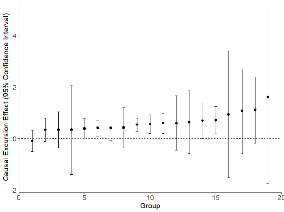
The Intern Health Study (IHS) is a 6-month MRT on 1,562 medical interns [10]. Due to high depression rates and levels of stress during the first year of physician residency training, a critical question is whether targeted notifications can improve mood, increase sleep time, and/or increase physical activity. Enrolled medical interns were randomized weekly to receive either mood, activity, or sleep notifications or receive no notifications for that week (probability 1/4 each). Analyses conducted in this paper focus on the weekly randomization; see [10] for further study details. Figure 1 presents specialty-specific effect estimates on weekly average mood scores using (3), with evident specialty-level treatment effect heterogeneity. This suggests a marginal analysis must account for effect heterogeneity at the specialty-level. The present work offers such a framework to address the inferential deficiency that we show if the standard WCLS were used under cluster-level effect heterogeneity. In addition, there exists potential within-cluster interference of other subjects’ treatments upon a subject’s outcome. Our framework defines a new and useful indirect excursion effect under sequential treatments in contrast to existing work that mostly focuses on indirect effects in non-temporal settings.
3. Cluster-Level Proximal Treatment Effects
3.1. Proximal Moderated Treatment Effects: A Cluster-based Conceptualization
Consider a cluster of size . Overbar will continue to denote treatment sequences; , for instance, denotes the sequence of realized treatment sequence up to and including decision time for individual . Let denote the set of realized treatments for all individuals in the cluster. Let denote this set with the th individual removed. Let denote the potential outcome for individual which may depend on realized treatments for all subjects in the cluster.
Direct causal excursion effects. In standard MRTs, the individual is the unit of interest. Here, the cluster is the unit of interest and the effect of interest is in providing treatment versus not providing treatment at time on a random individual in the group. This can be expressed as a difference in potential outcomes for the proximal response
| (4) |
Following [11] and [12], (4) is a group average direct causal effect of treatment versus no treatment fixing all other treatments.
The “fundamental problem of causal inference” [7, 13] is that individual differences cannot be observed. Thus, similar to prior work [5, 3], averages of potential outcomes are considered. Let denote a vector of potential moderator variables formed from , the cluster-level history up to decision point . Then the moderated direct treatment effect, denoted , can be defined as
| (5) |
where is a uniformly distributed random index defined on . The expectation is over the potential outcomes , the randomized treatments – , , and – and the random index . Choice of depends on the scientific question of interest. A primary analysis may focus on marginal effects and set . A second analysis may focus on assessing the effect conditional on variables only related to the individual indexed by and set , i.e., a potential individual-level moderator of interest where produces a vector of summary variables from the history of individual , . A third analysis may consider group-level moderators such as or . Equation (5) generalizes the population average direct causal effect from [12] to a group-level causal excursion effect that allows for moderation and time-varying treatments.
Pairwise indirect causal excursion effects. Of secondary interest is the indirect effect of providing treatment versus not providing treatment to the th individual at time on a different individual’s proximal response, i.e., pairwise within-cluster treatment interference. Here, we define the pairwise indirect causal excursion effect as
Again, since individual differences cannot be observed, averages of potential outcomes are considered. The moderated pairwise indirect treatment effect, denoted , is
| (6) |
where is uniformly distributed random index on the set . The expectation is over both the potential outcomes , randomized treatments – , , , , and – and the random indices ( and ). The potential moderator can be written as to clarify that the variables can contain both information on the two selected individuals as well as others in the cluster. Another pairwise indirect effect can be defined when individual receives treatment, i.e., instead of as in (6).
Remark 3.1.
The effect defined by (6) generalizes the group average indirect causal effect from [12] to a group-level pairwise indirect causal excursion effect that allows for moderation and time-varying treatments. To see this, note that the excursion effect at each decision time averages over a particular reference distribution over the past and future treatments up to and including time defined by the MRT randomization probabilities and the alternative probability distribution . The contrast is over two treatment allocations, both where a random individual does not receive treatment, but where in one allocation another random individual receives treatment and in the other allocation that same individual does not receive treatment. [12] consider contrasts between any two randomized treatment allocations conditional on a random individual not receiving treatment in a non-temporal setting. Therefore, per decision time our definition is a special case of their indirect effect where, for a random non-treated individual, we focus on treating or not treating another random individual and marginalizing over all others in the group. More complex contrasts could be derived such as three- or four-way indirect effects; however, the number of combinations grows quickly making estimation unrealistic in our setting. Our choice of contrast was thus motivated by finding an estimand of scientific interest which could be reasonably estimated within the MRT setting, bridging the literature on causal excursions and indirect effects.
3.2. Causal Excursion Effect Estimand Depends on Treatment Distribution
Estimands considered here are most similar to average outcomes under a particular dynamic treatment regime where denotes the dynamic treatment regime from which the treatments are drawn [14]. Indeed, for any not contained in , the direct and indirect effects depend on the distribution of . Estimands (5) and (6) marginalize over treatments not contained in . Marginalization over different probabilistic assignment of treatments may yield different results. Therefore, the direct and indirect excursion effects depend on the study protocol and choice of alternative distribution . The reason for this is that micro-randomization is meant to gather information on how to optimize the design of intervention components [15]. The marginal formulation of main and moderation effects contrasts excursions from the current treatment protocol, and mimics analyses used in a factorial design that marginalize over factors including time. See [4, Section 8] for additional considerations. Regardless, the effects considered in this paper are causal and depend on the treatment assignment distributions. Due to this dependence, in real data analysis, we recommend presenting the micro-randomization distribution together with the estimated treatment effects, thus the subscript in the definition of both the direct and indirect effects are specified.
3.3. Identification
Causal effects (5) and (6) can be expressed in terms of the observable data under the following standard set of causal inference assumptions [8]:
Assumption 3.2.
We assume consistency, positivity, and sequential ignorability:
-
•
Consistency: For each and , , i.e., observed values equal the corresponding potential outcomes;
-
•
Positivity: if the joint density is greater than zero, then ;
-
•
Sequential ignorability: for each , the potential outcomes,
, are independent of conditional on the observed history .
Sequential ignorability and, assuming all of the randomization probabilities are bounded away from and , positivity, are guaranteed in our setting by design. Consistency is a necessary assumption for linking the potential outcomes as defined here to the data. Since an individual’s outcomes may be influenced by the treatments provided to other individuals in the same cluster, consistency holds due to our use of a cluster-based conceptualization of potential outcomes as seen in [16] and [17].
Lemma 3.3.
Under Assumption 3.2, the moderated direct treatment effect is equal to
where expectations are with respect to the distribution of the data collected under the actual treatment assignment probabilities , and with ; and the moderated indirect treatment effect is equal to
where with .
4. Estimation
4.1. Direct Causal Excursion Effect Estimation
Assumption 4.1.
Assume the direct causal excursion effect where is a -dimensional feature vector that is a function of moderator state and decision point .
Consider inference on the -dimensional parameter . Define the weight at decision time for the th individual as equal to where is arbitrary as long as it does not depend on terms in other than , and is the marginal probability that individual receives treatment given . Here we consider an estimator which is the minimizer of a cluster-based, weighted-centered least-squares (C-WCLS) criterion:
| (7) |
where is defined as the average of a function over the sample, which in this context is the sample of clusters rather than the sample of individuals as in traditional MRT settings. In Appendix B, we prove the following result.
Lemma 4.2.
In practice, plug-in estimates and are used to estimate the covariance structure; Appendix F presents their estimates with small-sample adjustments.
Remark 4.3.
( Projection Interpretation) Importantly, Assumption 4.1 is not required. That is, we can follow [18, 19, 20, 5] and others in using as a working model for . Specifically, is a solution to the weighted least-squares projection
Here, the weight is the variance of the numerator in the weight . To interpret as a projection or as a correctly specified causal effect can be viewed as a bias-variance trade-off. The projection interpretation guarantees well-defined parameter interpretation in practice where Assumption 4.1 is unlikely to hold. See [Sec. 3.1, pp.9–10 20] for a discussion of the use of projections in causal versus predictive settings.
Appendix I presents semiparametric efficiency theory in the special case of .
4.2. Connection to the Standard MRT Analysis
A natural question is whether there are conditions such that the standard MRT analysis presented in Section 2.2 is equivalent to the proposed direct effect analysis. Lemma 4.4 proves that, under certain conditions, an equivalence of estimates and asymptotic variances is guaranteed.
Lemma 4.4.
Consider the direct effect when the moderator is defined on the individual (i.e., ), and the randomization probabilities only depend on the individual’s observed history, i.e., . If cluster size is constant (i.e., ), then the point estimates from (3) and (5) are equal for any sample size. Moreover, if
| (8) |
equals for some function , i.e., the cross-terms are constant in and , where is the error defined in Lemma 4.2, then the estimators share the same asymptotic variance.
Proof of Lemma 4.4 can be found in Appendix E. Here, a class of random effect models is introduced to help with interpretation of the sufficient condition (8). Specifically, for participant at decision time , let and suppose the generative model for the proximal response is
where and are random effects with design matrix , , and is a participant-specific error term. The treatment effect conditional on the complete observed history and the random effects is , which implies the marginal causal effect is so Assumption 4.1 holds. Random effects in allow for cluster-level variation in baseline values of the proximal response, while random effects in allow for cluster-level variation in the fully-conditional treatment effect. Given the above generative model, sufficient condition (8) holds if , i.e., when the treatment effect does not exhibit cluster-level variation. For this reason, (8) is referred to as a treatment-effect heterogeneity condition. The condition motivates our simulation study in Section 5, which empirically supports this conclusion of equivalence.
4.3. Pairwise Indirect Causal Excursion Effect Estimation
Assumption 4.5.
Assume the pairwise indirect causal excursion effect , where is a -dimensional vector function of and time .
Consider inference on the -dimensional parameter . Define the weight at decision time for the th individual as equal to where is arbitrary as long as it does not depend on terms in other than , and is the marginal probability that individuals and receive treatments and respectively given . Here we consider an estimator which is the minimizer of the following cluster-based weighted-centered least-squares (C-WCLS) criterion:
| (9) |
where and . If an individual’s randomization probabilities only depends on their own observed history then and the weight . In Appendix A, we prove the following result.
Lemma 4.6.
Remark 4.7.
In Appendix H, variances are re-derived in the general setting where the numerators and are estimated using the observed MRT data.
5. Simulations
To evaluate the proposed estimator, we extend the simulation setup in [3]. We first present a base data generation model, which is to be extended in four scenarios. In this section, we focus on presenting simulation settings and results for lag-1 proximal responses (); see Appendix D for scenarios under with similar conclusions about the relative advantage of the proposed method. Consider an MRT with known randomization probability and the observation vector being a single state variable at each decision time . Let
| (10) |
The randomization probability is where ; the state dynamics are given by with , and the independent error term satisfies with . As in [3], we set , and . Because , the marginal proximal effect is equal to . In extending the data generation model to clustered settings, we conducted simulation studies with clusters with equal sizes ( or ); here, we report results with clusters showing the relative advantage of C-WCLS over WCLS. A more complete set of simulation results with similar findings can be found in Appendix C.
Simulation Scenario I. The first scenario estimates the marginal proximal effect when an individual-level moderator exists and proximal responses share a random cluster-level intercept term that does not interact with treatment. The data generative model (10) incorporates a cluster-level random-intercept . Table 1 presents the results, which shows both WCLS and the proposed C-WCLS approach are nearly unbiased and have proper coverage rates. This is in line with Lemma 4.4 stating asymptotic equivalence under no cluster-level treatment heterogeneity.
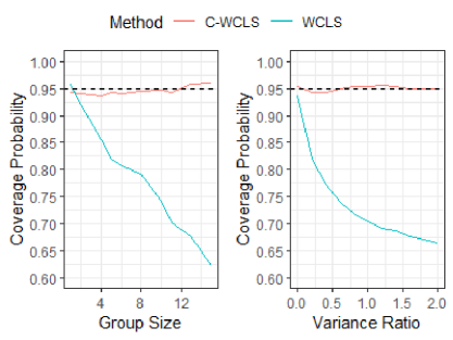
Simulation Scenario II. In the second scenario, we extend Scenario I to include a random cluster-level intercept term that interacts with treatment by considering the linear model with the additional term where . Table 1 presents the results which demonstrate that if cluster-level random effects interact with treatment, then both methods produce nearly unbiased estimates of the marginal proximal effect but only the proposed method achieves the nominal 95% coverage probability. To further demonstrate this, Figure 2 presents nominal coverage as a function of the ratio of the variance of over the variance of as well as group size respectively.
Simulation Scenario III. In the third scenario, the treatment effect for an individual is assumed to depend on the average state of all individuals in the cluster, i.e., define the cluster-level moderator and consider the linear model from Scenario II with the additional term . The proposed estimator again achieves the nominal 95% coverage probability while the WCLS method does not (see Scenario III, Table 1).
| Scenario | Estimator | # of Clusters | Cluster Size | Estimate | SE | RMSE | CP |
|---|---|---|---|---|---|---|---|
| I | C-WCLS | 50 | 10 | -0.198 | 0.025 | 0.027 | 0.935 |
| WCLS | -0.198 | 0.026 | 0.026 | 0.944 | |||
| C-WCLS | 50 | 25 | -0.198 | 0.016 | 0.016 | 0.950 | |
| WCLS | -0.198 | 0.016 | 0.017 | 0.937 | |||
| II | C-WCLS | 50 | 10 | -0.200 | 0.051 | 0.049 | 0.957 |
| WCLS | -0.200 | 0.029 | 0.052 | 0.723 | |||
| C-WCLS | 50 | 25 | -0.200 | 0.047 | 0.049 | 0.947 | |
| WCLS | -0.199 | 0.019 | 0.048 | 0.555 | |||
| III | C-WCLS | 50 | 10 | -0.198 | 0.051 | 0.052 | 0.941 |
| WCLS | -0.199 | 0.029 | 0.052 | 0.742 | |||
| C-WCLS | 50 | 25 | -0.199 | 0.047 | 0.048 | 0.946 | |
| WCLS | -0.200 | 0.018 | 0.048 | 0.561 | |||
| IV | C-WCLS | 50 | 10 | -0.097 | 0.020 | 0.021 | 0.953 |
| 25 | -0.100 | 0.013 | 0.013 | 0.942 |
Simulation Scenario IV. The fourth scenario considers the indirect effect. For individual at decision point , define the total effect to be , where and . The generative model is then given by:
This model implies a marginal pairwise indirect effect equal to . Table 1 presents simulation results which shows that the proposed indirect estimator exhibited nearly no bias and achieved the nominal coverage probability.
6. Case Study: Intern Health Study
The Intern Health Study (IHS) was a 6-month MRT on 1,562 medical interns where four types of weekly notification - mood, activity, sleep, or none – were randomly assigned with equal probability to each subject [10]; see Section 2.3 for prior discussion. In IHS, 285 institutions and 24 specialties were observed. Here, we assess the effect of the three types of notifications (mood, activity, and sleep) compared to no notifications on the weekly average of self-reported mood scores, log step-count and log sleep minutes for the population of interns. Due to high levels of missing data, weekly proximal responses were multiply imputed. See [10] for further details.
Let denote the weekly decision points at which the individual is randomized to the various types of notifications. The three proximal responses are the average weekly mood score, which is reported on a Likert scale taking values from 1 to 10 (higher scores mean better mood), log step count and log sleep minutes respectively. Notifications are collapsed to a binary variable, i.e., if the individual was assigned to receive any notifications on week ; otherwise, . We start by defining clusters based on medical specialty as we saw effect heterogeneity by specialty in Figure 1. The average cluster size was 65; the first and third quartile were 7 and 113 respectively, with maximum and minimum sizes of 333 and 1. For every individual in each cluster at each decision point, we compute the average prior weekly proximal response for all others in the cluster, denoted for the th individual in the cluster. We conducted analyses under lag and . Here we report results under ; see Appendix G for results under for two choices of reference policy . Under , we consider two moderation analyses that can both be expressed as .
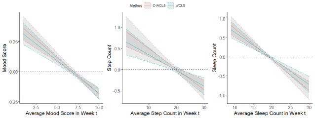
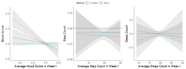
The first set of moderation analyses considers the standard moderation analysis where only individual-level moderators are included (i.e., ). Figure 3 visualizes the estimates across the range of prior week’s proximal response for both our proposed approach and the WCLS approach from [3], and the numerical output can be found in Appendix G.1. In comparison, C-WCLS produces larger variance estimates for all proximal responses as expected. The effects do not change too much for the average weekly mood and sleep analysis; however, the significant effect of messages on weekly log step count under the traditional MRT analysis becomes insignificant when accounting for cluster effects.
The second moderation analysis lets be a free parameter, enabling novel moderation analyses that accounts for the average weekly previous proximal responses of other individuals. Table 2 presents the results. Here, we see that the new term is negative but insignificant. The results suggest the average proximal responses of others in the cluster have a limited moderation effect. To conclude, the impact of a notification on mood is larger while the individual’s score from previous week is low. Similar results hold for the log step-count analysis.
| Direct Effect | Indirect Effect | |||||||
|---|---|---|---|---|---|---|---|---|
| Variables | Estimate | Std. Error | p-value | Variables | Estimate | Std. Error | p-value | |
| Mood | Intercept () | 0.563 | 0.251 | 0.028 | -0.054 | 0.045 | 0.883 | |
| Prior Week Avg. () | -0.066 | 0.027 | 0.016 | -0.015 | 0.031 | 0.684 | ||
| Cluster Pr. Wk. Avg. () | -0.016 | 0.017 | 0.349 | |||||
| Steps | Intercept () | 1.165 | 0.782 | 0.139 | -0.038 | 0.134 | 0.612 | |
| Prior Week Avg. () | -0.048 | 0.036 | 0.177 | 0.019 | 0.090 | 0.417 | ||
| Cluster Pr. Wk. Avg. () | -0.010 | 0.014 | 0.482 | |||||
| Sleep | Intercept () | 1.545 | 0.779 | 0.050 | 0.007 | 0.096 | 0.469 | |
| Prior Week Avg. () | -0.081 | 0.039 | 0.037 | -0.004 | 0.065 | 0.526 | ||
| Cluster Pr. Wk. Avg. () | 0.000 | 0.006 | 0.961 | |||||
Finally, we consider indirect moderation effect analyses. In this analysis, clusters are defined based on medical specialty and institution because interference was only likely when interns are in close geographic proximity. Here, we consider the marginal indirect effect (e.g., no moderators) both when the individual did not receive the intervention and when the individual did receive an intervention at decision time . Table 2 presents the results. In this case, the estimated indirect effects are much weaker than the direct effects. Even a weak effect may be unexpected as none of the content in the push notifications was aimed at impacting other individuals’ behavior. For all the proximal responses, we see limited evidence of an indirect effect. This implies that the scientific team, when building an optimal intervention package, may ignore these indirect effects and focus solely on the individual who receives these types of push notifications.
7. Discussion
We revisited causal excursion effects in the presence of a priori known clusters in sequential treatment settings where outcome of interest is measured at all decision points. In particular, we formalized both direct and indirect excursion effects in the context of MRT to account for potential interference. We studied their identifications and proposed consistent and robust inference methods. In practice, the effects described in this paper are most important when using MRT data to build optimized just-in-time adaptive interventions (JITAIs) for deployment in an mHealth package. Specifically, the estimation procedure for the direct excursion effect accounts for within-cluster correlation in the proximal responses which helps the scientific team avoid making erroneous conclusions about intervention effectiveness using standard MRT methods. Moreover, estimation of indirect effects allows the scientific team to answer questions about impact of interventions on other members of the same cluster. Use of these methods provides empirical evidence for the scientific team to include or exclude intervention components that may have had unanticipated second order effects, or potentially lead to novel ways to improve the intervention component by revising the intervention to more explicitly account for cluster-level interference. While this work represents a major step forward in the analysis of micro-randomized trial data, further work is required. Specifically, useful extensions include accounting for overlapping communities and/or network (rather than cluster-only) structure [21, 22], accounting for general non-continuous proximal responses such as binary or count outcomes [4], penalization of the working model to allow for high-dimensional moderators, and a method to use the proposed approach to form warm-start policies at the individual level while accounting for group level information [23].
References
- [1] I. Nahum-Shani, S.N. Smith, B.J. Spring, L.M. Collins, K. Witkiewitz, A. Tewari, and S.A. Murphy. Just-in-time adaptive interventions (JITAIs) in mobile health: Key components and design principles for ongoing health behavior support. Annals of Behavioral Medicine, 2017.
- [2] P. Klasnja, E.B. Hekler, S. Shiffman, A. Boruvka, D. Almirall, A. Tewari, and S.A. Murphy. Microrandomized trials: An experimental design for developing just-in-time adaptive interventions. Health Psychol, 34:1220–1228, 2015.
- [3] Audrey Boruvka, Daniel Almirall, Katie Witkiewitz, and Susan A. Murphy. Assessing time-varying causal effect moderation in mobile health. Journal of the American Statistical Association, 113(523):1112–1121, 2018.
- [4] Tianchen Qian, Hyesun Yoo, Predrag Klasnja, Daniel Almirall, and Susan Murphy. Estimating time-varying causal excursion effect in mobile health with binary outcomes. Biometrika, 09 2020. asaa070.
- [5] W. Dempsey, P. Liao, and S.A. Murphy. The stratified micro-randomized trial design: Sample size considerations for testing nested causal effects of time-varying treatments. Annals of Applied Statistics, 14(2):661–684, 2020.
- [6] P. Liao, P. Klasjna, A. Tewari, and S.A. Murphy. Micro-randomized trials in mhealth. Statistics in Medicine, 35(12):1944–71, 2016.
- [7] DB. Rubin. Bayesian inference for causal effects: The role of randomization. The Annals of Statistics, 6(1):34–58, 1978.
- [8] J. Robins. A new approach to causal inference in mortality studies with a sustained exposure period-application to control of the healthy worker survivor effect. Mathematical Modelling, 7(9):1393–1512, 1986.
- [9] KY Liang and SL Zeger. Longitudinal data analysis using generalized linear models. Biometrika, 73(1):13–22, 1986.
- [10] Timothy NeCamp, Srijan Sen, Elena Frank, Maureen A Walton, Edward L Ionides, Yu Fang, Ambuj Tewari, and Zhenke Wu. Assessing real-time moderation for developing adaptive mobile health interventions for medical interns: Micro-randomized trial. Journal of medical Internet research, 22(3):e15033, March 2020.
- [11] ME Halloran and CJ Struchiner. Causal inference for infectious diseases. Epidemiology, 6:142–151, 1995.
- [12] E. J. Tchetgen Tchetgen, M.M. Glymour, J. Weuve, and Robins J. Specifying the correlation structure in inverse-probability-weighting estimation for repeated measures. Epidemiology, 23(4):644–646, 2012.
- [13] J. Pearl. Causal inference in statistics: An overview. Statistics Surveys, 3:96–146, 2009.
- [14] S A Murphy, M J van der Laan, J M Robins, and Conduct Problems Prevention Research Group. Marginal mean models for dynamic regimes. Journal of the American Statistical Association, 96(456):1410–1423, 2001. PMID: 20019887.
- [15] L.M. Collins. Optimization of Behavioral, Biobehavioral, and Biomedical Interventions. Springer International Publishing, 2018.
- [16] G. Hong and S. W. Raudenbush. Evaluating kindergarten retention policy. Journal of the American Statistical Association, 101(475):901–910, 2006.
- [17] T. J. Vanderweele, G. Hong, S.M. Jones, and J.L. Brown. Mediation and spillover effects in group-randomized trials: A case study of the 4Rs educational intervention. Journal of the American Statistical Association, 108(502):469–482, 2013.
- [18] R. Neugebauer and M. J. van der Laan. Nonparametric causal effects based on marginal structural models. Journal of Statistical Planning and Inference, 137:419–434, 2007.
- [19] M. A. Rosenblum and M. J. van der Laan. Targeted maximum likelihood estimation of the parameter of a marginal structural model. The International Journal of Biostatistics, 6, 2010.
- [20] Edward H. Kennedy, Scott Lorch, and Dylan S. Small. Robust causal inference with continuous instruments using the local instrumental variable curve. Journal of the Royal Statistical Society: Series B (Statistical Methodology), 81(1):121–143, 2019.
- [21] E. Ogburn and T. VanderWeele. Causal diagrams for interference. Statistical Science, 29(4):559–578, 2014.
- [22] Georgia Papadogeorgou, Fabrizia Mealli, and Corwin M. Zigler. Causal inference with interfering units for cluster and population level treatment allocation programs. Biometrics, 75(3):778–787, 2019.
- [23] Daniel J. Luckett, Eric B. Laber, Anna R. Kahkoska, David M. Maahs, Elizabeth Mayer-Davis, and Michael R. Kosorok. Estimating dynamic treatment regimes in mobile health using v-learning. Journal of the American Statistical Association, 115(530):692–706, 2020. PMID: 32952236.
- [24] LA. Mancl and T.A. DeRouen. A covariance estimator for GEE with improved small-sample properties. Biometrics, 57(1):126–134, 2001.
- [25] J. M. Robins. Correcting for non-compliance in randomized trials using structural nested mean models. Communications in Statistics-Theory and Methods, 23:2379–2412, 1994.
- [26] W.K. Newey. Semiparametric efficiency bounds. Journal of Applied Econometrics, (5):99–135, 1990.
- [27] A. Tsiatis. Semiparametric Theory and Missing Data. Springer Science & Business Media, 2007.
Appendix A Technical Details
Lemma 3.3.
We establish Lemma 3.3 for the direct effect (5). For , we consider
since the history includes the moderator variable at time . By consistency, . Moreover, sequential ignorability implies that
It also implies that . Summing over all potential outcomes yields
Averaging over individuals in the group group size completes the proof. The proof for the indirect effect follows the exact same structure. ∎
Appendix B Lemma 4.2
We next provide a detailed proof of asymptotic normality and consistency for the weighted-centered least squares estimator.
Consistency for direct and indirect effects.
The solutions that minimize equation (7) are consistent estimators for the solutions that minimize the following
Differentiating the above equation with respect to yields a set of estimating equations.
We note that
Therefore, we have,
We note that
Now differentiating with respect to yields
Then we have
Under assumption 4.1, we have that which guarantees consistency.
We next consider the indirect effect estimator. Recall that
is the replacement for in the direct effect for centering. If we make the assumption that then ; however, we provide the proof in complete generality. The estimates that minimize equation (9) are consistent estimators for the solutions that minimize the following
Differentiating the above equation with respect to yields a set of estimating equations.
We note that
Therefore, we have,
First, we show that
and
This implies that
Now differentiating with respect to yields
Under assumption 4.5, we have that which guarantees consistency. ∎
Asymptotic Normality.
We now consider the issue of asymptotic normality. First, let
, and . Since define . Then
By definitions of and and the previous consistency argument
Then under moments conditions, we have asymptotic normality with variance given by
Due to centering, the expectation of the matrix is block diagonal and the sub-covariance matrix can be extracted and is equal to
The outer terms are equal to , which gives us the covariance as desired.
We next consider asymptotic normality in the indirect setting. First, let
, and . Since define . Then equals
By definitions of and and the previous consistency argument
Then under moments conditions, we have asymptotic normality with variance given by
Due to centering, the expectation of the matrix is block diagonal and the sub-covariance matrix can be extracted and is equal to
as desired. ∎
Appendix C Additional simulation details
| Scenario | Estimator | # of Clusters | Cluster Size | Estimate | SE | RMSE | CP |
|---|---|---|---|---|---|---|---|
| I | C-WCLS | 25 | 10 | -0.198 | 0.035 | 0.036 | 0.945 |
| WCLS | -0.200 | 0.036 | 0.035 | 0.956 | |||
| C-WCLS | 25 | 25 | -0.199 | 0.022 | 0.023 | 0.948 | |
| WCLS | -0.199 | 0.023 | 0.022 | 0.958 | |||
| C-WCLS | 50 | 10 | -0.198 | 0.025 | 0.027 | 0.935 | |
| WCLS | -0.198 | 0.026 | 0.026 | 0.944 | |||
| C-WCLS | 50 | 25 | -0.198 | 0.016 | 0.016 | 0.950 | |
| WCLS | -0.198 | 0.016 | 0.017 | 0.937 | |||
| C-WCLS | 100 | 10 | -0.199 | 0.018 | 0.018 | 0.949 | |
| WCLS | -0.198 | 0.018 | 0.019 | 0.949 | |||
| C-WCLS | 100 | 25 | -0.198 | 0.011 | 0.012 | 0.941 | |
| WCLS | -0.199 | 0.011 | 0.012 | 0.944 | |||
| II | C-WCLS | 25 | 10 | -0.199 | 0.070 | 0.076 | 0.935 |
| WCLS | -0.201 | 0.041 | 0.076 | 0.710 | |||
| C-WCLS | 25 | 25 | -0.196 | 0.065 | 0.071 | 0.933 | |
| WCLS | -0.200 | 0.026 | 0.065 | 0.557 | |||
| C-WCLS | 50 | 10 | -0.200 | 0.051 | 0.049 | 0.957 | |
| WCLS | -0.200 | 0.029 | 0.052 | 0.723 | |||
| C-WCLS | 50 | 25 | -0.200 | 0.047 | 0.049 | 0.947 | |
| WCLS | -0.199 | 0.019 | 0.048 | 0.555 | |||
| C-WCLS | 100 | 10 | -0.198 | 0.036 | 0.035 | 0.955 | |
| WCLS | -0.198 | 0.021 | 0.037 | 0.718 | |||
| C-WCLS | 100 | 25 | -0.198 | 0.033 | 0.035 | 0.942 | |
| WCLS | -0.199 | 0.013 | 0.032 | 0.583 | |||
| III | C-WCLS | 25 | 10 | -0.199 | 0.070 | 0.073 | 0.948 |
| WCLS | -0.202 | 0.041 | 0.074 | 0.734 | |||
| C-WCLS | 25 | 25 | -0.196 | 0.066 | 0.069 | 0.931 | |
| WCLS | -0.200 | 0.026 | 0.068 | 0.563 | |||
| C-WCLS | 50 | 10 | -0.198 | 0.051 | 0.052 | 0.941 | |
| WCLS | -0.199 | 0.029 | 0.052 | 0.742 | |||
| C-WCLS | 50 | 25 | -0.199 | 0.047 | 0.048 | 0.946 | |
| WCLS | -0.200 | 0.018 | 0.048 | 0.561 | |||
| C-WCLS | 100 | 10 | -0.200 | 0.036 | 0.037 | 0.946 | |
| WCLS | -0.200 | 0.021 | 0.037 | 0.740 | |||
| C-WCLS | 100 | 25 | -0.201 | 0.034 | 0.033 | 0.956 | |
| WCLS | -0.198 | 0.013 | 0.034 | 0.555 |
| Scenario | # of Clusters | Cluster Size | Estimate | SD | RMSE | CP |
|---|---|---|---|---|---|---|
| IV | 25 | 10 | -0.097 | 0.028 | 0.029 | 0.958 |
| 25 | 25 | -0.101 | 0.017 | 0.019 | 0.942 | |
| 50 | 10 | -0.097 | 0.020 | 0.021 | 0.953 | |
| 50 | 25 | -0.100 | 0.013 | 0.013 | 0.942 | |
| 100 | 10 | -0.097 | 0.015 | 0.015 | 0.943 | |
| 100 | 25 | -0.100 | 0.009 | 0.009 | 0.944 |
Appendix D Simulation for Lag Effect estimation
D.1. Simulation setup
To evaluate the proposed estimator with , we extend the simulation setup in the main paper. Consider an MRT with the same setting, in addition to and , thus, and the proximal response is:
| (11) |
Here we identify two prespecified future (after time t) ”reference” treatment regimes that define the distribution for . The first one assigns treatment with probabilities between zero and one and corresponds to the treatment assignment distribution, and the second one chooses the reference regime for , with probability one. In this case, the lag treatment effect represents the impact of a sequential treatments on the proximal response time units later.
Simulation Scenario I. The first scenario estimates when an individual-level moderator exists and proximal responses share a random cluster-level intercept term that does not interact with treatment. The data generative model (11) incorporates a cluster-level random-intercept . Table 5 presents the results, which shows under both future treatment policies, the proposed C-WCLS approach achieve nearly unbiasedness and proper coverage.
Simulation Scenario II. In the second scenario, we extend scenario I to include a random cluster-level intercept term that interacts with the treatment by considering the linear model with the additional term where . Table 5 presents the results which demonstrate that if cluster-level random effects interact with the previous treatment, then both policies produce nearly unbiased estimates and the proposed method achieves the nominal 95% coverage probability.
Simulation Scenario III. In the third scenario, the lag treatment effect for an individual is assumed to depend on the average state of all individuals in the cluster, i.e., define the cluster-level moderator and consider the linear model from Scenario II with the additional term . The proposed estimator again achieves the nominal 95% coverage probability (see Scenario III, Table 5).
D.2. Lag Treatment Effect Calculation
Sequential Treatment Regime. As stated by the sequential treatment reference regime, we have the weight . Thus, the true lag treatment effect can simply be calculated as:
| (12) |
Under our simulation setting, the term is equal to:
Splitting the expectation above to three terms, we have the following calculation:
| (13) |
| (14) |
| (15) |
Therefore,
and the true lag treatment effect under sequential treatment regime is equal to:
| (16) |
Observed Distribution Treatment Regime. As specified by this reference treatment regime, we have future treatment reference distribution the same with the distribution of treatments in the data we have at hand, i.e., and . Thus, the true lag treatment effect can be calculated as:
| (17) |
Similar as above, under our simulation setting, the term is equal to:
The three terms are calculated below:
| (18) |
| (19) |
| (20) |
Therefore,
and the true lag treatment effect under observed treatment distribution regime is equal to:
| (21) |
D.3. Marginal Lag Treatment Effect Simulation Results
The choice for prespecified future reference treatment regimes is of vital importance and often time yields to different treatment effect estimations. Following the derivations above, the fully marginal lag treatment effect is -0.128 for sequential treatment reference regime, and -0.1 for observed treatment distribution regime. Table 5 presents the simulation results.
| Scenario | Policy | # of Clusters | Cluster Size | Estimate | SE | RMSE | CP |
|---|---|---|---|---|---|---|---|
| I | OTD | 50 | 10 | -0.098 | 0.031 | 0.032 | 0.938 |
| ST | -0.123 | 0.062 | 0.063 | 0.949 | |||
| OTD | 50 | 25 | -0.098 | 0.020 | 0.020 | 0.948 | |
| ST | -0.124 | 0.040 | 0.039 | 0.955 | |||
| II | OTD | 50 | 10 | -0.099 | 0.054 | 0.054 | 0.944 |
| ST | -0.122 | 0.077 | 0.078 | 0.949 | |||
| OTD | 50 | 25 | -0.099 | 0.048 | 0.049 | 0.942 | |
| ST | -0.121 | 0.059 | 0.061 | 0.950 | |||
| III | OTD | 50 | 10 | -0.096 | 0.054 | 0.056 | 0.942 |
| ST | -0.122 | 0.075 | 0.075 | 0.948 | |||
| OTD | 50 | 25 | -0.099 | 0.048 | 0.050 | 0.944 | |
| ST | -0.125 | 0.059 | 0.059 | 0.955 |
Appendix E Proof of Lemma 4.4
Proof.
Consider the -matrix for the direct effect asymptotic variance,
Consider the cross-terms with and without loss of generality assume , then
Under the assumption of the error cross-term being constant in and we can re-write the above as:
Therefore, we have that the -matrix simplifies to
which is the matrix as in the standard MRT analysis. ∎
Appendix F Small sample size adjustment for covariance estimation
The robust sandwich covariance estimator [24] for the entire variance matrix is given by . The first term, , is given by
where is the model matrix for individual in group associated with equation (7), and is a diagonal matrix of individual weights. The middle term is given by
where is an identity matrix of correct dimension, is the individual-specific residual vector and
From we extract .
Appendix G Additional analysis of IHS
G.1. Additional Information for Figure 3
Figure 3 presented a visually comparison between WCLS and C-WCLS in terms of the moderation of average previous week’s proximal outcomes on the effect of notifications on average weekly mood scores, log step counts, and log sleep counts respectively in IHS. Here we attach the table for numerical comparison.
| Outcome | Setting | Variables | Estimate | Std. Error | t-value | p-value |
|---|---|---|---|---|---|---|
| Mood | WCLS | 0.369 | 0.086 | 4.267 | 0.000 | |
| -0.055 | 0.011 | -4.822 | 0.000 | |||
| C-WCLS | 0.421 | 0.214 | 1.968 | 0.053 | ||
| -0.061 | 0.028 | -2.181 | 0.032 | |||
| Steps | WCLS | 0.729 | 0.295 | 2.472 | 0.015 | |
| -0.037 | 0.015 | -2.484 | 0.015 | |||
| C-WCLS | 0.997 | 0.734 | 1.357 | 0.176 | ||
| -0.049 | 0.037 | -1.343 | 0.181 | |||
| Sleep | WCLS | 1.325 | 0.350 | 3.782 | 0.000 | |
| -0.068 | 0.017 | -3.916 | 0.000 | |||
| C-WCLS | 1.543 | 0.767 | 2.012 | 0.046 | ||
| -0.081 | 0.039 | -2.082 | 0.039 |
G.2. Lagged Treatment Effect
We implement an extended investigation on the lag treatment effect of the targeted mobile notifications. The same two models: are applied to moderation analyses.
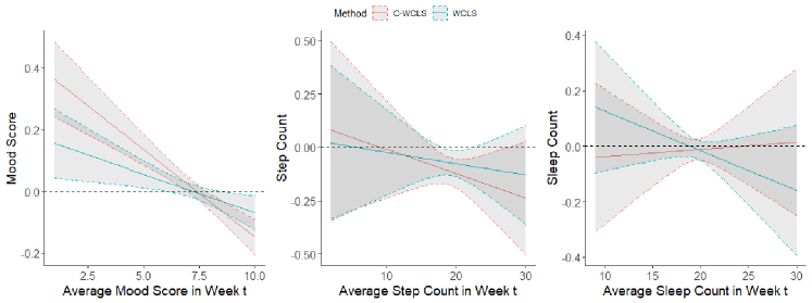
The first set of moderation analyses considers the standard moderation analysis where only individual-level moderators are included (i.e., ), with or without accounting for cluster-level moderation effect heterogeneity. Figure 4 and Figure 5 visualize the estimates across the range of prior week’s proximal response for both our proposed approach and the WCLS approach from [3]. In this case, the effects do not change too much for all the analysis;
The second moderation analysis lets be a free parameter. Table 7 and Table 8 present the results. Here, we see that the constant term in the mood analysis becomes significant, while the new term is insignificant. The results suggest the average proximal outcomes of others in the cluster have a limited moderate effect on notifications, however, the lag impact of a notification on mood is positive and significant.
| Outcome | Setting | Variables | Estimate | Std. Error | t-value | p-value |
|---|---|---|---|---|---|---|
| Mood | C-WCLS | 0.665 | 0.321 | 2.072 | 0.040 | |
| -0.067 | 0.037 | -1.804 | 0.072 | |||
| -0.027 | 0.019 | -1.393 | 0.164 | |||
| Steps | C-WCLS | 0.234 | 1.039 | 0.225 | 0.823 | |
| -0.011 | 0.045 | -0.254 | 0.800 | |||
| -0.007 | 0.021 | -0.354 | 0.725 | |||
| Sleep | C-WCLS | -0.073 | 0.887 | -0.082 | 0.935 | |
| 0.002 | 0.043 | 0.049 | 0.961 | |||
| 0.001 | 0.008 | 0.135 | 0.893 |
| Outcome | Setting | Variables | Estimate | Std. Error | t-value | p-value |
|---|---|---|---|---|---|---|
| Mood | C-WCLS | 0.585 | 0.292 | 2.002 | 0.046 | |
| -0.061 | 0.036 | -1.702 | 0.090 | |||
| -0.022 | 0.021 | -1.038 | 0.299 | |||
| Steps | C-WCLS | 0.107 | 0.951 | 0.113 | 0.911 | |
| -0.001 | 0.041 | -0.033 | 0.974 | |||
| -0.011 | 0.018 | -0.629 | 0.531 | |||
| Sleep | C-WCLS | -0.211 | 0.802 | -0.263 | 0.793 | |
| 0.009 | 0.040 | 0.233 | 0.816 | |||
| 0.001 | 0.007 | 0.193 | 0.848 |
Appendix H Additional details on the indirect effect
Weights used in the estimation of the indirect effect is a natural extension of [3]. As in Section 4.3, the weight at decision time for the th individual is equal to where is arbitrary as long as it does not depend on terms in other than , and is the marginal probability that individuals and receive treatments and respectively given .
In the simulation, the treatment individuals and receive and are mutually independent conditioning on the previous history. thus, the denominator of can be factorized into:
Besides, the numerator of is defined as the empirical frequency of the treatment pair , which takes the value from . Here we denote it as
Therefore, the weight we used in the simulation is constructed as:
When the numerators are estimated using the observed data, the variance-covariance must account for this. Throughout we allow for the setting in which individuals are not always available. For completeness we provide results for a more general estimating function which can be used with observational (non-randomized ) treatments, under the assumption of sequential ignorability and assuming the data analyst is able to correctly model and estimate the treatment probability . We indicate how the results are simplified by use of data from an MRT.
Denote the parameterized treatment probability by (with parameter ); note is known in an MRT. Denote the parameterized numerator of the weights by (with parameter ). The proof below allows the data analyst to use a with an estimated parameter or to pre-specify as desired. We use a superscript of to denote limiting values of estimated parameters (e.g. ). Then the more general version of the estimating equation is:
Note in the body of the paper is replaced here by , and , are estimators.
Treatment Probability Model: If the data is observational then we assume: is a correctly specified model for . Let be the true value of ; that is, Assume that the estimator of , say , satisfies and . Thus converges in distribution to a mean zero, normal random vector with variance-covaraince matrix given by , which has finite entries. Assume that is a consistent estimator of . Assume there exists finite constants, and such that each a.s.
If the data analyst elects to use a parameterized and estimated , then we assume:
Numerator of Weights Probability Model: Suppose the estimator solves an estimating equation: . Assume that, for a finite value of , say and where the matrix, is positive definite. Assume converges in distribution to a mean zero, normal random vector with variance-covariance matrix given by which has finite entries. Assume that is a consistent estimator of . Assume .
Proof.
The solution to gives the estimator:
where
Define
Then standard statistical arguments can be used to show that converges in distribution to a normal, mean zero, random vector with variance-covariance matrix given by:
where
with
and
In our simulation, an individual’s randomization probabilities only depends on their observed history, then . Since the data is from an MRT (we know ) and we pre-specify (not estimate) , then greatly simplifying the variance-covaraince matrix.
A consistent estimator of the variance-covariance matrix is given by:
| (22) |
where
with
and
It remains to show that . Since ,
where the last equality averages out over . The above simplifies to:
where . From this we obtain:
Thus
| (23) |
where
∎
Appendix I Connection to a Semiparametric Efficient Estimator
A special case of both effects is when is set to the observed history and . In this case, estimators for this fully conditional case can be derived using techniques from [25] based on semiparametric efficiency theory [26, 27] under a lack of interference assumption. Proofs can be found in Appendix I.1.
Lemma I.1.
Semiparametric efficiency theory states that the solution to achieves the semiparametric efficiency bound [26]. Corollary I.2 motivates the C-WCLS criterion for the direct effect given by (7) from the semiparametric efficiency perspective under particular working homoskedastic assumptions on the conditional variance and a working model for the unknown quantity . While this establishes a connection between the C-WCLS criterion and semiparametric efficiency scores, more work on efficiency theory for causal excursions effects is considered important future work.
Corollary I.2.
Assuming , i.e., is constant in the second argument , the weight is equal to and the semiparametric efficient score (24) weights each decision time by the corresponding conditional variance. Under the further assumption that this variance does not depend on the history, i.e., , and a working model for the conditional mean , criterion (7) is equivalent to the semiparametric efficient score for the fully conditional effect.
I.1. Proof of semiparametric efficiency
In this section, we assume lack of interference and therefore the potential outcomes can be written to only depend on one’s observed history. Then we consider a semiparametric model characterized by the following assumptions:
Assumption I.3.
For all ,
Assumption I.4.
Assume that there exists a function and a true parameter , such that for any ,
We next gather the definitions necessary for defining the semiparametric efficient score:
-
•
The longitudinal data is where is the time-varying covariates on all individuals in the cluster, is the treatment assignments for the cluster, and is the set of proximal outcomes on the cluster
-
•
-
•
-
•
-
•
-
•
-
•
Then by [4, Lemma I.8], a general form of the efficient score is
where
Note that . Therefore by [4, Lemma I.1] we have
where denotes evaluated at .
We now calculate these terms based on the above notation. Under , we have
and hence we have
Then
and we can express
Therefore is given by
Moreover, under the simplifying assumption we have
Under the even stronger assumption we have
Appendix J Code to Replicate Simulation and Case Study Results
The R code used to generate the simulation experiments and case study results in this paper can be obtained at https://github.com/Herashi/MRT-mHealthModeration.