Monte Carlo simulations of multiple populations in globular clusters: constraints on the cooling flow vs. accretion scenario using million bodies simulations

Abstract

I simulate the evolution of a stellar system hosting two stellar populations whose initial set up is defined according to the two main scenarios proposed for the origin of multiple populations in Galactic globular clusters: (i) formation of a second generation from a cooling flow of pristine+polluted gas and (ii) accretion of polluted gas onto the proto-stellar disks of a fraction of low-mass stars. For this purpose, Monte Carlo simulations containing from $10^{5}$ up to $3\cdot 10^{6}$ particles have been run including the effect of stellar evolution, binary interactions, external tidal field and a detailed modelling of the proto-stellar disk structure. The early accretion of gas onto proto-stellar disks is unable to produce discrete populations and to alter the chemical composition of a significant ($>10\%$) fraction of stars unless a disk lifetime larger ($t_{disk}\sim 20~{}Myr$) than that predicted by models is assumed. Moreover, in this scenario the mixing timescale of the two populations is too short to reproduce the observed segregation of the chemically enriched population. On the other hand, simulations run within the cooling flow scenario can evolve after a Hubble time into stellar systems with a first-to-second population mass ratio similar to that observed in globular clusters, provided that an initial filling-factor $r_{h}/r_{J}>0.15$ is adopted. However, in the weak tidal field regime a radial segregation of the second population stronger than what observed in Milky Way globular clusters at large Galactocentric distances is predicted. This discrepancy disappears in simulations following eccentric orbits in a realistic axisymmetric potential.

1 Introduction

Since the beginning of the new century, the existence of multiple populations in Galactic globular clusters (GCs) emerged and revolutionized our view of these stellar systems (Gratton et al., 2019). In particular, the milli-mag precision of the photometers on-board the Hubble Space Telescope allowed to distinguish a series of discrete sequences in various regions of the colour-magnitude diagrams of almost all known GCs (Piotto, 2006; Piotto et al., 2015; Milone et al., 2017, and references therein). Stars in different sequence are characterised by different abundance of light elements (He, C, N, O, Mg, Al, Na) often anticorrelated between them, while iron-peak and $\alpha$-elements appears rather homogeneous (Carretta et al., 2009). This evidence suggests that GCs underwent a process of self-enrichment where new stellar populations originated from gas enriched in p-capture elements by the evolution of stars of previously formed populations.

The stars displaying an evolved chemical composition (with enhanced He, Na, Mg and depleted O and Al, hereafter referred as "second population"; SP) are generally more concentrated than the stars with canonical abundance patterns ("first population"; FP) (Lardo et al., 2011; Dalessandro et al., 2019).

Moreover, the distribution of stars in the Na-O and Mg-Al abundance planes cannot be reproduced by a simple closed box model where all the material expelled by a given polluter is recycled in purity, regardless of the nature of the polluter. This implies that the polluted gas has been diluted with a consistent fraction of pristine gas (D’Ercole et al., 2010).

The lack of an extended Main Sequence turn-off morphology together with the observed abundance pattern (Langer, Hoffman, & Sneden, 1993, anomalies requiring p-cycles occurring at high temperatures reachable only in massive stars) suggest a fast enrichment occurring at early stages ($t<100~{}Myr$) led by the evolution of relatively massive ($M>5~{}M_{\odot}$) stars (Renzini, 2008). However, while in a stellar population characterised by a standard initial mass function (Kroupa, 2001) these stars release less than 30% of the total mass budget, the SP generally constitutes more than 60% of the whole cluster population (Carretta et al., 2009; Milone et al., 2017). To overcome this problem (often referred as "the mass budget problem"), many hypotheses have been put forward (Bastian & Lardo, 2018), which can be schematically divided in two main scenarios:

• The cooling flow scenario: after the formation of the FP, the cool gas flowing from the evolution of some massive polluter accumulates in the central region of the cluster where it is mixed with a fraction of pristine gas and forms the SP (Calura et al., 2019). The majority ($>90\%$) of the FP is then lost because of the stellar evolution-driven expansion of the system, leaving a dominant SP surrounded by a halo of FP stars. The subsequent dynamical evolution, driven by two-body relaxation, tends to slowly mix the two populations on timescales of several Gyrs, leaving after a Hubble time a GC-like object with the SP more abundant and still more concentrated than the FP. Within this category, many polluters have been proposed, including intermediate-mass Asymptotic Giant Branch stars (D’Ercole et al., 2008, AGB), Fast Rotating Massive Stars (Decressin et al., 2007; Krause et al., 2013, FRMS) and massive interacting binaries (de Mink et al., 2009, MIB).

• The accretion onto proto-stellar disks scenario: the FP forms with a strong mass segregation, with the most massive stars located in the central region of the cluster. The polluted gas released in the core by these massive stars is then accreted into the proto-stellar disks of those low-mass stars passing through the core. Only stars with low orbital energies accrete gas and transform into SP stars, being therefore naturally settled preferentially in the central cluster region. This scenario, originally proposed by Bastian et al. (2013), has the advantage to require only the small amount of polluted gas which adds up to that already available in low-mass proto-stars which naturally constitute a reservoir of pristine gas. Useful polluters for this scenario can be FRMS or MIB.

In recent years, many groups attempted to test the above scenarios using chemical evolution models to reproduce the observed abundance patterns (Lind et al., 2011; D’Ercole et al., 2012; Cassisi & Salaris, 2014). Unfortunately, none of the proposed polluters is able to adequately reproduce the distribution of stars in the Na-O and Mg-Al anticorrelations planes, unless an ad-hoc modification of the stellar yields is made (Bastian, Cabrera-Ziri, & Salaris, 2015).

From the dynamical point of view, the cooling flow scenario has been widely tested using N-body simulations focused on the derivation of the dynamical mixing timescale (Decressin, Baumgardt, & Kroupa, 2008; Vesperini et al., 2013), on the comparison of the mass function (Vesperini et al., 2018), degree of rotation (Tiongco, Vesperini, & Varri, 2019), binary fraction (Vesperini et al., 2011; Hong et al., 2015, 2016) and relative frequency (D’Ercole et al., 2008; Khalaj & Baumgardt, 2015) of FP/SP stars. All these studies are based on simulations run assuming a simplified tidal field and with an initial number of particles $\sim 10^{5}$, significantly smaller than the expected number of objects in real proto-GCs. On the other hand, the predictions of the accretion onto proto-stellar disks scenario have been deduced only through analytical considerations in Bastian et al. (2013) and Hénault-Brunet et al. (2015). In both cases, low-mass stars passing through the core in an isochrone potential were picked as SP regardless of the amount of gas that can be accreted by their proto-stellar disks during the passage and without a detailed modelling of the proto-stellar disk structure.

All the above studies concluded that, under suitable initial conditions, both scenarios can reproduce the present-day general structural parameters (mass, half-mass radius) of GCs as well as the main observational evidence regarding the properties (relative fraction and radial segregation) of FP/SP, at least in a qualitative way.

In their analysis, Hénault-Brunet et al. (2015) run N-body simulations starting from initial conditions for the FP and SP specifically set to mimic the predictions of both scenarios. From their study they found that the two scenarios predict slightly different residual rotation. However, the N-body simulations by Tiongco, Vesperini, & Varri (2019) showed that, at least for the cooling flow scenario, the final rotation pattern of the two populations can vary according to the amount of mass loss and the dynamical age of the system (see also Bellini et al., 2015). Similarly, cluster-to-cluster variation in the differential rotation pattern of multiple populations can be naturally produced by other proposed scenarios (e.g. Gieles et al., 2018). The observational evidence collected so far for differential rotation have indeed shown different behaviours in various GCs (Pancino et al., 2007; Cordero et al., 2017; Cordoni et al., 2020; Bellini et al., 2018).

One of the main difficulties in this context is due to the early epoch during which the formation of multiple populations took place. The process of formation of multiple population occurs indeed in a short timescale ($<100~{}Myr$) during which radiation, gas, and stars closely interact through complex processes like e.g. SNe feedback, gas-expulsion, stellar evolution-driven expansion, gas cooling and mixing, competitive accretion, etc. Such a short period is then followed by a long period during which two-body relaxation tends to erase the structural/dynamical differences left by the formation process. All these processes occur with efficiencies and on timescales depending on different powers of the mass and radius of the stellar system, so that a consistent picture of the dynamical evolution of GCs can be obtained only with simulations with characteristics (number of particles, fraction of binaries, mass function) as close as possible to those of real GCs. However, proto-GCs in the early Universe could have been as massive as $10^{7}~{}M_{\odot}$, orders of magnitudes larger than the present-day capabilities of N-body simulations.

A valuable alternative is provided by Monte Carlo simulations (Hénon, 1971). In this approach, the integrals of motion of particles are perturbed and updated at odds with N-body simulations where the orbits of individual particles need to be computed. This allows to use a relatively large integration time-step which fastens the computing time by more than one order of magnitude. At the present day, the largest Monte Carlo simulations contain a few $10^{6}$ particles (Kremer et al., 2020) allowing for the first time to simulate the evolution of GC-like objects from their formation till the present-day. Still, million-bodies Monte Carlo simulations of star clusters accounting for the formation scenarios of multiple populations are not available yet.

In this paper, I present Monte Carlo simulations of GC-like stellar systems whose initial conditions are set according to the two main scenarios proposed for the formation of multiple populations with the aim of investigating if they can evolve toward a structural/kinematic configuration consistent with the available observational evidence.

In Sect. 2 the Monte Carlo code adopted for the simulations is presented. In Sect. 3 the initial setup of simulations in the framework of the cooling flow and accretion onto proto-stellar disks scenarios are described. Sect. 4 is devoted to the presentation of the results and the comparison with observational data. I summarize the results of the paper in Sect. 5.

2 Monte Carlo code

The simulations adopted in this paper are run using a modification of the Monte Carlo code described in Sollima & Mastrobuono Battisti (2014) and Sollima & Ferraro (2019). The code is based on the method originally developed by Hénon (1971) and refined by several authors (Giersz, 1998; Joshi, Rasio, & Portegies Zwart, 2000; Vasiliev, 2015).

Schematically, the cluster is represented by a sample of stars characterized by their integrals of motion (energy and angular momentum) and their mass. Starting from an initial configuration, at each time-step the following steps are performed sequentially:

• The potential is evaluated according to the masses and positions of the stars;

• Stars are randomly distributed along their orbit according to their energy and angular momentum;

• Stars with a contiguous ranking in distance to the centre are assumed to interact and the perturbations in their E and L are applied.

The above steps are iteratively repeated until the end of the simulation. The time-step is chosen to ensure small perturbations at any distance from the centre i.e. it must be smaller than the local relaxation-time. A detailed description of the above technique can be found in Hénon (1971).

Although this speed has the cost of losing resolution on those processes occurring on very short timescales and limit the treatment of the three-dimensional structure of the cluster to spherical symmetry, this technique has proven to accurately follow the dynamical evolution depicted by N-body simulations at low-N in terms of both structural evolution and kinematics (Giersz et al., 2013).

During the last decades, several authors added additional levels of complexity to this method like the presence of a mass spectrum (Giersz, 2001; Joshi, Nave, & Rasio, 2001), the effects of stellar evolution (Giersz, 2001; Chatterjee et al., 2010), direct integration of binary-single and binary-binary interactions (Fregeau & Rasio, 2007) and interaction with a tidal field (Sollima & Mastrobuono Battisti, 2014).

A detailed description of the basic version of the code adopted here can be found in Sollima & Mastrobuono Battisti (2014), where the treatment of interactions among single mass particles and the interaction with different kinds of tidal fields are described. In a subsequent version of the code (Sollima & Ferraro, 2019), the presence of a mass spectrum and the direct integration of single-single, binary-single and binary-binary interactions have been accounted for.

In the version of the code adopted here, two further improvements have been developed:

• Stellar evolution: the evolutionary time has been extracted from the set of evolutionary tracks of Pietrinferni et al. (2006) with Z=0.001 and [$\alpha$/Fe]=+0.4. After this timescale the mass of the star is reduced according to the relations of Kruijssen (2009). A kick extracted from a Maxwellian distribution and randomly oriented has been added to the remnant of massive ($M>8~{}M_{\odot}$) stars. The 1D dispersion of the kick velocity has been assumed to be $\sigma_{kick}=100~{}km/s$ for neutron stars (originating from the evolution of stars with $8<M/M_{\odot}<30$) and $\sigma_{kick}=80~{}km/s$ for black holes (from stars with $M>30~{}M_{\odot}$). When an evolving star is part of a binary system, the mass-loss and the kick are applied, the orbit of the system is followed for 10 orbital periods and, if not broken, its new equilibrium characteristics (semi-major axis and eccentricity) are updated.

• Three-bodies encounters: in the densest cluster region it is possible that three objects simultaneously cross the same small volume for a short interval of time. It can happen that two objects transfer kinetic energy to the third, emerging as a bound system. This process, while generally not efficient, can become effective in dense regions and when a large mass contrast among the involved stars is present and represents one of the main channels of binary formation involving massive remnants (Giersz, 1998; Morscher et al., 2013).

  At each iteration, for a given pair of neighbour particles the closest object is chosen. The 3D velocities of the three objects have been chosen according to their values of E and L and randomly oriented. The probability that, during the time-step $\Delta t$, the three objects cross a spherical volume of radius $r_{m}$ in the same crossing time interval is

  $$P=\pi^{2}\sqrt{\frac{2~{}r_{m}^{11}}{G(m_{1}+m_{2})}}n^{2}w_{12}w_{3}(1+\beta_{12})(1+\beta_{3})\Delta t$$

  where $m_{1},~{}m_{2}$ and $m_{3}$ are the masses of the three stars, $n$ is the number density $w_{12}$ is the relative velocity of the first two stars and $w_{3}$ that of the third star with respect to the center of mass of the first two and

  $$\beta_{12} = \frac{2G(m_{1}+m_{2})}{r_{m}w_{12}^{2}}$$

  $$\beta_{3} = \frac{2G(m_{1}+m_{2}+m_{3})}{r_{m}w_{3}^{2}}$$

  I adopted a maximum impact parameter

  $$r_{m}=\frac{G(m_{1}+m_{2})}{E_{1}+E_{2}-\Phi_{1}-\Phi_{2}}$$

  where $E_{i}$ and $\Phi_{i}$ are the energy of the considered star and the potential at its position. A random number uniformly distributed between 0 and 1 is extracted and, if smaller than the associated probability, the close interaction is integrated using a symplectic integrator with adaptive timestep (Yoshida, 1990). For this purpose, the impact parameters $b_{i}$ (i=12,3) have been chosen as

  $$b_{i}=r_{m}\frac{\beta_{i}}{2}\left[\sqrt{1+4\eta_{i}\left(\frac{\beta_{i}+1}{\beta_{i}^{2}}\right)}-1\right]$$

  where $\eta_{i}$ are random numbers uniformly distributed between 0 and 1. The initial positions of the three stars are defined such that they simultaneously reach the minimum distance corresponding to the extracted impact parameters. The interaction is followed until the total energy of the system exceeds zero. The velocities of the emerging objects are then converted in the cluster reference frame and their corresponding values of E and L are assigned accordingly.

3 Initial setup

In this section, the initial setup of the Monte Carlo simulations presented in this paper is described. Of course, some of the initial conditions vary according to the adopted scenario and are discussed in the following subsections.

Unless specified otherwise, in both scenarios simulations were run with an initial FP mass of $M_{F}=10^{6}~{}M_{\odot}$, a fraction of binaries $f_{b}=5\%$, and a Kroupa (2001) Initial Mass Function (IMF) defined between 0.1 and 120 $M_{\odot}$. The characteristics of binary stars (semi-major axis, eccentricity, mass of the components) were chosen using the technique descirbed in Sollima, Bellazzini, & Lee (2012). In particular, the masses of the components are chosen by random pairing stars from a Kroupa (2001) IMF, and the period and eccentricity have been extracted from the distribution of Duquennoy & Mayor (1991). From an initial library, stars with semi-major axis smaller than the stable overflow criterion by Lee & Nelson (1988) or larger than the ionization limit of Hut & Bahcall (1983) are removed. In this configuration, the total number of particles at the beginning of the simulation is $\sim 1.5\cdot 10^{6}$. To investigate the effect of the initial mass on the long-term evolution of the two populations, a few simulations were run with a lower ($10^{5}~{}M_{\odot}$) or higher ($2\cdot 10^{6}~{}M_{\odot}$) initial mass.

The simulated clusters move in the tidal field generated by a point mass with $M_{g}=v_{circ}^{2}R_{g}/G$, where $v_{circ}=220~{}km/s$, and follow a circular orbit at galactocentric distance $R_{g}=14.4~{}kpc$. Such a distance has been chosen to mimic the average tidal field felt by Galactic GCs. For this purpose, the orbits of Galactic GCs have been integrated within the Galactic potential of Johnston, Spergel, & Hernquist (1995) using the 3D positions and velocities listed by Baumgardt et al. (2019), and the orbit-averaged Jacobi radius at the conventional mass of $M=10^{5}~{}M_{\odot}$ ($\langle r_{J5}\rangle$) has been calculated by averaging along the orbit the instantaneous Jacobi radius ($r_{J}$) calculated using eq. A2 of Allen, Moreno, & Pichardo (2006). Galactic GCs have values of $60<\langle r_{J5}\rangle/pc<120$ with an average of $\overline{\langle r_{J5}\rangle}=85~{}pc$. The same value of $\langle r_{J5}\rangle$ can be obtained in the simplified point-mass potential assuming $R_{g}=14.4~{}kpc$. Of course, this crude approximation provides a guess value of $R_{g}$ to mimic the tidal cut imposed by the Galactic tidal field but cannot account for the tidal shocks occurring in a realistic Galactic potential as a result of disk crossing and peri-Galactic passages (Ostriker, Spitzer, & Chevalier, 1972; Aguilar, Hut, & Ostriker, 1988). To check the effect of the adopted tidal field, some simulations have been run adopting a smaller Galactocentric distance ($R_{g}=5.1~{}kpc$) or the tidal field generated by the axisymmetric potential of Johnston, Spergel, & Hernquist (1995) and the orbit of the GC NGC1851 (see Fig. 1). This last orbit, although having a relatively large orbit-averaged Jacobi radius $\langle r_{J5}\rangle=109~{}pc$, is extremely eccentric ($e=0.9$) with a peri-Galactic distance of $\sim$1 kpc and an orbital period of $\sim$450 Myr, so that some 60 bulge- and 120 disk- shocking occur during the entire cluster evolution.

The simulations are run for 12 Gyr allowing to follow the evolution of the relative fraction and of the various structural properties of FP and SP.

The initial and final properties of the entire set of simulations are listed in Table 1.

Figure 1: Adopted NGC1851-like orbit in the X-Y (left panel), X-Z (middle panel) and R-Z (right panel) planes.

3.1 Cooling flow scenario

The simulations have been preformed in the framework of the scenario proposed by D’Ercole et al. (2008). In this model, the self-enrichment occurs in the central region of the cluster where the gas expelled by intermediate-mass AGB stars cools and mix with a fraction of pristine gas, residual from the formation of the FP. According to D’Ercole et al. (2010), assuming ad-hoc yields for AGB and super-AGB stars, it is possible to reproduce the distribution of stars in the Na-O anticorrelation plane assuming a significant contribution of pristine gas such that the emerging SP has a mass $\sim$10% of that of the FP. The formation of the SP occurs after $\sim$30 Myr when massive AGB stars start to evolve and ends after $\sim$70 Myr. Of course, if different polluters are considered (like e.g. the FRMS; Krause et al., 2013), the onset and the duration of the SP formation burst change. However, since the entire star formation process is expected to end after a $<100$ Myr in all the considered scenarios, the detailed timing of this process should not have a significant effect on the final outcome of the simulation after a Hubble time.

According to the above picture, FP stars were extracted from the adopted IMF and distributed according an isotropic King (1966) (Gunn & Griffin, 1979, with $W_{0}=25$ for simulations assuming primordial mass segregation) density profile. In one case a FP with a large degree of radial anisotropy ($r_{a}/r_{h,F}=1$; where $r_{a}$ is the anisotropy radius beyond which stellar orbits progressively start to be radially biased; Gunn & Griffin, 1979) has been simulated. The half-mass radius of the FP has been chosen to ensure the large initial Roche-lobe filling factor ($0.1<r_{h}/r_{J}<0.2$) needed to ensure a quick loss of FP stars.

Between 30 Myr and 100 Myr after the beginning of the simulation, SP stars are continuously added in the central region of the cluster following a King (1966) profile with central adimensional potential $W_{0}=5$ and a half-mass radius corresponding to 10% of that of the FP ($r_{h,S}=0.1~{}r_{h,F}$ in all simulations but two where different value of $r_{h,S}/r_{h,F}=0.05$ and 0.2 are explored). The energies and angular momenta of SP stars are drawn solving the anisotropic Jeans equation using the instantaneous cluster potential and adopting an Osipkov-Merrit radial anisotropy profile (Osipkov, 1979; Merritt, 1985) with anisotropy radius equal to $r_{a}=r_{h,S}$. In one case the degree of anisotropy of FP and SP have been inverted, with a radially anisotropic FP and an isotropic SP (see above). The SP is constituted by stars extracted from a Kroupa (2001) IMF between 0.1 and 8 $M_{\odot}$ (to avoid the explosion of SP SNe II; D’Ercole et al., 2008) and contains the same fraction of binaries with the same characteristics of those in the FP. The rate at which SP stars are added is $dM/dt=0.00143~{}M_{F}~{}Myr^{-1}$, so that at the end of the SP formation episode (after 100 Myr from the beginning of the simulation) $M_{S}=0.1~{}M_{F}$. Note that, given the large uncertainties on the AGB and super-AGB yields (Ventura et al., 2013; Bastian, Cabrera-Ziri, & Salaris, 2015), as well as the poor knowledge of the origin of the dilution process, the constraint on the initial fraction of SP/FP is extremely weak, and other fractions have been proposed (e.g. Cabrera-Ziri et al., 2015). Of course, a smaller (larger) initial SP/FP fraction would require a more (less) efficient loss of FP stars i.e. a larger (smaller) initial Roche-lobe filling factor. Given the degeneracy between these two parameters and considering the uncertainties in the details of the dilution process, it is impossible to place any constraint on the initial SP/FP fraction. For this reason, I kept fixed this parameter.

3.2 Accretion onto proto-stellar disks scenario

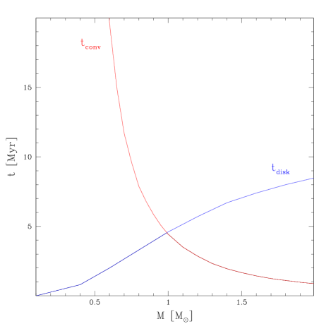
Figure 2: Proto-stellar disk lifetime ($t_{disk}$; from Li & Xiao, 2016, blue line) and duration of the fully convective phase ($t_{conv}$; from Tognelli, Prada Moroni, & Degl’Innocenti, 2011, red line) as a function of the stellar mass.

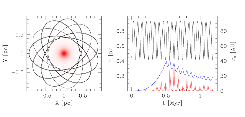
Figure 3: Orbit of a sample star in simulation R14.4lm6rh1 (left panel). The location of the gas is marked by the red area. The corresponding evolution of the distance from the cluster centre (black), the proto-stellar disk truncation radius (blue) and the accretion rate (red) are shown in the right panel.

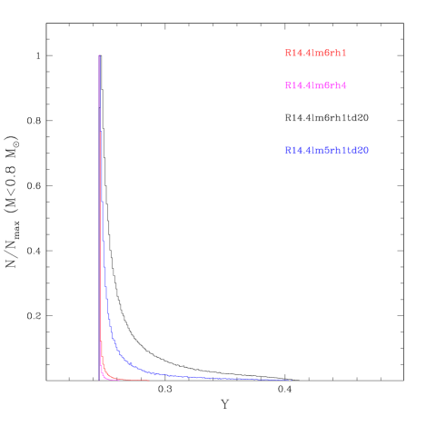
Figure 4: Distribution of He mass fration in the simulations run within the accretion onto proto-stellar disks scenario. All histograms are normalized to the peak value.

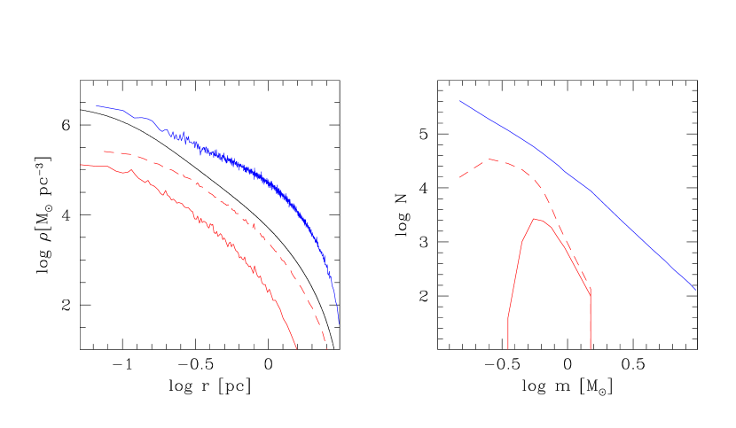
Figure 5: Initial density (left panel) profiles and mass functions (right panel) of FP (blue lines) and SP (red lines) in the R14.4lm6rh1 (solid lines) and R14.4lm6rh1td20 (dashed lines) simulations. The gas density profile is overplotted in the left panel with a black line.

In the scenario proposed by Bastian et al. (2013), there is only one star formation episode where the FP forms in a mass segregated configuration. After a few Myr massive ($>10~{}M_{\odot}$) stars evolve and release part of their gas in the central region of the cluster. Low-mass stars, still in their pre-Main Sequence phase, cross this region and accrete this gas onto their proto-stellar disks, mixing it with their own gas. To account for the abundance variation of elements involved in the nuclear burning (e.g. He), it is necessary that the accreted material is brought from the surface to the stellar core, an occurrence possible only until the star is entirely convective (D’Antona et al., 2014).

To calculate the amount of gas accreted by low-mass stars, I performed an analytical modeling of the disk structure.

The initial population is distributed in the phase-space according to a multi-mass models of Gunn & Griffin (1979) with $W_{0}=25$. For this purpose, the simulated stellar population has been grouped in 29 mass bins, where stars with masses $M>10~{}M_{\odot}$ are in the last 11 bins.

The gas cloud density profile has been derived as

$$\rho_{g}=\sum_{i=19}^{29}\mu_{i}n_{i}m_{i}$$

where $m_{i}$ is the mass, $\mu_{i}$ is the fraction of released gas (from Kruijssen, 2009), $n_{i}$ is the number density of the stars in the i-th mass bin.

The orbits of less-massive ($M<10~{}M_{\odot}$) stars within the cluster potential are followed using a 4th-order Runge-Kutta integrator for the time their proto-stellar disks are able to accrete gas ($t_{end}$). This timescale has been calculated as the minimum between the disk lifetime ($t_{disk}$) and the time during which the star is entirely convective ($t_{conv}$). I adopted the disk lifetimes calculated by Li & Xiao (2016) (LX16) as a function of the stellar mass. According to these authors, the proto-stellar disk survives longer in massive stars than in low-mass ones, ranging from 0.8 Myr in a 0.4 $M_{\odot}$ star to 8.5 Myr in a 2 $M_{\odot}$ star. Note that these models are built assuming the disk formed by gas in stable rotation. This condition can be altered in the case of a strong accretion of gas at low angular momentum, so that the stability of the disk is not guaranteed (Wijnen et al., 2016). The time a star maintain a fully convective structure has been taken from the pre-Main Sequence evolutionary tracks of Tognelli, Prada Moroni, & Degl’Innocenti (2011) with a metal content Z=0.001. The dependence of $t_{disk}$ and $t_{conv}$ as a function of the stellar mass is shown in Fig. 2. It can be seen that the time during which the proto-star is able to accrete gas and use it as a fuel in its core is a peaked function of mass with a maximum duration of $\sim 5$ Myr at the mass of $M\sim 1~{}M_{\odot}$. As hypothesized by Bastian et al. (2013), the gas accretion can prolong the disk lifetime. To account for this effect, the orbit integration is interrupted when the integration time exceeds the instantaneous value of $t_{end}(M(t))$. Moreover, to account for the uncertain modeling of disk lifetimes, additional simulations were performed assuming an increased lifetime $t_{disk}=20~{}Myr$ regardless of the stellar mass.

The gas crossing the disk during this time interval (i.e. the maximum amount of gas that can be accreted by the star) is given by

$$\Delta M=\int_{0}^{t_{end}}\pi~{}r_{d}^{2}~{}\rho_{g}~{}v~{}\cos{\alpha}~{}dt$$

where $v$ is the modulus of the star velocity, $r_{d}$ is the proto-stellar disk radius and $\alpha$ is the angle between the star position and velocity vectors. All the above quantities are time-dependent and are calculated along the star orbit.

In case of isolated stars, the models of Nakamoto & Nakagawa (1994) and Li & Xiao (2016) indicate that the disk radius grows with time until a gravitational instability occurs or X-ray photoevaporation destroy the outer regions of the disk (Owen, Clarke, & Ercolano, 2012), at distances as large as 50 AU. This is confirmed by the existence of extremely extended disks (up to 1000 AU; Lada et al., 2000) around young stars in the Trapezium cluster. However, within a dense cluster the main truncation mechanism for disks is the close passage of nearby stars. To account for this effect I applied a Monte Carlo scheme to implement the technique developed by de Juan Ovelar et al. (2012) locally along the orbit followed by the star inside the cluster. At each point along the orbit, $10^{5}$ synthetic particles have been extracted with the local mass function and the corresponding velocity distribution. An impact parameter

$$b=b_{max}\sqrt{\eta}$$

has been extracted, with $\eta$ being a random number uniformly distributed between 0 and 1, $n$ is the local number density and

$$b_{max}=\left(\frac{48}{\pi~{}n}\right)^{1/3}$$

The truncation radius implied by the encounter with a star colliding with the extracted mass $m^{\prime}$, impact parameter $b$, and a relative velocity with modulus $w$, is given by

$$r_{tr}^{\prime}(w,m^{\prime},b)=\frac{G(m+m^{\prime})}{w^{2}(1+\sqrt{m^{\prime}/m})}\left(\sqrt{1+\frac{b~{}w^{2}}{G(m+m^{\prime})}}-1\right)$$

The total number of collisions occurring with impact parameter $b<b_{max}$ before the time $t$ is instead given by

$$N_{coll}=0.3\pi b_{max}^{2}n\langle w\rangle t$$

where $\langle w\rangle$ is averaged over the $10^{5}$ synthetic particles and the coefficient 0.3 is a corrective factor accounting for the mild effect of encounters occurring with inclination angles $>45^{\circ}$ (de Juan Ovelar et al., 2012). The individual values of $r_{tr}^{\prime}$ are sorted and a relation between the ranking index and $r_{tr}^{\prime}$ is derived. The instantaneous truncation radius ($t_{tr,t}$), set by the most likely closest collision, is then defined by interpolating through the above relation at the index $i^{\prime}=10^{5}/N_{coll}$.

The disk radius at the given time and in a given point along the star orbit is finally given by

$$r_{d}=min\left[31\left(\frac{t}{5\cdot 10^{5}yr}\right)^{3}pc,~{}r_{tr,t}\right]$$

To compute the actual enhancement provided by the accretion process, the total He mass fraction has been calculated assuming a cosmological He abundance for the FP (Y=0.245; Planck Collaboration et al., 2016) and the extreme He abundance predicted by de Mink et al. (2009)

$$Y=\frac{0.245~{}M_{0}+0.44~{}\Delta M}{M_{0}+\Delta M}$$

where $M_{0}$ is the original stellar mass before accretion.

The evolution of the accretion rate of a sample star in the R14.4lm6rh1td20 simulation during its first Myr is shown in Fig. 3. This star, after moving for 20 Myr within the inner pc, reaches a final mass of 0.14 $M_{\odot}$ and a He mass fraction $Y=0.3$. It can be noted that the maximum accretion occurs during pericenters, where the gas density and the star speed are high. The accretion rate is however modulated according to the size of the proto-stellar disk which increases at the beginning of the disk evolution, reaches a maximum and then progressively declines as a result of the cumulative effect of close collisions. Consequently, most of the accretion occurs at early epochs, while after a few Myr the disk is almost unable to accrete gas anymore.

The distributions of He mass fractions among low-mass ($M<0.8~{}M_{\odot}$; i.e. those expected to survive after a Hubble time) for the four considered initial conditions are shown in Fig. 4. It is immediately apparent that in all simulations, the distribution is unimodal with a peak at the cosmological value ($Y=0.245$) and a tail toward high Y mass fractions. In the absence of any apparent bimodality, I conventionally assigned stars with $Y>0.3$ to the SP. In all simulations adopting the disk lifetimes predicted by the LX16 model the fraction of SP stars is negligible ($M_{S}/M_{tot}<1\%$). A slightly larger fraction of SP ($\sim 8\%$) is instead predicted by simulations adopting an extended disk lifetime, although it is far below the observed value in the majority of GCs ($>60\%$; Carretta et al., 2009; Milone et al., 2017). Note also that, for a fixed half-mass radius, the larger the initial cluster mass the larger is the abundance of SP, in agreement with what observed among GCs (Carretta et al., 2010). This is due to the increasing density and mean velocity in massive clusters, leading to large accretion rates. For the same reason, the simulation starting with a large half-mass radius (R14.4lm6rh4) has a smaller fraction of SP stars with respect to the simulation with a small half-mass radius and the same mass (R14.4lm6rh1).

The initial density profiles of gas, FP and SP for the simulation R14.4lm6rh1 and R14.4lm6rh1td20 are shown in the left panel of Fig. 5. It can be seen that, in both simulations, the SP naturally forms more concentrated than FP, and follows a density profile similar to that of the polluted gas. However, only a small fraction of the gas is used to form the SP. Another peculiarity of this scenario is related to the resulting mass functions of the two populations (see the right panel of Fig. 5). Indeed, while the FP forms with the standard Kroupa (2001) IMF, the SP is able to accrete efficiently gas only in a restricted range of mass, thus following a mass function peaked at $log~{}(M/M_{\odot}\sim-0.3$, with a steep slope $\alpha\sim-5$ at masses $-0.3<log(M/M_{\odot})<0.2$ and deprived of stars outside the mass range $-0.5<log(M/M_{\odot})<0.2$. Qualitatively, the same evidence is apparent in simulations where the disk lifetime has been increased to 20 Myr at all masses. In this case, low-mass stars have more time to accrete gas, so that the SP is more abundant and the mass function peak is shifted at a lower mass.

4 Results

4.1 Cooling flow scenario

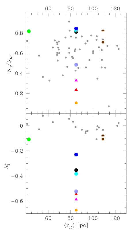
Figure 6: Fraction of SP (top panel) and $A_{2}^{+}$ parameter (bottom panel) measured in the last snapshot of all the simulations run within the cooling flow scenario. Grey points represents the observational fractions for the Galactic GCs (from Milone et al., 2017; Dalessandro et al., 2019). The colour code is described in the last column of Table 1. Circles and triangles represent simulations with and without primordial mass segregation. The symbol size is proportional to the initial Roche-lobe filling factor $r_{h}/r_{J}$.

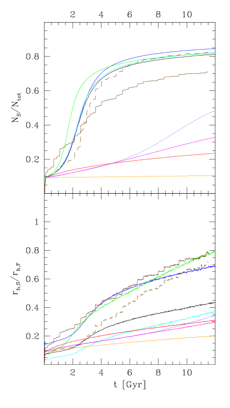
Figure 7: Evolution of the SP number fraction (top panel) and SP/FP half-mass radii (bottom panel) for all the simulations run within the cooling flow scenario. The colour code is described in the last column of Table 1.

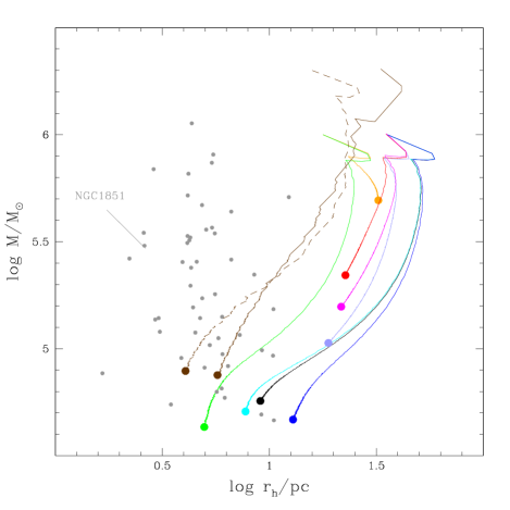
Figure 8: Evolution of all the simulations run within the cooling flow scenario in the $M-r_{h}$ plane. The large dots mark the endpoints of the simulations. Grey points represents the Galactic GCs with $70<\langle r_{J5}\rangle/pc<100$. The location of NGC1851 is also indicated. The colour code is described in the last column of Table 1.

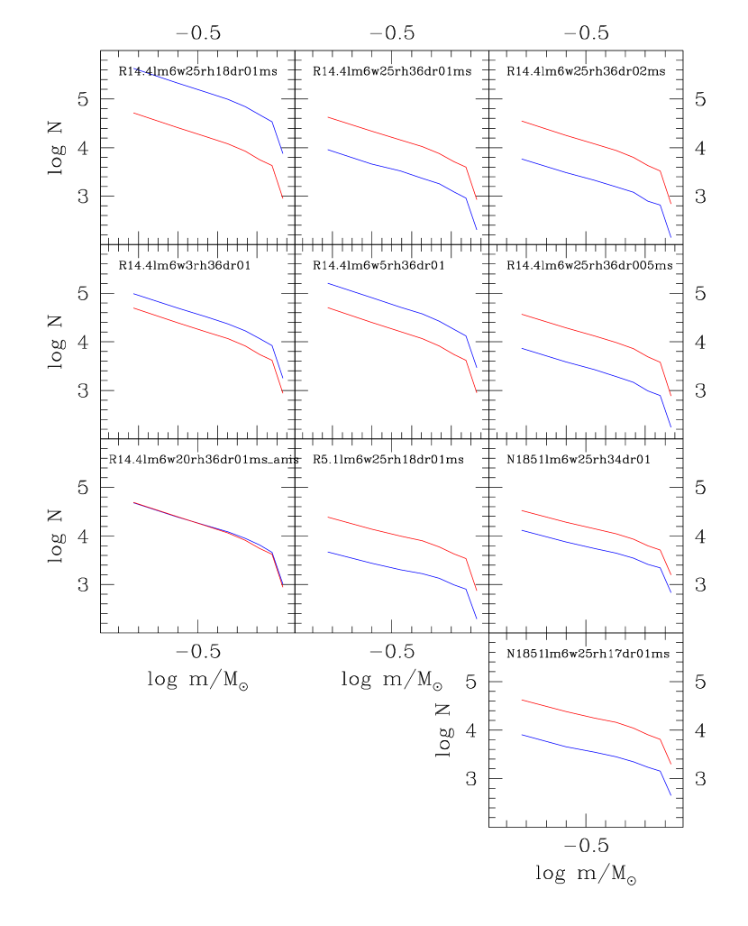
Figure 9: Mass function of FP (blue line) and SP (red line) measured in the last snapshot of all the simulations run within the cooling flow scenario.

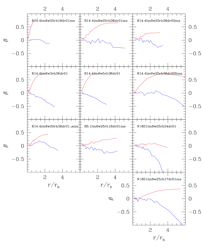
Figure 10: Anisotropy parameter of FP (blue lines) and SP (red lines) as a function of the distance from the cluster centre measured in the last snapshot of the simulations run according to the cooling flow scenario. Distances are normalized to the final global half-mass radius.

In the top panel of Fig. 6 the fractions of SP stars in the last snapshot of the 10 simulations run within the cooling flow scenario are plotted against the orbit-averaged Jacobi radius (i.e. indicating the strength of the tidal field they are subject to) and compared with the fractions measured in Galactic GCs by Milone et al. (2017). Among simulations moving on a circular orbit, it can be noted that both simulations starting without primordial mass segregation (R14.4lm6w5rh36dr01 and R14.4lm6w3rh36dr01) predict a fraction of SP stars $N_{S}/N_{tot}<0.4$, significantly smaller than that observed in real GCs. Between them, the simulation with a shallower density profile (R14.4lm6w3rh36dr01) loses slightly more FP stars than the one with the steeper profile (R14.4lm6w5rh36dr01). This is expected since in the former simulation a larger fraction of FP stars is located at large distances from the cluster centre with respect to the latter simulation which is more concentrated and therefore more resistant to evaporation (see also Vesperini, 1997). Among simulations with primordial mass segregation, the fraction of SP stars presents a strong dependence on the Roche-lobe filling factor, with the most tidally-filling simulations ($r_{h}/r_{J}\geq 0.15$) able to reach the large observational values. Both the above evidences are expected as a result of the increasing amount of mass loss (mainly FP stars) experienced by simulations starting with primordial mass segregation and with a large filling factor. Indeed, the potential energy lost in the cluster centre is given by $\Delta\Phi=\sum G\Delta m_{i}/r_{i}$, where $\Delta m_{i}$ is the mass lost by the i-th star because of stellar evolution and $r_{i}$ is the distance of the star from the cluster centre. In mass segregated simulations massive stars (subject to a large amount of mass loss) are preferentially located at small distances, so that the loss of potential energy is larger than in non-segregated simulations. These simulations strongly expand to maintain the virial equilibrium pushing FP stars, preferentially located in the peripheral cluster region, outside the Jacobi radius. In the same way, the larger is the initial Roche-lobe filling factor the larger is the fraction of stars exceeding the Jacobi radius during this early expansion. Instead, SP stars segregated in the cluster centre remain at the bottom of the potential well and are more efficiently retained until the end of the simulation. The subsequent evolution has only a minor effect in the global fraction of SP stars. This process is depicted in the top panel of Fig. 7, where the evolution of the number ratio of FP and SP stars of the 10 simulations are compared.

To investigate the degree of mass segregation of SP stars, the parameter $A_{2}^{+}$ (Dalessandro et al., 2019) has been calculated. For this purpose, the 3D positions of particles with masses $m>0.7~{}M_{\odot}$ have been projected on the plane of the sky assuming an isotropic spherical symmetry. The cumulative distributions of FP/SP stars located within $2~{}r_{h}$ from the cluster centre, have been computed and normalized to their respective total numbers. The $A_{2}^{+}$ parameter is then calculated as the difference of the integrals of the two distributions. In the bottom panels of Fig. 6 the values of $A_{2}^{+}$ computed on the last snapshot of the 10 simulations are plotted against $\langle r_{J5}\rangle$ and compared with those estimated by Dalessandro et al. (2019) for 18 Galactic GCs. Note that, while real GCs show values of $-0.11<A_{2}^{+}<0.08$ with a weak decreasing trend with $\langle r_{J5}\rangle$, at the end of all the simulations moving on circular orbits at a distance $R_{g}=14.4~{}kpc$ the SP is much more segregated in the centre ($A_{2}^{+}<-0.2$). The evolution of the ratio of the SP and FP half-mass radii in the various simulations is shown in the bottom panel of Fig. 7. It is apparent that SP expands at most by a factor of 4 at the end of these simulations. This is a consequence of the long relaxation time of these simulations which reduces the efficiency of the dynamical mixing between the two populations. The half-mass relaxation time (Spitzer, 1987) is indeed $t_{rh}>20~{}Gyr$ at the beginning of all these simulations and remains longer than 3 Gyr during their entire evolution. Note that the dynamical mixing efficiency of the two populations depends on the tidal truncation and not on the initial half-mass radius. Indeed, the same discrepancy is present in the underfilling simulations R14.4lm6w25rh18dr01ms which, in spite of its relatively short initial half-mass relaxation time, quickly expand without loosing a significant amount of mass, thus increasing their half-mass relaxation time during their evolution. A better agreement is instead found with simulation R5.1lm5w25rh18dr01ms starting with a small half-mass radius while being tidally-filling. In this last case, the tidal cut keeps the simulation compact with a relaxation time which is short enough to allow the two populations to efficiently mix. It is also interesting to note that, comparing simulations R14.4lm6w25rh36dr005ms, R14.4lm6w25rh36dr01ms and R14.4lm6w25rh36dr02ms, the initial concentration of the SP has only a minor effect on both the SP fraction and on its radial segregation. In fact the SP/FP ratio mainly depends on the efficiency of evaporation of the FP, while the SP is almost unaffected by mass loss. Moreover the SP, when initially more concentrated, expands faster and partially compensates for the initial condition.

In Fig. 8 the evolution of the 10 simulations in the mass vs. half-mass radius plane is shown. For comparison, the location of Galactic GCs with $70<\langle r_{J5}\rangle/pc<100$ is shown (see Sect. 3). The evolution of all simulations follows in this plane a characteristic path: an initial expansion (due to the stellar evolution-driven mass loss) followed by a temporary contraction of the half-mass (due to the formation of the SP in the centre), and a subsequent phase where both mass and half-mass radius decrease. The length of the path depends mainly on the initial Roche-lobe filling factor $r_{h}/r_{J}$, with tidally-filling clusters evolving toward a less massive and more concentrated structure than underfilling ones. All the simulation starting with a Roche-lobe filling factor $r_{h}/r_{J}>0.15$ loose $>90\%$ of their initial mass and reach after 12 Gyr masses significantly smaller ($0.5<\Delta log(M/M_{\odot})<0.8$) than the mean present-day mass of GCs ($\langle log(M/M_{\odot})\rangle\sim 5.4$).

Summarizing, by analysing the set of simulations moving within the simplified point-mass galactic potential following circular orbits, it seems that only tidally-filling simulations with a significant degree of primordial mass segregation can reproduce the large fraction of SP found in Galactic GCs. This configuration however lead to the emergence of SP with a degree of radial segregation which is incompatible with observations, unless strong tidal fields are considered. This can be a big problem for the cooling flow scenario considering that $\langle r_{J5}\rangle$ varies by more than an order of magnitude among the Galactic GC system.

A solution is provided by the simulations moving in the axisymmetric potential of Johnston, Spergel, & Hernquist (1995) and following the eccentric orbit of NGC1851 (N1851lm6.3w25rh34dr01 and N1851lm6.3w25rh17dr01ms). These simulations, although starting in underfilling conditions, suffer strong mass loss during the peri-Galactic passages and the disk crossing. During the simulation, the half-mass radius is set at a reduced size with respect to a simulation moving on a circular orbit, being characterized by a shorter half-mass relaxation time. Consequently, both the fraction of SP stars and the $A_{2}^{+}$ turn out to be consistent with the observational values, in spite of the apparently large value of $\langle r_{J5}\rangle$. Moreover, in these simulations primordial mass segregation is not a necessary condition: also the simulation without primordial mass segregation (N1851lm6w25rh34dr01) can indeed reproduce the fraction of SP.

In Fig. 9 the mass functions of FP and SP measured in the last snapshot of all simulations are shown. The mass functions of both populations are very similar, with slopes comprised in the range $-1.2<\alpha<-0.6$ and a maximum difference of $\Delta\alpha<0.15$ (i.e. with the FP with a slightly flatter MF than the SP), in agreement with what found by Vesperini et al. (2018). As expected, because of the preferential loss of low-mass stars (Baumgardt & Makino, 2003), simulations loosing a large fraction of their initial mass are those with the flattest mass function.

The anisotropy parameter $\beta\equiv 1-\sigma_{t}^{2}/\sigma_{r}^{2}$ (where $\sigma_{r}$ and $\sigma_{t}$ are the dispersions of the radial and tangential component of the velocity) is plotted as a function of the distance from the cluster centre in Fig.10 for all the 10 simulations. Apart from small differences, in all the simulations the FP shows an anisotropy profile declining at large radii toward the regime of tangential anisotropy ($\beta<0$), while the SP shows the opposite trend. This result is almost independent on the initial degree of anisotropy of the FP (see simulations R14.4lm6w25rh36dr01ms and R14.4lm6w20rh36dr01ms_anis). This occurs because of the strong effect of tidal forces on the FP which favour the evaporation of stars on radial orbits. On the other hand, the SP is less affected by tides and preserves its original radial anisotropy. The results presented here agree with those of Hénault-Brunet et al. (2015). The simulations of Tiongco, Vesperini, & Varri (2019) also predict a similar behaviour in the early stages of evolution while after many relaxation times they predict isotropic profiles for both FP and SP. Given the extremely long relaxation time of the simulations presented here, the predictions of these works can be considered in agreement.

4.2 Accretion onto proto-stellar disks scenario

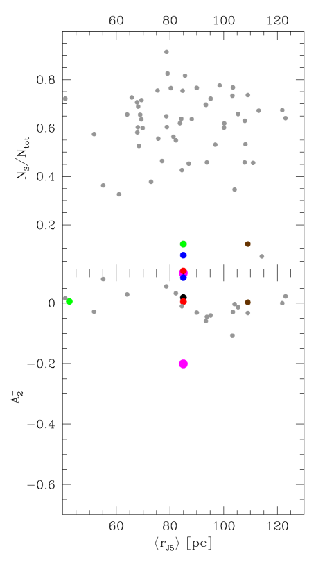
Figure 11: Same as Fig. 6 but for the simulations run according to the accretion onto proto-stellar disks scenario.

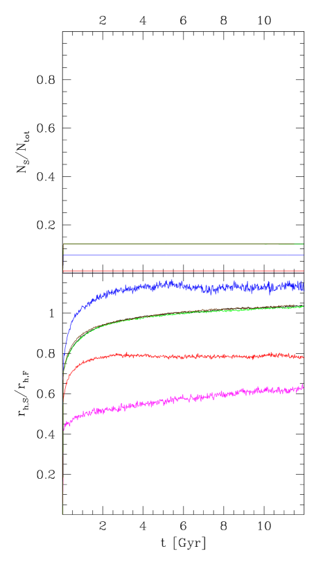
Figure 12: Same as Fig. 7 but for the simulations run according to the accretion onto proto-stellar disks scenario.

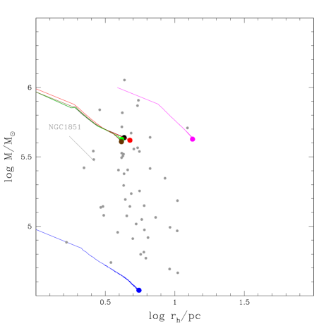
Figure 13: Same as Fig. 8 but for the simulations run according to the accretion onto proto-stellar disks scenario.

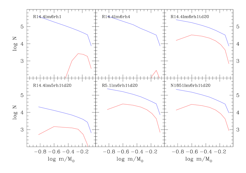
Figure 14: Same as Fig. 9 but for the simulations run according to the accretion onto proto-stellar disks scenario.

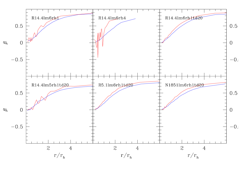
Figure 15: Same as Fig. 10 but for the simulations run according to the accretion onto proto-stellar disks scenario.

In Fig. 11 the fraction of SP and the $A_{2}^{+}$ value measured un the last snapshot of the 6 simulations run according to the accretion onto proto-stellar disks scenario. All the 6 simulations lead to very small SP fraction ($N_{S}/N_{tot}<0.13$). This is not surprising given the extremely small initial fraction of SG (see Sect. 3.2). In this scenario all the simulations start in underfilling conditions both to form a significant SP and to reproduce the present-day half-mass radius of GCs. Moreover, the SP is only mildly more concentrated than FP at the beginning of these simulations. So, both FP and SP are free to expand and interact during the subsequent evolution without a preferential loss of FP stars, thus leaving the fraction of SP stars almost unchanged. This is apparent in the top panel of Fig. 12 where the evolution of the SP fraction is shown for all the 6 simulations.

Regarding the radial distribution of SP, all the simulations with an increased disk lifetime have SP completely mixed with FP. As shown in the bottom panel of Fig. 12, in compact and underfilling conditions, two-body relaxation is efficient in mixing the two populations at early epochs, while the dynamical evolution at later times ($t>2~{}Gyr$; after the stellar evolution-driven expansion) only marginally affects the radial segregation of SP. In this respect, simulations with extended disk lifetimes host a SP containing a larger fraction of low-mass stars (see Fig. 5) and a more extended radial distribution with respect to simulations with the disk lifetimes predicted by the LX16 model.

In Fig. 13 the evolution of the 6 considered simulations in the mass vs. half-mass radius plane is shown. Most simulations show the same behaviour with an expansion (driven by stellar evolution) and a modest mass loss ($\Delta log(M/M_{\odot})\sim 0.3$; almost entirely addressed to stellar evolution mass loss). In this case, simulations with an initial mass of $M=10^{6}~{}M_{\odot}$ and half-mass radius $r_{h}=1~{}pc$ well reproduce after 12 Gyr the average present-day mass and half-mass radius of Galactic GCs.

Note also that in this scenario the simulations run in a simplified potential (R14.4lm6rh1td20 and R5.1lm6rh1td20) and that run in the axisymmetric potential (N1851lm6rh1td20) produce very similar results. Indeed, in all these simulations, the entire cluster is always contained in a small volume well inside the Jacobi radius.

In Fig. 14 the mass functions of the two populations at the end of the 6 simulations are compared. The strong mass function difference observed at the beginning of the simulation (Sect. 3.2) remains apparent also after 12 Gyr in all the considered simulations. This is not surprising given the relatively small amount of mass lost by both populations. In particular, while the FP has a mass function consistent with a power-law, the mass function of the SP is significantly depleted of low-mass ($M<0.3~{}M_{\odot}$) stars.

The anisotropy profiles measured in the last snapshot of the 6 simulations are shown in Fig. 15. In all simulations, both populations show a radially anisotropic profile. This is a consequence of the many close encounters occurring in the dense cluster centres which eject stars of both populations on radial orbits at large distances (Lynden-Bell & Wood, 1968; Spitzer & Shull, 1975). The behaviour of the anisotropy profiles shown in Fig. 15 differs from that predicted by the simulations of Hénault-Brunet et al. (2015). In the simulations of these authors indeed the FP is isotropic at the end of the evolution, similarly to what happens in the cooling flow scenario, while the SP is radially anisotropic at large radii. The difference between the two works likely resides in the different initial structure of the simulations. The simulations of Hénault-Brunet et al. (2015) are indeed $\sim$1000 time less dense than the simulations run here, so that the number of close collisions occurring in their centres is much lower.

5 Summary

I presented the results of a large set of Monte Carlo simulations of star clusters run adopting the initial conditions predicted by the two main scenarios proposed so far for the formation of multiple populations. These simulations, containing $1.5\div 3\cdot 10^{6}$ particles, are among the largest simulations ever run and allow for the first time to reach final masses similar or only a factor $\sim 5$ smaller than those of real GCs.

For the accretion onto proto-stellar disks scenario, the accretion rate of individual disks has been modeled for the first time, accounting for the evolution of the size of the proto-stellar disk. Because of the short disk-lifetimes, only a negligible fraction of polluted material can be accreted onto the proto-stellar disks of low-mass stars. Even adopting a mass-independent disk lifetime of 20 Myr, the SP do not exceed 10% of the whole stellar content. Moreover, the continuous distribution of orbital energies leads to a continuous distribution of the time spent by stars within the polluted gas cloud, thus avoiding the formation of discrete populations. Because of the small disk radii at low masses and the quick disappearance of the convective proto-stellar core, the IMF of SP is depleted of low- ($M<0.3~{}M_{\odot}$) and high-mass ($M>1.5~{}M_{\odot}$) stars. The subsequent dynamical evolution does not significantly change any of the above initial differences. Indeed, the initial density required to constitute a significant amount of polluted gas implies an initially concentrated structure ($r_{h}(0)=1~{}pc$), so that the cluster remains extremely resistant to tidal effects and retains a large fraction of stars of both populations. The final fraction of SP turns out to be therefore inconsistent with those observed today in Galactic GCs (Milone et al., 2017). Several works foresaw the difficulty of this scenario in producing discrete populations (see e.g. Renzini, 2008) and in maintaining an efficient convective core for a significant amount of time (D’Antona et al., 2014), although this is the first time these problems are quantified. These issues adds to the already known problems of this scenario in reproducing the Li abundance of SP (D’Antona et al., 2014) and the stability of disks in a strong-accretion regime (Wijnen et al., 2016).

The simulations run under the cooling flow scenario, given the large number of involved free parameters, are instead able to reproduce at the end of their evolution the present-day general properties of FP/SP (in terms of their relative fraction and radial segregation) reaching a global structure comparable (i.e. a similar half-mass radius and a slightly lower mass) to those of Galactic GCs. The imperative conditions to provide a good agreement are however that the cluster i) form in a tidally-filling configuration ($r_{h}/r_{J}>0.15$; although this condition depends on the initial SP/FP mass ratio) and ii) maintains a compact structure during its evolution. The first condition ensures a large fraction of SP stars, while the second allows the spatial mixing of the two populations. Indeed, the larger is the filling-factor, the more efficient is the loss of FP determining the final proportion of SP/FP. On the other hand, the smaller is the cluster size the shorter is the relaxation time, thus increasing the efficiency of two-body relaxation. The lack of a decreasing trend between the relative fraction of SP with the Galactocentric distance implies that the above conditions must be fulfilled at all Galactocentric distances. This can represent a big problem for the cooling flow scenario. Indeed, in a logarithmic potential (like the one of the Milky Way halo; Johnston, Spergel, & Hernquist, 1995), the Jacobi radius grows as $r_{J}\propto R_{g}^{2/3}$. So, to keep the filling-factor fixed, the initial half-mass radius of the cluster should grow accordingly. It is therefore impossible to satisfy both the above conditions across the large range of Galactocentric distances ($0.5<R_{g}/kpc<125$ Harris, 1996, 2010 edition) covered by Galactic GCs. In particular, at large Galactocentric distances GCs the Galactic tidal field is so weak that the cluster spend all its life with a large half-mass radius constituting a non-collisional environments where the SP would maintain a strong radial segregation (reaching $r_{h,S}/r_{h,F}\sim 0.2$), much stronger than what observed among Galactic GCs. This problem would be further amplified if smaller fractions of SP/FP would be assumed (as proposed by Cabrera-Ziri et al., 2015). Moreover, it is difficult to explain how star formation can ignite in the extremely low-density environment required by this scenario in GCs in the outer Galactic halo. A solution to this problem can be linked to the orbits distribution of Galactic GCs. The two simulations run in the axisymmetric potential of Johnston, Spergel, & Hernquist (1995) and following the eccentric orbit of NGC1851 both conclude their evolutions with a SP with a reasonable fraction and radial distribution in spite of their large present-day Galactocentric distance. In these cases, disk- and bulge-shocks contribute to trigger the mass loss of FP and to keep the cluster in a compact configuration, even if the cluster starts in an underfilling condition. Of course, the shape of the Galactic potential and the orbital eccentricity cannot erase the weakening of the tidal strength at large Gactocentric distances. However, it is known that GCs orbits become radially anisotropic in the outer halo (Vasiliev, 2019), and this can contribute to maintain a significant tidal truncation also for GCs at large Galactocentric distances. Unfortunately, only a single eccentric orbit has been considered here, so that it is not clear if such an effect can solve the above problem for the GCs along the entire range of Galactocentric distances. Further surveys of simulations, tailored to reproduce the observed SP/FP population ratios and following the actual orbit of a significant number of GCs are necessary to clarify this issue.

It is interesting to note that the two considered scenarios foresee opposite predictions for the mass functions and the anisotropy profiles of FP and SP. The determination of these quantities can therefore be good tools to distinguish between these two scenarios. In particular, while in the cooling flow scenario no significant differences are expected in the mass function of FP and SP, in the accretion onto proto-stellar disks scenario the SP should show a significant depletion of low-mass ($M<0.3~{}M_{\odot}$) masses. Unfortunately, the only available study of this kind (Milone et al., 2012) is focused on the very central region of the cluster where the effect of mass segregation produces strong modifications to the global mass function. Similarly, while in the cooling flow scenario the FP is characterized by a significantly smaller degree of radial anisotropy than the SP, in the accretion onto proto-stellar disks scenario the two populations are expected to share the same anisotropic profile. However, observational studies provide conflicting results, with some clusters hosting stellar populations with similar anisotropy profiles and others with significant differences (Cordoni et al., 2020).

In the present paper, I do not compare the predicted behaviour of other kinematic parameters of FP and SP like e.g. binary and remnant fraction. While these quantities contain important information, their present-day appearance strongly depend on their uncertain initial conditions. Future work will be addressed to investigate the evolution of these quantities spanning a wide range in their initial conditions.

Data availability

The data underlying this article will be shared on reasonable request to the corresponding author.

Table 1: Initial and final properties of the performed simulations.

	Initial								Final
name	$R_{g}$	Mass	$W_{0}$	$M_{F}$	$r_{h}$	$M_{S}/M_{tot}$	$r_{h,S}/r_{h,F}$	$r_{h}/r_{J}$	M	$r_{h}$	$N_{S}/N_{tot}$	$A_{2}^{+}$	colour	$t_{disk}$
		segregation												/Note
	kpc			$10^{5}~{}M_{\odot}$	pc				$10^{5}~{}M_{\odot}$	pc				Myr
Cooling flow scenario
R14.4lm6w5rh36dr01	14.4	no	5	10	36	0.091	0.10	0.200	2.21	22.68	0.235	-0.546	red
R14.4lm6w3rh36dr01	14.4	no	3	10	36	0.091	0.10	0.200	1.57	21.66	0.329	-0.585	magenta
R14.4lm6w25rh36dr01ms	14.4	yes	25	10	36	0.091	0.10	0.200	0.57	9.08	0.812	-0.336	black
R14.4lm6w25rh18dr01ms	14.4	yes	25	10	18	0.091	0.10	0.100	4.94	32.30	0.105	-0.093	orange
R5.1lm6w25rh18dr01ms	5.1	yes	25	10	18	0.091	0.10	0.200	0.43	4.97	0.818	-0.672	green
R14.4lm6w25rh36dr005ms	14.4	yes	25	10	36	0.091	0.05	0.200	0.51	7.74	0.825	-0.365	cyan
R14.4lm6w25rh36dr02ms	14.4	yes	25	10	36	0.091	0.20	0.200	0.47	12.91	0.845	-0.222	blue
R14.4lm6w20rh36dr01ms_anis	14.4	yes	20	10	36	0.091	0.10	0.200	1.06	18.88	0.485	-0.525	indigo	anis FP/isot SP
N1851lm6.3w5rh34dr01	NGC1851-like	no	5	20	34	0.091	0.10	0.094	0.75	5.73	0.710	-0.111	brown
N1851lm6.3w25rh17dr01ms	NGC1851-like	yes	25	20	17	0.091	0.10	0.047	0.79	4.06	0.824	-0.072	brown-dashed
Accretion onto proto-stellar disks scenario
R14.4lm6rh1	14.4	yes	25	10	1	0.012	0.57	0.005	4.17	4.75	0.010	0.001	red	LX16
R14.4lm6rh4	14.4	yes	25	10	4	0.002	0.43	0.022	4.25	13.42	0.001	-0.188	magenta	LX16
R14.4lm6rh1td20	14.4	yes	25	10	1	0.082	0.70	0.005	4.35	4.32	0.121	0.019	black	20
R14.4lm5rh1td20	14.4	yes	25	1	1	0.052	0.73	0.005	0.35	5.52	0.075	0.114	blue	20
R5.1lm6rh1td20	5.1	yes	25	10	1	0.082	0.70	0.005	4.23	4.15	0.121	0.014	green	20
N1851lm6rh1td20	NGC1851-like	yes	25	10	1	0.082	0.70	0.003	4.07	4.13	0.121	0.012	brown	20

References

- Aguilar, Hut, & Ostriker (1988) Aguilar L., Hut P., Ostriker J. P., 1988, ApJ, 335, 720
- Allen, Moreno, & Pichardo (2006) Allen C., Moreno E., Pichardo B., 2006, ApJ, 652, 1150
- Bastian et al. (2013) Bastian N., Lamers H. J. G. L. M., de Mink S. E., Longmore S. N., Goodwin S. P., Gieles M., 2013, MNRAS, 436, 2398
- Bastian, Cabrera-Ziri, & Salaris (2015) Bastian N., Cabrera-Ziri I., Salaris M., 2015, MNRAS, 449, 3333
- Bastian & Lardo (2018) Bastian N., Lardo C., 2018, ARA&A, 56, 83
- Baumgardt & Makino (2003) Baumgardt H., Makino J., 2003, MNRAS, 340, 227
- Baumgardt et al. (2019) Baumgardt H., Hilker M., Sollima A., Bellini A., 2019, MNRAS, 482, 5138
- Bellini et al. (2015) Bellini A., Vesperini E., Piotto G., Milone A. P., Hong J., Anderson J., van der Marel R. P., et al., 2015, ApJL, 810, L13
- Bellini et al. (2018) Bellini A., Libralato M., Bedin L. R., Milone A. P., van der Marel R. P., Anderson J., Apai D., et al., 2018, ApJ, 853, 86
- Cabrera-Ziri et al. (2015) Cabrera-Ziri I., Bastian N., Longmore S. N., Brogan C., Hollyhead K., Larsen S. S., Whitmore B., et al., 2015, MNRAS, 448, 2224
- Calura et al. (2019) Calura F., D’Ercole A., Vesperini E., Vanzella E., Sollima A., 2019, MNRAS, 489, 3269
- Carretta et al. (2009) Carretta E., Bragaglia A., Gratton R. G., Lucatello S., Catanzaro G., Leone F., Bellazzini M., et al., 2009, A&A, 505, 117
- Carretta et al. (2010) Carretta E., Bragaglia A., Gratton R. G., Recio-Blanco A., Lucatello S., D’Orazi V., Cassisi S., 2010, A&A, 516, A55
- Cassisi & Salaris (2014) Cassisi S., Salaris M., 2014, A&A, 563, A10
- Chatterjee et al. (2010) Chatterjee S., Fregeau J. M., Umbreit S., Rasio F. A., 2010, ApJ, 719, 915
- Cordero et al. (2017) Cordero M. J., Hénault-Brunet V., Pilachowski C. A., Balbinot E., Johnson C. I., Varri A. L., 2017, MNRAS, 465, 3515
- Cordoni et al. (2020) Cordoni G., Milone A. P., Mastrobuono-Battisti A., Marino A. F., Lagioia E. P., Tailo M., Baumgardt H., et al., 2020, ApJ, 889, 18
- Dalessandro et al. (2019) Dalessandro E., Cadelano M., Vesperini E., Martocchia S., Ferraro F. R., Lanzoni B., Bastian N., et al., 2019, ApJL, 884, L24
- D’Antona et al. (2014) D’Antona F., Ventura P., Decressin T., Vesperini E., D’Ercole A., 2014, MNRAS, 443, 3302
- Decressin et al. (2007) Decressin T., Meynet G., Charbonnel C., Prantzos N., Ekström S., 2007, A&A, 464, 1029
- Decressin, Baumgardt, & Kroupa (2008) Decressin T., Baumgardt H., Kroupa P., 2008, A&A, 492, 101
- de Juan Ovelar et al. (2012) de Juan Ovelar M., Kruijssen J. M. D., Bressert E., Testi L., Bastian N., Cánovas H., 2012, A&A, 546, L1
- de Mink et al. (2009) de Mink S. E., Pols O. R., Langer N., Izzard R. G., 2009, A&A, 507, L1
- D’Ercole et al. (2008) D’Ercole A., Vesperini E., D’Antona F., McMillan S. L. W., Recchi S., 2008, MNRAS, 391, 825
- D’Ercole et al. (2010) D’Ercole A., D’Antona F., Ventura P., Vesperini E., McMillan S. L. W., 2010, MNRAS, 407, 854
- D’Ercole et al. (2012) D’Ercole A., D’Antona F., Carini R., Vesperini E., Ventura P., 2012, MNRAS, 423, 1521
- Duquennoy & Mayor (1991) Duquennoy A., Mayor M., 1991, A&A, 500, 337
- Fregeau & Rasio (2007) Fregeau J. M., Rasio F. A., 2007, ApJ, 658, 1047
- Gieles et al. (2018) Gieles M., Charbonnel C., Krause M. G. H., Hénault-Brunet V., Agertz O., Lamers H. J. G. L. M., Bastian N., et al., 2018, MNRAS, 478, 2461
- Giersz (1998) Giersz M., 1998, MNRAS, 298, 1239
- Giersz (2001) Giersz M., 2001, MNRAS, 324, 218
- Giersz et al. (2013) Giersz M., Heggie D. C., Hurley J. R., Hypki A., 2013, MNRAS, 431, 2184
- Gratton et al. (2019) Gratton R., Bragaglia A., Carretta E., D’Orazi V., Lucatello S., Sollima A., 2019, A&ARv, 27, 8
- Gunn & Griffin (1979) Gunn J. E., Griffin R. F., 1979, AJ, 84, 752
- Harris (1996) Harris W. E., 1996, AJ, 112, 1487
- Hénault-Brunet et al. (2015) Hénault-Brunet V., Gieles M., Agertz O., Read J. I., 2015, MNRAS, 450, 1164
- Hénon (1971) Hénon M. H., 1971, Ap&SS, 14, 151
- Hong et al. (2015) Hong J., Vesperini E., Sollima A., McMillan S. L. W., D’Antona F., D’Ercole A., 2015, MNRAS, 449, 629
- Hong et al. (2016) Hong J., Vesperini E., Sollima A., McMillan S. L. W., D’Antona F., D’Ercole A., 2016, MNRAS, 457, 4507
- Hut & Bahcall (1983) Hut P., Bahcall J. N., 1983, ApJ, 268, 319
- Johnston, Spergel, & Hernquist (1995) Johnston K. V., Spergel D. N., Hernquist L., 1995, ApJ, 451, 598
- Joshi, Rasio, & Portegies Zwart (2000) Joshi K. J., Rasio F. A., Portegies Zwart S., 2000, ApJ, 540, 969
- Joshi, Nave, & Rasio (2001) Joshi K. J., Nave C. P., Rasio F. A., 2001, ApJ, 550, 691
- Khalaj & Baumgardt (2015) Khalaj P., Baumgardt H., 2015, MNRAS, 452, 924
- King (1966) King I. R., 1966, AJ, 71, 64
- Krause et al. (2013) Krause M., Charbonnel C., Decressin T., Meynet G., Prantzos N., 2013, A&A, 552, A121
- Kremer et al. (2020) Kremer K., Ye C. S., Rui N. Z., Weatherford N. C., Chatterjee S., Fragione G., Rodriguez C. L., et al., 2020, ApJS, 247, 48
- Kroupa (2001) Kroupa P., 2001, MNRAS, 322, 231
- Kruijssen (2009) Kruijssen J. M. D., 2009, A&A, 507, 1409
- Lada et al. (2000) Lada C. J., Muench A. A., Haisch K. E., Lada E. A., Alves J. F., Tollestrup E. V., Willner S. P., 2000, AJ, 120, 3162
- Langer, Hoffman, & Sneden (1993) Langer G. E., Hoffman R., Sneden C., 1993, PASP, 105, 301
- Lardo et al. (2011) Lardo C., Bellazzini M., Pancino E., Carretta E., Bragaglia A., Dalessandro E., 2011, A&A, 525, A114
- Lee & Nelson (1988) Lee H. M., Nelson L. A., 1988, ApJ, 334, 688
- Li & Xiao (2016) Li M., Xiao L., 2016, ApJ, 820, 36
- Lind et al. (2011) Lind K., Charbonnel C., Decressin T., Primas F., Grundahl F., Asplund M., 2011, A&A, 527, A148
- Lynden-Bell & Wood (1968) Lynden-Bell D., Wood R., 1968, MNRAS, 138, 495
- Merritt (1985) Merritt D., 1985, AJ, 90, 1027
- Milone et al. (2012) Milone A. P., Piotto G., Bedin L. R., Cassisi S., Anderson J., Marino A. F., Pietrinferni A., et al., 2012, A&A, 537, A77
- Milone et al. (2017) Milone A. P., Piotto G., Renzini A., Marino A. F., Bedin L. R., Vesperini E., D’Antona F., et al., 2017, MNRAS, 464, 3636
- Morscher et al. (2013) Morscher M., Umbreit S., Farr W. M., Rasio F. A., 2013, ApJL, 763, L15
- Nakamoto & Nakagawa (1994) Nakamoto T., Nakagawa Y., 1994, ApJ, 421, 640
- Osipkov (1979) Osipkov L. P., 1979, PAZh, 5, 77
- Ostriker, Spitzer, & Chevalier (1972) Ostriker J. P., Spitzer L., Chevalier R. A., 1972, ApJL, 176, L51
- Owen, Clarke, & Ercolano (2012) Owen J. E., Clarke C. J., Ercolano B., 2012, MNRAS, 422, 1880
- Pancino et al. (2007) Pancino E., Galfo A., Ferraro F. R., Bellazzini M., 2007, ApJL, 661, L155
- Pietrinferni et al. (2006) Pietrinferni A., Cassisi S., Salaris M., Castelli F., 2006, ApJ, 642, 797
- Piotto (2006) Piotto G., 2006, IAUJD, JD 14, id. 10
- Piotto et al. (2015) Piotto G., Milone A. P., Bedin L. R., Anderson J., King I. R., Marino A. F., Nardiello D., et al., 2015, AJ, 149, 91
- Planck Collaboration et al. (2016) Planck Collaboration, Ade P. A. R., Aghanim N., Arnaud M., Ashdown M., Aumont J., Baccigalupi C., et al., 2016, A&A, 594, A13
- Renzini (2008) Renzini A., 2008, MNRAS, 391, 354
- Sollima, Bellazzini, & Lee (2012) Sollima A., Bellazzini M., Lee J.-W., 2012, ApJ, 755, 156
- Sollima & Mastrobuono Battisti (2014) Sollima A., Mastrobuono Battisti A., 2014, MNRAS, 443, 3513
- Sollima & Ferraro (2019) Sollima A., Ferraro F. R., 2019, MNRAS, 483, 1523
- Spitzer & Shull (1975) Spitzer L., Shull J. M., 1975, ApJ, 201, 773
- Spitzer (1987) Spitzer L., 1987, in "Dynamical Evolution of globular clusters", Princeton University Press, Princeton NJ"
- Tiongco, Vesperini, & Varri (2019) Tiongco M. A., Vesperini E., Varri A. L., 2019, MNRAS, 487, 5535
- Tognelli, Prada Moroni, & Degl’Innocenti (2011) Tognelli E., Prada Moroni P. G., Degl’Innocenti S., 2011, A&A, 533, A109
- Vasiliev (2015) Vasiliev E., 2015, MNRAS, 446, 3150
- Vasiliev (2019) Vasiliev E., 2019, MNRAS, 484, 2832
- Ventura et al. (2013) Ventura P., Di Criscienzo M., Carini R., D’Antona F., 2013, MNRAS, 431, 3642
- Vesperini (1997) Vesperini E., 1997, MNRAS, 287, 915
- Vesperini et al. (2011) Vesperini E., McMillan S. L. W., D’Antona F., D’Ercole A., 2011, MNRAS, 416, 355
- Vesperini et al. (2013) Vesperini E., McMillan S. L. W., D’Antona F., D’Ercole A., 2013, MNRAS, 429, 1913
- Vesperini et al. (2018) Vesperini E., Hong J., Webb J. J., D’Antona F., D’Ercole A., 2018, MNRAS, 476, 2731
- Wijnen et al. (2016) Wijnen T. P. G., Pols O. R., Pelupessy F. I., Portegies Zwart S., 2016, A&A, 594, A30
- Yoshida (1990) Yoshida H., 1990, PhLA, 150, 262