On the interpretation of $\Lambda$ spin polarization measurements

Abstract

The physics interpretation of the recent measurements of the spin polarization of $\Lambda$ hyperons produced in relativistic heavy-ion collisions is discussed. We suggest that the polarization measured in the $\Lambda$ rest frame should be projected along the direction of the total angular momentum that is first transformed to the same frame, and only then averaged over $\Lambda$’s with different momenta in the center-of-mass frame. While this procedure does not affect the current measurements done in a broad transverse-momentum range, it may become important (represent a correction of about 10%) for the most energetic hyperons under study (with transverse momenta reaching 4–5 GeV/c). The proposed treatment is generally more appropriate for relativistic $\Lambda$’s. Throughout the paper, we deliver explicit expressions for various boosts, rotations, and transformations of angular distributions, which may help to compare model predictions with the experimental results.

I Introduction

For a few decades now the phenomenon of spin polarization of the $\Lambda$ hyperons produced in proton-proton and heavy-ion collisions has been an intriguing topic of both experimental and theoretical investigations Bunce et al. (1976); Bourrely et al. (1980); Panagiotou (1990); Becattini et al. (2021). For example, the longitudinal polarization of the ${\bar{\Lambda}}$ hyperons was discussed in 1980s as a possible signal of the quark-gluon plasma formation Jacob and Rafelski (1987). However, the first heavy-ion experiments that measured the $\Lambda$ spin polarization in Dubna Anikina et al. (1984) and at CERN Bartke et al. (1990) reported negative results. More recently, several theoretical predictions of the global spin polarization signal in A+A collisions were given in Refs. Liang and Wang (2005); Betz et al. (2007); Voloshin (2004). These works predicted a rather substantial experimental signal, of the order of 10%, and were not confirmed by the STAR data of 2007 Abelev et al. (2007). The idea of a non-vanishing global polarization reappeared in the context of statistical physics and equilibration of spin degrees of freedom Becattini and Piccinini (2008); Becattini et al. (2008); Becattini et al. (2013a, b); Becattini et al. (2017). The much smaller predictions of this approach Karpenko and Becattini (2017); Li et al. (2017); Xie et al. (2017); Sun and Ko (2017) have been eventually observed by STAR Adamczyk et al. (2017); Adam et al. (2018) and independently by ALICE Acharya et al. (2020). This has triggered a vast theoretical interest that includes several highly debated topics: the importance of the spin-orbit coupling Gao et al. (2008); Chen et al. (2009), global equilibrium with a rigid rotation Becattini and Tinti (2010); Becattini (2012); Becattini and Grossi (2015); Hayata et al. (2015), hydrodynamic Florkowski et al. (2018a, b, 2019a); Li et al. (2021); Hu (2021) and kinetic Gao et al. (2012); Chen et al. (2013); Fang et al. (2016, 2017); Florkowski et al. (2018c); Weickgenannt et al. (2019, 2021); Bhadury et al. (2021a, b); Tinti and Florkowski (2020) models of spin dynamics, anomalous hydrodynamics Son and Surowka (2009); Kharzeev and Son (2011), the Lagrangian formulation of hydrodynamics Montenegro et al. (2017a, b), and hydrodynamic treatment of spin currents in the presence of torsion Gallegos et al. (2021). For recent reviews of the experimental and theoretical situation see, for example, Refs. Huang (2021); Becattini and Lisa (2020); Florkowski et al. (2019b); Speranza and Weickgenannt (2021); Bhadury et al. (2021c).

As the outcome of the spin polarization experiments, one commonly cites the magnitude of the polarization along a specific direction in the center-of-mass frame (COM). Most preferably, the results refer to the direction that is orthogonal either to the reaction plane (RP, in non-central heavy-ion collisions) Becattini et al. (2021) or to the production plane (in proton-proton collisions) Bunce et al. (1976); Panagiotou (1990). In the case of heavy ions, the direction transverse to the reaction plane agrees with the direction of the total angular momentum of the system ${\bm{L}}$ (with the orientation of ${\bm{L}}$ opposite to the $y$ axis, see Fig. 1).

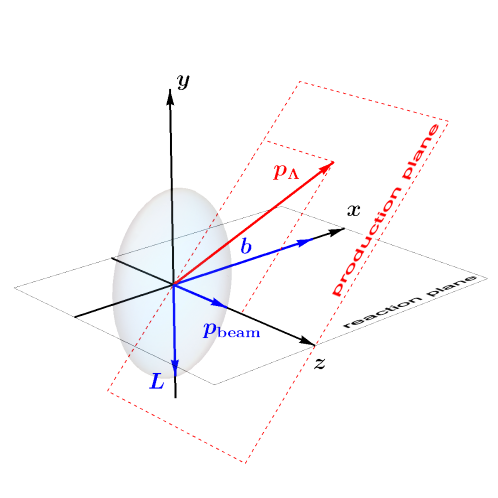
Figure 1: The center-of-mass (COM) frame for non-central heavy-ion collisions. In this case both the reaction and production planes can be defined.

To determine the magnitude of the polarization in different directions, however, one first studies distributions of various three-momentum components of protons emitted in the weak decay $\Lambda\to p+\pi^{-}$, which are measured in the $\Lambda$ rest frame. As the COM frame and the $\Lambda$ rest frame are connected by the Lorentz transformation depending on the three-momentum of $\Lambda$, the spatial directions in these two frames are linked by a non-trivial relation. Consequently, relating the results obtained in the $\Lambda$ rest frame to the global angular momentum direction of the system requires that an appropriate Lorentz transformation is done before one describes such results in terms of the COM variables.

The STAR measurements Adamczyk et al. (2017); Adam et al. (2018); Acharya et al. (2020) indicate that the proton distributions in the $\Lambda$ rest frame are not isotropic and, consequently, unambiguously lead to the conclusion about the non-zero $\Lambda$ spin polarization. In our opinion, however, the interpretation of those results in the context of specific correlations between the spin direction of $\Lambda$’s and various directions in COM (in particular, the direction of the total orbital angular momentum ${\bm{L}}$) requires further clarifications because of at least two reasons. First, typically only one component of the polarization vector is measured — the $y$-component in the $\Lambda$ rest frame. Second, the $y$ direction in the $\Lambda$ rest frame is different from the $y$ direction in COM.  Consequently, a complete understanding of the relation between the $\Lambda$ spin direction and the direction of the total orbital angular momentum in COM calls for a more detailed study of the effect connected with the boost to the $\Lambda$ rest frame.

This is especially important if one interprets the result of the $\Lambda$ polarization measurements as an analog of the Einstein-de Haas or the Barnett effect Einstein and de Haas (1915); Barnett (1935). In this case, we suggest first to measure the projection of the spin polarization along the orbital angular momentum direction that is “seen” by a $\Lambda$ in its rest frame, and only then to make averaging over $\Lambda$’s with different momenta in COM. Such a method guarantees that the same physical direction is used for all $\Lambda$’s. We do not expect that such a procedure may change any qualitative conclusions about the global spin polarization but, in our opinion, it is more appropriate to establish the right magnitude of the polarization and its energy dependence.

We note that an alternative method for measurements of the global polarization of $\Lambda$’s has been proposed in Ref. Siddique et al. (2019), where one demonstrates that the measurements can use quantities defined in the laboratory frame (instead of the quantities defined in the $\Lambda$’s rest frame). However, this work does not discuss the effects connected with a change of the orbital angular momentum direction due to the boosts, which is the main topic of the present analysis.

In this work, we give several explicit expressions for boosts, rotations, and transformations of angular distributions that can be useful whenever model predictions are compared with the experimental results. In particular, we give an expression for the form of the angular momentum in the $\Lambda$ rest frame that can be used to consistently project the polarization of $\Lambda$’s measured in their rest frames.

The paper is organized as follows: In the next section, we define the center-of-mass (COM) frame for heavy-ion and proton-proton collisions. In Sec. III we introduce the canonical boost from COM to the $\Lambda$ rest frame and introduce the transformation of the total angular three-momentum from COM to the $\Lambda$ rest frame. Yet another $\Lambda$ rest frame, where the $\Lambda$ polarization is aligned with the $z$ axis, is introduced in Sec. IV. The weak decay law for the process $\Lambda\to p+\pi^{-}$ is introduced in Sec. V. Finally, in Sec. VI we discuss our main point regarding the projection of the measured polarization on the total angular momentum in COM. We summarize and conclude in Sec. VIII. Several useful properties of the canonical boost and transformations of the angular distributions of protons are discussed in the two appendices.

Conventions and notation: Throughout the paper we use natural units with $\hbar=c=1$ and the metric tensor with the signature $(+---)$. Three- and four-vectors are defined by their components, however, for three-vectors we often use the bold font, for example, $p^{\mu}=(E,p^{1},p^{2},p^{3})=(E,{\bm{p}})$, where $E=\sqrt{m^{2}+p^{2}}$ denotes the particle energy. For the length of a three-vector we use the regular font, $p=|{\bm{p}}|$. Scalar products of three-vectors are denoted by a dot, $a^{\mu}b_{\mu}=a^{0}b^{0}-{\bm{a}}\cdot{\bm{b}}$. The unit three-vectors are denoted by a hat so that ${\bm{p}}=p\,\hat{{\bm{p}}}$.

II center-of-mass (COM) frame

In the analyzes of spin polarization of relativistic particles, it is important to define precisely the reference frames where the specific physical quantities are defined and measured. In this work, we define altogether three different reference frames that are linked by Lorentz boosts and rotations: the center-of-mass frame of the total system, COM, and two rest frames of $\Lambda$’s with a given momentum in COM. The last two frames differ by rotation.

We assume that the main reference frame corresponds to the center-of-mass frame of the colliding system. In the case of non-central heavy-ion collisions, the axes of the COM frame are defined by the beam axis ($\hat{\bm{z}}$), the impact vector ($\hat{\bm{x}}$), and the direction that is perpendicular to the reaction plane ($\hat{\bm{y}}$) spanned by $\hat{\bm{x}}$ and $\hat{\bm{z}}$, see Fig. 1.  We note that the orientation of the three-vector describing the orbital angular momentum ${\bm{L}}$ is opposite to the $y$ axis.

In the case of proton-proton collisions, the $z$ axis corresponds to the direction of the initial protons, the $y$ axis is defined to be perpendicular to the plane determined by $\hat{\bm{z}}$ and the momentum of the emitted $\Lambda$ hyperon ${\bm{p}}_{\Lambda}$, i.e., to the production plane, while $\hat{\bm{x}}$ is perpendicular to both $\hat{\bm{y}}$ and $\hat{\bm{z}}$, see Fig. 2. The Cartesian coordinate system $x,y,z$ is taken in the two cases to be right-handed. We note that in the case of proton-proton collisions one may also use a rotated frame where the $z$ axis coincides with the direction of ${\bm{p}}_{\Lambda}$. In Fig. 2 the axes of this frame are denoted by $x_{r}$, $y_{r}$, and $z_{r}$.

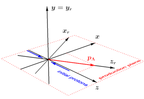
Figure 2: The center-of-mass (COM) frame for $p$+$p$ collisions.

III The $\Lambda$ rest frame $S^{\prime}({\bm{p}}_{\Lambda})$

In the following, we define two frames where the $\Lambda$ hyperon with the momentum ${\bm{p}}_{\Lambda}$ in COM frame is at rest. The first one is defined by the canonical boost from the COM frame. The second one differs from the first by an additional rotation that aligns the polarization vector with the $z$-axis.

III.1 The canonical boost

We define the rest frame $S^{\prime}({\bm{p}}_{\Lambda})$ of $\Lambda$’s with the COM frame three-momentum ${\bm{p}}_{\Lambda}=(p^{1}_{\Lambda},p^{2}_{\Lambda},p^{3}_{\Lambda})$ by the canonical boost Jackson (1998); Leader (2011)

$${\cal L}^{\mu}_{\,\,\,\nu}\left(-{{\bm{v}}}_{\Lambda}\right)=\left[\begin{array}[]{cccc}\frac{E_{\Lambda}}{m_{\Lambda}}&-\frac{p^{1}_{\small\Lambda}}{m_{\Lambda}}&-\frac{p^{2}_{\Lambda}}{m_{\Lambda}}&-\frac{p^{3}_{\Lambda}}{m_{\Lambda}}\\ -\frac{p^{1}_{\Lambda}}{m_{\Lambda}}&1+\alpha p^{1}_{\Lambda}p^{1}_{\Lambda}&\alpha p^{1}_{\Lambda}p^{2}_{\Lambda}&\alpha p^{1}_{\Lambda}p^{3}_{\Lambda}\\ -\frac{p^{2}_{\Lambda}}{m_{\Lambda}}&\alpha p^{2}_{\Lambda}p^{1}_{\Lambda}&1+\alpha p^{2}_{\Lambda}p^{2}_{\Lambda}&\alpha p^{2}_{\Lambda}p^{3}_{\Lambda}\\ -\frac{p^{3}_{\Lambda}}{m_{\Lambda}}&\alpha p^{3}_{\Lambda}p^{1}_{\Lambda}&\alpha p^{3}_{\Lambda}p^{2}_{\Lambda}&1+\alpha p^{3}_{\Lambda}p^{3}_{\Lambda}\end{array}\right].$$ (5)

Here $E_{\Lambda}$ and ${\bm{v}}_{\Lambda}={\bm{p}}_{\Lambda}/E_{\Lambda}$ are the energy and three-velocity of $\Lambda$ in COM, respectively, while $m_{\Lambda}$ is the $\Lambda$ mass and $\alpha\equiv 1/\left(m_{\Lambda}\left(E_{\Lambda}+m_{\Lambda}\right)\right)$. We stress that the frame $S^{\prime}({\bm{p}}_{\Lambda})$ depends on ${\bm{p}}_{\Lambda}$ – in practice one should select an ensemble of events that include $\Lambda$’s with the COM three-momentum in a small bin placed around a given value of ${\bm{p}}_{\Lambda}$. The components of the four-vectors in $S^{\prime}({\bm{p}}_{\Lambda})$ and COM are related by the transformation

$$p^{\prime\mu}={\cal L}_{\,\,\,\nu}^{\mu}\left(-{{\bm{v}}}_{\Lambda}\right)p^{\nu}.$$ (6)

In particular, by construction we obtain $p^{\prime\mu}_{\Lambda}=(m_{\Lambda},0,0,0)$.

It is well known Leader (2011) that the canonical boost can be represented as a superposition of three transformations: the rotation ${\cal R}_{\Lambda}$ that brings the three-vector ${\bm{p}}_{\Lambda}$ to the form $(0,0,p_{\Lambda})$, the boost ${\cal L}_{3}$ along the third axis with the velocity $-v_{\Lambda}$, and the inverse rotation ${\cal R}_{\Lambda}^{-1}$, namely

$${\cal L}={\cal R}_{\Lambda}^{-1}(\phi_{\Lambda},\theta_{\Lambda}){\cal L}_{3}(-v_{\Lambda}){\cal R}_{\Lambda}(\phi_{\Lambda},\theta_{\Lambda}).$$ (7)

The rotation ${\cal R}_{\Lambda}$ can be written as the product of two rotations. If we use the parametrization ${\bm{p}}_{\Lambda}=p_{\Lambda}\,(\sin\theta_{\Lambda}\,\cos\phi_{\Lambda},\sin\theta_{\Lambda}\,\sin\phi_{\Lambda},\cos\theta_{\Lambda})$ in COM, then ${\cal R}_{\Lambda}={\cal R}_{2}(\theta_{\Lambda}){\cal R}_{3}(\phi_{\Lambda})$, where

$${\cal R}_{3}\left(\phi_{\Lambda}\right)=\left[\begin{array}[]{cccc}1&0&0&0\\ 0&\cos\phi_{\Lambda}&\sin\phi_{\Lambda}&0\\ 0&-\sin\phi_{\Lambda}&\cos\phi_{\Lambda}&0\\ 0&0&0&1\end{array}\right]$$ (12)

and

$${\cal R}_{2}\left(\theta_{\Lambda}\right)=\left[\begin{array}[]{cccc}1&0&0&0\\ 0&\cos\theta_{\Lambda}&0&-\sin\theta_{\Lambda}\\ 0&0&1&0\\ 0&\sin\theta_{\Lambda}&0&\cos\theta_{\Lambda}\end{array}\right].$$ (17)

The boost ${\cal L}_{3}(-v_{\Lambda})$ is defined by the expression

$${\cal L}_{3}(-v_{\Lambda})=\left[\begin{array}[]{cccc}\gamma_{\Lambda}&0&0&-\gamma_{\Lambda}v_{\Lambda}\\ 0&1&0&0\\ 0&0&1&0\\ -\gamma_{\Lambda}v_{\Lambda}&0&0&\gamma_{\Lambda}\end{array}\right],$$ (22)

where $\gamma_{\Lambda}=E_{\Lambda}/m_{\Lambda}$ is the Lorentz factor. Further useful properties of the canonical boost are discussed in Appendix A.

III.2 Transformation of the system’s angular momentum

The crucial role in the discussion and interpretation of the spin-polarization measurements is played by the total angular momentum of the system described by the tensor $J^{\mu\nu}$. It can be decomposed into the orbital and spin parts, $J^{\mu\nu}=L^{\mu\nu}+S^{\mu\nu}$. In non-central heavy-ion collisions, a substantial non-zero orbital part $L^{\mu\nu}$ is generated at the initial stage Becattini et al. (2008). One expects that during the system’s evolution some part of $L^{\mu\nu}$ is transferred to the spin part $S^{\mu\nu}$, of course, with the total angular momentum $J^{\mu\nu}$ being conserved. The generation of a non-zero spin part $S^{\mu\nu}$ may be reflected just by the measured spin polarization of the produced particles. We note that the spin part may be also generated at the very early stages of the collision but one expects anyway that the values of $S^{\mu\nu}$ are negligible compared to $L^{\mu\nu}$.

If one works in the COM frame, only the spatial components of $L^{\mu\nu}$ are different from zero.  They determine the orbital angular momentum of the system through the relation

$$L^{k}=-\frac{1}{2}\epsilon^{kij}L^{ij}.$$ (23)

With the standard orientation of the axes in COM, one expects that the direction of the vector ${\bm{L}}$ is opposite to the $y$ axis, see Fig. 1. The components of ${\bm{L}}$ transform like the components of the magnetic field since they represent spatial components of an antisymmetric tensor $L^{\mu\nu}$. Hence, in the frame $S^{\prime}({\bm{p}}_{\Lambda})$ they are given by the formula Jackson (1998)

$${\bm{L}}^{\prime}=\gamma_{\Lambda}{\bm{L}}-\frac{\gamma^{2}_{\Lambda}}{\gamma_{\Lambda}+1}\,{\bm{v}}_{\Lambda}({\bm{v}}_{\Lambda}\cdot{\bm{L}}).$$ (24)

From Eq. (24) we find the ratio of the lenghts of the vectors ${\bm{L}}^{\prime}$ and ${\bm{L}}$, namely

$$\frac{L^{\prime}}{L}=\gamma_{\Lambda}\left(1-({\bm{v}}_{\Lambda}\cdot\hat{\bm{L}})^{2}\right)^{1/2}.$$ (25)

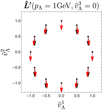
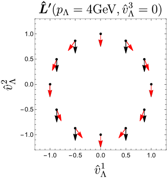
Figure 3: Direction of the total angular momentum of the system transformed from COM to the $S^{\prime}({\bm{p}}_{\Lambda})$ frame (red arrows) for $\Lambda$ particles at midrapidity ($\hat{v}^{z}=0$) with the momentum $p_{\Lambda}=1~{}\text{GeV}$ (left panel) and $p_{\Lambda}=4~{}\text{GeV}$ (right panel) for various orientations of the velocity in transverse plane. Black arrows denote the same quantity as seen in COM.

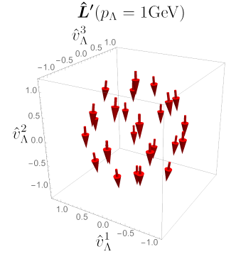
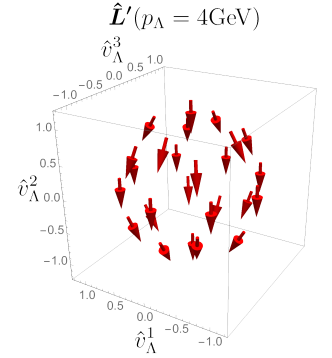
Figure 4: Three-dimensional visualization of the vectors ${\bm{L}}^{\prime}$ defined by Eqs. (24) and (28).

Let us note that for relativistic $\Lambda$’s the directions of ${\bm{L}}$ and ${\bm{L}}^{\prime}$ (measured in their appropriate reference frames) may be significantly different. In general, only for the case ${\bm{v}}_{\Lambda}\cdot{\bm{L}}=0$ they are the same. For non-relativistic systems, the second term on the right-hand side of Eq. (24) represents a relativistic correction of the order $({\bm{v}}_{\Lambda}/c)^{2}$ and can be neglected, however, for relativistic systems the second term may be equally important as the first one. Consequently, comparisons of the measured polarization direction should refer to the direction of ${\bm{L}}^{\prime}$ rather than to the direction of ${\bm{L}}$. For this purpose, we introduce two unit vectors

$$\hat{\bm{L}}=\frac{{\bm{L}}}{L},\quad\hat{\bm{L}}^{\prime}=\frac{{\bm{L}}^{\prime}}{L^{\prime}}.$$ (26)

Taking into account Eq. (25) we may write

$$\hat{\bm{L}}^{\prime}=\left(1-({\bm{v}}_{\Lambda}\cdot\hat{\bm{L}})^{2}\right)^{-1/2}\left(\hat{\bm{L}}-\frac{\gamma_{\Lambda}}{\gamma_{\Lambda}+1}\,{\bm{v}}_{\Lambda}({\bm{v}}_{\Lambda}\cdot\hat{\bm{L}})\right).$$ (27)

This vector is expressed only by the three-momentum of $\Lambda$ and the direction of the angular momentum in COM. We note that with our choice of COM,

$$\hat{\bm{L}}=(0,-1,0)$$ (28)

we obtain

$$\hat{L}^{\prime\,1} = \left(1-(v_{\Lambda}^{2})^{2}\right)^{-1/2}\frac{\gamma_{\Lambda}}{\gamma_{\Lambda}+1}\,v_{\Lambda}^{1}v_{\Lambda}^{2},$$

$$\hat{L}^{\prime\,2} = \left(1-(v_{\Lambda}^{2})^{2}\right)^{-1/2}\left(\frac{\gamma_{\Lambda}}{\gamma_{\Lambda}+1}\,v_{\Lambda}^{2}v_{\Lambda}^{2}-1\right),$$

$$\hat{L}^{\prime\,3} = \left(1-(v_{\Lambda}^{2})^{2}\right)^{-1/2}\frac{\gamma_{\Lambda}}{\gamma_{\Lambda}+1}\,v_{\Lambda}^{3}v_{\Lambda}^{2}.$$ (29)

The visualization of those components for the case $v_{\Lambda}^{3}=0$ is shown in Fig. 4.

For the sake of completeness, let us consider the transformation law for the component $K^{i}=-L^{0i}$ that behaves like an electric-like component of $L^{\mu\nu}$. As we have mentioned above, ${\bm{K}}=0$ in COM. However, after making the canonical boost and using Eq. (28) we obtain

$${\bm{K}}^{\prime}=\gamma_{\Lambda}\left(v_{\Lambda}^{3},0,-v_{\Lambda}^{1}\right)L$$ (30)

or, after normalization,

$$\hat{\bm{K}}^{\prime}=\frac{\left(v_{\Lambda}^{3},0,-v_{\Lambda}^{1}\right)}{\sqrt{(v_{\Lambda}^{1})^{2}+(v_{\Lambda}^{3})^{2}}}.$$ (31)

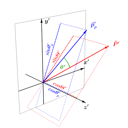
Figure 5: The $\Lambda$ rest frame. The momentum distribution of protons produced in the weak decay $\Lambda\to p+\pi^{-}$ depends on $\cos\theta^{*}$, where $\theta^{*}$ is the angle between the polarization vector ${\bm{P}}^{\prime}$ and the proton momentum direction $\hat{{\bm{p}}}^{\prime}_{p}$.

IV The $\Lambda$ rest frame $S^{*}({\bm{p}}_{\Lambda})$

In the $\Lambda$ rest frame $S^{\prime}({\bm{p}}_{\Lambda})$, the $\Lambda$ polarization is characterized by the polarization three-vector ${\bm{P}}^{\prime}$, see Fig. 5. It can be defined by the magnitude $P^{\prime}$ and the unit vector $\hat{{\bm{P}}}^{\prime}$ that specifies the polarization direction, namely, ${\bm{P}}^{\prime}=P^{\prime}\hat{{\bm{P}}}^{\prime}$. The vector $\hat{{\bm{P}}}^{\prime}$ can be expressed by the two angles $\Phi^{\prime}$ and $\Theta^{\prime}$ with the help of the standard parametrization

$$\hat{{\bm{P}}}^{\prime}=\left(\sin\Theta^{\prime}\cos\Phi^{\prime},\sin\Theta^{\prime}\sin\Phi^{\prime},\cos\Theta^{\prime}\right).$$ (32)

In the following, it will be useful to consider also the frame where only the third component of $\hat{{\bm{P}}}^{\prime}$ is different from zero. This is achieved by the subsequent action of the two rotations

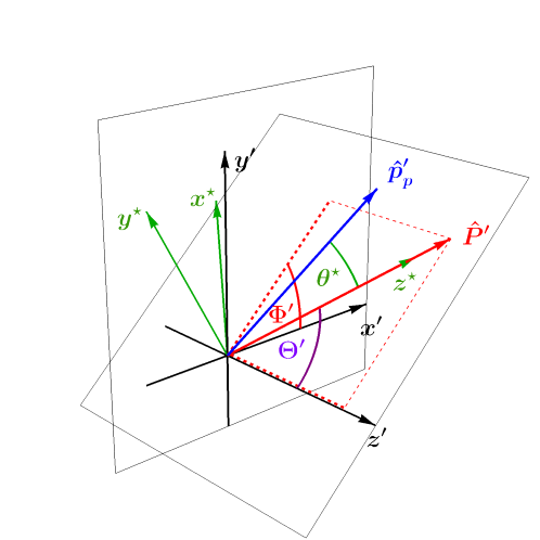
Figure 6: The frame $S^{*}({\bm{p}}_{\Lambda})$ is obtained from the frame $S^{\prime}({\bm{p}}_{\Lambda})$ by a rotation that brings ${\bm{P}}^{\prime}$ along the new $z$-axis.

$${\cal R}_{z^{\prime}}\left(\Phi^{\prime}\right)=\left[\begin{array}[]{ccc}\cos\Phi^{\prime}&\sin\Phi^{\prime}&0\\ -\sin\Phi^{\prime}&\cos\Phi^{\prime}&0\\ 0&0&1\end{array}\right]$$ (36)

and

$${\cal R}_{y^{\prime}}\left(\Theta^{\prime}\right)=\left[\begin{array}[]{ccc}\cos\Theta^{\prime}&0&-\sin\Theta^{\prime}\\ 0&1&0\\ \sin\Theta^{\prime}&0&\cos\Theta^{\prime}\end{array}\right].$$ (40)

The resulting frame will be called $S^{*}({\bm{p}}_{\Lambda})$. It is trivial to see that

$$\hat{{\bm{P}}}^{*}={\cal R}_{y^{\prime}}\left(\Theta^{\prime}\right){\cal R}_{z^{\prime}}\left(\Phi^{\prime}\right)\hat{{\bm{P}}}^{\prime}=(0,0,1).$$ (41)

Let us now consider the three-momentum of the proton emitted in the weak decay of $\Lambda$. Similarly to the case of the polarization vector, we express it as follows ${\bm{p}}^{\prime}_{p}=p_{p}^{\prime}\,\hat{{\bm{p}}}^{\prime}_{p}$ where

$$\hat{{\bm{p}}}^{\prime}_{p}=\left(\sin\theta^{\prime}_{p}\cos\phi^{\prime}_{p},\sin\theta^{\prime}_{p}\sin\phi^{\prime}_{p},\cos\theta^{\prime}_{p}\right).$$ (42)

In the frame $S^{*}({\bm{p}}_{\Lambda})$ we have

$$\hat{p}^{*}_{p,x} = \cos(\Phi^{\prime}-\phi^{\prime}_{p})\sin\theta^{\prime}_{p}\cos\Theta^{\prime}-\cos\theta^{\prime}_{p}\sin\Theta^{\prime}\equiv\sin\theta^{*}\cos\phi^{*},$$

$$\hat{p}^{*}_{p,y} = -\sin(\Phi^{\prime}-\phi^{\prime}_{p})\sin\theta^{\prime}_{p}\equiv\sin\theta^{*}\sin\phi^{*},$$

$$\hat{p}^{*}_{p,z} = \cos(\Phi^{\prime}-\phi^{\prime}_{p})\sin\theta^{\prime}_{p}\sin\Theta^{\prime}+\cos\theta^{\prime}_{p}\cos\Theta^{\prime}\equiv\cos\theta^{*}.$$ (43)

From the last line, we find 

$$\hat{{\bm{P}}}^{\prime}\cdot\hat{{\bm{p}}}^{\prime}_{p}=\hat{{\bm{P}}}^{*}\cdot\hat{{\bm{p}}}^{*}_{p}=\cos\theta^{*}.$$ (44)

The angular distributions of protons emitted in the frames $S^{\prime}({\bm{p}}_{\Lambda})$ and $S^{*}({\bm{p}}_{\Lambda})$ satisfy an obvious constraint

$$\int\frac{dN_{p}}{d\Omega^{\prime}}\,\sin\theta^{\prime}_{p}d\theta^{\prime}_{p}d\phi^{\prime}_{p}=\int\frac{dN_{p}}{d\Omega^{*}}\,\sin\theta^{*}_{p}d\theta^{*}_{p}d\phi^{*}_{p},$$ (45)

where the functions $dN_{p}/d\Omega$ behave like scalar functions of the azimuthal and polar angles. Consequently, if the distribution $dN_{p}/d\Omega^{*}$ is a function of $\cos\theta^{*}$ only, for example,

$$\frac{dN_{p}}{d\Omega^{*}}=F(\cos\theta^{*}),$$ (46)

where $F(x)$ is an arbitrary function of $x$, then

$$\frac{dN_{p}}{d\Omega^{\prime}}=F\left(\cos(\Phi^{\prime}-\phi^{\prime}_{p})\sin\theta^{\prime}_{p}\sin\Theta^{\prime}+\cos\theta^{\prime}_{p}\cos\Theta^{\prime}\right).$$ (47)

At the end of this section let us note that the three-vector ${\bm{P}}^{\prime}$ can be interpreted as a spatial part of the four-vector Itzykson and Zuber (1980)

$$P^{\prime\,\mu}=\left(0,{\bm{P}}^{\prime}\right).$$ (48)

In general, we have

$$-1\leq P^{\prime}\cdot P^{\prime}\leq 0.$$ (49)

The case $P^{\prime}\cdot P^{\prime}=-1$ corresponds to a pure state in which the spin projection is $1/2$ in the direction of $\hat{{\bm{P}}}^{\prime}$. The values larger than $-1$ describe a mixed spin state, and eventually the value $P^{\prime}\cdot P^{\prime}=0$ means that the system is unpolarized.

V The weak decay law

In the frame $S^{*}({\bm{p}}_{\Lambda})$, the $\Lambda$ weak decay $\Lambda\to p+\pi^{-}$ is described by the following law that describes the angular distribution of emitted protons

$$\frac{dN^{\rm pol}_{p}}{d\Omega^{*}}=\frac{1}{4\pi}\left(1+\alpha_{\Lambda}{\bm{P}}^{*}\cdot\hat{{\bm{p}}}_{p}^{*}\right).$$ (50)

Here $\alpha_{\Lambda}=0.732$ is the $\Lambda$ decay constant. Equation (50) implies that in $S^{\prime}({\bm{p}}_{\Lambda})$ the proton angular distribution has the form

$$\frac{dN^{\rm pol}_{p}}{d\Omega^{\prime}}=\frac{1}{4\pi}\left[1+\alpha_{\Lambda}P^{\prime}\left(\cos(\Phi^{\prime}-\phi^{\prime}_{p})\sin\theta^{\prime}_{p}\sin\Theta^{\prime}+\cos\theta^{\prime}_{p}\cos\Theta^{\prime}\right)\right].$$ (51)

The averaged values of the three momentum components in $S^{\prime}({\bm{p}}_{\Lambda})$ can be obtained by straightforward integration:

$$\langle\hat{p}^{\prime}_{p,x}\rangle = \int\left(\frac{dN^{\rm pol}_{p}}{d\Omega^{\prime}}\right)(\sin\theta^{\prime}_{p})^{2}\cos\phi^{\prime}_{p}\,d\theta^{\prime}_{p}\,d\phi^{\prime}_{p}=\frac{1}{3}P^{\prime}\alpha_{\Lambda}\sin\Theta^{\prime}\cos\Phi^{\prime},$$

$$\langle\hat{p}^{\prime}_{p,y}\rangle = \int\left(\frac{dN^{\rm pol}_{p}}{d\Omega^{\prime}}\right)(\sin\theta^{\prime}_{p})^{2}\sin\phi^{\prime}_{p}\,d\theta^{\prime}_{p}\,d\phi^{\prime}_{p}=\frac{1}{3}P^{\prime}\alpha_{\Lambda}\sin\Theta^{\prime}\sin\Phi^{\prime},$$

$$\langle\hat{p}^{\prime}_{p,z}\rangle = \int\left(\frac{dN^{\rm pol}_{p}}{d\Omega^{\prime}}\right)\sin\theta^{\prime}_{p}\cos\theta^{\prime}_{p}\,d\theta^{\prime}_{p}\,d\phi^{\prime}_{p}=\frac{1}{3}P^{\prime}\alpha_{\Lambda}\cos\Theta^{\prime}.$$ (52)

Here we have introduced angular brackets to denote angular averaging of the proton variables in the Lambda rest frame $S^{\prime}({\bm{p}}_{\Lambda})$. The last result indicates that the magnitude and direction of the polarization can be directly obtained from the averaged values of the three momentum components measured in $S^{\prime}({\bm{p}}_{\Lambda})$

$${\bm{P}}^{\prime} = P^{\prime}\left(\sin\Theta^{\prime}\cos\Phi^{\prime},\sin\Theta^{\prime}\sin\Phi^{\prime},\cos\Theta^{\prime}\right)=\frac{3}{\alpha_{\Lambda}}\left(\langle\hat{p}^{\prime}_{p,x}\rangle,\langle\hat{p}^{\prime}_{p,y}\rangle,\langle\hat{p}^{\prime}_{p,z}\rangle\right).$$ (53)

One can also find

$$\langle\cos\phi^{\prime}_{p}\rangle = \int\left(\frac{dN^{\rm pol}_{p}}{d\Omega^{\prime}}\right)\,\sin\theta^{\prime}_{p}\cos\phi^{\prime}_{p}\,d\theta^{\prime}_{p}\,d\phi^{\prime}_{p}=\frac{\pi\alpha_{\Lambda}}{8}P^{\prime}\sin\Theta^{\prime}\cos\Phi^{\prime},$$ (54)

$$\langle\sin\phi^{\prime}_{p}\rangle = \int\left(\frac{dN^{\rm pol}_{p}}{d\Omega^{\prime}}\right)\sin\theta^{\prime}_{p}\sin\phi^{\prime}_{p}\,d\theta^{\prime}_{p}\,d\phi^{\prime}_{p}=\frac{\pi\alpha_{\Lambda}}{8}P^{\prime}\sin\Theta^{\prime}\sin\Phi^{\prime}.$$ (55)

The last expression rewritten in the form

$$P_{H}=\frac{8}{\pi\alpha_{\Lambda}}\langle\sin\phi^{\prime}_{p}\rangle$$ (56)

serves as the main experimental tool used to determine the spin polarization.  The two comments are in order now:

• The quantity $P_{H}$ is the $y$-component of the polarization three-vector measured in the Lambda rest frame, namely, $P_{H}=P^{\prime}\sin\Theta^{\prime}\sin\Phi^{\prime}$. Strictly speaking, it is not the component of the polarization along the total angular momentum vector as the $y$-directions in COM and the Lambda rest frame are different (although the differences for slowly moving Lambdas might be quite small).

• In addition to the measurement of the mean $\langle\sin\phi^{\prime}_{p}\rangle$ it is tempting to measure, using the same experimental techniques, the mean $\langle\cos\phi^{\prime}_{p}\rangle$. Such a measurement would complete the analysis of the three components of the polarization vector in the Lambda rest frame, as the longitudinal component has been already measured. The ratio of such measurements would give us directly the information about the angle $\Phi^{\prime}$.

At this point, it is convenient to discuss the effect of the detector magnetic field on the spin polarization. If the $\Lambda$ hyperons move in a magnetic field, their spins undergo precession with the frequency $\omega^{\prime}=g_{\Lambda}\,(\mu_{N}/\hbar)\,B^{\prime}$. Here $g_{\Lambda}=0.613$ is the magnitude of the Landé $g$-factor for $\Lambda$’s, $\mu_{N}$ is the nuclear magneton, and $B^{\prime}$ is the magnitude of the magnetic field in the Lambda rest frame. If $\Lambda$’s move perpendicularly to the magnetic field, the field in the rest frame equals $B^{\prime}=\gamma_{\Lambda}B=\gamma_{\Lambda}\,x\,T$, where we have expressed the value of the magnetic field in COM in units of Tesla, $B=x\,T$. The mean angle by which the spin direction changes equals $\Delta\Phi_{\rm prec}=\omega^{\prime}\Delta t^{\prime}$, where $\Delta t^{\prime}=2.63\cdot 10^{-10}$ s is the mean Lambda lifetime in its rest frame. This altogether gives $\Delta\Phi_{\rm prec}=0.0077\,x\,\gamma_{\Lambda}$. In our opinion, this value represents the systematic error for the experimental estimates of the angles $\Theta^{\prime}$ and $\Phi^{\prime}$. We note that the present STAR estimate of $\Delta\Phi_{\rm prec}$ is somewhat larger, namely, gives 0.022 for $x=0.5$ and $\gamma_{\Lambda}\sim 2$. Nevertheless, this value is used to argue that the effect of the spin precession on the global polarization measurements is negligible. From the point of our analysis, the effects of spin precession require more detailed studies where the impact of precession on the estimates of the angles $\Theta^{\prime}$ and $\Phi^{\prime}$ can be clarified.

VI Correlation with total angular momentum

VI.1 Improved formula for the projection

We have discussed above how the magnitude and direction of the spin polarization can be determined in the frame where $\Lambda$’s are at rest. More precisely, we have considered the rest frame of $\Lambda$’s with three-momentum ${\bm{p}}_{\Lambda}$, which is obtained by the canonical boost from COM. A natural question at this stage appears, how the direction of the measured polarization is related to the axes of the COM coordinate system.

Equation (53) gives the prescription how to measure three independent components of the $\Lambda$ polarization in its (canonical) rest frame. Assuming that the measurement of the averages $\langle\hat{p}^{\prime}_{p,x}\rangle$, $\langle\hat{p}^{\prime}_{p,y}\rangle$, and $\langle\hat{p}^{\prime}_{p,z}\rangle$ is indeed possible, we may define the projection of the polarization along the direction of the total angular momentum by the expression

$$\hat{\bm{L}}^{\prime}\cdot{\bm{P}}^{\prime}=\left(1-({\bm{v}}_{\Lambda}\cdot\hat{\bm{L}})^{2}\right)^{-1/2}\left(\hat{\bm{L}}\cdot{\bm{P}}^{\prime}-\frac{\gamma_{\Lambda}}{\gamma_{\Lambda}+1}\,{\bm{v}}_{\Lambda}\cdot{\bm{P}}^{\prime}\,\,\,{\bm{v}}_{\Lambda}\cdot\hat{\bm{L}}\right).$$ (57)

The direction represented by a unit vector $\hat{\bm{L}}^{\prime}$ is the direction of the total angular momentum that is “seen” by the spin of the decaying $\Lambda$ that has three-momentum ${\bm{p}}_{\Lambda}$ in COM. By construction $|\hat{\bm{L}}^{\prime}\cdot{\bm{P}}^{\prime}|\leq P^{\prime}\leq 1$.

The measurement of the $\Lambda$ spin polarization is very often interpreted as an analog of the Einstein-de Haas and/or the Barnett effect Einstein and de Haas (1915); Barnett (1935). Except for the fact that these two phenomena describe the behavior of a different physical system, one important difference is that for these two effects there exists always a reference frame where all particles are at rest . In the case of spin polarization of $\Lambda$’s, such a frame does not exist, since the analyzed $\Lambda$’s have usually different momenta in COM.

So far, our discussion has been concentrated on $\Lambda$’s with a given momentum in COM. For a given colliding system, beam energy, and the centrality class, such $\Lambda$’s can be treated as produced in the same physical environment (even if they are “taken” from different events) so it makes sense to obtain $\hat{\bm{L}}\cdot{\bm{P}}^{\prime}$ or $\hat{\bm{L}}^{\prime}\cdot{\bm{P}}^{\prime}$ from the proton distributions in $S^{\prime}({\bm{p}}_{\Lambda})$. The advantage of the expression (57) compared to the estimate of just $\hat{\bm{L}}\cdot{\bm{P}}^{\prime}$ is that the spin polarization of each $\Lambda$, irrespectively of its three-momentum ${\bm{p}}_{\Lambda}$ in COM, is projected on the same physical axis corresponding to ${\bm{L}}$ in COM. Hence, Eq. (57) is in our opinion the proper object that can be used to study the relation between the polarization of all $\Lambda$’s with ${\bm{L}}$. To do so, one has to simply average Eq. (57) over all $\Lambda$’s with different ${\bm{p}}_{\Lambda}$.

VI.2 Numerical estimate of the relativistic effects

To make a numerical estimate of the effects discussed above, we consider the case where ${\bm{P}}^{\prime}=P^{\prime}\hat{\bm{L}}$ and

$$\hat{\bm{L}}^{\prime}\cdot{\bm{P}}^{\prime}=P^{\prime}\left(1-v_{2}^{2}\right)^{-1/2}\left(1-\frac{v_{2}^{2}}{1+\sqrt{1-v^{2}}}\,\right)\equiv P^{\prime}F_{P}({\bm{v}})$$ (58)

where $(v_{1},v_{2},v_{3})$ are the components of the $\Lambda$ velocity in COM and $v=\sqrt{v_{1}^{2}+v_{2}^{2}+v_{3}^{2}}$ (to simplify the notation we skip here the subscript $\Lambda$). We further assume that the velocity distribution of Lambdas is thermal and described by the Fermi-Dirac distribution

$$F_{T}(v)=N\left[\exp\left(\frac{m_{\lambda}}{T_{\rm eff}\sqrt{1-v^{2}}}\right)+1\right]^{-1}.$$ (59)

Here $T_{\rm eff}$ is an effective temperature and $N$ is the normalization constant that is irrelevant for our study. The average value of $\hat{\bm{L}}^{\prime}\cdot{\bm{P}}^{\prime}$ for Lambdas with the momentum in the range between $m$ GeV and $n$ GeV is defined as the ratio

$$\langle\hat{\bm{L}}^{\prime}\cdot{\bm{P}}^{\prime}\rangle_{m-n}=P^{\prime}\,\,\frac{\int_{v_{(m)}}^{v_{(n)}}dv\int d\Omega\,F_{P}({\bm{v}})F_{T}(v)}{\int_{v_{(m)}}^{v_{(n)}}dv\int d\Omega\,F_{T}(v)},$$ (60)

where

$$v_{(n)}=\tanh\left[\sinh^{-1}\left(\frac{n\,\rm GeV}{m_{\Lambda}}\right)\right].$$ (61)

The numerical calculations performed with $T_{\rm eff}$ = 150 MeV give: $\langle\hat{\bm{L}}^{\prime}\cdot{\bm{P}}^{\prime}\rangle_{2-3}=0.97~{}P^{\prime}$, $\langle\hat{\bm{L}}^{\prime}\cdot{\bm{P}}^{\prime}\rangle_{3-4}=0.94~{}P^{\prime}$, $\langle\hat{\bm{L}}^{\prime}\cdot{\bm{P}}^{\prime}\rangle_{4-5}=0.92~{}P^{\prime}$, and $\langle\hat{\bm{L}}^{\prime}\cdot{\bm{P}}^{\prime}\rangle_{5-6}=0.90~{}P^{\prime}$. Consequently, the relativistic effects studied in this work may reach 10% for the most energetic Lambdas studied at STAR. However, in the case of momentum-averaged results in the range $0.5-6\mathrm{GeV}/c$ studied in Ref. Adamczyk et al. (2017) one obtains a negligible correction $\langle\hat{\bm{L}}^{\prime}\cdot\bm{P}^{\prime}\rangle_{0.5-6}=0.997P^{\prime}$.

VI.3 Replacing the reaction plane angle by the experimentally-determined event plane angle

Equation (57) is an algebraic equation involving $\hat{\bm{L}}$, which makes the experimental determination of $\hat{\bm{L}}^{\prime}\cdot{\bm{P}}^{\prime}$ more difficult than the measurement of $\hat{\bm{L}}\cdot{\bm{P}}^{\prime}$ alone. This is due to the fact that in the general case the reaction plane is characterized by the angle ${\Psi_{\rm RP}}$ that is not necessarily equal to zero and the direction of the orbital angular momentum is defined by the vector

$$\hat{\bm{L}}=-\left(\cos\left({\Psi_{\rm RP}}+\pi/2\right),\sin\left({\Psi_{\rm RP}}+\pi/2\right),0\right).$$ (62)

We note that for ${\Psi_{\rm RP}}=0$ this formula is reduced to Eq. (28) that has been used so far.

To measure $\hat{\bm{L}}\cdot{\bm{P}}^{\prime}$ in the case ${\Psi_{\rm RP}}\neq 0$ we first perform averaging over the angles of the emitted protons and get

$$\hat{\bm{L}}\cdot{\bm{P}}^{\prime}=-\frac{8}{\pi\alpha_{\Lambda}}\langle\sin(\phi^{\prime}_{p}-{\Psi_{\rm RP}})\rangle=-\frac{8}{\pi\alpha_{\Lambda}}\int\left(\frac{dN^{\rm pol}_{p}}{d\Omega^{\prime}}\right)\sin\left(\phi^{\prime}_{p}-{\Psi_{\rm RP}}\right)\,d\Omega^{\prime}.$$ (63)

This equation introduces an explicit dependence of our results on the reaction plane angle ${\Psi_{\rm RP}}$ which is not directly measured. To overcome this difficulty, the STAR experiment measures the azimuthal angle of the event plane, ${\Psi_{\rm EP}^{(1)}}$, determined by the directed flow. Consequently, one considers the observable

$$\langle\sin(\phi^{\prime}_{p}-{\Psi_{\rm EP}^{(1)}})\rangle_{\rm ev.}=\langle\sin(\phi^{\prime}_{p}-{\Psi_{\rm RP}}-({\Psi_{\rm EP}^{(1)}}-{\Psi_{\rm RP}}))\rangle_{\rm ev.}$$

$$=\langle\sin(\phi^{\prime}_{p}-{\Psi_{\rm RP}})\rangle_{\rm ev.}\langle\cos{\Delta\Psi}\rangle_{\rm ev.}\equiv\langle\sin(\phi^{\prime}_{p}-{\Psi_{\rm RP}})\rangle_{\rm ev.}R^{(1)}_{\rm EP},$$ (64)

where we introduced ${\Delta\Psi}\equiv{\Psi_{\rm EP}^{(1)}}-{\Psi_{\rm RP}}$. In Eq. (64) one assumes that $\phi^{\prime}_{p}$ and ${\Psi_{\rm EP}^{(1)}}$ are correlated only with the reaction plane angle ${\Psi_{\rm RP}}$ and uses the property $\langle\sin{\Delta\Psi}\rangle_{\rm ev.}=0$. The notation $\langle...\rangle_{\rm ev.}$ means that one makes first averaging over different protons in one event and then makes averaging over a sample of events. The last equation in (64) defines the reaction plane resolution factor $R^{(1)}_{\rm EP}$. Using Eq. (64) we find the formula

$$\langle\hat{\bm{L}}\cdot{\bm{P}}^{\prime}\rangle_{\rm ev.}=-\frac{8}{\pi\alpha_{\Lambda}}\langle\sin(\phi^{\prime}_{p}-{\Psi_{\rm RP}})\rangle_{\rm ev.}=-\frac{8}{\pi\alpha_{\Lambda}}\frac{\langle\sin(\phi^{\prime}_{p}-{\Psi_{\rm EP}^{(1)}})\rangle_{\rm ev.}}{R^{(1)}_{\rm EP}},$$ (65)

which is the basis of the experimental approach (for example, see Eq. (19) in Ref. Becattini and Lisa (2020)).

The method used for the measurement of $\hat{\bm{L}}\cdot{\bm{P}}^{\prime}$ suggests a treatment of Eq. (57). Since the expected modifications are at the level of 10% we can make an expansion of the right-hand side of Eq. (57) in powers of $v_{\Lambda}/c$. Up to quadratic terms we obtain

$$\hat{\bm{L}}^{\prime}\cdot{\bm{P}}^{\prime}=\hat{\bm{L}}\cdot{\bm{P}}^{\prime}-\frac{\gamma_{\Lambda}}{\gamma_{\Lambda}+1}\,{\bm{v}}_{\Lambda}\cdot{\bm{P}}^{\prime}\,\,\,{\bm{v}}_{\Lambda}\cdot\hat{\bm{L}}+\frac{1}{2}({\bm{v}}_{\Lambda}\cdot\hat{\bm{L}})^{2}\hat{\bm{L}}\cdot{\bm{P}}^{\prime}.$$ (66)

Consequently, our task is reduced to the determination of the two additional averages: $\langle{\bm{v}}_{\Lambda}\cdot{\bm{P}}^{\prime}\,\,\,{\bm{v}}_{\Lambda}\cdot\hat{\bm{L}}\rangle_{\rm ev.}$ and $\langle({\bm{v}}_{\Lambda}\cdot\hat{\bm{L}})^{2}\hat{\bm{L}}\cdot{\bm{P}}^{\prime}\rangle_{\rm ev.}$.

For the $\Lambda$ hyperons produced at midrapidity (i.e., for $\theta_{\Lambda}=\pi/2$) we may use the property

$$\langle{\bm{v}}_{\Lambda}\cdot{\bm{P}}^{\prime}\,\,\,{\bm{v}}_{\Lambda}\cdot\hat{\bm{L}}\rangle_{\rm ev.}=\frac{8}{\pi\alpha_{\Lambda}}\langle\cos(\phi_{\Lambda}-\phi^{\prime}_{p})\sin(\phi_{\Lambda}-{\Psi_{\rm RP}})\rangle_{\rm ev.}.$$ (67)

To replace the dependence on ${\Psi_{\rm RP}}$ by the dependence on ${\Psi_{\rm EP}^{(1)}}$, we use the equation

$$\langle\cos(\phi_{\Lambda}-\phi^{\prime}_{p})\sin(\phi_{\Lambda}-{\Psi_{\rm RP}})\rangle_{\rm ev.}=\frac{\langle\cos(\phi_{\Lambda}-\phi^{\prime}_{p})\sin(\phi_{\Lambda}-{\Psi_{\rm EP}^{(1)}})\rangle_{\rm ev.}}{\langle\cos(\phi_{\Lambda}-\phi^{\prime}_{p})\cos{\Delta\Psi}\rangle_{\rm ev.}}.$$ (68)

where we used the assumptions that $\langle\cos(\phi_{\Lambda}-\phi^{\prime}_{p})\sin{\Delta\Psi}\rangle_{\rm ev.}=0$. The denominator in the last equation can be treated as another resolution parameter.

In the case of the term $\langle({\bm{v}}_{\Lambda}\cdot\hat{\bm{L}})^{2}\hat{\bm{L}}\cdot{\bm{P}}^{\prime}\rangle_{\rm ev.}$ we use the following property

$$\langle({\bm{v}}_{\Lambda}\cdot\hat{\bm{L}})^{2}\hat{\bm{L}}\cdot{\bm{P}}^{\prime}\rangle_{\rm ev.}=-\frac{8}{\pi\alpha_{\Lambda}}\langle\sin^{2}(\phi_{\Lambda}-{\Psi_{\rm RP}})\sin(\phi^{\prime}_{p}-{\Psi_{\rm RP}})\rangle_{\rm ev.}.$$ (69)

Following the same steps as above (i.e., assuming that the averages of the odd functions of ${\Delta\Psi}$ vanish) we may construct two observables

$$\langle\sin^{2}(\phi_{\Lambda}-{\Psi_{\rm EP}^{(1)}})\sin(\phi^{\prime}_{p}-{\Psi_{\rm EP}^{(1)}})\rangle_{\rm ev.} = M_{1}\langle\cos{\Delta\Psi}\cos(2{\Delta\Psi})\rangle_{\rm ev.}$$ (70)

$$+\,(M_{2}\,+\,M_{3})\langle\cos{\Delta\Psi}\sin^{2}{\Delta\Psi}\rangle_{\rm ev.}$$

and

$$\langle\sin(2(\phi_{\Lambda}-{\Psi_{\rm EP}^{(1)}}))\cos(\phi^{\prime}_{p}-{\Psi_{\rm EP}^{(1)}})\rangle_{\rm ev.} = \left(M_{2}+2(M_{3}-2M_{1})\right)\langle\cos{\Delta\Psi}\cos(2{\Delta\Psi})\rangle_{\rm ev.}$$ (71)

$$-\,2(M_{3}-2M_{1})\langle\cos^{3}{\Delta\Psi}\rangle_{\rm ev.},$$

where

$$M_{1} = \langle\sin^{2}(\phi_{\Lambda}-{\Psi_{\rm RP}})\sin(\phi^{\prime}_{p}-{\Psi_{\rm RP}})\rangle_{\rm ev.},$$

$$M_{2} = \langle\sin\left(2(\phi_{\Lambda}-{\Psi_{\rm RP}})\right)\cos(\phi^{\prime}_{p}-{\Psi_{\rm RP}})\rangle_{\rm ev.},$$

$$M_{3} = \langle\sin(\phi^{\prime}_{p}-{\Psi_{\rm RP}})\rangle_{\rm ev.}.$$ (72)

Since the quantity $M_{3}$ can be measured (see our analysis of Eq. (64)) Eqs. (70) and (71) allow for the determination of the quantities $M_{1}$ and $M_{2}$, provided the left-hand sides of Eqs. (70) and (71), as well as $\langle\cos^{3}\!{\Delta\Psi}\rangle_{\rm ev.}$, are measurable . Since the quantity $\langle({\bm{v}}_{\Lambda}\cdot\hat{\bm{L}})^{2}\hat{\bm{L}}\cdot{\bm{P}}^{\prime}\rangle_{\rm ev.}$ is directly expressed by $M_{1}$, it can be also measured.

VII Proton-proton collisions

At the end of this work, let us turn to a discussion of polarization measurement in proton-proton collisions Bunce et al. (1976); Panagiotou (1990). If the proton-proton COM frame corresponds to the case shown in Fig. 2, where the variant with a rotation in the production plane is chosen, the canonical boost is reduced to the form (22). Then, the four-vector describing the polarization in COM is obtained by the boost ${\cal L}_{3}\left(+v_{\Lambda}\right)$ acting on the four-vector $(0,{\bm{P}}^{\prime})$. This leads to the expression

$$P^{\mu}=P^{\prime}\left(\gamma_{\Lambda}v_{\Lambda}\cos\Theta^{\prime},\sin\Theta^{\prime}\cos\Phi^{\prime},\sin\Theta^{\prime}\sin\Phi^{\prime},\gamma_{\Lambda}\cos\Theta^{\prime}\right).$$ (73)

At first sight, the interpretation of the spin polarization measurements in proton-proton collisions seems to be easier compared to the heavy-ion case. As the transverse components of ${\bm{P}}^{\prime}$ are not affected by the boost one may try simply to add them and average over different $\Lambda$’s. This procedure, however, makes sense only if the $x$ and $z$ components of ${\bm{P}}^{\prime}$ are zero. Otherwise, the results obtained for different $\Lambda$’s depend on the boost and the original transition to a rotated frame.

Consequently, if the spin polarization of $\Lambda$’s has non-zero $x$ and $z$ components it is suitable to use the frame without the rotation. In this case, we may follow the procedure discussed above for heavy ions, with the total angular momentum direction replaced by one of the other physical directions defined in the non-rotated COM frame that can be measured (for example, the direction perpendicular to the plane determined by the beam and the fastest proton produced). Such a procedure may be also useful in the case if more $\Lambda$’s are produced in one event.

VIII Conclusions

In this work, we have discussed the interpretation of the recent measurements of the spin polarization of $\Lambda$ hyperons produced in relativistic heavy-ion collisions. We have shown that the precise interpretation of the relation between the $\Lambda$ spin direction (measured in the $\Lambda$ rest frame) and the total angular momentum of the system (measured in the center-of-mass frame) requires that the direction of the angular momentum is boosted to the $\Lambda$ rest frame. We have given the necessary formula that, we hope, may find its practical implementation in the polarization measurements. In particular, this expression may be used to average the measured polarization of $\Lambda$’s with different momenta in the center-of-mass frame. Several explicit expressions for boosts and rotations have been written out, which may help to compare model predictions with the experimental results.

Acknowledgements. We thank Y. Bondar, M. Gaździcki, T. Niida, I. Selyuzhenkov, G. Stefanek, and S. Voloshin for stimulating and clarifying discussions. The work of WF and RR was supported in part by the Polish National Science Center Grants No. 2016/23/B/ST2/00717 and No. 2018/30/E/ST2/00432, respectively.

Appendix A Properties of the canonical boost

Of course, the three-momentum of the $\Lambda$ hyperon in its frame is zero, however, it is possible to introduce the four-vector in COM that defines the direction of a moving $\Lambda$ and has nonvanishing components in the $\Lambda$ rest frame. The desired object is

$$\lambda_{\parallel}^{\mu}=(\lambda_{\parallel}^{0},{\bm{\lambda}}_{\parallel})=\left(0,\hat{{\bm{p}}}_{\Lambda}\right).$$ (74)

After the canonical boost to $S^{\prime}({\bm{p}}_{\Lambda})$ we obtain

$$\lambda^{\prime\,\mu}_{\parallel}=(\lambda_{\parallel}^{\prime\,0},{\bm{\lambda}}^{\prime}_{\parallel})=\gamma_{\Lambda}\left(-\frac{p_{\Lambda}}{E_{\Lambda}},\hat{{\bm{p}}}_{\Lambda}\right).$$ (75)

The property ${\bm{\lambda}}^{\prime}_{\parallel}=\gamma_{\Lambda}{\bm{\lambda}}_{\parallel}$ is usually interpreted as the conservation of the angles between the three-momentum of a moving particle and the frame axes by the canonical boost, as one has ${\bm{\lambda}}^{\prime}_{\parallel}/\lambda^{\prime}_{\parallel}={\bm{\lambda}}_{\parallel}/\lambda_{\parallel}$. The other two important four-vectors are:

$$\lambda_{\perp,1}^{\mu}=(\lambda_{\perp,1}^{0},{\bm{\lambda}}_{\perp,1})=\frac{1}{\sqrt{(p_{\Lambda}^{1})^{2}+(p_{\Lambda}^{2})^{2}}}\left(0,-p_{\Lambda}^{2},p_{\Lambda}^{1},0\right)$$ (76)

and

$$\lambda_{\perp,2}^{\mu}=(\lambda_{\perp,2}^{0},{\bm{\lambda}}_{\perp,2})=\frac{1}{p_{\Lambda}\sqrt{(p_{\Lambda}^{1})^{2}+(p_{\Lambda}^{2})^{2}}}\left(0,-p_{\Lambda}^{3}p_{\Lambda}^{1},-p_{\Lambda}^{3}p_{\Lambda}^{2},(p_{\Lambda}^{1})^{2}+(p_{\Lambda}^{2})^{2}\right).$$ (77)

The four-vectors $\lambda_{\perp,1}^{\mu}$ and $\lambda_{\perp,2}^{\mu}$ do not change under the canonical boost (5). The three-vector ${\bm{\lambda}}_{\perp,1}$ represents the rotation axis for the rotation ${\cal R}_{\Lambda}$.

For example, any four-vector of the form

$$n^{\mu}=(0,{\bm{n}})=(0,n^{1},n^{2},n^{3}),$$ (78)

with the normalization $n^{\mu}n_{\mu}=-1$ or, equivalently, ${\bm{n}}\cdot{\bm{n}}=1$, after the canonical boost we obtain

$$n^{\prime\,\mu}=\left(n^{\prime\,0},{\bm{n}}^{\prime}\right)=\left(-\frac{{\bm{p}}_{\Lambda}\cdot{\bm{n}}}{m_{\Lambda}},\,{\bm{n}}+{\bm{p}}_{\Lambda}\,\,\frac{{\bm{p}}_{\Lambda}\cdot{\bm{n}}}{m_{\Lambda}\left(E_{\Lambda}+m_{\Lambda}\right)}\right),$$ (79)

where ${\bm{n}}^{\prime}\cdot{\bm{n}}^{\prime}=1+({\bm{p}}_{\Lambda}\cdot{\bm{n}})^{2}/m_{\Lambda}^{2}$. Thus the direction ${\bm{n}}$ in COM can be

One can check that

$${\bm{\lambda}}^{\prime}_{\parallel}\cdot{\bm{n}}^{\prime}=\gamma_{\Lambda}^{2}\,{\bm{\lambda}}_{\parallel}\cdot{\bm{n}}\,.$$ (80)

Since $n^{0}=0$ and $P^{\prime\,0}=0$ we obtain

$${\bm{n}}\cdot{\bm{P}}={\bm{n}}^{\prime}\cdot{\bm{P}}^{\prime}.$$ (81)

Hence, the four-vector $n^{\mu}$ can be used to define the polarization direction in the way that is frame independent.

Appendix B Distribution of the proton three-momenta along an arbitrary direction.

If the distribution of protons coming from the $\Lambda$ decay is given by Eq. (50), their angular distribution in $S^{\prime}({\bm{p}}_{\Lambda})$ is obtained from Eq. (51). In this section, we assume that a certain angular distribution of protons $dN_{p}/d\Omega^{\prime}$ is known and construct the distribution of the proton projected momentum along an arbitrary direction in $S^{\prime}({\bm{p}}_{\Lambda})$. The obtained formula can be used to determine polarization in a given direction directly from the angular distribution $dN_{p}/d\Omega^{\prime}$. Note that if the distribution $dN_{p}/d\Omega^{\prime}$ is isotropic, the proton projected momentum along any direction has a flat distribution that reflects no sign of polarization.

We start with the integral of the angular distribution and rewrite as follows (we are now in the frame $S^{\prime}({\bm{p}}_{\Lambda})$ but for clarity of notation we skip the index prime, also the number of protons is normalized to one)

$$1=\int\left(\frac{dN}{d\Omega}\right)\sin\theta_{p}d\theta_{p}d\phi_{p}=\int\limits_{-1}^{+1}dc\int\left(\frac{dN}{d\Omega}\right)\delta(c^{*}-c)\sin\theta_{p}d\theta_{p}d\phi_{p}.$$ (82)

Here $\delta$ denotes the Dirac delta function and $c^{*}$ is the cosine of the angle between the proton direction defined by the angles $\theta_{p}$ and $\phi_{p}$ and an arbitrary direction defined by the angles $\Theta$ and $\Phi$, hence

$$c^{*}=\cos\theta^{*}=\cos\Theta\cos\theta_{p}+\cos(\Phi-\phi_{p})\sin\Theta\sin\theta_{p}.$$ (83)

By construction $-1\leq c^{*}\leq+1$.

The distribution of the proton three-momentum direction along the direction specified by the angles $\Theta$ and $\Phi$ is defined by the integral

$$\frac{dN}{dc}=\int\left(\frac{dN}{d\Omega}\right)\delta(c^{*}-c)\sin\theta_{p}d\theta_{p}d\phi_{p}.$$ (84)

To do the integral on the right-hand side we introduce the function

$$f(c,\Theta,\Phi,\theta_{p},\phi_{p})=c^{*}(\Theta,\Phi,\theta_{p},\phi_{p})-c$$ (85)

and use the properties of the Dirac delta function to write

$$\frac{dN}{dc}=\int\limits_{0}^{\pi}\sin\theta_{p}d\theta_{p}\int\limits_{0}^{2\pi}\frac{dN}{d\Omega}(\theta_{p},\phi_{p})\left[\frac{\delta(\phi_{p}-\phi_{p}^{+})}{|f^{\prime}(\phi_{p}^{+})|}+\frac{\delta(\phi_{p}-\phi_{p}^{-})}{|f^{\prime}(\phi_{p}^{-})|)}\right]d\phi_{p}.$$ (86)

Here

$$f^{\prime}=\sin(\Phi-\phi_{p})\sin\Theta\sin\theta_{p}$$ (87)

and

$$\phi_{p}^{\pm}=\Phi\pm\arccos\left(\frac{c-\cos\Theta\cos\theta_{p}}{\sin\Theta\sin\theta_{p}}\right)$$ (88)

are the two solutions of the equation $c^{*}-c=0$. We note that it may happen that the solutions defined by Eq. (88) are outside of the range $(0,2\pi)$, however, since $f^{\prime}$ and $dN/d\Omega$ are periodic this does not lead to problems. As a matter of fact, this equation has solutions only if the following condition is satisfied

$$-1\leq\frac{c-\cos\Theta\cos\theta_{p}}{\sin\Theta\sin\theta_{p}}\leq+1.$$ (89)

This implies that the range of the integration over $\theta_{p}$ must be limited — for given values of $c$ and $\Theta$, only those values of $\theta_{p}$ contribute to the integral (86) which satisfy (89). If we introduce the notation $c=\cos\theta$, with $0\leq\theta\leq\pi$, then the limits for the $\theta_{p}$ integration are

$$\theta_{p}^{\rm min}=\max(0,\Theta-\theta,\theta-\Theta)\,\leq\theta_{p}\,\,\leq\,\min(\pi,2\pi-\theta-\Theta,\Theta+\theta)=\theta_{p}^{\rm max}.$$ (90)

Here we assumed that the range of the angles $\Theta$ and $\theta_{p}$ is between $0$ and $\pi$. Consequently, the final result can be written as

$$\frac{dN}{dc}=\int\limits_{\theta_{p}^{\rm min}}^{\theta_{p}^{\rm max}}\left[\frac{dN}{d\Omega}(\theta_{p},\phi_{p}^{+})\frac{1}{|f^{\prime}(\phi_{p}^{+})|}+\frac{dN}{d\Omega}(\theta_{p},\phi_{p}^{-})\frac{1}{|f^{\prime}(\phi_{p}^{-})|)}\right]\,\sin\theta_{p}d\theta_{p}.$$ (91)

If the proton distribution is given by the weak decay law discussed above, the last formula may be interpreted as the inverse of the transformation that leads from Eq. (50) to Eq. (51). We have checked numerically that this is indeed so.

References

- Bunce et al. (1976) G. Bunce et al., Phys. Rev. Lett. 36, 1113 (1976).
- Bourrely et al. (1980) C. Bourrely, E. Leader, and J. Soffer, Physics Reports 59, 95 (1980), ISSN 0370-1573, URL https://www.sciencedirect.com/science/article/pii/0370157380900174.
- Panagiotou (1990) A. D. Panagiotou, Int. J. Mod. Phys. A 5, 1197 (1990).
- Becattini et al. (2021) F. Becattini, J. Liao, and M. Lisa, Lect. Notes Phys. 987 (2021).
- Jacob and Rafelski (1987) M. Jacob and J. Rafelski, Phys. Lett. B190, 173 (1987).
- Anikina et al. (1984) M. K. Anikina et al., Z. Phys. C25, 1 (1984).
- Bartke et al. (1990) J. Bartke et al. (NA35), Z. Phys. C48, 191 (1990).
- Liang and Wang (2005) Z.-T. Liang and X.-N. Wang, Phys. Rev. Lett. 94, 102301 (2005), [Erratum: Phys. Rev. Lett.96,039901(2006)], eprint nucl-th/0410079.
- Betz et al. (2007) B. Betz, M. Gyulassy, and G. Torrieri, Phys. Rev. C76, 044901 (2007), eprint 0708.0035.
- Voloshin (2004) S. A. Voloshin (2004), eprint nucl-th/0410089.
- Abelev et al. (2007) B. I. Abelev et al. (STAR), Phys. Rev. C76, 024915 (2007), [Erratum: Phys. Rev.C95,no.3,039906(2017)], eprint 0705.1691.
- Becattini and Piccinini (2008) F. Becattini and F. Piccinini, Annals Phys. 323, 2452 (2008), eprint 0710.5694.
- Becattini et al. (2008) F. Becattini, F. Piccinini, and J. Rizzo, Phys. Rev. C77, 024906 (2008), eprint 0711.1253.
- Becattini et al. (2013a) F. Becattini, V. Chandra, L. Del Zanna, and E. Grossi, Annals Phys. 338, 32 (2013a), eprint 1303.3431.
- Becattini et al. (2013b) F. Becattini, L. Csernai, and D. J. Wang, Phys. Rev. C88, 034905 (2013b), [Erratum: Phys. Rev.C93,no.6,069901(2016)], eprint 1304.4427.
- Becattini et al. (2017) F. Becattini, I. Karpenko, M. Lisa, I. Upsal, and S. Voloshin, Phys. Rev. C95, 054902 (2017), eprint 1610.02506.
- Karpenko and Becattini (2017) I. Karpenko and F. Becattini, Eur. Phys. J. C 77, 213 (2017), eprint 1610.04717.
- Li et al. (2017) H. Li, L.-G. Pang, Q. Wang, and X.-L. Xia, Phys. Rev. C 96, 054908 (2017), eprint 1704.01507.
- Xie et al. (2017) Y. Xie, D. Wang, and L. P. Csernai, Phys. Rev. C 95, 031901 (2017), eprint 1703.03770.
- Sun and Ko (2017) Y. Sun and C. M. Ko, Phys. Rev. C 96, 024906 (2017), eprint 1706.09467.
- Adamczyk et al. (2017) L. Adamczyk et al. (STAR), Nature 548, 62 (2017), eprint 1701.06657.
- Adam et al. (2018) J. Adam et al. (STAR), Phys. Rev. C 98, 014910 (2018), eprint 1805.04400.
- Acharya et al. (2020) S. Acharya et al. (ALICE), Phys. Rev. Lett. 125, 012301 (2020), eprint 1910.14408.
- Gao et al. (2008) J.-H. Gao, S.-W. Chen, W.-T. Deng, Z.-T. Liang, Q. Wang, and X.-N. Wang, Phys. Rev. C77, 044902 (2008), eprint 0710.2943.
- Chen et al. (2009) S.-W. Chen, J. Deng, J.-H. Gao, and Q. Wang, Front. Phys. China 4, 509 (2009), eprint 0801.2296.
- Becattini and Tinti (2010) F. Becattini and L. Tinti, Annals Phys. 325, 1566 (2010), eprint 0911.0864.
- Becattini (2012) F. Becattini, Phys. Rev. Lett. 108, 244502 (2012), eprint 1201.5278.
- Becattini and Grossi (2015) F. Becattini and E. Grossi, Phys. Rev. D92, 045037 (2015), eprint 1505.07760.
- Hayata et al. (2015) T. Hayata, Y. Hidaka, T. Noumi, and M. Hongo, Phys. Rev. D92, 065008 (2015), eprint 1503.04535.
- Florkowski et al. (2018a) W. Florkowski, B. Friman, A. Jaiswal, and E. Speranza, Phys. Rev. C97, 041901 (2018a), eprint 1705.00587.
- Florkowski et al. (2018b) W. Florkowski, B. Friman, A. Jaiswal, R. Ryblewski, and E. Speranza, Phys. Rev. D 97, 116017 (2018b), eprint 1712.07676.
- Florkowski et al. (2019a) W. Florkowski, A. Kumar, R. Ryblewski, and A. Mazeliauskas, Phys. Rev. C 100, 054907 (2019a), eprint 1904.00002.
- Li et al. (2021) S. Li, M. A. Stephanov, and H.-U. Yee, Phys. Rev. Lett. 127, 082302 (2021), eprint 2011.12318.
- Hu (2021) J. Hu, Phys. Rev. D 103, 116015 (2021), eprint 2101.08440.
- Gao et al. (2012) J.-H. Gao, Z.-T. Liang, S. Pu, Q. Wang, and X.-N. Wang, Phys. Rev. Lett. 109, 232301 (2012), eprint 1203.0725.
- Chen et al. (2013) J.-W. Chen, S. Pu, Q. Wang, and X.-N. Wang, Phys. Rev. Lett. 110, 262301 (2013), eprint 1210.8312.
- Fang et al. (2016) R.-H. Fang, L.-G. Pang, Q. Wang, and X.-N. Wang, Phys. Rev. C94, 024904 (2016), eprint 1604.04036.
- Fang et al. (2017) R.-H. Fang, J.-Y. Pang, Q. Wang, and X.-N. Wang, Phys. Rev. D95, 014032 (2017), eprint 1611.04670.
- Florkowski et al. (2018c) W. Florkowski, A. Kumar, and R. Ryblewski, Phys. Rev. C 98, 044906 (2018c), eprint 1806.02616.
- Weickgenannt et al. (2019) N. Weickgenannt, X.-L. Sheng, E. Speranza, Q. Wang, and D. H. Rischke, Phys. Rev. D 100, 056018 (2019), eprint 1902.06513.
- Weickgenannt et al. (2021) N. Weickgenannt, E. Speranza, X.-l. Sheng, Q. Wang, and D. H. Rischke, Phys. Rev. Lett. 127, 052301 (2021), eprint 2005.01506.
- Bhadury et al. (2021a) S. Bhadury, W. Florkowski, A. Jaiswal, A. Kumar, and R. Ryblewski, Phys. Lett. B 814, 136096 (2021a), eprint 2002.03937.
- Bhadury et al. (2021b) S. Bhadury, W. Florkowski, A. Jaiswal, A. Kumar, and R. Ryblewski, Phys. Rev. D 103, 014030 (2021b), eprint 2008.10976.
- Tinti and Florkowski (2020) L. Tinti and W. Florkowski (2020), eprint 2007.04029.
- Son and Surowka (2009) D. T. Son and P. Surowka, Phys. Rev. Lett. 103, 191601 (2009), eprint 0906.5044.
- Kharzeev and Son (2011) D. E. Kharzeev and D. T. Son, Phys. Rev. Lett. 106, 062301 (2011), eprint 1010.0038.
- Montenegro et al. (2017a) D. Montenegro, L. Tinti, and G. Torrieri, Phys. Rev. D96, 056012 (2017a), eprint 1701.08263.
- Montenegro et al. (2017b) D. Montenegro, L. Tinti, and G. Torrieri, Phys. Rev. D96, 076016 (2017b), eprint 1703.03079.
- Gallegos et al. (2021) A. D. Gallegos, U. Gürsoy, and A. Yarom, SciPost Phys. 11, 041 (2021), eprint 2101.04759.
- Huang (2021) X.-G. Huang, Nucl. Phys. A 1005, 121752 (2021), eprint 2002.07549.
- Becattini and Lisa (2020) F. Becattini and M. A. Lisa, Ann. Rev. Nucl. Part. Sci. 70, 395 (2020), eprint 2003.03640.
- Florkowski et al. (2019b) W. Florkowski, A. Kumar, and R. Ryblewski, Prog. Part. Nucl. Phys. 108, 103709 (2019b), eprint 1811.04409.
- Speranza and Weickgenannt (2021) E. Speranza and N. Weickgenannt, Eur. Phys. J. A 57, 155 (2021), eprint 2007.00138.
- Bhadury et al. (2021c) S. Bhadury, J. Bhatt, A. Jaiswal, and A. Kumar, Eur. Phys. J. ST 230, 655 (2021c), eprint 2101.11964.
- Einstein and de Haas (1915) A. Einstein and W. de Haas, Deutsche Physikalische Gesellschaft, Verhandlungen 17, 152 (1915).
- Barnett (1935) S. J. Barnett, Rev. Mod. Phys. 7, 129 (1935), URL https://link.aps.org/doi/10.1103/RevModPhys.7.129.
- Siddique et al. (2019) I. Siddique, Z.-T. Liang, M. A. Lisa, Q. Wang, and Z.-B. Xu, Chin. Phys. C 43, 014103 (2019), eprint 1710.00134.
- Poskanzer and Voloshin (1998) A. M. Poskanzer and S. A. Voloshin, Phys. Rev. C 58, 1671 (1998), eprint nucl-ex/9805001.
- Jackson (1998) J. D. Jackson, Classical Electrodynamics (Wiley, 1998), ISBN 978-0-471-30932-1.
- Leader (2011) E. Leader, Spin in particle physics, vol. 15 (2011), ISBN 978-0-511-87418-5, 978-0-521-35281-9, 978-0-521-02077-0.
- Itzykson and Zuber (1980) C. Itzykson and J. B. Zuber, Quantum Field Theory, International Series In Pure and Applied Physics (McGraw-Hill, New York, 1980), ISBN 9780486445687, 0486445682, URL http://dx.doi.org/10.1063/1.2916419.