A homogeneous comparison between the chemical composition of the Large Magellanic Cloud and the Sagittarius dwarf galaxy

Abstract

Similarities in the chemical composition of two of the closest Milky Way satellites, namely the Large Magellanic Cloud (LMC) and the Sagittarius (Sgr) dwarf galaxy, have been proposed in the literature, suggesting similar chemical enrichment histories between the two galaxies. This proposition, however, rests on different abundance analyses, which likely introduce various systematics that hamper a fair comparison among the different data sets. In order to bypass this issue (and highlight real similarities and differences between their abundance patterns), we present a homogeneous chemical analysis of 30 giant stars in LMC, 14 giant stars in Sgr and 14 giants in the Milky Way, based on high-resolution spectra taken with the spectrograph UVES-FLAMES. The LMC and Sgr stars, in the considered metallicity range ([Fe/H]$>$–1.1 dex), show very similar abundance ratios for almost all the elements, with differences only in the heavy s-process elements Ba, La and Nd, suggesting a different contribution by asymptotic giant branch stars. On the other hand, the two galaxies have chemical patterns clearly different from those measured in the Galactic stars, especially for the elements produced by massive stars. This finding suggests the massive stars contributed less to the chemical enrichment of these galaxies with respect to the Milky Way. The derived abundances support similar chemical enrichment histories for the LMC and Sgr.

1 Introduction

Among the nearby Local Group galaxies, the closest Milky Way (MW) satellites, namely the Sagittarius (Sgr) dwarf spheroidal galaxy, and the Large and Small Magellanic Clouds (LMC and SMC, respectively), provide the opportunity to investigate the evolution of stellar populations in interacting galaxies. LMC and SMC are two massive ($\sim 10^{10}$ and $10^{9}M_{\odot}$, respectively ) irregular galaxies orbiting each other, forming a triple system with the MW. Sgr is the remnant of a dwarf spheroidal galaxy still merging with the MW. The former case allows to study an ongoing merging event between galaxies with comparable masses, while the latter is a spectacular case of a satellite almost totally disrupted by the tidal field of its (significantly more massive) parent galaxy.

LMC and Sgr exhibit some similarities in terms of stellar populations, with their stellar content dominated by an intermediate-age population with similar metallicity. The metallicity distributions of these two galaxies are both peaked at [Fe/H]$\sim$–0.5/–0.3 dex, as found by several spectroscopic works, see e.g. Pompéia et al. (2008), Lapenna et al. (2012), Van der Swaelmen et al. (2013), Song et al. (2017), Nidever et al. (2020) for LMC, and Monaco et al. (2005), Bellazzini et al. (2006), Sbordone et al. (2007), Carretta et al. (2010), McWilliam et al. (2013), Hasselquist et al. (2017), Mucciarelli et al. (2017a) for Sgr. The age range of their dominant populations is $\sim$3-5 Gyr for LMC (Bekki, & Chiba, 2005; Harris, & Zaritsky, 2009; Rubele et al., 2012; Nidever et al., 2020) and $\sim$6-8 Gyr for Sgr (Layden, & Sarajedini, 2000; Bellazzini et al., 2006; de Boer et al., 2015). Also, both galaxies have a metal-poor, old stellar component accounting for less than $\sim$10% of the total stellar content (see e.g. Monaco et al., 2003; Cole et al., 2005; Hamanowicz et al., 2016; Nidever et al., 2020). However, it is important to note that the available spectroscopic metallicity distributions of Sgr stars sample its central region where the massive metal-poor globular cluster M54 lies. Therefore these distributions are dominated by the stars of M54 at [Fe/H]$<$-1.2 dex (see, e.g., Mucciarelli et al. (2017a) for further discussions). Moreover, the presence of a metallicity gradient in the main body of Sgr (Hayes et al., 2020) does not allow to observe a representative sample of the whole galaxy focusing only in the central region.

The violent interactions between LMC and SMC and between Sgr and MW have significantly impacted on the stellar populations of LMC and Sgr contributing to shape their star formation histories. LMC is likely at its first peri-Galactic passage with the MW (Shuter, 1992; Byrd et al., 1994; Besla et al., 2007) and it experienced significant tidal gas stripping only recently ($\sim 1.5$ Gyr ago, Guglielmo et al., 2014). The gravitational interactions with the SMC started about 4-5 Gyr ago (Bekki et al., 2004; Bekki, & Chiba, 2005), likely triggering the numerous bursts of star formation in the two galaxies (Harris, & Zaritsky, 2009; Rubele et al., 2012; Nidever et al., 2020). In particular, the bulk of the stellar content in the LMC is peaked at $\sim$3-5 Gyr but a vigorous present-day star formation activity is present, fuelled by a remaining large reservoir of HI. On the other hand, the tidal interaction between Sgr and the more massive MW has disrupted the dwarf galaxy, spreading most of its stellar content and stripping away all the gas (no neutral gas has been ever found in Sgr, Koribalski et al., 1994; Burton, & Lockman, 1999). The bulk of the Sgr stars formed until $\sim$6-8 Gyr ago and probably the star formation was drastically reduced after the first peri-Galactic passage, during which the gas not stripped away was fully converted in stars. This passage had an impact also on the MW disk, triggering an analogous burst in its star formation history (Laporte et al., 2019; Ruiz-Lara et al., 2020).

Some similarities between the chemical composition of the metal-rich component of LMC and Sgr have been already highlighted (Bonifacio et al., 2000, 2004; Monaco et al., 2005; Hasselquist et al., 2017; Mucciarelli et al., 2017a), especially for the [$\alpha$/Fe] abundance ratios that in the metal-rich stars of both galaxies are lower than those measured among the MW stars of similar [Fe/H], as expected for galaxies with lower star formation efficiencies (Matteucci & Brocato, 1990). Also, sub-solar abundance ratios of some iron-peak elements and super-solar abundances for some neutron-capture elements are common features of the metal-rich stars of LMC and Sgr (Pompéia et al., 2008; Van der Swaelmen et al., 2013). Their similar chemical patterns suggest that they have experienced analogous chemical enrichment histories and that the progenitor of Sgr could be as massive as the LMC (Niederste-Ostholt et al., 2012; de Boer et al., 2014; Gibbons et al., 2017; Mucciarelli et al., 2017a; Carlin et al., 2018).

However, in order to properly highlight similarities and differences between the chemical compositions of the two galaxies one needs to compare sets of chemical abundances obtained under the same assumptions (see e.g. Reichert et al., 2020). In fact, the adopted model atmospheres, temperature scale, atomic data, solar reference abundances can lead to systematics among different chemical analyses, hampering the possibility of a fully meaningful comparison of abundance patterns. The comparisons between the chemical patterns of LMC and Sgr performed so far are based on analyses that adopted different physical assumptions, limiting our capability to highlight real differences or similarities and allowing us to provide only a qualitative comparison.

In order to bypass this issue, in this study we present a homogeneous and self-consistent chemical analysis of high-resolution spectra for red giant branch (RGB) stars in LMC, Sgr and MW, with the twofold aim of comparing the chemical composition of LMC and Sgr, keeping the MW abundance pattern as a reference. This study is restricted to the dominant stellar components of the two galaxies, therefore stars with [Fe/H]$>$–1.0 dex. In particular, we measured chemical abundances for the main groups of elements (light, alpha, iron-peak, neutron-capture elements) to estimate the role played to their chemical evolution by massive stars, exploding either as Type II Supernovae (SNe II) or more energetic hypernovae (HNe), degenerate binary systems, exploding as Type Ia Supernovae (SNe Ia) and Asymptotic Giant Branch (AGB) stars.

2 Spectroscopic datasets

This paper presents the homogeneous chemical analysis of three samples of high-resolution spectra collected with the optical spectrograph UVES-FLAMES (Pasquini et al., 2002) mounted at the Very Large Telescope of the European Southern Observatory. The observations have been performed adopting the Red Arm 580 UVES setup, with a spectral resolution of 47000 and a spectral coverage between about 4800 and 6800 Å. All the spectra have been reduced with the dedicated ESO pipelines, including bias subtraction, flat-fielding, wavelength calibration, spectral extraction and order merging. For each target the individual exposures have been sky-subtracted using the spectra of some close sky regions observed in the same exposure of the science targets.

• LMC dataset — It includes 30 RGB stars belonging to the LMC. Eleven of these stars have been originally selected as possible member stars of some LMC globular clusters but they revealed to be LMC field stars according to their radial velocity and metallicity (both discrepant with respect to those of the close globular cluster). The spectra of the other stars have been retrieved from the ESO archive, selecting UVES-FLAMES observations pointed toward the LMC and considering only giant stars with signal-to-noise ratio (SNR) per pixel larger than $\sim$20 and with radial velocities between +170 and +380 $\rm kms^{-1}$ that is the range of radial velocities of the LMC stars (Zhao et al., 2003; Carrera et al., 2008). The LMC spectra have SNR ranging from $\sim$20 to $\sim$60 at 6000Å. The final sample is composed by stars located in different regions of the galaxy, distributed between $\sim$ 0.5^∘ to $\sim$ 5^∘ from the LMC center (van der Marel & Cioni, 2001). No significant metallicity gradient is expected among the LMC stars within this distance from the center because the mean metallicity of the LMC field stars remains constant within 6^∘ from the LMC center (Carrera et al., 2011).

• Sgr dataset — This dataset includes UVES-FLAMES spectra of 14 stars belonging to the upper RGB of the main body of Sgr. Twelve of these stars have been already discussed by Monaco et al. (2005) that, however, provide only the abundances of Fe, Mg, Ca and Ti, while the remaining 2 stars are from the UVES-FLAMES sample by Carretta et al. (2010). The study of Monaco et al. (2005) included other 3 RGB stars with [Fe/H] between –1.5 and –1.1 dex, all located within 3.2^∘ from M54 center but only the most metal-poor considered as likely member of M54. Our chemical analysis, however, suggests that these three stars are likely members of M54, in virtue of their strong enhancement of Na and Al abundances typical of second-generation stars observed in globular cluster-like systems (Bastian & Lardo, 2018). Therefore we exclude these stars from our sample, focusing only on the metal-rich ([Fe/H]$>$–1.0 dex) component of Sgr.

• MW dataset — We defined a reference sample of 14 giant/sub-giant MW stars selected from Soubiran et al. (2016) and Smiljanic et al. (2016) and covering the same range of metallicity of the LMC/Sgr targets. The stars belong both to thin and thick disk of the Galaxy, and they have been selected in order to have observations with the Red Arm 580 UVES setup available in the ESO archive and with low color excess (E(B-V)$<$0.2 mag).

We highlight that the LMC and Sgr samples include the best spectra, in terms of SNR and spectral resolution, available in the ESO archive for these two galaxies but they cannot be considered as fully representative of the metallicity distributions of these galaxies. In fact, the LMC sample has been built with stars from different programs and in most cases selected as candidate cluster members. The Sgr stars by Monaco et al. (2005) have been selected along the reddest side of the Sgr RGB in order to maximize the detection of Sgr member stars, hence privileging the most metal-rich stars. The fact that the stars in our Sgr sample have metallicities on average higher than that of the LMC stars (see Section 5) is most likely due to this bias and does not reflect a real difference in the metallicity distributions. We are aware that the samples we are using are small and not fully representative of the complexity of the three galaxies. Currently, a complete chemical screening based on high-resolution spectra can be performed on small samples but a fully homogeneous comparison of the chemical abundances of different elements in these three galaxies is a crucial starting point also for future observations.

3 Atmospheric parameters

As a first step, effective temperatures ($\rm T_{\rm eff}$ ) and surface gravities ($\log g$) for the observed targets have been derived by using the early third data release of the ESA/Gaia mission (Prusti et al., 2016; Gaia Collaboration et al., 2020) and the near-infrared 2MASS survey (Skrutskie et al., 2006).

Gaia eDR3 photometric parameters— $\rm T_{\rm eff}$ have been calculated by using the $\rm(BP-RP)_{0}$ -$\rm T_{\rm eff}$ transformation provided by Mucciarelli & Bellazzini (2020) and based on the infrared flux method $\rm T_{\rm eff}$ estimated by González Hernández, & Bonifacio (2009). The transformation was calibrated on Gaia DR2 data, but it remains valid also for the new data release. The (BP-RP) colors have been corrected for extinction with an iterative procedure following the scheme proposed by Babusiaux et al. (2018). The color excess adopted for the Sgr targets is E(B-V)= 0.14$\pm$0.03 mag (Layden, & Sarajedini, 2000). For the LMC targets we used the reddening maps by Skowron et al. (2020). Finally, for the MW sample color excesses are from Schlafly & Finkbeiner (2011). Because color-$\rm T_{\rm eff}$ relations derived by Mucciarelli & Bellazzini (2020) have a dependence from the stellar metallicity, first we derived $\rm T_{\rm eff}$ adopting [Fe/H]=–0.5 dex for all the stars (a reasonable value for the LMC/Sgr dominant stellar populations), and subsequently we refined $\rm T_{\rm eff}$ adopting for any star the appropriate metallicity obtained from the chemical analysis.

Surface gravities have been calculated by adopting the photometric $\rm T_{\rm eff}$ described above, a stellar mass of $1M_{\odot}$ (a representative value for the stellar mass of stars belonging to the main LMC and Sgr stellar populations) and the G-band bolometric corrections computed according to Andrae et al. (2018). To transform apparent magnitudes in absolute magnitudes, we adopted the distance modulus of $(m-M)_{0}=17.10\pm 0.15$ mag for Sgr (Monaco et al., 2004) and $(m-M)_{0}=18.50\pm 0.02$ mag for LMC (Alves, 2004). For the MW stars, their distances have been derived from Gaia eDR3 parallaxes corrected by the offset (+0.029 mas) provided by Helmi et al. (2018). Only for one star in the MW sample the ratio between parallax and its uncertainty is lower than 10, indicating that the distance errors are not symmetrical (Bailer-Jones, 2015). According to the typical parallax errors, the derived distance errors are of the order of 0.10 pc.

2MASS/SofI photometric parameters— For most of the targets we adopted the near-infrared photometry provided by the 2MASS survey but for the LMC targets observed close to globular clusters, for which we used our own SofI@NTT photometry (that is more precise than 2MASS photometry thanks to the higher spatial resolution) calibrated onto 2MASS photometric system. $T_{eff}$ have been obtained using the $(J-K)_{0}$-$\rm T_{\rm eff}$  relation provided by González Hernández, & Bonifacio (2009) and defined onto 2MASS photometric system, and adopting the same color excesses discussed above. For $\log g$ the only difference with respect to the procedure based on the Gaia eDR3 photometry is the computation of the K-band bolometric corrections following the prescriptions by Buzzoni et al. (2010).

The two sets of parameters are in good agreement for Sgr and MW stars. For the MW targets the mean differences between 2MASS and Gaia eDR3 parameters are –136 K$\pm$40 ($\sigma$ = 150 K) and -0.01$\pm$0.02 ($\sigma$ = 0.09) respectively for $\rm T_{\rm eff}$ and log g, while for Sgr targets are –89$\pm$20 K ($\sigma$ = 72 K) and –0.050 $\pm$ 0.006 ($\sigma$ = 0.02). Instead, for the LMC targets the mean differences are –149$\pm$74 K ($\sigma$ = 405 K) and –0.13$\pm$0.06 K ($\sigma$ = 0.31 K). Applying a 3-$\sigma$ rejection, the mean difference between $\rm T_{\rm eff}$ from 2MASS and Gaia eDR3 decreases down to –100$\pm$58 K ($\sigma$ = 310 K) but still with a significant scatter.

An additional clue to validate the photometric parameters (and understand which set of parameters is more correct) is to use the standard spectroscopic constraints, namely, the excitation equilibrium to set $\rm T_{\rm eff}$ (all the Fe I lines provide within the uncertainties the same abundances regardless of the excitation potential $\chi$) and the ionization equilibrium to set log g (neutral and single ionized Fe lines provide within the uncertainties the same average abundance). As demonstrated by Mucciarelli & Bonifacio (2020), the spectroscopic parameters derived following this approach well agree with those derived from the photometry for [Fe/H]$>$–1.5 dex, while at lower metallicities the spectroscopic parameters are systematically biased and they should be avoided (or appropriately corrected following the relations by Mucciarelli & Bonifacio, 2020). All the stars discussed in this work have [Fe/H]$>$–1.1 dex, hence the spectroscopic method can be used to derive the parameters or to check the photometric ones. Therefore, correct parameters should provide null (within the uncertainties) values for both the slope between the Fe I abundance and $\chi$ ($\sigma_{\chi}$) and the difference between the average Fe I and Fe II abundances ($\Delta$Fe).

$\rm T_{\rm eff}$ from Gaia eDR3 and 2MASS photometries provide values of $\sigma_{\chi}$ that are null (within $\pm$1$\sigma$) for almost all the MW and Sgr targets, indicating that the two photometric $\rm T_{\rm eff}$ are reliable. For the LMC stars, $\rm T_{\rm eff}$ from Gaia eDR3 photometry are higher than the 2MASS $\rm T_{\rm eff}$ by about 200-250 K and providing significant values of $\sigma_{\chi}$ (at a level of 3-4 $\sigma$ or more), at variance to 2MASS $\rm T_{\rm eff}$ that have $\sigma_{\chi}$ null at a level of 1-2 $\sigma$. This difference with the spectroscopic $\rm T_{\rm eff}$ is found also when photometric $\rm T_{\rm eff}$ are estimated adopting the recent relation provided by Casagrande et al. (2020). This suggests that the Gaia eDR3 $\rm T_{\rm eff}$ are over-estimated, for the LMC targets only. We attribute this different behavior to the high stellar crowding conditions in the LMC, leading to possible problems in the background subtraction for LMC stars.

Spectroscopic parameters— We decide to use spectroscopic parameters for the targets in all the three galaxies, necessary especially for LMC targets due to the issues with the Gaia eDR3 photometry and the large uncertainties in the 2MASS photometry. In this way we guarantee a homogeneous approach in the determination of the atmospheric parameters for the three samples.
An additional hurdle in the spectroscopic determination of the stellar parameters arises from the fact that in giant stars with $\rm T_{\rm eff}$ $<$4200 K, Fe II lines are more sensitive to $\rm T_{\rm eff}$ than Fe I lines and $\Delta$Fe is more sensitive to $\rm T_{\rm eff}$ rather than to $\log g$ . Therefore, the usual approach to derive $\rm T_{\rm eff}$ from excitation equilibrium and log g from ionization equilibrium should be revised, because $\Delta$Fe can be cancelled or reduced mainly with small changes in $\rm T_{\rm eff}$ (without significant changes in $\sigma_{\chi}$) and not with large variations in log g. Starting from the photometric parameters, we changed $\rm T_{\rm eff}$ and log g in order to reduce the large $\Delta$Fe observed in some stars and to have simultaneously a value of $\sigma_{\chi}$ null within $\pm$1$\sigma$.

Finally, the microturbolent velocities $\xi$ have been determined by minimizing the slope between the abundances from Fe I lines and the reduced equivalent widths.

The final atmospheric parameters are listed in Table 1, together with the coordinates, the 2MASS/SofI and Gaia eDR3 photometry, the color excess and the measured metallicity.

Table 1: Main information about the stellar targets.

ID	Ra	Dec	J	K	G	BP	RP	E(B-V)	$\rm T_{\rm eff}$	log g	$\xi$	[Fe/H]
	(Degrees)	(Degrees)	(mag)	(mag)	(mag)	(mag)	(mag)	(mag)	(K)		(km/s)	(dex)
LMC
NGC1754_248	73.58459	-70.43408	14.67	13.72	16.77	17.52	15.87	0.093	4030	1.00	1.5	-0.53
NGC1786_2191	74.80183	-67.76463	13.70	12.95	15.53	16.16	14.76	0.074	4400	1.60	1.7	-0.29
NGC1786_569	74.82006	-67.74430	14.76	13.88	16.68	17.40	15.85	0.068	4200	1.25	1.7	-0.50
NGC1835_1295	76.28288	-69.39264	14.19	13.36	16.11	16.66	15.21	0.069	4200	0.85	1.7	-0.49
NGC1835_1713	76.25366	-69.39896	14.12	13.25	16.07	16.73	15.21	0.069	4090	0.80	1.6	-0.58
NGC1898_2322	79.16116	-69.65028	14.27	13.29	16.43	17.05	15.42	0.048	3920	0.80	1.5	-0.43
NGC1978_24	82.19133	-66.24008	13.82	12.75	18.27	16.99	15.98	0.052	3960	0.60	1.7	-0.56
NGC2108_382	86.00623	-69.18082	14.18	13.10	16.33	17.13	15.38	0.132	3920	0.70	2.0	-0.55
NGC2108_718	85.96358	-69.19105	14.18	13.16	16.23	17.05	15.35	0.149	3930	0.75	2.1	-0.57
NGC2210_1087	92.96237	-69.13304	13.78	12.93	15.79	16.53	14.96	0.062	4100	1.20	1.8	-0.52
2MASS J06112427-6913117	92.85120	-69.21990	14.33	13.48	16.36	17.12	15.48	0.074	4090	0.90	2.1	-0.98
2MASS J06120862-6911482	93.03606	-69.19669	14.40	13.38	16.38	17.13	15.55	0.077	4110	0.90	1.8	-0.91
2MASS J06113433-6904510	92.89313	-69.08083	14.44	13.57	16.34	17.08	15.51	0.060	4100	0.95	1.7	-0.56
2MASS J06100373-6902344	92.51558	-69.04289	14.49	13.57	16.44	17.20	15.59	0.058	4120	1.05	1.6	-0.62
2MASS J06122296-6908094	93.09576	-69.13594	14.50	13.63	16.33	17.00	15.55	0.062	4500	1.50	1.7	-0.95
2MASS J06092022-6908398	92.33421	-69.14439	14.53	13.50	16.58	17.40	15.71	0.065	4080	0.90	1.7	-0.45
2MASS J06103285-6906230	92.63706	-69.10633	14.53	13.83	16.53	17.11	15.67	0.064	4540	1.60	1.8	-0.33
2MASS J06122229-6913396	93.09298	-69.22767	14.55	13.56	16.65	17.42	15.77	0.071	4000	0.95	1.9	-0.69
2MASS J06114042-6905516	92.91859	-69.09769	14.56	13.69	16.61	17.37	15.75	0.060	4050	1.00	1.7	-0.75
2MASS J06110957-6920088	92.78991	-69.33578	14.58	13.64	16.53	17.26	15.70	0.076	4070	1.00	2.1	-0.63
2MASS J05244805-6945196	81.20025	-69.75546	14.59	13.58	16.72	17.14	15.68	0.063	4040	0.95	1.5	-0.84
2MASS J05235925-6945050	80.99690	-69.75140	14.73	13.86	16.78	17.57	15.90	0.049	4150	1.05	2.1	-0.35
2MASS J05225563-6938342	80.73190	-69.64287	14.78	13.96	16.77	17.29	15.88	0.036	4110	1.10	1.7	-0.26
2MASS J05242670-6946194	81.11131	-69.77203	14.87	14.01	16.87	17.65	16.02	0.046	4060	1.10	1.8	-0.36
2MASS J05225436-6951262	80.72653	-69.85732	14.88	14.24	16.97	17.61	16.06	0.091	4220	1.20	2.1	-0.57
2MASS J05244501-6944146	81.18757	-69.73737	14.96	14.15	16.88	17.64	16.07	0.064	4160	1.20	1.8	-0.72
2MASS J05235941-6944085	80.99753	-69.73572	15.00	14.51	17.07	17.67	16.29	0.049	4450	1.35	1.7	-0.43
2MASS J05224137-6937309	80.67245	-69.62527	15.13	14.16	16.94	17.55	16.14	0.030	4320	1.20	1.8	-0.58
2MASS J06143897-6947289	93.66241	-69.79135	15.51	14.63	17.29	17.96	16.53	0.072	4300	1.40	1.6	-0.33
2MASS J05224766-6943568	80.69869	-69.73249	15.57	15.19	17.07	17.50	16.35	0.053	4630	1.65	1.8	-0.33
Sgr
2300127	283.94470	-30.59024	12.85	11.77	15.09	16.02	14.15	0.14	4010	0.80	1.7	-0.73
2300196	283.87830	-30.47219	13.37	12.34	15.67	16.61	14.72	0.14	4000	1.10	1.8	-0.30
2300215	283.82980	-30.50784	13.53	12.56	15.87	16.80	14.93	0.14	4040	1.10	1.9	-0.31
2409744	283.73282	-30.54539	13.24	12.22	15.62	16.61	14.65	0.14	4000	1.25	1.6	-0.20
3600230	283.44098	-30.43047	13.61	12.66	15.85	16.70	14.94	0.14	4100	1.30	1.6	-0.19
3600262	283.34311	-30.39651	13.72	12.73	15.93	16.82	15.01	0.14	4075	1.20	1.6	-0.29
3600302	283.43845	-30.51554	13.74	12.78	15.94	16.82	15.02	0.14	4060	1.20	1.6	-0.37
3800318	283.74289	-30.47235	13.16	12.16	15.52	16.37	14.50	0.14	3960	1.20	1.8	-0.36
3800558	283.74139	-30.44873	0.000	0.000	15.79	16.56	14.92	0.14	4265	1.30	1.5	-0.83
4214652	283.63782	-30.45532	13.22	12.25	15.37	16.23	14.48	0.14	4165	1.40	1.5	-0.27
4303773	283.50888	-30.60608	13.06	12.06	15.29	16.18	14.37	0.14	4020	1.05	1.6	-0.50
4304445	283.41928	-30.59531	13.38	12.47	15.53	16.35	14.64	0.14	4140	1.30	1.8	-0.42
4402285	283.33243	-30.62788	13.75	12.75	15.85	16.71	14.96	0.14	4125	1.30	1.5	-0.31
4408968	283.30374	-30.53438	13.93	12.94	16.06	16.94	15.17	0.14	3990	1.25	1.5	-0.08
MW
HD749	2.90891	-49.65628	6.05	5.39	7.62	8.15	6.94	0.015	4680	2.70	1.2	-0.40
HD18293 (nuHyi)	42.61800	-75.06707	2.53	1.80	4.33	5.01	3.55	0.047	4270	2.25	1.3	0.18
HD107328	185.08612	3.31229	2.96	2.20	4.60	5.21	3.84	0.016	4550	2.45	1.8	-0.34
HD148897 (* s Her)	247.63937	20.47890	2.95	1.97	4.80	5.50	3.98	0.052	4295	1.20	1.7	-1.08
HD190056	301.08188	-32.05636	2.82	2.03	4.57	5.23	3.80	0.153	4375	2.20	1.1	-0.51
HD220009	350.08609	5.38104	2.89	1.99	4.65	5.31	3.87	0.054	4410	2.25	1.1	-0.55
GES J18242374-3302060	276.09888	-33.03495	10.11	9.42	11.77	12.35	11.04	0.164	4945	3.05	1.6	-0.02
GES J18225376-3406369	275.72394	-34.11022	10.73	10.05	12.44	13.02	11.71	0.125	4870	2.95	1.2	-0.12
GES J17560070-4139098	269.00287	-41.65274	11.08	10.45	12.94	13.48	12.12	0.204	5015	2.85	1.5	-0.27
GES J18222552-3413578	275.60632	-34.23277	11.10	10.37	12.85	13.46	12.10	0.112	4715	3.00	1.2	-0.03
GES J02561410-0029286	44.05890	-0.49131	11.49	10.90	13.13	13.60	12.41	0.055	4865	2.95	1.1	-0.71
GES J13201402-0457203	200.05844	-4.95570	12.03	11.40	13.59	14.10	12.92	0.038	4875	3.00	1.0	-0.49
GES J01203074-0056038	20.12810	-0.93438	12.30	11.56	14.02	14.62	13.28	0.029	4525	2.95	1.2	-0.25
GES J14194521-0506063	214.93840	-5.10184	12.55	11.85	14.10	14.64	13.42	0.037	4720	3.10	1.0	-0.33

4 Chemical analysis

The lines used to derive the chemical abundances have been selected by comparing the observed spectra with synthetic spectra calculated with the code SYNTHE (Kurucz, 2005) in order to evaluate the level of blending for each transition. The synthetic spectra have been calculated using the atomic and molecular data listed in the Kurucz/Castelli linelists and convoluted with a Gaussian profile in order to reproduce the observed broadening. Model atmospheres have been calculated for any star with the code ATLAS9 (Kurucz, 1993, 2005) and assuming the stellar parameters derived from the Gaia eDR3 (for Sgr and MW) or 2MASS/SofI (for LMC) photometry. Initially we assumed a metallicity of [Fe/H]=–0.5 dex for all the targets. Each linelist has been subsequently refined according to the metallicity and the stellar parameters obtained from the chemical analysis.

Chemical abundances for species with unblended lines (Fe, Na, Al, Ca, Ti, Si, Cr, Ni, Zr, Y and Nd) have been derived from the measured equivalent widths (EWs) of selected lines by using the code GALA (Mucciarelli et al., 2013).

EWs have been measured with DAOSPEC (Stetson, & Pancino, 2008) through the wrapper 4DAO (Mucciarelli, 2013). A visual inspection on the fitted lines has been performed in order to identify possible lines with unsatisfactory fit. For these few lines (less than 1% of the total) the EWs have been re-measured using the IRAF task splot.

For the species for which only blended lines (O, Sc, V, Mn, Co, Cu, Ba, La, Eu) or transitions located in noisy/complex spectral regions (Mg, Zn) are available, the chemical abundances have been derived with our own code SALVADOR that performs a $\chi^{2}$-minimization between the observed line and a grid of suitable synthetic spectra calculated on the fly using the code SYNTHE and varying only the abundance of the corresponding element.

Atomic data (excitation potential $\chi$, log gf, damping constants and hyperfine/isotopic splitting) for the used lines are from the Kurucz/Castelli database, improved for some specific transitions with more recent or more accurate data (see Mucciarelli et al., 2017b, for some additional references). Solar reference abundances are from Grevesse & Sauval (1998) but for oxygen for which the value quoted by Caffau et al. (2011) is adopted.

In the following, we discuss in details the procedure adopted to derive chemical abundances for a few problematic species.

Figure 1: Variation of [O/H] as a function of the adopted [C/Fe] and [N/Fe] for a representative star of our sample.

• Oxygen: only the forbidden line at 6300.3 Å is available for this element in the optical range. This spectral region is contaminated by several telluric lines. For each target we calculated a synthetic spectrum for the Earth transmission using the code TAPAS (Bertaux et al., 2014) and in case of contamination of the O line the observed stellar spectrum has been divided by the Earth atmosphere spectrum.
  Oxygen abundance is derived using spectral synthesis because the forbidden line is blended with a Ni line. In principle, the oxygen abundance can be sensitive to the C and N abundances because of the molecular equilibrium. However, the UVES spectra do not allow to directly measure these abundances and the assumption of specific C and N abundances for mixed RGB stars is sensitive to metallicity and stellar mass. We thus adopted solar-scaled C and N abundances but we checked how O abundance changes for different assumptions of C and N abundances. Indeed, according to the C and N abundances measured for RGB stars brighter than the RGB Bump in these galaxies (see, e.g., Smith et al. (2002) for the LMC, Hasselquist et al. (2017) for Sgr and Gratton et al. (2000) for MW), [C/Fe] is depleted and [N/Fe] is enhanced. Fig. 1 shows for a representative target star the variation of [O/H] as a function of [C/Fe] depletion and corresponding [N/Fe] enhancement. [O/H] is poorly dependent on [N/Fe], while a mild dependence with [C/Fe] is found. In particular a [C/Fe] depletion and a corresponding enhancement of [N/Fe]) by 0.5 dex decreases [O/H] by $\sim$ 0.1 dex.

• Magnesium: in the optical range the available Mg lines are those at 5528 and 5711 Å and the triplet at 6318-6319 Å . The first line is dominated by huge pressure-broadening wings, therefore excluded from our linelist. The second line is often used in chemical analyses of giant stars. On the other hand, this line is heavily saturated (and often insensitive to the Mg abundance) at [Fe/H]$>$–1.0 dex and low $\rm T_{\rm eff}$ ($<$4500 K). In Fig. 2 we show some sets of synthetic spectra around the Mg line at 5711 Å and the Mg triplet at 6318-19 Å for a representative giant star considering three different metallicity ([Fe/H]=–1.0,–0.5,+0.0 dex). The line at 5711 Å becomes more saturated increasing the metallicity and the Mg abundance, becoming totally insensitive to the abundance variations approaching solar metallicities. Instead, the weaker lines at 6318-19 Å are still sensitive to the Mg abundance until [Fe/H]$\sim$0.0. Therefore, we suggest to avoid the use of the Mg line at 5711 Å in metal-rich giant stars and consider with caution abundances derived from this transition.

  Only in a few targets (generally with [Fe/H] $<$ –0.9/–0.8 dex) the Mg line at 5711 Å is still sensitive to the abundance and it can be safely used. For all the other stars Mg abundances have been derived from the lines at 6318-6319 Å , using spectral synthesis because these transitions are located on the red wing of a broad auto-ionization Ca line that affects the continuum location.

• Sodium: the two Na doublets used in this work (at 5682-88 Å and 6154-60 Å ) are both affected by departures from local thermodynamic equilibrium. We applied the suitable NLTE corrections for each line by Lind et al. (2011), of the order of about –0.15 dex for the first doublet and about –0.05 dex for the second one.

• Copper: the only available line is that at 5205.5 Å (the other optical Cu line, at 5782 Å lies in the gap between the two chips of the 580 setup). At the metallicities/temperatures of our targets, the line is already on the flat part of the curve of growth and basically insensitive to the abundance. Hence, we exclude the abundances of Cu from our analysis and we discourage to use this Cu line for metal-rich giant stars similar to those analysed here.

• Barium: three Ba II lines are available in the spectra, located at 5853.7, 6141.7 and 6496.9 Å . The latter transition provides abundances systematically higher than the other two lines for all the targets. We check the atomic parameters of the three BaII lines on the solar-flux spectrum by Neckel & Labs (1984), and the line 6496.9 Å provides Ba abundance 0.2 dex higher than the other lines, therefore it has been excluded.

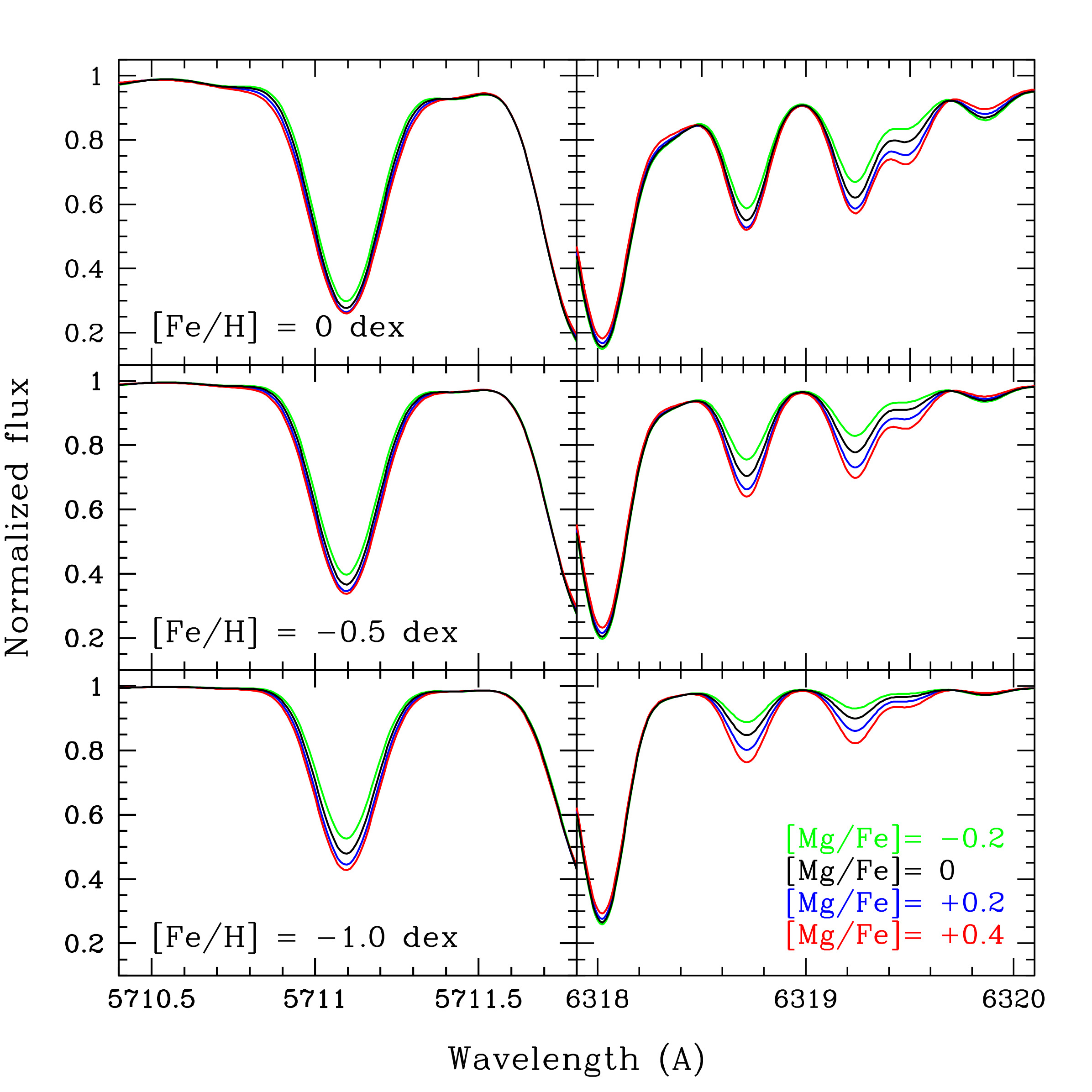
Figure 2: Synthetic spectra calculated for a representative giant star with $\rm T_{\rm eff}$ = 4200 K, log g = 1.00 and $\xi$ = 2.00 km/s at three different metallicities ([Fe/H]=–-1.0,–0.5,+0.0 dex, lower, middle and upper panels, respectively), around the Mg line at 5711 Å and the Mg triplet at 6318-19 Å (left and right panels, respectively). For each metallicity, synthetic spectra have been computed with different Mg abundances, namely [Mg/Fe]=–0.2 (green lines), =0.0 (black lines), +0.2 (blue lines) and +0.4 dex (red lines).

4.1 Error Estimates

Abundance uncertainties have been computed by summing in quadrature the error related to the measurement process and those arising from the adopted atmospheric parameters. The errors due to the measurement have been derived according to the method adopted to obtain the abundances.
Internal errors relative to the EW measurements have been estimated as the line-to-line scatter divided by the root mean square of the number of used lines. For the elements for which less than 4 lines are available (namely Al, Na, Y and Zr) we adopt the standard deviation from Fe I lines as more realistic estimate of the line-to-line scatter.
O, Mg, Sc, Co, V, Mn, Zn, Ba, La and Eu are the elements whose abundances are derived from spectral synthesis. The uncertainties of their measurement have been estimated by resorting to Monte Carlo simulation. We created synthetic spectra with representative values for the atmospheric parameters of the analysed stars, and we injected Poisson noise into them, according to the SNR of the observed spectra. For each line, 200 noisy spectra have been generated and the abundance derived adopting the same procedure used for observed spectra. Finally we calculated the internal measurement error as the standard deviation of the elemental abundance values derived from the 200 simulations.

The uncertainties arising from the atmospheric parameters have been computed by varying one only parameter at a time, keeping the other ones fixed, and deriving the abundance variation. This method provides a conservative estimate of the uncertainties because it does not take into account the correlations among the parameters. The applied variations are of 100 K, 0.1 dex, 0.1 km/s for $\rm T_{\rm eff}$  $\log g$ and $\xi$ respectively. The variations correspond to the typical uncertainties of the atmospheric parameters.

Since our results are expressed as abundance ratios, also the uncertainties in the Fe abundance have been taken into account. Therefore the final errors in [Fe/H] and [X/Fe] abundance ratios are calculated as follows:

$$\sigma_{[Fe/H]}=\sqrt{\frac{\sigma_{Fe}^{2}}{N_{Fe}}+(\delta^{\rm T_{\rm eff}}_{Fe})^{2}+(\delta^{log~{}g}_{Fe})^{2}+(\delta^{\eta}_{Fe})^{2}}$$ (1)

$$\sigma_{[X/Fe]}=\sqrt{\frac{\sigma_{X}^{2}}{N_{X}}+\frac{\sigma_{Fe}^{2}}{N_{Fe}}+(\delta^{\rm T_{\rm eff}}_{X}-\delta^{\rm T_{\rm eff}}_{Fe})^{2}+(\delta^{log~{}g}_{X}-\delta^{log~{}g}_{Fe})^{2}+(\delta^{\eta}_{X}-\delta^{\eta}_{Fe})^{2}}$$ (2)

where $\sigma_{X,Fe}$ is the dispersion around the mean of the chemical abundances, $N_{X,Fe}$ is the number of lines used to derive the abundances and $\delta^{i}_{X,Fe}$ are the abundance variations obtained modifying the atmospheric parameter i.

5 Results and discussion

This work provides for the first time a fully self-consistent comparison of the abundances for the main groups of elements (light-, $\alpha$-, iron-peak, neutron-capture elements) among the metal-rich stars in LMC, Sgr and MW. Although these samples cannot be considered as fully representative of the metallicity distributions of the parent galaxies, in particular because of some selection bias in their definition (see Section 2), this work has the main advantage to remove most of the systematics (i.e. solar abundances, atomic data, model atmospheres), affecting the comparison of their abundances.

Tables 2-4 list the measured values of the elemental abundances with their error. In Figs. 3-8 we show the results obtained for the three samples, together with the abundances in Galactic field stars from the literature (see caption of Figs. 3-8 for references). Only for the works that do not adopt solar values determined with their own linelist, we re-scaled their abundances to our solar reference values. The latter measures are shown as a sanity check to verify that our heterogeneous sample of MW stars reproduces the main MW chemical patterns. Also, the use of both dwarf and giant stars and of different assumptions in the chemical analyses (i. e. atomic data, solar reference values, model atmospheres, among others) could hamper the direct comparison with the LMC and Sgr abundances derived here. The comparison between our abundances and those from the literature is satisfactory for almost all the elements, while we found offsets of about 0.1-0.2 dex for Na, Al, Co, V and Eu. These differences are mainly explained by the different transitions, atomic parameters and (in the case of Na) NLTE corrections adopted by different authors. The existence of these offsets enforces the importance of a homogeneous analysis for all the stars.

In this section we also compare our results with the abundances available in literature, i.e. Pompéia et al. (2008), Lapenna et al. (2012), Van der Swaelmen et al. (2013), Nidever et al. (2020) for the LMC and Monaco et al. (2005), Sbordone et al. (2007), Carretta et al. (2010) and Mucciarelli et al. (2017a) for Sgr.

5.1 Light elements: Na and Al

Na and Al are mainly synthesized in massive stars through the hydrostatic C and Ne burning and only a small amount is produced during the H burning through the NeNa and MgAl cycles in AGB stars (Woosley & Weaver, 1995). Stars in the LMC and Sgr have similar [Na/Fe] and [Al/Fe] abundance ratios that are significantly lower (by  0.5 dex) than those measured in the MW sample (Fig. 3). These low values could suggest that the contribution by massive stars is similar in the two galaxies but significantly lower than that in the MW.

Low [Al/Fe] and [Na/Fe] abundances have been measured in Sgr stars also by Sbordone et al. (2007) and McWilliam et al. (2013), even if there are an offset of about -0.2 dex for Al and +0.3 dex for Na with respect to our values that are likely attributable to the different log gf (as in the case of Al) or NLTE corrections (as in the case of Na). Instead, the Sgr stars analysed by Carretta et al. (2010) exhibit higher [Na/Fe] values. This difference can be only partially explained by the different NLTE corrections for the Na lines.

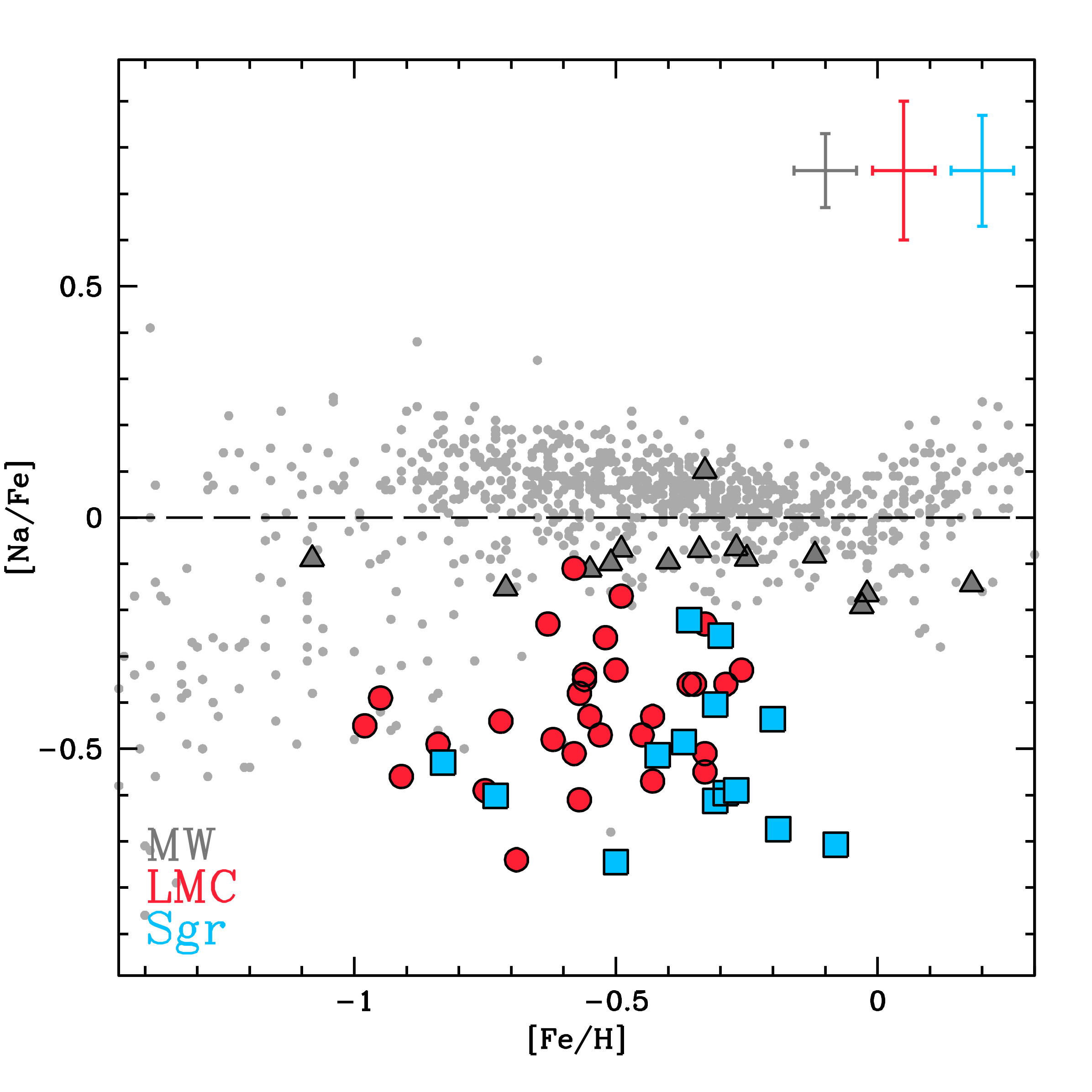
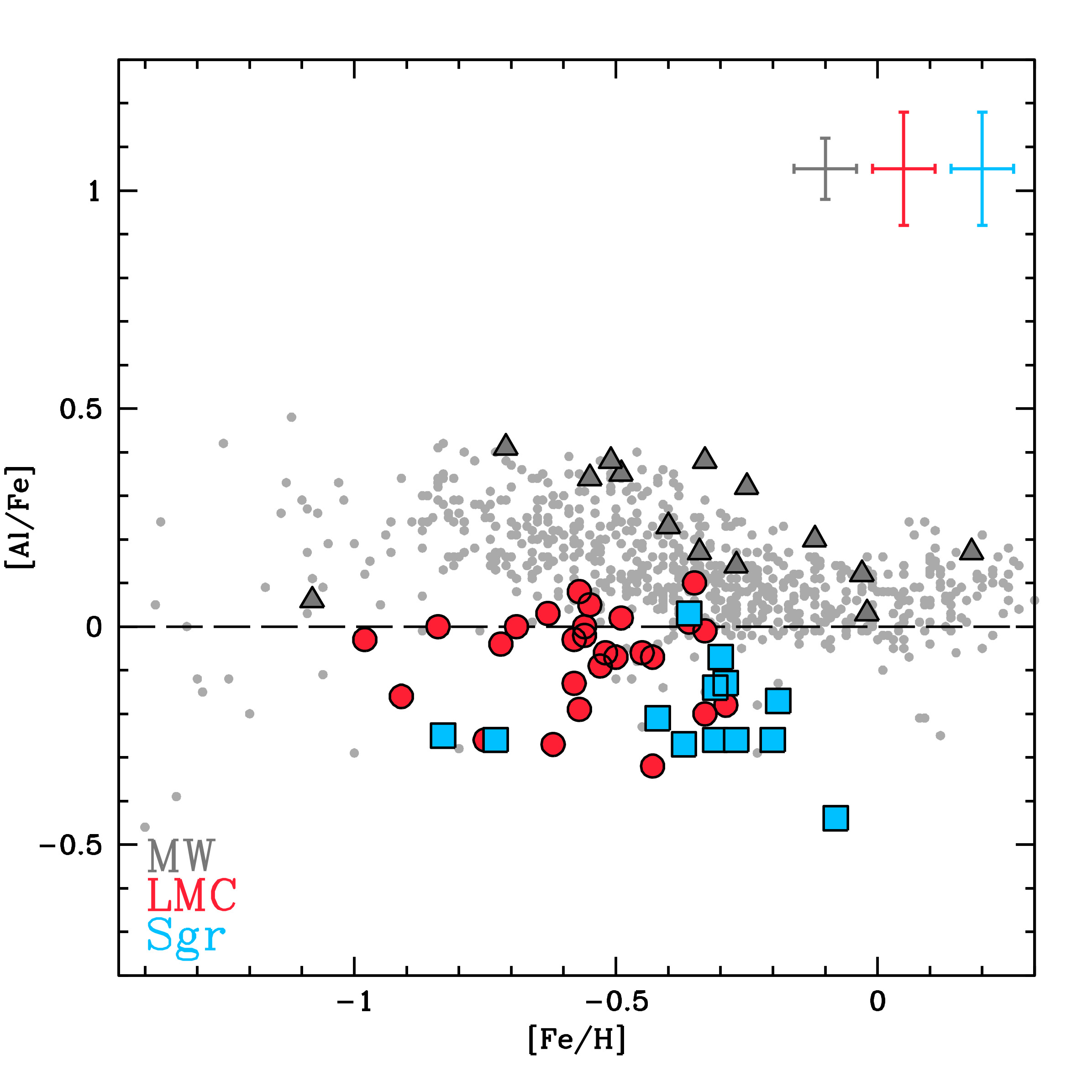
Figure 3: Behavior of the light elements [Na/Fe] and [Al/Fe] abundance ratios (left and right panel, respectively) as a function of [Fe/H] for LMC sample (red circles), Sgr sample (light blue squares) and MW sample (gray triangles). Abundances of Galactic stars from the literature are also plotted as a reference: Edvardsson et al. (1993); Fulbright (2000); Reddy et al. (2003, 2006); Bensby et al. (2005) for both the elements, and Stephens & Boesgaard (2002); Gratton et al. (2003) for Na.

5.2 $\alpha$-elements

The $\alpha$-elements are mainly produced in short-lived massive stars and released in the interstellar medium through SNe II, with only a minor component produced in SN Ia that produce, instead, significant amounts of Fe on long timescales. Therefore, [$\alpha$/Fe] ratios are used to trace the time-scales of the star formation in a given environment (Tinsley, 1979; Matteucci & Brocato, 1990; Gilmore & Wyse, 1991). We grouped the measured $\alpha$-elements according to their formation mechanism: hydrostatic elements (O and Mg) that are synthesized via hydrostatic C and Ne burning, mainly in stars with masses larger than 30-35 $\rm M_{\odot}$ and without contributions by SN Ia, and explosive elements (Si, Ca and Ti) that are synthesized via explosive O and Si burning, mainly in stars with masses of 15-25 $\rm M_{\odot}$ (Woosley & Weaver, 1995), and in a smaller amount in SN Ia.

Fig. 4 shows the behavior of the average abundance ratios of the two groups as a function of [Fe/H]. For both groups of elements, LMC and Sgr agree each other but with values of [$\alpha$/Fe] lower than those measured in MW stars of similar [Fe/H]. This difference is more pronounced for the hydrostatic $\alpha$-elements. Also, the hydrostatic $\alpha$-elements show a clear decrease with increasing [Fe/H], reaching sub-solar values at [Fe/H]$>$–0.6 dex, at variance with the explosive elements that display a less pronounced decrease by increasing [Fe/H]. It is worth noticing that most of the Sgr stars have [Fe/H]$>$–0.5 dex and only two stars with [Fe/H] between –1.0 dex and –0.5 dex are in the Sgr sample. However, the abundance ratios for these two stars well match with those of the LMC stars of similar [Fe/H].

The low [$\alpha$/Fe] ratios measured in LMC/Sgr point out that these stars formed from a gas already enriched by SN Ia at [Fe/H]$>$–1 dex. Also, the larger difference between LMC/Sgr and MW measured for hydrostatic $\alpha$-elements is consistent with galaxies having a lower number of stars more massive than $\sim$30 ${\rm M_{\odot}}$, for instance galaxies with a lower star formation efficiency (like LMC and Sgr).
Comparing our abundances with the literature, no significant differences are found between the $\alpha$ abundances in the LMC sample and the ones derived by Pompéia et al. (2008), Lapenna et al. (2012) and Van der Swaelmen et al. (2013). Concerning Sgr, we find a general good agreement with the Mg, Ca and Ti abundances by Monaco et al. (2005) and with the Mg and Ca abundances by Mucciarelli et al. (2017a). A nice agreement is found also with the abundances by Sbordone et al. (2007) but Ti that is lower than our values by $\sim$0.3/0.4 dex, likely due to the large sensitivity of the Ti abundance to $\rm T_{\rm eff}$. Our O, Si and Ti abundances match those by Carretta et al. (2010), while their Mg are higher than ours by $\sim$0.3 dex, likely due to their selected Mg lines (see Section 4). Finally, we highlight the different behavior found by Nidever et al. (2020) that measured Mg, Si and Ca abundances from near-infrared APOGEE spectra of LMC giant stars. In their sample the [$\alpha$/Fe] ratios show a flat run with [Fe/H], compatible with our result for Si and Ca but clearly different concerning Mg. The O and Mg abundances in our MW sample are slightly higher by $\sim$0.15 dex than the literature data. We ascribe this difference to the different O and Mg lines used in the literature that are mainly based on dwarf stars. Because O and Mg abundances are derived by a few lines in both dwarf and giant stars, differences in the used diagnostics (in terms of the zero-point of their gf values or NLTE effects) are particularly evident for these elements. This difference between the abundances of our MW sample and the literature highlights again the importance of a homogeneous analysis.

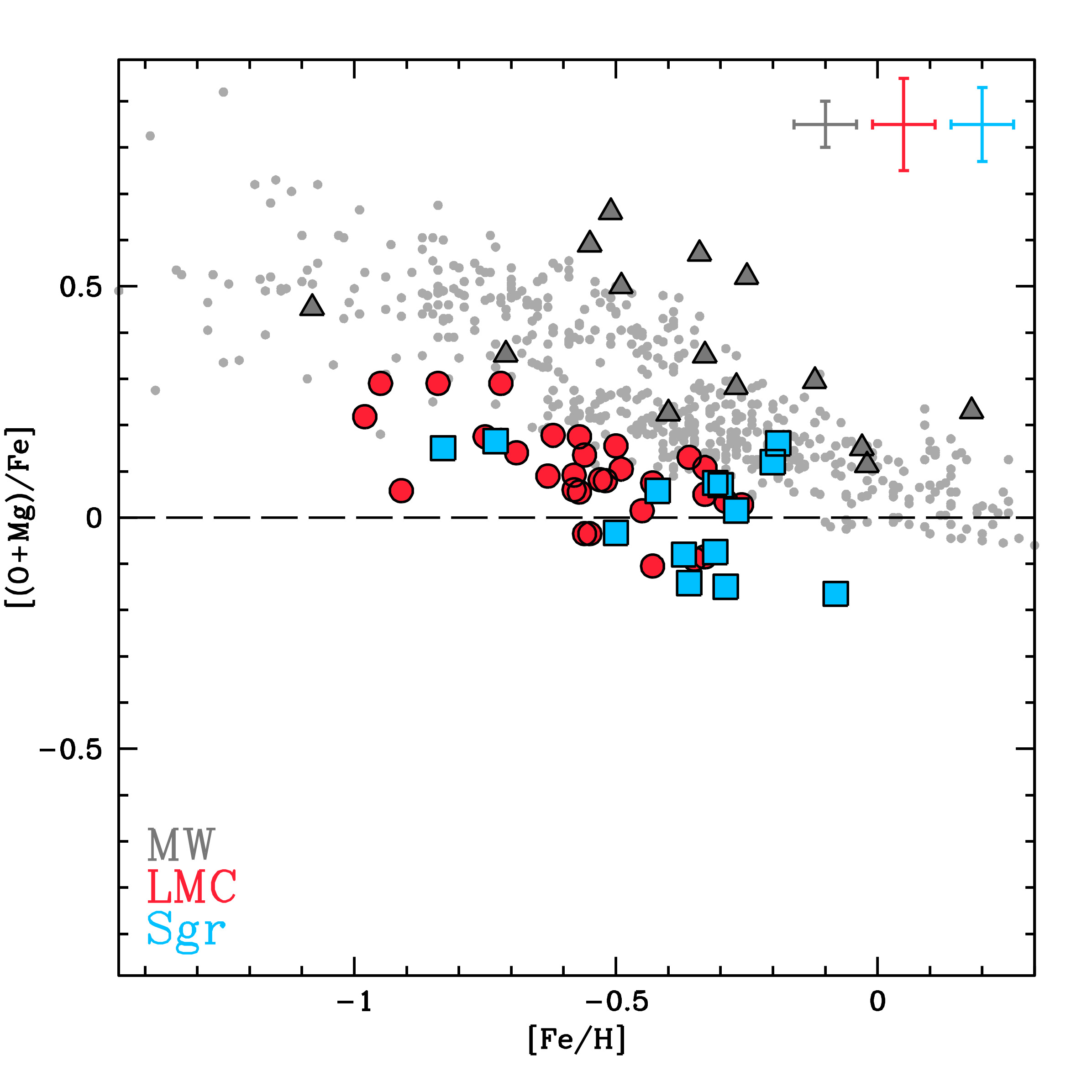
Figure 4: Behavior of the hydrostatic and explosive [$\alpha/Fe]$ abundance ratio (left and right panel, respectively) as a function of [Fe/H]. Same symbols of Fig. 3. The MW literature data for both groups of elements are from Edvardsson et al. (1993); Gratton et al. (2003); Reddy et al. (2003, 2006); Bensby et al. (2005), while for the explosive elements additional data are from Fulbright (2000); Stephens & Boesgaard (2002); Barklem et al. (2005).

5.3 Iron-peak elements

The iron-peak elements are the heaviest elements synthesized through thermonuclear reactions. They compose an heterogeneous group of elements in terms of nucleosynthesis. They form partly in massive stars, sometimes with a significant contribution by HNe (that are associated to stars more massive than $\sim$25-30 $M_{\odot}$ and more energetic by at least one order of magnitude with respect to normal SNe II). Not negligible amounts of Fe-peak elements can be produced also in SNe Ia (Leung & Nomoto, 2018, 2020; Lach et al., 2020). Moreover, further complicating matters, some of the iron-peak elements have a strong dependence of their yields on the metallicity (see e.g. Romano et al., 2010).

LMC and Sgr stars exhibit similar abundance patterns for all the measured iron-peak elements, as shown in Fig. 5.

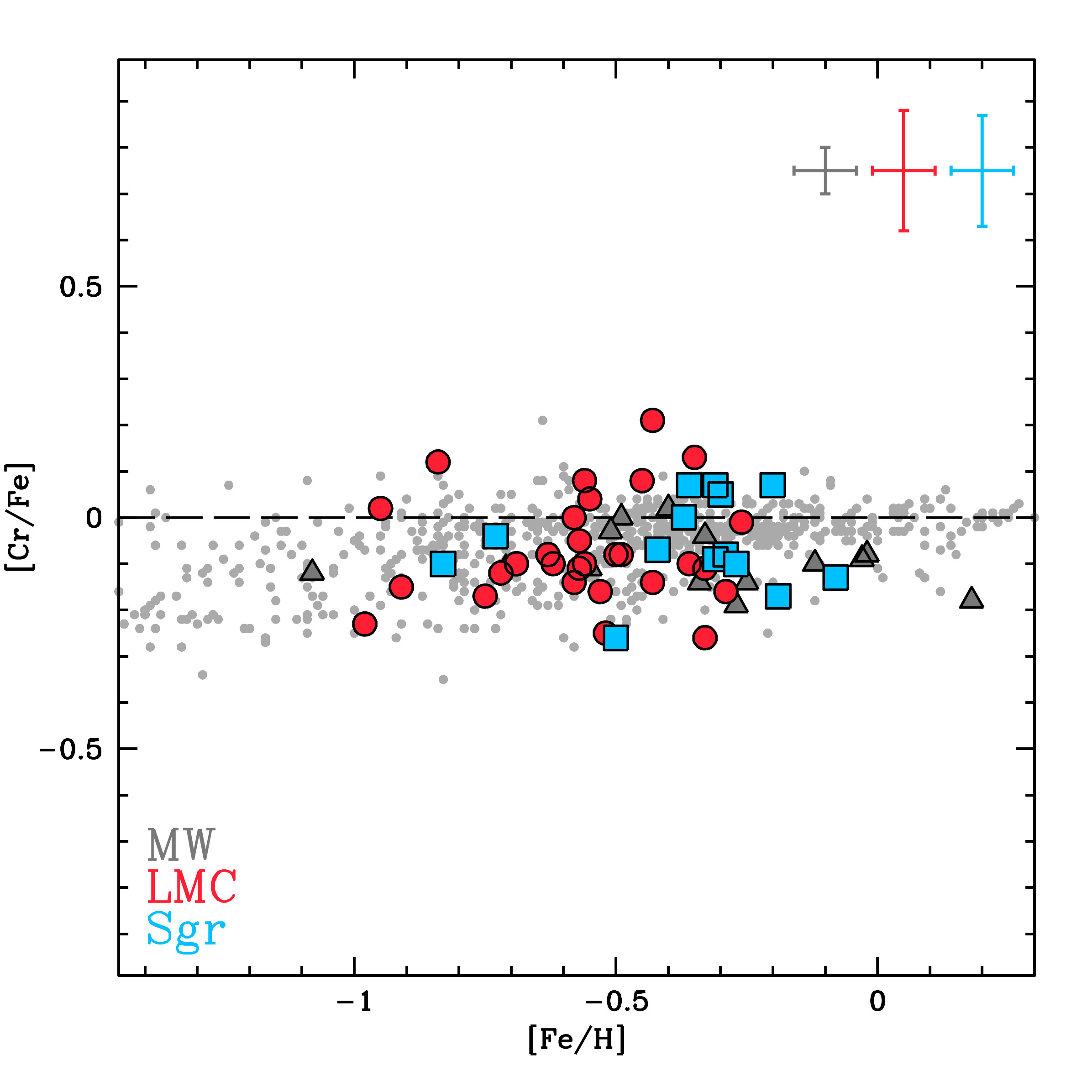
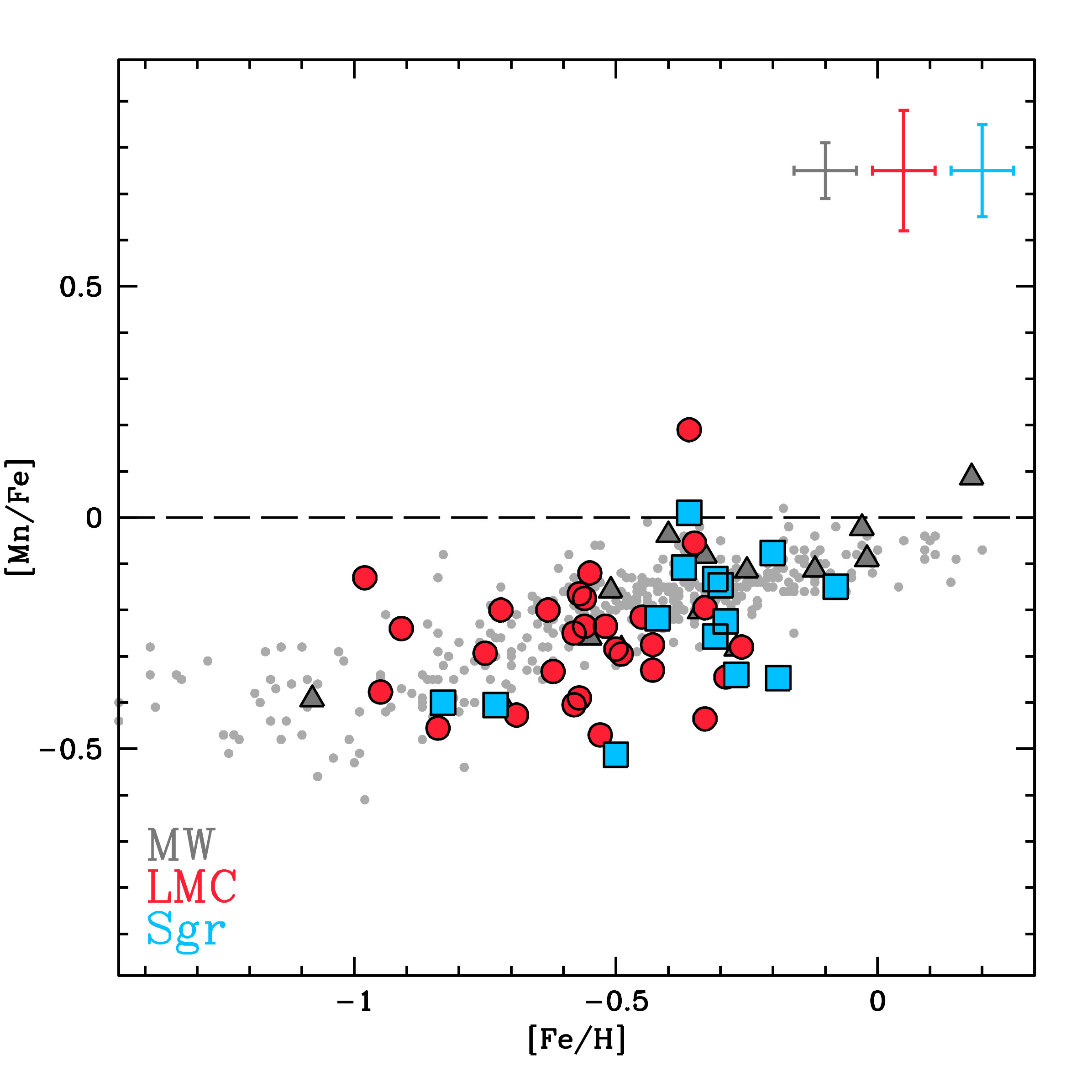
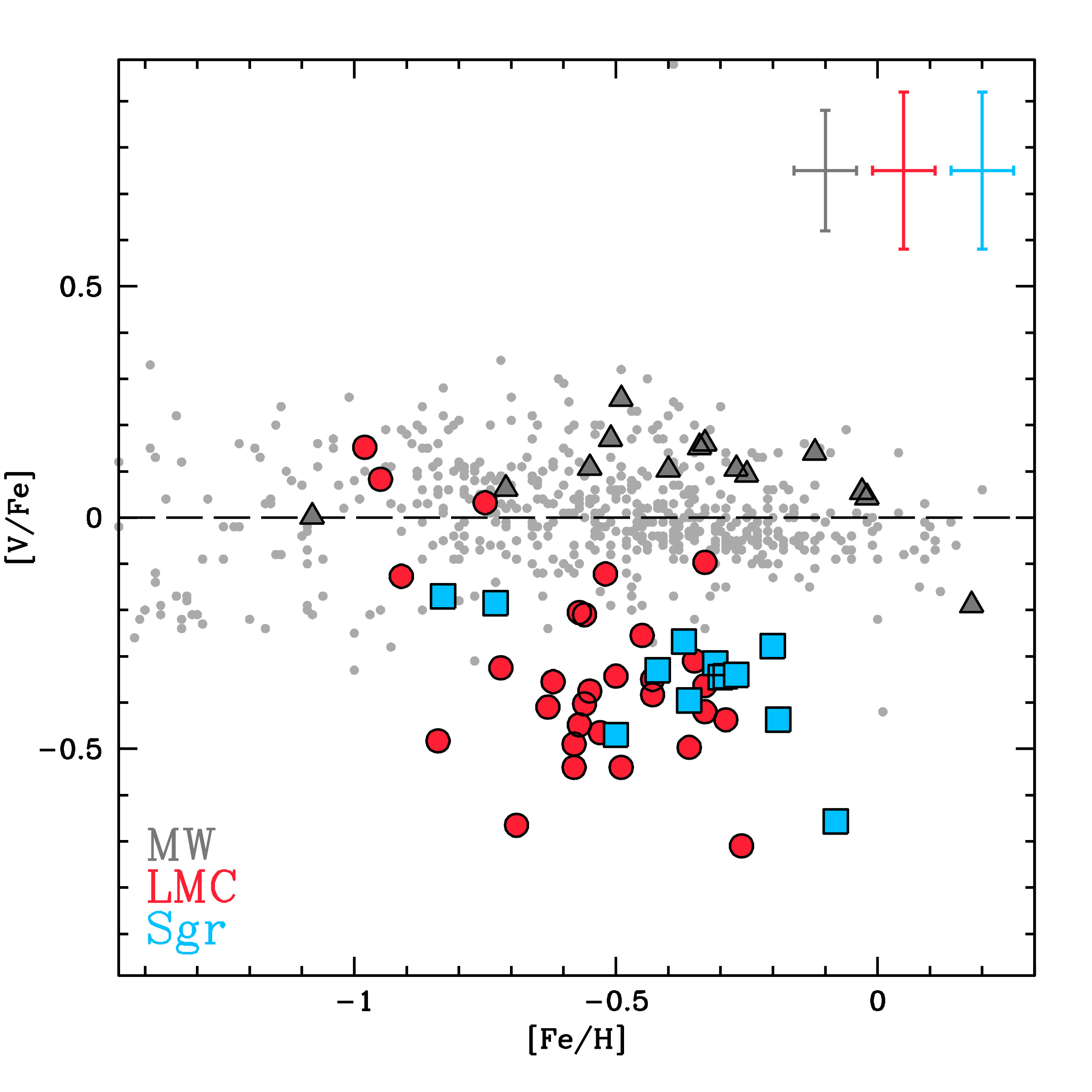
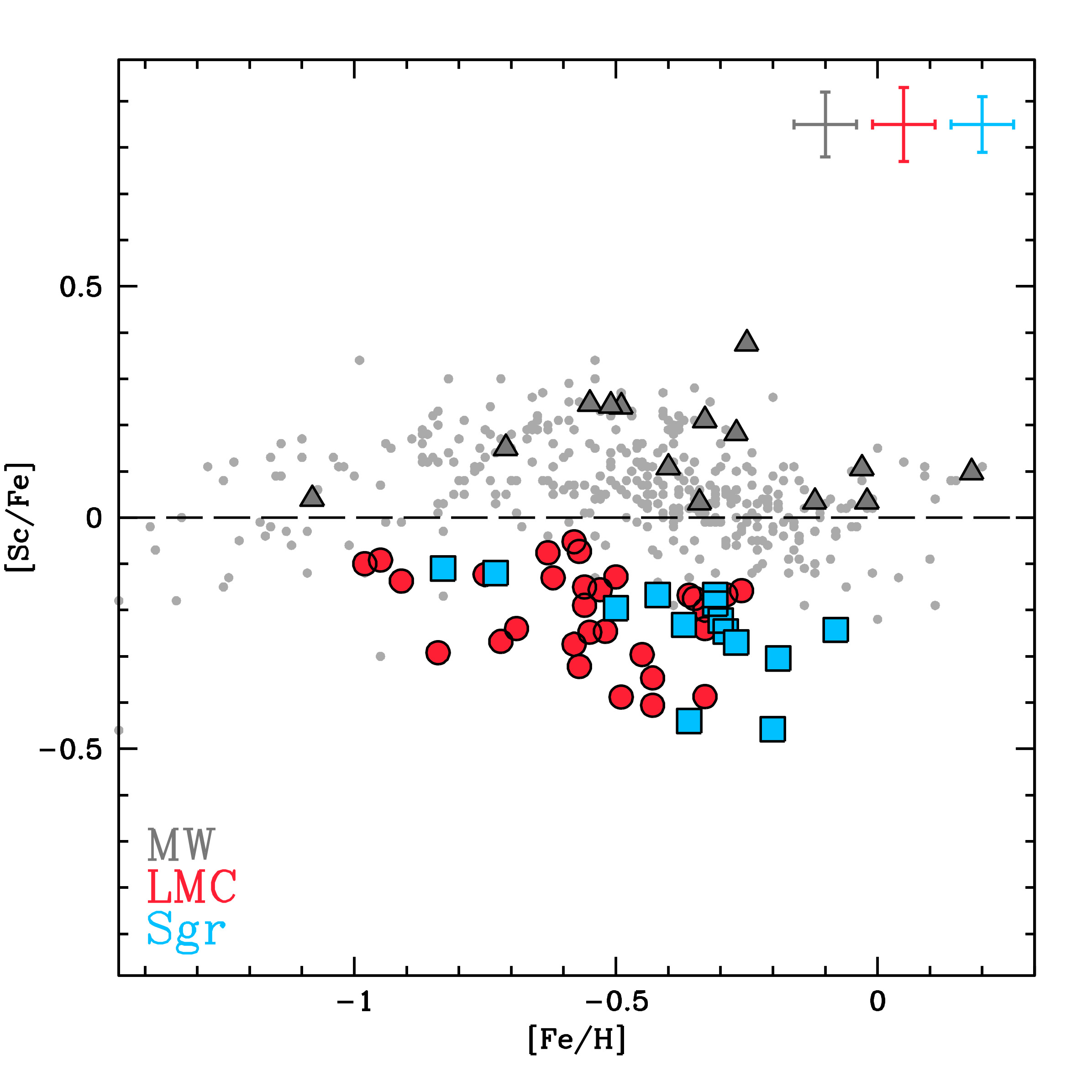
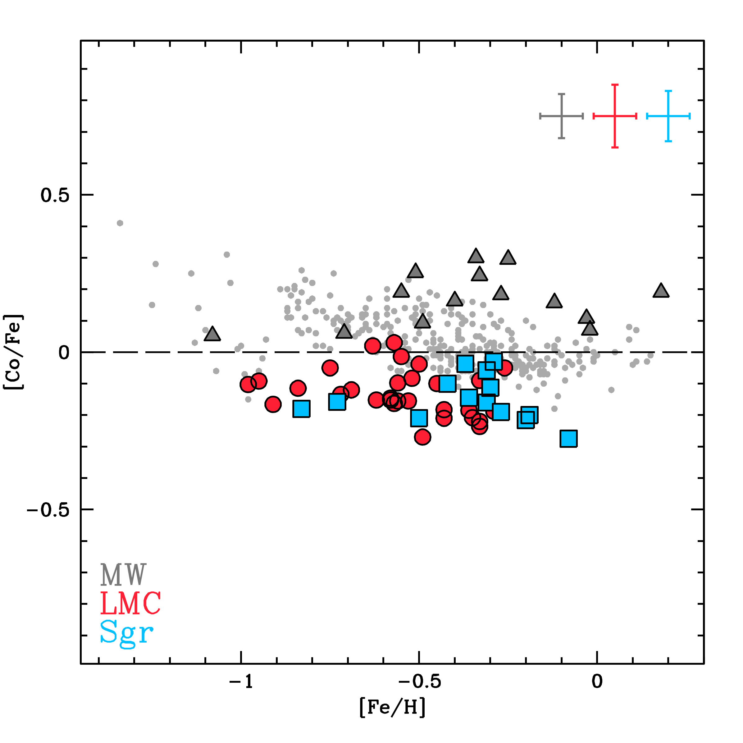
Figure 5: Behavior of the iron-peak [Cr/Fe], [Mn/Fe], [V/Fe], [Zn/Fe], [Co/Fe], [Ni/Fe] and [Sc/Fe] abundance ratios as a function of [Fe/H]. Same symbols of Fig. 3. The MW literature data are from the works of Edvardsson et al. (1993)(Ni), Fulbright (2000) (V, Cr, Ni), Stephens & Boesgaard (2002)(Cr, Ni), Gratton et al. (2003) (Sc, V, Cr, Mn, Ni, Zn), Reddy et al. (2003, 2006) (Sc, V, Cr, Mn, Co, Ni, Zn), Bensby et al. (2005)(Cr, Ni, Zn), Nissen et al. (2007)(Zn)

Differences with respect to the MW stars are evident for Sc, V, Co, Ni and Zn abundances, showing in the cases of [Sc/Fe] and [Ni/Fe] a clear decrease of the abundance ratios by increasing [Fe/H]. A decreasing trend is also seen in [Zn/Fe] for the LMC sample, but the small number of Sgr stars with Zn measures prevents to properly identify a possible trend with [Fe/H].

The largest differences are observed for [V/Fe] and [Zn/Fe], whose values in LMC/Sgr stars are lower by 0.5-0.7 dex respect to MW stars of similar metallicity. In contrast, [Cr/Fe] and [Mn/Fe] show values comparable between LMC/Sgr and MW stars.
Even if the details of the nucleosynthesis of these elements are not fully known and for some of them the current evolutionary chemical models are not even able to reproduce the observed MW trends (Romano et al., 2010), the chemical patterns obtained for the three samples provide a scenario coherent with that drawn above based on the abundances of light and $\alpha$-elements. In fact, a large amount of these elements is produced by massive stars, via SNe II, HNe and electron-capture SNe. The measured abundances in LMC and Sgr stars for most of the iron-peak elements are compatible with a scenario where the contribution by massive stars to the chemical enrichment of the parent galaxies is less important than in the MW. In particular, the low abundances of Zn would suggest a small or lacking contribution by stars more massive than $\sim$25-30 $M_{\odot}$, because this element is almost totally produced by HNe (Nomoto et al., 2013), while its production in SNe Ia is probably negligible.

As noted above, V and Zn exhibit the largest differences with respect to the MW stars with similar [Fe/H]. These abundance ratios are the most clean-cut chemical differences between LMC/Sgr and MW and in principle they could be used to distinguish, among the MW stars with [Fe/H]$>$–1 dex, those formed in smaller satellites that evolved similarly to the LMC/Sgr and were subsequently accreted and disrupted by the MW tidal field. Zn abundances lower than those in MW stars of similar metallicity have been measured also in Sculptor (Skúladóttir et al., 2017) and in other dwarf galaxies (Shetrone et al., 2001, 2003), but at lower metallicities than those discussed here.

5.4 Slow neutron-capture elements

Elements heavier than Fe are produced through neutron capture processes on seed nuclei (Fe and iron-peak elements), and subsequent $\beta$ decays (Burbidge et al., 1957). According to the rate of neutron captures with respect to the time-scale of the $\beta$ decays, we distinguish slow (s-) and rapid (r-)process elements. The s-process elements are grouped around three peaks of stability corresponding to the neutrons magic numbers (N=50, 82, 126). These elements are produced mainly by low-mass (1-3 $M_{\odot}$) AGB stars (whose yields are strongly metallicity dependent) with only a minor component produced in massive stars (see e.g. Busso et al., 1999).

We measured Y and Zr abundances among the elements belonging to the first-peak. The elements of this group are produced mainly in AGB stars with high metallicity, because the decrease of the number of neutrons per seed nucleus favors the formation of the lightest s-process elements (ls). As shown in the first two panels of Fig. 7, the three samples overlap each other, even if the large scatter, particularly in [Y/Fe] among the LMC and Sgr stars, makes it hard to compare these samples with the MW.
For the second peak, the heavy s-process elements (hs), we measured Ba, La (that are produced mainly through s-process) and Nd (that is produced by s-process for nearly 40% of the total, see e.g. Arlandini et al., 1999). The abundance behavior for these elements is illustrated in the corresponding panels of Fig. 7. Both in LMC and Sgr their abundance ratios are enhanced and higher than those measured in the MW stars, with the Sgr stars that show abundances higher than the LMC stars. The Sgr stars with [Fe/H]$<$–0.4 dex have [hs/Fe] compatible with those measured in LMC stars, while at higher [Fe/H] these abundance ratios increase significantly, reaching values of about +1 dex. In Fig. 6 we show the profile of the Zr and Ba lines in two pairs of LMC/Sgr stars with similar parameters and metallicity: the stars in the upper panel have similar Zr and Ba abundances, as demonstrated by their similar line strengths, while the the Sgr star shown in the lower panel exhibit Zr and Ba lines stronger than the those of the LMC star with similar parameters and metallicity.
The high heavy s-process element abundances measured in the most metal-rich Sgr stars seem to suggest a more significant contribution by metal-rich AGB stars in Sgr with respect to LMC. Also, LMC/Sgr stars have abundances of [hs/Fe] higher than those measured in the MW, where the enhancement is moderate .

Our abundances agree with those measured by Van der Swaelmen et al. (2013) for LMC stars and by Sbordone et al. (2007) for Sgr stars, despite some offsets due to the adopted atomic data.

In the last panel of Fig. 7 we plot the heavy-to-light s-process abundance ratios as a function of [Fe/H] in order to evaluate the relative contribution of the two groups of s-process elements that mainly arise from AGB stars of different metallicity. All the three galaxies shows an increase of this ratio by increasing [Fe/H] with a trend that is steeper in LMC and Sgr. This behaviour points out that the production of s-process elements in these two galaxies is dominated by AGB stars more metal-poor than in the MW. On the other hand, the production of heavy s-process elements is favored in less massive AGB stars, while elements of the first peak are produced in a similar amount in AGB stars regardless of their mass (see AGB models of Lugaro et al., 2012; Karakas & Lattanzio, 2014). Hence, the higher [hs/ls] ratios observed in LMC and Sgr with respect to the MW could suggest a lower contribution by the most massive AGB stars.

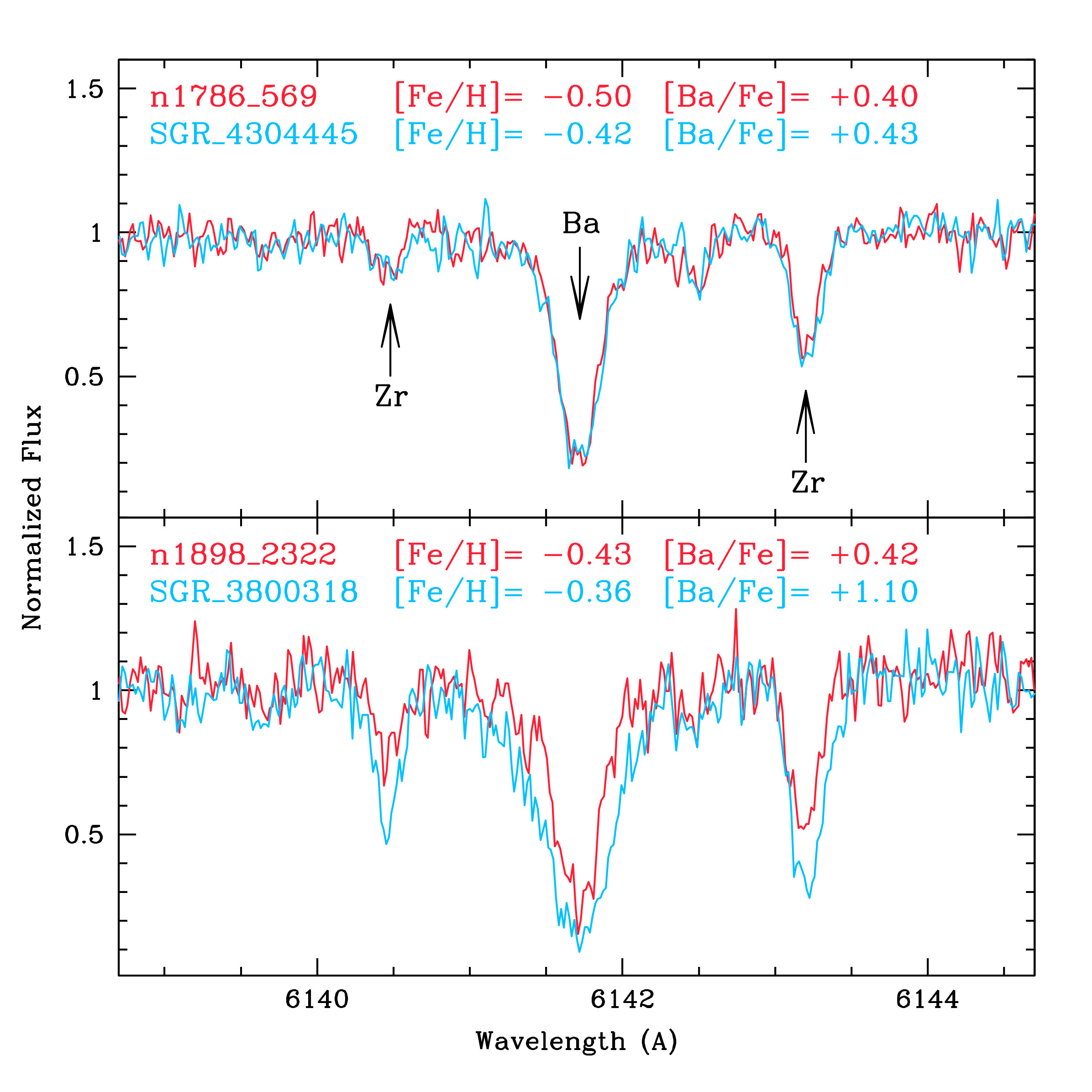
Figure 6: Comparison between the spectra of the two pairs of LMC and Sgr stars (red and blue lines, respectively) with similar stellar parameters and metallicities around the Ba II line at 6142 Å . The upper panel shows the comparison between two stars with similar Ba abundances (two Zr lines are also visible in the spectral range), while the lower panel shows the comparison between two stars characterized by a strong difference in both Zr and Ba abundances.

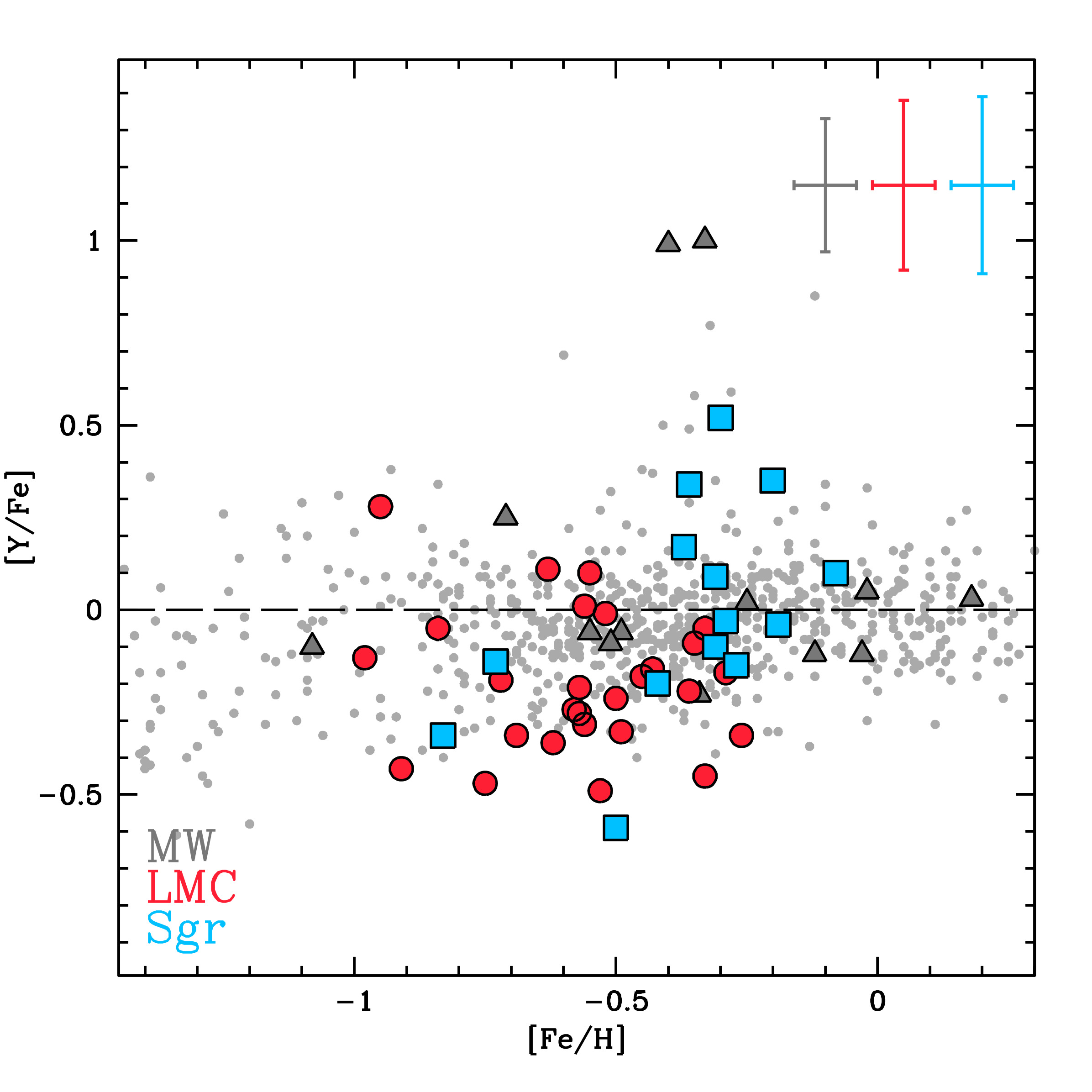
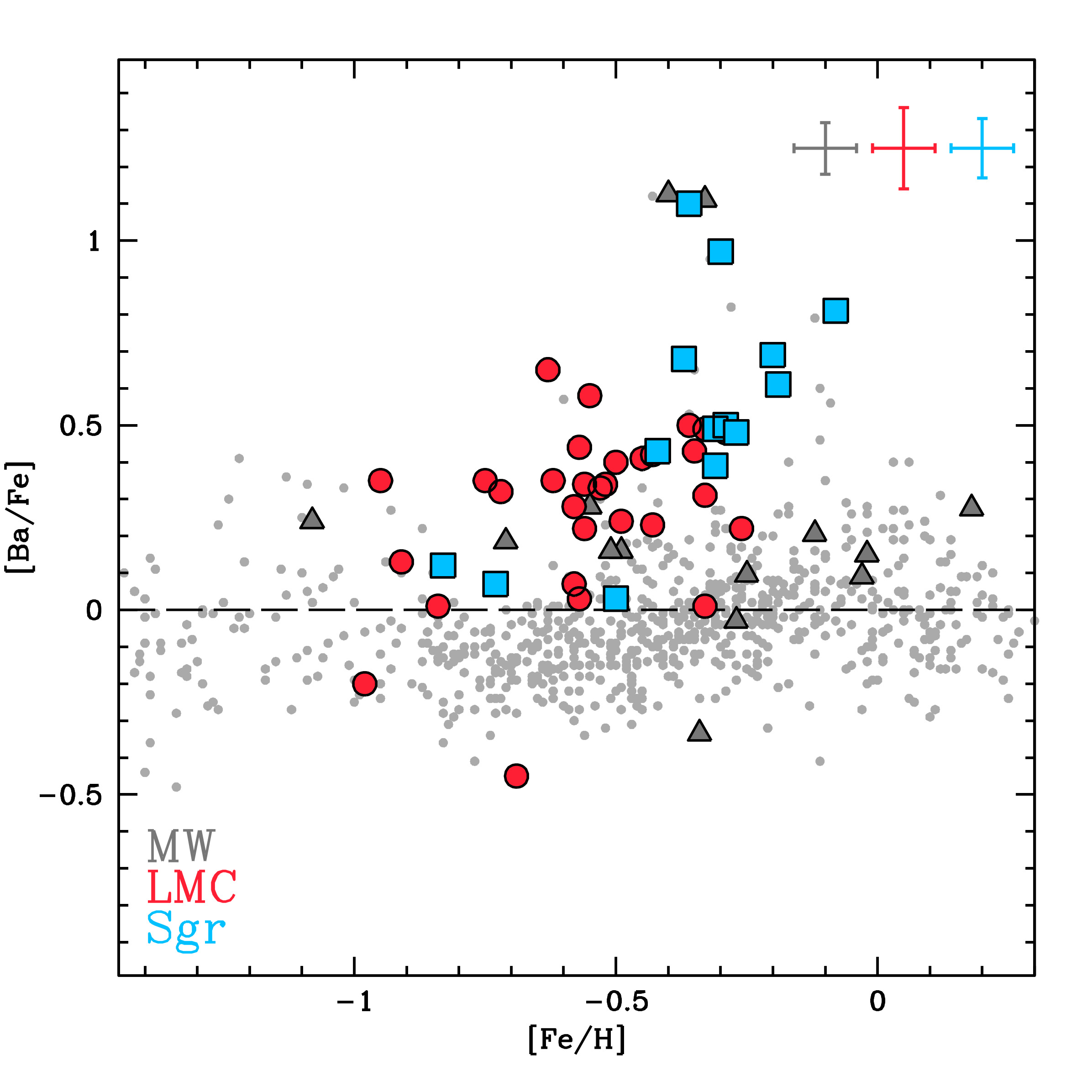
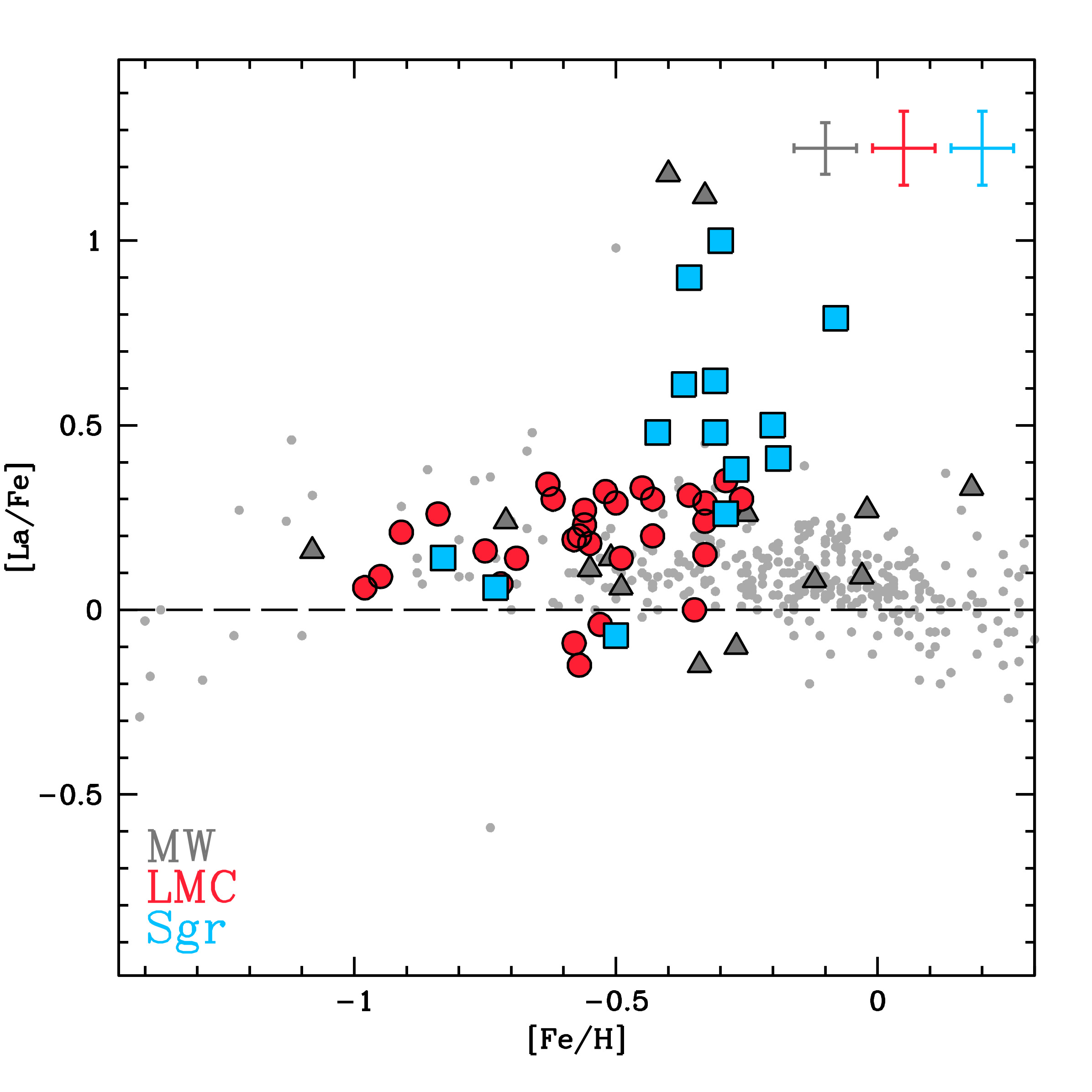
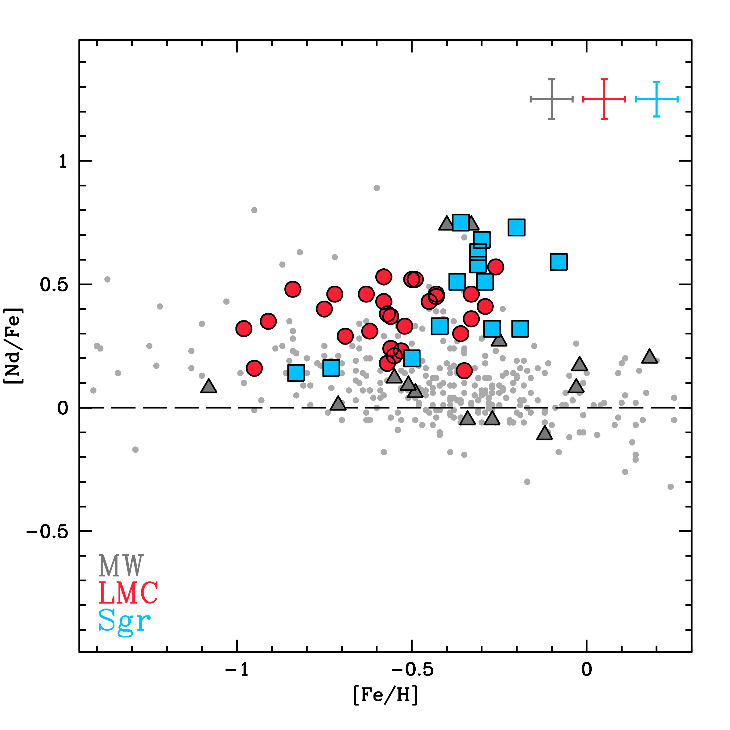
Figure 7: Behavior of the slow neutron-capture [Y/Fe], [Zr/Fe], [Ba/Fe], [La/Fe] and [Nd/Fe] as a function of [Fe/H]. In the last panel the comparison between ls and hs elements, where the ratio between the average value of Ba and La and the average value of Y and Zr is represented as a function of [Fe/H]. Same symbols of Fig. 3. The MW literature data are from Edvardsson et al. (1993, Y, Zr, Ba, Nd), Burris et al. (2000, Y, Zr, Ba, La, Nd), Fulbright (2000, Y, Zr, Ba), Stephens & Boesgaard (2002, Y, Ba), Reddy et al. (2003, Y, Zr, Ba, Nd), Reddy et al. (2006, Y, Ba, Nd), Barklem et al. (2005, Ba), Bensby et al. (2005, Y, Ba), Forsberg et al. (2019, Zr, La).

5.5 Rapid neutron-capture elements

Rapid neutron-capture processes produce an half of the heaviest elements (see e.g. the seminal paper by Burbidge et al., 1957) but their precise sites of production are still debated, requiring neutron-rich, high energy environments. Among the possible sites, the most promising are low-mass SNII progenitors (in the range 8-10 $M_{\odot}$ see e.g. Wheeler et al., 1998), the neutron star mergers (Pian et al., 2017) and the collapsars (Siegel et al., 2019). We measured the abundance of Eu that is an almost pure r-process element.

As shown in the last panel of Fig. 8, both LMC and Sgr exhibit enhanced values of [Eu/Fe], comparable with those of the MW. The enhancement of [Eu/Fe] in LMC and Sgr in this range of metallicity has been already measured in previous works in a few stars (Bonifacio et al., 2000; Van der Swaelmen et al., 2013; McWilliam et al., 2013). A possible decrease of [Eu/Fe] by increasing [Fe/H] is visible among the LMC stars, while the same pattern is not clearly visible in Sgr. Comparable enhanced values of [Eu/Fe] in the three samples seem to suggest a similar production of r-process elements in these galaxies, in particular a similar rate of neutron star mergers per unit stellar mass, if neutron star mergers are the main contributors to the Galactic Eu abundances (see e.g. Matteucci et al., 2014).

Finally, we evaluate the abundance ratio between heavy s-process elements (considering the average of Ba and La abundances) and Eu, in order to estimate the contribution of the r-process to the production of other neutron-capture elements. As shown in the last panel of Fig. 8, [hs/Eu] exhibits a rapid increase by increasing [Fe/H] in all the three samples and in LMC/Sgr this increase occurs at lower metallicities that the MW. Theoretical models by Arlandini et al. (1999) and Burris et al. (2000) predict values of [Ba/Eu] of about –0.5 dex in case of pure r-process. The measured [hs/Fe] abundance ratios suggest that the role played by the r-process to the production of Ba and La decreases by increasing [Fe/H] and that in the metal-rich stars of LMC and Sgr the production of Ba and La is dominated by s-processes.

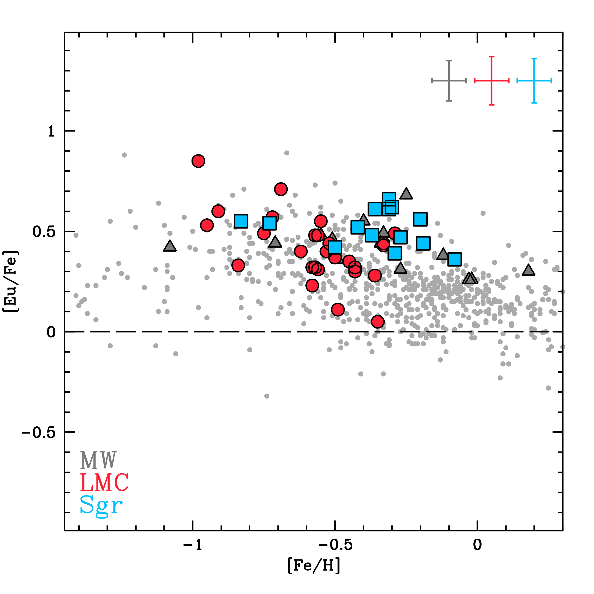
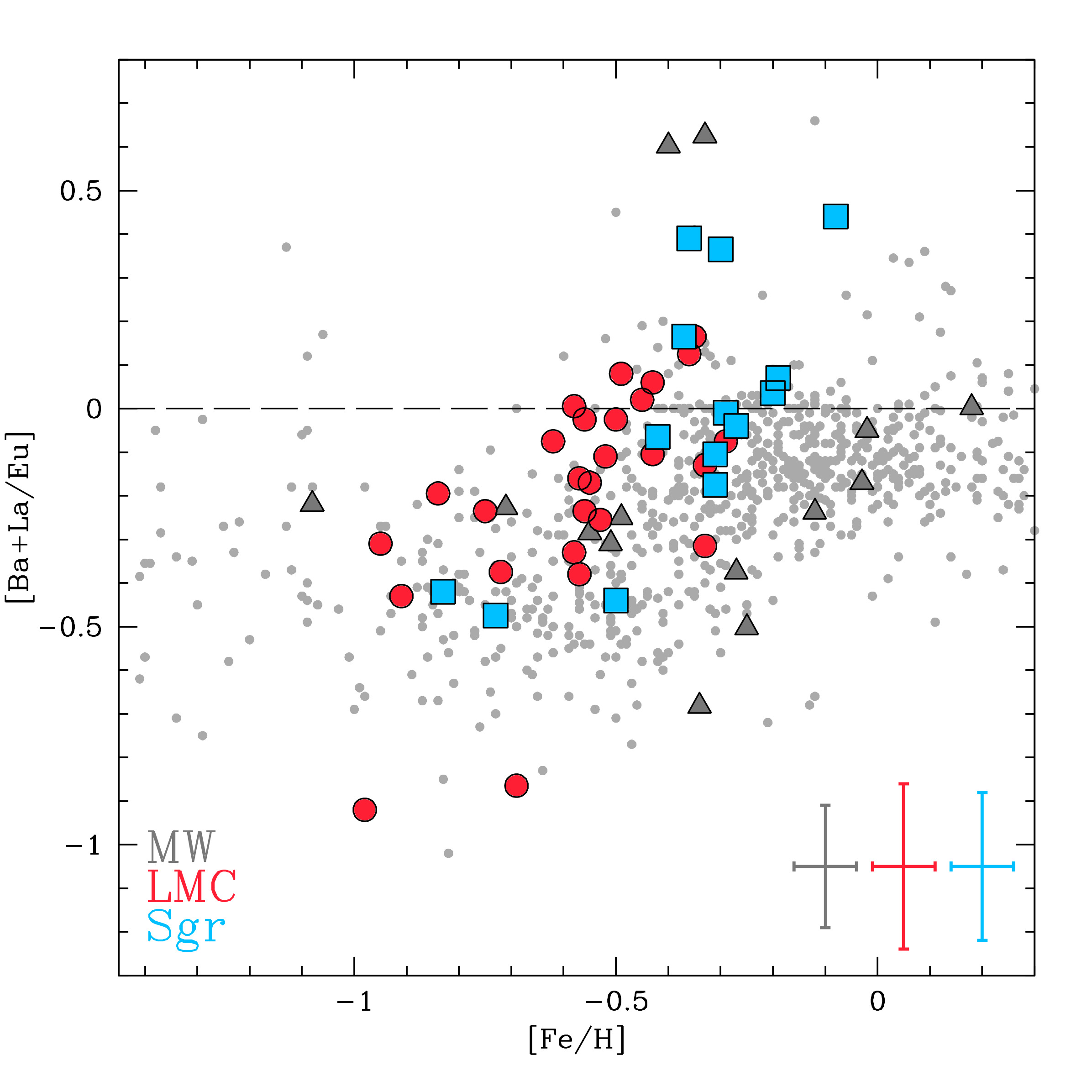
Figure 8: In the left panel, behavior of the [Eu/Fe] abundance ratio as a function of [Fe/H]. In the right panel, the ratio between the hs elements (average value between Ba and La abundances) and the Eu abundances, as a function of [Fe/H]. Same symbols of Fig. 3. The MW literature data are from Burris et al. (2000); Fulbright (2000); Reddy et al. (2003, 2006); Barklem et al. (2005); Bensby et al. (2005); Forsberg et al. (2019) for Eu.

6 Conclusions

High-resolution UVES-FLAMES spectra of 30 LMC and 14 Sgr giant stars have been analysed, together with a reference sample of 14 MW giant stars selected in the same metallicity range of the LMC/Sgr stars. The three samples have been analysed with the same procedure in order to erase the main systematics of the analysis (such as solar reference abundances, atomic data, temperature scales among others). The homogeneous analysis of different samples of stars is a necessary step to highlight differences and similarities in the chemical compositions of these three galaxies.

The metal-rich populations in LMC and Sgr show strong similarities in almost all the measured species, pointing out a similar chemical evolution. The main differences are related to the heavy s-process elements Ba and La, with the stars of Sgr more enriched in both the abundance ratios with respect to LMC, suggesting a different contribution by AGB stars. Overall, their similar chemical compositions suggest similar chemical enrichment histories, coherently with a scenario where the progenitor of Sgr was a galaxy with a mass and a star formation rate similar to those of the LMC, as already suggested by different authors (see e.g. de Boer et al., 2014; Gibbons et al., 2017; Mucciarelli et al., 2017a).

The comparison between LMC/Sgr and MW samples reveals that the former galaxies have different chemical abundances with respect to the MW stars for almost all the species. This finding agrees with previous works about metal-rich stars in LMC (Pompéia et al., 2008; Lapenna et al., 2012; Van der Swaelmen et al., 2013) and Sgr (Monaco et al., 2005; Sbordone et al., 2007; Mucciarelli et al., 2017a) but we stress that the present work is the first that allows to directly compare the abundances of all the main groups of elements in these galaxies. The abundance ratios for elements produced by massive stars exploding either as core-collapse SNe or HNe are systematically lower in LMC/Sgr with respect to the MW, pointing out that in these galaxies the contribution by massive stars to the chemical enrichment is less important. This can be explained in light of their low star formation rates, leading to a lower number of massive stars (poorly populating the IMF at the highest masses, see e.g. Yan et al., 2017; Jeřábková et al., 2018) and penalizing the elements produced by very massive stars.

Finally, we recall that, among the measured elements, the most evident differences between LMC/Sgr and MW stars are measured for [V/Fe] and [Zn/Fe], where LMC/Sgr stars have abundance ratios lower than the MW stars of similar metallicity by as much as 0.5-0.7 dex. We suggest that these abundance ratios can be used to identify possible extra-galactic interlopers among the Galactic disk stars with [Fe/H]$>$–1.0 dex, i.e. stars accreted from LMC and Sgr or from galaxies that have experienced similar chemical enrichment histories. In other words, we suggest that [V/Fe] and [Zn/Fe] can be tools for a robust chemical tagging as powerful as the classical hydrostatic [$\alpha$/Fe] ratios.

Table 2: LMC and Sgr chemical abundances

ID	[$\frac{Fe}{H}$]	err	[$\frac{FeII}{H}$]	err	[$\frac{Na}{Fe}$]	err	[$\frac{Al}{Fe}$]	err	[$\frac{O}{Fe}$]	err	[$\frac{Mg}{Fe}$]	err	[$\frac{Si}{Fe}$]	err	[$\frac{Ca}{Fe}$]	err	[$\frac{Ti}{Fe}$]	err	[$\frac{Sc}{Fe}$]	err	[$\frac{V}{Fe}$]	err
LMC
NGC1754_248	-0.53	0.06	-0.56	0.22	-0.47	0.14	-0.09	0.14	0.25	0.06	-0.08	0.20	0.23	0.10	-0.03	0.13	-0.11	0.17	-0.16	0.05	-0.46	0.17
NGC1786_2191	-0.29	0.05	-0.31	0.16	-0.36	0.08	-0.18	0.08	0.14	0.06	-0.07	0.06	0.08	0.10	-0.04	0.05	-0.18	0.12	-0.17	0.07	-0.44	0.16
NGC1786_569	-0.50	0.05	-0.65	0.18	-0.33	0.11	-0.07	0.11	0.28	0.06	0.03	0.13	0.11	0.11	-0.01	0.06	0.01	0.14	-0.13	0.08	-0.34	0.16
NGC1835_1295	-0.49	0.06	-0.60	0.18	-0.17	0.15	0.02	0.15	0.14	0.08	0.07	0.27	0.13	0.11	0.10	0.07	-0.16	0.14	-0.39	0.08	-0.54	0.16
NGC1835_1713	-0.58	0.06	-0.64	0.19	-0.11	0.16	-0.13	0.16	0.06	0.08	–	–	0.21	0.11	0.06	0.10	-0.04	0.15	-0.27	0.14	-0.54	0.17
NGC1898_2322	-0.43	0.07	-0.42	0.26	-0.43	0.17	-0.07	0.16	0.18	0.08	-0.39	0.28	0.13	0.12	-0.07	0.11	-0.09	0.18	-0.41	0.08	-0.38	0.21
NGC1978_24	-0.56	0.05	-0.56	0.23	-0.34	0.16	-0.02	0.15	0.17	0.06	-0.24	0.19	0.14	0.10	0.13	0.17	0.08	0.17	-0.19	0.05	-0.40	0.16
NGC2108_382	-0.55	0.06	-0.52	0.24	-0.43	0.18	0.05	0.17	0.06	0.05	-0.13	0.11	0.18	0.10	0.18	0.12	0.01	0.18	-0.25	0.05	-0.37	0.19
NGC2108_718	-0.57	0.05	-0.58	0.22	-0.38	0.15	0.08	0.13	0.27	0.05	0.08	0.13	0.20	0.09	0.08	0.09	-0.11	0.18	-0.32	0.09	-0.20	0.18
NGC2210_1087	-0.52	0.05	-0.61	0.19	-0.26	0.14	-0.06	0.13	0.08	0.05	–	–	0.17	0.10	-0.06	0.10	-0.14	0.16	-0.25	0.06	-0.12	0.20
2MASS J06112427-6913117	-0.98	0.05	-0.99	0.18	-0.45	0.12	-0.03	0.18	0.24	0.08	0.19	0.18	0.20	0.10	0.14	0.07	-0.03	0.16	-0.10	0.08	0.15	0.18
2MASS J06120862-6911482	-0.91	0.05	-0.93	0.19	-0.56	0.10	-0.16	0.14	0.00	0.09	0.11	0.12	0.18	0.10	0.05	0.07	-0.14	0.16	-0.14	0.09	-0.13	0.17
2MASS J06113433-6904510	-0.56	0.05	-0.63	0.21	-0.35	0.12	0.00	0.11	0.22	0.05	0.05	0.16	0.24	0.11	-0.03	0.07	-0.07	0.15	-0.15	0.07	-0.21	0.16
2MASS J06100373-6902344	-0.62	0.04	-0.76	0.20	-0.48	0.12	-0.27	0.11	0.28	0.05	0.07	0.14	0.05	0.10	-0.06	0.06	-0.05	0.16	-0.13	0.07	-0.35	0.17
2MASS J06122296-6908094	-0.95	0.10	-0.94	0.12	-0.39	0.11	–	–	0.47	0.11	0.11	0.17	0.12	0.12	0.01	0.04	0.13	0.09	-0.09	0.12	0.08	0.12
2MASS J06092022-6908398	-0.45	0.05	-0.45	0.23	-0.47	0.19	-0.06	0.19	0.23	0.09	-0.20	0.35	0.18	0.11	0.11	0.10	0.06	0.16	-0.30	0.07	-0.25	0.18
2MASS J06103285-6906230	-0.33	0.08	-0.47	0.14	-0.23	0.10	-0.20	0.10	0.11	0.09	0.10	0.13	0.05	0.10	0.01	0.03	-0.08	0.10	-0.24	0.11	-0.10	0.13
2MASS J06122229-6913396	-0.69	0.05	-0.67	0.22	-0.74	0.21	0.00	0.03	0.14	0.06	–	–	0.28	0.11	-0.04	0.08	-0.22	0.17	-0.24	0.05	-0.66	0.21
2MASS J06114042-6905516	-0.75	0.04	-0.74	0.21	-0.59	0.11	-0.26	0.11	0.38	0.05	-0.03	0.13	0.13	0.10	0.08	0.10	-0.07	0.17	-0.12	0.12	0.03	0.18
2MASS J06110957-6920088	-0.63	0.04	-0.69	0.19	-0.23	0.14	0.03	0.14	0.09	0.06	–	–	0.24	0.10	0.11	0.11	-0.04	0.16	-0.08	0.07	-0.41	0.17
2MASS J05244805-6945196	-0.84	0.06	-0.81	0.26	-0.49	0.18	0.00	0.06	0.29	0.09	–	–	0.15	0.12	-0.00	0.14	0.04	0.17	-0.29	0.07	-0.48	0.19
2MASS J05235925-6945050	-0.35	0.05	-0.35	0.20	-0.36	0.21	0.10	0.21	0.11	0.10	-0.29	0.35	0.23	0.14	0.02	0.15	0.08	0.15	-0.17	0.09	-0.31	0.16
2MASS J05225563-6938342	-0.26	0.07	-0.27	0.22	-0.33	0.21	–	–	0.09	0.10	-0.03	0.25	0.32	0.14	-0.01	0.23	-0.21	0.17	-0.16	0.08	-0.71	0.18
2MASS J05242670-6946194	-0.36	0.05	-0.36	0.26	-0.36	0.18	0.01	0.18	0.13	0.07	–	–	0.18	0.12	0.01	0.10	-0.05	0.16	-0.17	0.07	-0.50	0.17
2MASS J05225436-6951262	-0.57	0.05	-0.54	0.20	-0.61	0.24	-0.19	0.23	0.26	0.10	-0.15	0.25	0.22	0.12	-0.13	0.09	-0.07	0.15	-0.07	0.09	-0.45	0.18
2MASS J05244501-6944146	-0.72	0.05	-0.82	0.22	-0.44	0.20	-0.04	0.15	0.29	0.09	–	–	0.22	0.14	-0.00	0.09	-0.04	0.16	-0.27	0.10	-0.32	0.19
2MASS J05235941-6944085	-0.43	0.07	-0.42	0.16	-0.57	0.15	-0.32	0.20	0.17	0.12	-0.02	0.35	0.05	0.12	-0.14	0.14	-0.06	0.12	-0.35	0.15	-0.35	0.18
2MASS J05224137-6937309	-0.58	0.07	-0.59	0.17	-0.51	0.21	-0.03	0.21	0.19	0.11	-0.00	0.25	0.15	0.12	0.02	0.13	-0.03	0.13	-0.05	0.10	-0.49	0.16
2MASS J06143897-6947289	-0.33	0.07	-0.36	0.19	-0.55	0.13	-0.01	0.17	0.05	0.11	–	–	0.22	0.15	-0.17	0.13	0.02	0.14	-0.20	0.08	-0.36	0.15
2MASS J05224766-6943568	-0.33	0.09	-0.33	0.13	-0.51	0.24	–	–	0.13	0.13	-0.30	0.21	0.23	0.12	0.04	0.10	-0.10	0.11	-0.39	0.12	-0.42	0.14
Sgr
2300127	-0.73	0.05	-0.77	0.21	-0.60	0.14	-0.26	0.15	0.28	0.08	0.05	0.20	0.08	0.11	0.01	0.12	0.03	0.16	-0.12	0.10	-0.19	0.19
2300196	-0.30	0.06	-0.45	0.22	-0.25	0.17	-0.07	0.16	0.07	0.08	–	–	0.15	0.10	0.09	0.15	0.03	0.17	-0.22	0.05	-0.34	0.18
2300215	-0.31	0.05	-0.23	0.24	-0.40	0.19	-0.14	0.18	-0.01	0.10	-0.14	0.25	0.08	0.11	0.03	0.16	-0.01	0.16	-0.17	0.07	-0.31	0.16
2409744	-0.20	0.06	-0.31	0.23	-0.44	0.18	-0.26	0.17	0.12	0.06	–	–	0.06	0.10	0.21	0.18	0.02	0.16	-0.46	0.04	-0.28	0.20
3600230	-0.19	0.05	-0.34	0.22	-0.67	0.16	-0.17	0.15	0.16	0.06	–	–	-0.03	0.11	-0.12	0.16	-0.18	0.16	-0.31	0.06	-0.44	0.18
3600262	-0.29	0.05	-0.44	0.22	-0.60	0.16	-0.13	0.15	0.14	0.07	-0.44	0.21	0.04	0.10	0.03	0.15	-0.08	0.16	-0.25	0.07	-0.34	0.18
3600302	-0.37	0.05	-0.48	0.21	-0.49	0.15	-0.27	0.14	0.07	0.05	-0.23	0.21	0.01	0.10	0.07	0.14	-0.04	0.16	-0.23	0.06	-0.27	0.19
3800318	-0.36	0.07	-0.41	0.24	-0.22	0.19	0.03	0.18	0.06	0.08	-0.34	0.16	0.20	0.10	0.07	0.17	0.02	0.18	-0.44	0.06	-0.40	0.17
3800558	-0.83	0.06	-0.99	0.15	-0.53	0.05	-0.25	0.07	0.35	0.07	-0.05	0.13	0.00	0.09	0.09	0.08	-0.00	0.13	-0.11	0.06	-0.17	0.10
4214652	-0.27	0.04	-0.46	0.19	-0.59	0.12	-0.26	0.11	0.16	0.07	-0.13	0.14	-0.10	0.09	0.05	0.13	-0.12	0.15	-0.27	0.06	-0.34	0.17
4303773	-0.50	0.05	-0.51	0.23	-0.75	0.14	–	–	0.10	0.07	-0.16	0.19	0.04	0.10	-0.10	0.13	-0.23	0.17	-0.20	0.06	-0.47	0.18
4304445	-0.42	0.04	-0.57	0.19	-0.51	0.13	-0.21	0.12	0.24	0.04	-0.12	0.11	0.04	0.10	-0.05	0.12	-0.11	0.15	-0.17	0.05	-0.33	0.17
4402285	-0.31	0.05	-0.46	0.20	-0.61	0.16	-0.26	0.13	0.14	0.06	0.01	0.19	0.02	0.09	-0.05	0.13	-0.10	0.15	-0.19	0.05	-0.31	0.17
4408968	-0.08	0.08	-0.15	0.24	-0.71	0.17	-0.44	0.16	-0.03	0.07	-0.30	0.21	0.13	0.09	-0.18	0.16	-0.23	0.16	-0.24	0.06	-0.66	0.17

Table 3: LMC and Sgr chemical abundances

ID	[$\frac{Cr}{Fe}$]	err	[$\frac{Mn}{Fe}$]	err	[$\frac{Co}{Fe}$]	err	[$\frac{Ni}{Fe}$]	err	[$\frac{Zn}{Fe}$]	err	[$\frac{Y}{Fe}$]	err	[$\frac{Zr}{Fe}$]	err	[$\frac{Ba}{Fe}$]	err	[$\frac{La}{Fe}$]	err	[$\frac{Nd}{Fe}$]	err	[$\frac{Eu}{Fe}$]	err
LMC
NGC1754_248	-0.16	0.14	-0.47	0.16	-0.15	0.08	-0.150	0.04	-0.58	0.25	-0.49	0.25	-0.07	0.12	0.33	0.09	-0.04	0.09	0.23	0.06	0.40	0.12
NGC1786_2191	-0.16	0.08	-0.34	0.09	-0.19	0.06	-0.200	0.03	-0.58	0.12	-0.17	0.18	-0.12	0.11	0.48	0.05	0.35	0.05	0.41	0.06	0.49	0.09
NGC1786_569	-0.08	0.10	-0.28	0.08	-0.04	0.07	-0.160	0.04	-0.36	0.19	-0.24	0.22	0.06	0.13	0.40	0.07	0.29	0.07	0.52	0.08	0.37	0.10
NGC1835_1295	-0.08	0.13	-0.29	0.15	-0.27	0.19	-0.140	0.04	–	–	-0.33	0.26	-0.01	0.15	0.24	0.13	0.14	0.09	0.52	0.10	0.11	0.14
NGC1835_1713	-0.00	0.13	-0.40	0.16	-0.15	0.11	-0.120	0.05	–	–	-0.27	0.28	0.16	0.16	0.07	0.09	-0.09	0.09	0.43	0.06	0.32	0.13
NGC1898_2322	-0.14	0.13	-0.27	0.14	-0.18	0.10	-0.120	0.04	–	–	-0.16	0.25	-0.08	0.15	0.42	0.09	0.30	0.09	0.46	0.06	0.30	0.12
NGC1978_24	0.08	0.13	-0.23	0.13	-0.10	0.09	-0.140	0.04	-0.32	0.25	0.01	0.25	0.02	0.13	0.22	0.09	0.27	0.07	0.37	0.07	0.48	0.09
NGC2108_382	0.04	0.13	-0.12	0.15	-0.01	0.10	-0.100	0.04	-0.23	0.18	0.10	0.25	–	–	0.58	0.07	0.18	0.07	0.21	0.07	0.55	0.07
NGC2108_718	-0.11	0.13	-0.16	0.12	0.03	0.07	-0.130	0.04	-0.29	0.18	-0.21	0.23	-0.19	0.14	0.44	0.05	0.20	0.07	0.18	0.06	0.48	0.06
NGC2210_1087	-0.25	0.12	-0.23	0.13	-0.08	0.08	-0.120	0.04	-0.44	0.18	-0.01	0.22	0.30	0.12	0.34	0.06	0.32	0.07	0.33	0.04	0.44	0.09
2MASS J06112427-6913117	-0.23	0.14	-0.13	0.14	-0.10	0.10	-0.140	0.04	-0.18	0.25	-0.13	0.25	0.14	0.15	-0.20	0.11	0.06	0.12	0.32	0.11	0.85	0.11
2MASS J06120862-6911482	-0.15	0.11	-0.24	0.11	-0.17	0.08	-0.180	0.04	-0.21	0.18	-0.43	0.23	0.06	0.13	0.13	0.07	0.21	0.07	0.35	0.07	0.60	0.14
2MASS J06113433-6904510	-0.10	0.12	-0.17	0.11	-0.15	0.08	-0.140	0.04	-0.19	0.19	-0.31	0.23	-0.15	0.13	0.34	0.05	0.23	0.06	0.24	0.05	0.31	0.08
2MASS J06100373-6902344	-0.10	0.12	-0.33	0.17	-0.15	0.07	-0.190	0.04	-0.44	0.18	-0.36	0.23	-0.02	0.11	0.35	0.07	0.30	0.07	0.31	0.04	0.40	0.10
2MASS J06122296-6908094	0.02	0.07	-0.38	0.10	-0.09	0.08	-0.120	0.04	–	–	0.28	0.11	–	–	0.35	0.10	0.09	0.11	0.16	0.10	0.53	0.16
2MASS J06092022-6908398	0.08	0.12	-0.21	0.18	-0.10	0.17	-0.080	0.06	–	–	-0.18	0.30	0.26	0.18	0.41	0.17	0.33	0.13	0.43	0.12	0.35	0.15
2MASS J06103285-6906230	-0.11	0.07	-0.19	0.11	-0.24	0.07	-0.190	0.04	-0.49	0.20	-0.05	0.18	-0.03	0.11	0.31	0.09	0.29	0.09	0.36	0.08	0.43	0.13
2MASS J06122229-6913396	-0.10	0.14	-0.43	0.14	-0.12	0.11	-0.120	0.05	-0.05	0.26	-0.34	0.28	-0.21	0.16	-0.45	0.14	0.14	0.08	0.29	0.07	0.71	0.12
2MASS J06114042-6905516	-0.17	0.14	-0.29	0.09	-0.05	0.07	-0.110	0.04	-0.10	0.26	-0.47	0.23	-0.02	0.11	0.35	0.06	0.16	0.07	0.40	0.06	0.49	0.09
2MASS J06110957-6920088	-0.08	0.11	-0.20	0.11	0.02	0.08	-0.070	0.05	-0.28	0.19	0.11	0.25	0.38	0.14	0.65	0.10	0.34	0.09	0.46	0.05	–	–
2MASS J05244805-6945196	0.12	0.15	-0.45	0.16	-0.11	0.14	-0.250	0.05	–	–	-0.05	0.33	0.23	0.17	0.01	0.09	0.26	0.12	0.48	0.08	0.33	0.12
2MASS J05235925-6945050	0.13	0.12	-0.05	0.16	-0.21	0.16	-0.180	0.08	–	–	-0.09	0.33	–	–	0.43	0.17	-0.00	0.13	0.15	0.12	0.05	0.16
2MASS J05225563-6938342	-0.01	0.23	-0.28	0.16	-0.05	0.16	-0.110	0.07	-0.71	0.40	-0.34	0.33	0.03	0.23	0.22	0.17	0.30	0.13	0.57	0.08	–	–
2MASS J05242670-6946194	-0.10	0.13	0.19	0.17	-0.18	0.13	-0.160	0.06	–	–	-0.22	0.25	0.25	0.29	0.50	0.09	0.31	0.08	0.30	0.08	0.28	0.12
2MASS J05225436-6951262	-0.05	0.13	-0.39	0.24	-0.16	0.14	-0.210	0.06	–	–	-0.28	0.29	0.25	0.14	0.03	0.24	-0.15	0.13	0.38	0.09	0.32	0.16
2MASS J05244501-6944146	-0.12	0.14	-0.20	0.13	-0.13	0.10	-0.120	0.05	–	–	-0.19	0.27	0.11	0.16	0.32	0.17	0.07	0.12	0.46	0.16	0.57	0.16
2MASS J05235941-6944085	0.21	0.17	-0.33	0.13	-0.21	0.20	-0.180	0.07	–	–	–	–	0.26	0.26	0.23	0.18	0.20	0.13	0.45	0.08	0.32	0.17
2MASS J05224137-6937309	-0.14	0.17	-0.25	0.17	-0.15	0.11	-0.170	0.06	–	–	–	–	0.10	0.19	0.28	0.18	0.19	0.13	0.53	0.07	0.23	0.17
2MASS J06143897-6947289	-0.26	0.14	–	–	-0.09	0.12	-0.140	0.06	–	–	-0.45	0.22	-0.07	0.13	0.01	0.18	0.24	0.13	–	–	0.44	0.16
2MASS J05224766-6943568	0.07	0.12	-0.43	0.18	-0.22	0.15	-0.180	0.06	–	–	–	–	–	–	0.49	0.18	0.15	0.14	0.46	0.11	–	–
Sgr
2300127	-0.04	0.14	-0.41	0.10	-0.16	0.07	-0.10	0.04	–	–	-0.14	0.27	0.16	0.21	0.07	0.08	0.06	0.12	0.16	0.04	0.54	0.11
2300196	0.05	0.11	-0.15	0.11	-0.11	0.11	-0.20	0.05	-0.64	0.24	0.52	0.27	0.42	0.26	0.97	0.10	1.00	0.09	0.68	0.06	0.62	0.12
2300215	0.07	0.13	-0.13	0.12	-0.06	0.11	-0.21	0.06	–	–	0.09	0.25	0.43	0.28	0.39	0.17	0.62	0.13	0.63	0.06	0.61	0.15
2409744	0.07	0.12	-0.08	0.12	-0.22	0.10	-0.20	0.04	–	–	0.35	0.24	0.14	0.28	0.69	0.08	0.50	0.08	0.73	0.08	0.56	0.09
3600230	-0.17	0.11	-0.35	0.11	-0.20	0.09	-0.28	0.04	–	–	-0.04	0.23	0.06	0.22	0.61	0.08	0.41	0.07	0.32	0.05	0.44	0.09
3600262	-0.08	0.11	-0.22	0.12	-0.03	0.10	-0.24	0.04	-0.66	0.25	-0.03	0.24	0.07	0.21	0.50	0.06	0.26	0.07	0.51	0.05	0.39	0.07
3600302	0.00	0.12	-0.11	0.09	-0.04	0.08	-0.18	0.04	-0.29	0.25	0.17	0.22	0.36	0.22	0.68	0.07	0.61	0.07	0.51	0.05	0.48	0.09
3800318	0.07	0.13	0.01	0.20	-0.14	0.14	-0.22	0.04	–	–	0.34	0.29	0.55	0.28	1.10	0.10	0.90	0.09	0.75	0.06	0.61	0.12
3800558	-0.10	0.10	-0.40	0.11	-0.18	0.09	-0.22	0.03	-0.33	0.19	-0.34	0.19	-0.04	0.19	0.12	0.08	0.14	0.08	0.14	0.07	0.55	0.11
4214652	-0.10	0.09	-0.34	0.12	-0.19	0.10	-0.25	0.04	-0.48	0.19	-0.15	0.21	0.03	0.20	0.48	0.09	0.38	0.08	0.32	0.05	0.47	0.11
4303773	-0.26	0.13	-0.51	0.12	-0.21	0.11	-0.23	0.04	-0.45	0.25	-0.59	0.26	-0.21	0.22	0.03	0.10	-0.07	0.09	0.20	0.08	0.42	0.12
4304445	-0.07	0.10	-0.22	0.08	-0.10	0.07	-0.19	0.04	-0.50	0.18	-0.20	0.22	0.04	0.20	0.43	0.06	0.48	0.06	0.33	0.05	0.52	0.07
4402285	-0.09	0.12	-0.26	0.10	-0.16	0.07	-0.20	0.03	-0.28	0.25	-0.10	0.22	0.08	0.20	0.49	0.07	0.48	0.07	0.58	0.06	0.66	0.08
4408968	-0.13	0.12	-0.15	0.12	-0.28	0.09	-0.27	0.04	-0.48	0.25	0.10	0.23	-0.05	0.26	0.81	0.08	0.79	0.07	0.59	0.07	0.36	0.08

Table 4: MW chemical abundances

ID	[$\frac{Fe}{H}$]	err	[$\frac{FeII}{H}$]	err	[$\frac{Na}{Fe}$]	err	[$\frac{Al}{Fe}$]	err	[$\frac{O}{Fe}$]	err	[$\frac{Mg}{Fe}$]	err	[$\frac{Si}{Fe}$]	err	[$\frac{Ca}{Fe}$]	err	[$\frac{Ti}{Fe}$]	err	[$\frac{Sc}{Fe}$]	err	[$\frac{V}{Fe}$]	err
HD749	-0.40	0.07	-0.55	0.12	-0.09	0.12	0.23	0.09	0.250	0.08	0.20	0.08	0.08	0.09	0.06	0.06	0.07	0.09	0.11	0.09	0.10	0.13
HD18293 (nuHyi)	0.18	0.06	0.12	0.25	-0.14	0.16	0.17	0.12	0.230	0.10	–	–	0.04	0.07	-0.14	0.14	-0.20	0.14	0.10	0.04	-0.19	0.24
HD107328	-0.34	0.04	-0.46	0.13	-0.07	0.12	0.17	0.09	0.570	0.08	–	–	0.23	0.08	0.09	0.09	0.20	0.12	0.03	0.07	0.15	0.16
HD148897 (* s Her)	-1.08	0.08	-1.23	0.13	-0.09	0.03	0.06	0.07	0.580	0.07	0.32	0.05	0.23	0.11	0.28	0.06	0.19	0.11	0.04	0.11	0.00	0.10
HD190056	-0.51	0.04	-0.65	0.16	-0.10	0.11	0.38	0.10	0.660	0.08	–	–	0.22	0.08	0.18	0.10	0.24	0.14	0.24	0.05	0.17	0.17
HD220009	-0.55	0.04	-0.68	0.15	-0.11	0.10	0.34	0.09	0.590	0.07	–	–	0.18	0.08	0.10	0.10	0.22	0.13	0.25	0.06	0.11	0.17
GES J18242374-3302060	-0.02	0.06	-0.15	0.10	-0.17	0.09	0.03	0.07	0.230	0.06	-0.00	0.03	-0.00	0.08	0.06	0.06	-0.05	0.07	0.03	0.09	0.04	0.10
GES J18225376-3406369	-0.12	0.06	-0.27	0.11	-0.08	0.07	0.20	0.07	0.370	0.07	0.22	0.05	0.04	0.08	0.08	0.08	0.13	0.08	0.03	0.08	0.14	0.12
GES J17560070-4139098	-0.27	0.08	-0.39	0.09	-0.07	0.07	0.14	0.08	0.410	0.07	0.15	0.03	0.19	0.08	0.04	0.04	0.12	0.05	0.18	0.10	0.10	0.08
GES J18222552-3413578	-0.03	0.05	-0.12	0.16	-0.19	0.12	0.12	0.09	0.140	0.08	0.16	0.07	0.02	0.08	0.08	0.08	-0.05	0.11	0.11	0.07	0.05	0.14
GES J02561410-0029286	-0.71	0.07	-0.84	0.10	-0.15	0.07	0.41	0.07	0.410	0.07	0.29	0.04	0.26	0.08	0.04	0.04	0.24	0.06	0.15	0.09	0.06	0.09
GES J13201402-0457203	-0.49	0.06	-0.64	0.11	-0.07	0.06	0.35	0.06	0.560	0.06	0.44	0.25	0.15	0.08	0.05	0.05	0.30	0.08	0.24	0.08	0.26	0.12
GES J01203074-0056038	-0.25	0.04	-0.38	0.16	-0.09	0.15	0.32	0.11	0.520	0.10	–	–	0.25	0.08	0.12	0.12	0.19	0.13	0.38	0.05	0.09	0.16
GES J14194521-0506063	-0.33	0.05	-0.46	0.13	0.10	0.14	0.38	0.10	–	–	0.35	0.04	0.25	0.09	0.09	0.09	0.20	0.10	0.21	0.07	0.16	0.14
ID	[$\frac{Cr}{Fe}$]	err	[$\frac{Mn}{Fe}$]	err	[$\frac{Co}{Fe}$]	err	[$\frac{Ni}{Fe}$]	err	[$\frac{Zn}{Fe}$]	err	[$\frac{Y}{Fe}$]	err	[$\frac{Zr}{Fe}$]	err	[$\frac{Ba}{Fe}$]	err	[$\frac{La}{Fe}$]	err	[$\frac{Nd}{Fe}$]	err	[$\frac{Eu}{Fe}$]	err
HD749	0.02	0.04	-0.04	0.08	0.16	0.06	0.01	0.03	0.09	0.13	0.99	0.16	0.98	0.16	1.12	0.08	1.18	0.07	0.74	0.07	0.55	0.10
HD18293 (nuHyi)	-0.18	0.08	0.09	0.07	0.19	0.09	0.02	0.03	-0.21	0.11	0.03	0.20	-0.14	0.19	0.27	0.07	0.33	0.07	0.20	0.06	0.30	0.09
HD107328	-0.14	0.05	-0.20	0.09	0.30	0.07	-0.01	0.04	-0.11	0.10	-0.23	0.19	-0.00	0.18	-0.33	0.08	-0.15	0.05	-0.05	0.05	0.44	0.08
HD148897 (* s Her)	-0.12	0.10	-0.39	0.06	0.05	0.06	-0.09	0.04	-0.04	0.15	-0.10	0.18	0.26	0.17	0.24	0.10	0.16	0.11	0.08	0.07	0.42	0.16
HD190056	-0.03	0.09	-0.16	0.08	0.25	0.06	0.00	0.04	0.17	0.13	-0.09	0.21	0.17	0.20	0.16	0.08	0.14	0.07	0.09	0.04	0.46	0.10
HD220009	-0.11	0.09	-0.26	0.08	0.19	0.07	-0.02	0.03	0.15	0.10	-0.06	0.20	0.22	0.20	0.28	0.05	0.11	0.05	0.12	0.05	0.48	0.07
GES J18242374-3302060	-0.08	0.03	-0.09	0.07	0.07	0.08	-0.06	0.03	-0.20	0.11	0.05	0.14	0.09	0.13	0.15	0.07	0.27	0.06	0.17	0.07	0.26	0.08
GES J18225376-3406369	-0.10	0.05	-0.11	0.07	0.16	0.09	-0.01	0.03	0.05	0.11	-0.12	0.15	0.03	0.14	0.20	0.07	0.08	0.07	-0.11	0.07	0.38	0.09
GES J17560070-4139098	-0.19	0.04	-0.28	0.06	0.18	0.08	-0.00	0.03	0.04	0.12	–	–	0.03	0.11	-0.03	0.09	-0.10	0.07	-0.05	0.09	0.31	0.10
GES J18222552-3413578	-0.09	0.06	-0.02	0.08	0.11	0.09	-0.01	0.04	-0.10	0.08	-0.12	0.18	-0.03	0.16	0.09	0.04	0.09	0.05	0.08	0.06	0.26	0.08
GES J02561410-0029286	-0.11	0.04	-0.41	0.07	0.06	0.07	-0.05	0.03	0.02	0.11	0.25	0.14	0.31	0.12	0.18	0.08	0.24	0.07	0.01	0.08	0.44	0.10
GES J13201402-0457203	0.00	0.06	-0.28	0.06	0.09	0.07	0.01	0.03	0.19	0.11	-0.06	0.13	0.30	0.12	0.16	0.06	0.06	0.06	0.06	0.08	0.36	0.09
GES J01203074-0056038	-0.14	0.08	-0.11	0.11	0.29	0.07	0.06	0.04	0.20	0.11	0.02	0.22	0.19	0.20	0.09	0.07	0.26	0.06	0.27	0.06	0.68	0.08
GES J14194521-0506063	-0.04	0.07	-0.08	0.09	0.24	0.10	0.04	0.04	0.18	0.10	1.00	0.18	1.12	0.17	1.11	0.03	1.12	0.05	0.74	0.06	0.49	0.09

References

- Alves (2004) Alves, D. R. 2004, New A Rev., 48, 659
- Andrae et al. (2018) Andrae, R., Fouesneau, M., Creevey, O., et al. 2018, A&A, 616, A8
- Arlandini et al. (1999) Arlandini, C., Käppeler, F., Wisshak, K., et al. 1999, ApJ, 525, 886. doi:10.1086/307938
- Bailer-Jones (2015) Bailer-Jones, C. A. L. 2015, PASP, 127, 994. doi:10.1086/683116
- Barklem et al. (2005) Barklem, P. S., Christlieb, N., Beers, T. C., et al. 2005, A&A, 439, 129. doi:10.1051/0004-6361:20052967
- Bastian & Lardo (2018) Bastian, N. & Lardo, C. 2018, ARA&A, 56, 83. doi:10.1146/annurev-astro-081817-051839
- Bekki et al. (2004) Bekki, K., Couch, W. J., Beasley, M. A., et al. 2004, ApJ, 610, L93
- Bekki, & Chiba (2005) Bekki, K., & Chiba, M. 2005, MNRAS, 356, 680
- Bellazzini et al. (2006) Bellazzini, M., Correnti, M., Ferraro, F. R., et al. 2006, A&A, 446, L1
- Bensby et al. (2005) Bensby, T., Feltzing, S., Lundström, I., et al. 2005, A&A, 433, 185. doi:10.1051/0004-6361:20040332
- Bertaux et al. (2014) Bertaux, J. L., Lallement, R., Ferron, S., et al. 2014, A&A, 564, A46
- Besla et al. (2007) Besla, G., Kallivayalil, N., Hernquist, L., et al. 2007, ApJ, 668, 949
- Bonifacio et al. (2000) Bonifacio, P., Hill, V., Molaro, P., et al. 2000, A&A, 359, 663
- Bonifacio et al. (2004) Bonifacio, P., Sbordone, L., Marconi, G., et al. 2004, A&A, 414, 503
- Burbidge et al. (1957) Burbidge, E. M., Burbidge, G. R., Fowler, W. A., et al. 1957, Reviews of Modern Physics, 29, 547. doi:10.1103/RevModPhys.29.547
- Burton, & Lockman (1999) Burton, W. B., & Lockman, F. J. 1999, A&A, 349, 7
- Burris et al. (2000) Burris, D. L., Pilachowski, C. A., Armandroff, T. E., et al. 2000, ApJ, 544, 302. doi:10.1086/317172
- Busso et al. (1999) Busso, M., Gallino, R., & Wasserburg, G. J. 1999, ARA&A, 37, 239. doi:10.1146/annurev.astro.37.1.239
- Buzzoni et al. (2010) Buzzoni, A., Patelli, L., Bellazzini, M., et al. 2010, MNRAS, 403, 1592
- Byrd et al. (1994) Byrd, G., Valtonen, M., McCall, M., et al. 1994, AJ, 107, 2055
- Caffau et al. (2011) Caffau, E., Ludwig, H.-G., Steffen, M., et al. 2011, Sol. Phys., 268, 255
- Carlin et al. (2018) Carlin, J. L., Sheffield, A. A., Cunha, K., et al. 2018, ApJ, 859, L10
- Carrera et al. (2008) Carrera, R., Gallart, C., Hardy, E., et al. 2008, AJ, 135, 836
- Carrera et al. (2011) Carrera, R., Gallart, C., Aparicio, A., et al. 2011, AJ, 142, 61. doi:10.1088/0004-6256/142/2/61
- Carretta et al. (2010) Carretta, E., Bragaglia, A., Gratton, R. G., et al. 2010, A&A, 520, A95
- Casagrande et al. (2020) Casagrande, L., Lin, J., Rains, A. D., et al. 2020, arXiv:2011.02517
- Cole et al. (2005) Cole, A. A., Tolstoy, E., Gallagher, J. S., et al. 2005, AJ, 129, 1465
- de Boer et al. (2014) de Boer, T. J. L., Belokurov, V., Beers, T. C., et al. 2014, MNRAS, 443, 658
- de Boer et al. (2015) de Boer, T. J. L., Belokurov, V., & Koposov, S. 2015, MNRAS, 451, 3489. doi:10.1093/mnras/stv946
- Edvardsson et al. (1993) Edvardsson, B., Andersen, J., Gustafsson, B., et al. 1993, A&A, 500, 391
- Forsberg et al. (2019) Forsberg, R., Jönsson, H., Ryde, N., et al. 2019, A&A, 631, A113. doi:10.1051/0004-6361/201936343
- Fulbright (2000) Fulbright, J. P. 2000, AJ, 120, 1841. doi:10.1086/301548
- Prusti et al. (2016) Gaia Collaboration, Prusti, T., de Bruijne, J. H. J., et al. 2016, A&A, 595, A1
- Babusiaux et al. (2018) Gaia Collaboration, Babusiaux, C., van Leeuwen, F., et al. 2018, A&A, 616, A10
- Helmi et al. (2018) Gaia Collaboration, Helmi, A., van Leeuwen, F., et al. 2018, A&A, 616, A12
- Gaia Collaboration et al. (2020) Gaia Collaboration, Brown, A. G. A., Vallenari, A., et al. 2020, arXiv:2012.01533
- Gibbons et al. (2017) Gibbons, S. L. J., Belokurov, V., & Evans, N. W. 2017, MNRAS, 464, 794
- Gilmore & Wyse (1991) Gilmore, G. & Wyse, R. F. G. 1991, ApJ, 367, L55. doi:10.1086/185930
- González Hernández, & Bonifacio (2009) González Hernández, J. I., & Bonifacio, P. 2009, A&A, 497, 497
- Gratton et al. (2000) Gratton, R. G., Sneden, C., Carretta, E., et al. 2000, A&A, 354, 169
- Gratton et al. (2003) Gratton, R. G., Carretta, E., Claudi, R., et al. 2003, A&A, 404, 187. doi:10.1051/0004-6361:20030439
- Grevesse & Sauval (1998) Grevesse, N., & Sauval, A. J. 1998, Space Sci. Rev., 85, 161
- Guglielmo et al. (2014) Guglielmo, M., Lewis, G. F., & Bland-Hawthorn, J. 2014, MNRAS, 444, 1759
- Hamanowicz et al. (2016) Hamanowicz, A., Pietrukowicz, P., Udalski, A., et al. 2016, Acta Astron., 66, 197
- Harris, & Zaritsky (2009) Harris, J., & Zaritsky, D. 2009, AJ, 138, 1243
- Hasselquist et al. (2017) Hasselquist, S., Shetrone, M., Smith, V., et al. 2017, ApJ, 845, 162
- Hayes et al. (2020) Hayes, C. R., Majewski, S. R., Hasselquist, S., et al. 2020, ApJ, 889, 63. doi:10.3847/1538-4357/ab62ad
- Jeřábková et al. (2018) Jeřábková, T., Hasani Zonoozi, A., Kroupa, P., et al. 2018, A&A, 620, A39. doi:10.1051/0004-6361/201833055
- Karakas & Lattanzio (2014) Karakas, A. I. & Lattanzio, J. C. 2014, PASA, 31, e030. doi:10.1017/pasa.2014.21
- Koribalski et al. (1994) Koribalski, B., Johnston, S., & Otrupcek, R. 1994, MNRAS, 270, L43
- Kurucz (1993) Kurucz, R. L. 1993, VizieR Online Data Catalog, VI/39
- Kurucz (2005) Kurucz, R. L. 2005, Memorie della Societa Astronomica Italiana Supplementi, 8, 14
- Lach et al. (2020) Lach, F., Roepke, F. K., Seitenzahl, I. R., et al. 2020, arXiv:2010.14084
- Lapenna et al. (2012) Lapenna, E., Mucciarelli, A., Origlia, L., et al. 2012, ApJ, 761, 33
- Laporte et al. (2019) Laporte, C. F. P., Minchev, I., Johnston, K. V., et al. 2019, MNRAS, 485, 3134. doi:10.1093/mnras/stz583
- Layden, & Sarajedini (2000) Layden, A. C., & Sarajedini, A. 2000, AJ, 119, 1760
- Leung & Nomoto (2018) Leung, S.-C. & Nomoto, K. 2018, ApJ, 861, 143. doi:10.3847/1538-4357/aac2df
- Leung & Nomoto (2020) Leung, S.-C. & Nomoto, K. 2020, ApJ, 888, 80. doi:10.3847/1538-4357/ab5c1f
- Lind et al. (2011) Lind, K., Asplund, M., Barklem, P. S., et al. 2011, A&A, 528, A103
- Lugaro et al. (2012) Lugaro, M., Karakas, A. I., Stancliffe, R. J., et al. 2012, ApJ, 747, 2. doi:10.1088/0004-637X/747/1/2
- Matteucci & Brocato (1990) Matteucci, F. & Brocato, E. 1990, ApJ, 365, 539. doi:10.1086/169508
- Matteucci et al. (2014) Matteucci, F., Romano, D., Arcones, A., et al. 2014, MNRAS, 438, 2177. doi:10.1093/mnras/stt2350
- McWilliam et al. (2013) McWilliam, A., Wallerstein, G., & Mottini, M. 2013, ApJ, 778, 149. doi:10.1088/0004-637X/778/2/149
- Monaco et al. (2003) Monaco, L., Bellazzini, M., Ferraro, F. R., et al. 2003, ApJ, 597, L25
- Monaco et al. (2004) Monaco, L., Bellazzini, M., Ferraro, F. R., et al. 2004, MNRAS, 353, 874
- Monaco et al. (2005) Monaco, L., Bellazzini, M., Bonifacio, P., et al. 2005, A&A, 441, 141
- Mucciarelli (2013) Mucciarelli, A. 2013, arXiv e-prints, arXiv:1311.1403
- Mucciarelli et al. (2013) Mucciarelli, A., Pancino, E., Lovisi, L., et al. 2013, ApJ, 766, 78
- Mucciarelli et al. (2017a) Mucciarelli, A., Bellazzini, M., Ibata, R., et al. 2017, A&A, 605, A46
- Mucciarelli et al. (2017b) Mucciarelli, A., Monaco, L., Bonifacio, P., et al. 2017, A&A, 603, L7
- Mucciarelli & Bellazzini (2020) Mucciarelli, A., & Bellazzini, M. 2020, Research Notes of the American Astronomical Society, 4, 52
- Mucciarelli & Bonifacio (2020) Mucciarelli, A., & Bonifacio, P., 2020, A&A, 640, A87
- Neckel & Labs (1984) Neckel, H. & Labs, D. 1984, Sol. Phys., 90, 205. doi:10.1007/BF00173953
- Nidever et al. (2020) Nidever, D. L., Hasselquist, S., Hayes, C. R., et al. 2020, ApJ, 895, 88. doi:10.3847/1538-4357/ab7305
- Niederste-Ostholt et al. (2012) Niederste-Ostholt, M., Belokurov, V., & Evans, N. W. 2012, MNRAS, 422, 207
- Nissen et al. (2007) Nissen, P. E., Akerman, C., Asplund, M., et al. 2007, A&A, 469, 319. doi:10.1051/0004-6361:20077344
- Nomoto et al. (2013) Nomoto, K., Kobayashi, C., & Tominaga, N. 2013, ARA&A, 51, 457. doi:10.1146/annurev-astro-082812-140956
- Pasquini et al. (2002) Pasquini, L., Avila, G., Blecha, A., et al. 2002, The Messenger, 110, 1
- Pian et al. (2017) Pian, E., D’Avanzo, P., Benetti, S., et al. 2017, Nature, 551, 67. doi:10.1038/nature24298
- Pompéia et al. (2008) Pompéia, L., Hill, V., Spite, M., et al. 2008, A&A, 480, 379
- Reddy et al. (2003) Reddy, B. E., Tomkin, J., Lambert, D. L., et al. 2003, MNRAS, 340, 304. doi:10.1046/j.1365-8711.2003.06305.x
- Reddy et al. (2006) Reddy, B. E., Lambert, D. L., & Allende Prieto, C. 2006, MNRAS, 367, 1329. doi:10.1111/j.1365-2966.2006.10148.x
- Reichert et al. (2020) Reichert, M., Hansen, C. J., Hanke, M., et al. 2020, A&A, 641, A127. doi:10.1051/0004-6361/201936930
- Romano et al. (2010) Romano, D., Karakas, A. I., Tosi, M., et al. 2010, A&A, 522, A32
- Rubele et al. (2012) Rubele, S., Kerber, L., Girardi, L., et al. 2012, A&A, 537, A106. doi:10.1051/0004-6361/201117863
- Ruiz-Lara et al. (2020) Ruiz-Lara, T., Gallart, C., Bernard, E. J., et al. 2020, Nature Astronomy, 4, 965. doi:10.1038/s41550-020-1097-0
- Sbordone et al. (2007) Sbordone, L., Bonifacio, P., Buonanno, R., et al. 2007, A&A, 465, 815
- Schlafly & Finkbeiner (2011) Schlafly, E. F., & Finkbeiner, D. P. 2011, ApJ, 737, 103
- Shetrone et al. (2001) Shetrone, M. D., Côté, P., & Sargent, W. L. W. 2001, ApJ, 548, 592. doi:10.1086/319022
- Shetrone et al. (2003) Shetrone, M., Venn, K. A., Tolstoy, E., et al. 2003, AJ, 125, 684. doi:10.1086/345966
- Shuter (1992) Shuter, W. L. H. 1992, ApJ, 386, 101
- Siegel et al. (2019) Siegel, D. M., Barnes, J., & Metzger, B. D. 2019, Nature, 569, 241. doi:10.1038/s41586-019-1136-0
- Skowron et al. (2020) Skowron, D. M., Skowron, J., Udalski, A., et al. 2020, arXiv:2006.02448
- Skrutskie et al. (2006) Skrutskie, M. F., et al., 2006, AJ, 131, 1163
- Skúladóttir et al. (2017) Skúladóttir, Á., Tolstoy, E., Salvadori, S., et al. 2017, A&A, 606, A71. doi:10.1051/0004-6361/201731158
- Smiljanic et al. (2016) Smiljanic, R., Romano, D., Bragaglia, A., et al. 2016, A&A, 589, A115
- Smith et al. (2002) Smith, V. V., Hinkle, K. H., Cunha, K., et al. 2002, AJ, 124, 3241
- Song et al. (2017) Song, Y.-Y., Mateo, M., Walker, M. G., et al. 2017, AJ, 153, 261
- Soubiran et al. (2016) Soubiran, C., Le Campion, J.-F., Brouillet, N., et al. 2016, A&A, 591, A118
- Stephens & Boesgaard (2002) Stephens, A. & Boesgaard, A. M. 2002, AJ, 123, 1647. doi:10.1086/338898
- Stetson, & Pancino (2008) Stetson, P. B., & Pancino, E. 2008, PASP, 120, 1332
- Tinsley (1979) Tinsley, B. M. 1979, ApJ, 229, 1046
- van der Marel & Cioni (2001) van der Marel, R. P. & Cioni, M.-R. L. 2001, AJ, 122, 1807. doi:10.1086/323099
- Van der Swaelmen et al. (2013) Van der Swaelmen, M., Hill, V., Primas, F., et al. 2013, A&A, 560, A44
- Wheeler et al. (1998) Wheeler, J. C., Cowan, J. J., & Hillebrandt, W. 1998, ApJ, 493, L101. doi:10.1086/311133
- Woosley & Weaver (1995) Woosley, S. E. & Weaver, T. A. 1995, ApJS, 101, 181
- Yan et al. (2017) Yan, Z., Jerabkova, T., & Kroupa, P. 2017, A&A, 607, A126. doi:10.1051/0004-6361/201730987
- Zhao et al. (2003) Zhao, H., Ibata, R. A., Lewis, G. F., et al. 2003, MNRAS, 339, 701. doi:10.1046/j.1365-8711.2003.06208.x