Deterministic Sampling on the Circle
using Projected Cumulative Distributions

Abstract

We propose a method for deterministic sampling of arbitrary continuous angular density functions. With deterministic sampling, good estimation results can typically be achieved with much smaller numbers of samples compared to the commonly used random sampling. While the Unscented Kalman Filter uses deterministic sampling as well, it only takes the absolute minimum number of samples. Our method can draw arbitrary numbers of deterministic samples and therefore improve the quality of state estimation. Conformity between the continuous density function (reference) and the Dirac mixture density, i.e., sample locations (approximation) is established by minimizing the difference of the cumulatives of many univariate projections. In other words, we compare cumulatives of probability densities in the Radon space.

TOA short=TOA, long=time of arrival, long-plural-form=times of arrival TDOA short=TDOA, long=time difference of arrival, long-plural-form=time differences of arrival DOTA short=DOTA, long=difference of times of arrival, long-plural-form=differences of times of arrival, short-plural-form=DOTAs ROTA short=ROTA, long=round trip time of arrival, long-plural-form=round trip times of arrival LTDOA short=L-TDOA, long=local time difference of arrival, long-plural-form=local time differences of arrival LDOTA short=L-DOTA, long=local differences of times of arrival, long-plural-form=local differences of times of arrival DOTD short=DOTD, long=difference of time differences TTT short=TTT, long=target transmission time TDOT short=TDOT, long=time difference of transmissions, long-plural-form=time difference of transmissions SSR short=SSR, long=secondary surveillance radar PSR short=PSR, long=primary surveillance radar LORAN short=LORAN, long=long range navigation system MLAT short=MLAT, long=multilateration MLE short=MLE, long=maximum likelihood estimator RSS short=RSS, long=received signal strength AOA short=AOA, long=angle of arrival ML short=ML, long=maximum likelihood MAP short=MAP, long=maximum a posteriori MMSE short=MMSE, long=minimum mean square error RMSE short=RMSE, long=root mean square error LS short=LS, long=least squares LM short=LM, long=Levenberg-Marquardt GNSS short=GNSS, long=global navigation satellite systems GPS short=GPS, long=Global Positioning System ADSB short=ADS-B, long=automatic dependent surveillance – broadcast TOF short=TOF, long=time of flight LORAWAN short=LoRaWAN, long=Long Range Wide Area Network 3DUSCT short=3D-USCT, long=3D-Ultrasound Computer Tomography EKF short=EKF, long=Extended Kalman Filter UKF short=UKF, long=Unscented Kalman Filter SDR short=SDR, long=software–defined radio CPU short=CPU, long=central processing unit CRLB short=CRLB, long=Cramér–Rao lower bound VR short=VR, long=virtual reality SME short=SME, long=Symmetric Measurement Equation LCD short=LCD, long=Localized Cumulative Distribution EM short=EM, long=expectation–maximization S2KF short=S²KF, long=Smart Sampling Kalman Filter ODE short=ODE, long=ordinary differential equation GM short=GM, long=Gaussian mixture DM short=DM, long=Dirac mixture LRKF short=LRKF, long=linear regression Kalman filter CoDiCo short=CoDiCo, long=coupled discrete and continuous densities vMF short=vMF, long=von Mises–Fisher DMD short=DMD, long=Dirac mixture density PDF short=PDF, long=probability density function CDF short=CDF, long=cumulative density function PCD short=PCD, long=projected cumulative distribution

1 Introduction

Context

State estimation or control techniques for nonlinear systems often use samples (or particles) to represent the occurring densities.

Obtaining discrete samples (on continuous domains) from continuous PDF is therefore an important module in many state estimators and controllers. The “brute force” approach, often used to obtain ground truth for reference, is Monte Carlo Sampling with large numbers of random samples. There are universal but rather slow random sampling methods Hastings1997 and faster methods specialized for certain densities like the von Mises-Fisher distribution SDF15_Kurz .

In embedded systems subject to real-time constraints and limited memory, the number of samples should be rather small. With deterministic samples (instead of stochastic samples), comparable results can be achieved with much fewer samples.

Applications for deterministic sampling and filtering particularly in directional statistics include predictive control ACC15_Kurz , heart phase estimation Fusion15_Kurz , wavefront orientation estimation SDF18_Li , and visual SLAM Fusion19_Bultmann .

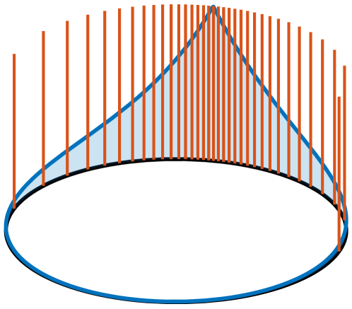
Figure 1: Wrapped Laplace Distribution (blue) on the circular domain (black), with proposed deterministic sampling result for 35 samples (red).

Considered Problem

In this work we consider the problem of deterministic sampling of arbitrary continuous densities on the circular domain with an arbitrary number of samples.

State-of-the-art

The minimalistic and popular deterministic sampling method of normal densities in the Euclidean domain is the basis of the UKF julier1997new ; julier02 . The efficient concept of the UKF has successfully been transferred to the circular domain ACC13_Kurz ; ACC14_Kurz , however inheriting equivalent limitations (only three samples, specific types of densities). Using higher order moments, the number of samples can be increased to five AES16_Kurz and multiples of five with superposition techniques JAIF16_Kurz . For specific densities, sampling based on the CDF has been proposed JAIF16_Kurz but is not invariant w.r.t. interval choice.

Weighted samples in an equidistant grid are very well suited for the circular domain MFI16_Kurz , the sphere IFAC20_Pfaff , and the torus MFI20_Pfaff but expensive to extend to a high number of dimensions. UKF-like sampling methods by contrast are applied to higher-dimensional directional estimation for orientations on the hypersphere TAC16_Gilitschenski ; SPL16_Kurz , for multivariate circular estimation on the torus TAES17_Kurz , and for dual quaternions on special Euclidean groups IFAC20_Li-UPF ; LCSS21_Li , general Lie groups Brossard2017 , or arbitrary Riemannian manifolds Hauberg2013 ; Menegaz2019 – all without exponential increase of computational cost.

How can we make deterministic sampling more flexible, i.e., provide more samples than UKF-like schemes, but avoid Cartesian products? One way to achieve this is based on the LCD and a modified Cramér-von Mises distance. The LCD transforms any density (either continuous or DM) to a continuous representation via kernel convolution. The modified Cramér-von Mises distance is basically an $L^{2}$ norm of the difference of densities Izenman1991 but additionally averages over all kernel widths. LCD and modified Cramér-von Mises distance together yield a distance measure between continuous and DM densities in any combination MFI08_Hanebeck-LCD , which has been successfully applied in the Euclidean domain AT15_Hanebeck , especially for Gaussian densities JAIF14_Steinbring-S2KF ; MFI20_Frisch .

Early adaptions to directional estimation applied the LCD in the Euclidean tangent space of the density’s mean, placing samples on the coordinate axes only ECC19_Li or distributing them in the entire tangent space Fusion19_Li . Direct application of the LCD on non-Euclidean manifolds has been performed for sample reduction (DM to DM comparison) on the sphere IFAC20_Frisch and for dual quaternion sample reduction in the special Euclidean group SE(2) FUSION20_Li . Unfortunately, this method cannot easily be applied to arbitrary density functions and manifolds, because the involved integrals often do not exist in closed form.

For the special case of the von Mises-Fisher density there is also a very efficient deterministic sampling method that places samples on an arbitrary number of “beams” in a star-like arrangement MFI20_Li . It is very fast and more flexible than UKF-like, but the star-like arrangement doesn’t always cover the state space homogeneously and purely according to the density function.

Contribution

In this paper, we present a method to optimally approximate a continuous angular density function ${\tensor*[^{\operatorfont{C\!}}]{f}{}}({\underline{x}})$ on the circular domain with a DMD ${\tensor*[^{\operatorfont{DM\!}}]{f}{}}({\underline{x}})$ with an arbitrary number of samples.

2 Overview

Key Idea

We propose to extend the PCD from the Euclidean space $\mathbb{R}^{d}$ CISS20_Hanebeck to the circular domain $S^{1}$ and use it for deterministic sampling. By projecting to one-dimensional marginal distributions, we reduce multivariate problems to a set of univariate ones. In the univariate setting, cumulative distributions are uniquely defined and can easily be approximated even for arbitrary density functions.

In other words, we match a continuous density with a DMD in the Radon domain. To optimally capture and transfer all of the density’s details, it is important to include many different projections, which we implement in an iterative manner.

Problem Formulation

${\tensor*[^{\operatorfont{C\!}}]{f}{}}({\underline{x}}),\;{\underline{x}}\in S^{1}$ is an arbitrary continuous density function on the circle, considered as reference density here. The goal is to obtain a DMD

$${\tensor*[^{\operatorfont{DM\!}}]{f}{}}({\underline{x}}) =\frac{1}{L}\sum_{i=1}^{L}\delta({\underline{x}}-\hat{\underline{x}}_{i})$$ (1)

with sample locations $\hat{\underline{x}}_{i}\in S^{1}\,,\;\,i\in\left\{1,2,\ldots,L\right\}$. This DMD should optimally approximate the given continuous reference density, limited in accuracy only by the allowed number of samples $L$. Required inputs are

• the number $L$ of wanted samples,

• a numerical function handle of a continuous angular reference density function ${\tensor*[^{\operatorfont{C\!}}]{f}{}}({\underline{x}}),\;{\underline{x}}\in S^{1}$.

Obtained outputs are the sample locations $\hat{\underline{x}}_{i}\in S^{1}$.

3 Projection of the Circular Domain

Projection along a certain direction ${\underline{u}}\in S^{1}$ allows to compare one-dimensional PDF $f(r|{\underline{u}})$ at a time. CDF $F(r|{\underline{u}})$ are uniquely defined in one dimension and can also be easily calculated from the PDF via the trapezoidal rule with proposal samples (if no closed-form solution is available). Furthermore it is easy to compare two one-dimensional CDF.

The following two types of projections $f(r|{\underline{u}})$ of circular densities $f({\underline{x}})$, exponential map and orthographic projection, appear to be equally convenient for our purpose.

3.1 Exponential Map

Consider the circular domain as a real interval of length $2\pi$ by cutting the unit circle open at an arbitrary position ${\underline{u}}\in S^{1}$

$$f(r|{\underline{u}}) =\begin{cases}f\!\left(\begin{bmatrix}\cos(r-\angle{\underline{u}})\\ \sin(r-\angle{\underline{u}})\end{bmatrix}\right)\;,&0\leq r\leq 2\pi\;,\\ 0\;,&\text{otherwise}\;,\end{cases}$$ (2)

where $\angle{\underline{u}}={\operatorfont{atan2}}({\underline{u}}^{(2)},\,{\underline{u}}^{(1)})$ is an angular representation of ${\underline{u}}$.

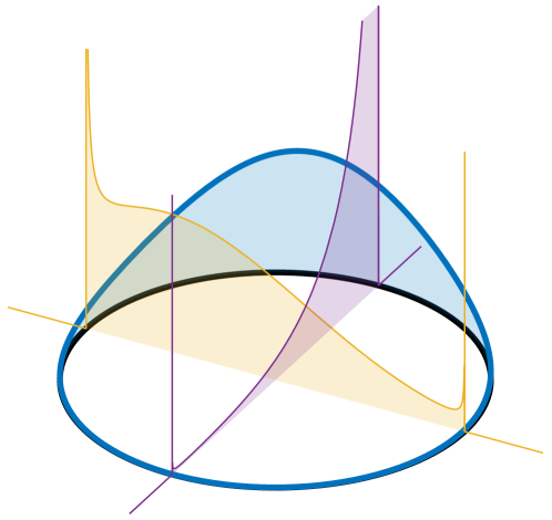
Figure 2: Continuous density function (blue) and two orthographic projections or marginals (yellow, purple), see (7).

3.2 Orthographic Projection

Consider the Euclidean embedding of the circular manifold $S^{1}$ in $\mathbb{R}^{2}$. We then perform a linear projection using the direction vector ${\underline{u}}$

$${\boldsymbol{r}} ={\underline{u}}^{\top}\underline{\boldsymbol{x}}\enspace,$$ (3)

yielding a univariate random variable ${\boldsymbol{r}}$. In terms of densities, we calculate the marginal distribution along ${\underline{u}}$

$$f(r|{\underline{u}}) =\int_{S^{1}}f({\underline{x}})\,\delta(r-{\underline{u}}^{\top}{\underline{x}}){\,\operatorfont{d}}{\underline{x}}\quad\left|\;\alpha\right.=\angle{\underline{x}}$$ (4)

$$=\int\limits_{\alpha=0}^{2\pi}\!\!f\!\left(\begin{bmatrix}\cos(\alpha)\\ \sin(\alpha)\end{bmatrix}\right)\delta\!\left(\!r-\!\begin{bmatrix}\cos(\angle{\underline{u}})\\ \sin(\angle{\underline{u}})\end{bmatrix}^{\!\!\top}\!\!\!\begin{bmatrix}\cos(\alpha)\\ \sin(\alpha)\end{bmatrix}\right)\!\operatorfont{d}\alpha$$ (5)

$$=\int\limits_{\alpha=0}^{2\pi}f\!\left(\begin{bmatrix}\cos(\alpha)\\ \sin(\alpha)\end{bmatrix}\right)\delta\!\left(r-\cos(\alpha-\angle{\underline{u}})\right){\,\operatorfont{d}}\alpha$$ (6)

$$=\begin{cases}\displaystyle\sum_{i=1}^{2}f\!\left(\begin{bmatrix}\cos(\alpha_{i}+\angle{\underline{u}})\\ \sin(\alpha_{i}+\angle{\underline{u}})\end{bmatrix}\right)\!\frac{1}{\left|\sin(\alpha_{i})\right|}\,,&\left|r\right|\leq 1\,,\\ 0\,,&\left|r\right|>1\,,\end{cases}$$ (7)

with

$$\alpha_{i} =\begin{cases}\arccos(r)\,,&i=1,\\ 2\pi-\arccos(r)\;,&i=2\enspace.\end{cases}$$ (8)

See Fig. 2 for a visualization of two orthographic projections.

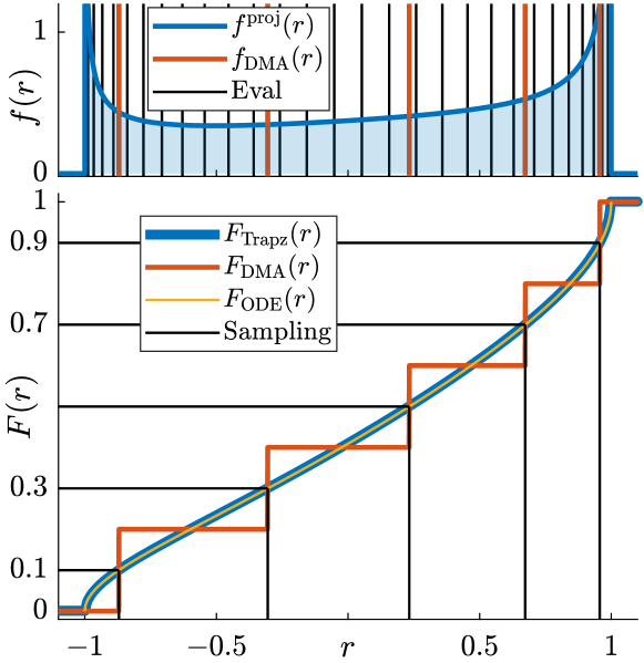
Figure 3: Procedure for deterministic sampling of a projected von Mises-Fisher density, using orthographic projection (7). Upper part: we evaluate $f(r)$ (blue) at the fixed evaluation points $t_{j}^{{\operatorfont{h}}}$ (black) as well as previous sample locations (red). Lower part: Trapezoidal integration on said evaluation points is performed (blue). Compare the ground truth obtained with a numerical ODE solver (yellow). Then, one-dimensional deterministic sampling is performed (black), yielding an approximating DM distribution function (red). See also Alg. 1 for a more detailed description.

4 Implementation

With a suitable projection at hand, we can now start approximating the continuous density. It is well known that samples of any one-dimensional density, like our projected PDF, can easily be drawn when the inverse of the CDF is available. Therefore, we seek to obtain the following intermediate results one by one in the course of this section:

• reference PDF ${\tensor*[^{\operatorfont{C\!}}]{f}{}}({\underline{x}})$ (is given),

• projected PDF ${\tensor*[^{\operatorfont{C\!}}]{f}{}}(r|{\underline{u}})$,

• projected CDF ${\tensor*[^{\operatorfont{C\!}}]{F}{}}(r|{\underline{u}})$,

• inverse CDF ${\tensor*[^{\operatorfont{C\!}}]{F}{}}^{-1}(p|{\underline{u}})$,

• sample locations $r_{i}$,

• sample updates $\Delta{\underline{x}}_{i}$.

The procedure will then be repeated iteratively for different projections ${\underline{u}}$.

Function

$\left\{\Delta r_{i}\right\}_{i=1}^{L}\leftarrow$ sample1D( $f_{{\boldsymbol{r}}}(\cdot),\;\left\{r_{i}\right\}_{i=1}^{L}\;$ )

Input: $f_{{\boldsymbol{r}}}(\cdot)$: continuous reference density in one dimension,
$\left\{r_{i}\right\}_{i=1}^{L}$: current sample approximation

Output: $\left\{\Delta r_{i}\right\}_{i=1}^{L}$: proposed step for each sample, to improve similarity to $f_{{\boldsymbol{r}}}(\cdot)$

$\left\{t_{i}^{{\operatorfont{h}}}\right\}_{i=1}^{L^{{\operatorfont{h}}}}$

  // Fixed evaluation points

$\left\{t_{j}\right\}_{j=1}^{L^{{\operatorfont{e}}}=L^{{\operatorfont{h}}}+L}\leftarrow\left\{t_{i}^{{\operatorfont{h}}}\right\}_{i=1}^{L^{{\operatorfont{h}}}}\;\cup\;\left\{r_{i}\right\}_{i=1}^{L}$

$\left\{F_{j}\right\}_{j=1}^{L^{{\operatorfont{e}}}}\leftarrow$ cumtrapz( $\left\{t_{j}\right\}_{j=1}^{L^{{\operatorfont{e}}}},\;\left\{f_{{\boldsymbol{r}}}(t_{j})\right\}_{j=1}^{L^{{\operatorfont{e}}}}\;$ )

$\left\{F_{j}\right\}_{j=1}^{L^{{\operatorfont{e}}}}\leftarrow\left\{F_{j}+\frac{1-F_{L^{{\operatorfont{e}}}}}{2}\right\}_{j=1}^{L^{{\operatorfont{e}}}}$

  // Centering

for  $i\leftarrow 1$ to $L$  do

       $F^{{\operatorfont{det}}}\leftarrow\frac{2i-1}{2L}$

        // Deterministic sampling

       $\left(j^{{\operatorfont{L}}},j^{{\operatorfont{R}}}\right)\leftarrow$ adjacent( $F^{{\operatorfont{det}}},\;\left\{F_{j}\right\}_{j=1}^{L^{{\operatorfont{e}}}}\;$)

       // Quadratic interpolation

       $m\leftarrow\frac{f_{j^{{\operatorfont{R}}}}-f_{j^{{\operatorfont{L}}}}}{t_{j^{{\operatorfont{R}}}}-t_{j^{{\operatorfont{L}}}}}$

       $(a,b,c)\leftarrow F_{j^{{\operatorfont{L}}}}+\int_{t_{j^{{\operatorfont{L}}}}}^{x}m\cdot\left(x-t_{j^{{\operatorfont{L}}}}\right){\,\operatorfont{d}}x\overset{!}{=}F^{{\operatorfont{det}}}$

       $(x_{1}^{{\operatorfont{quad}}},x_{2}^{{\operatorfont{quad}}})\leftarrow$ roots( $a,b,c\;$ )

       // Linear interpolation

       $x^{{\operatorfont{lin}}}\leftarrow\frac{F^{{\operatorfont{det}}}-F_{j^{{\operatorfont{L}}}}}{m}+t_{j^{{\operatorfont{L}}}}$

       // Updated sample location

       $r_{i}^{{\operatorfont{e}}}\leftarrow$ select_best( $x_{1}^{{\operatorfont{quad}}},\;x_{2}^{{\operatorfont{quad}}},\;x^{{\operatorfont{lin}}}\;$ )

      

end for

// Assign $r_{i}$ and $r_{i}^{{\operatorfont{e}}}$

$\left(\left\{r_{i}^{{\operatorfont{sort}}}\right\}_{i=1}^{L},\;\left\{j_{i}\right\}_{i=1}^{L}\right)\leftarrow$ sort( $\left\{r_{i}\right\}_{i=1}^{L}\;$ )

for  $i\leftarrow 1$ to $L$  do

       $\Delta r_{j_{i}}\leftarrow r_{i}^{{\operatorfont{e}}}-r_{i}^{{\operatorfont{sort}}}$

        // Sample step

      

end for

Algorithm 1 Calculate sample steps that make a DMD approximate a continuous density by matching the cumulatives, in the univariate (projected) setting.

4.1 Composite Trapezoidal Integration

The projected PDF ${\tensor*[^{\operatorfont{C\!}}]{f}{}}(r|{\underline{u}})$ is available in closed form by inserting the given ${\tensor*[^{\operatorfont{C\!}}]{f}{}}({\underline{x}})$ into (2) or (7). Since we are permitting arbitrary density functions, a closed-form representation of the according CDF

$${\tensor*[^{\operatorfont{C\!}}]{F}{}}(r|{\underline{u}}) =\int_{t=-\infty}^{r}f(t|{\underline{u}}){\,\operatorfont{d}}t$$ (9)

is not possible in general. However, we know that the integrand $f(r|{\underline{u}})$ has limited support, i.e., $r\in[0,2\pi]$ for the exponential map projection (2), and $r\in[-1,1]$ for the orthographic projection (7). To obtain an approximation of $F(r|{\underline{u}})$, we apply the composite trapezoidal rule with an adaptive set of function evaluation points $t_{j}$.

A fixed set of homogeneous function evaluation points $t_{j}^{\operatorfont{h}}$ inside the support interval is always used to ensure a good general approximation of the CDF’s global shape. Additionally, in order to maintain proper accuracy of the numerical integral even in the case of very localized PDF with small extent, the projected samples $r_{i}^{\operatorfont{p}}$ in the currently assumed approximating density ${\tensor*[^{\operatorfont{DM\!}}]{f}{}}(r|{\underline{u}})$ are always included into the set of function evaluation points.

Summarizing, after composite trapezoidal integration of ${\tensor*[^{\operatorfont{C\!}}]{f}{}}(r|{\underline{u}})$ with said evaluation points, we now have a piecewise linear representation of the projected reference CDF, ${\tensor*[^{\operatorfont{C\!}}]{F}{}}(r|{\underline{u}})$.

Function $\left\{\hat{\underline{x}}_{i}\right\}_{i=1}^{L}\leftarrow$ sampleS1( $f_{\underline{\boldsymbol{x}}}(\cdot),\;L\;$)

Input: $f_{\underline{\boldsymbol{x}}}(\cdot)$: continuous circular density, ${\underline{x}}\in S^{2}$,
$L$: number of wanted samples

Output: $\left\{\hat{\underline{x}}_{i}\right\}_{i=1}^{L}$: deterministic samples on the circle that approximate $f_{\underline{\boldsymbol{x}}}(\cdot)$

$N\leftarrow 2$

  // Projections per iteration

// High quality for visualization

$M\leftarrow 200$

  // Number of iterations

$\lambda_{0}\leftarrow 0.99$

  // Update step decrease factor

// Initialization

$\lambda\leftarrow 1$

$\left\{\hat{\underline{x}}_{i}\right\}_{i=1}^{L}\leftarrow$ rand( $L,\;S^{2}\,$ )

for  $m\leftarrow 1$ to $M$  do

       $\varphi_{0}\leftarrow$ rand( $1,\;S^{2}\,$ )

       $\left\{\Delta\hat{\underline{x}}_{i}\right\}_{i=1}^{L}\leftarrow\underline{0}$

       for  $n\leftarrow 1$ to $N$  do

             // Symmetric projections

             $\varphi\leftarrow\pi\cdot(n-1)/N+\varphi_{0}$

             ${\underline{u}}\leftarrow\begin{bmatrix}\cos(\varphi)\\ \sin(\varphi)\end{bmatrix}$

             // Project the samples $\hat{\underline{x}}_{i}\rightarrow r_{i}$

             $\left\{r_{i}\right\}_{i=1}^{L}\leftarrow\left\{{\underline{u}}^{\top}\hat{\underline{x}}_{i}\right\}_{i=1}^{L}$

             // Project the density $f_{\underline{\boldsymbol{x}}}(\cdot)\rightarrow f_{{\boldsymbol{r}}}(\cdot|{\underline{u}})$

             // according to Sec. 3

             $f_{{\boldsymbol{r}}}(\cdot)\leftarrow$ project( $f_{\underline{\boldsymbol{x}}}(\cdot),\;{\underline{u}}\;$ )

             // Get projected sample updates

             // using Alg. 1

             $\left\{\Delta r_{i}\right\}_{i=1}^{L}\leftarrow$ sample1D( $f_{{\boldsymbol{r}}}(\cdot),\;\left\{r_{i}\right\}_{i=1}^{L}\;$ )

             // Get sample updates in $\mathbb{R}^{2}$

             $\left\{\Delta{\underline{x}}_{i}\right\}_{i=1}^{L}\leftarrow\{$ backproject( $\Delta r_{i}\;$ ) $\}_{i=1}^{L}$

             $\left\{\Delta\hat{\underline{x}}_{i}\right\}_{i=1}^{L}\leftarrow\left\{\Delta\hat{\underline{x}}_{i}+\Delta{\underline{x}}_{i}\right\}_{i=1}^{L}$

            

       end for

      $\lambda\leftarrow\lambda\cdot\lambda_{0}$

       for  $i\leftarrow 1$ to $L$  do

             // Perform sample update

             $\hat{\underline{x}}_{i}\leftarrow\hat{\underline{x}}_{i}+\lambda\,\Delta\hat{\underline{x}}_{i}/N$

             // Restrict to $S^{2}$

             $\varphi_{i}\leftarrow$ atan2( $\hat{\underline{x}}_{i}^{(2)},\;\hat{\underline{x}}_{i}^{(1)}\;$ )

             $\hat{\underline{x}}_{i}\leftarrow\begin{bmatrix}\cos(\varphi_{i})\\ \sin(\varphi_{i})\end{bmatrix}$

       end for

      

end for

Algorithm 2 PCD-based deterministic sampling of conditional circular densities.

4.2 Deterministic Sampling

We draw deterministic samples $p_{i}$ that are uniformly distributed in $[0,1]\,$,

$$p_{i} =\frac{2i-1}{2L}\;, i \in\left\{1,2,\ldots,L\right\}\;,$$ (10)

and propagate them through the inverse CDF to obtain deterministic samples $r_{i}$ of ${\tensor*[^{\operatorfont{C\!}}]{f}{}}(r|{\underline{u}})$

$$r_{i} ={\tensor*[^{\operatorfont{C\!}}]{F}{}}^{-1}(p_{i}|{\underline{u}})\;, i \in\left\{1,2,\ldots,L\right\}\;.$$ (11)

Under the assumptions that have been made with the trapezoidal rule, our representation of ${\tensor*[^{\operatorfont{C\!}}]{f}{}}(r|{\underline{u}})$ is piecewise linear, and thus ${\tensor*[^{\operatorfont{C\!}}]{F}{}}(r|{\underline{u}})$ is a piecewise quadratic. Therefore, evaluation of ${\tensor*[^{\operatorfont{C\!}}]{F}{}}^{-1}(p_{i}|{\underline{u}})$ for any $p_{i}$ to obtain $r_{i}$ involves two things. First, a search for the relevant interval, i.e., an adjacent pair $(t_{{\operatorfont{L}}},t_{{\operatorfont{R}}})$ from the trapezoidal function evaluation points $t_{i}$ such that ${\tensor*[^{\operatorfont{C\!}}]{F}{}}(t_{{\operatorfont{L}}}|{\underline{u}})\leq p_{i}<{\tensor*[^{\operatorfont{C\!}}]{F}{}}(t_{{\operatorfont{R}}}|{\underline{u}})$. Second, the quadratic (or sometimes linear) function that represents the CDF in this segment has to be inverted, what is easily done in closed form.

Of course, if a closed-form representation of the projected CDF or its inverse is available, we can use that directly for sampling, with no need for trapezoidal integration. For example, a fast approximation of the von Mises-Fisher density’s cumulative (in conjunction with the exponential map) is available in closed form Hill1977 .

At this point we have the deterministic sample locations $r_{i}$ in the projected space that is defined by the projection direction ${\underline{u}}$.

Compare Fig. 3 for a visualization of CDF-based sampling in the projected space.

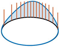
(a) von Mises

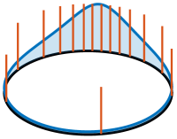
(b) wrapped Cauchy

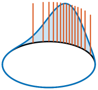
(c) wrapped normal

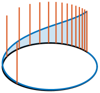
(d) wrapped exponential

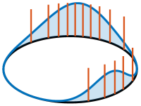
(e) von Mises mixture

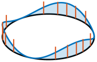
(f) custom distribution, sinusoidal

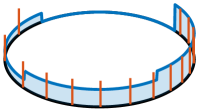
(g) piecewise constant

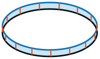
(h) uniform

Figure 4: Illustration of various circular distributions and deterministic samples obtained with the proposed method. Continuous probability density function (blue) on the angular domain $S^{1}$ (black), with sampling results (red). For better visualization, the length of the red lines representing the unweighted samples has been set to the maximum density function value (mode) instead of the sample weight $1/L$.

4.3 Sample Update

The projected sample locations $r_{i}$ now have to be backprojected to the original domain $S^{1}$. We typically use updates from several symmetrically arranged projections simultaneously.

The projected samples generated as described in Sec. 4.2 are not naturally associated with the existing samples from previous iterations. Thus, we have to find an appropriate association first. Projection also helps us here: in the one-dimensional case, the association that minimizes the global distance of associated point pairs can simply be obtained by element-wise comparison of the sorted sets. The according global distance is also called Wasserstein distance.

Refer to Alg. 1 for a pseudocode representation of the procedure described in Sec. 4 up to here.

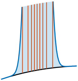
(a) Fixed

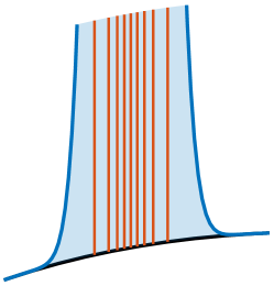
(b) Adaptive

Figure 5: Deterministic circular sampling using (a) only a fixed set of 30 evaluation points $t_{j}^{{\operatorfont{h}}}$ versus (b) the 30 fixed points plus the previous samples, for better numerical integration. The difference for this quite “narrow” von Mises-Fisher distribution ($\kappa=500$) is notable.

4.4 Multiple Projections

To equally consider all dimensions, we propose to use a symmetric set of $N$ projections in each iteration step. For $N=2$ projections per iteration, we choose projections that are orthogonal ($90\text{\,}\mathrm{\SIUnitSymbolDegree}\text{/}$ between them) but with random orientation, see Fig. 2 for an example. The individual sample updates from each projection are averaged, thus yielding the total update $\Delta\hat{\underline{x}}_{i}$ of the current iteration step.

4.5 Iterative Update

The procedure is repeated until the arrangement of the samples obtains an acceptable quality. In order to asymptotically reach a stationary state, we propose to multiply sample updates with an exponentially decreasing factor $\lambda$. This accounts for the fact that more and more information (from more projections) is already present in the sample locations, and the amount of extra information provided by every additional iteration decreases.

Refer to Alg. 2 for a more detailed presentation regarding the iterative sample update scheme.

5 Evaluation

The flexibility of the proposed method is demonstrated by showing obtained deterministic samples form various different density functions, see Fig. 4.

Our adaptive choice of evaluation points for numerical integration allows for an accurate approximation even for “narrow” densities, where fixed evaluation points alone would not be sufficient. See Fig. 5 for an example.

6 Conclusions

We present a method to generate any number of deterministic samples for any continuous density function on the circle.

It does not require gradient-based numerical optimization like LCD-based methods. Instead, we use the trapezoidal rule with adaptive support points on a given interval in an iterative method. Furthermore, the distance measure is simple and undisputable: Matching the cumulatives is always an adequate solution for univariate densities. No parameters or weighting functions have to be chosen. With the help of the PCD, we can apply the same elementary method (matching one-dimensional cumulatives) to higher dimensions.

In the future, we will extend this method to higher-dimensional geometries such as the hypersphere and the torus. While calculating the projected density was easy on the circle, it will be more difficult in higher dimensions. We will look for closed-form solutions that work for specific types of densities. Furthermore, numerical integration techniques with an adaptive choice of evaluation points will be pursued and also pure sample reduction techniques, where no integration is necessary. Presumably, orthographic projection is a good choice for hyperspherical higher-dimensional extensions of the circle, and the exponential map for the Cartesian product of circles, i.e., toroidal manifolds.

References

- (1) W. K. Hastings, “Monte Carlo sampling methods using Markov chains and their applications,” Biometrika, vol. 57, no. 1, pp. 97–109, 04 1970. [Online]. Available: https://doi.org/10.1093/biomet/57.1.97
- (2) G. Kurz and U. D. Hanebeck, “Stochastic Sampling of the Hyperspherical von Mises–Fisher Distribution Without Rejection Methods,” in Proceedings of the IEEE ISIF Workshop on Sensor Data Fusion: Trends, Solutions, Applications (SDF 2015), Bonn, Germany, Oct. 2015.
- (3) G. Kurz, M. Dolgov, and U. D. Hanebeck, “Nonlinear Stochastic Model Predictive Control in the Circular Domain,” in Proceedings of the 2015 American Control Conference (ACC 2015), Chicago, Illinois, USA, Jul. 2015.
- (4) G. Kurz and U. D. Hanebeck, “Heart Phase Estimation Using Directional Statistics for Robotic Beating Heart Surgery,” in Proceedings of the 18th International Conference on Information Fusion (Fusion 2015), Washington D.C., USA, Jul. 2015.
- (5) K. Li, D. Frisch, S. Radtke, B. Noack, and U. D. Hanebeck, “Wavefront Orientation Estimation Based on Progressive Bingham Filtering,” in Proceedings of the IEEE ISIF Workshop on Sensor Data Fusion: Trends, Solutions, Applications (SDF 2018), Oct. 2018.
- (6) S. Bultmann, K. Li, and U. D. Hanebeck, “Stereo Visual SLAM Based on Unscented Dual Quaternion Filtering,” in Proceedings of the 22nd International Conference on Information Fusion (Fusion 2019), Ottawa, Canada, Jul. 2019.
- (7) S. J. Julier and J. K. Uhlmann, “New Extension of the Kalman Filter to Nonlinear Systems,” in Signal Processing, Sensor Fusion, and Target Recognition VI, vol. 3068. International Society for Optics and Photonics, Jul. 1997, pp. 182–193.
- (8) S. J. Julier, “The Scaled Unscented Transformation,” in Proceedings of the 2002 American Control Conference (IEEE Cat. No.CH37301), vol. 6, May 2002, pp. 4555–4559 vol.6.
- (9) G. Kurz, I. Gilitschenski, and U. D. Hanebeck, “Recursive Nonlinear Filtering for Angular Data Based on Circular Distributions,” in Proceedings of the 2013 American Control Conference (ACC 2013), Washington D.C., USA, Jun. 2013.
- (10) ——, “Nonlinear Measurement Update for Estimation of Angular Systems Based on Circular Distributions,” in Proceedings of the 2014 American Control Conference (ACC 2014), Portland, Oregon, USA, Jun. 2014.
- (11) ——, “Recursive Bayesian Filtering in Circular State Spaces,” IEEE Aerospace and Electronic Systems Magazine, vol. 31, no. 3, pp. 70–87, Mar. 2016.
- (12) G. Kurz, I. Gilitschenski, R. Y. Siegwart, and U. D. Hanebeck, “Methods for Deterministic Approximation of Circular Densities,” Journal of Advances in Information Fusion, vol. 11, no. 2, pp. 138–156, Dec. 2016. [Online]. Available: http://confcats_isif.s3.amazonaws.com/web-files/journals/entries/JAIF_Vol11_2_3.pdf
- (13) G. Kurz, F. Pfaff, and U. D. Hanebeck, “Discrete Recursive Bayesian Filtering on Intervals and the Unit Circle,” in Proceedings of the 2016 IEEE International Conference on Multisensor Fusion and Integration for Intelligent Systems (MFI 2016), Baden-Baden, Germany, Sep. 2016.
- (14) F. Pfaff, K. Li, and U. D. Hanebeck, “The Spherical Grid Filter for Nonlinear Estimation on the Unit Sphere,” in Proceedings of the 1st Virtual IFAC World Congress (IFAC-V 2020), Jul. 2020.
- (15) ——, “Estimating Correlated Angles Using the Hypertoroidal Grid Filter,” in Proceedings of the 2020 IEEE International Conference on Multisensor Fusion and Integration for Intelligent Systems (MFI 2020), Virtual, Sep. 2020.
- (16) I. Gilitschenski, G. Kurz, S. J. Julier, and U. D. Hanebeck, “Unscented Orientation Estimation Based on the Bingham Distribution,” IEEE Transactions on Automatic Control, vol. 61, no. 1, pp. 172–177, Jan. 2016.
- (17) G. Kurz, I. Gilitschenski, and U. D. Hanebeck, “Unscented von Mises–Fisher Filtering,” IEEE Signal Processing Letters, vol. 23, no. 4, pp. 463–467, Apr. 2016.
- (18) G. Kurz and U. D. Hanebeck, “Deterministic Sampling on the Torus for Bivariate Circular Estimation,” IEEE Transactions on Aerospace and Electronic Systems, vol. 53, no. 1, pp. 530–534, Feb. 2017.
- (19) K. Li, F. Pfaff, and U. D. Hanebeck, “Hyperspherical Unscented Particle Filter for Nonlinear Orientation Estimation,” in Proceedings of the 1st Virtual IFAC World Congress (IFAC-V 2020), Jul. 2020.
- (20) ——, “Unscented Dual Quaternion Particle Filter for SE(3) Estimation,” IEEE Control Systems Letters, vol. 5, no. 2, pp. 647–652, Apr. 2021. [Online]. Available: https://doi.org/10.1109/LCSYS.2020.3005066
- (21) M. Brossard, S. Bonnabel, and J. Condomines, “Unscented Kalman Filtering on Lie Groups,” in 2017 IEEE/RSJ International Conference on Intelligent Robots and Systems (IROS), 2017, pp. 2485–2491.
- (22) S. Hauberg, F. Lauze, and K. S. Pedersen, “Unscented Kalman Filtering on Riemannian Manifolds,” Journal of Mathematical Imaging and Vision, vol. 46, no. 1, pp. 103–120, May 2013. [Online]. Available: https://doi.org/10.1007/s10851-012-0372-9
- (23) H. M. T. Menegaz, J. Y. Ishihara, and H. T. M. Kussaba, “Unscented Kalman Filters for Riemannian State-Space Systems,” IEEE Transactions on Automatic Control, vol. 64, no. 4, pp. 1487–1502, 2019.
- (24) A. J. Izenman, “Recent Developments in Nonparametric Density Estimation,” Journal of the American Statistical Association, vol. 86, no. 413, pp. 205–224, 1991. [Online]. Available: http://www.jstor.org/stable/2289732
- (25) U. D. Hanebeck and V. Klumpp, “Localized Cumulative Distributions and a Multivariate Generalization of the Cramér-von Mises Distance,” in Proceedings of the 2008 IEEE International Conference on Multisensor Fusion and Integration for Intelligent Systems (MFI 2008), Seoul, Republic of Korea, Aug. 2008, pp. 33–39.
- (26) U. D. Hanebeck, “Optimal Reduction of Multivariate Dirac Mixture Densities,” at – Automatisierungstechnik, Oldenbourg Verlag, vol. 63, no. 4, pp. 265–278, Apr. 2015. [Online]. Available: http://dx.doi.org/10.1515/auto-2015-0005
- (27) J. Steinbring and U. D. Hanebeck, “LRKF Revisited: The Smart Sampling Kalman Filter (S2KF),” Journal of Advances in Information Fusion, vol. 9, no. 2, pp. 106–123, Dec. 2014. [Online]. Available: http://confcats_isif.s3.amazonaws.com/web-files/journals/entries/441_1_art_11_17020.pdf
- (28) D. Frisch and U. D. Hanebeck, “Efficient Deterministic Conditional Sampling of Multivariate Gaussian Densities,” in Proceedings of the 2020 IEEE International Conference on Multisensor Fusion and Integration for Intelligent Systems (MFI 2020), Virtual, Sep. 2020.
- (29) K. Li, D. Frisch, B. Noack, and U. D. Hanebeck, “Geometry-Driven Deterministic Sampling for Nonlinear Bingham Filtering,” in Proceedings of the 2019 European Control Conference (ECC 2019), Naples, Italy, Jun. 2019.
- (30) K. Li, F. Pfaff, and U. D. Hanebeck, “Hyperspherical Deterministic Sampling Based on Riemannian Geometry for Improved Nonlinear Bingham Filtering,” in Proceedings of the 22nd International Conference on Information Fusion (Fusion 2019), Ottawa, Canada, Jul. 2019.
- (31) D. Frisch, K. Li, and U. D. Hanebeck, “Optimal Reduction of Dirac Mixture Densities on the 2-Sphere,” in Proceedings of the 1st Virtual IFAC World Congress (IFAC-V 2020), Jul. 2020.
- (32) K. Li, F. Pfaff, and U. D. Hanebeck, “Dual Quaternion Sample Reduction for SE(2) Estimation,” in Proceedings of the 23rd International Conference on Information Fusion (Fusion 2020), Virtual, Jul. 2020.
- (33) ——, “Nonlinear von Mises-Fisher Filtering Based on Isotropic Deterministic Sampling,” in Proceedings of the 2020 IEEE International Conference on Multisensor Fusion and Integration for Intelligent Systems (MFI 2020), Virtual, Sep. 2020.
- (34) U. D. Hanebeck, “Deterministic Sampling of Multivariate Densities based on Projected Cumulative Distributions,” in Proceedings of the 54th Annual Conference on Information Sciences and Systems (CISS 2020), Princeton, New Jersey, USA, Mar. 2020.
- (35) G. W. Hill, “Algorithm 518: Incomplete Bessel Function . The Von Mises Distribution [S14],” ACM Trans. Math. Softw., vol. 3, no. 3, p. 279–284, Sep. 1977. [Online]. Available: https://doi.org/10.1145/355744.355753