Over-approximating reachable tubes of linear time-varying systems

Abstract

We present a method to over-approximate reachable tubes over compact time-intervals, for linear continuous-time, time-varying control systems whose initial states and inputs are subject to compact convex uncertainty. The method uses numerical approximations of transition matrices, is convergent of first order, and assumes the ability to compute with compact convex sets in finite dimension. We also present a variant that applies to the case of zonotopic uncertainties, uses only linear algebraic operations, and yields zonotopic over-approximations. The performance of the latter variant is demonstrated on an example.

I Introduction

Reachable (or attainable) sets and tubes are central concepts in systems and control theory, with myriads of applications. See, e.g. [1, 2, 3, 4, 5, 6, 7] and the references given therein. The efficient computation of accurate approximations of these sets is a challenging problem whose diverse variants have been attracting research attention for decades. In this paper, we focus on over-approximating reachable tubes of linear time-varying control systems of the form

$$\dot{x}(t)=A(t)x(t)+B(t)u(t)$$ (1)

over compact time-intervals $\left[t_{0},t_{f}\right]$, where $A\colon\left[t_{0},t_{f}\right]\to\mathbb{R}^{n\times n}$ and $B\colon\left[t_{0},t_{f}\right]\to\mathbb{R}^{n\times m}$ are time-varying matrices. Both the initial state $x(t_{0})$ and the input signal $u$ are subject to compact convex uncertainty. The problem is mathematically formalized in Section III.

In numerous applications it is critical to formally verify that all solutions of the system ( ‣ I always avoid certain predefined unsafe regions; see, e.g. [4, Sect. 3] and the references given therein. That is, these applications require proof that the reachable tube over the time-interval $\left[t_{0},t_{f}\right]$ (and not only the reachable set at some time $t\in\left[t_{0},t_{f}\right]$) of the system ( ‣ I does not intersect any unsafe region. As tubes cannot, in general, be determined exactly, intersection tests need to rely on over-approximations (and not on mere approximations) in place of the actual tubes. The over-approximations should be as precise as possible to avoid excessive conservatism of the verification, and need to be represented in a form that facilitates to reliably and efficiently verify disjointness from unsafe regions.

One of the earliest techniques of reachability analysis, the hyperplane method, approximates reachable sets by intersections of supporting halfspaces and by convex hulls of the respective support points [8, 1]. More recent techniques rely on a variety of additional classes of sets including, e.g. ellipsoids, hyper-intervals, and zonotopes [5, 7, 9, 10, 11, 12, 13, 14, 15, 16, 17, 6, 18, 19, 20, 21, 22, 23, 24, 25]. As for reachable tubes, the standard approach today is to apply the method proposed in [9] or one of its extensions, e.g. [10, 11, 7, 12, 13], which compute over-approximations in the form of finite unions of zonotopes [9, 10, 7] and of more general convex sets [11, 12, 13]. As a result of such representation, disjointness from a polyhedral (or convex) unsafe region can be verified by solving a linear (or convex) feasibility problem. While the method is particularly efficient and converges, i.e., it is capable of producing arbitrarily precise over-approximations, its application is limited to the time-invariant special case of ( ‣ I. Its extension in [14] additionally allows for uncertain coefficients $A$ and $B$ in ( ‣ I, but does not converge even if $A$ and $B$ are precisely known, in which case ( ‣ I is again required to be time-invariant.

Another prominent class of methods, ellipsoidal techniques [5], solve the more general problem of feedback synthesis for linear time-varying plants with two competing inputs. When applied to the system ( ‣ I, these methods yield a set-valued function $E$ defined on the interval $\left[t_{0},t_{f}\right]$ whose value at any time is a finite intersection of ellipsoids containing the reachable set at that time as a subset. While arbitrarily precise over-approximations are obtained when a sufficient amount of ellipsoids is computed, the approach suffers from two shortcomings. Firstly, the ellipsoids result from numerically solving linear-quadratic optimal control problems derived from ( ‣ I, yet numerical errors incurred in the course of the solution are not taken into account. Hence, mere approximations rather than over-approximations might actually be computed. Secondly, approximations of reachable tubes are obtained only implicitly, as the union over $t\in\left[t_{0},t_{f}\right]$ of $E(t)$, and so they are disjoint from an unsafe region $R$ if and only if the graph of the set-valued map $E$ is disjoint from the set $\left[t_{0},t_{f}\right]\times R$. Verifying the latter condition is a great challenge since the graph of $E$ is not, in general, convex. The issue has so far been resolved only for the time-invariant special case of ( ‣ I; see [15]. Moreover, while ellipsoidal techniques have been generalized to handle nonlinear dynamics, the extensions still suffer from both the aforementioned shortcomings, e.g. [16].

Other approaches use differential inequalities, comparison principles, interval arithmetic, and combinations thereof, and compute interval over-approximations [18, 19, 6, 17, 20]. While these techniques may allow for uncertain coefficients $A$ and $B$ in ( ‣ I [17] or even for nonlinear dynamics [18, 19, 6, 20], they are all conservative, i.e., arbitrarily precise over-approximations of reachable tubes cannot be obtained, and the methods in [18, 19, 6, 17] additionally suffer from both shortcomings mentioned in our discussion of ellipsoidal techniques. Finally, the reachable tube can also be characterized as a sublevel set of the viscosity solution of a partial differential equation called Hamilton-Jacobi-Bellman equation [5]. However, solving the latter numerically is avoided in practice as this would require discretizing the state space and so the computational effort would scale exponentially with the state space dimension.

To conclude, efficient methods to compute arbitrarily precise over-approximations of reachable tubes of the system ( ‣ I, that are additionally represented in a form suitable for formal verification purposes, are currently limited to the time-invariant special case of ( ‣ I. This is in stark contrast to the importance of the general time-varying case of ( ‣ I in several fields of application, e.g. [26].

In Section IV-A of this paper, we present a method that produces over-approximations that are convergent of first order, does not require discretization of either the input or the state space, uses numerical approximations of transition matrices rather than closed-form solutions, and assumes the ability to compute with compact convex sets in finite dimension. A variant that applies to the case of zonotopic uncertainties, uses only linear algebraic operations, and yields zonotopic over-approximations, is subsequently presented in Section IV-B. In Section V, we demonstrate the performance of the latter variant on an example.

II Preliminaries

II-A Notation

Given two sets $A$ and $B$ and a positive integer $p$, $B\setminus A$ and $A\times B$ denotes the relative complement of the set $A$ in the set $B$, and the product of $A$ and $B$, respectively, and $A^{p}=A\times\cdots\times A$ ($p$ factors). $\mathbb{R}$, $\mathbb{R}_{+}$, $\mathbb{Z}$ and $\mathbb{Z}_{+}$ denote the sets of real numbers, non-negative real numbers, integers and non-negative integers, respectively, and $\mathbb{N}=\mathbb{Z}_{+}\setminus\{0\}$. $\left[a,b\right]$, $\left\orbrack a,b\right\clbrack$, $\left[a,b\right\clbrack$, and $\left\orbrack a,b\right]$ denote closed, open and half-open, respectively, intervals with end points $a$ and $b$, e.g. $\left[0,\infty\right\clbrack=\mathbb{R}_{+}$. $\left[a;b\right]$, $\left\orbrack a;b\right\clbrack$, $\left[a;b\right\clbrack$, and $\left\orbrack a;b\right]$ stand for discrete intervals, e.g. $\left[a;b\right]=\left[a,b\right]\cap\mathbb{Z}$, $\left[1;4\right\clbrack=\{1,2,3\}$, and $\left[0;0\right\clbrack=\emptyset$.

Given any map $f\colon A\to B$, the image of a subset $C\subseteq A$ under $f$ is denoted $f(C)$, $f(C)=\left\{f(c)\,\middle|\,c\in C\right\}$. We denote the identity map $X\to X\colon x\mapsto x$ by $\operatorname{id}$, where the domain of definition $X$ will always be clear form the context.

Arithmetic operations involving subsets of a linear space $X$ are defined pointwise, e.g. $\alpha M\mathrel{:=}\left\{\alpha y\,\middle|\,y\in M\right\}$ and the Minkowski sum $M+N\mathrel{:=}\left\{y+z\,\middle|\,y\in M,z\in N\right\}$, if $\alpha\in\mathbb{R}$ and $M,N\subseteq X$. The convex hull of $M$ is denoted $\mathop{\rm conv}\nolimits(M)$. By $\|\cdot\|$ we denote any norm on $X$, $\mathbb{B}\subseteq X$ is the closed unit ball w.r.t. $\|\cdot\|$, and the norm of a non-empty subset $M\subseteq X$ is defined by $\|M\|\mathrel{:=}\sup_{x\in M}\|x\|$. The maximum norm on $\mathbb{R}^{n}$ is denoted $\|\cdot\|_{\infty}$, $\|x\|_{\infty}=\max\left\{|x_{i}|\,\middle|\,i\in\left[1;n\right]\right\}$ for all $x\in\mathbb{R}^{n}$. The Hausdorff distance $d_{H}$ is defined in the Appendix.

We say that a map is of class $C^{k}$ if it is continuous and $k$ times continuously differentiable, $k\in\mathbb{Z}_{+}$. Given a non-empty set $X\subseteq\mathbb{R}^{n}$ and a compact interval $\left[a,b\right]\subseteq\mathbb{R}$, $X^{\left[a,b\right]}$ denotes the set of all measurable maps $\left[a,b\right]\to X$. Integration is always understood in the sense of Lebesgue. Given norms on $\mathbb{R}^{n}$ and $\mathbb{R}^{m}$, the linear space $\mathbb{R}^{n\times m}$ of $n\times m$ matrices is endowed with the usual matrix norm, $\|A\|=\sup_{\|x\|\leq 1}\|Ax\|$ for $A\in\mathbb{R}^{n\times m}$.

We use the asymptotic notation $O(\cdot)$ in the usual way [27]. In particular, let $X\subseteq\mathbb{R}^{n}$, $f\colon F\subseteq\mathbb{R}\times X\to\mathbb{R}_{+}$, $g\colon G\subseteq\mathbb{R}\to\mathbb{R}_{+}$, $H\colon F\times\mathbb{R}_{+}\to\mathbb{R}_{+}$ and $a\in\mathbb{R}$ be such that $a=\lim_{i\to\infty}s_{i}$ for some sequence $(s_{i},x_{i})_{i\in\mathbb{N}}$ in $F$, and suppose that $s\in G$ whenever $(s,x)\in F$. Then $f(s,x)\leq H(s,x,O(g(s)))$ as $s\to a$, uniformly in $x$, if there exist $k\colon G\to\mathbb{R}_{+}$ and a neighborhood $U\subseteq\mathbb{R}$ of $a$ such that $k(s)=O(g(s))$ as $s\to a$ and $f(s,x)\leq H(s,x,k(s))$ whenever $(s,x)\in F\cap(U\times X)$, and similarly for $a\in\{\infty,-\infty\}$.

II-B Linear Time-Varying Control Systems

Given $u\colon\left[t_{0},t_{f}\right]\to\mathbb{R}^{m}$, a map $x\colon\left[t_{0},t_{f}\right]\to\mathbb{R}^{n}$ is a solution of the system ( ‣ I (generated by $u$) if $x$ is absolutely continuous and ( ‣ I holds for (Lebesgue) almost every $t\in\left[t_{0},t_{f}\right]$. We shall always assume that $A$ and $B$ are continuous and that $u$ is integrable, which implies both existence and uniqueness of solutions [28]. The general solution of the system ( ‣ I is the map $\varphi$ defined by the requirement that for all $p\in\mathbb{R}^{n}$, $s\in\left[t_{0},t_{f}\right]$ and integrable $u$, $\varphi(\cdot,s,p,u)$ is the unique solution of ( ‣ I defined on $\left[t_{0},t_{f}\right]$ and satisfying $\varphi(s,s,p,u)=p$. The map $\varphi(t,s,\cdot,0)$, which is linear, is called the transition matrix at $(t,s)$ of the system and is denoted by $\phi(t,s)$. The map $\phi\colon\left[t_{0},t_{f}\right]\times\left[t_{0},t_{f}\right]\to\mathbb{R}^{n\times n}$ is of class $C^{1}$, and the identities

$$\varphi(t,s,p,u)=\phi(t,s)p+\int_{s}^{t}\phi(t,\tau)B(\tau)u(\tau)d\tau,$$

$\phi(s,s)=\operatorname{id}$, and $\phi(t,s)\phi(s,T)=\phi(t,T)$ hold for all $s,t,T\in\left[t_{0},t_{f}\right]$, all $p\in\mathbb{R}^{n}$, and all integrable $u$; see, e.g. [28]. Moreover, $D_{1}\phi(t,s)=A(t)\phi(t,s)$ and $D_{2}\phi(s,t)=-\phi(s,t)A(t)$ hold for all $s,t\in\left[t_{0},t_{f}\right]$, where $D_{i}\phi$ denotes the partial derivative of $\phi$ with respect to (w.r.t.) the $i$th argument. If $A$ is additionally of class $C^{k}$, $k\geq 1$, then $\phi$ is of class $C^{k+1}$. Finally, Gronwall’s lemma implies

$$\|\phi(t,s)\|\leq\mathrm{e}^{|t-s|M}\text{\ \ and\ \ }\|\phi(t,s)-\operatorname{id}\|\leq\mathrm{e}^{|t-s|M}-1$$ (2)

for all $s,t\in\left[t_{0},t_{f}\right]$, provided that $\|A(t)\|\leq M$ for all $t\in\left[t_{0},t_{f}\right]$.

II-C Reachable Sets and Tubes

Given non-empty, compact, convex subsets $X_{0}\subseteq\mathbb{R}^{n}$ and $U\subseteq\mathbb{R}^{m}$, and $a,b,t\in\left[t_{0},t_{f}\right]$ satisfying $a\leq b$, the sets

$$\mathcal{R}(t) =\left\{\varphi(t,t_{0},x_{0},u)\,\middle|\,x_{0}\in X_{0},u\in U^{\left[t_{0},t\right]}\right\},$$

$$\mathcal{R}(\left[a,b\right]) =\bigcup_{s\in\left[a,b\right]}\mathcal{R}(s)$$

are the reachable set at time $t$ and the reachable tube over the time interval $\left[a,b\right]$, respectively, of the system ( ‣ I. Both $\mathcal{R}(t)$ and $\mathcal{R}(\left[a,b\right])$ are non-empty and compact, and $\mathcal{R}(t)$ is additionally convex and is conveniently written using a set-valued integral, $\mathcal{R}(t)=\phi(t,t_{0})X_{0}+\int_{t_{0}}^{t}\phi(t,s)B(s)Uds.$ See, e.g. [29]. Moreover, the well-known semi-group property of reachable sets [30] yields the identity

$$\mathcal{R}(b)=\phi(b,a)\mathcal{R}(a)+\int_{a}^{b}\phi(b,s)B(s)Uds.$$ (3)

III Problem Statement

We consider the system ( ‣ I, where both the initial state $x(t_{0})\in X_{0}$ and the input $u(t)\in U$ are subject to uncertainty, represented by the set $X_{0}$ and $U$, respectively. We assume the following.

1. $n\in\mathbb{N}$, $t_{0},t_{f}\in\mathbb{R}$ and $t_{0}<t_{f}$.

2. $X_{0}\subseteq\mathbb{R}^{n}$ and $U\subseteq\mathbb{R}^{m}$ are non-empty, compact, and convex.

3. $A$ and $B$ are of class $C^{1}$, and $\|A(t)\|\leq M_{A}$, $\|\dot{A}(t)\|\leq M_{\dot{A}}$, $\|B(t)\|\leq M_{B}$, and $\|\dot{B}(t)\|\leq M_{\dot{B}}$ for all $t\in\left[t_{0},t_{f}\right]$, where $M_{A},M_{\dot{A}},M_{B},M_{\dot{B}}\in\mathbb{R}$ and $M_{A}>0$. Here, $\dot{A}$ denotes the derivative of the map $A\colon\left[t_{0},t_{f}\right]\to\mathbb{R}^{n\times n}$, and similarly for $\dot{B}$.

4. Denote $D=\left\{(t,s)\in\left[t_{0},t_{f}\right]\times\left[t_{0},t_{f}\right]\,\middle|\,t\geq s\right\}$. Then

   $$\|\phi(t,s)-\widetilde{\phi}(t,s)\| \leq\theta(t-s)\text{ for all $(t,s)\in D$},$$ (4)

   $$\theta(h) =O(h^{2})\text{ as $h\to 0$},$$ (5)

   where $\widetilde{\phi}\colon D\to\mathbb{R}^{n\times n}$ approximates the transition matrix $\phi$ of ( ‣ I and $\theta\colon\mathbb{R}_{+}\to\mathbb{R}_{+}$ is monotonically increasing.

We note that ($H_{4}$) is the requirement that the approximation $\widetilde{\phi}$ of $\phi$ has consistency order $1$ [31, Def. 4.7]. Under assumptions ($H_{1}$)-($H_{3}$), this requirement is satisfied by the vast majority of numerical methods to solve initial value problems. See, e.g. [31, Example 4.8], as well as Lemma .4 in the Appendix.

The problem data $t_{0}$, $t_{f}$, $A$, $B$, $X_{0}$ and $U$ are fixed throughout the paper, and so are the constants $M_{A}$, $M_{\dot{A}}$, $M_{B}$, and $M_{\dot{B}}$, as well as the functions $\phi$, $\widetilde{\phi}$ and $\theta$ and the set $D$. Throughout the paper, all that data is subject to the standing hypotheses ($H_{1}$)-($H_{4}$).

III.1 Problem.

Devise a convergent method that over-approximates $\mathcal{R}(\left[t_{0},t_{f}\right])$, in the sense that given the problem data and a time discretization parameter $N$, a superset $\widehat{R}_{N}$ of $\mathcal{R}(\left[t_{0},t_{f}\right])$ is obtained, satisfying $\widehat{R}_{N}\to\mathcal{R}(\left[t_{0},t_{f}\right])$ in Hausdorff distance as $N\to\infty$.

IV Proposed method

In order to solve Problem III.1 for any given value of the time discretization parameter $N$, we shall over-approximate reachable sets $\mathcal{R}(t_{i})$ and reachable tubes $\mathcal{R}(\left[t_{i},t_{i+1}\right])$ of the control system ( ‣ I for equidistant points of time $t_{i}\in\left[t_{0},t_{f}\right]$, $i\in\left[0;N\right]$. The approximation will be convergent of first order [31], meaning that the Hausdorff distance between $\mathcal{R}(t_{i})$ and its approximation is of order $O(1/N)$, and similarly for tubes. The respective method of over-approximation, presented in Section IV-A, applies to any uncertainty sets $X_{0}$ and $U$ satisfying Hypothesis ($H_{2}$) and assumes the ability to compute with compact convex sets in finite dimension. Our algorithmic solution subsequently presented in Section IV-B applies to the case of zonotopic uncertainties, uses only linear algebraic operations, and involves an additional approximation step that yields zonotopic over-approximations of reachable tubes retaining first order accuracy.

IV-A Over-approximation of Reachable Sets and Reachable Tubes

We consider the system ( ‣ I under our standing hypotheses ($H_{1}$)-($H_{4}$). Given a time discretization parameter $N\in\mathbb{N}$, we define sequences $(\Omega_{i})_{i\in\left[0;N\right]}$ and $(\Gamma_{i})_{i\in\left[1;N\right]}$ of subsets $\Omega_{i},\Gamma_{i}\subseteq\mathbb{R}^{n}$ by the following requirements for all $i\in\left[1;N\right]$.

$$h =(t_{f}-t_{0})/N\text{\ \ and\ \ }t_{i}=t_{0}+ih,$$ (6a)

$$\Omega_{0} =X_{0},$$ (6b)

$$\Omega_{i} =\widetilde{\phi}(t_{i},t_{i-1})\Omega_{i-1}+hB(t_{i})U+(\alpha_{h}+\theta_{h}\|\Omega_{i-1}\|)\mathbb{B},$$ (6c)

$$\Gamma_{i} =\mathop{\rm conv}\nolimits\left(\Omega_{i-1}\cup\left(\Omega_{i}+(\beta_{h}+\gamma_{h}\|\Omega_{i-1}\|)\mathbb{B}\right)\right).$$ (6d)

Here, $$\|\cdot\| \alpha,\beta,\gamma\colon\mathbb{R}_{+}\to\mathbb{R}_{+}$$ denotes any norm and the maps are defined by

$$r(s) =\exp(sM_{A})-1-sM_{A}, \beta(s) =s^{2}M_{\dot{B}}\|U\|,$$ (6e)

$$\alpha(s) =r(s)\|U\|\frac{M_{\dot{B}}+M_{A}M_{B}}{M_{A}^{2}}, \gamma(s) =r(s)\left(1+\frac{M_{\dot{A}}}{M_{A}^{2}}\right)\negthinspace.$$ (6f)

For convenience, here and in the sequel we often use $\alpha_{h}$ in place of $\alpha(h)$, and similarly for $\beta$, $\gamma$ and $\theta$.

By ( ‣ ( ‣ IV-A, we define an equidistant grid with step size $h$, of points $t_{0}$, …, $t_{N}$, spanning the time interval $\left[t_{0},t_{f}\right]$. The requirements ( ‣ ( ‣ IV-A-( ‣ ( ‣ IV-A iteratively define sets $\Omega_{i}$, which are supposed to approximate the reachable sets $\mathcal{R}(t_{i})$, and in turn, ( ‣ ( ‣ IV-A uses these approximations as well as their inflated versions to define sets $\Gamma_{i}$, which are supposed to approximate reachable tubes $\mathcal{R}(\left[t_{i-1},t_{i}\right])$. As we shall show, due to our careful definition of the maps $\alpha$, $\beta$ and $\gamma$ depending on the time-varying problem data, both $\Omega_{i}$ and $\Gamma_{i}$ actually are over-approximations, with approximation error of order $O(1/N)$.

We now set out to state formally and to prove what we have just described in informal terms. In doing so, we shall use the superscript $N$ to indicate that, e.g. the sequence $(\Omega^{N}_{i})_{i\in\left[0;N\right]}$has been computed by our method ( ‣ IV-A for a specific value of the time discretization parameter, and similarly for $h$, $t_{i}$ and $\Gamma_{i}$.

IV.1 Proposition (Reachable Sets).

For each $N\in\mathbb{N}$, let sequences $(t^{N}_{i})_{i\in\left[0;N\right]}$ and $(\Omega^{N}_{i})_{i\in\left[0;N\right]}$ be defined by ( ‣ ( ‣ IV-A-( ‣ ( ‣ IV-A and ( ‣ ( ‣ IV-A-( ‣ ( ‣ IV-A.
Then $\mathcal{R}(t^{N}_{i})\subseteq\Omega^{N}_{i}$ for all $N\in\mathbb{N}$ and all $i\in\left[0;N\right]$, and $d_{H}(\mathcal{R}(t^{N}_{i}),\Omega^{N}_{i})\leq O(1/N)$ as $N\to\infty$, uniformly w.r.t. $i$.

For our proof, we need the following auxiliary results.

IV.2 Lemma.

We have the estimate $d_{H}(I(a,b),J(a,b))\leq\alpha(b-a)$ whenever $t_{0}\leq a\leq b\leq t_{f}$, where $I(a,b)=\int_{a}^{b}\phi(b,s)B(s)Uds$, $J(a,b)=(b-a)B(b)U$, and $\alpha$ is defined in ( ‣ ( ‣ IV-A.

Proof.

Let $a,b\in\left[t_{0},t_{f}\right]$, $a\leq b$. The assumption ($H_{2}$) on $U$ implies $J(a,b)=\int_{a}^{b}B(b)Uds$, and using Filippov’s Lemma [29], we obtain

$$d_{H}(I(a,b),J(a,b))\leq\|U\|\int_{a}^{b}\|\phi(b,s)B(s)-B(b)\|ds.$$ (7)

Next, using ( ‣ II-B and the identity

$$\phi(b,s)B(s)-B(b)=\int_{b}^{s}\phi(b,z)(\dot{B}(z)-A(z)B(z))dz$$

for all $s\in\left[t_{0},t_{f}\right]$, we see that the integrand in ( ‣ IV-A is bounded by $(M_{\dot{B}}+M_{A}M_{B})(\mathrm{e}^{(b-s)M_{A}}-1)/M_{A}$, which proves the lemma. ∎

IV.3 Lemma.

Let $a\in\mathbb{R}_{+}$, $b\in\mathbb{R}$, $K\colon\mathbb{N}\to\mathbb{N}$, and for each $N\in\mathbb{N}$, let $(x^{N}_{i})_{i\in\left[0;K(N)\right]}$ be a sequence in $\mathbb{R}_{+}$. Suppose that $K(N)=O(N^{a})$, $x^{N}_{0}=O(N^{a+b})$ and $x^{N}_{i}\leq(1+O(N^{-a}))x^{N}_{i-1}+O(N^{b})$ hold as $N\to\infty$, uniformly w.r.t. $i$.
Then $x^{N}_{i}\leq O(N^{a+b})$ as $N\to\infty$, uniformly w.r.t. $i$.

Proof.

By our hypotheses, there exist maps $p,q,r\colon\mathbb{N}\to\mathbb{R}_{+}$ satisfying $p(N)=O(N^{a+b})$, $q(N)=O(N^{-a})$ and $r(N)=O(N^{b})$ as $N\to\infty$, and

$$x^{N}_{0}\leq p(N)\text{\ \ and\ \ }x^{N}_{i}\leq(1+q(N))x^{N}_{i-1}+r(N)$$ (8)

for all sufficiently large $N\in\mathbb{N}$ and all $i\in\left[1;K(N)\right]$. Define $f(N,i)=(1+q(N))^{i}$ for all $N\in\mathbb{N}$ and all $i\in\left[0;K(N)\right]$, to arrive at $f(N,i)\leq\exp(q(N)K(N))$. Then, by our assumptions on $q$ and $K$, the map $f$ is bounded. In view of ( ‣ IV-A and the variation-of-constants formula we conclude that $x^{N}_{i}\leq O(N^{a+b})$ as claimed. ∎

Proof of Proposition IV.1.

For the sake of simplicity, throughout this proof we drop the superscript $N$ from our notation. Let $h$ be defined by ( ‣ ( ‣ IV-A.

The first claim holds for $i=0$ and all $N\in\mathbb{N}$ as $\mathcal{R}(t_{0})=X_{0}=\Omega_{0}$. Assume that $\mathcal{R}(t_{i})\subseteq\Omega_{i}$ holds for some $N\in\mathbb{N}$ and some $i\in\left[0;N\right\clbrack$. Then, using the identity ( ‣ II-C and Lemma IV.2 as well as Lemma .2(v), we obtain $\mathcal{R}(t_{i+1})\subseteq\phi(t_{i+1},t_{i})\Omega_{i}+hB(t_{i+1})U+\alpha(h)\mathbb{B}$. Moreover, $\phi(t_{i+1},t_{i})\Omega_{i}\subseteq\widetilde{\phi}(t_{i+1},t_{i})\Omega_{i}+\theta(h)\|\Omega_{i}\|$ by the estimate ( ‣ ($H_{4}$) and Lemma .2(iii)(v), and so $\mathcal{R}(t_{i+1})\subseteq\Omega_{i+1}$.

To prove the second claim, we use the triangle inequality, assumption ($H_{3}$) and estimates ( ‣ II-B, ( ‣ ($H_{4}$) and ( ‣ ($H_{4}$) to obtain the bound $\|\widetilde{\phi}(t_{i},t_{i-1})\|\leq 1+O(1/N)$ as $N\to\infty$, uniformly w.r.t. $i$. In turn, ( ‣ ($H_{4}$), ( ‣ ( ‣ IV-A, ($H_{2}$) and the fact that $\alpha(s)=O(s^{2})$ as $s\to 0$ together imply $\|\Omega_{i}\|\leq(1+O(1/N))\|\Omega_{i-1}\|+O(1/N)$, and so $\|\Omega_{i}\|\leq O(1)$ as $N\to\infty$, uniformly w.r.t. $i$, by Lemma IV.3. It follows that $\alpha(h)+\theta(h)\|\Omega_{i-1}\|\leq O(1/N^{2})$ and $d_{H}(\widetilde{\phi}(t_{i},t_{i-1})\Omega_{i-1},\phi(t_{i},t_{i-1})\mathcal{R}(t_{i-1}))\leq(1+O(1/N))e_{i-1}+O(1/N^{2})$, where $e_{i}=d_{H}(\mathcal{R}(t_{i}),\Omega_{i})$. Moreover, $d_{H}(hB(t_{i})U,\int_{t_{i-1}}^{t_{i}}\phi(t_{i},s)B(s)Uds)\leq O(1/N^{2})$ by Lemma IV.2, and so $e_{i}\leq(1+O(1/N))e_{i-1}+O(1/N^{2})$ as $N\to\infty$, uniformly w.r.t. $i$. Then $e_{i}\leq O(1/N)$ by Lemma IV.3, as claimed. ∎

The following theorem, and its corollary immediately obtained using Lemma .2(vii), provide a first solution to Problem III.1.

IV.4 Theorem (Reachable Tubes).

For each $N\in\mathbb{N}$, let sequences $(t^{N}_{i})_{i\in\left[0;N\right]}$ and $(\Gamma^{N}_{i})_{i\in\left[1;N\right]}$ be defined by ( ‣ IV-A.
Then $\mathcal{R}(\left[t_{i-1},t_{i}\right])\subseteq\Gamma^{N}_{i}$ for all $N\in\mathbb{N}$ and all $i\in\left[1;N\right]$, and $d_{H}(\mathcal{R}(\left[t_{i-1},t_{i}\right]),\Gamma^{N}_{i})\leq O(1/N)$ as $N\to\infty$, uniformly w.r.t. $i$.

IV.5 Corollary.

Under the hypotheses and in the notation of Theorem IV.4, denote $\widehat{R}_{N}=\cup_{i\in\left[1;N\right]}\Gamma^{N}_{i}$. Then $\mathcal{R}(\left[t_{0},t_{f}\right])\subseteq\widehat{R}_{N}$ for all $N\in\mathbb{N}$, and $d_{H}(\mathcal{R}(\left[t_{0},t_{f}\right]),\widehat{R}_{N})=O(1/N)$ as $N\to\infty$.

Our proof of Theorem IV.4 uses the following auxiliary result.

IV.6 Lemma.

Let $\gamma$ be defined by ( ‣ ( ‣ IV-A, and let $a,b\in\left[t_{0},t_{f}\right]$ with $a<b$. Then $\|\phi(t,a)-\psi(t,a,b)\|\leq(t-a)(b-a)^{-1}\gamma(b-a)$ for all $t\in\left[a,b\right]$, where $\psi(t,a,b)=\operatorname{id}+(\phi(b,a)-\operatorname{id})(t-a)/(b-a)$.

Proof.

The claim is obvious for $t\in\{a,b\}$, so we suppose that $t_{0}\leq a<t<b\leq t_{f}$. Then, by a change of variable,

$$\frac{t-a}{b-a}\int_{a}^{b}A(\tau(s))\phi(\tau(s),a)ds=\int_{a}^{t}A(s)\phi(s,a)ds,$$

where $\tau(s)=(t-a)(s-a)/(b-a)+a\in\left[a,s\right]$, and so the difference $\phi(t,a)-\psi(t,a,b)$ can be written as

$$\frac{t-a}{b-a}\int_{a}^{b}A(\tau(s))\phi(\tau(s),a)-A(s)\phi(s,a)ds.$$ (9)

As the map $s\mapsto A(s)\phi(s,a)$ is smooth, the integrand in ( ‣ IV-A takes the form $\int_{s}^{\tau(s)}(\dot{A}(z)+A(z)^{2})\phi(z,a)dz$. The claim then follows from the estimate ( ‣ II-B and assumption ($H_{3}$). ∎

We mention in passing that, in the time-invariant case of ( ‣ I with $B(t)=\operatorname{id}$, our estimates in Lemmas IV.2 and IV.6 reduce to those in [11, Lemma 2] and [11, p. 260, last inequ.], respectively. Another related but less precise estimate is given in [15, Lemma 1]. The mathematical tools we have used to treat the general time-varying case are quite different from the ones used in [11, 15].

Proof of Theorem IV.4.

For the sake of simplicity, throughout this proof we drop the superscript $N$ from our notation. Moreover, we do not mention the domains $\mathbb{N}$, $\left[1;N\right]$ and $\left[t_{i-1},t_{i}\right]$ of $N$, $i$ and $t$, and asymptotic estimates are always meant to hold for $N\to\infty$, uniformly w.r.t. $i$ and $t$. The map $\psi$ is defined in Lemma IV.6, and $h$ is defined in ( ‣ ( ‣ IV-A.

We claim that $\mathcal{R}(t)\subseteq E_{i,t}$ for all $N$, $i$ and $t$, where

$$E_{t,i} =\psi(t,t_{i-1},t_{i})R(t_{i-1})+(t-t_{i-1})h^{-1}M_{i},$$

$$M_{i} =hB(t_{i})U+(\alpha_{h}+\beta_{h}+\gamma_{h}\|\Omega_{i-1}\|)\mathbb{B}.$$

Indeed, using Lemmata IV.6 and .2(iii),(v), the compactness of reachable tubes, and Proposition IV.1, we see that

$$\phi(t,t_{i-1})R(t_{i-1})\subseteq\psi(t,t_{i-1},t_{i})R(t_{i-1})+\frac{t-t_{i-1}}{h}\gamma_{h}\|\Omega_{i-1}\|\mathbb{B}.$$ (10)

Moreover, we obviously have $\|B(t_{i})-B(t)\|\leq hM_{\dot{B}}$, and in turn, $d_{H}((t-t_{i-1})B(t)U,(t-t_{i-1})B(t_{i})U)\leq(t-t_{i-1})\beta_{h}/h$ by Lemma .2(iii). Then Lemmata IV.2 and .2(v), the compactness of $U$, and the fact that $\alpha(s)/s$ is monotonically increasing in $s$, imply

$$\int_{t_{i-1}}^{t}\phi(t,s)B(s)Uds\subseteq\frac{t-t_{i-1}}{h}(hB(t_{i})U+(\alpha_{h}+\beta_{h})\mathbb{B})$$ (11)

for all $N$, $i$ and $t$. Our claim then follows from the identity ( ‣ II-C. Moreover, the estimates from which the inclusions ( ‣ IV-A and ( ‣ IV-A have been obtained also show that $d_{H}(R(t),E_{i,t})\leq O(1/N^{2})$.

Next observe that the set $E_{i,t}$ takes the form $\left\{(1-\lambda)x+\lambda\phi(t_{i},t_{i-1})x+\lambda m\,\middle|\,x\in\mathcal{R}(t_{i-1}),m\in M_{i}\right\}$, where $\lambda=(t-t_{i-1})/h$, and so $E_{i,t}\subseteq F_{i,t}$ for all $N$, $i$ and $t$, where $F_{i,t}$ is defined to be the set

$$\left\{(1-\lambda)x+\lambda\phi(t_{i},t_{i-1})y+\lambda m\,\middle|\,x,y\in\mathcal{R}(t_{i-1}),m\in M_{i}\right\}.$$

Moreover, if $z\in F_{i,t}$, then there exist $x,y\in\mathcal{R}(t_{i-1})$ and $m\in M_{i}$ satisfying $z=(1-\lambda)x+\lambda\phi(t_{i},t_{i-1})y+\lambda m$. We define $x^{\prime}=(1-\lambda)x+\lambda y\in\mathcal{R}(t_{i-1})$ and $z^{\prime}=(1-\lambda)x^{\prime}+\lambda\phi(t_{i},t_{i-1})x^{\prime}+\lambda m$ to obtain $z-z^{\prime}=\lambda(1-\lambda)(\phi(t_{i},t_{i-1})-\operatorname{id})(y-x)$. The estimate ( ‣ II-B then implies $\|z-z^{\prime}\|\leq(\exp(hM_{A})-1)\|\Omega_{i-1}\|/2$, and as $\|\Omega_{i}\|\leq O(1)$ by Proposition IV.1 and the compactness of reachable tubes, we arrive at $d_{H}(E_{i,t},F_{i,t})\leq O(1/N)$.

So far, we have shown that $\mathcal{R}(t)\subseteq F_{i,t}$ for all $N$, $i$ and $t$, and that $d_{H}(\mathcal{R}(t),F_{i,t})\leq O(1/N)$. It follows that $\mathcal{R}(\left[t_{i-1},t_{i}\right])\subseteq\cup_{t\in\left[t_{i-1},t_{i}\right]}F_{i,t}$, and by Lemma .2(vii), the Hausdorff distance between the two sets does not exceed $O(1/N)$. Next observe that

$$\cup_{t\in\left[t_{i-1},t_{i}\right]}F_{i,t}=\mathop{\rm conv}\nolimits\left(\mathcal{R}(t_{i-1})\cup(\phi(t_{i},t_{i-1})\mathcal{R}(t_{i-1})+M_{i})\right)$$

by Lemma .1(ii), and that $\phi(t_{i},t_{i-1})\mathcal{R}(t_{i-1})\subseteq\widetilde{\phi}(t_{i},t_{i-1})\Omega_{i-1}+\theta(h)\|\Omega_{i-1}\|\mathbb{B}$ by Lemma .2(iii),(v), the estimate ( ‣ ($H_{4}$), and Proposition IV.1. Thus, $\cup_{t\in\left[t_{i-1},t_{i}\right]}F_{i,t}\subseteq\Gamma_{i}$ for all $N$ and $i$, and the aforementioned results also show that the distance of the two sets does not exceed $O(1/N)$, which completes our proof. ∎

So far, we have demonstrated that our method ( ‣ IV-A yields over-approximations of reachable sets and tubes, for any uncertainty sets $X_{0}$ and $U$ satisfying Hypothesis ($H_{2}$), assuming the ability to compute with compact convex sets in finite dimension. By suitably representing these sets and the set operations in ( ‣ IV-A, thereby possibly specializing to a subclass of sets, the method can be implemented on a computer. See e.g. [32, 13] for a discussion of the merits of several classes of sets and their representations in reachability analysis.

IV-B Zonotopic Over-approximation

In this section, we present a variant of our method ( ‣ IV-A for the class of zonotopes, i.e., for sets of the form

$${\bar{Z}}(c,G)=c+G\left[-1,1\right]^{q}$$ (12)

for some $c\in\mathbb{R}^{n}$, $G\in\mathbb{R}^{n\times q}$, and $q\in\mathbb{Z}_{+}$, where $c$ is the center and the columns of $G$ are the generators of ${\bar{Z}}(c,G)$. In particular, we assume that the uncertainty of the system ( ‣ I is given as zonotopes,

$$X_{0}={\bar{Z}}(a,E)\text{\ \ and\ \ }U={\bar{Z}}(c,G),$$ (13)

where $a\in\mathbb{R}^{n}$, $c\in\mathbb{R}^{m}$, $E\in\mathbb{R}^{n\times p}$, $G\in\mathbb{R}^{m\times q}$, and $p,q\in\mathbb{Z}_{+}$.

A problem with zonotopic implementations of ( ‣ IV-A is that zonotopes are not closed under convex hulls, and so the sets $\Gamma_{i}$ defined in ( ‣ ( ‣ IV-A are not, in general, zonotopes. We here follow an idea by Girard [9] and replace $\Gamma_{i}$ by a zonotope obtained using the enclosure operator $\mathop{\rm Enc}\nolimits\colon\left(\mathbb{R}^{n}\times\mathbb{R}^{n\times p}\right)^{2}\to\mathbb{R}^{n}\times\mathbb{R}^{n\times(2p+1)}$ given by

$$\mathop{\rm Enc}\nolimits((b,F),(c,G))=\left(\frac{b+c}{2},\left(\frac{F+G}{2},\frac{b-c}{2},\frac{F-G}{2}\right)\right)$$ (14)

for all $b,c\in\mathbb{R}^{n}$, $F,G\in\mathbb{R}^{n\times p}$ and $p\in\mathbb{Z}_{+}$. Specifically, we propose the following variant of our method ( ‣ IV-A for the case of zonotopic uncertainties ( ‣ IV-B. Given a time discretization parameter $N\in\mathbb{N}$, we shall compute sequences $(b_{i})_{i\in\left[0;N\right]}$, $(F_{i})_{i\in\left[0;N\right]}$, $(d_{i})_{i\in\left[1;N\right]}$ and $(H_{i})_{i\in\left[1;N\right]}$ satisfying the following conditions for all $i\in\left[1;N\right]$.

$$b_{0} =a\text{\ \ and\ \ }F_{0}=E,$$ (15a)

$$m_{i-1} =\|(b_{i-1},F_{i-1})\|_{\infty}\text{\ \ and\ \ }K_{i}=hB(t_{i})G,$$ (15b)

$$b_{i} =\widetilde{\phi}(t_{i},t_{i-1})b_{i-1}+hB(t_{i})c$$ (15c)

$$F_{i} =\left(\widetilde{\phi}(t_{i},t_{i-1})F_{i-1},K_{i},(\alpha_{h}+\theta_{h}m_{i-1})\operatorname{id}\right),$$ (15d)

$$(d_{i},J_{i}) =\mathop{\rm Enc}\nolimits\left((b_{i-1},F_{i-1}),(b_{i},\widetilde{\phi}(t_{i},t_{i-1})F_{i-1})\right),$$ (15e)

$$H_{i} =\left(J_{i},K_{i},(\alpha_{h}+\beta_{h}+(\gamma_{h}+\theta_{h})m_{i-1})\operatorname{id}\right),$$ (15f)

where $h$, $t_{i}$, $\alpha$, $\beta$ and $\gamma$ are given by ( ‣ ( ‣ IV-A, ( ‣ ( ‣ IV-A and ( ‣ ( ‣ IV-A and the norm $\|\cdot\|$ in ( ‣ ( ‣ IV-A and ( ‣ ( ‣ IV-A is the maximum norm.

We note that the norm in ( ‣ ( ‣ IV-B is straightforward to compute. See Lemma .3. Moreover, ( ‣ ( ‣ IV-B-( ‣ ( ‣ IV-B is a straightforward implementation of the set operations in ( ‣ ( ‣ IV-A-( ‣ ( ‣ IV-A into linear algebraic operations on centers and generators, and using induction it easily follows that

$$\Omega_{i}={\bar{Z}}(b_{i},F_{i})\text{\ \ for all $i\in\left[0;N\right]$},$$ (16)

provided that the norm $\|\cdot\|$ in ( ‣ IV-A is the maximum norm and $\mathbb{B}$ is the respective closed unit ball. Thus, by Proposition IV.1, the pairs $(b_{i},F_{i})$ produced by algorithm ( ‣ IV-B represent zonotopic over-approximations of reachable sets $\mathcal{R}(t_{i})$ with first order approximation error.

The case of reachable tubes is more involved and is the subject of Theorem IV.7 and its Corollary IV.8 below. We shall demonstrate that the pairs $(d_{i},H_{i})$ produced by the algorithm ( ‣ IV-B represent zonotopes ${\bar{Z}}(d_{i},H_{i})$ over-approximating the sets $\Gamma_{i}$ defined in ( ‣ ( ‣ IV-A. Then, by Theorem IV.4, these zonotopes over-approximate the reachable tubes $\mathcal{R}(\left[t_{i-1},t_{i}\right])$, and we shall also show that first order convergence is retained. This way, we obtain a solution to Problem III.1 which applies in the case that the uncertainty of the system ( ‣ I is given as zonotopes, and, in contrast to the more general algorithm ( ‣ IV-A, this solution can be directly implemented on a computer. As before, we shall use the superscript $N$ to indicate that, e.g. the sequence $(F^{N}_{i})_{i\in\left[0;N\right]}$ has been computed by our method ( ‣ IV-B for a specific value of the time discretization parameter, and similarly for $b_{i}$, $d_{i}$ and $H_{i}$.

IV.7 Theorem (Zonotopic Over-approximation of Reachable Tubes).

Assume ( ‣ IV-B, and for each $N\in\mathbb{N}$, let sequences $(t^{N}_{i})_{i\in\left[0;N\right]}$, $(d^{N}_{i})_{i\in\left[1;N\right]}$ and $(H^{N}_{i})_{i\in\left[1;N\right]}$ be defined by ( ‣ ( ‣ IV-A, ( ‣ ( ‣ IV-A, ( ‣ ( ‣ IV-A and ( ‣ IV-B, where the norm $\|\cdot\|$ in ( ‣ ( ‣ IV-A and ( ‣ ( ‣ IV-A is the maximum norm, and denote $\Lambda^{N}_{i}={\bar{Z}}(d^{N}_{i},H^{N}_{i})$.
Then $\mathcal{R}(\left[t_{i-1},t_{i}\right])\subseteq\Lambda^{N}_{i}$ for all $N\in\mathbb{N}$ and all $i\in\left[1;N\right]$, and $d_{H}(\mathcal{R}(\left[t_{i-1},t_{i}\right]),\Lambda^{N}_{i})\leq O(1/N)$ as $N\to\infty$, uniformly w.r.t. $i$.

IV.8 Corollary.

Under the hypotheses and in the notation of Theorem IV.7, denote $\widehat{R}_{N}=\cup_{i\in\left[1;N\right]}\Lambda^{N}_{i}$. Then $\mathcal{R}(\left[t_{0},t_{f}\right])\subseteq\widehat{R}_{N}$ for all $N\in\mathbb{N}$, and $d_{H}(\mathcal{R}(\left[t_{0},t_{f}\right]),\widehat{R}_{N})=O(1/N)$ as $N\to\infty$.

Our proof of Theorem IV.7 uses the following auxiliary result.

IV.9 Lemma.

Let $\Omega,\Gamma,W\subseteq\mathbb{R}^{n}$ be non-empty, compact and convex, and suppose that $0\in W$. Then

$$\mathop{\rm conv}\nolimits(\Omega\cup(\Gamma+W))\subseteq W+\mathop{\rm conv}\nolimits(\Omega\cup\Gamma),$$ (17)

and the Hausdorff distance between the two sets does not exceed $\|W\|$.

Proof.

Let $r\in\mathop{\rm conv}\nolimits(\Omega\cup(\Gamma+W))$. Then, by Lemma .1(ii), there exist $\lambda\in\left[0,1\right]$, $x\in\Omega$, $y\in\Gamma$ and $z\in W$ such that

$$r=\lambda x+(1-\lambda)(y+z)=\lambda x+(1-\lambda)y+(1-\lambda)z.$$

Notice that $(1-\lambda)z\in W$ as $0,z\in W$. Hence, $r\in W+\mathop{\rm conv}\nolimits(\Omega\cup\Gamma)$ which implies ( ‣ IV.9. Let $s\in W+\mathop{\rm conv}\nolimits(\Omega\cup\Gamma)$, then there exist $\lambda\in\left[0,1\right]$, $x\in\Omega$, $y\in\Gamma$, $z\in W$ such that $s=\lambda x+(1-\lambda)y+z$. Define $t=\lambda x+(1-\lambda)(y+z)\in\mathop{\rm conv}\nolimits(\Omega\cup(\Gamma+W))$. Then we have $s-t=\lambda z$, and so $\|s-t\|\leq\|W\|$, which proves the bound. ∎

Proof of Theorem IV.7.

For each $N\in\mathbb{N}$, let $h^{N}$ and sequences $(\Omega^{N}_{i})_{i\in\left[0;N\right]}$, $(\Gamma^{N}_{i})_{i\in\left[1;N\right]}$, $(b^{N}_{i})_{i\in\left[0;N\right]}$, $(F^{N}_{i})_{i\in\left[0;N\right]}$, $(J^{N}_{i})_{i\in\left[1;N\right]}$, $(K^{N}_{i})_{i\in\left[1;N\right]}$ and $(m_{i}^{N})_{i\in\left[0;N\right\clbrack}$ be defined by ( ‣ IV-A and ( ‣ IV-B. In the sequel, we drop the superscript $N$ from our notation, and often we do not mention the domains $\mathbb{N}$ and $\left[1;N\right]$ of $N$ and $i$. Everything is w.r.t. the maximum norm, here denoted by $\|\cdot\|$. This applies, in particular, to the norm $\|\cdot\|$ and to the unit ball $\mathbb{B}$ in ( ‣ IV-A.

We claim that $\Gamma_{i}\subseteq\Lambda_{i}$ for all $N$ and $i$, and that $d_{H}(\Gamma_{i},\Lambda_{i})\leq O(1/N)$, where asymptotic estimates are always meant to hold for $N\to\infty$, uniformly w.r.t. $i$. The theorem then follows from an application of Theorem IV.4.

To prove the claim, let $N\in\mathbb{N}$ and $i\in\left[1;N\right]$, and denote $P=\Omega_{i-1}$, $L=\widetilde{\phi}(t_{i},t_{i-1})$, $w=hB(t_{i})c$, $M=LP+w$, and $W=hB(t_{i})(U-c)+(\alpha_{h}+\beta_{h}+(\gamma_{h}+\theta_{h})\|P\|)\mathbb{B}$. Then $\Gamma_{i}=\mathop{\rm conv}\nolimits(P\cup(M+W))$ by ( ‣ ( ‣ IV-A and ( ‣ ( ‣ IV-A, and so $\Gamma_{i}\subseteq W+\mathop{\rm conv}\nolimits(P\cup(LP+w))$ by Lemma IV.9, and in turn, Lemma .3(iv), ( ‣ ( ‣ IV-B and ( ‣ ( ‣ IV-B imply $\Gamma_{i}\subseteq W+{\bar{Z}}(d_{i},J_{i})$. Then $W+{\bar{Z}}(d_{i},J_{i})=\Lambda_{i}$ by ( ‣ ( ‣ IV-B, ( ‣ ( ‣ IV-B and Lemma .3(i), which proves the first part of our claim. From Lemmata IV.9 and .3(iv) we additionally obtain the bound $d_{H}(\Gamma_{i},\Lambda_{i})\leq\|W\|+\|L-\operatorname{id}\|\|F_{i-1}\|$. Next, Lemma .3(iii) shows that $\|F_{i-1}\|\leq\|\Omega_{i-1}\|$, and the triangular inequality, Proposition IV.1, and the estimate ( ‣ II-B yield $\|L-\operatorname{id}\|\leq O(1/N)$. Finally, by the boundedness of $B$ from assumption ($H_{3}$), and by the fact that $\|\Omega_{i}\|\leq O(1)$ by Proposition IV.1 and the compactness of reachable tubes, we obtain $\|W\|=O(1/N)$, which implies $d_{H}(\Gamma_{i},\Lambda_{i})=O(1/N)$ as claimed. ∎

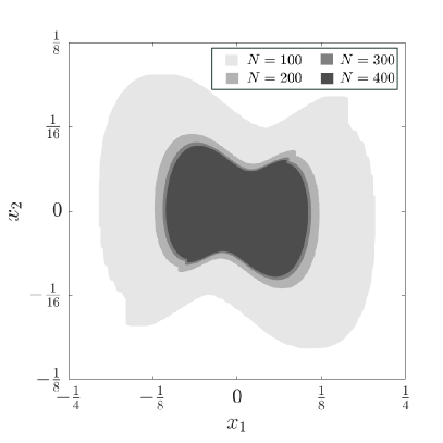
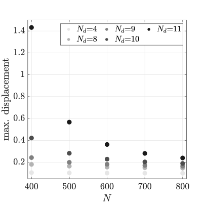
Figure 1: Zonotopic over-approximations computed by the proposed method for the example in Section V, for selected values of the discretization parameters $N$ and $N_{d}$: Reachable tube $\mathcal{R}(\left[t_{0},t_{f}\right])$ for $N_{d}=4$ (left), and maximum bridge displacement, upon all nodal points, obtained from reachable tube $\mathcal{R}(\left[t_{0},t_{f}\right])$, for $N_{d}\in\{4,8,9,10,11\}$ (right).

To close this section, we discuss the complexity of the proposed method. It is easily seen that the memory requirement of algorithm ( ‣ IV-B is determined by the need to store the computed zonotopic over-approximation. The zonotope $\Lambda_{i}^{N}$, $i\in\left[1;N\right]$, obtained in Theorem IV.7, has $2p+1+(2i-1)(q+n)$ generators, and consequently, the over-approximation $\widehat{R}_{N}$ obtained in Corollary IV.8 consists of $N$ zonotopes in $\mathbb{R}^{n}$ with a total of $(q+n)N^{2}+(2p+1)N$ generators. In particular, the memory required by the zonotopic over-approximation, and in turn, the memory required by our method, is of order $O(n^{2}N^{2})$ as one of the variables $n$ or $N$ tends to infinity and the other one is fixed, where we have assumed both $p=O(n)$ and $q=O(n)$. Regarding the run time of algorithm ( ‣ IV-B, we additionally assume $m=O(n)$ and consider only arithmetic operations. Then the computational effort is dominated by the multiplication of an $n\times n$ matrix by an $n\times(p+(i-1)(q+n))$ matrix in step ( ‣ ( ‣ IV-B. Hence, the run time of algorithm ( ‣ IV-B is of order $O(n^{3}N^{2})$ as one of the variables $n$ or $N$ tends to infinity and the other one is fixed.

V Numerical Example

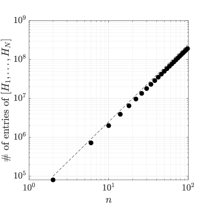
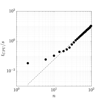
Figure 2: Performance of the proposed method on the example in Section V for the time discretization parameter $N=100$, depending on the dimension $n$ of the state space of the system ( ‣ I: Total number of components of the generators of the computed zonotopic over-approximation (left), and run time (right).

In this section, we demonstrate the performance of the proposed method on a comprehensive numerical example. Specifically, we consider several instances of a reduced order model, obtained by finite difference approximation, of an infinite dimensional pedestrians-footbridge system.

V-A Footbridge Model

Analyzing the dynamic response of footbridges is crucial for their structural integrity and the safety of pedestrians [33, 34]. In this example, we consider a continuum model of a pedestrians-footbridge system. The pedestrians’ stroll on the footbridge generates dynamic load which triggers deformation of the footbridge. The lateral displacement of the footbridge is given by the function $q\colon\mathcal{I}\times\left[0,L\right]\rightarrow\mathbb{R}$, where $L$ denotes the length of the bridge, and $\mathcal{I}=\left[t_{0},t_{f}\right]$ is the compact time interval under consideration. Let $\mathcal{S}=\mathcal{I}\times\left[0,L\right]$. The function $q$ satisfies (see, e.g. [33, eq. 29][34, eqs. 2.91, 2.92][35, eq. 2])

$$mD_{1}^{2}q +EID_{2}^{4}q+cD_{1}q=f_{p}(t,y),\leavevmode\nobreak\ (t,y)\in\mathcal{S},$$ (18a)

$$f_{p}(t,y) =f_{0}\cos(\omega t)q(t,y)+w(t,y),\leavevmode\nobreak\ (t,y)\in\mathcal{S},$$ (18b)

$$\left|w(t,y)\right| \leq\bar{w},(t,y)\in\mathcal{S},$$ (18c)

$$q(t,0) =q(t,L)=D_{2}^{2}q(t,0)=D_{2}^{2}q(t,L)=0,\leavevmode\nobreak\ t\in\mathcal{I},$$ (18d)

$$q(t_{0},y) =D_{1}q(t_{0},y)=0,\leavevmode\nobreak\ y\in\left[0,L\right],$$ (18e)

where $D_{i}^{k}q$ denotes the $k$th order partial derivative of the map $q$ w.r.t. its $i$th argument, $D_{1}\mathrel{:=}D_{1}^{1}$, $m$ denotes the mass per unit length, $EI$ is the bending stiffness, $c$ is a damping coefficient, $f_{p}(t,y)$ is the load per unit length, $f_{0}$ and $\omega$ are model parameters, $w(t,y)$ is a bounded uncertain term, and $\bar{w}\in\mathbb{R}_{+}$ is the bound on the uncertainty.

V-B Reduced Order Model

Now, we deduce a reduced order model from system ( ‣ V-A by means of finite difference. Let $N_{d}$ be a spatial discretization parameter with $N_{d}\geq 4$, and $h_{y}\mathrel{:=}L/N_{d}$, $y_{i}\mathrel{:=}ih_{y}$, $i\in\left[0;N_{d}\right]$. By replacing the $4$th order spatial derivative in ( ‣ ( ‣ V-A with second order centered difference (see, e.g. [36]), and the second order spacial derivatives in ( ‣ ( ‣ V-A with first order forward and backward differences, respectively, and considering the homogeneous boundary and initial conditions in ( ‣ ( ‣ V-A and ( ‣ ( ‣ V-A, we obtain the approximating model $m\ddot{z}+K(t)z+c\dot{z}=v(t),$ where $z(0)=\dot{z}(0)=0$, $v(t)\in\left[-\bar{w},\bar{w}\right]^{N_{d}-3}$, $t\in\left[t_{0},t_{f}\right]$, and $K(\cdot)$ is obtained from the finite difference approximation. By setting $x=(z,\dot{z})$, we arrive at a problem for system ( ‣ I, where

$$A(t) =\left(\begin{array}[]{cc}0&\operatorname{id}\\ -\frac{1}{m}K(t)&-\frac{c}{m}\operatorname{id}\end{array}\right)\text{\ \ and\ \ }B=\left(\begin{array}[]{c}0\\ \operatorname{id}\end{array}\right),$$ (19e)

$$U =\left[-\bar{w}/m,\bar{w}/m\right]^{N_{d}-3},\leavevmode\nobreak\ X_{0}=\{0\}.$$ (19f)

The dimension of the system ( ‣ I is $n=2(N_{d}-3)$. We note that system ( ‣ V-B, for the case $N_{d}=4$, corresponds to a damped and perturbed version of the well-known Mathieu equation which models various physical phenomena and engineering systems; see, e.g. [26]. We also note that the approach followed above to obtain the reduced order linear time-varying (LTV) problem ( ‣ V-B from ( ‣ V-A has been followed in the literature to construct benchmark problems for reachability analysis of linear time-invariant (LTI) systems [37]. In this example, we set $L=10$, $m=2$, $c=f_{0}=EI=\omega=1$, $\bar{w}=0.01$, and $\left[t_{0},t_{f}\right]=\left[0,20\right]$. We aim at over-approximating the reachable tube $\mathcal{R}(\left[t_{0},t_{f}\right])$ of ( ‣ I for several instances of $N_{d}$, using the proposed method. The computed over-approximations will be used to obtain bounds on the bridge displacements and will be analyzed in terms of accuracy and computational costs.

V-C Implementation

To address the problem described above, we employ the zonotopic variant of the proposed method as given in ( ‣ IV-B. Moreover, we take advantage of the smoothness of the matrix-valued function $A(\cdot)$ in ( ‣ ( ‣ V-B and use a second order approximation $\tilde{\phi}$ of the transition matrix as given in Lemma .4. The zonotopic variant is implemented in MATLAB (2019a), and MATLAB is run on an AMD Ryzen 5 2500U/ 2GHz processor. Plots of zonotopes are produced with the help of software CORA [38].

V-D Results

First, we demonstrate the over-approximations obtained by the proposed method. Fig. 1 illustrates several over-approximations of $\mathcal{R}(\left[t_{0},t_{f}\right])$, with $N_{d}=4$. As seen in the mentioned figure, the accuracy of the over-approximations increases as the value of $N$ increases, which matches with the findings of this work. Next, bounds on the displacement of the bridge are obtained based on several over-approximations of $\mathcal{R}(\left[t_{0},t_{f}\right])$ for several instances of $N_{d}$. Fig. 1 also illustrates bounds on bridge displacement obtained for several values of $N_{d}$ and $N$. The quality of the bounds improves as $N$ increases due to the increased accuracy of the computed over-approximations.

Finally, the scalability of the proposed method is illustrated by considering a fixed value of the time discretization parameter $N$ and selected values of the spatial discretization parameter $N_{d}$. Fig. 2 indicates a memory requirement of order $O(n^{2})$, as predicted by the discussion at the end of Section IV, and a run time of order $O(n^{2.4})$ approximately, which is less than the predicted $O(n^{3})$. The difference is due to the fact that MATLAB takes advantage of the sparse structure of the matrix $\widetilde{\Phi}$ in Lemma .4, inherited from the matrix $A$ in ( ‣ ( ‣ V-B.

V-E Comparison: Ellipsoidal Techniques

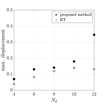
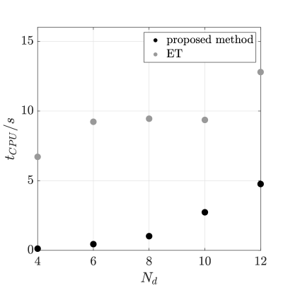
Figure 3: Comparison between the zonotopic variant, with $N=800$, and the ET both applied to the example in Section V for different instances of the discretization parameter $N_{d}$: Estimation of maximum bridge displacement at time $t_{f}$, and run time (right).

In this subsection, we illustrate the performance of the zonotopic variant of the proposed method in comparison with ellipsoidal techniques [5] implemented in the ellipsoidal toolbox (ET) [39].

As we have discussed in the Introduction, ellipsoidal techniques yield reachable tubes only in implicit form, and hence we restrict the scope of the comparison to reachable sets only. Here, we consider different instances of system ( ‣ V-B with $n\in\left[2;18\right]$, or equivalently, $N_{d}\in\left[4;12\right]$. The ellipsoidal set $\tilde{U}\mathrel{:=}(\bar{w}/m)\mathbb{B}_{2}$, where $\mathbb{B}_{2}$ is the $2$-norm closed unit ball in $\mathbb{R}^{N_{d}-3}$, is considered as the input set when applying the ET, as the ET is directly applicable to ellipsoidal initial and input sets only. Since $\tilde{U}\subseteq U$, the ET is given the advantage of using a smaller input set. As the sets $B\tilde{U}$ and $X_{0}$ are degenerate, the ET requires defining a regularization parameter, which we have set to be $10^{-3}$, which introduces full dimensional conservative substitutes. Moreover, we arbitrarily use the direction vector $e_{1}=(1,0,0,\ldots)$ in our computations of ellipsoidal approximations. The zonotopic variant is implemented with $N=800$ and restricted to compute reachable sets only (computations in equations ( ‣ ( ‣ IV-B and ( ‣ ( ‣ IV-B are omitted). Both techniques are set to obtain over-approximations of $\mathcal{R}(t_{f})$ which are subsequently used to estimate the maximum bridge displacement, upon all nodal points, at time $t_{f}$.

Fig. 3 (left) shows that for instances of system ( ‣ V-B, with $N_{d}\in\left[4;12\right]$, the zonotopic variant performs very well in comparison with the ET in terms of estimating maximum bridge displacement despite the inherent disadvantage of using a larger input set and of accounting for approximation errors which are not considered by the ET. As seen from Fig. 3 (left), the effect of these errors is more pronounced for increasing state space dimension, which is due to rapidly growing estimates of matrix norms of the system matrices and their derivatives (growth is of order $O(n^{4})$ as a result of the finite difference approximation of the $4$th order derivative in equation ( ‣ ( ‣ V-A). Fig. 3 (right) illustrates that the zonotopic variant outperforms the ET in terms of computational time for the instances of system ( ‣ V-B, with $N_{d}\in\left[4;12\right]$. We note, however, that the ET computes additionally under-approximations of reachable sets, which might contribute to the relatively higher computational time.

VI Conclusion

We have proposed a method to compute over-approximations of reachable tubes for LTV systems that are additionally represented in a form suitable for formal verification purposes. The method has been inspired by existing techniques for LTI systems, and, when applied to that special case, it is almost equivalent to those in [9, 11], except that it additionally requires to repeatedly compute convex hulls. We have also presented a zonotopic variant of the method and demonstrated its performance on an example, which indicates that the computational effort is comparable to that of existing methods approximating reachable sets rather than tubes. The accuracy of our method could be improved by implementing component-wise estimates as in e.g. [12], in place of matrix and vector norms.

.1 Lemma (Convex Sets).

Let $\Omega,\Gamma\subseteq\mathbb{R}^{n}$ be convex, $\alpha,\beta\in\mathbb{R}$, and $L\in\mathbb{R}^{m\times n}$. Then the following holds.

1. The sets $\alpha\Omega$, $\Omega+\Gamma$ and $L\Omega$ are convex. They are additionally compact if $\Omega$ and $\Gamma$ are so.

2. If $\Omega$ and $\Gamma$ are additionally non-empty, then $\mathop{\rm conv}\nolimits(\Omega\cup\Gamma)=\left\{\lambda x+(1-\lambda)y\,\middle|\,x\in\Omega,y\in\Gamma,\lambda\in\left[0,1\right]\right\}$. ∎

Proof.

For (i), see [40, Sect. 3] and note that images of compact sets under continuous maps are compact. For (ii), see [40, Th. 3.3]. ∎

The Hausdorff distance $d_{H}(\Omega,\Gamma)$ of two non-empty bounded subsets $\Omega,\Gamma\subseteq\mathbb{R}^{n}$ w.r.t. $\|\cdot\|$ is defined by

$$d_{H}(\Omega,\Gamma)=\inf\left\{\varepsilon>0\,\middle|\,\Omega\subseteq\Gamma+\varepsilon\mathbb{B},\Gamma\subseteq\Omega+\varepsilon\mathbb{B}\right\},$$

and is used to measure the extent by which the two sets $\Omega$ and $\Gamma$ differ from each other. This distance satisfies the triangle inequality, it is a metric when restricted to non-empty compact subsets of $\mathbb{R}^{n}$ [41], and it additionally enjoys the properties in the following lemma.

.2 Lemma (Hausdorff Distance).

Let $\Omega,\Omega^{\prime},\Gamma,\Gamma^{\prime}\subseteq\mathbb{R}^{n}$ be non-empty and bounded, and let $A,B\in\mathbb{R}^{m\times n}$ and $\delta,\varepsilon\in\mathbb{R}_{+}$. Then the following holds:

1. $d_{H}(\Omega+\Gamma,\Omega^{\prime}+\Gamma^{\prime})\leq d_{H}(\Omega,\Omega^{\prime})+d_{H}(\Gamma,\Gamma^{\prime})$.

2. $d_{H}(A\Omega,A\Gamma)\leq\|A\|d_{H}(\Omega,\Gamma)$.

3. $d_{H}(A\Omega,B\Omega)\leq\|A-B\|\|\Omega\|$.

4. $\|\Omega\|=d_{H}(\Omega,\{0\})$.

5. If $\Omega$ and $\Gamma$ are additionally closed, then $d_{H}(\Omega,\Gamma)\leq\varepsilon$ iff $\Omega\subseteq\Gamma+\varepsilon\mathbb{B}$ and $\Gamma\subseteq\Omega+\varepsilon\mathbb{B}$.

6. If $d_{H}(\Omega,\Gamma)\leq\varepsilon$, then $d_{H}(\Omega,\Gamma+\delta\mathbb{B})\leq\varepsilon+\delta$.

7. Let $(\Omega_{i})_{i\in I}$ and $(\Gamma_{i})_{i\in I}$ be families of non-empty subsets of $\mathbb{R}^{n}$. Then $d_{H}\left(\cup_{i\in I}\Omega_{i},\cup_{i\in I}\Gamma_{i}\right)\leq\sup_{i\in I}d_{H}(\Omega_{i},\Gamma_{i})$.

Proof.

For (i), (iii) and (v), see [41, Lemma 2.2], [25, Lemma 0.1.2.7], and the discussion in [42, p. 48]. The definition of $d_{H}$ directly implies (ii) and (iv), and (i) and (iv) imply (vi). To prove (vii), we may assume that $\sup_{i\in I}d_{H}(\Omega_{i},\Gamma_{i})<\varepsilon$ for some real $\varepsilon$. Then $d_{H}(\Omega_{i},\Gamma_{i})<\varepsilon$ for every $i\in I$, and in turn $\Omega_{i}\subseteq\varepsilon\mathbb{B}+\Gamma_{i}$. It follows that $\cup_{i\in I}\Omega_{i}\subseteq\varepsilon\mathbb{B}+\cup_{i\in I}\Gamma_{i}$, and similarly with the roles of $\Omega_{i}$ and $\Gamma_{i}$ interchanged. Hence, $d_{H}\left(\cup_{i\in I}\Omega_{i},\cup_{i\in I}\Gamma_{i}\right)\leq\varepsilon$, and since the bound $\varepsilon$ was arbitrary, we are done. ∎

In the following result, given a norm $\|\cdot\|$ on $\mathbb{R}^{n}$, it is assumed that the norm of any matrix $A\in\mathbb{R}^{n\times p}$ is w.r.t. the maximum norm on $\mathbb{R}^{p}$, i.e., $\|A\|=\sup\left\{\|Ax\|\,\middle|\,\|x\|_{\infty}\leq 1\right\}$.

.3 Lemma (Zonotopes).

Let $b,c\in\mathbb{R}^{n}$, $F\in\mathbb{R}^{n\times p}$, $G\in\mathbb{R}^{n\times q}$, and $L\in\mathbb{R}^{m\times n}$, and denote $\Omega={\bar{Z}}(b,F)$, $\Gamma={\bar{Z}}(c,G)$. Then the following holds.

1. $\Omega+\Gamma={\bar{Z}}(b+c,(F,G))$, where $(F,G)\in\mathbb{R}^{n\times(p+q)}$.

2. $L\Gamma={\bar{Z}}(Lc,LG)$.

3. $\|\Gamma\|=\|(c,G)\|$, where $(c,G)\in\mathbb{R}^{n\times(q+1)}$. In particular, $\|\Gamma\|_{\infty}=\max\left\{|c_{i}|+\sum_{j=1}^{q}|G_{i,j}|\,\middle|\,i\in\left[1;n\right]\right\}$.

4. If $p=q$, then $\mathop{\rm conv}\nolimits(\Omega\cup\Gamma)\subseteq{\bar{Z}}\left(\mathop{\rm Enc}\nolimits((b,F),(c,G))\right)$, where the operator $\mathop{\rm Enc}\nolimits$ is defined in ( ‣ IV-B. Moreover, the Hausdorff distance between the two sets does not exceed $\|F-G\|$. In particular, for the Hausdorff distance w.r.t. the maximum norm, the bound equals $\max\left\{\sum_{j=1}^{q}|F_{i,j}-G_{i,j}|\,\middle|\,i\in\left[1;n\right]\right\}$.

Proof.

For (i) and (ii), see [43, Prop. 1.4, 1.5]. To prove (iii), note that $\|{\bar{Z}}(0,(c,G))\|=\|(c,G)\|$ by the very definition ( ‣ IV-B of ${\bar{Z}}$, and that $\Gamma\subseteq{\bar{Z}}(0,(c,G))$. It remains to show that $\|{\bar{Z}}(0,(c,G))\|\leq\|\Gamma\|$. To this end, let $p=\alpha c+y$ for some $\alpha\in\left[-1,1\right]$ and $y\in G\left[-1,1\right]^{q}$. Then $p=\lambda(c+y)+(1-\lambda)(y-c)$ for $\lambda=(1+\alpha)/2\in\left[0,1\right]$, and so $\|p\|\leq\max\{\|c+y\|,\|c-y\|\}$ as $\|\cdot\|$ is convex. It follows that $\|p\|\leq\|\Gamma\|$ since $c+y,c-y\in\Gamma$. The set inclusion claim in (iv) is known [9]; we sketch a proof: Denote $E={\bar{Z}}(\mathop{\rm Enc}\nolimits((b,F),(c,G)))$ and let $x=b+F\lambda$ for some $\lambda\in\left[-1,1\right]^{p}$. Then $x=(b+c)/2+(b-c)/2+(F+G)\lambda/2+(F-G)\lambda/2\in E$. This shows that $\Omega\subseteq E$, and similarly we obtain $\Gamma\subseteq E$. The claim follows as $E$ is convex. To prove the estimate, which improves Girard’s result [9], let $x\in E$. Then $2x=b+c+\alpha(b-c)+(F+G)\mu+(F-G)\nu$ for some $\alpha\in\left[-1,1\right]$ and some $\mu,\nu\in\left[-1,1\right]^{p}$. Define $y=\lambda(c+G\mu)+(1-\lambda)(b+F\mu)$ for $\lambda=(1-\alpha)/2\in\left[0,1\right]$. Then $y\in\mathop{\rm conv}\nolimits(\Omega\cup\Gamma)$ by Lemma .1(ii), and $x-y=(F-G)(\nu-\alpha\mu)/2$. Since $\|\nu-\alpha\mu\|_{\infty}\leq 2$, we arrive at $\|x-y\|\leq\|F-G\|$, which proves the bound. ∎

.4 Lemma (Taylor’s method of order $\mathbf{2}$).

Suppose that hypotheses ($H_{1}$)-($H_{3}$) in Section III hold. Additionally assume that $A$ is of class $C^{2}$ and that $\|\ddot{A}(t)\|\leq M_{\ddot{A}}$ holds for all $t\in\left[t_{0},t_{f}\right]$. Define $\widetilde{\phi}\colon D\to\mathbb{R}^{n\times n}$ by $\widetilde{\phi}(t,s)=\operatorname{id}+(t-s)A(s)+(t-s)^{2}(\dot{A}(s)+A(s)^{2})/2$. Then condition ($H_{4}$) in Section III holds with $\theta$ given by $\theta(h)=(1+3M_{\dot{A}}/M_{A}^{2}+M_{\ddot{A}}/M_{A}^{3})(\exp(hM_{A})-h^{2}M_{A}^{2}/2-hM_{A}-1)$.

Proof.

The map $\theta$ is clearly monotonically increasing, and $\theta(h)=O(h^{3})$ as $h\to 0$, which implies ( ‣ ($H_{4}$). Given $s\in\left[t_{0},t_{f}\right]$, Taylor’s formula for $\phi(\cdot,s)$ about the point $s$ reads $\phi(t,s)=\widetilde{\phi}(t,s)+\frac{1}{2}(t-s)^{3}\int_{0}^{1}(1-z)^{2}D_{1}^{3}\phi(s+z(t-s),s)dz$. Using the identity $D_{1}^{3}\phi(t,s)=(\ddot{A}(t)+2A(t)\dot{A}(t)+\dot{A}(t)A(t)+A(t)^{3})\phi(t,s)$ as well as the estimate ( ‣ II-B we obtain the estimate ( ‣ ($H_{4}$). ∎

References

- [1] G. Basile and G. Marro, Controlled and conditioned invariants in linear system theory. Englewood Cliffs, NJ: Prentice Hall Inc., 1992.
- [2] F. Blanchini and S. Miani, Set-theoretic methods in control, ser. Systems & Control: Foundations & Applications. Boston, MA: Birkhäuser Boston Inc., 2008.
- [3] P. Tabuada, Verification and control of hybrid systems. Springer, 2009.
- [4] M. Althoff, S. Bak, M. Forets, G. Frehse, N. Kochdumper, R. Ray, C. Schilling, and S. Schupp, “ARCH-COMP19 Category Report: Continuous and hybrid systems with linear continuous dynamics,” in Proc. 6th Intl. Worksh. Appl. Verification for Continuous and Hybrid Systems (ARCH), ser. EPiC Series in Computing, G. Frehse and M. Althoff, Eds., vol. 61. EasyChair, 2019, pp. 14–40.
- [5] A. B. Kurzhanski and P. Varaiya, Dynamics and control of trajectory tubes, ser. Systems & Control: Foundations & Applications. Birkhäuser/Springer, 2014, theory and computation.
- [6] G. Reissig, A. Weber, and M. Rungger, “Feedback refinement relations for the synthesis of symbolic controllers,” IEEE Trans. Automat. Control, vol. 62, no. 4, pp. 1781–1796, Apr. 2017. doi:10.1109/TAC.2016.2593947
- [7] M. Althoff, “Reachability analysis of large linear systems with uncertain inputs in the Krylov subspace,” IEEE Trans. Automat. Control, vol. 65, no. 2, pp. 477–492, 2020.
- [8] T. Pecsvaradi and K. S. Narendra, “Reachable sets for linear dynamical systems,” Inform. and Control, vol. 19, pp. 319–344, 1971.
- [9] A. Girard, “Reachability of uncertain linear systems using zonotopes,” in Proc. 8th Intl. Workshop on Hybrid Systems: Computation and Control (HSCC), Zürich, Switzerland, Mar. 9-11, 2005, ser. Lect. Notes Comput. Sci., M. Morari and L. Thiele, Eds., vol. 3414. Springer, 2005, pp. 291–305.
- [10] A. Girard, C. Le Guernic, and O. Maler, “Efficient computation of reachable sets of linear time-invariant systems with inputs,” in Proc. 9th Intl. Workshop on Hybrid Systems: Computation and Control (HSCC), Santa Barbara, CA, U.S.A., Mar. 29-31, 2006, ser. Lect. Notes Comput. Sci., J. Hespanha and A. Tiwari, Eds. Berlin: Springer, 2006, vol. 3927, pp. 257–271.
- [11] C. Le Guernic and A. Girard, “Reachability analysis of linear systems using support functions,” Nonlinear Anal. Hybrid Syst., vol. 4, no. 2, pp. 250–262, 2010.
- [12] G. Frehse, C. Le Guernic, A. Donzé, S. Cotton, R. Ray, O. Lebeltel, R. Ripado, A. Girard, T. Dang, and O. Maler, “SpaceEx: scalable verification of hybrid systems,” in Proc. 23rd Intl. Conf. Computer Aided Verification (CAV), Snowbird, UT, USA, Jul.14-20, 2011, ser. Lect. Notes Comput. Sci., vol. 6806. Springer, Heidelberg, 2011, pp. 379–395.
- [13] M. Althoff and G. Frehse, “Combining zonotopes and support functions for efficient reachability analysis of linear systems,” in Proc. IEEE Conf. Decision and Control (CDC), Las Vegas, U.S.A., 12-14 Dec. 2016, 2016, pp. 7439–7446.
- [14] M. Althoff, B. H. Krogh, and O. Stursberg, “Analyzing reachability of linear dynamic systems with parametric uncertainties,” in Modeling, design, and simulation of systems with uncertainties, ser. Math. Eng. Springer, Heidelberg, 2011, pp. 69–94.
- [15] O. Botchkarev and S. Tripakis, “Verification of hybrid systems with linear differential inclusions using ellipsoidal approximations,” in Proc. 3rd Intl. Workshop on Hybrid Systems: Computation and Control (HSCC), Pittsburgh, U.S.A., Mar. 23-25, 2000, ser. Lect. Notes Comput. Sci., N. A. Lynch and B. H. Krogh, Eds., vol. 1790. Springer, 2000, pp. 73–88.
- [16] M. E. Villanueva, R. Quirynen, M. Diehl, B. Chachuat, and B. Houska, “Robust MPC via min-max differential inequalities,” Automatica J. IFAC, vol. 77, pp. 311–321, 2017.
- [17] M. Serry and G. Reissig, “Hyper-rectangular over-approximations of reachable sets for linear uncertain systems,” in Proc. 57th IEEE Conf. Decision and Control (CDC), Miami, FL, USA, 17-19 Dec. 2018, 2018, pp. 6275–6282. doi:10.1109/CDC.2018.8619276
- [18] K. Shen and J. K. Scott, “Exploiting nonlinear invariants and path constraints to achieve tighter reachable set enclosures using differential inequalities,” Math. Control Signals Systems, vol. 32, no. 1, pp. 101–127, 2020.
- [19] M. Zamani, G. Pola, M. Mazo, Jr., and P. Tabuada, “Symbolic models for nonlinear control systems without stability assumptions,” IEEE Trans. Automat. Control, vol. 57, no. 7, pp. 1804–1809, 2012.
- [20] N. S. Nedialkov, K. R. Jackson, and G. F. Corliss, “Validated solutions of initial value problems for ordinary differential equations,” Appl. Math. Comput., vol. 105, no. 1, pp. 21–68, 1999.
- [21] V. Veliov, “Second-order discrete approximation to linear differential inclusions,” SIAM Journal on Numererical Analysis, vol. 29, no. 2, pp. 439–451, 1992.
- [22] W.-J. Beyn and J. Rieger, “Numerical fixed grid methods for differential inclusions,” Computing, vol. 81, no. 1, pp. 91–106, 2007.
- [23] G. Reissig and M. Rungger, “Symbolic optimal control,” IEEE Trans. Automat. Control, vol. 64, no. 6, pp. 2224–2239, Jun. 2019. doi:10.1109/TAC.2018.2863178
- [24] S. Bak and P. S. Duggirala, “Simulation-equivalent reachability of large linear systems with inputs,” in Computer aided verification. Part I, ser. Lect. Notes Comput. Sci. Springer, 2017, vol. 10426, pp. 401–420.
- [25] R. Baier, “Set-valued integration and the discrete approximation of reachable sets,” doctoral thesis, Univ. Bayreuth, Bayreuth, Germany, 1995, (“Mengenwertige Integration und die diskrete Approximation erreichbarer Mengen”, in German).
- [26] T. I. Fossen and H. Nijmeijer, Eds., Parametric resonance in dynamical systems. Springer, New York, 2012, proc. Workshop held in Longyearbyen, Jun. 22–26, 2011.
- [27] N. G. de Bruijn, Asymptotic methods in analysis, 3rd ed. Dover, 1981, corr. reprint.
- [28] D. L. Lukes, Differential equations, ser. Mathematics in Science and Engineering. London: Academic Press Inc., 1982, vol. 162.
- [29] H. Hermes, “The generalized differential equation ,” Advances in Math., vol. 4, pp. 149–169, 1970.
- [30] F. L. Chernous′ko, State Estimation of Dynamic Systems. CRC Press, 1994.
- [31] P. Deuflhard and F. Bornemann, Scientific computing with ordinary differential equations, ser. Texts in Applied Mathematics. Springer-Verlag, New York, 2002, vol. 42.
- [32] C. Le Guernic, “Reachability analysis of hybrid systems with linear continuous dynamics,” Ph.D. dissertation, Université Grenoble I - Joseph Fourier, 28 Oct. 2009.
- [33] G. Piccardo and F. Tubino, “Parametric resonance of flexible footbridges under crowd-induced lateral excitation,” J. Sound Vibration, vol. 311, no. 1-2, pp. 353–371, 2008.
- [34] F. Gazzola, Mathematical models for suspension bridges. Springer, 2015.
- [35] J. Bodgi, S. Erlicher, and P. Argoul, “Lateral vibration of footbridges under crowd-loading: Continuous crowd modeling approach,” in Key Engineering Materials, vol. 347. Trans Tech Publ, 2007, pp. 685–690.
- [36] B. Fornberg, “Generation of finite difference formulas on arbitrarily spaced grids,” Math. Comp., vol. 51, no. 184, pp. 699–706, 1988.
- [37] H.-D. Tran, L. V. Nguyen, and T. T. Johnson, “Large-scale linear systems from order-reduction,” in Proc. 3rd Intl. Worksh. Appl. Verification for Continuous and Hybrid Systems (ARCH), ser. EPiC Series in Computing, G. Frehse and M. Althoff, Eds., vol. 43. EasyChair, 2017, pp. 60–67.
- [38] M. Althoff, “An introduction to CORA 2015,” in Proc. 1st and 2nd Intl. Worksh. Appl. Verification for Continuous and Hybrid Systems (ARCH), ser. EPiC Series in Computing, G. Frehse and M. Althoff, Eds., vol. 34. EasyChair, 2015, pp. 120–151.
- [39] P. Gagarinov and A. A. Kurzhanskiy, “Ellipsoidal toolbox release 2.0.1,” UC Berkeley, Dept EECS, Tech. Rep., May 2014. http://systemanalysisdpt-cmc-msu.github.io/ellipsoids/
- [40] R. T. Rockafellar, Convex analysis, ser. Princeton Mathematical Series, No. 28. Princeton, N.J., U.S.A.: Princeton University Press, 1970.
- [41] F. S. De Blasi, “On the differentiability of multifunctions,” Pacific J. Math., vol. 66, no. 1, pp. 67–81, 1976.
- [42] R. Schneider, Convex bodies: the Brunn-Minkowski theory, ser. Encyclopedia of Mathematics and its Applications. Cambridge University Press, Cambridge, 1993, vol. 44.
- [43] V. T. H. Le, C. Stoica, T. Alamo, E. F. Camacho, and D. Dumur, Zonotopes. Wiley, 2013.