An application of a pseudo-parabolic modeling to texture image recognition

Abstract

In this work, we present a novel methodology for texture image recognition using a partial differential equation modeling. More specifically, we employ the pseudo-parabolic Buckley-Leverett equation to provide a dynamics to the digital image representation and collect local descriptors from those images evolving in time. For the local descriptors we employ the magnitude and signal binary patterns and a simple histogram of these features was capable of achieving promising results in a classification task. We compare the accuracy over well established benchmark texture databases and the results demonstrate competitiveness, even with the most modern deep learning approaches. The achieved results open space for future investigation on this type of modeling for image analysis, especially when there is no large amount of data for training deep learning models and therefore model-based approaches arise as suitable alternatives.

1 Introduction

Texture images (also known as visual textures) can be informally defined as those images in which the most relevant information is not encapsulated within one or a limited set of well-defined objects, but rather all pixels share the same importance in their description. This type of image has found numerous application in material sciences [18], medicine [10], facial recognition [14], remote sensing [32], cybersecurity [26], and agriculture [23] to name but a few fields with increasing research activity.

While deep learning approaches have achieved remarkable success in problems of object recognition and variations of convolutional neural networks have prevailed in the state-of-the-art for this task, texture recognition on the other hand still remains a challenging problem and the classical paradigm of local image encoders still is competitive with the most modern deep neural networks, presenting some advantages over the last ones, like the fact that they can work well even when there is little data available for training.

In this context, here we present a local texture descriptor based on the action of an operator derived from the Buckley-Leverett partial differential equation (PDE) (see [1, 2] and references cited therein). PDE models have been employed in computer vision at least since the 1980’s, especially in image processing. The scale-space theory developed by Witkin [30] and Koenderink [16] are remarkable examples of such applications. The anisotropic diffusion equation of Perona and Malik [22] also represented great advancement in that research front, as it solved the problem of edge smoothing, common in classical diffusion models. Evolutions of this model were later presented and a survey on this topic was developed in [29].

Despite these applications of PDEs in image processing, substantially less research has been devoted to recognition. As illustrated in [28], pseudo-parabolic PDEs are promising models for this purpose. An important characteristic of these models is that jump discontinuities in the initial condition are replicated in the solution [9]. This is an important feature in recognition as it allows some control over the smoothing effect and would preserve relevant edges, which are known to be very important in image description.

Based on this context, we propose the use of Buckley-Leverett equation as an operator acting as a nonlinear filter over the texture image. That image is used as initial condition for the PDE problem and the solution obtained by a numerical scheme developed in [1] is used to compose the image representation. The solution at each time is encoded by a local descriptor. Extending the idea presented in [28], here we propose two local features: the sign and the magnitude binary patterns [12]. The final texture descriptors are provided by simple concatenation of histograms over each time.

The effectiveness of the proposed descriptors is validated on the classification of well established benchmark texture datasets, more exactly, KTH-TIPS-2b [13] and UIUC [17]. The accuracy is compared with the state-of-the-art in texture recognition, including deep learning solutions, and the results demonstrate the potential of our approach, being competitive with the most advanced solutions recently published on this topic.

2 Partial differential equation and numerical modeling

We consider an advanced simulation approach for the pseudo-parabolic PDE

$$\frac{\partial u}{\partial t}=\nabla\cdot\mathbf{w},\qquad\text{ where }\qquad\mathbf{w}=g(x,y,t)\,\nabla\left(u+\tau\,\frac{\partial u}{\partial t}\right),$$ (1)

and let $\Omega\subset\mathbb{R}^{2}$ denote a rectangular domain and ${\displaystyle u(\,\cdot\,,\,\cdot\,,\,t):\Omega\rightarrow\mathbb{R}}$ be a sequence of images that satisfies the pseudo-parabolic equation (1), in which the original image at $t=0$ corresponds to the initial condition, along with zero flux condition across the domain boundary $\partial\Omega$, $\mathbf{w}\cdot\mathbf{n}=0,\,(x\,,\,y)\in\partial\Omega$. Following [28] (see also [27, 1]), we consider the discretization modeling of the PDE (1) in a uniform partition of $\Omega$ into rectangular subdomains $\Omega_{i,j}$, for $i=1\,,\,\dots\,,\,m$ and $j=1\,,\,\dots\,,\,l$, with dimensions $\Delta x\times\Delta y$. The center of each subdomain $\Omega_{i,j}$ is denoted by $(x_{i}\,,\,y_{j})$. Given a final time of simulation $T$, consider a uniform partition of the interval $[0\,,\,T]$ into $N$ subintervals, where the time step $\Delta t=T/N$ is subject to a stability condition (see [28, 27] for details). We denote the texture configuration frames in the time levels $t_{n}=n\Delta t$, for $n=0\,,\,\dots\,,\,N$. Let $U_{i,j}^{n}$ and $W_{i,j}^{n+1}$ be a finite difference approximations for $u(x_{i}\,,\,y_{j}\,,\,t_{n})$ and $\mathbf{w}$, respectively, and both related to the pseudo-parabolic PDE modeling of (1). Motivated by our promising results in [28], we employ a stable cell-centered finite difference discretization in space after applying the backward Euler method in time to (1), yielding

$$\frac{U_{i,j}^{n+1}-U_{i,j}^{n}}{\Delta t}=\frac{W_{i+\frac{1}{2},j}^{n+1}-W_{i-\frac{1}{2},j}^{n+1}}{\Delta x}+\frac{W_{i,j+\frac{1}{2}}^{n+1}-W_{i,j-\frac{1}{2}}^{n+1}}{\Delta y}.$$ (2)

Depending on the application as well as the calibration data and texture parameters upon model (1), we will have linear or nonlinear diffusion models for image processing (see, e.g., [22, 5, 29]). As a result of this process the discrete problem (2) would be linear-like $\mathbf{A}^{n}\,\mathbf{U}^{n+1}=\mathbf{b}^{n}$ or nonlinear-like $\mathbf{F}(\mathbf{U}^{n+1})=0$ and several interesting methods can be used (see, e.g., [2, 28, 27, 22, 5, 29]). We would like to point out at this moment that our contribution relies on the PDE modeling of (1) as well as on the calibration data and texture parameters associated to the pseudo-parabolic modeling in conjunction with a fine tunning of the local descriptors for texture image recognition for the pertinent application under consideration. In summary, we have a family of parameter choice strategies that combines pseudo-parabolic modeling with texture image recognition.

Here, we consider the diffusive flux as $g(x\,,\ y\,,\,t)\equiv 1$, which results (1) to be a linear pseudo-parabolic model. For a texture image classification based on a pseudo-parabolic diffusion model to be processed, we just consider that each subdomain $\Omega_{i,j}$ corresponds to a pixel with $\Delta x=\Delta y=1$. As we perform an implicit robust discretization in time (backward Euler), we simply choose the time step $\Delta t=\Delta x$ and the damping coefficient $\tau=5$. More details can be found in [28]; see also [27, 1].

Therefore, this description summarizes the basic key ideas of our computational PDE modeling approach for texture image classification based on a pseudo-parabolic diffusion model (1).

3 Proposed methodology

Inspired by ideas presented in [28] and significantly extending comprehension on that study, here we propose the development of a family of images $\{u_{k}\}_{k=1}^{K}$. These images are obtained by introducing the original image $u_{0}$ as initial condition for the 2D pseudo-parabolic numerical scheme presented in Section 2. $u_{k}$ is the numerical solution at each time $t=t_{k}$. Here, $K=50$ showed to be a reasonable balance between computational performance and description quality.

Following that, we collected two types of local binary descriptors [12] from each $u_{k}$. More exactly, we used sign $LBP\_S_{P,R}^{riu2}$ and magnitude $LBP\_M_{P,R}^{riu2}$ descriptors. In short, the local binary sign pattern $LBP\_S_{P,R}^{riu2}$ for each image pixel with gray level $g_{c}$ and whose neighbor pixels at distance $R$ have intensities $g_{p}$ ($p=1,\cdots,P$) is given by

$$LBP\_S_{P,R}^{riu2}=\left\{\begin{array}[]{ll}\sum_{p=0}^{P-1}H(g_{p}-g_{c})2^{p}&\mbox{if }\mathcal{U}(LBP_{P,R})\geq 2\\ P+1&\mbox{otherwise},\end{array}\right.$$ (3)

where $H$ corresponds to the Heaviside step function ($H(x)=1$ if $x\geq 0$ and $H(x)=0$ if $x<0$) and $\mathcal{U}$ is the uniformity function, defined by

$$\mathcal{U}(LBP_{P,R})=|H(g_{P-1}-g_{c})-H(g_{0}-g_{c})|+\sum_{p=1}^{P-1}|H(g_{p}-g_{c})-H(g_{p-1}-g_{c})|.$$ (4)

Similarly, the magnitude local descriptor is defined by

$$LBP\_M_{P,R}^{riu2}=\left\{\begin{array}[]{ll}\sum_{p=0}^{P-1}t(|g_{p}-g_{c}|,C)2^{p}&\mbox{ \, if \, }\mathcal{U}(LBP_{P,R})\geq 2\\ P+1&\mbox{otherwise},\end{array}\right.$$ (5)

where $C$ is the mean value of $|g_{p}-g_{c}|$ over the whole image and $t$ is a threshold function, such that $t(x,c)=1$ if $x\geq c$ and $t(x,c)=0$, otherwise.

Finally, we compute the histogram $\mathrm{h}$ of $LBP\_S_{P,R}^{riu2}(u_{k})$ and $LBP\_M_{P,R}^{riu2}(u_{k})$ for the following pairs of $(P,R)$ values: $\{(1,8),(2,16),(3,24),(4,24)\}$. The proposed descriptors can be summarized by

$$\mathfrak{D}(u_{0})=\bigcup_{\mbox{type}=\{S,M\}}\bigcup_{\begin{subarray}{c}(P,R)=\{(8,1),\\ (16,2),(24,3),\\ (24,4)\}\end{subarray}}\bigcup_{k=0}^{K}\mathrm{h}(LBP\_\mbox{type}_{P,R}^{riu2}(u_{k})).$$ (6)

To reduce the dimensionality of the final descriptors, we also apply Karhunen-Loève transform [21] before their use as input to the classifier algorithm. The diagram depicted in Figure 1 illustrates the main steps involved in the proposed algorithm.

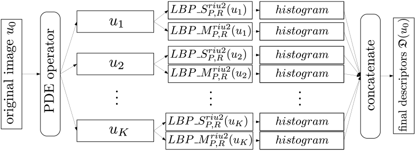
Figure 1: Main steps of the proposed method.

4 Experiments

The performance of the proposed descriptors is assessed on the classification of two well-established benchmark datasets of texture images, namely, KTH-TIPS-2b [13] and UIUC [17].

KTH-TIPS-2b is a challenging database focused on the real material depicted in each image rather than on the texture instance as most classical databases. In this way, images collected under different configurations (illumination, scale and pose) should be part of the same class. The database comprises a total of 4752 color textures with resolution $200\times 200$ (here they are converted to gray scales), equally divided into 11 classes. Each class is further divided into 4 samples (each sample corresponds to a specific configuration). We adopt the most usual (and most challenging) protocol of using one sample for training and the remaining three samples for testing.

UIUC is a gray-scale texture dataset composed by 1000 images with resolution $256\times 256$ evenly divided into 25 classes. The images are photographed under uncontrolled natural conditions and contain variation in illumination, scale, perspective and albedo. For the training/testing split we also follow the most usual protocol, which consists in half of the images (20 per class) randomly selected for training and the remaining half for testing. This procedure is repeated 10 times to allow the computation of an average accuracy.

For the final step of the process, which is the machine learning classifier, we use Linear Discriminant Analysis [11], given its easy interpretation, absence of hyper-parameters to be tuned and known success in this type of application [28].

5 Results and Discussion

Figures 2 and 3 show the average confusion matrices and accuracies (percentage of images correctly classified) for the proposed descriptors in the classification of KTH-TIPS-2b and UIUC, respectively. The average is computed over all training/testing rounds, corresponding, respectively, to 4 rounds in KTH-TIPS-2b and 10 rounds in UIUC. This is an interesting and intuitive graphical representation of the most complicated classes and the most confusable pairs of classes. While in UIUC there is no pair of classes deserving particular attention (the maximum confusion is of one image), KTH-TIPS-2b exhibits a much more challenging scenario. The confusion among classes 3, 5, 8, and 11 is the most critical scenario for the proposed classification framework. It turns out that these classes correspond, respectively, to the materials “corduroy”, “cotton”, “linen”, and “wool”. Despite being different materials, they inevitably share similarities as at the end they are all types of fabrics. Furthermore, looking at the sample from these classes, we can also observe that the attribute “color”, that is not considered here, would be a useful class discriminant in that case. In general, the performance of our proposal in this dataset is quite promising and the confusion matrix and raw accuracy confirm our theoretical expectations.

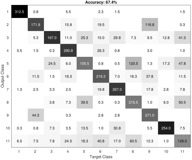
Figure 2: Average confusion matrix and accuracy for KTH-TIPS-2b.

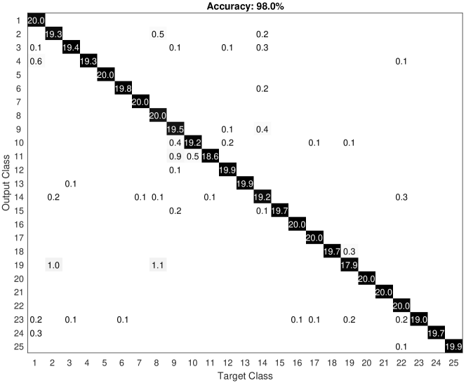
Figure 3: Average confusion matrix and accuracy for UIUC.

Table 1 presents the accuracy compared with other methods in the literature, including several approaches that can be considered as part of the state-of-the-art in texture recognition. First of all, the advantage over the original CLBP, whose part of the descriptors are used here as local encoder, is remarkable, being more than 10% in KTH-TIPS-2b. Other advanced encoders based on SIFT are also outperformed in both datasets (by a large margin in the most challenging textures of KTH-TIPS-2b). SIFT descriptors are complex object descriptors and were considered the state-of-the-art in image recognition for several years. Compared with the most recent CNN-based approaches presented in [8], the results are also competitive. In UIUC, the proposed approach outperforms CNN methods like DeCAF and FC-CNN VGGM. These correspond to complex architectures with a high number of layers and large requirements of computational resources and whose results are pretty hard to be interpreted.

Table 1: Accuracy of the proposed descriptors compared with other texture descriptors in the literature. A superscript ¹ in KTHTIPS-2b means training on three samples and testing on the remainder (no published results for the setup used here).

KTH-TIPS-2b	UIUC
Method Acc. (%) VZ-MR8 [24] 46.3 LBP [20] 50.5 VZ-Joint [25] 53.3 BSIF [15] 54.3 LBP-FH [3] 54.6 CLBP [12] 57.3 SIFT+LLC [8] 57.6 ELBP [19] 58.1 SIFT + KCB [7] 58.3 SIFT + BoVW [7] 58.4 LBPriu2/VAR [20] 58.5 PCANet (NNC) [6] 59.4 RandNet (NNC) [6] 60.7 SIFT + VLAD [7] 63.1 ScatNet (NNC) [4] 63.7 FV-CNN AlexNet [8] 69.7 Proposed 67.4	Method Acc. (%) RandNet (NNC) [6] 56.6 PCANet (NNC) [6] 57.7 BSIF [15] 73.4 VZ-Joint [25] 78.4 LBPriu2/VAR [20] 84.4 LBP [20] 88.4 ScatNet (NNC) [4] 88.6 MRS4 [25] 90.3 SIFT + KCB [7] 91.4 MFS [31] 92.7 VZ-MR8 [24] 92.8 DeCAF [7] 94.2 FC-CNN VGGM [8] 94.5 CLBP [12] 95.7 SIFT+BoVW [7] 96.1 SIFT+LLC [8] 96.3 Proposed 98.0

Generally speaking, the proposed method provided results in texture classification that confirm its potential as a texture image model. Indeed that was theoretically expected from its ability of smoothing spurious noise at the same time that preserves relevant discontinuities on the original image. The combination with a powerful yet simple local encoder like CLBP yielded interesting and promising performance neither requiring large amount of data for training nor advanced computational resources. In general, such great performance combined with the straightforwardness of the model, that allows some interpretation of the texture representation based on local homo/heterogeneous patterns, make the proposed descriptors a candidate for practical applications in texture analysis, especially when we have small to medium datasets and excessively complicated algorithms should be avoided.

6 Conclusions

In this study, we investigated the performance of a nonlinear PDE model (pseudo-parabolic) as an operator for the description of texture images. The operator was applied for a number of iterations (time evolution) and a local encoder was collected from each transformed image. The use of a basic histogram to pooling the local encoders was sufficient to provide competitive results.

The proposed descriptors were evaluated over a practical task of texture classification on benchmark datasets and the accuracy was compared with other approaches from the state-of-the-art. Our method outperformed several other local descriptors that follow similar paradigm and even some learning-based algorithms employing complex versions of convolutional neural networks.

The obtained results confirmed our expectations of a robust texture descriptor, explained by its ability of nonlinearly smoothing out spurious noise and unnecessary details, but preserving relevant information, especially those conveyed by sharp discontinuities. In general, the results and the confirmation of the theoretical formulation suggest the suitability of applying such model in practice, in tasks of texture recognition that require simple models, easy to be interpreted and that do not require much data for training. This is a common situation in areas like medicine and several others.

References

- [1] Abreu, E., Vieira, J.: Computing numerical solutions of the pseudo-parabolic buckley–leverett equation with dynamic capillary pressure. Math. Comput. Simul. 137, 29–48 (2017)
- [2] Abreu, E., Ferraz, P., Vieira, J.: Numerical resolution of a pseudo-parabolic buckley-leverett model with gravity and dynamic capillary pressure in heterogeneous porous media. Journal of Computational Physics 411, 109395 (2020). https://doi.org/https://doi.org/10.1016/j.jcp.2020.109395, http://www.sciencedirect.com/science/article/pii/S0021999120301698
- [3] Ahonen, T., Matas, J., He, C., Pietikäinen, M.: Rotation invariant image description with local binary pattern histogram fourier features. In: Salberg, A.B., Hardeberg, J.Y., Jenssen, R. (eds.) Image Analysis. pp. 61–70. Springer Berlin Heidelberg, Berlin, Heidelberg (2009)
- [4] Bruna, J., Mallat, S.: Invariant scattering convolution networks. IEEE Transactions on Pattern Analysis and Machine Intelligence 35(8), 1872–1886 (2013)
- [5] Catté, F., Lions, P.L., Morel, J.M., Coll, T.: Image selective smoothing and edge detection by nonlinear diffusion. SIAM Journal on Numerical Analysis 29(1), 182–193 (1992)
- [6] Chan, T., Jia, K., Gao, S., Lu, J., Zeng, Z., Ma, Y.: Pcanet: A simple deep learning baseline for image classification? IEEE Transactions on Image Processing 24(12), 5017–5032 (2015)
- [7] Cimpoi, M., Maji, S., Kokkinos, I., Mohamed, S., Vedaldi, A.: Describing textures in the wild. In: Proceedings of the 2014 IEEE Conference on Computer Vision and Pattern Recognition. pp. 3606–3613. CVPR ’14, IEEE Computer Society, Washington, DC, USA (2014)
- [8] Cimpoi, M., Maji, S., Kokkinos, I., Vedaldi, A.: Deep filter banks for texture recognition, description, and segmentation. International Journal of Computer Vision 118(1), 65–94 (2016)
- [9] Cuesta, C., Pop, I.: Numerical schemes for a pseudo-parabolic burgers equation: discontinuous data and long-time behaviour. J. Comput. Appl. Math. 224, 269–283 (2009)
- [10] Dhivyaa, C.R., Sangeetha, K., Balamurugan, M., Amaran, S., Vetriselvi, T., Johnpaul, P.: Skin lesion classification using decision trees and random forest algorithms. Journal of Ambient Intelligence and Humanized Computing (2020)
- [11] Fisher, R.A.: The use of multiple measurements in taxonomic problems. Annals of Eugenics 7(2), 179–188 (1936)
- [12] Guo, Z., Zhang, L., Zhang, D.: A completed modeling of local binary pattern operator for texture classification. Trans. Img. Proc. 19(6), 1657–1663 (2010)
- [13] Hayman, E., Caputo, B., Fritz, M., Eklundh, J.O.: On the significance of real-world conditions for material classification. In: Pajdla, T., Matas, J. (eds.) Computer Vision - ECCV 2004. pp. 253–266. Springer Berlin Heidelberg, Berlin, Heidelberg (2004)
- [14] Jain, D.K., Zhang, Z., Huang, K.: Multi angle optimal pattern-based deep learning for automatic facial expression recognition. Pattern Recognition Letters 139, 157–165 (2020)
- [15] Kannala, J., Rahtu, E.: Bsif: Binarized statistical image features. In: ICPR. pp. 1363–1366. IEEE Computer Society (2012)
- [16] Koenderink, J.J.: The structure of images. Biological Cybernetics 50(5), 363–370 (1984)
- [17] Lazebnik, S., Schmid, C., Ponce, J.: A sparse texture representation using local affine regions. IEEE Transactions on Pattern Analysis and Machine Intelligence 27(8), 1265–1278 (2005)
- [18] Lin, J., Pappas, T.N.: Structural texture similarity for material recognition. In: 2019 IEEE International Conference on Image Processing (ICIP). pp. 4424–4428. IEEE International Conference on Image Processing ICIP, Inst Elect & Elect Engineers; Inst Elect & Elect Engineers Signal Proc Soc (2019), 26th IEEE International Conference on Image Processing (ICIP), Taipei, TAIWAN, SEP 22-25, 2019
- [19] Liu, L., Zhao, L., Long, Y., Kuang, G., Fieguth, P.: Extended local binary patterns for texture classification. Image Vision Comput. 30(2), 86–99 (2012)
- [20] Ojala, T., Pietikäinen, M., Mäenpää, T.: Multiresolution gray-scale and rotation invariant texture classification with local binary patterns. IEEE Transactions on Pattern Analysis and Machine Intelligence 24(7), 971–987 (2002)
- [21] Pearson, F.K.: Liii. on lines and planes of closest fit to systems of points in space. The London, Edinburgh, and Dublin Philosophical Magazine and Journal of Science 2(11), 559–572 (1901)
- [22] Perona, P., Malik, J.: Scale-space and edge detection using anisotropic diffusion. IEEE Trans. Pattern Anal. Mach. Intell. 12(7), 629–639 (1990)
- [23] Robert Singh, K., Chaudhury, S.: Comparative analysis of texture feature extraction techniques for rice grain classification. IET Image Processing 14(11), 2532–2540 (2020)
- [24] Varma, M., Zisserman, A.: A statistical approach to texture classification from single images. International Journal of Computer Vision 62(1), 61–81 (2005)
- [25] Varma, M., Zisserman, A.: A statistical approach to material classification using image patch exemplars. IEEE Transactions on Pattern Analysis and Machine Intelligence 31(11), 2032–2047 (2009)
- [26] Verma, V., Muttoo, S.K., Singh, V.B.: Multiclass malware classification via first- and second-order texture statistics. Computers & Security 97 (2020)
- [27] Vieira, J., Abreu, E.: Numerical modeling of the two-phase flow in porous media with dynamic capillary pressure. Ph.D. thesis, University of Campinas, Campinas, SP, Brazil (7 2018)
- [28] Vieira, J., Abreu, E., Florindo, J.B.: Texture image classification based on a pseudo-parabolic diffusion model (2020), Available at https://arxiv.org/abs/2011.07173
- [29] Weickert, J.: A review of nonlinear diffusion filtering. In: Proceedings of the First International Conference on Scale-Space Theory in Computer Vision. pp. 3–28. SCALE-SPACE ’97, Springer-Verlag, Berlin, Heidelberg (1997)
- [30] Witkin, A.P.: Scale-space filtering. In: Proceedings of the Eighth International Joint Conference on Artificial Intelligence - Volume 2. pp. 1019–1022. IJCAI’83, Morgan Kaufmann Publishers Inc., San Francisco, CA, USA (1983)
- [31] Xu, Y., Ji, H., Fermüller, C.: Viewpoint invariant texture description using fractal analysis. International Journal of Computer Vision 83(1), 85–100 (2009)
- [32] Zhao, G., Wang, X., Cheng, Y.: Hyperspectral image classification based on local binary pattern and broad learning system. International Journal of Remote Sensing 41(24), 9393–9417 (2020)