A Compositional Atlas of Tractable Circuit Operations:
From Simple Transformations to Complex Information-Theoretic Queries

Abstract

Circuit representations are becoming the lingua franca to express and reason about tractable generative and discriminative models. In this paper, we show how complex inference scenarios for these models that commonly arise in machine learning—from computing the expectations of decision tree ensembles to information-theoretic divergences of deep mixture models—can be represented in terms of tractable modular operations over circuits. Specifically, we characterize the tractability of a vocabulary of simple transformations—sums, products, quotients, powers, logarithms, and exponentials—in terms of sufficient structural constraints of the circuits they operate on, and present novel hardness results for the cases in which these properties are not satisfied. Building on these operations, we derive a unified framework for reasoning about tractable models that generalizes several results in the literature and opens up novel tractable inference scenarios.

1 Introduction

Many core computational tasks in machine learning (ML) and AI involve solving complex integrals, such as expectations, that often turn out to be intractable. A fundamental question then arises: under which conditions do these quantities admit tractable computation? That is, when can we compute them efficiently without resorting to approximations or heuristics? Consider for instance the Kullback-Leibler divergence (KLD) between two distributions $p$ and $q$: $\mathbb{D}_{\mathsf{KL}}({p}\parallel{q})=\int{p}(\boldsymbol{x})\log({p}(\boldsymbol{x})/{q}(\boldsymbol{x}))d\mathbf{X}$. Characterizing its tractability can have important applications in learning, approximate inference (Shih & Ermon, 2020), and model compression (Liang & Van den Broeck, 2017).

This “quest” for tracing the tractability of certain quantities of interest—henceforth called queries—has been carried out several times, often independently, for different model classes in ML and AI, and crucially for each query in isolation. Here, we take a different path and introduce a general framework under which the tractability of many complex queries can be traced in a unified manner.

To do so, we focus on circuit representations (Choi et al., 2020) that guarantee exact computation of integrals of interest if the circuit satisfies specific structural properties. They subsume many generative models—probabilistic circuits such as Chow-Liu trees (Chow & Liu, 1968), hidden Markov models (HMMs) (Rabiner & Juang, 1986), sum-product networks (SPNs) (Poon & Domingos, 2011), and other deep mixture models—as well as discriminative ones—including decision trees (Khosravi et al., 2020; Correia et al., 2020) and deep regressors (Khosravi et al., 2019a)—thus enabling a unified treatment of many inference scenarios.

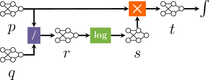
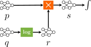
Figure 1: Computational pipelines of the KLD (left) and cross entropy (right) over two distributions $p$ and $q$ encoded as circuits, where the intermediate computations ($r$, $s$ and $t$) are represented as circuits as well.

We represent complex queries as computational pipelines whose intermediate operations transform and combine the input circuits into other circuits. This representation enables us to analyze tractability by “propagating” the sufficient conditions through all intermediate steps. For instance, consider the pipeline for computing the KLD of ${p}$ and ${q}$, two distributions represented by circuits, as shown in Fig. 1. By tracing the tractability conditions of the quotient, logarithm, and product over circuits such that the output circuit (i.e., $t$) admits tractable integration, we can derive a set of minimal sufficient conditions for the input circuits. That is, we can identify a general class of models that supports tractable computation of the KLD.

By re-using the tractability conditions of these simple operations and their algorithms as sub-routines across queries, we are able to compositionally answer many other complex queries. For instance, we can reuse the logarithm and product operations in the KLD pipeline to reason about the tractability of cross entropy (Fig. 1). These sub-routines can be easily implemented in circuit libraries such as Juice (Dang et al., 2021) or SPFlow (Molina et al., 2019).

We make the following contributions. (1) We provide a grammar of simple circuit transformations—products, quotients, powers, logarithms, and exponentials—and introduce sufficient conditions for their tractability while proving their hardness otherwise (Tab. 1); (2) Using this grammar, we unify inference algorithms proposed in the literature for specific representations and extend their scope towards larger model classes; (3) We provide novel tractability and hardness results of complex information-theoretic queries including several widely used entropies and divergences (Tab. 2).

2 Circuit Representations

Circuits represent functions as parameterized computational graphs. By imposing certain structural constraints on these graphs, or verifying their presence, we can guarantee the tractability of certain operations over the encoded functions. As such, circuits provide a language for building and reasoning about tractable representations. We proceed by introducing the basic rules of this language.

We denote random variables by uppercase letters ($X$) and their values/assignments by lowercase ones ($x$). Sets of variables and their assignments are denoted by bold uppercase ($\mathbf{X}$) and bold lowercase ($\boldsymbol{x}$) letters, respectively.

Definition 2.1 (Circuit).

A circuit ${p}$ over variables $\mathbf{X}$ is a parameterized computational graph encoding a function ${p}(\mathbf{X})$ and comprising three kinds of computational units: input, product, and sum. Each inner unit $n$ (i.e., product or sum unit) receives inputs from some other units, denoted $\mathsf{in}(n)$. Each unit $n$ encodes a function ${p}_{n}$ as follows:

$${{p}}_{n}(\mathbf{X})=\begin{cases}l_{n}({\phi(n)})&\text{if $n$ is an input unit}\\ \prod_{c\in\mathsf{in}(n)}{p}_{c}(\mathbf{X})&\text{if $n$ is a product unit}\\ \sum_{c\in\mathsf{in}(n)}\theta_{c}{p}_{c}(\mathbf{X})&\text{if $n$ is a sum unit}\end{cases}$$

where $\theta_{c}\in\mathbb{R}$ are the sum parameters, and input units encode parameterized functions $l_{n}$ over variables $\phi(n)\subseteq\mathbf{X}$, also called their scope. The scope of an inner unit is the union of the scopes of its inputs: $\phi(n)=\bigcup_{c\in\mathsf{in}(n)}\phi(c)$. The output unit of the circuit is the last unit (i.e., with out-degree 0) in the graph, encoding $p(\mathbf{X})$. The support of ${p}$ is the set of all complete states for $\mathbf{X}$ for which the output of ${p}$ is non-zero: $\mathsf{supp}({p})=\{\boldsymbol{x}\in\mathsf{val}(\mathbf{X})\,|\,{p}(\boldsymbol{x})\neq 0\}$.

Circuits can be understood as compact representations of polynomials with possibly an exponential number of terms, whose indeterminates are the functions encoded by the input units. These functions are assumed to be simple enough to allow tractable computations of the operations discussed in this paper. Fig. 2 shows some examples of circuits.

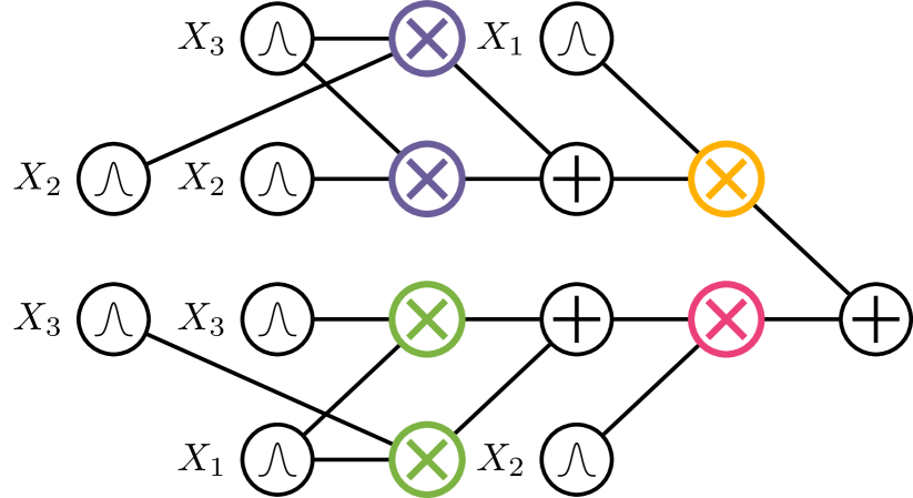
(a) Decomposable

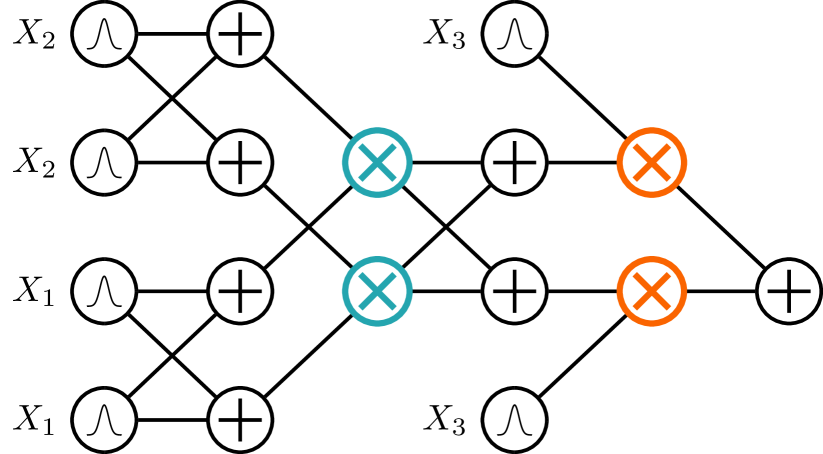
(b) Structured-decomposable

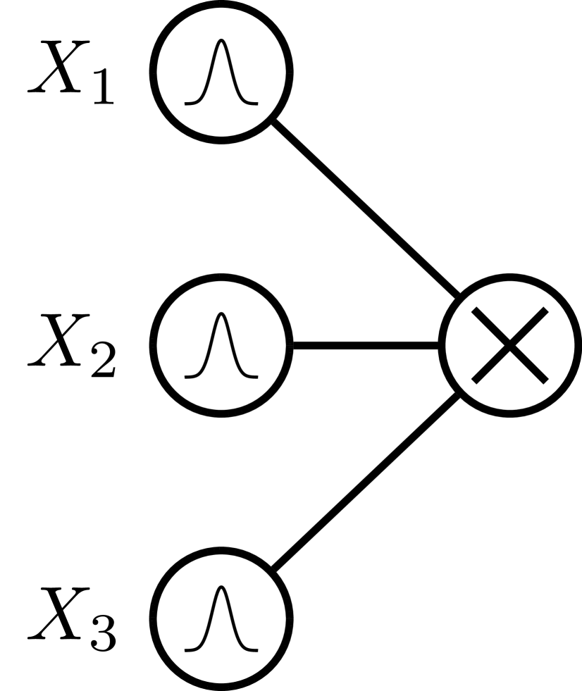
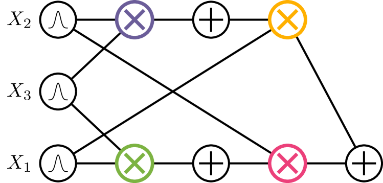
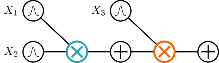
(c) Omni-compatible circuits for $p(\mathbf{X})=p(X_{1})p(X_{2})p(X_{3})$

Figure 2: Examples of circuit representations with different structural properties. The feedforward order is from left to right; input units are labeled by their scope; and sum parameters are omitted for visual clarity. Product units of the rearranged omni-compatible factorization (bottom) are color-coded with those of matching scope in the top circuits.

A probabilistic circuit (PC) (Choi et al., 2020) represents a (possibly unnormalized) probability distribution by encoding its probability mass, density, or a combination thereof.

Definition 2.2 (Probabilistic circuit).

A PC over variables $\mathbf{X}$ is a circuit encoding a function ${p}$ that is non-negative for all values of $\mathbf{X}$; i.e., $\forall\boldsymbol{x}\in\mathsf{val}(\mathbf{X}):p(\boldsymbol{x})\geq 0$.

From here on, we will assume a PC to have positive sum parameters and input units that model valid (unnormalized) distributions, which is a sufficient condition to satisfy the above definition. Moreover, w.l.o.g. we will assume that each layer of a circuit alternates between sum and product units and that every product unit $n$ receives only two inputs, i.e., ${p}_{n}(\mathbf{X})={p}_{c_{1}}(\mathbf{X}){p}_{c_{2}}(\mathbf{X})$. These conditions can easily be enforced on any circuit in exchange for a polynomial increase in its size (Vergari et al., 2015; Peharz et al., 2020).

Computing (functions of) ${p}(\mathbf{X})$, or in other words performing inference, can be done by evaluating its computational graph. Hence, the computational cost of inference on a circuit is a function of its size, defined as the number of edges and denoted as $|{p}|$. For instance, querying the value of ${p}$ for a complete assignment $\boldsymbol{x}$ equals its feedforward evaluation—inputs before outputs—and therefore is linear in $|{p}|$. Other common inference scenarios such as function integration—which translate to marginal inference in the context of probability distributions—can be tackled in linear time with circuits that exhibit certain structural properties, as discussed next.

2.1 Structural Properties of Circuits

Structural constraints on the computational graph of a circuit w.r.t. its scope or support can provide sufficient and/or necessary conditions for certain queries to be computed exactly in polytime. Therefore, one can characterize inference scenarios, also known as classes of queries, in terms of the structural properties realizing these constraints. Moreover, these constraints help understand how circuits generalize several classical tractable model classes, such as mixture models, bounded-treewidth probabilistic graphical models (PGMs), decision trees, and compact logical function representations. It follows that all our results in the following sections automatically translate to these model classes. We now define the structural properties that this work will focus on, referring to Choi et al. (2020) for more details.

Definition 2.3 (Smoothness).

A circuit is smooth if for every sum unit $n$, its inputs depend on the same variables: $\forall\,c_{1},c_{2}\in\mathsf{in}(n),\phi(c_{1})=\phi(c_{2})$.

Smooth PCs generalize homogeneous and shallow mixture models (McLachlan et al., 2019) to deep and hierarchical models. For instance, a Gaussian mixture model (GMM) can be represented as a smooth PC with a single sum unit over as many input units as mixture components, each encoding a (multivariate) Gaussian density.

Definition 2.4 (Decomposability).

A circuit is decomposable if the inputs of every product unit $n$ depend on disjoint sets of variables: $\mathsf{in}(n)=\{c_{1},c_{2}\},\phi(c_{1})\cap\phi(c_{2})=\emptyset$.

Decomposable product units encode local factorizations. That is, a decomposable product unit $n$ over variables $\mathbf{X}$ encodes ${p}_{n}(\mathbf{X})={p}_{1}(\mathbf{X}_{1})\cdot{p}_{2}(\mathbf{X}_{2})$ where $\mathbf{X}_{1}$ and $\mathbf{X}_{2}$ form a partition of $\mathbf{X}$. Taken together, decomposability and smoothness are a sufficient and necessary condition for performing tractable integration over arbitrary sets of variables in a single feedforward pass, as they enable larger integrals to be efficiently decomposed into smaller ones (Choi et al., 2020).

Proposition 2.1 (Tractable integration).

Let ${p}$ be a smooth and decomposable circuit over $\mathbf{X}$ with input functions that can be tractably integrated. Then the integral $\int_{\boldsymbol{z}\in\mathsf{val}(\mathbf{Z})}p(\boldsymbol{y},\boldsymbol{z})d\mathbf{Z}$ can be computed exactly in $\Theta(\left\lvert{p}\right\rvert)$ time for any $\mathbf{Y}\subseteq\mathbf{X},\boldsymbol{y}\in\mathsf{val}(\mathbf{Y}),\mathbf{Z}\!=\!\mathbf{X}\setminus\mathbf{Y}$.

Many complex queries involve integration as the last step. It is therefore convenient that any intermediate operations preserve at least decomposability; smoothness is less of an issue, as it can be enforced in polytime (Shih et al., 2019). Smooth and decomposable PCs with millions of parameters can be efficiently learned from data (Peharz et al., 2020).

A key additional constraint over scope decompositions is compatibility. Intuitively, two decomposable circuits are compatible if they can be rearranged in polynomial time such that their respective product units, once matched by scope, decompose in the same way. We formalize this with the following inductive definition.

Definition 2.5 (Compatibility).

Two circuits ${p}$ and ${q}$ over variables $\mathbf{X}$ are compatible if (1) they are smooth and decomposable and (2) any pair of product units $n\!\in\!{p}$ and $m\!\in\!{q}$ with the same scope can be rearranged into binary products that are mutually compatible and decompose in the same way: $({\phi}(n)\!=\!{\phi}(m))\!\implies\!({\phi}(n_{i})\!=\!{\phi}(m_{i}),\text{ $n_{i}$ and $m_{i}$ are compatible})$ for some rearrangement of the inputs of $n$ (resp. $m$) into $n_{1},n_{2}$ (resp. $m_{1},m_{2}$).

Definition 2.6 (Structured-decomposability).

A circuit is structured-decomposable if it is compatible with itself.

Not all decomposable circuits are structured-decomposable (see Figs. 2(a) and 2(b)), but some can be rearranged to be compatible with any decomposable circuit (see Fig. 2(c)).

Definition 2.7 (Omni-compatibility).

A decomposable circuit ${p}$ over $\mathbf{X}$ is omni-compatible if it is compatible with any smooth and decomposable circuit over $\mathbf{X}$.

For example, in Fig. 2(c), the fully factorized product unit $p(\mathbf{X})=p_{1}(X_{1})p_{2}(X_{2})p_{3}(X_{3})$ can be rearranged into $p_{1}(X_{1})(p_{2}(X_{2})p_{3}(X_{3}))$ and $p_{2}(X_{2})(p_{1}(X_{1})p_{3}(X_{3}))$ to match the yellow and pink products in Fig. 2(a). We can easily see that omni-compatible circuits must assume the form of mixtures of fully-factorized models; i.e., $\sum_{i}\theta_{i}\prod_{j}{p}_{i,j}(X_{j})$. For example, an additive ensemble of decision trees over variables $\mathbf{X}$ can be represented as an omni-compatible circuit (cf. Ex. D.1). Also note that if a circuit is compatible with a non-omni-compatible circuit, then it must be structured-decomposable.

Definition 2.8 (Determinism).

A circuit is deterministic if the inputs $\mathsf{in}(n)$ of every sum unit $n$ have disjoint supports: $\forall\,c_{1},c_{2}\in\mathsf{in}(n),c_{1}\neq c_{2}\implies\mathsf{supp}(c_{1})\cap\mathsf{supp}(c_{2})=\emptyset$.

Analogously to decomposability, determinism induces a recursive partitioning over the support of a circuit. For a deterministic sum unit $n$, the partitioning of its support can be made explicit by introducing an indicator function per each of its inputs, i.e., $\sum_{c\in\mathsf{in}(n)}\theta_{c}{p}_{c}(\boldsymbol{x})=\sum_{c\in\mathsf{in}(n)}\theta_{c}{p}_{c}(\boldsymbol{x})\llbracket{\boldsymbol{x}\in\mathsf{supp}({p}_{c})}\rrbracket$.

Determinism allows for tractable maximization of a circuit (Choi et al., 2020). While we are not investigating maximization in this work, determinism will still play a crucial role in the next sections. Moreover, bounded-treewidth PGMs, such as Chow-Liu trees (Chow & Liu, 1968) and thin junction trees (Bach & Jordan, 2001), can be represented as a smooth, deterministic, and decomposable PC via compilation (Darwiche, 2009; Dang et al., 2020). Probabilistic sentential decision diagrams (PSDDs) (Kisa et al., 2014) are deterministic and structured-decomposable PCs that can be efficiently learned from data (Dang et al., 2020).

Table 1: Tractability and hardness of simple circuit operations. Tractable conditions on inputs translate to conditions on outputs. E.g., consider the quotient of two circuits $p$ and $q$: if they are compatible (Cmp) and $q$ is deterministic (Det), then the output is decomposable (Dec), and deterministic if $p$ is also (+) deterministic and structured-decomposable (SD) if both $p$ and $q$ are. Hardness is for representing the result as a smooth (Sm) and decomposable circuit without some input condition.

Operation		Tractability				Hardness
		Input conditions	Output conditions	Time Complexity
Sum	$\theta_{1}{p}+\theta_{2}{q}$	(+Cmp)	(+SD)	$\mathcal{O}(|{p}|\!+\!|{q}|)$		NP-hard for Det out	(Shen et al., 2016)
Product	${p}\cdot{q}$	Cmp (+Det, +SD)	Dec (+Det, +SD)	$\mathcal{O}(|{p}||{q}|)$	(Thm. B.2)	#P-hard w/o Cmp	(Thm. B.1)
Power	${p}^{n},n\in\mathbb{N}$	SD (+Det)	SD (+Det)	$\mathcal{O}(|{p}|^{n})$	(Thm. B.7)	#P-hard w/o SD	(Thm. B.4 and B.5)
	${p}^{\alpha},\alpha\in\mathbb{R}$	Sm, Dec, Det (+SD)	Sm, Dec, Det (+SD)	$\mathcal{O}(|{p}|)$	(Thm. B.6)	#P-hard w/o Det	(Thm. B.3)
Quotient	${p}/{q}$	Cmp; ${q}$ Det (+$p$ Det,+SD)	Dec (+Det,+SD)	$\mathcal{O}(|{p}||{q}|)$	(Thm. B.9)	#P-hard w/o Det	(Thm. B.8)
Log	$\log({p})$	Sm, Dec, Det	Sm, Dec	$\mathcal{O}(|{p}|)$	(Thm. B.11)	#P-hard w/o Det	(Thm. B.10)
Exp	$\exp(p)$	linear	SD	$\mathcal{O}(\left\lvert{p}\right\rvert)$	(Prop. B.2)	#P-hard	(Thm. B.12)

3 From Simple Circuit Transformations…

This section aims to build and analyze an atlas of simple operations over circuits which can then be composed into more complex operations and queries. Specifically, for each of these operations we are interested in characterizing (1) its tractability in terms of the structural properties of its input circuits, and (2) its closure w.r.t. these properties, i.e. whether they are preserved in the output circuit, while (3) tracing the hardness of representing the output as a decomposable circuit when some property is unmet. Given limited space, we summarize all our main results in Tab. 1 and prove the corresponding statements in the Appendix.

Theorem 3.1.

The tractability and hardness results for simple circuit operations in Tab. 1 hold.

3.1 Sum of Circuits

The simplest operations we can consider are sums and products: a natural choice given that our circuits comprise sum and product units. The operation of summing two circuits ${p}(\mathbf{Z})$ and ${q}(\mathbf{Y})$ is defined as $s(\mathbf{X})=\theta_{1}\cdot{p}(\mathbf{Z})+\theta_{2}\cdot{q}(\mathbf{Y})$ for $\mathbf{X}=\mathbf{Z}\cup\mathbf{Y}$ and two real parameters $\theta_{1},\theta_{2}\in\mathbb{R}$. This operation, which is at the core of additive ensembles of tractable representations, can be realized by introducing a single sum unit that takes as input ${p}$ and ${q}$. Summation applies to any input circuits, regardless of structural assumptions, and it preserves several properties. In particular, if ${p}$ and ${q}$ are decomposable then $s$ is also decomposable; moreover, if they are compatible then $s$ is structured-decomposable as well as compatible with ${p}$ and ${q}$. However, representing a sum as a deterministic circuit is known to be NP-hard (Shen et al., 2016), even for compatible and deterministic inputs.

3.2 Product of Circuits

Multiplication is at the core of many of the compositional queries in Sec. 4. The product of two circuits ${p}(\mathbf{Z})$ and ${q}(\mathbf{Y})$ can be expressed as ${m}(\mathbf{X})={p}(\mathbf{Z})\cdot{q}(\mathbf{Y})$ for variables $\mathbf{X}=\mathbf{Z}\cup\mathbf{Y}$. If $\mathbf{Z}$ and $\mathbf{Y}$ are disjoint, the product $m$ is already decomposable. Shen et al. (2016) proved that representing the product of two decomposable circuits as a decomposable circuit is NP-hard, even if they are deterministic. We prove in Thm. B.1 that it is #P-hard even for structured-decomposable and deterministic circuits.

Recently, Shen et al. (2016) introduced an efficient algorithm for the product of two compatible, deterministic PCs (namely PSDDs). We prove that compatibility alone is sufficient for tractable product computation of any two circuits (Thm. B.2). In the following, we provide a sketch of the algorithm for the case $\mathbf{X}=\mathbf{Z}=\mathbf{Y}$ and refer the readers to the detailed Alg. 3. Intuitively, the idea is to “break down” the construction of the product circuit in a recursive manner by exploiting compatibility. The base case is where ${p}$ and ${q}$ are input units with simple parametric forms. Their product can be represented as a single input unit if we can find a simple parametric form for it, which is the case, e.g., for products of exponential families such as (multivariate) Gaussians. Next, we consider the inductive steps where ${p}$ and ${q}$ are two sum or product units.

On the one hand, if ${p}$ and ${q}$ are compatible product units, they decompose $\mathbf{X}$ the same way for some ordering of inputs; i.e., ${p}(\mathbf{X})\!=\!{p}_{1}(\mathbf{X}_{1}){p}_{2}(\mathbf{X}_{2})$ and ${q}(\mathbf{X})\!=\!{q}_{1}(\mathbf{X}_{1}){q}_{2}(\mathbf{X}_{2})$. Then, their product $m$ as a decomposable circuit can be constructed recursively from the products of their inputs: $m(\mathbf{X})=({p}_{1}{q}_{1})(\mathbf{X}_{1})\cdot({p}_{2}{q}_{2})(\mathbf{X}_{2})$.

On the other hand, if ${p}$ and ${q}$ are smooth sum units, written as ${p}(\mathbf{X})\!=\!\sum_{i}\theta_{i}{p}_{i}(\mathbf{X})$ and ${q}(\mathbf{X})\!=\!\sum_{j}\theta^{\prime}_{j}{q}_{j}(\mathbf{X})$, we can obtain their product $m$ recursively by distributing sums over products. In other words, $m(\mathbf{X})\!=\!\sum_{i,j}\theta_{i}\theta^{\prime}_{j}({p}_{i}{q}_{j})(\mathbf{X})$. Note that if both input circuits are also deterministic, $m$ is also deterministic since $\mathsf{supp}({p}_{i}{q}_{j})\!=\!\mathsf{supp}({p}_{i})\cap\mathsf{supp}({q}_{j})$ are disjoint for different $i,j$. Combining these, the algorithm will recursively compute the product of each pair of units in ${p}$ and ${q}$ with matching scopes. Assuming efficient products for input units, the overall complexity is $\mathcal{O}(\left\lvert{p}\right\rvert\left\lvert{q}\right\rvert)$.

3.3 Beyond Sums and Products

It is now natural to ask which other operations we can tractably apply over circuits beyond sum and products. To formalize it, we are looking for a functional $f$ such that, given a circuit ${p}(\mathbf{X})$ with certain structural properties, $f({p}(\mathbf{X}))$ can be compactly represented as a smooth and decomposable circuit in order to admit tractable integration.

To that end, let us extract the “ingredients for tractability” from the previous section. As usual, we can assume to apply $f$ to the input units of ${p}$ and obtain tractable representations for the new input units; this is generally the case for simple parametric input functions. Next, tractability of a function over circuits is the result of two key characteristics: that it decomposes over products and over sums. In other words, the first condition is that $f({p}_{1}(\mathbf{X}_{1})\cdot{p}_{2}(\mathbf{X}_{2}))$ can be broken down to either a product $f({p}_{1}(\mathbf{X}_{1}))\cdot f({p}_{2}(\mathbf{X}_{2}))$ or sum $f({p}_{1}(\mathbf{X}_{1}))+f({p}_{2}(\mathbf{X}_{2}))$. Second, we want $f$ to similarly decompose over sum units; that is, $f({p}_{1}(\mathbf{X}_{1})+{p}_{2}(\mathbf{X}_{2}))$ also yields a product or sum of $f({p}_{1}(\mathbf{X}_{1}))$ and $f({p}_{2}(\mathbf{X}_{2}))$.

Lemma 3.2.

Let $f$ be a continuous function over reals. If $f(x)$ satisfies either of the above two conditions, then it must either be a linear function or take one of the following forms: $x^{\beta}$, $\beta\log(x)$, or $\exp(\beta\cdot x)$ for $\beta\in\mathbb{R}$.

As a consequence, in the following we investigate the powers, logarithms, and exponentials of circuits and complete our atlas of simple transformations.

3.4 Powers of a Circuit

The $\alpha$-power of a PC ${p}(\mathbf{X})$ for an $\alpha\in\mathbb{R}$ is denoted as ${p}^{\alpha}(\mathbf{X})$ and is an operation needed to compute generalizations of the entropy of a PC and related divergences (Sec. 4). Let us first consider natural powers ($\alpha\in\mathbb{N}$). If ${p}$ is only smooth and decomposable, computing the power circuit ${p}^{\alpha}$ is #P-hard (Thm. B.4). By additionally enforcing structured-decomposability, ${p}^{\alpha}$ can be constructed by directly applying the product operation repeatedly, which leads to the time complexity $\mathcal{O}(\left\lvert{p}\right\rvert^{\alpha})$. However, we prove in Thm. B.5 that the exponential dependence on $\alpha$ is unavoidable unless P=NP, rendering the operation intractable for large $\alpha$.

We now turn our attention to powers for a non-natural $\alpha\in\mathbb{R}$. As zero raised to the negative power is undefined, we instead consider the restricted $\alpha$-power:

$$\left.{{p}^{\alpha}(\boldsymbol{x})}\right\rvert_{\mathsf{supp}({p})}=\begin{cases}({p}(\boldsymbol{x}))^{\alpha}&\text{if $\boldsymbol{x}\in\mathsf{supp}({p})$}\\ 0&\text{otherwise.}\end{cases}$$

Note that this is equivalent to the $\alpha$-power if $\alpha\geq 0$. Abusing notation, we will also denote this by ${p}^{\alpha}(\boldsymbol{x})\llbracket{\boldsymbol{x}\in\mathsf{supp}({p})}\rrbracket$, where $\llbracket{\cdot}\rrbracket$ stands for indicator functions. Interestingly, the power circuit in general is hard to compute even for structured-decomposable PCs. For instance, we show in Thm. B.3 that building a decomposable circuit that computes the $\alpha$-power of ${p}$ for $\alpha\!=\!-1$, i.e. its reciprocal circuit, is #P-hard even if ${p}$ is structured-decomposable.

The key property that enables efficient computation of power circuits is determinism. More interestingly, we do not require structured-decomposability, but only smoothness and decomposability (Thm. B.6). As before, the algorithm proceeds in a recursive manner, for which a sketch is given here and details are left for Sec. B.4.

If ${p}$ is a decomposable product unit, then its $\alpha$-power decomposes into a product of powers of its inputs:

$$\left({p}_{1}(\boldsymbol{x}_{1})\cdot{p}_{2}(\boldsymbol{x}_{2})\right)^{\alpha}\llbracket{\boldsymbol{x}\in\mathsf{supp}({p})}\rrbracket={p}_{1}^{\alpha}(\boldsymbol{x}_{1})\llbracket{\boldsymbol{x}_{1}\in\mathsf{supp}({p}_{1})}\rrbracket\cdot{p}_{2}^{\alpha}(\boldsymbol{x}_{2})\llbracket{\boldsymbol{x}_{2}\in\mathsf{supp}({p}_{2})}\rrbracket.$$

The key observation above is that the support of a decomposable product unit ${p}$ is simply the Cartesian product of the supports of its inputs: $\mathsf{supp}({p})=\mathsf{supp}({p}_{1})\times\mathsf{supp}({p}_{2})$.

Next, if ${p}$ is a smooth and deterministic sum unit, we can “break down” the computation of power over the disjoint supports carried respectively by the inputs of ${p}$:

$$\left(\sum_{i}\theta_{i}{p}_{i}(\boldsymbol{x})\llbracket{\boldsymbol{x}\in\mathsf{supp}({p}_{i})}\rrbracket\right)^{\alpha}\llbracket{\boldsymbol{x}\in\mathsf{supp}({p})}\rrbracket=\sum_{i}\theta_{i}^{\alpha}{p}_{i}^{\alpha}(\boldsymbol{x})\llbracket{\boldsymbol{x}\in\mathsf{supp}({p}_{i})}\rrbracket.$$

Here, we use the fact that for any $\boldsymbol{x}$, at most one indicator $\llbracket{\boldsymbol{x}\in\mathsf{supp}({p}_{i})}\rrbracket$ evaluates to 1. As such, when multiplying a deterministic sum unit with itself, each input will only have overlapping support with itself, thus effectively matching product units only with themselves. This is why decomposability suffices. In conclusion, this recursive decomposition of the power of a circuit will result in the power circuit having the same structure as the original circuit, with input functions and sum parameters replaced by their $\alpha$-powers. The space and time complexity of the algorithm is $\mathcal{O}(\left\lvert{p}\right\rvert)$ for smooth, deterministic, and decomposable PCs, even for natural powers. This will be a key insight to compactly multiply circuits with the same support structure, such as when computing logarithms (Sec. 3.5) and entropies (Sec. 4).

We can already see an example of how simple operations are composed to derive other tractable operations. Consider the quotient of two circuits ${p}(\mathbf{X})$ and ${q}(\mathbf{X})$, defined as ${p}(\mathbf{X})/{q}(\mathbf{X})$, which often appears in queries such as KLD or Itakura-Saito divergence (Sec. 4). The quotient can be computed by first taking the reciprocal circuit (i.e., the $(-1)$-power) of ${q}$, followed by its product with ${p}$. Thus, if ${q}$ is deterministic and compatible with ${p}$, we can take its reciprocal—which will have the same structure as ${q}$—and multiply with ${p}$ to obtain the quotient as a decomposable circuit (Thm. B.9). We prove that the quotient between $p$ and a non-deterministic $q$ is #P-Hard even if they are compatible (Thm. B.8).

3.5 Logarithms of a PC

The logarithm of a PC ${p}(\mathbf{X})$, denoted $\log{p}(\mathbf{X})$, is fundamental for computing quantities like entropies and divergences between distributions (Sec. 4). Since the log is undefined for $0$ we will again consider the restricted logarithm:

$$\left.{\log{p}(\boldsymbol{x})}\right\rvert_{\mathsf{supp}({p})}=\begin{cases}{\log{p}(\boldsymbol{x})}&\text{if $\boldsymbol{x}\in\mathsf{supp}({p})$}\\ 0&\text{otherwise.}\end{cases}$$

Unsurprisingly, computing a decomposable log circuit is a hard problem, specifically, #P-hard even if the input circuit is smooth and structured-decomposable (Thm. B.10).

Again, the introduction of determinism would make the operation tractable, by allowing it to decompose over the support of the PC, hence over its sum units. Differently, the logarithm operation would normally turn a product unit ${p}$ into a single sum unit $s$ over disjoint scopes. To retrieve a proper smooth circuit, we join the inputs of $s$ into product units that have additional dummy inputs, i.e., that outputs 1 over the corresponding missing supports and 0 elsewhere. For instance, consider the restricted logarithm over a product unit ${p}(\mathbf{X})={p}_{1}(\mathbf{X}_{1})\cdot{p}_{2}(\mathbf{X}_{2})$, i.e., $\log({p}_{1}(\boldsymbol{x}_{1})\cdot{p}_{2}(\boldsymbol{x}_{2}))\cdot\llbracket{\boldsymbol{x}\in\mathsf{supp}({p})}\rrbracket$. We can represent it as the smooth sum unit

$$\left(\log({p}_{1}(\boldsymbol{x}_{1}))\cdot\llbracket{\boldsymbol{x}_{1}\in\mathsf{supp}({p}_{1})}\rrbracket\right)\cdot\llbracket{\boldsymbol{x}_{2}\in\mathsf{supp}({p}_{2})}\rrbracket+\left(\log({p}_{2}(\boldsymbol{x}_{2}))\cdot\llbracket{\boldsymbol{x}_{2}\in\mathsf{supp}({p}_{2})}\rrbracket\right)\cdot\llbracket{\boldsymbol{x}_{1}\in\mathsf{supp}({p}_{1})}\rrbracket$$

by recalling from Sec. 3.4 that the support of a decomposable product unit can be written as the Cartesian product of the supports of its inputs.

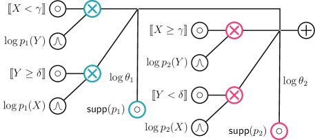
Figure 3: Building the logarithmic circuit (right) for a deterministic PC (left) whose input units are labeled by their supports. A single sum unit is introduced over smoothed product units and additional dummy input units which share the same support across circuits if they have the same color.

Breaking the logarithm over deterministic sum units follows the same idea of the restricted power and is detailed by Thm. B.11. Ultimately, we can merge the sum units coming from the logarithm of products into a single sum to obtain a polysize circuit (Alg. 7). Fig. 3 illustrates this process for a small PC. Note that constructing a logarithm circuit in such a way would compromise determinism for the sum unit $s$, as multiple of its newly introduced inputs would be non-zero for a single configuration $\boldsymbol{x}$. Nevertheless, these inputs of $s$ can be clearly partitioned into groups sharing the same support of the original product unit ${p}$, as illustrated in Fig. 3. This implies that whenever we have to multiply a deterministic circuit and its logarithmic circuit—for instance to compute its entropy (Sec. 4)—we can leverage the sparsifying effect of non-overlapping supports and perform only a linear number of products (Sec. 3.4).

3.6 Exponentials of a Circuit

The exponential of a circuit ${p}(\mathbf{X})$, i.e., $\exp({p}(\mathbf{X}))$, is the inverse operation of the logarithm and is a fundamental operation when representing distributions such as log-linear models (Koller & Friedman, 2009). Similarly to the logarithm, building a decomposable circuit that encodes an exponential of a circuit is #P-hard in general (Thm. B.12). Unlike the logarithm however, restricting the operation to deterministic circuits does not help with tractability, since the issue comes from product units: the exponential of a product is neither a sum nor product of exponentials.

Nevertheless, if ${p}$ encodes a linear sum over its variables, i.e., ${p}(\mathbf{X})=\sum_{i}\theta_{i}X_{i}$, we could easily represent its exponential as a circuit comprising a single decomposable product unit (Prop. B.2). If we were to add an additional deterministic sum unit over many omni-compatible circuits built in such a way, we would retrieve a mixture of truncated exponential model (Moral et al., 2001; Zeng et al., 2020). This is the largest class of tractable exponentials we know so far. Enlarging its boundaries is an interesting open problem.

4 …to Complex Compositional Queries

In this section, we show how our atlas of simple tractable operators can be effectively used to characterize several advanced queries, generalizing existing results in the literature and charting the tractability boundaries for novel ones.

Table 2: Tractability and hardness of information-theoretic queries over circuits. Tractability given some conditions over the input circuits; computational hardness without some of these input condition.

Query		Tractability Conditions		Hardness
Cross Entropy	$-{\color[rgb]{0.15625,0.15625,0.15625}\int}{p}(\boldsymbol{x})\log{q}(\boldsymbol{x})$ d$\mathbf{X}$	Cmp, ${q}$ Det	(Thm. C.2)	#P-hard w/o Det	(Thm. C.1)
Shannon Entropy	$-{\color[rgb]{0.15625,0.15625,0.15625}\sum}{p}(\boldsymbol{x})\log{p}(\boldsymbol{x})$	Sm, Dec, Det	(Thm. C.4)	coNP-hard w/o Det	(Thm. C.3)
Rényi Entropy	$(1-\alpha)^{-1}\log{\color[rgb]{0.15625,0.15625,0.15625}\int}{p}^{\alpha}(\boldsymbol{x})\>d\mathbf{X},\alpha\in\mathbb{N}$	SD	(Thm. C.11)	#P-hard w/o SD	(Thm. C.9)
	$(1-\alpha)^{-1}\log{\color[rgb]{0.15625,0.15625,0.15625}\int}{p}^{\alpha}(\boldsymbol{x})\>d\mathbf{X},\alpha\in\mathbb{R}_{+}$	Sm, Dec, Det	(Thm. C.12)	#P-hard w/o Det	(Thm. C.10)
Mutual Information	${\color[rgb]{0.15625,0.15625,0.15625}\int}p(\boldsymbol{x},\boldsymbol{y})\log(p(\boldsymbol{x},\boldsymbol{y})/(p(\boldsymbol{x})p(\boldsymbol{y})))$	Sm, SD, DetFootnote 4	(Thm. C.6)	coNP-Hard w/o SD	(Thm. C.5)
Kullback-Leibler Div.	${\color[rgb]{0.15625,0.15625,0.15625}\int}{p}(\boldsymbol{x})\log({p}(\boldsymbol{x})/{q}(\boldsymbol{x}))d\mathbf{X}$	Cmp, Det	(Thm. C.8)	#P-hard w/o Det	(Thm. C.7)
Rényi’s Alpha Div.	$(1-\alpha)^{-1}\log{\color[rgb]{0.15625,0.15625,0.15625}\int}{p}^{\alpha}(\boldsymbol{x}){q}^{1-\alpha}(\boldsymbol{x})\>d\mathbf{X},\alpha\in\mathbb{N}$	Cmp, ${q}$ Det	(Thm. C.14)	#P-Hard w/o Det	(Thm. C.13)
	$(1-\alpha)^{-1}\log{\color[rgb]{0.15625,0.15625,0.15625}\int}{p}^{\alpha}(\boldsymbol{x}){q}^{1-\alpha}(\boldsymbol{x})\>d\mathbf{X},\alpha\in\mathbb{R}$	Cmp, Det	(Thm. C.14)	#P-Hard w/o Det	(Thm. C.13)
Itakura-Saito Div.	${\color[rgb]{0.15625,0.15625,0.15625}\int}[{p}(\boldsymbol{x})/{q}(\boldsymbol{x})-\log({p}(\boldsymbol{x})/{q}(\boldsymbol{x}))-1]d\>\mathbf{X}$	Cmp, Det	(Thm. C.16)	#P-Hard w/o Det	(Thm. C.15)
Cauchy-Schwarz Div.	$-\log\frac{{\color[rgb]{0.15625,0.15625,0.15625}\int}{p}(\boldsymbol{x}){q}(\boldsymbol{x})d\mathbf{X}}{\sqrt{{\color[rgb]{0.15625,0.15625,0.15625}\int}{p}^{2}(\boldsymbol{x})d\mathbf{X}{\color[rgb]{0.15625,0.15625,0.15625}\int}{q}^{2}(\boldsymbol{x})d\mathbf{X}}}$	Cmp	(Thm. C.18)	#P-Hard w/o Cmp	(Thm. C.17)
Squared loss	${\color[rgb]{0.15625,0.15625,0.15625}\int}{({p}(\boldsymbol{x})-{q}(\boldsymbol{x}))^{2}}d\>\mathbf{X}$	Cmp	(Thm. C.20)	#P-Hard w/o Cmp	(Thm. C.19)

Given a complex query over one or more input models that involves a pipeline of operations culminating in an integration (Fig. 1), we can quickly devise a tractable model class for it by inferring the sufficient conditions needed for tractably computing each operation—starting from the last one and propagating them backwards according to Tab. 1. Consider the example of computing the KLD between two distributions $p$ and $q$ mentioned in Sec. 1. To compute integration we require a smooth and decomposable circuit (Prop. 2.1). Therefore, the two circuits that participate in the product, i.e., $p$ and $\log(p/q)$, should be compatible (Thm. B.2). Thm. B.11 tells us that the logarithm of a circuit can be tractably computed when restricted over the support of a deterministic input circuit. Moreover, the logarithm of a structured-decomposable circuit is going to retain this property and be compatible with its input. Therefore, we require the quotient $p/q$ to be deterministic and compatible with $p$. We know this can be obtained if both $p$ and $q$ are deterministic and compatible (Thm. B.9). As such, we can conclude that for two deterministic and compatible PCs $p$ and $q$ we can compute their tractable KLD (Thm. C.8). In the following, we summarize analogous derivations for many different queries, as detailed in Tab. 2, for which we report also novel complexity results to complete our theoretical understanding of these operations.

Theorem 4.1.

The tractability and hardness results for complex queries as reported in Tab. 2 hold.

Shannon entropy Recall from Sec. 2.1 that many classical tractable models are special cases of PCs with certain structural properties. As such, all the results for general circuits will translate over these model classes. For instance, we can tractably compute the Shannon entropy for bounded-treewidth PGMs such as Chow-Liu trees and polytrees, as they can be represented as smooth, decomposable and deterministic PCs (Thm. C.4). This is possible because multiplying a circuit ${p}$ with its logarithm $\log{p}$ can be done in linear time as the latter will share its support structure (Sec. 3.5). Moreover, we demonstrate in Thm. C.3 that computing the Shannon entropy is coNP-hard for non-deterministic PCs. This closes an open question recently raised by Shih & Ermon (2020), where a linear time algorithm for selective sum-product networks, a special case of deterministic and decomposable PCs, was introduced.

Rényi entropy For non-deterministic PCs we can employ the tractable computation of Rényi entropy of order $\alpha$ (Rényi et al., 1961), which recovers Shannon Entropy for $\alpha\rightarrow 1$. As the logarithm is taken after integration of the power circuit, the tractability and hardness follow directly from those of the power operation.

Cross entropy As hinted by the presence of logarithm, the cross entropy is #P-hard to compute without determinism, even for compatible PCs (Thm. C.1). Nevertheless, we can derive the conditions for tractability using our vocabulary of simple operations. As it shares some sub-operations with the KLD (Fig. 1), the cross entropy can be tractably computed in $\mathcal{O}(\left\lvert{p}\right\rvert\left\lvert{q}\right\rvert)$ if ${p}$ and ${q}$ are deterministic and compatible.

Mutual information Building on these insights, we characterize the tractability of mutual information (MI) between sets of variables $\mathbf{X}$ and $\mathbf{Y}$ w.r.t. their joint distribution ${p}(\mathbf{X},\mathbf{Y})$ encoded as a PC. Let the marginals ${p}(\mathbf{X})$ and ${p}(\mathbf{Y})$ be represented as PCs as well, which can be done in linear time for smooth and decomposable PCs (Choi et al., 2020). Then the MI over these three PCs can be computed via a pipeline involving product, quotient, and log operators. From Tab. 1, we can infer that the MI is tractable if all circuits are compatible and deterministic. For non-deterministic PCs we prove it to be coNP-Hard (Thm. C.5).

Divergences Liang & Van den Broeck (2017) proposed an efficient algorithm to compute the KLD tailored for PSDDs. This has been the only tractable divergence available for PCs so far. We greatly extend this panorama by listing other tractable divergences employing the simple operations studied so far, and additionally proving their hardness for missing structural properties over their inputs.

Rényi’s $\alpha$-divergences (Rényi et al., 1961) generalize several divergences such as the KLD when $\alpha\!\rightarrow\!1$, Hellinger’s squared divergence when $\alpha\!=\!2^{-1}$, and the $\mathcal{X}^{2}$-divergence when $\alpha\!=\!2$ (Gibbs & Su, 2002). They are tractable for compatible and deterministic PCs, as is the Itakura-Saito divergence which has applications in learning and signal processing (Wei & Gibson, 2001).

For non-deterministic PCs, we list the squared loss and the Cauchy-Schwarz divergence (Jenssen et al., 2006). The latter has applications in mixture models for approximate inference (Tran et al., 2021) and has been derived in closed-form for mixtures of simple parametric forms like Gaussians (Kampa et al., 2011), Weibull and Rayligh distributions (Nielsen, 2012). Our results generalize them to deep mixture models (Poon & Domingos, 2011).

Expectation queries Among other complex queries that can be abstracted into the general form of an expectation of a circuit $f$ w.r.t. a PC ${p}$, i.e., $\mathbb{E}_{\boldsymbol{x}\sim{p}(\mathbf{X})}\left[f(\boldsymbol{x})\right]$, there are the moments of distributions, such as means and variances. They can be efficiently computed for any smooth and decomposable PC, as $f$ is an omni-compatible circuit (Prop. D.1). This result generalizes the moment computation for simple models such as GMMs and HMMs as they can be encoded as smooth and decomposable PCs (Sec. 2.1).

If $f$ is the indicator function of a logical formula, the expectation computes its probability w.r.t. the distribution ${p}$. Choi et al. (2015) proposed an algorithm tailored to formulas $f$ over binary variables, encoded as SDDs (Darwiche, 2011) w.r.t. distributions that are PSDDs. We generalize this result to mixed continuous-discrete distributions encoded as structured-decomposable PCs that are not necessarily deterministic and to logical formulas in the language of satisfiability modulo theories (Barrett & Tinelli, 2018) over linear arithmetics with univariate literals (Prop. D.2). Lastly, if $f$ encodes constraints over the output distribution of a deep network we retrieve the semantic loss (Xu et al., 2018).

If $f$ encodes a classifier or a regressor, then $\mathbb{E}_{p}[f]$ refers to computing its expected predictions w.r.t. $p$ (Khosravi et al., 2019b). Our results generalize computing the expectations of decision trees and their ensembles as proposed by Khosravi et al. (2020) (cf. Prop. D.3) as well as those of deep regression circuits (Khosravi et al., 2019a).

5 Discussion and conclusions

In this work we introduced a unified framework to reason about tractable model classes w.r.t. many queries common in probabilistic ML and AI. Tractability is studied by rewriting complex queries as combinations of simpler operations and pushing sufficient conditions through the latter, leading to a rich atlas that can guide and inspire future research.

The most closely related work resides in the literature of logical circuits, which encode Boolean functions as computational graphs with AND and OR gates. Structural properties analogous to those we introduced for circuits (Sec. 2.1) can be defined for logical circuits (Darwiche & Marquis, 2002) and deterministic logical circuits can be directly translated as circuits with sums and products instead of OR and AND gates. Tractable logical circuit operations such as disjunctions and conjunctions—the analogous to our (deterministic) sum and products—have been investigated for several logical formalisms (Darwiche & Marquis, 2002). Our results generalize the Boolean case for these operations. We also introduce novel operations, including powers and logarithms as well as complex queries such as divergences, that have no direct counterpart in the logical domain.

Algorithms to tractably multiply two probabilistic models have been proposed in the context of probabilistic decision graphs (PDGs) (Jaeger, 2004; Jaeger et al., 2006) first and PSDDs later (Shen et al., 2016). Despite the different syntax, both PDGs and PSDDs can be represented as structured-decomposable and deterministic circuits in our language (Choi et al., 2020). Differently from our treatment in Sec. 2.1, PDGs and PSDDs define compatibility in terms of special notions of hierarchical scope partitioning, namely pseudo forests (Jaeger, 2004) and vtrees (Pipatsrisawat & Darwiche, 2008), respectively. In particular, they differ from our general characterization in that they (1) enforce a positional ordering over the partitions and (2) imbue this ordering with the semantic of conditioning over one set of variables to obtain the distribution over the others. As such, these representations entangle determinism and compatibility. As we showed in Thm. B.2, compatibility is sufficient for tractable multiplication, and as discussed in the previous section many algorithms tailored for PSDDs (Choi et al., 2015; Shen et al., 2016; Khosravi et al., 2019a) can be generalized to non-deterministic distributions in our framework.

Our property-driven analysis closes many open questions about the tractability and hardness of queries for many model classes that are special cases of circuits. Nevertheless, other interesting questions remain open and constitute possible future directions. For instance, demonstrating unconditional lower bounds for our representations or extending our analysis to queries involving maximization—that is, MAP inference over probability distributions. On the other hand, our atlas could support the design of learning routines for circuits in different ways. First, existing algorithms (Rahman et al., 2014; Vergari et al., 2015; Peharz et al., 2019; Dang et al., 2020) could be enriched by our new transformations to generate tractable structures. Second, our analysis could help design novel algorithms to learn circuits that are tailored to answer multiple queries efficiently at once, in a sort of multi-objective optimization scenario where the algorithm trades-off circuit sizes across different queries.

Io so. Ma non ho le prove.

Appendix A Useful Sub-Routines

This section introduces the algorithmic construction of gadget circuits that will be adopted in our proofs of tractability as well as hardness. We start by introducing three primitive functions for constructing circuits—Input, Sum, and Product.

$\bullet$ $\textsc{Input}(l_{p},\phi({p}))$ constructs an input unit that encodes a parameterized function $l_{p}$ over variables $\phi({p})$. For example, $\textsc{Input}(\llbracket{X=\mathrm{True}}\rrbracket,X)$ and $\textsc{Input}(\llbracket{X=\mathrm{False}}\rrbracket,X)$ represent the positive and negative literals of a Boolean variable $X$, respectively. On the other hand, $\textsc{Input}(\mathcal{N}(\mu,\sigma),X)$ defines a Gaussian pdf with mean $\mu$ and standard deviation $\sigma$ as an input function.

$\bullet$ $\textsc{Sum}(\{{p}_{i}\}_{i=1}^{k},\{\theta_{i}\}_{i=1}^{k})$ constructs a sum unit that represents the weighted combination of circuit units $\{{p}_{i}\}_{i=1}^{k}$ encoded as an ordered set w.r.t. the correspondingly ordered weights $\{\theta_{i}\}_{i=1}^{k}$.

$\bullet$ $\textsc{Product}(\{{p}_{i}\}_{i=1}^{k})$ builds a product unit that encodes the product of circuit units $\{{p}_{i}\}_{i=1}^{k}$.

A.1 Support circuit of a deterministic circuit

Algorithm 1 Support(${p},\mathsf{cache}$)

1:  Input: a smooth, deterministic, and decomposable circuit ${p}$ over variables $\mathbf{X}$ and a cache for memorization

2:  Output: a smooth, deterministic, and decomposable circuit $s$ over $\mathbf{X}$ encoding $s(\boldsymbol{x})=\llbracket{\boldsymbol{x}\in\mathsf{supp}({p})}\rrbracket$

3:  if ${p}\in\mathsf{cache}$ then return $\mathsf{cache}({p})$

4:  if ${p}$ is an input unit then

5:     $s\leftarrow\textsc{Input}(\llbracket{\boldsymbol{x}\in\mathsf{supp}({p})}\rrbracket,{\phi}(p))$

6:  else if ${p}$ is a sum unit then

7:     $s\leftarrow\textsc{Sum}(\{\textsc{Support}({p}_{i},\mathsf{cache})\}_{i=1}^{|\mathsf{in}({p})|},\{1\}_{i=1}^{|\mathsf{in}({p})|})$

8:  else if ${p}$ is a product unit then

9:     $s\leftarrow\textsc{Product}(\{\textsc{Support}({p}_{i},\mathsf{cache})\}_{i=1}^{|\mathsf{in}({p})|}|)$

10:  $\mathsf{cache}({p})\leftarrow s$

11:  return $s$

Given a smooth, decomposable, and deterministic circuit ${p}(\mathbf{X})$, its support circuit $s(\mathbf{X})$ is a smooth, decomposable, and deterministic circuit that evaluates $1$ iff the input $\boldsymbol{x}$ is in the support of ${p}$ (i.e., $\boldsymbol{x}\in\mathsf{supp}({p})$) and otherwise evaluates $0$, as defined below.

Definition A.1 (Support circuit).

Let ${p}$ be a smooth, decomposable, and deterministic PC over variables $\mathbf{X}$. Its support circuit is the circuit $s$ that computes $s(\boldsymbol{x})=\llbracket{\boldsymbol{x}\in\mathsf{supp}(p)}\rrbracket$, obtained by replacing every sum parameter of ${p}$ by 1 and every input distribution $l$ by the function $\llbracket{\boldsymbol{x}\in\mathsf{supp}(l)}\rrbracket$.

A construction algorithm for the support circuit is provided in Alg. 1. This algorithm will later be useful in defining some circuit operations such as the logarithm.

A.2 Circuits encoding uniform distributions

We can build a deterministic and omni-compatible PC that encodes a (possibly unnormalized) uniform distribution over binary variables $\mathbf{X}=\{X_{1},\ldots,X_{n}\}$: i.e., $p(\boldsymbol{x})=c$ for a constant $c\in\mathbb{R}_{+}$ for all $\boldsymbol{x}\in\mathsf{val}(\mathbf{X})$. Specifically, ${p}$ can be defined as a single sum unit with weight $c$ that receives input from a product unit over $n$ univariate input distribution units that always output 1 for all values $\mathsf{val}(X_{i})$. This construction is summarized in Alg. 2. It is a key component in the algorithms for many tractable circuit transformations/queries as well as in several hardness proofs.

Algorithm 2 uniformCircuit($\mathbf{X},c$)

1:  Input: a set of variables $\mathbf{X}$ and constant $c\in\mathbb{R}_{+}$.

2:  Output: a deterministic and omni-compatible PC encoding an unnormalized uniform distribution over $\mathbf{X}$.

3:  $n\leftarrow\{\}$

4:  for $i=1$ to $|\mathbf{X}|$ do

5:     $m\leftarrow\{\}$

6:     for $x_{i}$ in $\mathsf{val}(X_{i})$ do

7:        $m\leftarrow m\cup\{\textsc{Input}(\llbracket{X_{i}=x_{i}}\rrbracket,X_{i})\}$

8:     $n\leftarrow n\cup\{\textsc{Sum}(m,\{1\}_{j=1}^{|\mathsf{val}(X_{i})|})\}$

9:  return $\textsc{Sum}(\{\textsc{Product}(n)\},\{c\})$

A.3 A circuit representation of the #3SAT problem

We define a circuit representation of the #3SAT problem, following the construction in Khosravi et al. (2019a). Specifically, we represent each instance in the #3SAT problem as two poly-sized structured-decomposable and deterministic circuits ${p}_{\beta}$ and ${p}_{\gamma}$, such that the partition function of their product equals the solution of the original #3SAT problem.

#3SAT is defined as follows: given a set of $n$ boolean variables $\mathbf{X}=\{X_{1},\dots,X_{n}\}$ and a CNF that contains $m$ clauses $\{c_{1},\dots,c_{m}\}$ (each clause contains exactly 3 literals), count the number of satisfiable worlds in $\mathsf{val}(\mathbf{X})$.

For every variable $X_{i}$ in clause $c_{j}$, we introduce an auxiliary variable $X_{ij}$. Intuitively, $\{X_{ij}\}_{j=1}^{m}$ are copies of the variable $X_{i}$, one for each clause. Therefore, for any $i$, $\{X_{ij}\}_{j=1}^{m}$ share the same value (i.e., true or false), which can be represented by the following formula $\beta$:

$$\beta\equiv\bigwedge\limits_{i=1}^{n}(X_{i1}\Leftrightarrow X_{i2}\Leftrightarrow\cdots\Leftrightarrow X_{im}).$$

Then we can encode the original CNF in the following formula $\gamma$ by substituting $X_{i}$ with the respective $X_{ij}$ in each clause:

$$\gamma\equiv\bigwedge\limits_{j=1}^{m}\bigvee\limits_{i:X_{i}\in\phi(c_{j})}l(X_{ij}),$$

where $\phi(c)$ denotes the variable scope of clause $c$, and $l(X_{ij})$ denotes the literal of $X_{i}$ in clause $c_{j}$. Since $\beta$ restricts the variables $\{X_{ij}\}_{j=1}^{m}$ to have the same value, the model count of $\beta\wedge\gamma$ is equal to the model count of the original CNF.

We are left to show that both $\beta$ and $\gamma$ can be compiled into a poly-sized structured-decomposable and deterministic circuit. We start from compiling $\beta$ into a circuit ${p}_{\beta}$. Note that for each $i$, $(X_{i1}\Leftrightarrow\cdots\Leftrightarrow X_{im})$ has exactly two satisfiable variable assigments (i.e., all true or all false), it can be compiled as a sum unit $a_{i}$ over two product units $b_{i1}$ and $b_{i2}$ (both weights of $a$ are set to $1$), where $b_{i1}$ takes inputs from the positive literals $\{X_{i1},\dots,X_{im}\}$ and $b_{i2}$ from the negative literals $\{\neg X_{i1},\dots,\neg X_{im}\}$. Then ${p}_{\beta}$ is represented by a product unit over $\{a_{1},\dots,a_{n}\}$. Note that by definition this ${p}_{\beta}$ circuit is structured-decomposable and deterministic.

We proceed to compile $\gamma$ into a polysized structured-decomposable and deterministic circuit ${p}_{\gamma}$. Note that in #3SAT, each clause $c_{j}$ contains 3 literals. Therefore, for any $j\in\{1,\dots,m\}$, $\bigvee_{X_{i}\in\phi(c_{j})}l(X_{ij})$ has exactly 7 models w.r.t. the variable scope $\phi(c_{j})$. Hence, we compile $\bigvee_{X_{i}\in\phi(c_{j})}l(X_{ij})$ into a circuit $d_{j}$, which is a sum unit with 7 inputs $\{e_{j1},\dots,e_{j7}\}$. Each $e_{jh}$ is constructed as a product unit over variables $\{X_{1j},\dots,X_{nj}\}$ that represents the $h$-th model of clause $c_{j}$. More formally, we have $e_{jh}\leftarrow\textsc{Product}(\{g_{ijh}\}_{i=1}^{n})$, where $g_{ijh}$ is a sum unit over literals $X_{ij}$ and $\neg X_{ij}$ (with both weights being $1$) if $i\not\in\phi(c_{j})$ and otherwise $g_{ijh}$ is the literal unit corresponds to the $h$-th model of clause $c_{j}$. The circuit ${p}_{\gamma}$ representing the formula $\gamma$ is constructed by a product unit with inputs $\{d_{j}\}_{j=1}^{m}$. By construction this circuit is also structured-decomposable and deterministic.

Appendix B Circuit Operations

This section formally presents the tractability and hardness results w.r.t. circuit operations summarized in Tab. 1—sums, products, quotients, powers, logarithms, and exponentials. For each circuit operation, we provide both its proof of tractability by constructing a polytime algorithm given sufficient structural constraints and novel hardness results that identify necessary structural constraints for the operation to yield a decomposable circuit as output.

Throughout this paper, we will show hardness of operations to output a decomposable circuit by proving hardness of computing the partition function of the output of the operation. This follows from the fact that we can smooth and integrate a decomposable circuit in polytime, thereby making the former problem at least as hard as the latter.

For the tractability theorems, we will assume that the operation referenced by the theorem is tractable over input units of circuit or pairs of compatible input units whose element belong each to a circuit. For example, for Thm. B.2 we assume tractable product of input units sharing the same scope and for Thm. B.6 we assume that the powers of the input units can be tractably represented as a single new unit.

Moreover, in the following results, we will adopt a more general definition of compatibility that can be applied to circuits with different variable scopes, which is often useful in practice. Formally, consider two circuits ${p}$ and ${q}$ with variable scope $\mathbf{Z}$ and $\mathbf{Y}$. Analogous to Def. 2.5, we say that ${p}$ and ${q}$ are compatible over variables $\mathbf{X}=\mathbf{Z}\cap\mathbf{Y}$ if (1) they are smooth and decomposable and (2) any pair of product units $n\in{p}$ and $m\in{q}$ with the same overlapping scope with $\mathbf{X}$ can be rearranged into mutually compatible binary products. Note that since our tractability results hold for this extended definition of compatibility, they are also satisfied under Def. 2.5.

B.1 Sum of Circuits

The hardness of the sum of two circuits to yield a deterministic circuit has been proven by Shen et al. (2016) in the context of arithmetic circuits (ACs) (Darwiche & Marquis, 2002). ACs can be readily turned into circuits over binary variables according to our definition by translating their input parameters into sum parameters as done in Rooshenas & Lowd (2014).

A sum of circuits will preserve decomposability and related properties as the next proposition details.

Proposition B.1 (Closure of sum of circuits).

Let ${p}(\mathbf{Z})$ and ${q}(\mathbf{Y})$ be decomposable circuits. Then their sum circuit $s(\mathbf{Z}\cup\mathbf{Y})=\theta_{1}\cdot{p}(\mathbf{Z})+\theta_{2}\cdot{q}(\mathbf{Y})$ for two reals $\theta_{1},\theta_{2}\in\mathbb{R}$ is decomposable. If ${p}$ and ${q}$ are structured-decomposable and compatible, then $s$ is structured-decomposable and compatible with both ${p}$ and ${q}$. Lastly, if both inputs are also smooth, $s$ can be smoothed in polytime.

Proof.

If ${p}$ and ${q}$ are decomposable, $s$ is also decomposable by definition (no new product unit is introduced). If they are also structured-decomposable and compatible, $s$ would be structured-decomposable and compatible with ${p}$ and ${q}$ as well, as summation does not affect their hierarchical scope partitioning. Note that if one input is decomposable and the other omni-compatible, then $s$ would only be decomposable.

If $\mathbf{Z}=\mathbf{Y}$ then $s$ would be smooth; otherwise we can smooth it in polytime (Darwiche, 2009; Shih et al., 2019), i.e., by realizing the circuit

$$s(\boldsymbol{x})= \;\theta_{1}\cdot{p}(\boldsymbol{z})\cdot\llbracket{{q}(\left.{\boldsymbol{x}}\right\rvert_{\mathbf{Y}\setminus\mathbf{Z}})\neq 0}\rrbracket+$$

$$\;\theta_{2}\cdot{q}(\boldsymbol{y})\cdot\llbracket{{p}(\left.{\boldsymbol{x}}\right\rvert_{\mathbf{Z}\setminus\mathbf{Y}})\neq 0}\rrbracket$$

where $\llbracket{{q}(\left.{\boldsymbol{x}}\right\rvert_{\mathbf{Y}\setminus\mathbf{Z}})\neq 0}\rrbracket$ (resp. $\llbracket{{p}(\left.{\boldsymbol{x}}\right\rvert_{\mathbf{Z}\setminus\mathbf{Y}})\neq 0}\rrbracket$ ) can be encoded as an input distribution over variables $\mathbf{Y}\setminus\mathbf{Z}$ (resp.$\mathbf{Z}\setminus\mathbf{Y}$). Note that if the supports of ${p}(\mathbf{Z}\setminus\mathbf{Y})$ and ${q}(\mathbf{Y}\setminus\mathbf{Z})$ are not bounded, then integrals over them would be unbounded as well. ∎

B.2 Product of Circuits

Theorem B.1 (Hardness of product of circuits).

Let ${p}$ and ${q}$ be two structured-decomposable and deterministic circuits over variables $\mathbf{X}$. Computing their product $m(\mathbf{X})={p}(\mathbf{X})\cdot{q}(\mathbf{X})$ as a decomposable circuit is #P-Hard.

Proof.

As noted earlier, we will prove hardness of computing the product by showing hardness of computing the partition function of a product of two circuits. In particular, let ${p}$ and ${q}$ be two structured-decomposable and deterministic circuits over binary variables $\mathbf{X}$. Then, computing the following quantity is #P-hard:

$$\sum_{\boldsymbol{x}\in\mathsf{val}(\mathbf{X})}{p}(\boldsymbol{x})\cdot{q}(\boldsymbol{x}).$$ (MULPC)

The following proof is adapted from the proof of Thm. 2 in Khosravi et al. (2019a). We reduce the #3SAT problem defined in Sec. A.3, which is known to be #P-hard, to MULPC. Recall that ${p}_{\beta}$ and ${p}_{\gamma}$, as constructed in Sec. A.3, are structured-decomposable and deterministic; additionally, the partition function of ${p}_{\beta}\cdot{p}_{\gamma}$ is the solution of the corresponding #3SAT problem. In other words, computing MULPC of two structured-decomposable and deterministic circuits ${p}_{\beta}$ and ${p}_{\gamma}$ exactly solves the original #3SAT problem. Therefore, computing the product of two structured-decomposable and deterministic circuits is #P-Hard. ∎

Theorem B.2 (Tractable product of circuits).

Let ${p}(\mathbf{Z})$ and ${q}(\mathbf{Y})$ be two compatible circuits over variables $\mathbf{X}=\mathbf{Z}\cap\mathbf{Y}$. Then, computing their product ${m}(\mathbf{X})={p}(\mathbf{Z})\cdot{q}(\mathbf{Y})$ as a decomposable circuit can be done in $\mathcal{O}(\left\lvert{p}\right\rvert\left\lvert{q}\right\rvert)$ time and space. If both ${p}$ and ${q}$ are also deterministic, then so is ${m}$, moreover if ${p}$ and ${q}$ are structured-decomposable then ${m}$ is compatible with ${p}$ (and ${q}$) over $\mathbf{X}$.

Proof.

The proof proceeds by showing that computing the product of (i) two smooth and compatible sum units ${p}$ and ${q}$ and (ii) two smooth and compatible product units ${p}$ and ${q}$ given the product circuits w.r.t. pairs of child units from ${p}$ and ${q}$ (i.e., $\forall r\in\mathsf{in}({p})\,s\in\mathsf{in}({q}),(r\!\cdot\!s)(\mathbf{X})$) takes time $\mathcal{O}(\left\lvert\mathsf{in}({p})\right\rvert\left\lvert\mathsf{in}({q})\right\rvert)$. Then, by recursion, the overall complexity in time and space are both $\mathcal{O}(\left\lvert{p}\right\rvert\left\lvert{q}\right\rvert)$. Alg. 3 illustrates the overall process in detail.

If ${p}$ and ${q}$ are two sum units defined as ${p}(\boldsymbol{x})=\sum_{i\in\mathsf{in}({p})}\theta_{i}{p}_{i}(\boldsymbol{x})$ and ${q}(\boldsymbol{x})=\sum_{j\in\mathsf{in}({q})}\theta^{\prime}_{j}{q}_{j}(\boldsymbol{x})$, respectively. Then, their product $m(\boldsymbol{x})$ can be broken down to the weighted sum of $\left\lvert\mathsf{in}({p})\right\rvert\!\cdot\!\left\lvert\mathsf{in}({q})\right\rvert$ circuits that represent the products of pairs of their inputs:

$$m(\boldsymbol{x}) =\left(\sum_{i\in\mathsf{in}({p})}\theta_{i}{p}_{i}(\boldsymbol{x})\right)\left(\sum_{j\in\mathsf{in}({q})}\theta^{\prime}_{j}{q}_{j}(\boldsymbol{x})\right)$$

$$= \sum_{i\in\mathsf{in}({p})}\sum_{j\in\mathsf{in}({q})}\theta_{i}\theta^{\prime}_{j}({p}_{i}{q}_{j})(\boldsymbol{x}).$$

Note that this Cartesian product of units is a deterministic sum unit if both ${p}$ and ${q}$ were deterministic sum units, as $\mathsf{supp}({p}_{i}{q}_{j})\!=\!\mathsf{supp}({p}_{i})\cap\mathsf{supp}({q}_{j})$ are disjoint for different $i,j$.

If ${p}$ and ${q}$ are two product units defined as ${p}(\mathbf{X})={p}_{1}(\mathbf{X}_{1}){p}_{2}(\mathbf{X}_{2})$ and ${q}(\mathbf{X})={q}_{1}(\mathbf{X}_{1}){q}_{2}(\mathbf{X}_{2})$, respectively. Then, their product $m(\boldsymbol{x})$ can be constructed recursively from the product of their inputs:

$$m(\boldsymbol{x}) ={p}_{1}(\boldsymbol{x}_{1}){p}_{2}(\boldsymbol{x}_{2})\cdot{q}_{1}(\boldsymbol{x}_{1}){q}_{2}(\boldsymbol{x}_{2})$$

$$={p}_{1}(\boldsymbol{x}_{1}){q}_{1}(\boldsymbol{x}_{1})\cdot{p}_{2}(\boldsymbol{x}_{2}){q}_{2}(\boldsymbol{x}_{2})$$

$$=({p}_{1}{q}_{1})(\boldsymbol{x}_{1})\cdot({p}_{2}{q}_{2})(\boldsymbol{x}_{2}).$$

Note that by this construction ${m}$ retains the same scope partitioning of ${p}$ and ${q}$, hence if they were structured-decomposable, ${m}$ will be structured-decomposable and compatible with ${p}$ and ${q}$. ∎

Algorithm 3 multiply(${p},{q},\mathsf{cache}$)

1:  Input: two circuits ${p}(\mathbf{Z})$ and ${q}(\mathbf{Y})$ that are compatible over $\mathbf{X}=\mathbf{Z}\cap\mathbf{Y}$ and a cache for memoization

2:  Output: their product circuit ${m}(\mathbf{Z}\cup\mathbf{Y})={p}(\mathbf{Z}){q}(\mathbf{Y})$

3:  if $({p},{q})\in\mathsf{cache}$ then return $\mathsf{cache}({p},{q})$

4:  if ${\phi}({p})\cap{\phi}({q})=\emptyset$ then

5:     ${m}\leftarrow\textsc{Product}(\{{p},{q}\});\;s\leftarrow\mathrm{True}$

6:  else if ${p},{q}$ are input units then

7:     ${m}\leftarrow\textsc{Input}({p}(\mathbf{Z})\cdot{q}(\mathbf{Y}),\mathbf{Z}\cup\mathbf{Y})$

8:     $s\leftarrow\llbracket{\mathsf{supp}({p}(\mathbf{X}))\cap\mathsf{supp}({q}(\mathbf{X}))\neq\emptyset}\rrbracket$

9:  else if ${p}$ is an input unit then

10:     ${n}\leftarrow\{\};s\leftarrow\mathrm{False}$ $//{q}(\mathbf{Y})=\sum_{j}\theta^{\prime}_{j}{q}_{j}(\mathbf{Y})$

11:     for $j=1$ to $|\mathsf{in}({q})|$ do

12:        ${n}^{\prime},s^{\prime}\leftarrow\text{{multiply}}({p},{q}_{j},\mathsf{cache})$

13:        ${n}\leftarrow{n}\cup\{{n}^{\prime}\};\;s\leftarrow s\lor s^{\prime}$

14:     if $s$ then ${m}\leftarrow\textsc{Sum}({n},\{\theta^{\prime}_{j}\}_{j=1}^{|\mathsf{in}({q})|})$ else ${m}\leftarrow null$

15:  else if ${q}$ is an input unit then

16:     ${n}\leftarrow\{\};s\leftarrow\mathrm{False}$ $//{p}(\mathbf{Z})=\sum_{i}\theta_{i}{p}_{i}(\mathbf{Z})$

17:     for $i=1$ to $|\mathsf{in}({p})|$ do

18:        ${n}^{\prime},s^{\prime}\leftarrow\text{{multiply}}({p}_{i},{q},\mathsf{cache})$

19:        ${n}\leftarrow{n}\cup\{{n}^{\prime}\};\;s\leftarrow s\lor s^{\prime}$

20:     if $s$ then ${m}\leftarrow\textsc{Sum}({n},\{\theta_{i}\}_{i=1}^{|\mathsf{in}({p})|})$ else ${m}\leftarrow null$

21:  else if ${p},{q}$ are product units then

22:     ${n}\leftarrow\{\};s\leftarrow\mathrm{True}$

23:     $\{{p}_{i},{q}_{i}\}_{i=1}^{k}\leftarrow\mathsf{sortPairsByScope}({p},{q},\mathbf{X})$

24:     for $i=1$ to $k$ do

25:        ${n}^{\prime},s^{\prime}\leftarrow\text{{multiply}}({p}_{i},{q}_{i},\mathsf{cache})$

26:        ${n}\leftarrow{n}\cup\{{n}^{\prime}\};\;s\leftarrow s\land s^{\prime}$

27:     if $s$ then ${m}\leftarrow\textsc{Product}({n})$ else ${m}\leftarrow null$

28:  else if ${p},{q}$ are sum units then

29:     ${n}\leftarrow\{\};\;w\leftarrow\{\};\;s\leftarrow\mathrm{False}$

30:     for $i=1$ to $|\mathsf{in}({p})|$, $j=1$ to $|\mathsf{in}({q})|$ do

31:        ${n}^{\prime},s^{\prime}\leftarrow\text{{multiply}}({p}_{i},{q}_{j},\mathsf{cache})$

32:        ${n}\leftarrow{n}\cup{n}^{\prime};w\leftarrow w\cup\{\theta_{i}\theta^{\prime}_{j}\};s\leftarrow s\lor s^{\prime}$

33:     if $s$ then ${m}\leftarrow\textsc{Sum}({n},w)$ else ${m}\leftarrow null$

34:  $\mathsf{cache}({p},{q})\leftarrow({m},s)$

35:  return ${m},s$

Possessing additional structural constrains can lead to sparser output circuits as well as efficient algorithms to construct them. First, if one among ${p}$ and ${q}$ is omni-compatible, it suffices that the other is just decomposable to obtain a tractable product, whose size this time is going to be linear in the size of the decomposable circuit.

Corollary B.2.1.

Let ${p}$ be a smooth and decomposable circuit over $\mathbf{X}$ and ${q}$ an omni-compatible circuit over $\mathbf{X}$ comprising a sum unit with $k$ inputs, hence its size is $k\left\lvert\mathbf{X}\right\rvert$. Then, ${m}(\mathbf{X})={p}(\mathbf{X}){q}(\mathbf{X})$ is a smooth and decomposable circuit constructed in $\mathcal{O}(k\left\lvert{p}\right\rvert)$ time and space.

Second, if ${p}$ and ${q}$ have inputs with restricted supports, their product is going to be sparse, i.e., only a subset of their inputs is going to yield a circuit that does not constantly output zero. Note that in Alg. 3 we can check in polytime if the supports of two units to be multiplied are overlapping by a depth-first search (realized with a Boolean indicator $s$ in Alg. 3), thanks to decomposability. Therefore, for two compatible sum units $p$ and $q$ we will effectively build a number of units that is

$$\mathcal{O}(\left\lvert\{({p}_{i},{q}_{j})|{p}_{i}\!\in\!\mathsf{in}({p}),{q}_{i}\!\in\!\mathsf{in}({q}),\mathsf{supp}({p}_{i})\!\cap\!\mathsf{supp}({q}_{j})\!\neq\!\emptyset\}\right\rvert).$$

In practice, this sparsifying effect will be more prominent when both ${p}$ and ${q}$ are deterministic. This is because having disjoint supports is required for deterministic circuits. This “decimation” of product units will be maximum if $p$ and $q$ partition the support in the very same way, for instance when we have $p=q$, i.e., we are multiplying one circuit with itself, or we are dealing with a logarithmic circuit (cf. Sec. 3.5). In such a case, we can omit the depth-first check for overlapping supports of the product units participating in the product of a sum unit. If both ${p}$ and ${q}$ have an identifier for their supports, we can simply check for equality of their identifiers. This property and algorithmic insight will be key when computing powers of a deterministic circuit and its entropies (cf. Sec. C.2), as it would suffice the input circuit $p$ to be decomposable (cf. Sec. 3.3) to obtain a linear time complexity.

Algorithm 4 sortPairsByScope(${p},{q},\mathbf{X}$)

1:  Input: two decomposable and compatible product units $p$ and $q$, and a variable scope $\mathbf{X}$.

2:  Output: Pairs of compatible sum units $\{(p_{i},q_{i})\}_{i=1}^{k}$.

3:  $\mathrm{children}\_p\leftarrow\{p_{i}\}_{i=1}^{\left\lvert\mathsf{in}({p})\right\rvert},\quad\mathrm{children}\_q\leftarrow\{q_{i}\}_{i=1}^{\left\lvert\mathsf{in}({q})\right\rvert}$

4:  $\mathrm{pairs}\leftarrow\{\}$. $//$ “$\mathrm{pairs}$” stores circuit pairs with matched scope.

5:  $\mathrm{cmp}\_p\leftarrow\{\{\}\}_{i=1}^{\left\lvert\mathsf{in}({p})\right\rvert},\quad\mathrm{cmp}\_q\leftarrow\{\{\}\}_{j=1}^{\left\lvert\mathsf{in}({q})\right\rvert}$.$//$ $\mathrm{cmp}\_p[i]$ (resp. $\mathrm{cmp}\_q[j]$) stores the children of ${q}$ (resp. ${p}$) whose scopes are subsets of ${p}_{i}$’s (resp. ${q}_{j}$’s) scope.

6:  for i = 1 to $|\mathsf{in}({p})|$ do

7:     for j = 1 to $|\mathsf{in}({q})|$ do

8:        if $\phi({p}_{i})\cap\mathbf{X}=\phi({q}_{j})\cap\mathbf{X}$ then

9:           $\mathrm{pairs}.append(({p}_{i},{q}_{j}))$

10:           $\mathrm{children}\_p.pop({p}_{i}),\quad\mathrm{children}\_q.pop({q}_{j})$

11:        else if $\phi({p}_{i})\cap\mathbf{X}\subset\phi({q}_{j})\cap\mathbf{X}$ then

12:           $\mathrm{cmp}\_q[j].append({p}_{i})$

13:           $\mathrm{children}\_p.pop({p}_{i}),\quad\mathrm{children}\_q.pop({q}_{j})$

14:        else if $\phi({q}_{j})\cap\mathbf{X}\subset\phi({p}_{i})\cap\mathbf{X}$ then

15:           $\mathrm{cmp}\_p[i].append({q}_{j})$

16:           $\mathrm{children}\_p.pop({p}_{i}),\quad\mathrm{children}\_q.pop({q}_{j})$

17:  for $i=1$ to $\left\lvert\mathsf{in}({p})\right\rvert$ do

18:     if $len(\mathrm{cmp}\_p[i])\neq 0$ then

19:        $s\leftarrow\textsc{Sum}(\{\textsc{Product}(\mathrm{cmp}\_p[i])\},\{1\})$

20:        $\mathrm{pairs}.append(({p}_{i},s))$

21:  for $j=1$ to $\left\lvert\mathsf{in}({q})\right\rvert$ do

22:     if $len(\mathrm{cmp}\_q[j])\neq 0$ then

23:        $r\leftarrow\textsc{Sum}(\{\textsc{Product}(\mathrm{cmp}\_q[j])\},\{1\})$

24:        $\mathrm{pairs}.append((r,{q}_{j}))$

25:  for $r,s$ in $zip(\mathrm{children}\_p,\mathrm{children}\_q)$ do

26:     $\mathrm{pairs}.append((r,s))$

27:  if $len(\mathrm{children}\_p)>len(\mathrm{children}\_q)$ then

28:     for $i=len(\mathrm{children}\_q)+1$ to $len(\mathrm{children}\_p)$ do

29:        $\mathrm{pairs}.append((\mathrm{children}\_p[i],\mathrm{children}\_q[1]))$

30:  else if $len(\mathrm{children}\_p)<len(\mathrm{children}\_q)$ then

31:     for $j=len(\mathrm{children}\_p)+1$ to $len(\mathrm{children}\_q)$ do

32:        $\mathrm{pairs}.append((\mathrm{children}\_p[1],\mathrm{children}\_q[j]))$

33:  return $pairs$

B.3 Tractable functions of circuits

We restate the Lemma to separate the possible cases.

Lemma 3.2 Let $f$ be a continuous function. If (1) $f:\mathbb{R}\to\mathbb{R}$ satisfies $f(x+y)=f(x)+f(y)$ then it is a linear function $\beta\cdot x$; if (2) $f:\mathbb{R}_{+}\to\mathbb{R}_{+}$ satisfies $f(x\cdot y)=f(x)\cdot f(y)$, then it takes the form $x^{\beta}$; if (3) instead $f:\mathbb{R}_{+}\to\mathbb{R}$ satisfies $f(x\cdot y)=f(x)+f(y)$, then it takes the form $\beta\log(x)$; and if (4) $:\mathbb{R}\to\mathbb{R}_{+}$ satisfies that $f(x+y)=f(x)\cdot f(y)$ then it is of the form $\exp(\beta\cdot x)$, for a certain $\beta\in\mathbb{R}$.

Proof.

The proof of all properties follows from constructing $f$ such that we obtain a Cauchy functional equation (Jurkat, 1965; Sahoo & Kannappan, 2011).

The condition (1) exactly takes the form of a Cauchy functional equation, then it must hold that $f(x)=\beta\cdot x$.

For condition (2), let $g(x)=\log(f(\exp(x)))$ for all $x\in\mathbb{R}$, which is continuous because $f$ is. Then, it follows that

$$g(x+y) =\log(f(\exp(x+y)))$$

$$=\log(f(\exp(x)\cdot\exp(y)))$$

$$=\log(f(\exp(x)))+\log(f(\exp(y)))$$

$$=g(x)+g(y)$$

Therefore, $g(x)$ assumes the Cauchy functional form and, as in case (1), it is equal to $\beta\cdot x$. $\beta$ can be retrieved by solving $\beta\cdot x=\log(f(\exp(x)))$ for $x=1$. This gives $\beta=\log(f(e))$. Applying the definition of $g$, we can hence write

$$f(\exp(x))=e^{g(x)}=e^{\beta\cdot x}=\left(e^{x}\right)^{\beta}$$

Let $y\in\mathbb{R}_{+}$. Using the identity $y=e^{\log(y)}$ it follows that:

$$f(y)=f(e^{\log(y)})=\left(e^{\log(y)}\right)^{\beta}=y^{\beta}.$$

Condition (3) follows an analogous pattern. Let $g(x)=f(\exp(x))$ for all $x\in\mathbb{R}$, which is continuous as $f$ is. Once again, $g$ satisfies the Cauchy functional form:

$$g(x+y) =f(\exp(x+y))=f(\exp(x)\cdot\exp(y))$$

$$=f(\exp(x))+f(\exp(y))=g(x)+g(y)$$

Therefore, $g(x)$ must be of the form $\beta\cdot x$ for $\beta=f(e)$. Hence, $f(y)=\beta\log(y)$.

Lastly, for condition (4), $g(x)=\log(f(x))$ for all $x\in\mathbb{R}$, which is continuous if $f$ is. Then, we can retrieve the Cauchy functional by

$$g(x+y) =\log(f(x+y))=\log(f(x)\cdot f(y))$$

$$=\log(f(x))+\log(f(y))=g(x)+g(y).$$

Therefore, $g(x)$ must be of the form $\beta\cdot x$. Hence, $f(y)=\exp(\beta\cdot y)$.

∎

B.4 Power Function of Circuits

Theorem B.3 (Hardness of reciprocal of a circuit).

Let ${p}$ be a smooth and decomposable circuit over variables $\mathbf{X}$. Then computing $\left.{{p}^{-1}(\mathbf{X})}\right\rvert_{\mathsf{supp}({p})}$ as a decomposable circuit is #P-Hard, even if ${p}$ is structured-decomposable.

Proof.

We prove it for the case of PCs over discrete variables. We will prove hardness of computing the reciprocal by showing hardness of computing the partition of the reciprocal of a circuit. In particular, let $\mathbf{X}=\{X_{1},\ldots,X_{n}\}$ be a collection of binary variables and let $p$ be a smooth and decomposable PC over $\mathbf{X}$, then computing the quantity

$$\sum_{\boldsymbol{x}\in\mathsf{val}(\mathbf{X})}\frac{1}{p(\boldsymbol{x})}$$ (INVPC)

is #P-Hard.

Proof is by reduction from the EXPLR problem as defined in Thm. B.8. Similarly to Thm. B.8, the reduction is built by constructing a smooth and decomposable unnormalized circuit $p(x)={2^{n}}\cdot{1}+2^{n}{e^{-(w_{0}+\sum_{i}w_{i}x_{i})}}$. The circuit $p$ comprises a sum unit over two sub-circuits. The first is a uniform (unnormalized) distribution over $\mathbf{X}$ defined as a product unit over $n$ univariate input distribution units that always output 1 for all values $\mathsf{val}(X_{i})$ (see Sec. A.2 for a construction algorithm). The second is an exponential of a linear circuit (Alg. 8) and encodes ${e^{-(w_{0}+\sum_{i}w_{i}x_{i})}}$ via a product unit over $n$ univariate input distributions, where one of them encodes $e^{-w_{0}-w_{1}x_{1}}$ and the rest $e^{-w_{j}x_{j}}$ for $j=2,\ldots,n$. Both sub-circuits participates in the sum with parameters $2^{n}$.

The size of the constructed circuit is linear in $n$, and INVPC of this circuit corresponds to the solution of the EXPLR problem. If you can represent the reciprocal of this circuit as a decomposable circuit, you can compute its marginals (including the partition function) which would solve INVPC and hence EXPLR. Furthermore, the circuit is also omni-compatible because mixture of fully-factorized distributions. ∎

Theorem B.4 (Hardness of natural power of a decomposable circuit).

Let ${p}$ be a smooth and decomposable circuit over variables $\mathbf{X}$. Then computing ${p}^{\alpha}(\mathbf{X})$, for a certain $\alpha\in\mathbb{N}$ as a decomposable circuit is #P-Hard.

Proof.

We prove it for the special case of discrete variables, and by showing the hardness of computing the partition function of ${p}^{2}(\mathbf{X})$. In particular, let $\mathbf{X}$ be a collection of binary variables and let $p$ be a smooth and decomposable circuit over $\mathbf{X}$, then computing the quantity

$$\sum_{\boldsymbol{x}\in\mathsf{val}(\mathbf{X})}{p}^{2}(\boldsymbol{x})$$ (POW2PC)

is #P-Hard.

The proof builds a reduction from the #3SAT problem, which is known to be #P-hard. We employ the same setting of Sec. A.3, where a CNF over $n$ Boolean variables $\mathbf{X}=\{X_{1},\dots,X_{n}\}$ and containing $m$ clauses $\{c_{1},\dots,c_{m}\}$, each with exactly 3 literals, is encoded into two structured-decomposable and deterministic circuits ${p}_{\beta}$ and ${p}_{\gamma}$ over variables $\hat{\mathbf{X}}=\{X_{11},\dots,X_{1m},\ldots,X_{n1},\ldots,X_{nm}\}$.

Then, we construct circuit ${p}_{\alpha}$ as the sum of ${p}_{\beta}$ and ${p}_{\gamma}$, i.e., ${p}_{\alpha}(\hat{\boldsymbol{x}}):={p}_{\beta}(\hat{\boldsymbol{x}})+{p}_{\gamma}(\hat{\boldsymbol{x}})$. By definition ${p}_{\alpha}$ is smooth and decomposable, but not structured-decomposable. We proceed to show that if we can represent ${p}^{2}_{\alpha}(\hat{\boldsymbol{x}})$ as a smooth and decomposable circuit in polytime, we could solve POW2PC and hence #3SAT. That would mean that computing POW2PC is #P-Hard.

By definition, ${p}^{2}_{\alpha}(\hat{\boldsymbol{x}})=({p}_{\beta}(\hat{\boldsymbol{x}})+{p}_{\gamma}(\hat{\boldsymbol{x}}))^{2}={p}^{2}_{\beta}(\hat{\boldsymbol{x}})+{p}^{2}_{\gamma}(\hat{\boldsymbol{x}})+2{p}_{\beta}(\hat{\boldsymbol{x}})\cdot{p}_{\gamma}(\hat{\boldsymbol{x}})$, and hence

$$\sum_{\hat{\boldsymbol{x}}\in\mathsf{val}(\hat{\mathbf{X}})}{p}^{2}_{\alpha}(\hat{\boldsymbol{x}}) =\sum_{\hat{\boldsymbol{x}}\in\mathsf{val}(\hat{\mathbf{X}})}{p}^{2}_{\beta}(\hat{\boldsymbol{x}})+\sum_{\hat{\boldsymbol{x}}\in\mathsf{val}(\hat{\mathbf{X}})}{p}^{2}_{\gamma}(\hat{\boldsymbol{x}})$$

$$+\sum_{\hat{\boldsymbol{x}}\in\mathsf{val}(\hat{\mathbf{X}})}{p}_{\beta}(\hat{\boldsymbol{x}})\cdot{p}_{\gamma}(\hat{\boldsymbol{x}}).$$

Since ${p}_{\beta}$ and ${p}_{\gamma}$ are both structured-decomposable and deterministic the first two summations over the squared circuits can be computed in time $\mathcal{O}(\left\lvert{p}_{\beta}\right\rvert+\left\lvert{p}_{\gamma}\right\rvert)$ (see Thm. B.6). It follows that if we could efficiently solve POW2PC we could then solve the that third summation, i.e., $\sum_{\hat{\boldsymbol{x}}\in\mathsf{val}(\hat{\mathbf{X}})}{p}_{\beta}(\hat{\boldsymbol{x}})\cdot{p}_{\gamma}(\hat{\boldsymbol{x}})$. However, since such a summation is the instance of MULPC between ${p}_{\beta}$ and ${p}_{\gamma}$ reduced from #3SAT (see Thm. B.1), we could solve the latter. We can conclude that computing POW2PC is #P-Hard. ∎

Theorem B.5 (Hardness of natural power of a structured-decomposable circuit).

Let ${p}$ be a structured-decomposable circuit over variables $\mathbf{X}$. Let $k$ be a natural number. Then there is no polynomial $f(x,y)$ such that the power ${p}^{k}$ can be computed in $\mathcal{O}(f(\left\lvert{p}\right\rvert,k))$ time unless P=NP.

Proof.

We construct the proof by showing that for a structured-decomposable circuit ${p}$, if we could compute

$$\sum_{\boldsymbol{x}\in\mathsf{val}(\mathbf{X})}{p}^{k}(\boldsymbol{x}).$$ (POWkPC)

in $\mathcal{O}(f(\left\lvert{p}\right\rvert,k))$ time, then we could solve the 3SAT problem in polytime, which is known to be NP-Hard.

The 3SAT problem is defined as follows: given a set of $n$ Boolean variables $\mathbf{X}=\{X_{1},\dots,X_{n}\}$ and a CNF that contains $m$ clauses $\{c_{1},\dots,c_{m}\}$, each one containing exactly 3 literals, determine whether there exists a satisfiable configuration in $\mathsf{val}(\mathbf{X})$.

We start by constructing $m$ gadget circuits $\{d_{j}\}_{j=1}^{m}$ for the $m$ clauses such that $d_{j}(\boldsymbol{x})$ evaluates to $\frac{1}{m}$ iff $\boldsymbol{x}$ satisfies $c_{j}$ and otherwise evaluates to $0$, respectively.

Since each clause $c_{j}$ contains exactly 3 literals, it comprises exactly 7 models w.r.t. the variables appearing in it, i.e., its scope $\phi(c_{j})$. Therefore, following a similar construction in Sec. A.3, we can compile $d_{j}$ as a weighted sum of 7 circuits that represent the 7 models of $c_{j}$, respectively. By choosing all weights of $d_{j}$ as $\frac{1}{m}$, the circuit $d_{j}$ outputs $\frac{1}{m}$ iff $c_{j}$ is satisfied; otherwise it outputs $0$.

The gadget circuits $\{d_{j}\}_{j=1}^{m}$ are then summed together to represent a circuit ${p}$. That is, ${p}=\textsc{Sum}(\{d_{j}\}_{j=1}^{m},\{1\}_{j=1}^{m})$. In the following, we complete the proof by showing that if the power circuit ${p}^{k}$ (we will pick later $k=\lceil\max(m,n)^{2}\cdot\log 2\rceil$) can be computed in $\mathcal{O}(f(\left\lvert{p}\right\rvert,k))$ time, then the corresponding 3SAT problem can be solved in $\mathcal{O}(f(\left\lvert{p}\right\rvert,k))$ time.

If the original CNF is satisfiable, then there exists at least 1 world such that all clauses are satisfied. In this case, all circuits in $\{d_{j}\}_{j=1}^{m}$ will evaluate $\frac{1}{m}$. Since ${p}$ is the sum of the circuits $\{d_{j}\}_{j=1}^{m}$, it will evaluate $1$ for any world that satisfies the CNF. We obtain the bound

$$\sum_{\boldsymbol{x}\in\mathsf{val}(\mathbf{X})}{p}^{k}(\boldsymbol{x})>m\cdot\frac{1}{m}=1.$$

In contrast, if the CNF is unsatisfiable, each variable assignment $\boldsymbol{x}\in\mathsf{val}(\mathbf{X})$ satisfies at most $m-1$ clauses, so the circuit ${p}$ will output at most $\frac{m-1}{m}$. Therefore , we retrieve the following bound

$$\sum_{\boldsymbol{x}\in\mathsf{val}(\mathbf{X})}{p}^{k}(\boldsymbol{x})\leq 2^{n}\left(\frac{m-1}{m}\right)^{k}.$$

Then, we can retrieve a value for $k$ to separate the two bounds as follows.

$$2^{n}\left(\frac{m-1}{m}\right)^{k}<1\;\Leftrightarrow\; k>\frac{\log(2^{-n})}{\log\frac{m-1}{m}}$$

$$\Leftrightarrow\; k>\frac{n\log 2}{\log(m)-\log(m-1)}$$

$$\overset{(a)}{\Leftrightarrow}\; k>m\cdot n\cdot\log 2,$$

where $(a)$ follows the fact that $\log\big{(}\frac{m}{m-1}\big{)}\leq\frac{1}{m-1}$. Let $l=\max(m,n)$. If we choose $k=\lceil l^{2}\cdot\log 2\rceil$, then we can separate the two bounds above.

Therefore, if there exists a polynomial $f(x,y)$ such that the power ${p}^{k}$ ($k=\lceil l^{2}\cdot\log 2\rceil$) can be computed in $\mathcal{O}(f(\left\lvert{p}\right\rvert,k))$ time, then we can solve 3SAT in $\mathcal{O}(f(\left\lvert{p}\right\rvert,k))$ time since the CNF is satisfiable iff $\sum_{\boldsymbol{x}\in\mathsf{val}(\mathbf{X})}{p}^{k}(\boldsymbol{x})>1$, which is impossible unless P=NP. ∎

Theorem B.6 (Tractable real power of a deterministic circuit).

Let ${p}$ be a smooth, decomposable, and deterministic circuit over variables $\mathbf{X}$. Then, for any real number $\alpha\in\mathbb{R}$, its restricted power, defined as $\left.{a(\boldsymbol{x})}\right\rvert_{\mathsf{supp}({p})}={p}^{\alpha}(\boldsymbol{x})\llbracket{\boldsymbol{x}\in\mathsf{supp}({p})}\rrbracket$ can be represented as a smooth, decomposable, and deterministic circuit over variables $\mathbf{X}$ in $\mathcal{O}(\left\lvert{p}\right\rvert)$ time and space. Moreover, if ${p}$ is structured-decomposable, then $a$ is structured-decomposable as well.

Proof.

The proof proceeds by construction and recursively builds $\left.{a(\boldsymbol{x})}\right\rvert_{\mathsf{supp}({p})}$. As the base case, we can assume to compute the restricted $\alpha$-power of the input units of ${p}$ and represent it as a single new unit. When we encounter a deterministic sum unit, the power will decompose into the sum of the powers of its inputs. Specifically, let ${p}$ be a sum unit: ${p}(\mathbf{X})=\sum_{i\in\mathsf{in}(p)}\theta_{i}{p}_{i}(\mathbf{X})$. Then, its restricted real power circuit $\left.{a(\boldsymbol{x})}\right\rvert_{\mathsf{supp}({p})}$ can be expressed as

$$\left.{a(\boldsymbol{x})}\right\rvert_{\mathsf{supp}({p})} =\left(\sum_{i\in\mathsf{in}(p)}\theta_{i}{p}_{i}(\boldsymbol{x})\right)^{\alpha}\llbracket{\boldsymbol{x}\in\mathsf{supp}({p})}\rrbracket$$

$$=\sum_{i\in\mathsf{in}(p)}\theta_{i}^{\alpha}\big{(}{p}_{i}(\boldsymbol{x})\big{)}^{\alpha}\llbracket{\boldsymbol{x}\in\mathsf{supp}({p}_{i})}\rrbracket.$$

Note that this construction is possible because only one input of ${p}$ is going to be non-zero for any input (determinism). As such, the power circuit is retaining the same structure of the original sum unit.

Next, for a decomposable product unit, its power will be the product of the powers of its inputs. Specifically, let ${p}$ be a product unit: ${p}(\mathbf{X})={p}_{1}(\mathbf{X}_{1})\cdot p_{2}(\mathbf{X}_{2})$. Then, its restricted real power circuit $\left.{a(\boldsymbol{x})}\right\rvert_{\mathsf{supp}({p})}$ can be expressed as

$$\left.{a(\boldsymbol{x})}\right\rvert_{\mathsf{supp}({p})}=\big{(}{p}_{1}(\boldsymbol{x}_{1})\cdot p_{2}(\boldsymbol{x}_{2})\big{)}^{\alpha}\llbracket{\boldsymbol{x}\in\mathsf{supp}({p})}\rrbracket$$

$$=\big{(}{p}_{1}(\boldsymbol{x}_{1})\big{)}^{\alpha}\llbracket{\boldsymbol{x}\in\mathsf{supp}({p}_{1})}\rrbracket\cdot\big{(}{p}_{2}(\boldsymbol{x}_{2})\big{)}^{\alpha}\llbracket{\boldsymbol{x}\in\mathsf{supp}({p}_{2})}\rrbracket.$$

Note that even this construction preserves the structure of ${p}$ and hence its scope partitioning is retained throughout the whole algorithm. Hence, if ${p}$ were also structured-decomposable, then $a$ would be structured-decomposable. Alg. 5 illustrates the whole algorithm in detail.

∎

Algorithm 5 power(${p},\alpha,\mathsf{cache}$)

1:  Input: a smooth, deterministic and decomposable circuit ${p}(\mathbf{X})$, a scalar $\alpha\in\mathbb{R}$, and a cache for memoization

2:  Output: a smooth, deterministic and decomposable circuit $a(\mathbf{X})$ encoding $\left.{{p}^{\alpha}(\mathbf{X})}\right\rvert_{\mathsf{supp}({p})}$

3:  if ${p}\in\mathsf{cache}$ then return $\mathsf{cache}({p})$

4:  if ${p}$ is an input unit then

5:     $a\leftarrow\textsc{Input}(\left.{{p}^{\alpha}(\mathbf{X})}\right\rvert_{\mathsf{supp}({p})},{\phi}(p))$

6:  else if ${p}$ is a sum unit then

7:     $a\leftarrow\textsc{Sum}(\{\text{{power}}({p}_{i},\alpha,\mathsf{cache})\}_{i=1}^{|\mathsf{in}({p})|}),\{\theta_{i}^{\alpha}\}_{i=1}^{|\mathsf{in}({p})|})$

8:  else if ${p}$ is a product unit then

9:     $a\leftarrow\textsc{Product}(\{\text{{power}}({p}_{i},\alpha,,\mathsf{cache})\}_{i=1}^{|\mathsf{in}({p})|})$

10:  $\mathsf{cache}({p})\leftarrow a$

11:  return $a$

Theorem B.7 (Tractable natural power of a structured-decomposable circuit).

Let ${p}$ be a structured-decomposable circuit over variables $\mathbf{X}$. Then, for any natural number $\alpha\in\mathbb{N}$, its power circuit ${p}^{\alpha}(\mathbf{X})$ can be represented as a structured-decomposable circuit over $\mathbf{X}$ in $\mathcal{O}(\left\lvert{p}\right\rvert^{\alpha})$ time and space.

Proof.

Since ${p}$ is compatible with itself, we can run the product algorithm specified in Thm. B.2 recursively to obtain the circuit ${p}^{\alpha}$. By induction, for any $\alpha\in\mathbb{N}$, the size of ${p}^{\alpha}$ is $\mathcal{O}(\left\lvert{p}\right\rvert^{\alpha})$. ∎

Algorithm 6 power(${p},\alpha,\mathsf{cache}$)

1:  Input: a smooth and decomposable circuit ${p}(\mathbf{X})$ and a natural number $\alpha\in\mathbb{N}$.

2:  Output: a smooth and decomposable circuit $a$ over $\mathbf{X}$ encoding $a(\mathbf{X})=({p}(\mathbf{X}))^{\alpha}$.

3:  $a\leftarrow p$

4:  $r\leftarrow\mod(\alpha,2)$

5:  while $\alpha>1$ do

6:     $a\leftarrow\text{{multiply}}(a,a)$

7:     $\alpha\leftarrow\lfloor\alpha/2\rfloor$

8:  if $r=1$ then

9:     $a\leftarrow\text{{multiply}}(a,p);$

10:  return $a$

B.5 Quotient of Circuits

Theorem B.8 (Hardness of quotient of two circuits).

Let ${p}$ and ${q}$ be two smooth and decomposable circuits over variables $\mathbf{X}$, and let ${q}(\boldsymbol{x})\neq 0$ for every $\boldsymbol{x}\in\mathsf{val}(\mathbf{X})$. Then, computing their quotient ${p}(\mathbf{X})/{q}(\mathbf{X})$ as a decomposable circuit is #P-Hard, even if they are compatible.

Proof.

This result follows from Thm. B.3 by noting that computing the reciprocal of a circuit is a special case of computing the quotient of two circuits. In particular, let ${p}$ be an omni-compatible circuit representing the constant function $1$ over variables $\mathbf{X}$, constructed as in Sec. A.2. Then computing the reciprocal of a structured-decomposable circuit ${q}$ as a decomposable circuit reduces to computing the quotient ${p}/{q}$. ∎

Theorem B.9 (Tractable restricted quotient of two circuits).

Let ${p}$ and ${q}$ be two compatible circuits over variables $\mathbf{X}$, and let ${q}$ be also deterministic. Then, their quotient restricted to $\mathsf{supp}(q)$ can be represented as a circuit compatible with ${p}$ (and ${q}$) over variables $\mathbf{X}$ in time and space $\mathcal{O}(\left\lvert{p}\right\rvert\left\lvert{q}\right\rvert)$. Moreover, if ${p}$ is also deterministic, then the quotient circuit is deterministic as well.

Proof.

We know from Thm. B.6 that we can obtain the reciprocal circuit ${q}^{-1}$ that is also compatible with ${q}$ (and by extension ${p}$) in $\mathcal{O}(\left\lvert{q}\right\rvert)$ time and space. Then we can multiply ${p}$ and ${q}^{-1}$ in $\mathcal{O}(\left\lvert{p}\right\rvert\left\lvert{q}\right\rvert)$ time using Thm. B.2 to compute their quotient circuit that is still compatible with ${p}$ and ${q}$. If ${p}$ is also deterministic, then we are multiplying two deterministic circuits and therefore their product circuit is deterministic (Thm. B.2). ∎

B.6 Logarithm of a PC

Theorem B.10 (Hardness of the logarithm of a circuit).

Let ${p}$ be a smooth and decomposable PC over variables $\mathbf{X}$. Then, computing its logarithm circuit $l(\mathbf{X}):=\log{p}(\mathbf{X})$ as a decomposable circuit is #P-Hard, even if ${p}$ is structured-decomposable.

Proof.

We will prove hardness of computing the logarithm by showing hardness of computing the partition function of the logarithm of a circuit. Let $\mathbf{X}=\{X_{1},\ldots,X_{n}\}$ be a collection of binary variables, and $p$ a smooth and decomposable PC over $\mathbf{X}$ where $p(\boldsymbol{x})>0$ for all $\boldsymbol{x}\in\mathsf{val}(\mathbf{X})$. Then computing the quantity

$$\sum_{\boldsymbol{x}\in\mathsf{val}(\mathbf{X})}\log p(\boldsymbol{x})$$ (LOGPC)

is #P-Hard.

The proof is by reduction from #NUMPAR, the counting problem of the number partitioning problem (NUMPAR) defined as follows. Given $n$ positive integers $k_{1},\dots,k_{n}$, we want to decide whether there exists a subset $S\subset[n]$ such that $\sum_{i\in S}k_{i}=\sum_{i\not\in S}k_{i}$. NUMPAR is NP-complete, and #NUMPAR which asks for the number of solutions is known to be #P-hard.

We will show that we can solve #NUMPAR using an oracle for LOGPC, which will imply that LOGPC is also #P-hard. First, consider the following quantity $\mathsf{SL}$ for a given weight function $w(\cdot)$:

$$\mathsf{SL} :=\sum_{\boldsymbol{x}\in\mathsf{val}(\mathbf{X})}\log(\sigma(w(\boldsymbol{x}))+1)$$

$$=\sum_{\boldsymbol{x}\in\mathsf{val}(\mathbf{X})}\log\left(\frac{1}{1+e^{-w(\boldsymbol{x})}}+1\right)$$

$$=\sum_{\boldsymbol{x}\in\mathsf{val}(\mathbf{X})}\log\left(\frac{2+e^{-w(\boldsymbol{x})}}{1+e^{-w(\boldsymbol{x})}}\right)$$

$$=\sum_{\boldsymbol{x}\in\mathsf{val}(\mathbf{X})}\!\!\log(2+e^{-w(\boldsymbol{x})})-\!\!\!\!\sum_{\boldsymbol{x}\in\mathsf{val}(\mathbf{X})}\!\!\log(1+e^{-w(\boldsymbol{x})}).$$

Similar to the construction in the proof of Thm. B.3, we can construct smooth and decomposable, unnormalized PCs for $2+e^{-w(\boldsymbol{x})}$ and $1+e^{-w(\boldsymbol{x})}$ of size linear in $n$. Then, we can compute $\mathsf{SL}$ via two calls to the oracle for LOGPC on these PCs.

Next, we choose the weight function $w(\cdot)$ such that $\mathsf{SL}$ can be used to answer #NUMPAR. For a given instance of NUMPAR described by $k_{1},\dots,k_{n}$ and a large integer $m$, which will be chosen later, we define the following weight function:

$$w(\boldsymbol{x}):=-\frac{m}{2}-m\sum_{i}k_{i}+2m\sum_{i}k_{i}x_{i}.$$

In other words, $w(\boldsymbol{x})=w_{0}+\sum_{i}w_{i}x_{i}$ where $w_{0}=-m/2-m\sum_{i}k_{i}$ and $w_{i}=2mk_{i}$ for $i=1,\dots,n$. Here, an assignment $\boldsymbol{x}$ corresponds to a subset $S_{\boldsymbol{x}}=\{i|x_{i}=1,x_{i}\in\boldsymbol{x}\}$. Then the assignment $1-\boldsymbol{x}$ corresponds to the complement $S_{1-\boldsymbol{x}}=\overline{S_{\boldsymbol{x}}}$. In the following, we will consider pairs of assignments $(\boldsymbol{x},1-\boldsymbol{x})$ and say that it is a solution to NUMPAR if $S_{\boldsymbol{x}}$ and by extension $S_{1-\boldsymbol{x}}$ are solutions to NUMPAR.

Observe that if $(\boldsymbol{x},1-\boldsymbol{x})$ is a solution to NUMPAR, then $w(\boldsymbol{x})=w(1-\boldsymbol{x})=-m/2$. Otherwise, one of their weights must be $\geq m/2$ and the other $\leq-3m/2$. We can then deduce the following facts about the contribution of each pair to $\mathsf{SL}$, defined as $c(\boldsymbol{x},1-\boldsymbol{x})=\log(\sigma(w(\boldsymbol{x}))+1)+\log(\sigma(w(1-\boldsymbol{x}))+1)$.

If the pair $(\boldsymbol{x},1-\boldsymbol{x})$ is a solution to NUMPAR, then its contribution to SL is going to be:

$$c(\boldsymbol{x},1-\boldsymbol{x})=2\log(\sigma(-m/2)+1).$$

Otherwise, we can bound its contribution as follows:

$$\log(\sigma(m/2)+1)\leq c(\boldsymbol{x},1-\boldsymbol{x})\leq 1+\log(\sigma(-3m/2)+1)$$

If there are $k$ pairs that are solutions to the NUMPAR problem, then using the above observations we have the following bounds on SL:

$$\mathsf{SL}\geq (2^{n-1}-k)\log\left(\sigma(m/2)+1\right)$$

$$+2k\log\left(\sigma(-m/2)+1\right)$$

$$\geq (2^{n-1}-k)\log\left(\sigma(m/2)+1\right),$$ (1)

$$\mathsf{SL}\leq (2^{n-1}-k)(1+\log\left(\sigma(-3m/2)+1\right))$$

$$+2k\log(\sigma(-m/2)+1).$$ (2)

Suppose for some given $\epsilon>0$, we select $m$ such that it satisfies both $1-\epsilon\leq\log(\sigma(m/2)+1)$ and $\log(\sigma(-m/2)+1)\leq\epsilon$. First, this implies that $m$ also satisfies the following:

$$1+\log\left(\sigma(-3m/2)+1)\right)$$

$$\leq 1+\log(\sigma(-m/2)+1)\leq 1+\epsilon.$$

Plugging in above inequalities to Eqs. 1 and 2, we get the following bounds on SL in terms of $\epsilon$ and $k$:

$$(2^{n-1}-k)(1-\epsilon)\leq\mathsf{SL}\leq(2^{n-1}-k)(1+\epsilon)+2k\epsilon.$$

We can alternatively express this as the following bounds on $k$:

$$\frac{2^{n-1}(1-\epsilon)-\mathsf{SL}}{1-\epsilon}\leq k\leq\frac{2^{n-1}(1+\epsilon)-\mathsf{SL}}{1-\epsilon}.$$

The difference between the upper and lower bounds on $k$ is equal to $2^{n}\epsilon/(1-\epsilon)$. If this difference is less than 1—for example by setting $\epsilon=1/(2^{n}+2)$—we can exactly solve for $k$. In particular, it must be equal to the ceiling of the lower bound as well as the floor of the upper bound. Moreover, the answer to #NUMPAR is given by $2k$. This concludes the proof that computing LOGPC is #P-hard. ∎

Theorem B.11 (Tractable logarithm of a circuit).

Let ${p}$ be a smooth, deterministic and decomposable PC over variables $\mathbf{X}$. Then its logarithm circuit, restricted to the support of ${p}$ and defined as

$$\left.{l(\boldsymbol{x})}\right\rvert_{\mathsf{supp}({p})}=\begin{cases}{\log{p}(\boldsymbol{x})}&\text{if $\boldsymbol{x}\in\mathsf{supp}({p})$}\\ 0&\text{otherwise}\end{cases}$$

for every $\boldsymbol{x}\in\mathsf{val}(\mathbf{X})$ can be represented as a smooth and decomposable circuit that shares the scope partitioning of ${p}$ in $\mathcal{O}(\left\lvert{p}\right\rvert)$ time and space.

Proof.

The proof proceeds by recursively constructing $\left.{l(\boldsymbol{x})}\right\rvert_{\mathsf{supp}({p})}$. In the base case, we assume computing the logarithm of an input unit can be done in $\mathcal{O}(1)$ time. When we encounter a deterministic sum unit ${p}(\boldsymbol{x})=\sum_{i\in|\mathsf{in}({p})|}\theta_{i}{p}_{i}(\boldsymbol{x})$, its logarithm circuit consists of the sum of (i) the logarithm circuits of its child units and (ii) the support circuits of its children weighted by their respective weights $\{\theta_{i}\}_{i=1}^{\left\lvert\mathsf{in}({p})\right\rvert}$:

$$\left.{l(\boldsymbol{x})}\right\rvert_{\mathsf{supp}(\boldsymbol{x})}=\log\left(\sum_{i\in\mathsf{in}({p})}\theta_{i}{p}_{i}(\boldsymbol{x})\right)\cdot\llbracket{\boldsymbol{x}\in\mathsf{supp}({p})}\rrbracket$$

$$=\sum_{i\in|\mathsf{in}({p})|}\log\Big{(}\theta_{i}{p}_{i}(\boldsymbol{x})\Big{)}\llbracket{\boldsymbol{x}\in\mathsf{supp}(p_{i})}\rrbracket$$

$$=\sum_{i\in|\mathsf{in}({p})|}\log\theta_{i}\llbracket{\boldsymbol{x}\in\mathsf{supp}(p_{i})}\rrbracket+\sum_{i\in|\mathsf{in}({p})|}\left.{l_{i}(\boldsymbol{x})}\right\rvert_{\mathsf{supp}({p}_{i})}.$$

For a smooth, decomposable, and deterministic product unit ${p}(\boldsymbol{x})={p}_{1}(\boldsymbol{x}){p}_{2}(\boldsymbol{x})$, its logarithm circuit can be decomposed as sum of the logarithm circuits of its child units:

$$\left.{l(\boldsymbol{x})}\right\rvert_{\mathsf{supp}(\boldsymbol{x})}=\log\left({p}_{1}(\boldsymbol{x}_{1}){p}_{2}(\boldsymbol{x}_{2})\right)\cdot\llbracket{\boldsymbol{x}\in\mathsf{supp}({p})}\rrbracket$$

$$=\log{p}_{1}(\boldsymbol{x}_{1})\llbracket{\boldsymbol{x}\in\mathsf{supp}({p})}\rrbracket+\log{p}_{2}(\boldsymbol{x}_{2})\llbracket{\boldsymbol{x}\in\mathsf{supp}({p})}\rrbracket$$

$$=\log{p}_{1}(\boldsymbol{x}_{1})\llbracket{\boldsymbol{x}_{1}\in\mathsf{supp}({p}_{1})}\rrbracket\llbracket{\boldsymbol{x}_{2}\in\mathsf{supp}({p}_{2})}\rrbracket+$$

$$\log{p}_{2}(\boldsymbol{x}_{2})\llbracket{\boldsymbol{x}_{2}\in\mathsf{supp}({p}_{2})}\rrbracket\llbracket{\boldsymbol{x}_{1}\in\mathsf{supp}({p}_{1})}\rrbracket=$$

$$\left.{l(\boldsymbol{x}_{1})}\right\rvert_{\mathsf{supp}({p}_{1})}\llbracket{\boldsymbol{x}_{2}\in\mathsf{supp}({p}_{2})}\rrbracket+$$

$$\left.{l(\boldsymbol{x}_{2})}\right\rvert_{\mathsf{supp}({p}_{2})}\llbracket{\boldsymbol{x}_{1}\in\mathsf{supp}({p}_{1})}\rrbracket.$$

Note that in both case, the support circuits (e.g., $\llbracket{\boldsymbol{x}\in\mathsf{supp}({p})}\rrbracket$) are used to enforce smoothness in the output circuit. Alg. 7 illustrates the whole algorithm in detail, showing that the construction of these support circuits can be done in linear time by caching intermediate sub-circuits while calling Alg. 1. Furthermore, the newly introduced product units, i.e., $\left.{l(\boldsymbol{x}_{1})}\right\rvert_{\mathsf{supp}({p}_{1})}\llbracket{\boldsymbol{x}_{2}\in\mathsf{supp}({p}_{2})}\rrbracket$, $\left.{l(\boldsymbol{x}_{2})}\right\rvert_{\mathsf{supp}({p}_{2})}\llbracket{\boldsymbol{x}_{1}\in\mathsf{supp}({p}_{1})}\rrbracket$, and the additional support input unit $\log\theta_{i}\llbracket{\boldsymbol{x}\in\mathsf{supp}(p_{i})}\rrbracket$ share the same support of ${p}$ by construction. This implies that when a deterministic circuit and its logarithmic circuit are going to be multiplied, e.g., when computing entropies (Sec. C.2), we can check for their support to overlap in linear time (Alg. 3).

∎

Algorithm 7 logarithm(${p},\mathsf{cache}_{l},\mathsf{cache}_{s}$)

1:  Input: a smooth, deterministic and decomposable PC ${p}(\mathbf{X})$ and two caches for memoization ($\mathsf{cache}_{l}$ for the logarithmic circuit and $\mathsf{cache}_{s}$ for the support circuit).

2:  Output: a smooth and decomposable circuit $l(\mathbf{X})$ encoding $\log\left({p}(\mathbf{X})\right)$

3:  if ${p}\in\mathsf{cache}_{l}$ then return $\mathsf{cache}_{l}({p})$

4:  if ${p}$ is an input unit then

5:     $l\leftarrow\textsc{Input}(\log\left({p}_{\mid\mathsf{supp}({p})}\right),{\phi}(p))$

6:  else if ${p}$ is a sum unit then

7:     ${n}\leftarrow\{\}$

8:     for $i=1$ to $|\mathsf{in}(p)|$ do

9:        ${n}\leftarrow{n}\cup\{\textsc{Support}(p_{i},\mathsf{cache}_{s})\}$

10:        ${n}\leftarrow{n}\cup\{\text{{logarithm}}(p_{i},\mathsf{cache}_{l})\}$

11:     $l\leftarrow\textsc{Sum}({n},\{\log\theta_{1},1,\log\theta_{2},1,\ldots,\log\theta_{|\mathsf{in}({p})|},1\})$

12:  else if ${p}$ is a product unit then

13:     $n\leftarrow\{\}$

14:     for $i=1$ to $|\mathsf{in}(p)|$ do

15:        $n\leftarrow n\cup\{\textsc{Product}(\{\text{{logarithm}}(p_{i},\mathsf{cache}_{l})\}\cup\{\textsc{Support}(p_{j},\mathsf{cache}_{s})\}_{j\neq i})\}$

16:     $l\leftarrow\textsc{Sum}(n,\{1\}_{i=1}^{|\mathsf{in}({p})|})$

17:  $\mathsf{cache}_{l}({p})\leftarrow l$

18:  return $l$

B.7 Exponential Function of a Circuit

Theorem B.12 (Hardness of the exponential of a circuit).

Let ${p}$ be a smooth and decomposable circuit over variables $\mathbf{X}$. Then, computing its exponential $\exp\left({p}(\mathbf{X})\right)$ as a decomposable circuit is #P-Hard, even if ${p}$ is structured-decomposable.

Proof.

We will prove hardness of computing the exponential by showing hardness of computing the partition function of the exponential of a circuit. Let $\mathbf{X}=\{X_{1},\ldots,X_{n}\}$ be a collection of binary variables with values in $\{-1,+1\}$ and let $p$ be a smooth and decomposable PC over $\mathbf{X}$ then computing the quantity

$$\sum_{\boldsymbol{x}\in\mathsf{val}(\mathbf{X})}\exp\left({p}(\boldsymbol{x})\right)$$ (EXPOPC)

is #P-Hard.

The proof is a reduction from the problem of computing the partition function of an Ising model, ISING which is known to be #P-complete (Jerrum & Sinclair, 1993). Given a graph $G=(V,E)$ with $n$ vertexes, computing the partition function of an Ising model associated to $G$ and equipped with potentials associated to its edges ($\{w_{u,v}\}_{(u,v)\in E}$) and vertexes ($\{w_{v}\}_{v\in V}$) equals to

$$\sum_{\boldsymbol{x}\in\mathsf{val}(\mathbf{X})}\exp\left(\sum_{(u,v)\in E}w_{u,v}x_{u}x_{v}+\sum_{v\in V}w_{v}x_{v}\right).$$ (ISING)

The reduction is made by constructing a smooth and decomposable circuit ${p}(\mathbf{X})$ that computes $\sum_{(u,v)\in E}w_{u,v}x_{u}x_{v}+\sum_{v\in V}$. This can be done by introducing a sum units with $\left\lvert E\right\rvert+\left\lvert V\right\rvert$ inputs that are product units and with weights $\{w_{u,v}\}_{(u,v)\in E}\cup\{w_{v}\}_{v\in V}$. The first $\left\lvert E\right\rvert$ product units receive inputs from $n$ input distributions where only 2 corresponds to the binary indicator inputs $X_{u}$ and $X_{v}$ for an edge $(u,v)\in E$ while the remaining $n-2$ are uniform distributions outputting 1 for all the possible states of variables $\mathbf{X}\setminus\{X_{u},X_{v}\}$. Analogously, the remaining $\left\lvert V\right\rvert$ product units receive input from $n$ of which only one, corresponding to the vertex $v\in V$ is an indicator unit over $X_{v}$, while the remaining are uniform distributions for variables in $\mathbf{X}\setminus\{X_{v}\}$. ∎

Proposition B.2 (Tractable exponential of a linear circuit).

Let ${p}$ be a linear circuit over variables $\mathbf{X}$, i.e., ${p}(\mathbf{X})=\sum_{i}\theta_{i}\cdot X_{i}$. Then $\exp\left({p}(\mathbf{X})\right)$ can be represented as an omni-compatible circuit with a single product unit in $\mathcal{O}(\left\lvert{p}\right\rvert)$ time and space.

Proof.

The proof follows immediately by the properties of exponentials of sums. Alg. 8 formalizes the construction. ∎

Algorithm 8 exponential(${p}$)

1:  Input: a smooth circuit ${p}$ over variables $\mathbf{X}=\{X_{1},X_{2},\ldots,X_{n}\}$ encoding ${p}(\mathbf{X})=\theta_{0}+\sum_{i=1}^{n}\theta_{i}X_{i}$

2:  Output: its exponential circuit encoding $\exp\left({p}(\mathbf{X})\right)$

3:  $e\leftarrow\{\textsc{Input}(\exp\left(\theta_{0}+\theta_{1}X_{1}\right),X_{1})\}$

4:  for $i=2$ to $n$ do

5:     $e\leftarrow e\cup\{\textsc{Input}(\exp\left(\theta_{i}X_{i}\right),X_{i})\}$

6:  return $\textsc{Product}(e)$

Appendix C Information-Theoretic Queries

C.1 Cross Entropy

Theorem C.1 (Hardness of cross-entropy of two PCs).

Let ${p}$ and ${q}$ be two smooth and decomposable PCs over variables $\mathbf{X}$. Then, computing their cross-entropy, i.e.,

$$-\int_{\mathsf{val}(\mathbf{X})}{p}(\boldsymbol{x})\log({q}(\boldsymbol{x}))d\mathbf{X}$$

is #P-Hard, even if ${p}$ and ${q}$ are compatible over $\mathbf{X}$.

Proof.

The proof consists of a simple reduction from LOGPC from Thm. B.10. We know that computing LOGPC for a smooth and decomposable PC over binary variables $\mathbf{X}$ is #P-hard. We can reduce this to computing the cross entropy between ${p}=1$, which can be constructed as an omni-compatible circuit (Sec. A.2), and the original PC of the LOGPC problem. Thus, the cross-entropy of two compatible circuits is a #P-hard problem. ∎

Theorem C.2 (Tractable cross-entropy of two PCs).

Let ${p}$ and ${q}$ be two compatible PCs over variables $\mathbf{X}$, and also let ${q}$ be deterministic. Then their cross-entropy restricted to the support of ${q}$ can be exactly computed in $\mathcal{O}(\left\lvert{p}\right\rvert\left\lvert{q}\right\rvert)$ time and space.

Proof.

From Thm. B.11 we know that we can compute the logarithm of ${q}$ in polytime, which is a PC of size $\mathcal{O}(\left\lvert{q}\right\rvert)$ that is compatible with ${q}$ and hence with ${p}$. Therefore, multiplying ${p}$ and $\log{q}$ according to Thm. B.1 can be done exactly in polytime and yields a circuit of size $\mathcal{O}(\left\lvert{p}\right\rvert\left\lvert{q}\right\rvert)$ that is still smooth and decomposable, hence we can tractably compute its partition function. ∎

C.2 Entropy

Theorem C.3 (Hardness of the Shannon entropy of a PC).

Let ${p}$ be a smooth and decomposable PC over variables $\mathbf{X}$. Then, computing its entropy, defined as

$$\text{{ent}}(p):=-\sum_{\mathsf{val}(\mathbf{X})}{p}(\boldsymbol{x})\log({p}(\boldsymbol{x}))d\mathbf{X} \mathsf{ENTPC}$$ ()

is coNP-Hard.

Proof.

The hardness proof contains a polytime reduction from the coNP-hard 3UNSAT problem, defined as follows: given a set of $n$ Boolean variables $\mathbf{X}=\{X_{1},\dots,X_{n}\}$ and a CNF with $m$ clauses $\{c_{1},\dots,c_{m}\}$ (each clause contains exactly 3 literals), decide whether the CNF is unsatisfiable.

The reduction borrows two gadget circuits ${p}_{\beta}$ and ${p}_{\gamma}$ defined in Sec. A.3. They each represent a logical formula over an auxiliary set of variables, which we denote here $\mathbf{X}^{\prime}$, and thus outputs 0 or 1 for all values of $\mathbf{X}^{\prime}$. Moreover, by construction, ${p}_{\beta}\cdot{p}_{\gamma}$ is the constant function 0 if and only if the original CNF is unsatisfiable.

We further construct a circuit $p_{\alpha}$ as the summation over $p_{\beta}$ and $p_{\gamma}$. Recall that $p_{\beta}$ and $p_{\gamma}$ can efficiently be constructed as smooth and decomposable circuits, and thus their sum can be represented as a smooth and decomposable circuit in polynomial time. We will now show that 3UNSAT can be reduced to checking whether the entropy of $p_{\alpha}$ is zero.

First, observe that for any assignment $\boldsymbol{x}^{\prime}$ to $\mathbf{X}^{\prime}$, $p_{\alpha}(\boldsymbol{x}^{\prime})$ evaluates to 0, 1, or 2, because $p_{\beta}$ and $p_{\gamma}$ always evaluates to either 0 or 1. Moreover, if $p_{\alpha}$ only outputs 0 or 1 for all values of $\mathbf{X}^{\prime}$, then $p_{\beta}\cdot p_{\gamma}$ must always be 0, implying that the original CNF is unsatisfiable. Lastly, in such a case, the entropy of $p_{\alpha}$ must be 0, whereas the entropy will be nonzero if there is an assignment $\boldsymbol{x}^{\prime}$ such that $p_{\alpha}(\boldsymbol{x}^{\prime})=2$. This concludes the proof that computing the entropy of a smooth and decomposable PC is coNP-hard. ∎

Theorem C.4 (Tractable entropy of a PC).

Let ${p}$ be a smooth, deterministic, and decomposable PC over variables $\mathbf{X}$. Then its entropy, defined as

$$-\int_{\mathsf{val}(\mathbf{X})}{p}(\boldsymbol{x})\log{p}(\boldsymbol{x})\>d\mathbf{X}$$

can be exactly computed in $\mathcal{O}(\left\lvert{p}\right\rvert)$ time and space.

Proof.

From Thm. B.11 we know that we can compute the logarithm of ${p}$ in polytime as a smooth and decomposable PC of size $\mathcal{O}(\left\lvert{p}\right\rvert)$ which furthermore shares the same support partitioning with ${p}$. Therefore, multiplying ${p}$ and $\log{p}$ according to Alg. 3 can be done in polytime and yields a smooth and decomposable circuit of size $\mathcal{O}(\left\lvert{p}\right\rvert)$ since $\log{p}$ shares the same support structure of ${p}$ (Thm. B.11). Therefore, we can compute the partition function of the resulting circuit in time linear in its size. ∎

C.3 Mutual Information

Theorem C.5 (Hardness of the mutual information of a PC).

Let $p$ be a smooth, decomposable, and deterministic PC over variables $\mathbf{Z}=\mathbf{X}\cup\mathbf{Y}$ ($\mathbf{X}\cap\mathbf{Y}=\emptyset$). Then, computing the mutual information between $\mathbf{X}$ and $\mathbf{Y}$, defined as

$$\text{{mi}}(p;\mathbf{X},\mathbf{Y}):=\int_{\mathsf{val}(\mathbf{Z})}p(\boldsymbol{x},\boldsymbol{y})\log\frac{p(\boldsymbol{x},\boldsymbol{y})}{p(\boldsymbol{x})\cdot p(\boldsymbol{y})}d\mathbf{X}d\mathbf{Y}$$

is coNP-Hard.

Proof.

We show hardness for the case of Boolean inputs, which implies hardness in the general case. This proof largely follows the proof of Thm. C.3 to show that there is a polytime reduction from 3UNSAT to the mutual information of PCs. For a given CNF, suppose we construct $p_{\beta}$, $p_{\gamma}$, and $p_{\alpha}=p_{\beta}+p_{\gamma}$ over a set of Boolean variables, say $\mathbf{X}$, as shown in Sec. A.2 and C.3.

Let $\mathbf{Y}\!=\!\{Y\}$ be a single Boolean variable, and define $p_{\delta}$ as:

$$p_{\delta}:=p_{\beta}\times\llbracket{Y=1}\rrbracket+p_{\gamma}\times\llbracket{Y=0}\rrbracket.$$

That is, we first construct two product units $q_{1}$, $q_{2}$ with inputs $\{p_{\beta},\llbracket{Y=1}\rrbracket\}$ and $\{p_{\gamma},\llbracket{Y=0}\rrbracket\}$, respectively, and build a sum unit $p_{\delta}$ with inputs $\{q_{1},q_{2}\}$ and weights $\{1,1\}$. Then $p_{\delta}$ has the following properties: (1) $p_{\delta}$ is smooth, decomposable, and deterministic, following from the fact that $p_{\beta}$ and $p_{\gamma}$ are also smooth, decomposable, and deterministic, and that $q_{1}$ and $q_{2}$ have no overlapping support. (2) $\text{{ent}}(p_{\delta})$ can be computed in linear-time w.r.t. the circuit size by Thm. C.4. (3) $p_{\delta}(Y=1)$ and $p_{\delta}(Y=0)$ can be computed in linear time (w.r.t. size of the circuit $p_{\delta}$), as $p_{\delta}$ admits tractable marginalization. (4) For any $\boldsymbol{x}\in\mathsf{val}(\mathbf{X})$, $p_{\delta}(\boldsymbol{x})=p_{\beta}(\boldsymbol{x})+p_{\gamma}(\boldsymbol{x})=p_{\alpha}(\boldsymbol{x})$.

We can express the mutual information $\text{{mi}}(p_{\delta};\mathbf{X},\mathbf{Y})$ as:

$$\text{{mi}}(p_{\delta};\mathbf{X},\mathbf{Y})= \text{{ent}}(p_{\delta})-p_{\delta}(Y\!=\!1)\log p_{\delta}(Y\!=\!1)$$

$$\>-p_{\delta}(Y\!=\!0)\log p_{\delta}(Y\!=\!0)-\text{{ent}}(p_{\alpha}).$$

Therefore, given an oracle that computes $\text{{mi}}(p_{\delta};\mathbf{X},\mathbf{Y})$, we can check if it is equal to $\text{{ent}}(p_{\delta})-p_{\delta}(Y=1)\log p_{\delta}(Y=1)-p_{\delta}(Y=0)\log p_{\delta}(Y=0)$, which is equivalent to checking $\text{{ent}}(p_{\alpha})=0$, and decide whether the original CNF is unsatisfiable. Hence, computing the mutual information of smooth, deterministic, and decomposable PCs is a coNP-hard problem. ∎

Theorem C.6 (Tractable mutual information of a PCs).

Let ${p}$ be a deterministic and structured-decomposable PC over variables $\mathbf{Z}=\mathbf{X}\cup\mathbf{Y}$ ($\mathbf{X}\cap\mathbf{Y}=\emptyset$). Then the mutual information between $\mathbf{X}$ and $\mathbf{Y}$ can be exactly computed in $\mathcal{O}(\left\lvert{p}\right\rvert)$ time and space if ${p}$ is still deterministic after marginalizing out $\mathbf{Y}$ as well as after marginalizing out $\mathbf{X}$.

Proof.

From Thm. B.11 we know that the logarithm circuits of ${p}(\mathbf{X},\mathbf{Y})$, ${p}(\mathbf{X})\llbracket{\boldsymbol{y}\in\mathsf{supp}({p}(\mathbf{Y}))}\rrbracket$, and ${p}(\mathbf{Y})\llbracket{\boldsymbol{x}\in\mathsf{supp}({p}(\mathbf{X}))}\rrbracket$ can be computed in polytime and are smooth and decomposable circuits of size $\mathcal{O}(\left\lvert{p}\right\rvert)$ that furthermore share the same support partitioning with ${p}(\mathbf{Y},\mathbf{Z})$. Therefore, we can multiply ${p}(\mathbf{X},\mathbf{Y})$ with each of these logarithm circuits efficiently according to Thm. B.2 to yield circuits of size $\mathcal{O}(\left\lvert{p}\right\rvert)$. These are still smooth and decomposable circuits. Hence we can compute their partition functions and compute the mutual information between $\mathbf{X}$ and $\mathbf{Y}$ w.r.t. ${p}$. ∎

C.4 Divergences

C.4.1 Kullback-Leibler Divergence

Definition C.1 (Kullback-Leibler divergence).

The Kullback-Leibler divergence (KLD) of two PCs ${p}$ and ${q}$ is defined as

$${\mathbb{D}}_{\mathsf{KL}}({p}\parallel{q})=\int_{\mathsf{supp}({p})\cap\mathsf{supp}({q})}{p}(\boldsymbol{x})\log\frac{{p}(\boldsymbol{x})}{{q}(\boldsymbol{x})}d\mathbf{X}.$$

Theorem C.7 (Hardness of KLD of two PCs).

Let ${p}$ and ${q}$ be two smooth and decomposable PCs over variables $\mathbf{X}$. Then, computing their Kullback-Leibler divergence is #P-Hard, even if ${p}$ and ${q}$ are compatible.

Proof.

The proof proceeds similarly to the proof of Thm. C.1. Recall that the LOGPC problem from Thm. B.10 is #P-hard for a smooth and decomposable PC over binary variables. We can reduce this to computing the negative of KL divergence between ${p}=1$, which can be constructed as an omni-compatible circuit (Sec. A.2), and ${q}$ the original PC of the LOGPC problem. Thus, the KLD of two compatible circuits is a #P-hard problem. ∎

Theorem C.8 (Tractable KLD of two PCs).

Let ${p}$ and ${q}$ be two deterministic and compatible PCs over variables $\mathbf{X}$. Then, their intersectional KLD can exactly be computed in time and space $\mathcal{O}(\left\lvert{p}\right\rvert\left\lvert{q}\right\rvert)$.

Proof.

Tractability of the intersectional KLD can be concluded directly from the tractability of cross entropy and entropy (Thm. C.2 and C.4). Specifically, KLD can be expressed as the difference between cross entropy and entropy:

$$\int{p}(\boldsymbol{x})\log\frac{{p}(\boldsymbol{x})}{{q}(\boldsymbol{x})}\>d\mathbf{X}=\int{p}(\boldsymbol{x})\log{{{p}(\boldsymbol{x})}}\>d\mathbf{X}-\int{p}(\boldsymbol{x})\log{{{q}(\boldsymbol{x})}}\>d\mathbf{X}.$$

We can compute the entropy of a smooth, decomposable, and deterministic PC ${p}$ in $\mathcal{O}(\left\lvert{p}\right\rvert)$; and the cross entropy between two deterministic and compatible PCs ${p}$ and ${q}$ in $\mathcal{O}(\left\lvert{p}\right\rvert\left\lvert{q}\right\rvert)$ time. ∎

C.4.2 Rényi Entropy

Definition C.2 (Rényi entropy).

The Rényi entropy of order $\alpha\in\mathbb{R}$ of a PC ${p}$ is defined as

$$\frac{1}{1-\alpha}\log\int_{\mathsf{supp}({p})}{p}^{\alpha}(\boldsymbol{x})d\mathbf{X}.$$

Theorem C.9 (Hardness of Rényi entropy for natural $\alpha$).

Let ${p}$ be a smooth and decomposable PC over variables $\mathbf{X}$, and $\alpha$ be a natural number. Then computing its Rényi entropy of order $\alpha$ is #P-Hard.

Proof.

We show hardness for the case of discrete inputs. The hardness of computing the Rényi entropy for natural number $\alpha$ is implied by the hardness of computing the natural power of smooth and decomposable PCs, which is proved in Thm. B.4. Specifically, we conclude the proof by observing that there exists a polytime reduction from POW2PC, defined as $\sum_{\boldsymbol{x}\in\mathsf{val}(\mathbf{X})}{p}^{2}(\boldsymbol{x})$, a #P-Hard problem as proved in Thm. B.4, to Rényi entropy with $\alpha=2$. ∎

Theorem C.10 (Hardness of Rényi entropy for real $\alpha$).

Let ${p}$ be a structured-decomposable PC over variables $\mathbf{X}$ and $\alpha$ be a non-natural real number. Then computing its Rényi entropy of order $\alpha$ is #P-Hard.

Proof.

Similar to the proof of Thm. C.9, this hardness result follows from the fact that computing the reciprocal of a structured-decomposable circuit is #P-Hard (Thm. B.3). Again, this is demonstrated by a polytime reduction from INVPC (i.e., $\sum_{\boldsymbol{x}\in\mathsf{val}(\mathbf{X})}p^{-1}(\boldsymbol{x})$) to Rényi entropy with $\alpha=-1$. ∎

Theorem C.11 (Tractable Rényi entropy for natural $\alpha$).

Let ${p}$ be a structured-decomposable PC over variables $\mathbf{X}$ and $\alpha\in\mathbb{N}$. Its Rényi entropy can be computed in $\mathcal{O}(\left\lvert{p}\right\rvert^{\alpha})$ time.

Proof.

The proof easily follows from computing the natural power circuit of ${p}$, which takes $\mathcal{O}(\left\lvert{p}\right\rvert^{\alpha})$ time according to Thm. B.7. ∎

Theorem C.12 (Tractable Rényi entropy for real $\alpha$).

Let ${p}$ be a smooth, decomposable, and deterministic PC over variables $\mathbf{X}$ and $\alpha\in\mathbb{R}_{+}$. Its Rényi entropy can be computed in $\mathcal{O}(\left\lvert{p}\right\rvert)$ time and space.

Proof.

The proof easily follows from computing the power circuit of ${p}$, which takes $\mathcal{O}(\left\lvert{p}\right\rvert)$ time according to Thm. B.6. ∎

C.4.3 Rényi’s $\alpha$-divergence

Definition C.3 (Rényi’s $\alpha$-divergence).

The Rényi’s $\alpha$-divergence of two PCs ${p}$ and ${q}$ is defined as

$${\mathbb{D}}_{\alpha}({p}\parallel{q})=\frac{1}{1-\alpha}\log\int_{\mathsf{supp}({p})\cap\mathsf{supp}({q})}{p}^{\alpha}(\boldsymbol{x}){q}^{1-\alpha}(\boldsymbol{x})d\mathbf{X}.$$

Theorem C.13 (Hardness of alpha divergence of two PCs).

Let ${p}$ and ${q}$ be two smooth and decomposable PCs over variables $\mathbf{X}$. Then computing their Rényi’s $\alpha$-divergence for $\alpha\in\mathbb{R}\setminus\{1\}$ is #P-Hard, even if ${p}$ and ${q}$ are compatible.

Proof.

Suppose ${p}$ is a smooth and decomposable PC $\mathbf{X}$ representing the constant function 1, which can be constructed as in Sec. A.2. Then ${p}^{\alpha}$ is also a constant 1. Hence, computing Rényi’s $2$-divergence between ${p}$ and another smooth and decomposable PC ${q}$ is as hard as computing the reciprocal of ${q}$, which is #P-hard (Thm. B.3). ∎

Theorem C.14 (Tractable alpha divergence of two PCs).

Let ${p}$ and ${q}$ be compatible PCs over variables $\mathbf{X}$. Then their Rényi’s $\alpha$-divergence can be exactly computed in $\mathcal{O}(\left\lvert{p}\right\rvert^{\alpha}\left\lvert{q}\right\rvert)$ time for $\alpha\in\mathbb{N},\alpha>1$ if ${q}$ is deterministic or in $\mathcal{O}(\left\lvert{p}\right\rvert\left\lvert{q}\right\rvert)$ for $\alpha\in\mathbb{R},\alpha\neq 1$ if ${p}$ and ${q}$ are both deterministic.

Proof.

The proof easily follows from first computing the power circuit of ${p}$ and ${q}$ according to Thm. B.6 or Thm. B.7 in polytime. Depending on the value of $\alpha$, the resulting circuits will have size $\mathcal{O}(\left\lvert{p}\right\rvert^{\alpha})$ and $\mathcal{O}(\left\lvert{q}\right\rvert)$ for $\alpha\in\mathbb{N}$ or $\mathcal{O}(\left\lvert{p}\right\rvert)$ and $\mathcal{O}(\left\lvert{q}\right\rvert)$ for $\alpha\in\mathbb{R}$ and will be compatible with the input circuits. Then, since they are compatible between themselves, their product can be done in polytime (Thm. B.2) and it is going to be a smooth and decomposable PC of size $\mathcal{O}(\left\lvert{p}\right\rvert^{\alpha}\left\lvert{q}\right\rvert)$ (for $\alpha\in\mathbb{N}$) or $\mathcal{O}(\left\lvert{p}\right\rvert\left\lvert{q}\right\rvert)$ (for $\alpha\in\mathbb{R}$), for which the partition function can be computed in time linear in its size. ∎

C.4.4 Itakura-Saito Divergence

Definition C.4 (Itakura-Saito divergence).

The Itakura-Saito divergence of two PCs ${p}$ and ${q}$ is defined as

$$\mathbb{D}_{\mathsf{IS}}(p\parallel q)=\int_{\mathsf{supp}({p})\cap\mathsf{supp}({q})}\left(\frac{{p}(\boldsymbol{x})}{{q}(\boldsymbol{x})}-\log\frac{{p}(\boldsymbol{x})}{{q}(\boldsymbol{x})}-1\right)\>d\mathbf{X}.$$ (3)

Theorem C.15 (Hardness of Itakura-Saito divergence).

Let $p$ and $q$ be two compatible PCs over variables $\mathbf{X}$. Then computing their Itakura-Saito divergence is #P-Hard.

Proof.

We show hardness for the case of binary variables $\mathbf{X}=\{X_{1},\ldots,X_{n}\}$. Suppose $q$ is an omni-compatible circuit representing the constant function 1, which can be constructed as in Sec. A.2. As such, integration in Eq. 3 becomes the summation $\sum_{\mathsf{val}(\mathbf{X})}{{p}(\boldsymbol{x})}-\sum_{\mathsf{val}(\mathbf{X})}\log{{p}(\boldsymbol{x})}-2^{n}$. Hence, computing $\mathbb{D}_{\mathsf{IS}}$ must be as hard as computing $\sum_{\mathsf{val}(\mathbf{X})}\log{{p}(\boldsymbol{x})}$, since the first sum can be efficiently computed as ${p}$ must be smooth and decomposable by assumption and the last one is a constant. That is, we reduced the problem of computing the logarithm of the non-deterministic circuit (LOGPC, Thm. B.10) to computing $\mathbb{D}_{\mathsf{IS}}$. ∎

Theorem C.16 (Tractable Itakura-Saito divergence of two circuits).

Let $p$ and $q$ be two deterministic and compatible PCs over variables $\mathbf{X}$ and with bounded intersectional support ${\mathsf{supp}({p})\cap\mathsf{supp}({q})}$, then their Itakura-Saito divergence (Def. C.4) can be exactly computed in time and space $\mathcal{O}(\left\lvert p\right\rvert\left\lvert q\right\rvert)$.

Proof.

The proof easily follows from noting that the integral decomposes into three integrals over the inner sum: $\int_{\mathsf{supp}({p})\cap\mathsf{supp}({q})}\frac{{p}(\boldsymbol{x})}{{q}(\boldsymbol{x})}\>d\mathbf{X}$ $-\int_{\mathsf{supp}({p})\cap\mathsf{supp}({q})}\log\frac{{p}(\boldsymbol{x})}{{q}(\boldsymbol{x})}\>d\mathbf{X}$ - $\int_{\mathsf{supp}({p})\cap\mathsf{supp}({q})}1\>d\mathbf{X}.$. Then, the first integral over the quotient can be solved $\mathcal{O}(\left\lvert p\right\rvert\left\lvert q\right\rvert)$ (Thm. B.9); the second integral over the log of a quotient of two PCs can be computed in time and space $\mathcal{O}(\left\lvert p\right\rvert\left\lvert q\right\rvert)$ (Thm. B.9,Thm. B.11) and finally the last one integrates to the dimensionality of $\left\lvert{\mathsf{supp}({p})\cap\mathsf{supp}({q})}\right\rvert$, which we assume to exist. ∎

C.4.5 Cauchy-Schwarz Divergence

Definition C.5 (Cauchy-Schwarz divergence).

The Cauchy-Schwarz divergence of two PCs ${p}$ and ${q}$ is defined as

$$\mathbb{D}_{\mathsf{CS}}(p\parallel q)=-\log\frac{\int_{\boldsymbol{x}\in\mathsf{val}({\mathbf{X}})}p(\boldsymbol{x})q(\boldsymbol{x})\>d\mathbf{X}}{\sqrt{\int_{\boldsymbol{x}\in\mathsf{val}({\mathbf{X}})}p^{2}(x)\>d\mathbf{X}\int_{\boldsymbol{x}\in\mathsf{val}({\mathbf{X}})}q^{2}(x)\>d\mathbf{X}}}.$$

Theorem C.17 (Hardness of Cauchy-Schwarz divergence).

Let $p$ and $q$ be two structured-decomposable PCs over variables $\mathbf{X}$, then computing their Cauchy-Schwarz divergence (Def. C.5) is #P-Hard.

Proof.

The proof follows by noting that (1) if $p$ and $q$ are structured-decomposable, then computing the denominator inside the log can be exactly done in $\left\lvert{p}\right\rvert^{2}+\left\lvert{q}\right\rvert^{2}$ because they are natural powers of structured-decomposable circuits (Thm. B.7) and hence (2) $\mathbb{D}_{\mathsf{CS}}$ must be as hard as a the product of two non-compatible circuits. Therefore we can reduce MULPC (Thm. B.1) to computing $\mathbb{D}_{\mathsf{CS}}$. ∎

Theorem C.18 (Tractable Cauchy-Schwarz divergence).

Let $p$ and $q$ be two structured-decomposable and compatible PCs over variables $\mathbf{X}$, then their Cauchy-Schwarz divergence (Def. C.5) can be exactly computed in time and space $\mathcal{O}(\left\lvert p\right\rvert\left\lvert q\right\rvert\!+\!\left\lvert{p}\right\rvert^{2}\!+\!\left\lvert{q}\right\rvert^{2})$.

Proof.

The proof easily follows from noting that the numerator inside the log can be computed in $\mathcal{O}(\left\lvert p\right\rvert\left\lvert q\right\rvert)$ time and space as a product of two compatible circuits (Thm. B.2); and the integrals inside the square root at the denominator can both be solved in $\mathcal{O}(\left\lvert{p}\right\rvert^{2})$ and $\mathcal{O}(\left\lvert{q}\right\rvert^{2})$ respectively as natural powers of structured-decomposable circuits (Thm. B.7). ∎

C.4.6 Squared Loss Divergence

Definition C.6 (Squared Loss divergence).

The Squared Loss divergence of two PCs ${p}$ and ${q}$ is defined as

$$\mathbb{D}_{\mathsf{SL}}(p\parallel q)=\int_{\mathsf{val}(\mathbf{X})}\left({p}(\boldsymbol{x})-{q}(\boldsymbol{x})\right)^{2}\>d\mathbf{X}.$$

Theorem C.19 (Hardness of squared loss).

Let $p$ and $q$ be two structured-decomposable PCs over variables $\mathbf{X}$, then computing their squared loss (Def. C.6) is #P-Hard.

Proof.

Proof follows by noting that the integral decomposes over the expanded square as $\int_{\mathsf{val}(\mathbf{X})}{p}^{2}(\boldsymbol{x})\>d\mathbf{X}+\int_{\mathsf{val}(\mathbf{X})}{q}^{2}(\boldsymbol{x})\>d\mathbf{X}-2\int_{\mathsf{val}(\mathbf{X})}{p}(\boldsymbol{x}){q}(\boldsymbol{x})\>d\mathbf{X}$ and that the first two terms can be computed in polytime as natural powers of structured-decomposable circuits (Thm. B.7), hence computing $\mathbb{D}_{\mathsf{SL}}$ must be as hard as computing the product of two non-compatible circuits. Therefore we can reduce MULPC (Thm. B.1) to computing $\mathbb{D}_{\mathsf{SL}}$. ∎

Theorem C.20 (Tractable squared loss).

Let $p$ and $q$ be two structured-decomposable and compatible PCs over variables $\mathbf{X}$, then their squared loss (Def. C.6 can be exactly computed in time $\mathcal{O}(\left\lvert p\right\rvert\left\lvert q\right\rvert\!+\!\left\lvert{p}\right\rvert^{2}\!+\!\left\lvert{q}\right\rvert^{2})$.

Proof.

Proof follows by noting that the integral decomposes over the expanded square as $\int_{\mathsf{val}(\mathbf{X})}{p}^{2}(\boldsymbol{x})\>d\mathbf{X}+\int_{\mathsf{val}(\mathbf{X})}{q}^{2}(\boldsymbol{x})\>d\mathbf{X}-2\int_{\mathsf{val}(\mathbf{X})}{p}(\boldsymbol{x}){q}(\boldsymbol{x})\>d\mathbf{X}$ and as such each integral can be computed by leveraging the tractable power of structured-decomposable circuits (Thm. B.7) and the tractable product of compatible circuits (Thm. B.2) and therefore the overall complexity is given by the maximum of the three. ∎

Appendix D Expectation-based queries

D.1 Moments of a distribution

Proposition D.1 (Tractable moments of a PC).

Let ${p}(\mathbf{X})$ be a smooth and decomposable PC over variables $\mathbf{X}=\{X_{1},\ldots,X_{d}\}$, then for a set of natural numbers $\mathbf{k}=(k_{1},\ldots,k_{d})$, its $\mathbf{k}-$moment, defined as

$$\int_{\mathsf{val}(\mathbf{X})}x_{1}^{k_{1}}x_{2}^{k_{2}}\ldots x_{d}^{k_{d}}{p}(\boldsymbol{x})\>d\mathbf{X}$$

can be computed exactly in time $\mathcal{O}(\left\lvert{p}\right\rvert)$

Proof.

The proof directly follows from representing $x_{1}^{k_{1}}x_{2}^{k_{2}}\ldots x_{d}^{k_{d}}$ as an omni-compatible circuit comprising a single product unit over $d$ input units, each encoding $x_{i}^{k_{i}}$, and then applying Cor. B.2.1. ∎

D.2 Probability of logical formulas

Proposition D.2 (Tractable probability of a logical formula).

Let ${p}$ be a smooth and decomposable PC over variables $\mathbf{X}$ and $f$ an indicator function that represents a logical formula over $\mathbf{X}$ that can be compiled into a circuit compatible with ${p}$. Then computing $\mathbb{P}_{{p}}\left[f\right]$ can be done in $\mathcal{O}(\left\lvert{p}\right\rvert\left\lvert f\right\rvert)$ time and space.

Proof.

It follows directly from Thm. B.1, by noting that $\mathbb{P}_{{p}}\left[f\right]=\mathbb{E}_{\boldsymbol{x}\sim{p}(\mathbf{X})}\left[f(\boldsymbol{x})\right]$ and hence a tractable product between $p$ and $f$ suffices. ∎

D.3 Expected predictions

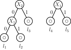
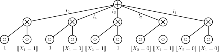
Figure 4: Encoding an additive ensemble of two trees over $\mathbf{X}=\{X_{1},X_{2}\}$ (above) in an omni-compatible circuit over $\mathbf{X}$ (below).

Example D.1 (Decision trees as circuits).

Let $\mathcal{F}$ be an additive ensemble of (decision or regression) trees over variables $\mathbf{X}$, also called a forest, and computing

$$\mathcal{F}(\boldsymbol{x})=\sum_{\mathcal{T}_{i}\in\mathcal{F}}\theta_{i}\mathcal{T}_{i}(\boldsymbol{x})$$

for some input configuration $\boldsymbol{x}\in\mathsf{val}(\mathbf{X})$ and each $\mathcal{T}_{i}$ realizing a tree, i.e., a function of the form

$$\mathcal{T}(\boldsymbol{x})=\sum_{p_{j}\in\mathsf{paths}(\mathcal{T})}l_{j}\cdot\prod_{X_{k}\in{\phi}(p_{j})}\llbracket{x_{k}\leq\delta_{k}}\rrbracket$$

where the outer sum ranges over all possible paths in tree $\mathcal{T}$, $l_{j}\in\mathbb{R}$ is the label (class or predicted real) associated to the leaf of that path, and the product is over indicator functions encoding the decision to take one branch of the tree in path $p_{j}$ if $x_{k}$, the observed value for variable $X_{k}$ appearing in the decision node, i.e., satisfies the condition $\llbracket{x_{k}\leq\delta_{k}}\rrbracket$ for a certain threshold $\delta_{k}\in\mathbb{R}$.

Then, it is easy to transform $\mathcal{F}$ into an omni-compatible circuit $p(\mathbf{X})$ of the form

$${p}(\boldsymbol{x})=\sum_{\mathcal{T}_{i}\in\mathcal{F},p_{j}\in\mathsf{paths}(\mathcal{T_{i}})}l_{j}\cdot\prod_{X_{k}\in{\phi}(p_{j})}\llbracket{x_{k}\leq\delta_{k}}\rrbracket\cdot\prod_{X_{k}^{\prime}\not\in{\phi}(p_{j})}1$$

with a single sum unit realizing the outer sum and as many input product units as paths in the forest, each of which realizing a fully-factorized model over $\mathbf{X}$, and weighted by $l_{j}$. One example is shown in Fig. 4.

Proposition D.3 (Tractable expected predictions of additive ensembles of trees).

Let ${p}$ be a smooth and decomposable PC and $f$ an additive ensemble of $k$ decision trees over variables $\mathbf{X}$ and bounded depth. Then, its expected predictions can be exactly computed in $\mathcal{O}(k\left\lvert{p}\right\rvert)$.

Proof.

Recall that an additive ensemble of decision trees can be encoded as an omni-compatible circuit. Then, proof follows from Cor. B.2.1. ∎

Algorithm 9 RGCtoCircuit($r,\mathsf{cache}_{r},\mathsf{cache}_{s}$)

1:  Input: a regression circuit $r$ over variables $\mathbf{X}$ and two caches for memoization (i.e., $\mathsf{cache}_{r}$ and $\mathsf{cache}_{s}$).

2:  Output: its representation as a circuit $p(\mathbf{X})$.

3:  if $r\in\mathsf{cache}_{r}$ then

4:     return $\mathsf{cache}_{r}(r)$

5:  if $r$ is an input gate then

6:     $p\leftarrow\textsc{Input}(0,{\phi}(r))$

7:  else if $r$ is a sum gate then

8:     ${n}\leftarrow\{\}$

9:     for $i=1$ to $|\mathsf{in}(r)|$ do

10:        ${n}\leftarrow{n}\cup\{\textsc{Support}(r_{i},\mathsf{cache}_{s})\}$

11:        ${n}\leftarrow{n}\cup\{\text{{RGCtoCircuit}}(r_{i},\mathsf{cache}_{r})\}$

12:     ${p}\leftarrow\textsc{Sum}({n},\{\theta_{i},1_{1},\ldots,1_{\mathsf{in}({p})}\}_{i=1}^{|\mathsf{in}(r)|})$

13:  else if $r$ is a product gate then

14:     for $i=1$ to $|\mathsf{in}(r)|$ do

15:        ${p}\leftarrow\textsc{Product}(\{\text{{RGCtoCircuit}}(r_{i},\mathsf{cache}_{r})\}\cup\{\textsc{Support}(r_{j},\mathsf{cache}_{s})\}_{j\neq i})$

16:  $\mathsf{cache}_{r}(r)\leftarrow{p}$

17:  return ${p}$

Proposition D.4 (Tractable expected predictions of deep regressors (regression circuits)).

Let ${p}$ be a structured-decomposable PC over variables $\mathbf{X}$ and $f$ be a regression circuit (Khosravi et al., 2019a) compatible with ${p}$ over $\mathbf{X}$, and defined as

$$f_{n}(\boldsymbol{x})=\begin{cases}0&\text{if $n$ is an input }\\ f_{n_{\mathsf{L}}}(\boldsymbol{x}_{\mathsf{L}})+f_{n_{\mathsf{R}}}(\boldsymbol{x}_{\mathsf{R}})&\text{if $n$ is an AND }\\ \sum_{c\in\mathsf{in}(n)}s_{c}(\boldsymbol{x})\left(\phi_{c}+f_{c}(\boldsymbol{x})\right)&\text{if $n$ is an OR}\end{cases}$$

where $s_{c}(\boldsymbol{x})=\llbracket{\boldsymbol{x}\in\mathsf{supp}(c)}\rrbracket$. Then, its expected predictions can be exactly computed in $\mathcal{O}(\left\lvert p\right\rvert\left\lvert h\right\rvert)$ time and space, where $h$ is its circuit representation as computed by Alg. 9.

Proof.

Proof follows from noting that Alg. 9 outputs a polysize circuit representation $h$ in polytime. Then, computing $\mathbb{E}_{\boldsymbol{x}\sim{p}(\mathbf{X})}\left[h(\boldsymbol{x})\right]$ can be done in $\mathcal{O}(\left\lvert p\right\rvert\left\lvert h\right\rvert)$ time and space by Thm. B.2. ∎

References

- Bach & Jordan (2001) Bach, F. R. and Jordan, M. I. Thin junction trees. In NIPS, volume 14, pp. 569–576, 2001.
- Barrett & Tinelli (2018) Barrett, C. and Tinelli, C. Satisfiability modulo theories. In Handbook of Model Checking, pp. 305–343. Springer, 2018.
- Choi et al. (2013) Choi, A., Kisa, D., and Darwiche, A. Compiling probabilistic graphical models using sentential decision diagrams. In European Conference on Symbolic and Quantitative Approaches to Reasoning and Uncertainty, pp. 121–132. Springer, 2013.
- Choi et al. (2015) Choi, A., Van den Broeck, G., and Darwiche, A. Tractable learning for structured probability spaces: A case study in learning preference distributions. In Proceedings of 24th International Joint Conference on Artificial Intelligence (IJCAI), volume 2015, pp. 2861–2868, 2015.
- Choi et al. (2017) Choi, Y., Darwiche, A., and den Broeck, G. V. Optimal feature selection for decision robustness in bayesian networks. In IJCAI, pp. 1554–1560, 2017.
- Choi et al. (2020) Choi, Y., Vergari, A., and Van den Broeck, G. Probabilistic circuits: A unifying framework for tractable probabilistic modeling. 2020.
- Chow & Liu (1968) Chow, C. and Liu, C. Approximating discrete probability distributions with dependence trees. IEEE transactions on Information Theory, 14(3):462–467, 1968.
- Correia et al. (2020) Correia, A. H. C., Peharz, R., and de Campos, C. P. Joints in random forests. In NeurIPS, 2020.
- Dang et al. (2020) Dang, M., Vergari, A., and Van den Broeck, G. Strudel: Learning structured-decomposable probabilistic circuits. In PGM, Proceedings of Machine Learning Research, 2020.
- Dang et al. (2021) Dang, M., Khosravi, P., Liang, Y., Vergari, A., and Van den Broeck, G. Juice: A julia package for logic and probabilistic circuits. In Proceedings of the 35th AAAI Conference on Artificial Intelligence (Demo Track), Feb 2021.
- Darwiche (2009) Darwiche, A. Modeling and reasoning with Bayesian networks. Cambridge university press, 2009.
- Darwiche (2011) Darwiche, A. Sdd: A new canonical representation of propositional knowledge bases. In Twenty-Second International Joint Conference on Artificial Intelligence, 2011.
- Darwiche & Marquis (2002) Darwiche, A. and Marquis, P. A knowledge compilation map. Journal of Artificial Intelligence Research, 17:229–264, 2002.
- Gibbs & Su (2002) Gibbs, A. L. and Su, F. E. On choosing and bounding probability metrics. International statistical review, 70(3):419–435, 2002.
- Jaeger (2004) Jaeger, M. Probabilistic decision graphs—combining verification and ai techniques for probabilistic inference. International Journal of Uncertainty, Fuzziness and Knowledge-Based Systems, 12(supp01):19–42, 2004.
- Jaeger et al. (2006) Jaeger, M., Nielsen, J. D., and Silander, T. Learning probabilistic decision graphs. International Journal of Approximate Reasoning, 42(1-2):84–100, 2006.
- Jenssen et al. (2006) Jenssen, R., Principe, J. C., Erdogmus, D., and Eltoft, T. The cauchy–schwarz divergence and parzen windowing: Connections to graph theory and mercer kernels. Journalof the Franklin Institute, 343(6):614–629, 2006.
- Jerrum & Sinclair (1993) Jerrum, M. and Sinclair, A. Polynomial-time approximation algorithms for the ising model. SIAM Journal on computing, 22(5):1087–1116, 1993.
- Jurkat (1965) Jurkat, W. B. On cauchy’s functional equation. Proceedings of the American Mathematical Society, 16(4):683–686, 1965.
- Kampa et al. (2011) Kampa, K., Hasanbelliu, E., and Principe, J. C. Closed-form cauchy-schwarz pdf divergence for mixture of gaussians. In The 2011 International Joint Conference on Neural Networks, pp. 2578–2585. IEEE, 2011.
- Khosravi et al. (2019a) Khosravi, P., Choi, Y., Liang, Y., Vergari, A., and Van den Broeck, G. On tractable computation of expected predictions. In Advances in Neural Information Processing Systems, pp. 11169–11180, 2019a.
- Khosravi et al. (2019b) Khosravi, P., Liang, Y., Choi, Y., and den Broeck, G. V. What to expect of classifiers? reasoning about logistic regression with missing features. In IJCAI, pp. 2716–2724, 2019b.
- Khosravi et al. (2020) Khosravi, P., Vergari, A., Choi, Y., Liang, Y., and den Broeck, G. V. Handling missing data in decision trees: A probabilistic approach. In Proceedings of The Art of Learning with Missing Values, Workshop at ICML, 2020.
- Kisa et al. (2014) Kisa, D., Van den Broeck, G., Choi, A., and Darwiche, A. Probabilistic sentential decision diagrams. In Proceedings of the 14th international conference on principles of knowledge representation and reasoning (KR), pp. 1–10, 2014.
- Koller & Friedman (2009) Koller, D. and Friedman, N. Probabilistic graphical models: principles and techniques. MIT press, 2009.
- Liang & Van den Broeck (2017) Liang, Y. and Van den Broeck, G. Towards compact interpretable models: Shrinking of learned probabilistic sentential decision diagrams. In IJCAI 2017 Workshop on Explainable Artificial Intelligence (XAI), August 2017.
- McLachlan et al. (2019) McLachlan, G. J., Lee, S. X., and Rathnayake, S. I. Finite mixture models. Annual review of statistics and its application, 6:355–378, 2019.
- Minka (2001) Minka, T. P. Expectation propagation for approximate bayesian inference. In UAI, pp. 362–369. Morgan Kaufmann, 2001.
- Molina et al. (2019) Molina, A., Vergari, A., Stelzner, K., Peharz, R., Subramani, P., Di Mauro, N., Poupart, P., and Kersting, K. Spflow: An easy and extensible library for deep probabilistic learning using sum-product networks. arXiv preprint arXiv:1901.03704, 2019.
- Moral et al. (2001) Moral, S., Rumí, R., and Salmerón, A. Mixtures of truncated exponentials in hybrid bayesian networks. In ECSQARU, volume 2143 of Lecture Notes in Computer Science, pp. 156–167. Springer, 2001.
- Nielsen (2012) Nielsen, F. Closed-form information-theoretic divergences for statistical mixtures. In Proceedings of the 21st International Conference on Pattern Recognition (ICPR2012), pp. 1723–1726. IEEE, 2012.
- Opper et al. (2005) Opper, M., Winther, O., and Jordan, M. J. Expectation consistent approximate inference. Journal of Machine Learning Research, 6(12), 2005.
- Oztok et al. (2016) Oztok, U., Choi, A., and Darwiche, A. Solving -complete problems using knowledge compilation. In Proceedings of the 15th International Conference on Principles of Knowledge Representation and Reasoning (KR), pp. 94–103, 2016.
- Peharz et al. (2019) Peharz, R., Vergari, A., Stelzner, K., Molina, A., Trapp, M., Shao, X., Kersting, K., and Ghahramani, Z. Random sum-product networks: A simple and effective approach to probabilistic deep learning. In UAI, volume 115 of Proceedings of Machine Learning Research, pp. 334–344. AUAI Press, 2019.
- Peharz et al. (2020) Peharz, R., Lang, S., Vergari, A., Stelzner, K., Molina, A., Trapp, M., Broeck, G. V. d., Kersting, K., and Ghahramani, Z. Einsum networks: Fast and scalable learning of tractable probabilistic circuits. In International Conference of Machine Learning, 2020.
- Pipatsrisawat & Darwiche (2008) Pipatsrisawat, K. and Darwiche, A. New compilation languages based on structured decomposability. In AAAI, volume 8, pp. 517–522, 2008.
- Poon & Domingos (2011) Poon, H. and Domingos, P. Sum-product networks: A new deep architecture. In 2011 IEEE International Conference on Computer Vision Workshops (ICCV Workshops), pp. 689–690. IEEE, 2011.
- Rabiner & Juang (1986) Rabiner, L. and Juang, B. An introduction to hidden markov models. ieee assp magazine, 3(1):4–16, 1986.
- Rahman et al. (2014) Rahman, T., Kothalkar, P., and Gogate, V. Cutset networks: A simple, tractable, and scalable approach for improving the accuracy of chow-liu trees. In Joint European conference on machine learning and knowledge discovery in databases, pp. 630–645. Springer, 2014.
- Rényi et al. (1961) Rényi, A. et al. On measures of entropy and information. In Proceedings of the Fourth Berkeley Symposium on Mathematical Statistics and Probability, Volume 1: Contributions to the Theory of Statistics. The Regents of the University of California, 1961.
- Rooshenas & Lowd (2014) Rooshenas, A. and Lowd, D. Learning sum-product networks with direct and indirect variable interactions. In International Conference on Machine Learning, pp. 710–718. PMLR, 2014.
- Sahoo & Kannappan (2011) Sahoo, P. K. and Kannappan, P. Introduction to functional equations. CRC Press, 2011.
- Shen et al. (2016) Shen, Y., Choi, A., and Darwiche, A. Tractable operations for arithmetic circuits of probabilistic models. In Advances in Neural Information Processing Systems, pp. 3936–3944, 2016.
- Shih & Ermon (2020) Shih, A. and Ermon, S. Probabilistic circuits for variational inference in discrete graphical models. In NeurIPS, 2020.
- Shih et al. (2019) Shih, A., den Broeck, G. V., Beame, P., and Amarilli, A. Smoothing structured decomposable circuits. In NeurIPS, pp. 11412–11422, 2019.
- Tran et al. (2021) Tran, L., Pantic, M., and Deisenroth, M. P. Cauchy-schwarz regularized autoencoder. arXiv preprint arXiv:2101.02149, 2021.
- Vergari et al. (2015) Vergari, A., Di Mauro, N., and Esposito, F. Simplifying, regularizing and strengthening sum-product network structure learning. In Joint European Conference on Machine Learning and Knowledge Discovery in Databases, pp. 343–358. Springer, 2015.
- Wei & Gibson (2001) Wei, B. and Gibson, J. D. Comparison of distance measures in discrete spectral modeling. Master’s thesis, Citeseer, 2001.
- Xu et al. (2018) Xu, J., Zhang, Z., Friedman, T., Liang, Y., and den Broeck, G. V. A semantic loss function for deep learning with symbolic knowledge. In ICML, volume 80 of Proceedings of Machine Learning Research, pp. 5498–5507. PMLR, 2018.
- Zeng et al. (2020) Zeng, Z., Morettin, P., Yan, F., Vergari, A., and den Broeck, G. V. Scaling up hybrid probabilistic inference with logical and arithmetic constraints via message passing. In ICML, volume 119 of Proceedings of Machine Learning Research, pp. 10990–11000. PMLR, 2020.