The Stars of the HETDEX Survey. I. Radial Velocities and Metal-Poor Stars from Low-Resolution Stellar Spectra

Abstract

The Hobby-Eberly Telescope Dark Energy Experiment (HETDEX) is an unbiased, massively multiplexed spectroscopic survey, designed to measure the expansion history of the universe through low-resolution ($R\sim 750$) spectra of Lyman-Alpha Emitters. In its search for these galaxies, HETDEX will also observe a few 10⁵ stars. In this paper, we present the first stellar value-added catalog within the internal second data release of the HETDEX Survey (HDR2). The new catalog contains 120,571 low-resolution spectra for 98,736 unique stars between $10<G<22$ spread across the HETDEX footprint at relatively high ($b\sim 60^{\circ}$) Galactic latitudes. With these spectra, we measure radial velocities (RVs) for $\sim$42,000 unique FGK-type stars in the catalog and show that the HETDEX spectra are sufficient to constrain these RVs with a 1$\sigma$ precision of 28.0 km s^-1 and bias of 3.5 km s^-1 with respect to the LAMOST surveys and 1$\sigma$ precision of 27.5 km s^-1 and bias of 14.0 km s^-1 compared to the SEGUE survey. Since these RVs are for faint ($G\geq 16$) stars, they will be complementary to Gaia. Using t-Distributed Stochastic Neighbor Embedding (t-SNE), we also demonstrate that the HETDEX spectra can be used to determine a star’s $T_{\mathrm{eff}}$, and log $g$ and its [Fe/H]. With the t-SNE projection of the FGK-type stars with HETDEX spectra we also identify 416 new candidate metal-poor ([Fe/H] $<-1$ dex) stars for future study. These encouraging results illustrate the utility of future low-resolution stellar spectroscopic surveys.

1 Introduction

One of the primary goals within Galactic astronomy is to constrain the nature of the physical processes that govern how the Milky Way formed, assembled, and evolved from its birth to today. The key observational data that constrains theories of Milky Way formation include the position, velocities, and stellar atmospheric parameters for millions of stars across the Galaxy. This is what has given rise to missions such as Gaia, which have enabled the detailed study of the positions and velocities for $\sim$1.7 billion stars through precise astrometric data (Gaia Collaboration et al., 2018), and has also been a key driver for the creation of large multi-object stellar spectroscopic surveys. Stellar spectra, whether at low- or high-resolution, are particularly useful because they enable not only measurement of the radial velocity (RV) of stars, giving us 3-D velocity information when combined with Gaia, but also they contain critical information, including the effective temperature ($T_{\mathrm{eff}}$), surface gravity (log $g$), metallicity ([Fe/H]), and chemical abundance ratios ([X/Fe]), for large samples of stars.

Large spectroscopic surveys have been instrumental in uncovering the history and nature of our Milky Way Galaxy and beyond. These projects have obtained data, which range from low-to-high resolution. For example, while the primary goal of the original the Sloan Digital Sky Survey (SDSS, York et al., 2000) was to map galaxies and quasars across the universe, the survey also obtained low-resolution (R$\sim$2000) spectra for $\sim 10^{5}$ stars through the Sloan Extension for Galactic Understanding and Exploration (SEGUE, Yanny et al., 2009). Similar to SEGUE, the most recent data release (DR5) from the Large Sky Area Multi-Object Fibre Spectroscopic Telescope survey (LAMOST DR5, Luo et al., 2015; Xiang et al., 2017) contains low-resolution (R$\sim$1800) spectra for over 8 million stars. At moderate resolution (R$\sim$7500), the magnitude-limited Radial VElocity Experiment (RAVE, Steinmetz et al., 2006, 2020), whose aim was to explore the structure and nature of the Milky Way, observed more than half a million stars observed in the southern hemisphere and derive not only RV informaiton but also stellar atmospheric parameters for their sample.

Moving towards higher resolution the GALactic Archaeology with HERMES (GALAH, De Silva et al., 2015; Buder et al., 2018) survey has obtained optical spectra of 342,682 stars at R$\sim$28,000, the SDSS-IV Apache Point Observatory Galactic Evolution Experiment (APOGEE, Majewski et al., 2017; Ahumada et al., 2019, Jönsson et al. in prep.) survey has collected infrared (H-band) spectra for upwards of 400,000 stars at R$\sim$21,000, and the Gaia-ESO survey (Gilmore et al., 2012) aims to collect up to 100,000 spectra at R$\sim$47,000. As one moves toward higher resolution, sample sizes decrease because of the tradeoff that exists between the resolution of the spectrograph and the exposure time required to obtain high signal-to-noise ratio (SNR) data required for the scientific aims of the surveys.

With high resolution, it is possible to derive both the detailed stellar atmospheric parameters ($T_{\mathrm{eff}}$, log $g$, [Fe/H]) and the chemical abundance ratios, denoted as [X/Fe], for many elements. This is the case for surveys like APOGEE, GALAH, and Gaia-ESO. However, for lower resolution spectroscopic surveys (e.g., SDSS, LAMOST), it becomes significantly more challenging to recover the stellar parameters and detailed chemical fingerprint. In fact, until recently, many low-resolution surveys only were able to determine the $T_{\mathrm{eff}}$, log $g$, [Fe/H], and, in some cases, [$\alpha$/Fe] (e.g., Lee et al., 2008a, 2015; Boeche et al., 2018). Despite this limitation, Ting et al. (2017) demonstrated that it may be possible to measure not only the stellar atmospheric parameters but also several key individual elements down to R$\gtrapprox$700 with precisions at the $\sim$0.15 dex level. While, at first, the results from these authors seem surprising, Xiang et al. (2019) illustrated the power of new machine learning techniques and derived the stellar parameters and 16 [X/Fe] atmospheric abundance ratios from the low-resolution (R$\sim$1800) LAMOST spectra. Additionally, other works have shown that it is possible to uncover metal-poor stars from low-resolution (R$<$ 1000) spectra (e.g. Aguado et al., 2019) and even from photometry (e.g. Starkenburg et al., 2017; Casagrande et al., 2019; Lucey et al., 2019).

These new low-resolution techniques offer many opportunities including discovering and characterizing relatively rare, yet scientifically important, metal-poor stars. Metal-poor stars, defined as those with [Fe/H] $<$ $-1.0$ dex, are important because they offer insights into the early Galaxy as well as constrain the nucleosynthesis of the elements (e.g. Bromm & Larson, 2004; Beers & Christlieb, 2005; Karlsson et al., 2013; Yong et al., 2013; Roederer et al., 2014; Frebel & Norris, 2015; Sakari et al., 2018, and references therein). These stars are pretty rare yet their chemical properties are highly sought after. Hunting metal-poor star, especially those at the lowest metallicities is still an critical task. Several low- to medium-resolution surveys have been instrumental in finding and characterizing these metal-poor stars (e.g. Aoki et al., 2008; Ruchti et al., 2010; Xu et al., 2013; Matijevič et al., 2017; Li et al., 2018).

In this context, the Hobby-Eberly Telescope Dark Energy Experiment (HETDEX, Hill et al., 2008; Hill & HETDEX Consortium, 2016, Gebhardt et al., in prep.) is a low-resolution (R$\sim$750) blind spectroscopic survey whose primarily goal is to map the locations and redshifts of high-$z$ Lyman-$\alpha$ emitting galaxies to constrain the nature of dark energy. This survey will cover a total of $\sim$450 sq. deg. However, much like the case for SDSS, which was designed for cosmological investigations but eventually observed many stars, HETDEX will obtain spectra for large numbers of stars in its search for Lyman-$\alpha$ emitters. The unbiased nature of HETDEX (i.e., no pre-selection of objects is done), makes it extremely powerful, when compared to other large stellar spectroscopic surveys, to answer questions about the properties of the Milky Way. Therefore, we explore the use of these low-resolution HETDEX data for stellar astrophysics applications, such as deriving radial velocities for faint stars in the Gaia catalogue and finding rare, but scientifically critical, metal-poor stars using machine learning. This is the first time these techniques have been applied to this dataset.

This paper is structured as follows: Section 2 details the spectroscopic data collected from the HETDEX survey and presents the HETDEX-Gaia value added catalogue. We also describe the overlap data set used to validate our methods. In section 3 we describe the methods used to constrain the RVs for the FGK-type stars found in the HETDEX survey and the t-distributed Stochastic Neighbor Embedding (tSNE) machine learning method that we used to uncover candidate metal-poor stars. Section 4 presents the results of the RV and tSNE analysis and discusses the role HETDEX may play in constraining the nature of the Galaxy. Finally, in section 5 we summarize our results and describes several future possible investigations with the data presented here.

2 Data

2.1 The HETDEX Survey

The HETDEX survey, which aims to constrain the nature of dark energy by observing Lyman-$\alpha$ emitters in the redshift interval 1.9 $\leq z\leq$ 3.5, is currently being carried out on the Hobby-Eberly Telescope (HET; Ramsey et al. 1994), which is an 11-m telescope with a segmented primary mirror, recently upgraded with a 22 arcmin field of view and 10 m pupil (Hill et al., 2018a). The upgraded HET includes a key new instrument called the Visible Integral-field Replicable Unit Spectrograph (VIRUS, Hill, 2014; Hill et al., 2018b), which is a massively replicated, fiber-fed integral field spectrograph designed specifically to preform unbiased spectroscopic surveys. The entire VIRUS instrument consists of up to 156 integral field low-resolution (resolving power, $R\sim$750) spectrographs, arrayed in 78 pairs. Each of the 78 VIRUS units is fed by 448 $1\farcs 5$ fibers. Each of the fibers are fed to individual spectrographs (two per IFU) and dispersed onto CCD detectors at a mostly equal spacing on the detector. The spectrographs have a fixed spectral window in the optical with 3500 $<\lambda<$ 5500 Å with 2 Å pixels. This represents a pixel size of $\sim$130 km s^-1. At full deployment, VIRUS will be able to capture 34,944 spectra for each exposure. The instrumentation for HETDEX is described in Hill et al., 2021, in preparation. The HETDEX survey, which is currently underway with the VIRUS instrument, will be an blind emission line survey of an area on the sky comprising of $\sim 450$ sq. deg with a 1/4.5 fill factor. The current release of HETDEX contains data from $\sim$29.85 sq. deg, or $\sim$30% of the expected final HETDEX dataset. Figure 1, shows the location of the main HETDEX survey footprint (black) and a density map of 2 million randomly selected stars from the Gaia mission. The background collection of stars from Gaia is to provide a Galactic context to the HETDEX fields. Also shown is the Galactic coordinates of the stars (section 2.2) in this data release of the HETDEX survey (red points).

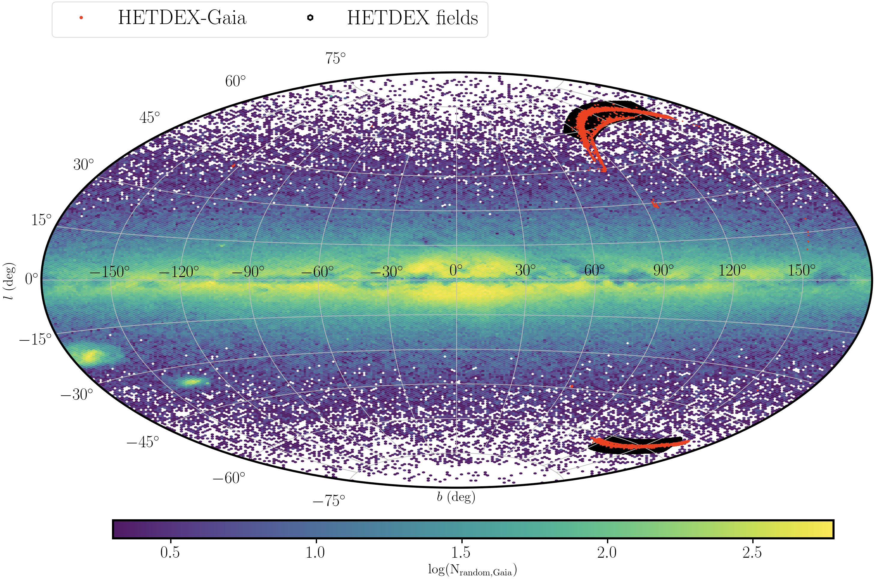
Figure 1: An Aitoff projection of the Galactic coordinates for the HETDEX fields (black pentagons) and stars observed in this data release (red circles). For reference, we also show positions for 2 million randomly selected stars from the Gaia mission. While most of the stars lie in the main HETDEX footprint (at high Galactic latitude), there are some that can also be found in early calibration and extension fields.

Each HETDEX pointing consists of a set of 3-dithered 6 min exposures (done in order to fill the sky gaps between fibers; Gebhardt et al., 2021 in preparation). The HETDEX fields are mostly at high Galactic latitude, with a median absolute Galactic latitude of $\sim$60 deg (see Figure 1). In HETDEX’s quest to survey $\sim 10^{6}$ Lyman-$\alpha$ emitters, it will also capture spectra for many ($\sim 10^{5}$) stars. It is these stars that are the subject of this work. We make use of the second internal data release for the HETDEX survey, which we will refer to as iHDR2.

2.2 The HETDEX-Gaia Value Added Catalog

The primary goal of this work is to build a catalouge of stellar spectra from observed within the HETDEX survey and use those spectra to (1) measure RVs for Gaia sources and (2) find metal-poor candidate stars. To achieve these aims we must first obtain a list of point sources (i.e., stars) in the HETDEX survey. This task is accomplished by cross matching each centroid of each fiber pointing that exists in iHDR2, which includes $\sim$200 million spectra, against the $\sim$1.7 billion point sources in the Gaia DR2 catalogue (Gaia Collaboration et al., 2018). In order to determine the stars in common between HETDEX and Gaia, we cross-match each fiber center in iHDR2 with Gaia DR2 using a generous 3″ search radius in RA and DEC. This relatively large cross-match radius compared to the $1\farcs 5$ fiber diameter of VIRUS ensures that we capture the stars that overlap between HETDEX and Gaia DR2. The result of this cross match is referred to as the HETDEX-Gaia value added catalogue. We note that distant galaxies can also appear as point sources and therefore we expect some level of contamination from galaxies in our sample.

Table 1: The HETDEX-Gaia Value Added Catalogue

Gaia Source ID	RA	DEC	$G$	$BP-RP$	SNRHETDEX	RV	$\sigma$RV	Barycentric Correction	…
	(deg)	(deg)	(mag)	(mag)	(pixel-1)	(km s-1)	(km s-1)	(km s-1)
2543173457359409664	9.78194	–0.00009	13.06	0.92	58.73	–8.49	28.62	4.18	….
2543068690220755456	10.45149	0.00748	19.15	1.90	3.58	–192.69	62.57	4.19	….
2543068690220758144	10.45224	0.01046	18.88	1.90	5.73	75.98	45.75	4.19	….
2543092398440275072	10.49391	0.05285	20.32	0.81	5.73	–206.13	63.73	4.22	….
2543733211856949120	6.67326	–0.02982	17.51	1.12	29.14	–17.25	19.08	–6.87	….
2543740010789142528	6.84129	0.01837	20.58	1.08	4.21	–55.21	22.88	–6.78	….
2543735509663099648	6.84963	–0.00984	19.52	1.55	7.90	–14.42	35.71	–6.78	….
2543040137278030848	10.73567	–0.04865	17.18	1.85	20.31	–11.99	57.23	–4.99	….
2543039381363775232	10.74644	–0.05880	20.23	1.58	2.64	51.64	50.80	–4.99	….
2543041030631244928	10.79130	–0.03320	19.38	1.74	4.69	–90.57	40.68	–4.96	….
2543041408588483968	10.86433	0.00056	19.81	1.27	5.91	–272.85	137.26	5.40	….
2543175415864489472	9.61114	–0.01187	17.25	1.29	48.19	–471.99	143.30	4.10	….
2543172009953849344	9.62519	–0.04361	19.58	1.08	10.82	–111.52	18.64	4.10	….
2543174728669728768	9.75072	0.05631	19.33	1.33	27.20	2.98	32.01	4.18	….
2543174385072345216	9.77910	0.02872	17.40	1.27	30.14	–56.76	25.57	4.19	….
2543173457359409664	9.78194	–0.00009	13.06	0.92	95.78	28.80	14.25	4.18	….
2543736579111320448	6.96626	0.01918	17.92	1.34	20.29	–17.54	20.59	–7.54	….
2543831343269590656	7.00635	0.06922	12.79	0.89	65.11	–24.53	12.01	–7.51	….
2543547463111076864	7.06080	–0.05459	14.78	0.90	68.92	–70.10	11.09	–7.51	….
2543642295989347840	7.08448	–0.00604	16.59	1.42	35.53	25.00	24.06	–7.49	….
…	…	…	…	…	…	…	…	…	…

NOTE: This is a subsample of the full HETDEX-Gaia value added catalogue. The Gaia DR2 source identifier of each star is given in column 1 with equatorial coordinates (in J2015.5) in columns 2 and 3. The Gaia $G$ band magnitude and the $BP-RP$ color for each star are listed in columns 4 and 5, respectively. The average signal to noise ratio (SNR) per pixel estimated using the HETDEX spectra is given in column 6. The RV and its uncertainty measured from cross-correlating the HETDEX spectra against a template spectrum are listed in columns 7 and 8, respectively. The heliocentric correction, used to correct the measured RV into the rest frame of the Sun, can be found in column 9. This is only a subsample of the full table, which will be provided online, illustrate the the catalogue’s format.

Figure 2: The median SNR per pixel for each star of the 98,736 stars in the HETDEX-Gaia catalogue as a function of their Gaia $G$ band magnitude. The black dashed line represents the SNR = 5 pixel^-1; we generally focus on the $\sim$47,000 sources above this line.

The final HETDEX-Gaia value added catalogue contains 98,736 unique point sources in the Gaia DR2 catalogue with spectral data from HETDEX. Table 1 is subsample of the observational and spectroscopic properties of this catalogue. The full catalogue will be available online. With the cross-match in hand, we re-extracted the HETDEX spectra at the Gaia DR2 positions accounting for proper motion on the date of the HETDEX observation. If a Gaia DR2 source was observed on multiple nights, multiple independent extractions we preformed. We used an optimal method (Horne, 1986) for extraction that employs a Moffat spatial profile (Moffat, 1969) set to the seeing conditions of the observation as well as a maximum aperture of 3″.

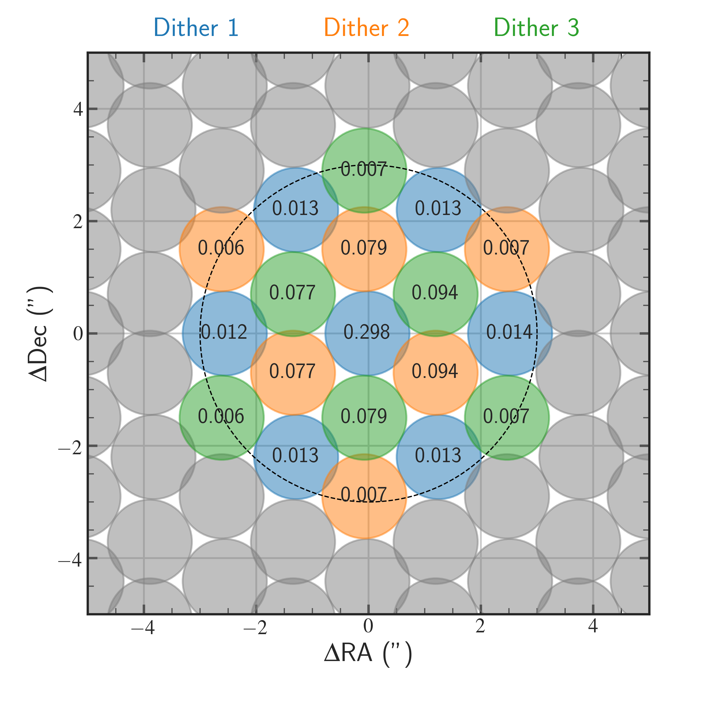
Figure 3: The fiber layout for an example source in an observation with 1.8” seeing. The source being at $\Delta$RA = $\Delta$DEC = 0. A HETDEX observation includes three dithers shown in blue, orange, and green. The fiber diameter is 1.5” and in this example since the closest fiber from dither 1 is nearly centered on the source for extraction, it contains roughly 30% of the total light from the Moffat spatial profile. We show the 3” extraction aperture as a dashed black line and the aperture includes all fibers that overlap that radius. We show the fiber coverage for each of the extracted fibers and these coverage values serve as the weights in our optimal extraction. In total 94% of the light is captured in the highlighted fibers. The fibers outside of the extraction aperture are all grey.

To perform extractions for any individual source we collect all fibers within 7 arcseconds. We use the seeing conditions of the observation to construct a Moffat spatial profile (Moffat 1969) and we integrate that profile over the 1.5 arcsecond diameter fibers. The integral of the profile over the fiber is called the covering fraction. This covering fraction depends on the distance of the source from the fiber center, the seeing conditions, and the wavelength as the HET does not correct for differential atmospheric refraction so the position of a source with respect to the fiber location changes as a function of wavelength. We illustrate the fiber coverage fractions in Figure 3. We use these fractions as weights in an optimal extraction (Horne, 1986). Each extracted spectrum includes the calibrated flux (in units of $\times 10^{-17}$ ergs cm^-2 s^-1), a 1$\sigma$ error array, and a fiber coverage array. The fiber coverage array is defined as the fraction of light that the HETDEX fibers collect for a given point source at a given wavelength. The sky background is estimated using the biweight of all fibers in the observation after the fibers have been flat-fielded using twilight observations. We do not remove contamination from nearby sources. We exclude sources for which fiber coverage arrays contained only pixels with coverages less than 5% (i.e., where $<$5% of its light from the star made it into all extracted fibers). Detailed information on the re-extraction methods is included in Zeimann et al. (2021, in preparation).

In addition, we also computed a ‘continuum normalized’ version of the spectral fluxes, which are normalized using the boosted median continuum (henceforth BMC, e.g., Rogers et al., 2010; Hawkins et al., 2014). In this approach, the continuum to be divided is defined as a prescribed percentile of the flux in a predefined window. This is a common approach for low-resolution spectra for which the true continuum is extremely difficult to define due to significant line blending. For the purposes of the HETDEX spectra, we choose a window size of 50 Å (i.e., 25 pixels) and a percentile of 98%. Additionally, we masked any pixel in the spectra that had low ($<$ 50%) fiber coverage (i.e., where less than 50% of the light at a given wavelength from the source falls within the extracted fibers. We filled these masked pixels by interpolating the higher coverage pixels around the masked value(s).

We determined the signal-to-noise ratio (SNR) for each spectrum by dividing the flux by the flux uncertainty for each pixel and taking the median over the full spectral range. Figure 2 shows the computed median SNR per pixel for the stars in the HETDEX-Gaia value added catalogue as a function of their $G$ band magnitude. We generally focus on the 46,890 unique sources with SNR $>$ 5 pixel^-1 in this work. As expected, for a constant exposure time, stars brighter in Gaia $G$ band have significantly higher SNR. We note that there are likely issues with the brightest stars as they are affected by significant and complex scattered light. HETDEX saturates around $G\sim$ 14 mag, and for sources brighter than $G\sim$ 15 mag the masking procedures can be aggressive and mistake bright spectra for cosmic rays. The observed distribution in parallax ($\varpi$), $G$, and $BP-RP$ color for stars with SNR $>$ 5 pixel^-1 can be found in Figure 4. These distributions demonstrate that the most HETDEX stars are farther than 1 kpc, fainter than G $>$ 18, and have colors near the turn-off.

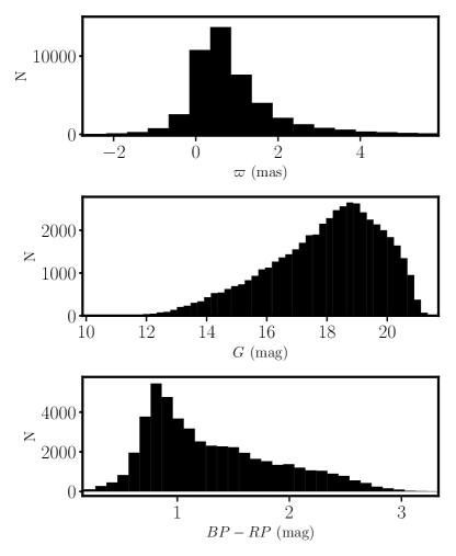
Figure 4: The distribution of parallax ($\varpi$, top panel), $G$ band magnitude (middle panel), and $BP-RP$ color (bottom panel) for the stars whose SNR $>$ 5.

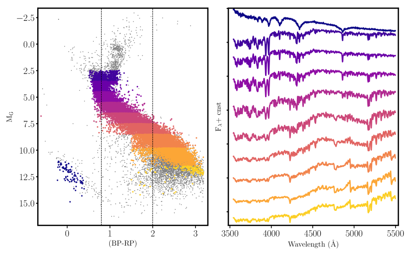
Figure 5: Left panel: The color-magnitude diagram of the Gaia-HETDEX value added catalogue for stars for which the parallax uncertainty is less than 30% (gray points). The dotted black lines represent the color range $0.8<BP-RP<2.0$, which we focus on in this work. Right panel: The median combined spectra for stars in different regions of the color magnitude diagram with SNR $>$ 5. Spectra are offset by a constant in order visualize them on the same plot. Each star represented by a colored circle in the left panel was used to generate the median stacked spectrum (with the same color) in the right panel.

To illustrate the stars uncovered in the HETDEX survey as well as their spectral quality, in the left panel of Figure 5 we show the Gaia color-magnitude diagram for those stars of the HETDEX-Gaia value added catalogue with Gaia parallax uncertainty of less than 30%. The color used for this work is the difference of the Gaia blue ($BP$) and red ($RP$) passbands. For this illustrative plot, we invert the parallaxes to obtain the distance and subsequently the absolute $G$ band magnitude. However, we note that for larger uncertainties one should not invert the parallax but rather infer the distance given the parallax (e.g., Bailer-Jones, 2015; Astraatmadja & Bailer-Jones, 2016). We also do not apply reddening corrections to these colors because HETDEX fields were chosen explicitly to have relatively low (i.e., E($B-V$) $<$ 0.05) extinction. To illustrate the typical HETDEX spectra for different spectral types we median-combine (or stack) stars across 10 absolute magnitude-color bins, which encapsulate the OBAFGKM-type stars (from blue to yellow, respectively) as well as white dwarfs (dark blue), that are represented by the colors on the left panel of the figure. The spectral stacks contain a hundred (white dwarfs) to a few thousand (G-type) of spectra. Stars that are denoted by gray points are those which are not used for the median stack due to low SNR (SNR $<$ 5). The right side of Figure 5 shows the median-stacked spectra for white dwarfs to OBAFGKM-type stars from top to bottom. The vertical axis represents the median flux with an additive constant to offset the spectra for the purposes of visualization. Figure 5 shows that HETDEX spectra are of high enough resolution and quality to identify key stellar features (e.g., Ca H&K, CH G-band, H$\beta$, Mg Triplet, TiO molecular band head, etc.).

2.3 Other Large Spectroscopic Surveys: LAMOST and SDSS

To better understand the information content of the HETDEX spectra relative to other large multi-object spectroscopic surveys, we have matched several of these surveys with the HETDEX-Gaia value added catalogue described in Section 2.1. The cross matches were preformed with the fifth data release of the LAMOST survey, the sixteenth data release of the APOGEE survey, and the ninth data release of the SEGUE survey. These matches were accomplished by using a $1\farcs 5$ search window in each of the surveys centered around each point source in the HETDEX-Gaia catalogue. We did not cross match against southern hemisphere spectroscopic surveys (e.g., Gaia-ESO, GALAH, RAVE) because HETDEX was carried out in the Northern hemisphere and thus we do not expect many overlapping stars.

The cross match with the above three surveys have 6,364 point sources in common with the LAMOST survey (HETDEX-LAMOST catalogue), 5,730 point sources in common with the SEGUE survey (HETDEX-SEGUE catalogue), and 658 point sources in common with the APOGEE survey. In Table 2, we summarize the depth, resolution, and overlap between the surveys discussed above. It is clear from Table 2, that HETDEX will cover a magnitude space that few stellar spectroscopic surveys cover. Given the low sample size in the cross match with the APOGEE survey, we will not consider HETDEX-APOGEE cross matches subsequently in this paper.

Table 2: The Overlap between HETDEX and other large surveys

Survey	$\overline{G}$	$\sigma G$	Overlap N	Resolution
	(mag)	(mag)
HETDEX	18.8	2.1	…	750
SEGUE	17.2	1.3	5730	2000
LAMOST	15.1	1.9	6364	1800
APOGEE	13.5	2.1	658	22500

NOTE: Summary of the overlap between HETDEX and other large spectroscopic surveys. Each survey considered is shown in column 1. The average ($\overline{G}$) and standard deviation ($\sigma G$) of the Gaia $G$ band magnitude that the survey covers can be found in column 2 and 3, respectively. The overlap between HETDEX and each survey and its resolution is displayed in columns 4 and 5, respectively.

For a reliable comparison, we use only a subset of the HETDEX-LAMOST and HETDEX-SEGUE catalogues. For the HETDEX-LAMOST catalogue, we require the following: (1) the absolute value of the LAMOST RV to be less than 600 km s^-1, (2) the uncertainty in RV to be less than 10 km s^-1, (3) the LAMOST SNR in the $G$ band must be larger than 5. The first three constraints were designed to ensure that the LAMOST RV is fairly well determined. Additionally, we require (1) the absolute value of the HETDEX measured RV be less than 600 km s^-1, (2) the uncertainty in the HETDEX RV be less than 50 km s^-1, and (3) the HETDEX SNR be larger than 5. These last three criteria were required to ensure that reasonable RVs were determined from the HETDEX spectra. For example, when the HETDEX measured RV uncertainty is larger than 50 km s^-1, which happens for a small number of stars in the HETDEX-LAMOST and HETDEX-SEGUE datatsets, the RVs are not likely to be reliable. Together these constraints reduced the overall HETDEX-LAMOST catalogue to 2,384 stars for RV comparisons with a median HETDEX SNR = 60 pixel^-1. We also impose the same set of quality criteria on the HETDEX-SEGUE catalogue, which reduced the comparison sample to 1,456 stars, with a median HETDEX SNR = 30 pixel^-1. These comparison samples enable robust quantification of the external precision with which we can estimate RVs using the HETDEX spectra (see Section 4.1).

3 Methods

The primary aims of this paper are to present the first stellar spectra for the HETDEX survey, determine the RVs for the HETDEX-Gaia value added catalogue and find any candidate metal-poor stars hidden within the low-resolution data. As such, in the following sections, we outline the methods used to measure the RVs from HETDEX spectra (Section 3.1) and identify potential metal-poor candidate stars (Section 3.2).

3.1 Radial Velocities

The RVs for HETDEX spectra are determined using the cross-correlation technique, whereby the observed spectrum is compared to a template spectrum. To do this, we made use of the iSpec python package (Blanco-Cuaresma et al., 2014). iSpec cross correlates the observed spectra with a template spectrum within a specific velocity range and step. A grid of RV template spectra were generated using the TURBOSPECTRUM (Alvarez & Plez, 1998; Plez, 2012) radiative transfer package along with the MARCS model atmosphere grid (Gustafsson et al., 2008) and version 5 of the Gaia-ESO  linelist (Heiter et al., submitted). The same spectral synthesis configuration is also used in Hawkins et al. (2020), although here it is at much lower spectral resolution. These template spectra were generated with a wavelength coverage of 3500 $<\lambda<$ 5500 Å with a resolution of R = 750 to approximately match the HETDEX spectra. The grid was generated for temperatures between 4000 $<$ $T_{\mathrm{eff}}$ $<$ 7000 K in steps of 250 K, log gravities from 0.5 $<$ log $g$ $<$ 5.0 dex in steps of 0.5 dex, and metallicities between $-2.0<$ [Fe/H] $<+0.5$ dex in steps of 0.50 dex. Given the temperature range of the grid, we restrict our further analysis to stars with 0.8 $<(BP-RP)<$ 2.0.

Once the RV template grid was constructed, each HETDEX spectrum was matched to one of the template spectra by minimizing the $\chi^{2}$. The template spectral grid was also normalized using the BMC to be consistent with the observed spectra. The cross correlation is done in velocity space with RVs between $-1000<$ RV $<$ +1000 km s^-1 and a velocity step of 1 km s^-1. iSpec determines the RV by fitting a second order polynomial near the peak of the cross correlation function, and indicates if there are multiple peaks in the cross correlation, which could represent the presence of a binary companion. After the RVs are determined for each star, the barycentric correction using iSpec is applied to the RV. As noted in the iSpec documentation, the uncertainties in the RV are determined using the cross correlation function and its second derivative according to Zucker (2003).

3.2 Categorizing the HETDEX Stars using Machine Learning: t-SNE

In addition to measuring the RVs for HETDEX stellar spectra, we are also interested in identifying any metal-poor stars in these low-resolution data, as this has not yet been done for this dataset. One way of categorizing stars on the basis of how similar their spectra appear is through the t-Distributed Stochastic Neighbor Embedding (tSNE, van der Maaten & Hinton, 2008). tSNE is a machine learning technique that enables the construction of a low dimensional (D), normally 2 dimensional (2-D), projection of a higher dimensional dataset while efficiently retaining much its original complexity. tSNE has been used by several other surveys to characterize their stellar spectra. For example, it has been employed by Matijevič et al. (2017) to find very metal-poor stars in the RAVE survey, by Anders et al. (2018) to explore the practicality for chemical tagging purposes with high-resolution data taken with the HARPS spectrograph, and by Jofré et al. (2017) to search for stellar twins. For the purposes of our work here, we use tSNE to explore whether the HETDEX spectra are of sufficient quality to find metal-poor stars, similar to Matijevič et al. (2017), but at the lowest resolution to date and applied for the first time to this dataset. In the context of HETDEX spectra, tSNE will enables representation of all of the D = 1036 pixel, RV corrected low-resolution HETDEX spectra on a 2-D plane where stars with similar spectra are found in the same region of that space and stars that have very dissimilar spectra are separated in that space.

While a detailed description and discussion of tSNE can be found in van der Maaten & Hinton (2008), we summarize the technique and how we apply it to the HETDEX spectra in this work. In order for tSNE to capture the complexity of the original high-D dataset, which in the context of HETDEX is the matrix of flux densities that describe all of the spectra, it must first determine the similarity between each data spectrum and all others. In this paper, we define the set of fluxes that describe a star’s spectrum as $\bm{f}$ = {$f_{i}$} where {$f_{i}$} is the array of fluxes at a given set of $i$th wavelengths. The bolded symbols denote vectors. Additionally, the matrix of fluxes across all RV corrected, BMC normalized HETDEX spectra input into tSNE is defined as $\bm{F}$ = {$\bm{f_{k}}$} where $\bm{f_{k}}$ represents the $k$th spectrum in the dataset. Throughout the text, bolded upper case symbols represent matrices. Each row of the matrix $\bm{F}$ is an individual spectrum/star and can be thought of as a single data point in the high-D dataset that tSNE will project onto a 2-D plane.

To describe the similarity of each spectrum against all other spectra, tSNE starts by representing each ‘point’ (i.e., a HETDEX spectrum) in the high-D space as a Gaussian probability distribution. That Gaussian distribution is centered on each ‘point’ with a dispersion of $\sigma_{i}$. The $\sigma_{i}$ is not the uncertainty in the data point but rather set by a parameter called perplexity. As noted in van der Maaten & Hinton (2008), the perplexity, is tied to the effective number of neighbors expected in the dataset. Once tSNE represents the similarity of each spectrum against all other spectra, it will ‘embed’ that similarity of each star with all other remaining stars in the high-D dataset through the conditional probability, $p_{j|i}$, such that :

$$p_{j|i}=\frac{\exp{(-||\bm{f_{i}}-\bm{f_{j}}||^{2}/2\sigma_{i}^{2})}}{\sum_{k\neq i}\exp{(-||\bm{f_{i}}-\bm{f_{k}}||^{2}/2\sigma_{i}^{2})}}$$ (1)

In Equation 1, $p_{j|i}$ is the conditional probability that the $j$-th spectrum ($\bm{f_{j}}$) would select the $i$-th the spectrum ($\bm{f_{i}}$) as its neighbor and thus formalizes the similarity between these two spectra. The higher this conditional probability, the more similar the data points are and vice versa. Since tSNE focuses on pairwise similarities, $p_{i|i}$ is set to 0. As described in van der Maaten & Hinton (2008), it is not expected that the performance of tSNE will be significantly effected by changes of perplexity between 5–50. We also confirmed that the global shape of the tSNE map of our data does not change with perplexity between these values.

Encoded in $p_{j|i}$ (Equation 1) is the similarity of each spectrum against all other spectra in the dataset. The next step is to embed this complex information onto a 2-D plane while minimizing the loss of information. To accomplish this, each data point in the high-D space (i.e., each HETDEX spectrum) is projected onto a 2-D plane, where the $i$-th spectrum in this low-D space is given by the quantity $\bm{y_{i}}$. As in the high-D case above, the similarity of each spectral projection in 2-D against all others, can be formalized as a conditional probability, $q_{j|i}$, such that:

$$q_{j|i}=\frac{(1+||\bm{y_{i}}-\bm{y_{j}}||^{2})^{-1}}{\sum_{k\neq i}(1+||\bm{y_{i}}-\bm{y_{k}}||^{2})^{-1}}$$ (2)

In Equation 2, the similarities between the 2-D spectral projection of the $j$-th ($\bm{y_{j}}$) and the $i$-th ($\bm{y_{i}}$) data points are modeled not as a Gaussian distribution but as a Student t-distribution with a single degree of freedom. We refer the reader to van der Maaten & Hinton (2008) for a detailed discussion as to why the t-distribution is conveniently chosen over a Gaussian distribution as in Equation 1.

The final step of tSNE is to find a projection in the 2-D space such that $q_{j|i}=p_{j|i}$, as it is in this case that the $\bm{y_{j}}$ and $\bm{y_{i}}$ are correct models of their higher-D equivalents ($\bm{f_{j}}$, $\bm{f_{i}}$). Unfortunately, this idealized condition never occurs in practice so the approach of tSNe is to make $q_{j|i}\approx p_{j|i}$ by minimizing the Kullback-Leibler divergence (KLD, Kullback, 1959), over all points. This KLD cost function is given by:

$$C=\sum_{i}\sum_{j}p_{j|i}\log{\frac{p_{j|i}}{q_{j|i}}}$$ (3)

In Equation 3, the parameter C is the KLD cost function to be minimized, while $q_{j|i}$ (Equation 2) and $p_{j|i}$ (Equation 1) are the conditional probabilities that describe the similarity between the $j$-th and $i$-th points in the low-D and high-D spaces, respectively.

We made use of an accelerated version of tSNE (van der Maaten, 2014), which employs the Barnes-Hut algorithm (Barnes & Hut, 1986). This implementation of tSNE has two tunable hyper-parameters, which include the perplexity, discussed above, and $\theta$, which ranges from 0 to 1 and sets the speed-to-accuracy of the algorithm. If $\theta$ is set to 1 the algorithm can run very fast ($\sim$few seconds) but with less accuracy. However, if $\theta$ is set to 0, high accuracy can be achieved but at the cost of computation time. Here we choose $\theta$ = 0.1 and perplexity = 20 because our sample size is not significantly large compared to sample sizes usually put input to tSNE. The algorithm required $\sim$600 seconds to run on a single computer core for the full sample under these conditions.

4 Results & Discussion: Exploring the Stars of the HETDEX Survey

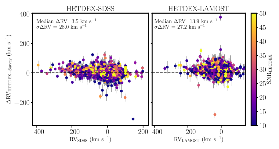
Figure 6: The difference RV determined using HETDEX spectra and those from the SEGUE as a function of the SEGUE RV (left panel). The same is shown on the right panel but for the LAMOST survey. Each star is color-coded by its SNR. The dotted black line in both represent when the HETDEX measured RV directly matches that of measured by the external survey. The median offset and dispersion of the difference in RV, $\Delta$RV, are noted in the diagram.

4.1 Radial Velocities

Our first goal was to measure HETDEX spectra RVs for stars with colors between 0.8 $<(BP-RP)<$ 2.0. The RVs were determined using the cross-correlation technique with a spectrum chosen from a grid of template spectra by identifying the best fitting synthetic spectrum. We refer the reader to section 3.1 for more details about the construction of the template grid, how the templates are matched to the observed spectra, and how the RVs were determined. The color range was selected in order to ensure that the $T_{\mathrm{eff}}$ of the star was not significantly hotter or cooler than the boundaries of the RV template grid. We were able to derive RVs, their uncertainties, and heliocentric corrections for 41,980 unique stars. However, many of these spectra have SNR $<$ 5 pixel^-1 and are therefore unlikely to yield high-quality RV estimates. If we we restrict our analysis to only those spectra with SNR $>$ 5 pixel^-1, we obtain 28,343 stars. Of these 28,343 stars, $\sim$602 ($\sim$2%) have RVs larger than 600 km s^-1. Visual inspection of the HETDEX spectra of these objects indicate that they are likely to be galaxies, so we remove any source with a measured RVs larger than 600 km s^-1 from our sample.

In order to validate the quality of the RVs determined from the HETDEX spectra (described in Section 2.2) and the cross-correlation technique (outlined in Section 3.1), we cross matched these stars against other large spectroscopic surveys at higher resolution (i.e., SEGUE and LAMOST). For the HETDEX-SEGUE cross match, which initially contained about 5,700 stars, we required that the SEGUE RV must be known with an uncertainty of less than 10 km s^-1 and a SEGUE-derived SNR $>$ 10. We also required the HETDEX-derived RV and SNR to be less than 600 km s^-1. These constrained reduced the HETDEX-SEGUE comparison to 1,456 stars. For the HETDEX-LAMOST comparison, which initially contained around 6,300 stars, we applied the same criteria as for the HETDEX-SEGUE comparison, which reduced the HETDEX-LAMOST external validation sample to 2,384 stars (see section 2.3 for more details).

Figure 6, presents the HETDEX RVs measured in this work compared with those a measured for the same stars in the HETDEX-SEGUE  (left panel) and the HETDEX-LAMOST (right panel) comparison samples. Each point represents an individual star and the points are color-coded by the HETDEX SNR. Figure 6 indicates that there is generally good agreement between the RVs measured by HETDEX and those by SEGUE with an systematic offset of +3.5 km s^-1 and a dispersion in the difference in RV, $\Delta$RV, of 28.0 km s^-1 (i.e., the RV measured by HETDEX is 3.5 km s^-1 larger than the ones from SEGUE). There is fair agreement between the RVs measured by HETDEX and those by LAMOST with a systematic offset of +13.9 km s^-1 and a dispersion in the $\Delta$RV of 27.2 km s^-1 (i.e., the RV measured by HETDEX is 13.9 km s^-1 larger than the ones from LAMOST). Additionally, there is a known difference of $\sim$ +9.1 km s^-1 difference in the RVs measured by LAMOST compared to those by SEGUE (whereby the SEGUE RVs are 9.1 km s^-1 larger than those from LAMOST) for the 66 stars that are in common between all three surveys and pass all quality criteria, indicating that the differences in the RV offset that we observe between the HETDEX-LAMOST (+13.9 km s^-1) and HETDEX-SEGUE (3.5 km s^-1) validation sets can be fully accounted for by the difference in the two RV scales. There is good agreement in the external precision (measured to be $\sim$28 km s^-1), to which we can measure RVs relative to the two independent validation sets. We note that these results are not significantly dependent on the median fraction of flux coverage of individual sources across fibers.

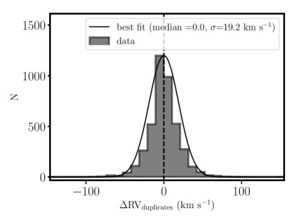
Figure 7: The distribution of the $\Delta$RV_duplicates for the $\sim$2000 stars with more than one epoch of spectra from HETDEX. The quantity $\Delta$RV_duplicates is the RV measured in all epoch subtracted from the median RV across all epochs for each star. The offset is consistent with zero while the dispersion, which is a measure of the internal precision, is $\sim$19 km s^-1(black line).

We can further test the measured RV precision in the HETDEX survey by quantifying the internal precision, i.e., by determining how consistent the HETDEX RVs are between stars with spectra obtained from multiple epochs. There are $\sim$2,000 unique stars which have multiple epochs of measured RVs. For each unique star with multiple spectra (and therefore multiple RV estimates), we obtain the difference in RV in each epoch and the median RV across all visits. We denote this quantity as $\Delta$RV_duplicates. The distribution of $\Delta$RV_duplicates can be found in Figure 7. There is an offset consistent with zero and a dispersion in $\Delta$RV_duplicates is 19.1 km s^-1. The dispersion in $\Delta$RV_duplicates represents a measure of the internal precision with which we can measure RVs from duplicate observations of the same (assumed to be single) stars.

Figure 8 shows how the internal precision, as measured by the dispersion in $\Delta$RV_duplicates, depends on SNR. As expected, the internal precision of RV measurements from HETDEX spectra degrades with decreasing SNR. The highest precision is for stars with SNR $>$ 30 pixel^-1 and the lowest is for those with SNR $<$ 10 pixel^-1. In the SNR regime that dominates the external validation sets, the internal (as measured by the duplicate spectra) and external precisions (as measure by the validation sets) are consistent. We assume that each star in the above analysis is a single star. If there were a significant fraction of unknown binaries, it would causes some of the scatter in the $\Delta$RV_duplicates.

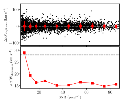
Figure 8: Top panel: The difference in the RVs measured between epochs and the median RV,$\Delta$RV_duplicates, for each star that has duplicate spectra as a function of the HETDEX SNR. The red squares represent the median and dispersion of $\Delta$RV_duplicates in 10 SNR bins. Bottom Panel: The dispersion in $\Delta$RV_duplicates, a measure of the internal RV precision, as a function of HETDEX SNR. The dispersion in $\Delta$RV_duplicates is $\sim$15 km s^-1 for the highest SNRs (SNR $>$ 30 pixel^-1), and rises to $\sim$29 km s^-1 for the lowest SNR (SNR $\sim$ 5 pixel^-1).

Taken together, these results indicate that we can conservatively measure RVs in HETDEX at the $\sim$28 km s^-1 level. We also find that the RVs measured with the HETDEX spectra most closely resemble those from SEGUE. However, SEGUE has an empirical correction on the order of $\sim$8 km s^-1 with respect to published values from star clusters (e.g., Lee et al., 2008a). Additionally, since RVs measured with LAMOST have a much lower zero-point correction (e.g., 0.02 km s^-1; Wang et al., 2019), we recommend subtracting 13.5 km s^-1 from the reported RVs to bring them onto the LAMOST RV scale.

With the RVs in hand, we correct all spectra to be in the rest-frame and move on to exploring the information content of the spectra through machine learning.

4.2 Finding Metal-Poor Stars in HETDEX with Machine Learning

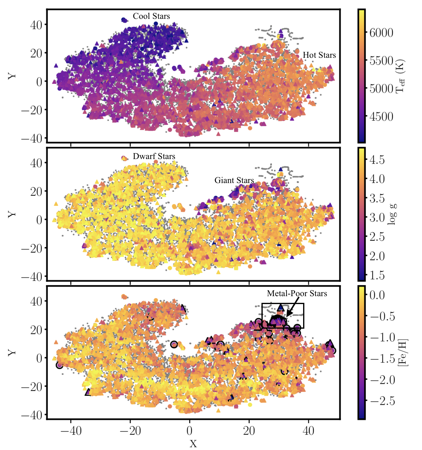
Figure 9: Two dimensional tSNE maps (in X and Y) of the HETDEX sample with RV measurements (small gray points). We highlight, by color-coding, any star with a known $T_{\mathrm{eff}}$ (top panel), log $g$ (middle panel), or [Fe/H] (bottom panel) from the SEGUE (colored circles) and LAMOST (colored triangles) surveys. In the bottom panel, metal-poor stars, with [Fe/H] $<-1.8$ dex, are highlighted with a black border around the symbol.

Using the RV corrected HETDEX spectra, we are able to potentially identify new metal-poor stars. To achieve this, we adopt the machine learning tSNE (section 3.2) with the HETDEX spectroscopic data. We input into tSNE the BMC normalized (see Section 2.2), RV corrected (see Sections 3.1 and 4.1) spectra for stars with 0.8 $<(BP-RP)<$ 2.0. The tSNE algorithm requires all spectra to be sampled on the same wavelength grid with no missing pixels (due to low coverage fractions, for example). To construct this dataset, we resampled the HETDEX spectra onto the same wavelength grid between 3640 $<\lambda<$ 5340 Å with 2 Å steps. Since we initially removed fluxes where the coverage fraction is less than 0.50 (see Section 2.2), we interpolated over the removed pixels during the resampling. To minimize the impact of this interpolation, we restricted ourselves to the $\sim$14,000 stars that have less than 5 pixels where the coverage fraction is less than 0.50 (i.e., we only replace as many as five pixels via interpolation). We initially configured tSNE with perplexity of 20 and a $\theta$ = 0.10 with 1000 maximum iterations. We examined both 2-D and 3-D projections of the dataset and found little benefit to higher dimensional projection.

Figure 9 shows the final projection of the high-D spectral dataset in 2-D. Each spectrum input into tSNe is represented by a closed gray circle in the figure; the final projection is color-coded by $T_{\mathrm{eff}}$ (top panel), log $g$ (middle panel), and [Fe/H] (bottom panel) where those quantitites are known by either SEGUE (colored circles) or LAMOST (colored triangles). This color-coding highlighted in this figure illustrates how the tSNE map can be used to identify regions where the spectra are similar (i.e., regions where the stars have similar atmospheric parameters). For example, in the final tSNE diagram, the coolest stars are in the upper corner left of center (i.e., X$\sim-10$, Y$\sim$+30) of the map (see top panel of Figure 9), the central part of the tSNE map contains the majority of the spectra, and the outer edges contain more peculiar classes of stars. Critically, in the bottom panel of Figure 9, demonstrates that the metal-poor stars largely clump up in the top right (i.e. X$\sim$25, Y$\sim$30) of the manifold, albeit with some spread. To help guide the eye, we place a black outline around any symbol with [Fe/H] $<-1.80$ dex. We also select a region where there are a high density of metal-poor stars (i.e. those with [Fe/H] $<$ –1.0 dex). This region contains 416 candidate metal-poor stars for further investigation.

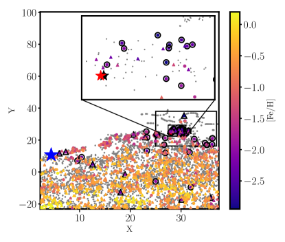
Figure 10: A zoom-in on the bottom panel of Fig. 9 inside the metal-poor selection box. The inset is a further expanded view. The red star symbol is a candidate metal-poor star (Gaia DR2 1593425105811347328), which has no known metallicity from any spectroscopic survey to date. The black star symbol is a known metal-poor star (Gaia DR2 2537923358055035648) from SEGUE. For comparision, the blue star symbol is a known more metal-rich star (Gaia DR2 2536562574976818816) with comparable $T_{\mathrm{eff}}$ and log $g$ values. The black star is almost entirely behind the red star because they were selected to be direct neighbors. Nearly all stars in the region with known metallicity have [Fe/H] $<-1.0$ dex.

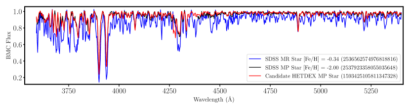
Figure 11: The HETDEX spectrum of a candidate metal-poor star (red line) identified from the tSNE map in Figure 9. For reference, also shown, as a black line, is a known metal-poor ([Fe/H] = $-2.00$) star from SEGUE that was closest to the candidate star in the tSNE diagram and a more metal-rich star (blue line), with [Fe/H] = $-0.34$ dex and a temperature within $\pm$200 K in $T_{\mathrm{eff}}$ and a log $g$ within $\pm$0.20 dex of the known metal-poor star.

Similar to Matijevič et al. (2017), Figure 9 demonstrates that it is possible to use HETDEX spectra to identify stars with [Fe/H] $<-1.0$ dex. To further illustrate this feature, in Figure 10 we select a known metal-poor star (Gaia DR2 2537923358055035648, black star symbol), which has a published metallicity of [Fe/H] = $-2.00$ dex from the SEGUE Stellar Parameter Pipeline (SSPP, Lee et al., 2008a, b; Allende Prieto et al., 2008; Smolinski et al., 2011). This figure identical to the bottom panel of Figure 9, however, we have enlarged the metal-poor selection box region. We also choose the closest point in tSNE space that does not have a known metallicity (Gaia DR2 1593425105811347328, red star symbol). The red and black stars representing the candidate and known metal-poor stars largely lie on top of each other in Figure 10 Since this star is closest to known metal-poor stars in the tSNE space, it is expected that its metallicity is an excellent metal-poor candidate. For reference, the location of a known metal-rich star (Gaia DR2 236562574976818816), with [Fe/H] = $-0.34$ dex, is also shown (blue star). This star was selected such that its SSPP $T_{\mathrm{eff}}$ was within $\pm$200 K and its SSPP log $g$ was within $\pm$0.20 dex of the known metal-poor star.

Figure 11 displays the RV corrected, BMC continuum normalized HETDEX spectrum of the known metal-poor star (black line), the metal-poor candidate star (red line), and the metal-rich comparison star (blue line). Figure 11 shows that the metal-poor candidate has absorption features that are much weaker than those of the known metal-rich star, and closely resemble the metal-poor candidate star. This indicates that the HETDEX spectra are of sufficient quality to find new metal-poor stars. The performance of tSNE is likely driven by the fact that $T_{\mathrm{eff}}$, [Fe/H]  and, to a lesser degree, log $g$ information is embedded in the spectra. This could be due to the advantageous wavelength regime, which includes various stellar parameter sensitive features (e.g., Ca H&K, Balmer lines).

We are currently obtaining observations of the brightest of these metal-poor candidate stars with higher resolution to accurately determine their metallicities and chemical abundances. The candidate metal-poor stars discussed here represent $\sim$3% of the total number of stars input into tSNE. Assuming the same percentage of metal-poor stars but an increase in sample size by $\sim$70%, one would naively predict HETDEX to contain thousands of metal-poor stars by its competition. Importantly, since there is no preselection to objects observed in HETDEX, the final metal-poor sample from HETDEX will enable us explore the stellar halo of the Milky Way with a relatively simple and quantifiable selection function.

5 Summary

The Hobby-Eberly Telescope Dark Energy Experiment (HETDEX) is an ongoing blind spectroscopic survey of more than 1 million Lyman-$\alpha$ emitting galaxies. However, in its search for these galaxies, it will observe 10⁵ stars. In this work, we focus on building the first catalogue of these stars and illustrate what can be done with them. We found stars in the HETDEX survey by cross matching more than $\sim$200 million HETDEX fiber spectra with the $\sim$1.6 billion Gaia point sources. This enabled us find 98,736 unique stars with HETDEX spectra. The spectra cover a broad range in the relatively faint magnitude regime of 10 $<G<$ 21 mag. Since HETDEX is an blind survey, it captures a wide range in stellar types from thousands of M-dwarfs to 100s of white dwarfs (see Figure 5). For the purposes of this work, we focused our attention on the late-type (largely FGK-type) stars by imposing a color cut of 0.8$<$ $(BP-RP)<$ 2.0. RVs were determined for these stars using cross-correlation with template spectra (Section 3.1). The results of that analysis show that RVs derived with HETDEX spectra are in good agreement with those measured by the SEGUE and LAMOST surveys. We find a median offset of 3.5 and 13.9 km s^-1 with the SEGUE and LAMOST surveys, respectively. Additionally, we demonstrate that the dispersion in the $\Delta$RV between HETDEX and these surveys is $\sim$30 km s^-1(Figures 6 and 7). Since Gaia will only be able to derive RVs for the brightest stars ($G<$14), for many of the faint stars in HETDEX  these results will be their only RV measurement.

We also attempted to determine whether the information content of the low-resolution spectra were enough to find metal-poor stars. To do this, we employed the tSNE machine learning algorithm which projects a high dimensional data set (i.e., the HETDEX spectra) onto a low dimensional manifold as a way to visualize the complexity of the data. This method has been employed in recent literature to search for metal-poor stars in moderate-resolution surveys (e.g. Matijevič et al., 2017), though here we apply it at the lowest spectral resolution to date. The results of the tSNE analysis can be found in Section 4.2. Using tSNE, we uncovered 416 new metal-poor candidate stars (Figures 9,  10 and 11), of which higher resolution spectroscopic followup is underway. The metal-poor stars identified here will be useful in constraining the formation of elements on the periodic table as well the early history of the Milky Way. Additionally, these results indicate that there is enough information embedded in the HETDEX spectra to not only derive $T_{\mathrm{eff}}$, and log $g$, but [Fe/H] as well.

This work represents the first attempt to extract and explore the stars observed by the HETDEX survey. The survey is ongoing and only $\sim$30% complete. Thus it is expected that there will by many more stars in the final HETDEX sample. In an upcoming paper, we plan to validate and chemically characterize the metal-poor candidate stars discovered here with higher resolution data, use tSNE to find other types of chemically peculiar stars (e.g. carbon enhanced stars), and attempt to measure the stellar atmospheric parameters directly from HETDEX spectra as we now know the information content is there (e.g. see Figure 9). Additionally, the results presented here provide an example of how low-resolution stellar spectra can be utilized in future surveys (e.g., in the upcoming Nancy Grace Roman Telescope Green et al., 2012) That combined with the blind nature of the survey will enable future stellar surveys with HETDEX to make a significant impact on Galactic Archaeology.

References

- Aguado et al. (2019) Aguado, D. S., Youakim, K., González Hernández, J. I., et al. 2019, MNRAS, 490, 2241, doi: 10.1093/mnras/stz2643
- Ahumada et al. (2019) Ahumada, R., Allende Prieto, C., Almeida, A., et al. 2019, arXiv e-prints, arXiv:1912.02905. https://arxiv.org/abs/1912.02905
- Allende Prieto et al. (2008) Allende Prieto, C., Sivarani, T., Beers, T. C., et al. 2008, AJ, 136, 2070, doi: 10.1088/0004-6256/136/5/2070
- Alvarez & Plez (1998) Alvarez, R., & Plez, B. 1998, A&A, 330, 1109
- Anders et al. (2018) Anders, F., Chiappini, C., Santiago, B. X., et al. 2018, A&A, 619, A125, doi: 10.1051/0004-6361/201833099
- Aoki et al. (2008) Aoki, W., Beers, T. C., Sivarani, T., et al. 2008, ApJ, 678, 1351, doi: 10.1086/533517
- Astraatmadja & Bailer-Jones (2016) Astraatmadja, T. L., & Bailer-Jones, C. A. L. 2016, ApJ, 832, 137, doi: 10.3847/0004-637X/832/2/137
- Astropy Collaboration et al. (2013) Astropy Collaboration, Robitaille, T. P., Tollerud, E. J., et al. 2013, A&A, 558, A33, doi: 10.1051/0004-6361/201322068
- Bailer-Jones (2015) Bailer-Jones, C. A. L. 2015, PASP, 127, 994, doi: 10.1086/683116
- Barnes & Hut (1986) Barnes, J., & Hut, P. 1986, Nature, 324, 446, doi: 10.1038/324446a0
- Beers & Christlieb (2005) Beers, T. C., & Christlieb, N. 2005, ARA&A, 43, 531, doi: 10.1146/annurev.astro.42.053102.134057
- Blanco-Cuaresma et al. (2014) Blanco-Cuaresma, S., Soubiran, C., Heiter, U., & Jofré, P. 2014, A&A, 569, A111, doi: 10.1051/0004-6361/201423945
- Boeche et al. (2018) Boeche, C., Smith, M. C., Grebel, E. K., et al. 2018, AJ, 155, 181, doi: 10.3847/1538-3881/aab5af
- Bromm & Larson (2004) Bromm, V., & Larson, R. B. 2004, ARA&A, 42, 79, doi: 10.1146/annurev.astro.42.053102.134034
- Buder et al. (2018) Buder, S., Asplund, M., Duong, L., et al. 2018, ArXiv e-prints. https://arxiv.org/abs/1804.06041
- Casagrande et al. (2019) Casagrande, L., Wolf, C., Mackey, A. D., et al. 2019, MNRAS, 482, 2770, doi: 10.1093/mnras/sty2878
- De Silva et al. (2015) De Silva, G. M., Freeman, K. C., Bland-Hawthorn, J., et al. 2015, MNRAS, 449, 2604, doi: 10.1093/mnras/stv327
- Frebel & Norris (2015) Frebel, A., & Norris, J. E. 2015, Annual Review of Astronomy and Astrophysics, 53, 631, doi: 10.1146/annurev-astro-082214-122423
- Gaia Collaboration et al. (2018) Gaia Collaboration, Brown, A. G. A., Vallenari, A., et al. 2018, ArXiv e-prints. https://arxiv.org/abs/1804.09365
- Gilmore et al. (2012) Gilmore, G., Randich, S., Asplund, M., et al. 2012, The Messenger, 147, 25
- Green et al. (2012) Green, J., Schechter, P., Baltay, C., et al. 2012, arXiv e-prints, arXiv:1208.4012. https://arxiv.org/abs/1208.4012
- Gustafsson et al. (2008) Gustafsson, B., Edvardsson, B., Eriksson, K., et al. 2008, A&A, 486, 951, doi: 10.1051/0004-6361:200809724
- Hawkins et al. (2014) Hawkins, K., Jofré, P., Gilmore, G., & Masseron, T. 2014, MNRAS, 445, 2575, doi: 10.1093/mnras/stu1910
- Hawkins et al. (2020) Hawkins, K., Lucey, M., Ting, Y.-S., et al. 2020, MNRAS, 492, 1164, doi: 10.1093/mnras/stz3132
- Hill (2014) Hill, G. J. 2014, Advanced Optical Technologies, 3, 265, doi: 10.1515/aot-2014-0019
- Hill & HETDEX Consortium (2016) Hill, G. J., & HETDEX Consortium. 2016, in Astronomical Society of the Pacific Conference Series, Vol. 507, Multi-Object Spectroscopy in the Next Decade: Big Questions, Large Surveys, and Wide Fields, ed. I. Skillen, M. Balcells, & S. Trager, 393
- Hill et al. (2008) Hill, G. J., Gebhardt, K., Komatsu, E., et al. 2008, in Astronomical Society of the Pacific Conference Series, Vol. 399, Panoramic Views of Galaxy Formation and Evolution, ed. T. Kodama, T. Yamada, & K. Aoki, 115. https://arxiv.org/abs/0806.0183
- Hill et al. (2018a) Hill, G. J., Drory, N., Good, J. M., et al. 2018a, in Society of Photo-Optical Instrumentation Engineers (SPIE) Conference Series, Vol. 10700, Proc. SPIE, 107000P, doi: 10.1117/12.2312350
- Hill et al. (2018b) Hill, G. J., Kelz, A., Lee, H., et al. 2018b, in Society of Photo-Optical Instrumentation Engineers (SPIE) Conference Series, Vol. 10702, Proc. SPIE, 107021K, doi: 10.1117/12.2314280
- Horne (1986) Horne, K. 1986, PASP, 98, 609, doi: 10.1086/131801
- Jofré et al. (2017) Jofré, P., Traven, G., Hawkins, K., et al. 2017, MNRAS, 472, 2517, doi: 10.1093/mnras/stx1877
- Karlsson et al. (2013) Karlsson, T., Bromm, V., & Bland-Hawthorn, J. 2013, Reviews of Modern Physics, 85, 809, doi: 10.1103/RevModPhys.85.809
- Kullback (1959) Kullback, S. 1959, Information Theory and Statistics (New York: Wiley)
- Lee et al. (2008a) Lee, Y. S., Beers, T. C., Sivarani, T., et al. 2008a, AJ, 136, 2022, doi: 10.1088/0004-6256/136/5/2022
- Lee et al. (2008b) —. 2008b, AJ, 136, 2050, doi: 10.1088/0004-6256/136/5/2050
- Lee et al. (2015) Lee, Y. S., Beers, T. C., Carlin, J. L., et al. 2015, AJ, 150, 187, doi: 10.1088/0004-6256/150/6/187
- Li et al. (2018) Li, H., Tan, K., & Zhao, G. 2018, ApJS, 238, 16, doi: 10.3847/1538-4365/aada4a
- Lucey et al. (2019) Lucey, M., Hawkins, K., Ness, M., et al. 2019, MNRAS, 488, 2283, doi: 10.1093/mnras/stz1847
- Luo et al. (2015) Luo, A.-L., Zhao, Y.-H., Zhao, G., et al. 2015, Research in Astronomy and Astrophysics, 15, 1095, doi: 10.1088/1674-4527/15/8/002
- Majewski et al. (2017) Majewski, S. R., Schiavon, R. P., Frinchaboy, P. M., et al. 2017, AJ, 154, 94, doi: 10.3847/1538-3881/aa784d
- Matijevič et al. (2017) Matijevič, G., Chiappini, C., Grebel, E. K., et al. 2017, A&A, 603, A19, doi: 10.1051/0004-6361/201730417
- Moffat (1969) Moffat, A. F. J. 1969, A&A, 3, 455
- Plez (2012) Plez, B. 2012, Turbospectrum: Code for spectral synthesis, Astrophysics Source Code Library. http://ascl.net/1205.004
- Ramsey et al. (1994) Ramsey, L. W., Sebring, T. A., & Sneden, C. A. 1994, in Society of Photo-Optical Instrumentation Engineers (SPIE) Conference Series, Vol. 2199, Proc. SPIE, ed. L. M. Stepp, 31–40, doi: 10.1117/12.176221
- Roederer et al. (2014) Roederer, I. U., Preston, G. W., Thompson, I. B., et al. 2014, AJ, 147, 136, doi: 10.1088/0004-6256/147/6/136
- Rogers et al. (2010) Rogers, B., Ferreras, I., Peletier, R., & Silk, J. 2010, MNRAS, 402, 447, doi: 10.1111/j.1365-2966.2009.15892.x
- Ruchti et al. (2010) Ruchti, G. R., Fulbright, J. P., Wyse, R. F. G., et al. 2010, ApJ, 721, L92, doi: 10.1088/2041-8205/721/2/L92
- Sakari et al. (2018) Sakari, C. M., Placco, V. M., Farrell, E. M., et al. 2018, ApJ, 868, 110, doi: 10.3847/1538-4357/aae9df
- Smolinski et al. (2011) Smolinski, J. P., Lee, Y. S., Beers, T. C., et al. 2011, AJ, 141, 89, doi: 10.1088/0004-6256/141/3/89
- Starkenburg et al. (2017) Starkenburg, E., Martin, N., Youakim, K., et al. 2017, MNRAS, 471, 2587, doi: 10.1093/mnras/stx1068
- Steinmetz et al. (2006) Steinmetz, M., Zwitter, T., Siebert, A., et al. 2006, AJ, 132, 1645, doi: 10.1086/506564
- Steinmetz et al. (2020) Steinmetz, M., Matijevič, G., Enke, H., et al. 2020, AJ, 160, 82, doi: 10.3847/1538-3881/ab9ab9
- Ting et al. (2017) Ting, Y.-S., Conroy, C., Rix, H.-W., & Cargile, P. 2017, ApJ, 843, 32, doi: 10.3847/1538-4357/aa7688
- van der Maaten (2014) van der Maaten, L. 2014, Journal of Machine Learning Research, 15, 3221. http://jmlr.org/papers/v15/vandermaaten14a.html
- van der Maaten & Hinton (2008) van der Maaten, L., & Hinton, G. 2008, Journal of Machine Learning Research, 9, 2579, doi: 10.3847/1538-3881/ab339a
- Virtanen et al. (2019) Virtanen, P., Gommers, R., Oliphant, T. E., et al. 2019, arXiv e-prints, arXiv:1907.10121. https://arxiv.org/abs/1907.10121
- Wang et al. (2019) Wang, R., Luo, A. L., Chen, J. J., et al. 2019, ApJS, 244, 27, doi: 10.3847/1538-4365/ab3cc0
- Xiang et al. (2019) Xiang, M., Ting, Y.-S., Rix, H.-W., et al. 2019, ApJS, 245, 34, doi: 10.3847/1538-4365/ab5364
- Xiang et al. (2017) Xiang, M.-S., Liu, X.-W., Yuan, H.-B., et al. 2017, MNRAS, 467, 1890, doi: 10.1093/mnras/stx129
- Xu et al. (2013) Xu, S.-Y., Zhang, H.-W., & Liu, X.-W. 2013, Research in Astronomy and Astrophysics, 13, 313, doi: 10.1088/1674-4527/13/3/006
- Yanny et al. (2009) Yanny, B., Rockosi, C., Newberg, H. J., et al. 2009, AJ, 137, 4377, doi: 10.1088/0004-6256/137/5/4377
- Yong et al. (2013) Yong, D., Norris, J. E., Bessell, M. S., et al. 2013, ApJ, 762, 26, doi: 10.1088/0004-637X/762/1/26
- York et al. (2000) York, D. G., Adelman, J., Anderson, Jr., J. E., et al. 2000, AJ, 120, 1579, doi: 10.1086/301513
- Zucker (2003) Zucker, S. 2003, MNRAS, 342, 1291, doi: 10.1046/j.1365-8711.2003.06633.x