Thermal buckling transition of crystalline membranes in a field

Abstract

Two dimensional crystalline membranes in isotropic embedding space exhibit a flat phase with anomalous elasticity, relevant e.g., for graphene. Here we study their thermal fluctuations in the absence of exact rotational invariance in the embedding space. An example is provided by a membrane in an orientational field, tuned to a critical buckling point by application of in-plane stresses. Through a detailed analysis, we show that the transition is in a new universality class. The self-consistent screening method predicts a second order transition, with modified anomalous elasticity exponents at criticality, while the RG suggests a weakly first order transition.

Introduction and background. Experimental realization of freely suspended graphene suspendGrapheneNature2007 and other exfoliated crystals, following the 2004 pioneering works of Geim and Novoselov Geim2004 , launched extensive research in electronic and mechanical properties of two-dimensional crystalline membranesGeimMacDonald ; reviewRMPGraphene . This led to a renaissance in the statistical mechanics of fluctuating elastic membranes, first studied in the context of soft and biological matter three decades ago NP ; AL ; CrumplingBucklingGuitter ; GDLP ; LRprl ; LRrapid ; GuitterMC ; Jerusalem ; Bensimon ; RTtubule ; LRReview . Theoretical interest is also motivated by the opportunity to explore the nontrivial and rich interplay between field theory and geometry Jerusalem .

The most striking prediction is the existence of a low-temperature stable “flat” phase of a tensionless crystalline membrane NP , that spontaneously breaks rotational symmetry of the embedding space. This is in stark contrast to canonical two-dimensional field theories for which the Hohenberg-Mermin-Wagner theoremsHohenberg ; MerminWagner ; Coleman , preclude spontaneous breaking of a continuous symmetry in two dimensions.

In such elastic membranes, in a spectacular phenomenon of order-from-disorder, thermal fluctuations instead stiffen the long-wavelength ($k^{-1}$) bending rigidity $\kappa_{0}\rightarrow\kappa_{0}k^{-\eta}$, $\eta>0$, via a universal power-law “corrugation” effect, with membrane roughness scaling as $h_{\text{r}ms}\sim L^{\zeta}$, with $\zeta=(4-D-\eta)/2$NP ; Jerusalem , where $D$ is membrane’s internal dimension, with $D=2$ for the physical case. The resulting anomalous elasticity is characterized by universal exponents, $\eta,\zeta$ and $\eta_{u}=4-D-2\eta$ determined exactly by the underlying rotational invariance, with a scale dependent Young modulus $K_{0}\to K_{0}q^{\eta_{u}}$. This was predicted, together with the values of the exponents, by a variety of complementary methods NP ; AL ; GDLP ; LRprl ; LRReview . It was verified in numerical simulations simulationsGraphene and continues to be explored experimentally experimentElasticModuli .

Most theoretical studies to-date have focused on stress-free fluctuating membranes in an isotropic embedding environment NP ; AL ; GDLP ; LRprl ; LRrapid ; RTtubule ; LRReview ; Gazit ; MirlinPoisson1 ; Mouhanna1 ; MouhannaCrumpling ; MouhannaTwoLoopFlat , as appropriate for e.g., soft matter realizations of a membrane in an isotropic fluid (though see interesting generalizations for spherical shellsPouloseNelsonPNAS2012 ; Kosmrlj ). However, many experiments on graphene and other solid-state membranes (even some suspended ones) may be subjected to embedding space anisotropy and/or external stresses due to the presence of a substrate GuineaPuddlesSubstrate ; GuineaPinningSubstrate ; GuineaPLDSubstrate , clampingBowick2020Buckling ; Bowick2017Clamped ; MorshedifardKosmrljBuckling2021 , or electric and magnetic fieldsBoothGeimNanoLett2008 ; BleesMcEuenKirigamiNature2015 . Orientational fields could also be imposed by suspending the membrane in a nematic solventLehenyDiskNematic . This was realized in Barium hexaferrite platelets by the Ljubljana groupnematicSheetsCopic ; nematicSheetsSmalyukh ; grapheneNematicClark showing that they form a ferromagnetic nematic, with membranes’ normals aligning with the nematic director and manipulatable by an external magnetic field. It is interesting to consider for instance the case of an uniaxial easy axis field tending to order the membrane’s normal, and/or the application of a boundary stress $\sigma$. In all previous theoretical descriptions, the rotational invariance in the embedding space was assumed and the response found to be controlled by the thermal tensionless membrane fixed pointAL . The case of weak field or stresses is treated by simply introducing a cutoff for the isotropic critical fluctuations, beyond a large scale $\xi\sim(\kappa/\sigma)^{\nu}$, that diverges with a vanishing $\sigma$, where $\nu$ is a universal exponent that we compute below. Such perturbations then lead to an anomalous response, that in the context of tension predicts a non-Hookean stress-strain relation $\varepsilon\sim\sigma^{\alpha}$, with $\alpha=(D-2+\eta)/(2-\eta)=_{D=2}\eta/(2-\eta)$. CrumplingBucklingGuitter ; GDLP ; ML ; RTtubule ; LRReview ; Mirlin ; MirlinPoisson1 ; MirlinPoisson2 .

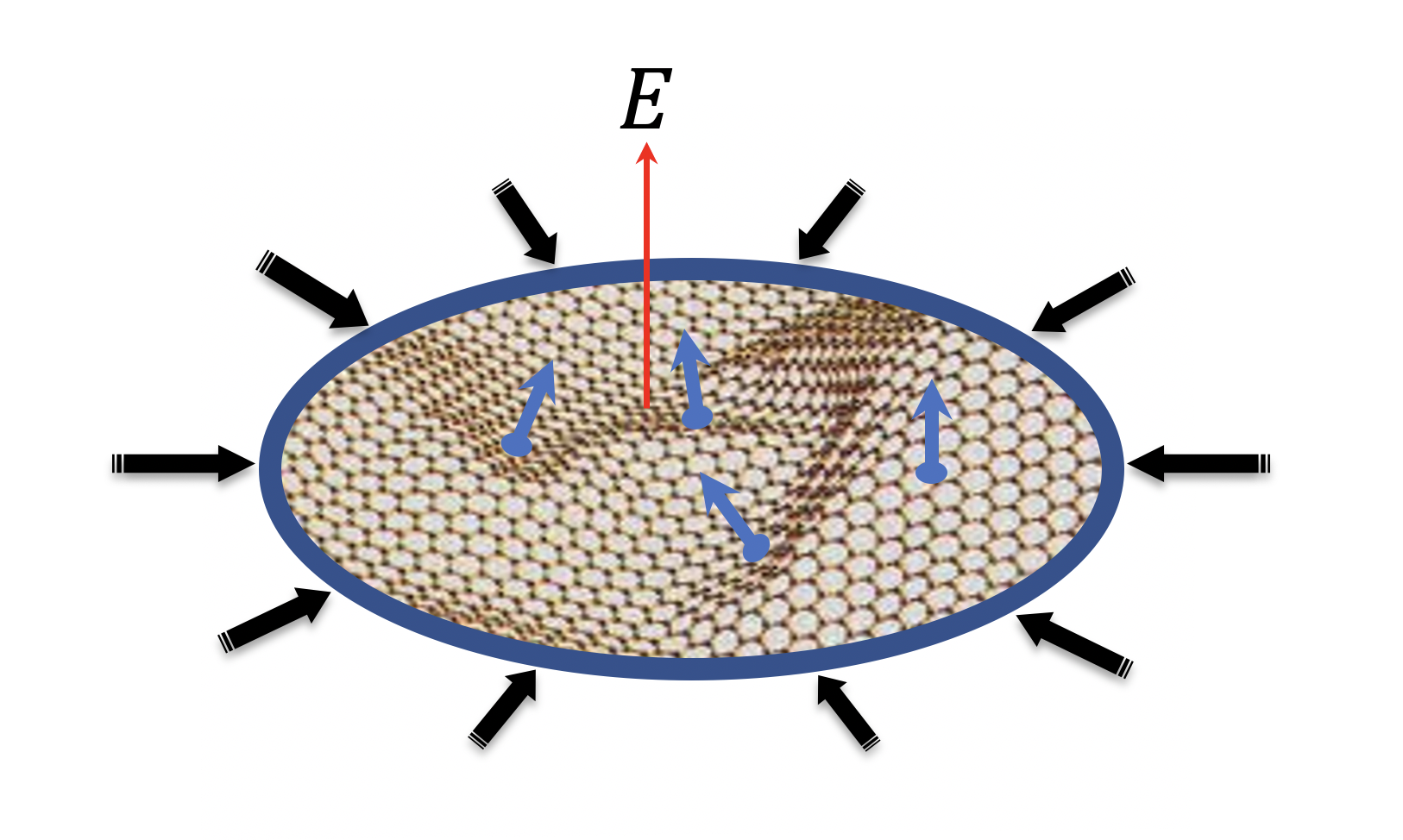
Figure 1: A schematic illustration of a critical membrane tuned to a buckling transition, subjected to an external in-plane isotropic stress $\sigma_{ij}=\frac{1}{2}\sigma\delta_{ij}$, stabilized and balanced by an external field $\vec{E}$, which tends to align the normals (blue vectors).

In this Letter we describe such experimental geometries, illustrated in Fig.1, where the imposed stress and anisotropy lead to qualitatively richer and universal buckling phenomenology. Generic buckling is a complex out-of-plane instability of a sheet subjected to compression, that results in a strongly distorted, non-perturbative state. Recently, there has been significant interest and progress in the study of isotropic buckling, with focus on effects of thermal fluctuations on the classical problem of Euler buckling, stabilized only by finite size effects.MorshedifardKosmrljBuckling2021 Instead, here we focus on a gentler, continuous anisotropic form of this transition, where the instability is controlled by a stabilizing external field. Specifically, we consider an externally oriented membrane tuned to a buckling transition by a compressional boundary stress applied within the plane explicitly selected by the orientational field gentle . The compressive stress can be tuned to a critical value, $\sigma_{c}$ to cancel out at quadratic order the (embedding-space) rotational symmetry breaking fields. Our key observation is that at this new buckling critical point (to which the isotropic flat membrane critical pointAL is unstable), although at harmonic order the membrane appears to be rotationally invariant and stress-free, thus exhibiting strong thermal fluctuations, it admits new important elastic nonlinearities that are not rotationally invariant. These lead to a critical membrane, tuned to the buckling point, that is, thus qualitatively distinct from the conventional tensionless membranefootnote1 .

Results. Subjecting a crystalline membrane to a lateral compressive isotropic boundary stress $\sigma$, tuned to a critical tensionless buckling point $\sigma_{c}$ and stabilized by an orienting field, we find a new buckling universality class, distinct from the isotropic tensionless membraneNP ; AL ; GDLP ; LRprl ; LRReview . We propose a model based on symmetry arguments, supported by more detailed considerations. We use two complementary approaches to analyze the properties of the resulting critical state. The first is the self-consistent screening approximation (SCSA) which was found to provide an accurate description for the isotropic case LRprl ; LRReview . Thermal fluctuations and elastic nonlinearities at the buckling transition lead to a universal anomalous elasticity with exponent

$$\eta^{\rm anis} = 0.754,$$ (1)

characterizing the divergence of the effective length-scale dependent bending rigidity $\kappa(k)\sim k^{-\eta}$. The in-plane elastic moduli remain finite at the critical point, i.e., $\eta_{u}^{\rm anis}=0$ footnote2 . This is despite the fact that the five eigen-couplings $w_{i}(q)\sim q^{4-D-2\eta}$ renormalize nontrivially, vanishing in the long wavelength limit. This is at variance with the tensionless isotropic membrane for which SCSA predicts universal exponents $\eta\approx 0.821$, $\eta_{u}\approx 0.358$ LRprl . The corresponding roughness $h_{\text{rms}}\sim L^{\zeta}$ of the critically buckled membrane is characterized by a universal roughness exponent

$$\zeta^{\rm anis}=0.623,$$ (2)

and it is thus rougher than a tensionless isotropic membrane, with a roughness exponent $\zeta\approx 0.59$ LRprl .

We complement this SCSA calculation by an RG analysis in an expansion in $\epsilon=4-D$. It confirms the instability of the standard anomalous elasticity fixed point of the isotropic, tensionless membrane, under breaking of the embedding space rotational symmetry. Let us recall that for the isotropic membrane the elastic nonlinearities destabilize the harmonic theory (i.e., the Gaussian fixed point) beyond the length scale $\xi^{\rm iso}_{\rm NL}\sim(\frac{\kappa^{2}}{TK_{0}})^{\frac{1}{4-D}}$. If the anisotropy perturbation is very weak, e.g., $w\sim\mu_{1,2},\lambda_{1,2}\ll K_{0}$ (see below for definitions of these anisotropy parameters), the membrane still experiences the standard isotropic anomalous elasticity up to scales $\xi^{\rm iso}_{\rm NL}$, crossing over to the new anisotropic critical behavior beyond the crossover length

$$\xi^{\rm anis}_{NL}=\xi^{\rm iso}_{\rm NL}\left(\frac{K_{0}}{w}\right)^{1/\rho}\ ,\quad\rho=\frac{\epsilon d_{c}}{d_{c}+24}+O(\epsilon^{2}),$$ (3)

where $\rho$ is the crossover exponent obtained from linearization of the RG flow around the isotropic fixed point. If the anisotropy perturbation is stronger, the thermal fluctuations and elastic nonlinearities directly destabilize the harmonic theory at scales of order $\xi^{\rm iso}_{\rm NL}$. Beyond these scales, the RG flows to a new stable buckling critical point, which, within the $\epsilon$-expansion, is however accessible only for space codimension $d_{c}=d-D>219$, analogous to the crumpling transition found by Paczuski, et al.PKN . For the physical case, $d_{c}=1$, we interpret the resulting runaway flows as a weakly first order transition, as for the standard crumpling transition. We note that the SCSA is exact for the large $d_{c}$ limit, and confirm that the two methods match in their common regime of validity.

Model of anisotropic membrane buckling. The coordinates of the atoms in the $d$-dimensional embedding space are denoted $\vec{r}({\bf x})\in\mathbb{R}^{d}$, with the atoms labeled by their position ${\bf x}\in\mathbb{R}^{D}$ in the internal space. For graphene $D=2$, and atoms span a triangular lattice, described here in the continuum limit. The deformations with respect to the flat sheet are described by $D$ phonon fields $u_{\alpha}({\bf x})$, and $d_{c}=d-D$ height fields $\vec{h}\in\mathbb{R}^{d_{c}}$ (orthogonal to the $\vec{e}_{\alpha}$) as $\vec{r}({\bf x})=(x_{\alpha}+u_{\alpha}({\bf x}))\vec{e}_{\alpha}+\vec{h}({\bf x})$, where the $\vec{e}_{\alpha}$ are a set of $D$ orthonormal vectors. While the physical case corresponds to $d=3$ and $d_{c}=1$, it is useful to study the theory for a general $d_{c}$. The nonlinear strain tensor measures the deformation of the induced metric relative to the preferred flat metric, $u_{\alpha\beta}=\frac{1}{2}(\partial_{\alpha}\vec{r}\cdot\partial_{\beta}\vec{r}-\delta_{\alpha\beta})\simeq\frac{1}{2}(\partial_{\alpha}u_{\beta}+\partial_{\beta}u_{\alpha}+\partial_{\alpha}\vec{h}\cdot\partial_{\beta}\vec{h})$ to the accuracy needed here, with the $O((\partial u)^{2})$ phonon nonlinearities irrelevant and therefore neglected (see below). The tensor $u_{\alpha\beta}$ encodes full rotational invariance in the embedding space, its approximate form being invariant under infinitesimal rotations by $\theta$, i.e., the $O(\theta^{2})$ term vanishes under the (apparent) distortion $u_{1}=x_{1}(\cos\theta-1)$, $h_{1}=x_{1}\sin\theta$, which corresponds to a rigid rotation, with the corresponding vanishing of the exact strain tensor.

Here we build on the model of a rotationally invariant tensionless membrane. Its Hamiltonian is the sum of curvature energy and in-plane stretching energy

$${\cal F}_{1}[\vec{h},u_{\alpha}]=\int d^{D}x\,\left[\frac{\kappa}{2}(\partial^{2}\vec{h})^{2}+\tau u_{\alpha\alpha}+\mu(u_{\alpha\beta})^{2}+\frac{\lambda}{2}(u_{\alpha\alpha})^{2}\right]$$ (4)

where $\kappa$ is the bending modulus, $\lambda,\mu$ the in-plane Lamé elastic constants. The parameter $\tau$ controls the preferred extension of the membrane in the $\vec{e}_{\alpha}$ plane.

Based on symmetry considerations, complemented by a model-building derivation (presented at the end of the paper), external orientational and boundary stresses introduce new relevant elastic nonlinearities, with five new independent couplings, that by symmetry lead to a modified effective Hamiltonian ${\cal F}={\cal F}_{1}+{\cal F}_{2}$, where ${\cal F}_{2}$ breaks rotational invariance in the embedding space,

$${\cal F}_{2}[\vec{h},u_{\alpha}]=\int d^{D}x\,\bigg{(}\frac{\gamma}{2}(\partial_{\alpha}\vec{h})^{2}$$ (5)

$$+\frac{\lambda_{1}}{2}\partial_{\alpha}u_{\alpha}(\partial_{\beta}\vec{h})^{2}+\frac{\lambda_{2}}{8}[(\partial_{\alpha}\vec{h})^{2}]^{2}$$

$$+\mu_{1}\partial_{\alpha}u_{\beta}(\partial_{\alpha}\vec{h}\cdot\partial_{\beta}\vec{h})+\frac{\mu_{2}}{4}[\partial_{\alpha}\vec{h}\cdot\partial_{\beta}\vec{h}]^{2}\bigg{)},$$

retaining in-plane isotropy and the $h\to-h$ invariance as a feature of our geometry, preserving the equivalence between the two sides of the membrane.

We now study the membrane with parameters tuned to the thermal buckling critical point defined by the renormalized $\gamma_{R}=0$. Integrating over the in-plane phonon modes $u_{\alpha}$ and, rescaling for convenience all elastic constants by $1/d_{c}$, we obtain an effective Hamiltonian for the height field,

$${\cal F}[\vec{h}]=\int d^{D}x\,[\frac{\kappa}{2}(\partial^{2}\vec{h})^{2}+\frac{\gamma}{2}(\partial_{\alpha}\vec{h})^{2}]+\frac{1}{4d_{c}}\int d^{D}x\,d^{D}y$$

$$\,\,\,\,\times\partial_{\alpha}\vec{h}({\bf x})\cdot\partial_{\beta}\vec{h}({\bf x})\,R_{\alpha\beta,\gamma\delta}({\bf x}-{\bf y})\,\partial_{\gamma}\vec{h}({\bf y})\cdot\partial_{\delta}\vec{h}({\bf y}),$$ (6)

with a non-local quartic tensorial interaction, which in Fourier space is given byfootnoteFisherShankaNelsonRG

$$R_{\alpha\beta,\gamma\delta}({\bf q})=\sum_{i=1}^{5}w_{i}\,(W_{i})_{\alpha\beta,\gamma\delta}({\bf q}).$$ (7)

The $W_{i}$ are five projectors in the space of four index tensors, equal to bilinear combinations of longitudinal $P^{L}_{\alpha\beta}({\bf q})=q_{\alpha}q_{\beta}/q^{2}$ and transverse $P^{T}({\bf q})=\delta_{\alpha\beta}-P^{L}_{\alpha\beta}({\bf q})$ projectors on the wave vector ${\bf q}$. The five ”bare couplings” $w_{i}$ are given in the Supplementary Material (SM) SM in terms of the bare elastic moduli in (4) and (5), together with the basis tensors $W_{i}$. footnote3 The important features are the following. When rotational symmetry breaking is absent, $\gamma=0$, $\mu_{1}=\mu_{2}=\lambda_{1}=\lambda_{2}=0$, the couplings $w_{2},w_{4},w_{5}$ vanish and

$$w_{1}=\mu\quad,\quad w_{3}=\mu+(D-1)\frac{\mu\lambda}{\lambda+2\mu},$$ (8)

leading to (the ${\bf q}$ dependence suppressed)

$$R_{\alpha\beta,\gamma\delta}=(w_{3}-w_{1})P_{\alpha\beta}^{T}P_{\gamma\delta}^{T}+w_{1}\frac{1}{2}(P_{\alpha\gamma}^{T}P_{\beta\delta}^{T}+P_{\alpha\delta}^{T}P_{\beta\gamma}^{T}),$$ (9)

which is the usual quartic coupling associated to ${\cal F}_{1}$. When $\lambda_{1}$ and $\lambda_{2}$ are turned on, while $\mu_{1}=\mu_{2}=0$, all $w_{i}$ are nonzero except $w_{2}=0$. Finally, when all couplings in ${\cal F}_{2}$ are nonzero, all $w_{i}$ are nonzero.

SCSA analysis. The form (Thermal buckling transition of crystalline membranes in a field) is suitable to apply the SCSA method, which is exact in the limit of large $d_{c}$. The calculation is performed in the SM SM and parallels the one in Section IV. A of LRReview . Consider the two point correlation of the height field in Fourier space, $\langle h^{i}({\bf k})h^{j}({\bf k}^{\prime})\rangle={\cal G}(k)(2\pi)^{d}\delta^{d}({\bf k}+{\bf k}^{\prime})\delta_{ij}$. If we neglect the quartic nonlinearities in (Thermal buckling transition of crystalline membranes in a field) we find ${\cal G}(k)=G(k)=1/(\gamma k^{2}+\kappa k^{4})$. The nonlinearities lead to a nonzero self-energy $\Sigma(k)={\cal G}(k)^{-1}-\gamma k^{2}-\kappa k^{4}$. Together with the renormalized interaction tensor, $\tilde{R}({\bf q})$, it satisfies the SCSA equations

$$\Sigma(k)=\frac{2}{d_{c}}\int_{q}k_{\alpha}(k_{\beta}-q_{\beta})(k_{\gamma}-q_{\gamma})k_{\delta}\tilde{R}_{\alpha\beta,\gamma\delta}({\bf q}){\cal G}({\bf k}-{\bf q})$$

(10)

$$\tilde{R}({\bf q})=R({\bf q})-R({\bf q})\Pi({\bf q})\tilde{R}({\bf q})$$ (11)

where $\Pi({\bf q})$ encodes the screening of the in-plane elasticity by out of plane fluctuations

$$\Pi_{\alpha\beta,\gamma\delta}({\bf q})=\frac{1}{4}\int_{p}v_{\alpha\beta}({\bf q},{\bf q}-{\bf p})v_{\gamma\delta}({\bf q},{\bf q}-{\bf p}){\cal G}({\bf p}){\cal G}({\bf q}-{\bf p})$$ (12)

and $v_{\alpha\beta}({\bf p},{\bf p}^{\prime})=p_{\alpha}p^{\prime}_{\beta}+p^{\prime}_{\alpha}p_{\beta}$. One can decompose $\Pi({\bf q})=\sum_{i=1}^{5}\pi_{i}(q)W_{i}({\bf q})$ and $\tilde{R}({\bf q})=\sum_{i=1}^{5}\tilde{w}_{i}(q)W_{i}({\bf q})$, where $\tilde{w}_{i}(q)$ are the momentum dependent renormalized couplings. Looking for a solution which behaves at small $k$ as ${\cal G}(k)\simeq Z_{\kappa}^{-1}/k^{4-\eta}$, and evaluating the integrals $\pi_{i}(q)$ SM one finds that they diverge at small $q$ as $\pi_{i}(q)\simeq Z_{\kappa}^{-2}a_{i}q^{-(4-D-2\eta)}$ where $a_{i}=a_{i}(\eta,D)$. From (11) we find that the renormalized couplings are softened at small $q$ as $\tilde{w}_{i}(q)\propto Z_{\kappa}^{2}c_{i}q^{\eta_{u}}$, with $\eta_{u}=4-D-2\eta$ and $c_{i}=1/a_{i}$ for $i=1,2$ and

$$\begin{pmatrix}c_{3}&c_{4}\\ c_{4}&c_{5}\end{pmatrix}\simeq\begin{pmatrix}a_{3}&a_{4}\\ a_{4}&a_{5}\end{pmatrix}^{-1}$$ (13)

Inserting this into the self-energy equation (Thermal buckling transition of crystalline membranes in a field) and performing the integrals we find that the factors of $Z_{\kappa}$ cancel and the self-consistent equation, which implicitly determines $\eta$ as a function of $D,d_{c}$ is given by

$$\frac{d_{c}}{2}=\sum_{i=1,2}{b_{i}\over a_{i}}+{b_{3}a_{5}-b_{4}a_{4}+b_{5}a_{3}\over{a_{3}a_{5}-a_{4}^{2}}},$$ (14)

where $b_{i}=b_{i}(\eta,D)$ are self-energy integrals, given with the $a_{i}(\eta,D)$ in the SM. Note that here we have considered the case where all bare couplings $w_{i}$ are nonzero. For a physical membrane, $D=2$, (14) reduces to finding the root of a cubic equation

$$d_{c}=\frac{24(\eta-1)^{2}(2\eta+1)}{(\eta-4)\eta(2\eta-3)}.$$ (15)

For $d_{c}=1$ we obtain our main result (1). For large $d_{c}$ we find $\eta=2/d_{c}+O(1/d_{c}^{2})$. The roughness of a size $L$ membrane is characterized by $h_{\rm rms}=\langle h^{2}\rangle^{1/2}\simeq L^{\zeta}$ where $\zeta=(4-D-\eta)/2$. Hence for $d_{c}=1$ we find $\zeta=0.623$.

One can define renormalized amplitude ratio as

$$\lim_{q\to 0}\frac{\tilde{w}_{i}(q)}{\tilde{w}_{j}(q)}=\frac{c_{i}}{c_{j}}$$ (16)

for any pair $(i,j)$ such that the bare couplings $w_{i},w_{j}$ are nonzero. Near $D=4$ we find that these renormalized couplings take values such that the interaction energy becomes $\frac{v_{1}}{2}[(\partial_{\alpha}\vec{h})^{2}]^{2}+v_{2}(\partial_{\alpha}\vec{h}\cdot\partial_{\beta}\vec{h})^{2}$, i.e., local in the fields $\partial_{\alpha}\vec{h}$. This property however does not hold for $D<4$, e.g., one finds $c_{2}/c_{1}=(D+\eta-2)/(2-\eta)$ instead of unity for $D=4$, $\eta=0$. Thus the critical point requires a fully non-local five coupling description. The $c_{i}$ are given in SM . In the physical case of $D=2$ and $d_{c}$=1 we find

$$c_{i}=\{\frac{1}{2},0.302,0.338,-0.029,0.173\},$$ (17)

and the universal $\lambda/\mu=-0.978$ and the Poisson ratio (not to be confused with external stress),

$$\sigma^{\rm anis}=-0.968,$$ (18)

to be contrasted with $\sigma=-1/3$ for an isotropic tensionless membraneLRprl ; LRReview

There are other fixed points that lie in the invariant subspaces of the SCSA equations. The rotationally invariant membrane corresponds to bare couplings $w_{2}=w_{4}=w_{5}=0$. The corresponding renormalized couplings also vanish, which amounts to $b_{2}=b_{4}=b_{5}=0$ in (14), leading to

$$\frac{d_{c}}{2}=\frac{b_{1}}{a_{1}}+{b_{3}\over{a_{3}}},$$ (19)

which is precisely the SCSA equation for the anomalous flat phase of the isotropic membrane, leading for $D=2$ to $\eta=\frac{4}{d_{c}+\sqrt{16-2d_{c}+d_{c}^{2}}}$, and $\eta\simeq 0.821$, $\zeta=0.590$ for $d_{c}=1$ LRprl ; LRReview . Near $D=4$ one recovers $\eta=\frac{12}{d_{c}+24}\epsilon+O(\epsilon^{2})$ from the Aronovitz-Lubensky’s $\epsilon$-expansionAL . Another fixed manifold is $w_{2}=0$, corresponding to a choice of bare couplings so that $(\mu+\mu_{1})^{2}=\mu(\mu+\mu_{2})$, which includes the choice $\mu_{1}=\mu_{2}=0$, leading to $\tilde{w}_{2}(q)=0$ and

$$\frac{d_{c}}{2}={b_{1}\over a_{1}}+{b_{3}a_{5}-b_{4}a_{4}+b_{5}a_{3}\over{a_{3}a_{5}-a_{4}^{2}}}.$$ (20)

This leads to yet another fixed point with slightly different exponents. For $D=2$ and $d_{c}=1$ we find $\eta=0.854$ and $\zeta=0.573$. Near $D=4$ we find $\eta=\frac{18}{d_{c}+36}\epsilon+O(\epsilon^{2})$. Universal amplitude ratios have $c_{2}=0$.

RG analysis. As a nontrivial check and for further insight, we have complemented this SCSA calculation and results using an RG analysis, controlled by an $\epsilon=4-D$ expansion near $D=4$. We have calculated the one-loop corrections to the Hamiltonian (Thermal buckling transition of crystalline membranes in a field) and obtained the RG equations for the five dimensionless couplings $\hat{w}_{i}=w_{i}/\kappa^{2}C_{4}\Lambda_{\ell}^{-\epsilon}$ of the form $\partial_{\ell}\hat{w}_{i}=\epsilon\hat{w}_{i}+a_{ijk}\hat{w}_{j}\hat{w}_{k}$, where the $a_{ijk}$ and details of the calculation are given in SM . The anomalous dimension of the out-of-plane height field $h$ defines the exponent $\eta$ given by

$$\eta=\frac{1}{12}\left(10\hat{w}_{1}-18\hat{w}_{2}+5\hat{w}_{3}+3\hat{w}_{5}-6\hat{w}_{44}\right),$$ (21)

with $\hat{w}_{44}=\sqrt{3}\hat{w}_{4}$, and evaluated at the fixed point of interest $\hat{w}_{i}^{*}$ (see below). The anomalous dimension of the phonon field is given by

$$\eta_{u}=\frac{1}{12}(\hat{w}_{1}-\hat{w}_{2}).$$ (22)

The isotropic membrane corresponds to the space $\hat{w}_{2}=\hat{w}_{4}=\hat{w}_{5}=0$, which is preserved by the RG flow and along which

$$\partial_{\ell}\hat{w}_{1}=-\frac{1}{12}\hat{w}_{1}\left((d+20)\hat{w}_{1}+10\hat{w}_{3}\right),$$ (23)

$$\partial_{\ell}\hat{w}_{3}=-\frac{5}{24}\hat{w}_{3}\left((d+4)\hat{w}_{3}+8\hat{w}_{1}\right).$$ (24)

The isotropic membrane fixed point is $\hat{w}^{*}_{1}=\frac{12\epsilon}{d+24}$, $\hat{w}^{*}_{3}=\frac{24\epsilon}{5(d+24)}$, corresponding to $\hat{\mu}^{*}=\frac{12\epsilon}{24+d}$, $\hat{\lambda}^{*}=\frac{-4\epsilon}{24+d}$ AL . Diagonalizing the RG flow for $\hat{w}_{i}=\hat{w}_{i}^{*}+\delta\hat{w}_{i}$ around this fixed point in the larger space of five couplings shows that, in addition to the two negative eigenvalues $-1$ and $-\frac{d_{c}}{d_{c}+24}$ within the plane $\delta\hat{w}_{1,3}$ of the isotropic membrane, (i) there is a marginal direction mixing $\delta\hat{w}_{1,3,4}$ (eigenvalue $0$) (ii) there are two unstable directions with eigenvalues $\frac{d_{c}}{d_{c}+24}$ with $\delta w_{2,5}$ nonzero (in the large $d_{c}$ limit this eigenspace is purely along $\delta w_{2,5}$). Hence, consistent with the SCSA findings, the isotropic membrane fixed point is unstable to anisotropy of the orientational field and external boundary stress.

To determine where the general flow goes we searched for attractive fixed points of the RG equations. We found one such fixed point in the subspace of couplings $\hat{w}_{i}$ at which, the interaction energy is fully local in the gradients $\partial_{\alpha}\vec{h}$ and parameterized by two couplings $v_{1},v_{2}$ as defined above. This subspace is preserved by the RG and also arises in the study of the crumpling transition. In fact the RG flow within this subspace is identical to the one obtained in PKN with $d$ replaced by $d_{c}$. It admits a stable FP for $d_{c}>219$. Here we demonstrated that this FP is fully attractive in the space of the five couplings. Hence the RG approach is consistent, around $D=4$, with the SCSA (which is exact for large $d_{c}$ and any $D$), predicting a new fixed point for membrane in anisotropic embedding space. For the physical membrane $D=2$ and $d_{c}=1$, while the SCSA predicts this new ”anisotropic buckling transition” to be continuous, the RG, if extrapolated from $D=4$, suggests a weakly first order transition, as argued for the crumpling transition PKN ; Mouhanna1 ; MouhannaCrumpling .

To reach the new anisotropic buckling critical point requires tuning $\gamma=\gamma_{c}$, so that $\gamma_{R}=0$. Slightly away from criticality the correlation length is long but finite, $\xi\sim|\delta\gamma|^{-\nu}$, diverging with a vanishing $\delta\gamma=\gamma-\gamma_{c}$. Linearizing the RG flow around the fixed point yields $\delta\gamma(L)\sim\delta\gamma L^{\theta}$, where $\theta=-\frac{\epsilon}{d_{c}}(1-\frac{66}{d_{c}}+O(\frac{1}{d_{c}^{2}}))$, see the SM SM . By balancing $\kappa(\xi)\xi^{-4}\sim\delta\gamma(\xi)\xi^{-2}$ and using that $\kappa(\xi)\sim\xi^{\eta}$ we obtain the correlation length exponent as $\nu=1/(2+\theta-\eta)$.

Model development. Until now we argued for the model (4,5) based on symmetry considerations. Here, as illustrated in Fig.1, we develop an explicit model of a membrane undergoing buckling in the absence of rotational invariance in the embedding space. We consider an elastic membrane in an external field $\vec{E}$ (taken along the z-axis) that aligns the membrane’s normal $\hat{n}$ along the field. We thus expect the energy density to be a monotonic function of $\hat{n}\cdot\vec{E}$, namely of the small tilt angle $\theta$,

$${\cal H}_{\text{o}rient} = \frac{\alpha_{1}}{2}\theta^{2}+\frac{\tilde{\alpha}_{2}}{4}\theta^{4}+\ldots,$$ (25)

with $\alpha_{1}>0$, $\tilde{\alpha}_{2}>0$. Combining this orientational field energy with the Hamiltonian for an elastic membraneJerusalem ; LRReview , subjected to an in-plane compressional boundary stress $\sigma>0$, isotropic in the membrane’s xy plane, and using that, to lowest order $\theta\sim|\partial_{\alpha}h|$, we obtain,

$${\cal H} = \frac{\kappa}{2}(\partial^{2}h)+\mu u_{\alpha\beta}^{2}+\frac{\lambda}{2}u_{\alpha\alpha}^{2}+\sigma\partial_{\alpha}u_{\alpha}$$ (26)

$$+\frac{\alpha_{1}}{2}(\partial_{\alpha}h)^{2}+\frac{\alpha_{2}}{4}(\partial_{\alpha}h)^{4}+\ldots.$$

We note that the external stress, $\sigma$ is an in-plane boundary term, that induces a stress-dependent inward displacement of the membrane’s edges. Observing that $\sigma\partial_{\alpha}u_{\alpha}=\sigma u_{\alpha\alpha}-\frac{1}{2}\sigma(\partial_{\alpha}h)^{2}$, the rotationally invariant strain component $\sigma u_{\alpha\alpha}$ can be accommodated by simply changing the preferred extension of the membrane without breaking the embedding space rotational symmetry (i.e., it amounts to a redefinition of the parameter $\tau$ in (4), which determines the preferred membrane’s projected area footnote5 ). The negative in-plane strain $\partial_{\alpha}u_{\alpha}$ induced by positive $\sigma$ can be relieved by a membrane tilt, $(\partial_{\alpha}h)^{2}>0$, stress-free in the actual plane of the membrane. The lowering of the energy associated with the membrane tilt is then given by the second term, i.e., ${\cal H}_{\sigma}=-\frac{1}{2}\sigma(\partial_{\alpha}h)^{2}$, which, neglecting bending energy and boundary conditions, is unbounded, since tilt is unconstrained in the absence of the orientational field. Putting these ingredients together and rescaling xy coordinate system, we obtain the Hamiltonian governing a buckling transition of a membrane in an orientational field,

$${\cal H} = \frac{\kappa}{2}(\partial^{2}h)+\mu u_{\alpha\beta}^{2}+\frac{\lambda}{2}u_{\alpha\alpha}^{2}$$ (27)

$$+\frac{\gamma}{2}(\partial_{\alpha}h)^{2}+\frac{\alpha_{2}}{4}(\partial_{\alpha}h)^{4}+\ldots,$$

where $\gamma=\alpha_{1}-\sigma$ is the critical parameter which can be tuned to $\gamma_{c}$ to reach the buckling transition (with $\gamma_{c}=0$ at $T=0$), studied in here. As detailed in SM, we can estimate the buckling stress $\sigma_{c}$ based on a model of homeotropic alignment of a membrane in a nematic solvent (using typical values of Frank elastic constants)LehenyDiskNematic and a model of a ferroelectric membrane aligned by an electric field. These give $\sigma_{c}\sim 1-10eV/\mu m^{2}$, with the thermal fluctuation corrections to $\gamma$ that we show in SM to be subdominant.

Conclusion. To summarize, in this Letter, in contrast to previous works on tensionless crystalline membranes, we studied a thermal elastic sheet tuned by an external boundary stress to a critical point of a buckling transition, stabilized by an orientational field. We find that this breaking of embedding rotational symmetry has profound effects, and leads to a new class of anomalous elasticity, that we have explored in detail here using the SCSA and RG analyses. With much recent interest in elastic sheets, most notably graphene and other van der Waals monolayers, we hope that our predictions will stimulate further experiments to probe the rich universal phenomenology predicted here for an elastic membrane tuned to a buckling transition in an anisotropic environment. We also expect that ideas explored here can be extended to a richer class of anomalously elastic media.LRelastomer ; footnoteFutureLR

Note Added: We have recently became aware of an ongoing work by S. Shankar and D. R. Nelson on a membrane subjected to a boundary stress or strain, which, in contrast to our work only breaks embedding rotational symmetry at the boundary.

Acknowledgments. We thank John Toner, David Nelson and Suraj Shankar for enlightening discussions. LR also acknowledges support by the NSF grants MRSEC DMR-1420736, Simons Investigator Fellowship, and thanks École Normale Supérieure for hospitality. PLD acknowledge support from ANR under the grant ANR-17-CE30-0027-01 RaMaTraF. Both authors thank KITP for hospitality. This research was supported in part by the National Science Foundation under Grant No. NSF PHY-1748958.

Supplementary Material for Thermal buckling transition of crystalline membranes

We give the principal details of the calculations described in the main text of the Letter.

A. Projectors and tensor multiplication

Here we consider four index tensors, such as $R_{\alpha\beta,\gamma\delta}({\bf q})$ introduced in the text, which are symmetric in $\alpha\leftrightarrow\beta$, in $\gamma\leftrightarrow\delta$ and in $(\alpha,\beta)\leftrightarrow(\gamma,\delta)$. The product of such tensors is defined as $(T\cdot T^{\prime})_{\alpha\beta,\gamma\delta}=T_{\alpha\beta,\gamma^{\prime}\delta^{\prime}}T^{\prime}_{\gamma^{\prime}\delta^{\prime},\gamma\delta}$, the identity being $I_{\alpha\beta,\gamma\delta}={1\over 2}(\delta_{\alpha\gamma}\delta_{\beta\delta}+\delta_{\alpha\delta}\delta_{\beta\gamma})$. We recall the definition LRReview of the five ”projectors” $W_{i}$, $i=1,\ldots,5$, which span the space of such four index tensors

$$(W_{3})_{\alpha\beta,\gamma\delta}({\bf q})={1\over{D-1}}P^{T}_{\alpha\beta}P^{T}_{\gamma\delta}\;,\;\;\;(W_{5})_{\alpha\beta,\gamma\delta}({\bf q})=P^{L}_{\alpha\beta}P^{L}_{\gamma\delta}\;,$$ (28)

$$(W_{4})_{\alpha\beta,\gamma\delta}({\bf q})=(W_{4a})_{\alpha\beta,\gamma\delta}({\bf q})+(W_{4b})_{\alpha\beta,\gamma\delta}({\bf q})\;,$$ (29)

$$(W_{4a})_{\alpha\beta,\gamma\delta}({\bf q})={1\over{\sqrt{D-1}}}P^{T}_{\alpha\beta}P^{L}_{\gamma\delta}\;,\quad(W_{4b})_{\alpha\beta,\gamma\delta}({\bf q})={1\over{\sqrt{D-1}}}P^{L}_{\alpha\beta}P^{T}_{\gamma\delta}\;,$$ (30)

$$(W_{2})_{\alpha\beta,\gamma\delta}({\bf q})={1\over 2}(P^{T}_{\alpha\gamma}P^{L}_{\beta\delta}+P^{T}_{\alpha\delta}P^{L}_{\beta\gamma}+P^{L}_{\alpha\gamma}P^{T}_{\beta\delta}+P^{L}_{\alpha\delta}P^{T}_{\beta\gamma})\;,$$ (31)

$$W_{1}({\bf q})={1\over 2}(\delta_{\alpha\gamma}\delta_{\beta\delta}+\delta_{\alpha\delta}\delta_{\beta\gamma})-W_{3}({\bf q})-W_{5}({\bf q})-W_{2}({\bf q})\;,$$ (32)

$$W_{1}({\bf q})+W_{3}({\bf q})={1\over 2}(P^{T}_{\alpha\gamma}({\bf q})P^{T}_{\beta\delta}({\bf q})+P^{T}_{\alpha\delta}({\bf q})P^{T}_{\beta\gamma}({\bf q}))$$ (33)

where $P^{T}_{\alpha\beta}=\delta_{\alpha\beta}-q_{\alpha}q_{\beta}/q^{2}$ and $P^{L}_{\alpha\beta}=q_{\alpha}q_{\beta}/q^{2}$ are the standard transverse and longitudinal projection operators associated to ${\bf q}$. The first two projectors $W_{1},W_{2}$ are mutually orthogonal and orthogonal to the other three. Note that while $R$, being symmetric, can be expressed in terms of the symmetric tensors $W_{i}$, $i=1,..5$, we will need at some intermediate stages of the calculations some products (such as $\Pi*R$ see below), which are not symmetric. Hence we introduced $W_{4}^{a}$ and $W_{4}^{b}$, which together with $W_{i}$, $i=1,2,3$ and $W_{5}$ make the representation complete under tensor multiplication. The rules for the tensor multiplication $T^{\prime\prime}=T^{\prime}*T$ of the tensors $T=\sum_{i=1}^{3}w_{i}W_{i}+w_{4a}W_{4a}+w_{4b}W_{4b}+w_{5}W_{5}$ and $T^{\prime}=\sum_{i=1}^{3}w^{\prime}_{i}W_{i}+w^{\prime}_{4a}W_{4a}+w^{\prime}_{4b}W_{4b}+w^{\prime}_{5}W_{5}$ are

$$w_{1}^{\prime\prime}=w^{\prime}_{1}w_{1}\;,\;\;\;w_{2}^{\prime\prime}=w^{\prime}_{2}w_{2}\;,\;\;\;\begin{pmatrix}w_{3}^{\prime\prime}&w_{4a}^{\prime\prime}\\ w_{4b}^{\prime\prime}&w_{5}^{\prime\prime}\end{pmatrix}=\begin{pmatrix}w^{\prime}_{3}&w_{4a}^{\prime}\\ w_{4b}^{\prime}&w^{\prime}_{5}\end{pmatrix}\begin{pmatrix}w_{3}&w_{4a}\\ w_{4b}&w_{5}\end{pmatrix}\;,$$ (34)

with $T^{\prime\prime}=\sum_{i=1}^{3}w^{\prime\prime}_{i}W_{i}+w^{\prime\prime}_{4a}W_{4a}+w^{\prime\prime}_{4b}W_{4b}+w^{\prime\prime}_{5}W_{5}$.

B. Integration over in-plane deformations

The integration over the phonon fields $u_{\alpha}(x)$ of the Gibbs measure $\sim e^{-{\cal F}[\vec{h},u_{\alpha}]/T}$, with ${\cal F}={\cal F}_{1}+{\cal F}_{2}$ given by (4) and (5) leads to the Gibbs measure $\sim e^{-{\cal F}[\vec{h}]/T}$ for the height fields with an effective Hamiltonian of the form (Thermal buckling transition of crystalline membranes in a field) in the text (we set $\tau=0$). To perform it we use a method slightly different from the one in e.g. LRReview Section III B. Let us introduce the elastic matrix

$$C^{\mu,\lambda}_{\alpha\beta,\gamma\delta}=\lambda\delta_{\alpha\beta}\delta_{\gamma\delta}+\mu(\delta_{\alpha\gamma}\delta_{\beta\delta}+\delta_{\alpha\delta}\delta_{\beta\gamma})$$ (35)

and denote $\tilde{u}_{\alpha\beta}=\frac{1}{2}(\partial_{\alpha}u_{\beta}+\partial_{\beta}u_{\alpha})$ and $A_{\alpha\beta}=\frac{1}{2}\partial_{\alpha}\vec{h}\cdot\partial_{\beta}\vec{h}$. We then rewrite the model ${\cal F}={\cal F}_{1}+{\cal F}_{2}$ as

$${\cal F}[u,\vec{h}]=\int d^{D}x\,\,\bigg{[}\frac{\kappa}{2}(\nabla^{2}h)^{2}+\frac{1}{2}C^{\mu,\lambda}_{\alpha\beta,\gamma\delta}\tilde{u}_{\alpha\beta}\tilde{u}_{\gamma\delta}+\tilde{u}_{\alpha\beta}C^{\mu+\mu_{1},\lambda+\lambda_{1}}_{\alpha\beta,\gamma\delta}A_{\gamma\delta}+\frac{1}{2}C^{\mu+\mu_{2},\lambda+\lambda_{2}}_{\alpha\beta,\gamma\delta}A_{\alpha\beta}A_{\gamma\delta}\bigg{]}$$ (36)

We must treat separately the contributions of the in plane strains which are uniform (i.e. with zero momentum), and those with nonzero wavevector, i.e. the phonons.

.1 B.1 Phonon integration: nonzero wavevector

.

We recall the phonon field propagator

$$\langle u_{\alpha}({\bf q})u_{\beta}({\bf q}^{\prime})\rangle=T(2\pi)^{D}\delta^{D}({\bf q}+{\bf q}^{\prime})\left(\frac{P_{\alpha\beta}^{T}({\bf q})}{\mu q^{2}}+\frac{P_{\alpha\beta}^{L}({\bf q})}{(2\mu+\lambda)q^{2}}\right)$$ (37)

from which the in-plane strain correlator at nonzero wavevector is obtained as

$$\langle\tilde{u}_{\alpha\beta}({\bf q})\tilde{u}_{\gamma\delta}({\bf q}^{\prime})\rangle=T(2\pi)^{D}\delta^{D}({\bf q}+{\bf q}^{\prime})D_{\alpha\beta,\gamma\delta}({\bf q})$$ (38)

with, for ${\bf q}\neq 0$,

$$D_{\alpha\beta,\gamma\delta}({\bf q})=\frac{1}{4}\left[\hat{q}_{\alpha}\hat{q}_{\gamma}\left(\frac{P_{\beta\delta}^{T}({\bf q})}{\mu}+\frac{P_{\beta\delta}^{L}({\bf q})}{2\mu+\lambda}\right)+\text{3 permutations}\right]$$ (39)

This tensor has a simple expression in terms of the projectors (suppressing the indices and the $q$ dependence)

$$D=\frac{1}{2\mu}W_{2}+\frac{1}{2\mu+\lambda}W_{5}$$ (40)

The integration over the phonon field in (36) using (37) is then a simple quadratic Gaussian integral leading to the form given in Eq. (Thermal buckling transition of crystalline membranes in a field) in the main text

$${\cal F}_{\rm eff}(\vec{h})=\frac{1}{d_{c}}\int_{q\neq 0}R_{\alpha\beta,\gamma\delta}({\bf q})A_{\alpha\beta}(-{\bf q})A_{\gamma\delta}({\bf q})$$ (41)

where the interaction tensor is

$$R=\frac{1}{2}C^{\mu+\mu_{2},\lambda+\lambda_{2}}-\frac{1}{2}C^{\mu+\mu_{1},\lambda+\lambda_{1}}\cdot D\,\cdot C^{\mu+\mu_{1},\lambda+\lambda_{1}}$$ (42)

Thanks to the projectors its explicit calculation is easy. One decomposes

$$C^{\mu,\lambda}=2\mu(W_{1}+W_{2}+W_{3}+W_{5})+\lambda[(D-1)W_{3}+\sqrt{D-1}W_{4}+W_{5}]$$ (43)

and uses the above multiplication rules for the $W_{i}$’s. One obtains

$$R_{\alpha\beta,\gamma\delta}({\bf q})=\sum_{i=1}^{5}w_{i}W_{i}({\bf q})$$ (44)

in terms of the five ”elastic constants” $w_{i}$

$$w_{1}=\mu+\mu_{2}$$ (45)

$$w_{2}=\mu+\mu_{2}-\frac{(\mu+\mu_{1})^{2}}{\mu}$$

$$w_{3}=\mu+\mu_{2}+\frac{(D-1)}{2}(\lambda+\lambda_{2}-\frac{(\lambda+\lambda_{1})^{2}}{\lambda+2\mu})$$

$$w_{44}=\frac{1}{2}(D-1)\left(\lambda+\lambda_{2}-\frac{(\lambda+\lambda_{1})(\lambda+\lambda_{1}+2\mu+2\mu_{1})}{\lambda+2\mu}\right)\quad,\quad w_{44}=\sqrt{D-1}w_{4}$$

$$w_{5}=\frac{1}{2}\left(\lambda+\lambda_{2}+2\mu+2\mu_{2}-\frac{(\lambda+\lambda_{1}+2\mu+2\mu_{1})^{2}}{\lambda+2\mu}\right)$$

Note that this is true under the condition that the phonon propagator is positive definite i.e.

$$\mu>0\quad,\quad 2\mu+\lambda>0$$ (46)

Note also that the interaction $R_{\alpha\beta,\gamma\delta}(q)$ given above is understood to explicitly exclude the zero-mode $q=0$, which we address below. The stability of the zero-mode requires $\mu>0$ and $2\mu+D\lambda>0$, which is a more stringent condition.

Note that when $\mu_{1}=\mu_{2}=0$ one has $w_{2}=0$. When in addition $\lambda_{1}=\lambda_{2}=0$ one has $w_{2}=w_{4}=w_{5}=0$ and

$$w_{1}=\mu\quad,\quad w_{3}=\mu+(D-1)\frac{\mu\lambda}{\lambda+2\mu}$$ (47)

as given in the text. Note that in general there are 5 couplings $w_{i}$ and 6 original couplings. Inversion thus determines only the following five ratio as

$$\mu+\mu_{2}=w_{1}$$ (48)

$$\frac{(\mu+\mu_{1})^{2}}{\mu}=w_{1}-w_{2}$$

$$\frac{(\lambda+\lambda_{1})^{2}}{\mu}=\frac{4\left(w_{1}-w_{2}\right)\left(w_{1}-w_{3}+w_{44}\right){}^{2}}{\left(D\left(w_{1}-w_{5}\right)-w_{3}+w_{5}+2w_{44}\right){}^{2}}$$

$$\lambda+\lambda_{2}=\frac{2\left(w_{44}^{2}-(D-1)\left(w_{1}-w_{3}\right)\left(w_{1}-w_{5}\right)\right)}{(D-1)\left(D\left(w_{1}-w_{5}\right)-w_{3}+w_{5}+2w_{44}\right)}$$

$$\frac{\lambda}{\mu}=\frac{2(D-1)\left(w_{1}-w_{2}\right)}{D\left(w_{1}-w_{5}\right)-w_{3}+w_{5}+2w_{44}}-2$$

Here $\mu+\mu_{2}$ and $\lambda+\lambda_{2}$ are the two $h^{4}$ vertex couplings in the original $u,h$ theory (before integrating phonons) and and $\frac{(\lambda+\lambda_{1})^{2}}{\mu}$ and $\frac{(\mu+\mu_{1})^{2}}{\mu}$ are the natural $uhh$ vertex couplings combination appearing in perturbation theory. Finally $\lambda/\mu$ is a ratio of elastic constants. Hence the overall elastic constant scale, $\mu$, remains undetermined and must be calculated separately from the $u,h$ theory. Note that combining the above equations, one also obtains the following ratio

$$\frac{\lambda+\lambda_{1}}{\mu+\mu_{1}}=\frac{2(w_{3}-w_{1}-w_{44})}{D\left(w_{1}-w_{5}\right)-w_{3}+w_{5}+2w_{44}}$$ (49)

Finally, in the case $\mu_{2}=\mu_{1}=0$ one has $w_{2}=0$ and one can invert the above relations for all remaining couplings

$$\mu=w_{1}\quad,\quad\lambda=-\frac{2w_{1}\left(-Dw_{5}+w_{1}-w_{3}+w_{5}+2w_{44}\right)}{D\left(w_{1}-w_{5}\right)-w_{3}+w_{5}+2w_{44}}$$ (50)

$$\lambda_{1}=\frac{2w_{1}\left(-Dw_{5}+w_{5}+w_{44}\right)}{D\left(w_{1}-w_{5}\right)-w_{3}+w_{5}+2w_{44}}\quad,\quad\lambda_{2}=\frac{2w_{44}\left(2(D-1)w_{1}+w_{44}\right)-2(D-1)w_{5}\left((D-2)w_{1}+w_{3}\right)}{(D-1)\left(D\left(w_{1}-w_{5}\right)-w_{3}+w_{5}+2w_{44}\right)}$$ (51)

consistent with the above result.

One can also ask about necessary conditions for the quartic form in the effective stretching energy (Thermal buckling transition of crystalline membranes in a field) to be positive definite. Positivity of the quartic form

$$k_{1}^{\alpha}({\bf q}-{\bf k}_{1})^{\alpha}R_{\alpha\beta,\gamma\delta}({\bf q})k_{3}^{\beta}({\bf q}-{\bf k}_{3})^{\delta}$$ (52)

for any choice of ${\bf k}_{1},{\bf k}_{3},{\bf q}$ implies for instance: (i) choosing all ${\bf k}_{i}$ aligned with $q$

$$w_{5}>0$$ (53)

(ii) choosing ${\bf k}_{3}={\bf k}_{1}$ and considering various limits we also find

$$w_{2}>0\quad,\quad(D-2)w_{1}+w_{3}>0$$ (54)

Finally, note that one must have $w_{1}\geq w_{2}$ for the above equations (48) to make sense.

.2 B.2 zero-mode

We must treat separately the uniform part of the nonlinear strain tensor, $u_{\alpha\beta}({\bf q}=0)$. It is the sum of the uniform part of the in-plane strain tensor, which we denote $\tilde{u}^{0}_{\alpha\beta}$ and of $A^{0}_{\alpha\beta}=\frac{1}{2}[(\partial_{\alpha}h)(\partial_{\beta}h)]({\bf q}=0)$. The energy per unit volume associated to this zero-mode is

$$f(\tilde{u}^{0},A^{0})=\mu(\tilde{u}^{0}_{\alpha\beta}+A^{0}_{\alpha\beta})^{2}+\frac{\lambda}{2}(\tilde{u}^{0}_{\alpha\alpha}+A^{0}_{\alpha\alpha})^{2}+\lambda_{1}\tilde{u}^{0}_{\alpha\alpha}A^{0}_{\alpha\alpha}+2\mu_{1}\tilde{u}^{0}_{\alpha\beta}A^{0}_{\alpha\beta}+\mu_{2}(A^{0}_{\alpha\beta})^{2}+\frac{\lambda_{2}}{2}(A^{0}_{\alpha\alpha})^{2},$$ (55)

which can be rewritten as

$$f(\tilde{u}^{0},A^{0})=\frac{1}{2}C^{\mu,\lambda}_{\alpha\beta,\gamma\delta}\tilde{u}^{0}_{\alpha\beta}\tilde{u}^{0}_{\gamma\delta}+\tilde{u}^{0}_{\alpha\beta}C^{\mu+\mu_{1},\lambda+\lambda_{1}}_{\alpha\beta,\gamma\delta}A^{0}_{\gamma\delta}+(\mu+\mu_{2})(A^{0}_{\alpha\beta})^{2}+\frac{\lambda+\lambda_{2}}{2}(A^{0}_{\alpha\alpha})^{2}.$$ (56)

Minimizing the energy over the $D(D+1)/2$ independent components of the in-plane strain tensor $\tilde{u}^{0}_{\alpha\beta}$ (or integrating the Gibbs measure, which is equivalent since the energy is quadratic in the $\tilde{u}^{0}_{\alpha\beta}$) we obtain the minimum

$$[\tilde{u}^{0}_{\rm min}]_{\alpha\beta}=-[C^{\mu,\lambda}]^{-1}_{\alpha\beta,\gamma^{\prime}\delta^{\prime}}C^{\mu+\mu_{1},\lambda+\lambda_{1}}_{\gamma^{\prime}\delta^{\prime},\gamma,\delta}A^{0}_{\gamma,\delta}=-\frac{\mu+\mu_{1}}{\mu}A^{0}_{\alpha\beta}+\frac{\lambda\mu_{1}-\lambda_{1}\mu}{\mu(2\mu+D\lambda)}\delta_{\alpha\beta}A^{0}_{\gamma\gamma}\ ,$$ (57)

where we have used that

$$[C^{\mu,\lambda}]^{-1}_{\alpha\beta,\gamma\delta}=\frac{-\lambda}{2\mu(2\mu+D\lambda)}\delta_{\alpha\beta}\delta_{\gamma\delta}+\frac{1}{4\mu}(\delta_{\alpha\gamma}\delta_{\beta\delta}+\delta_{\alpha\delta}\delta_{\beta\gamma}).$$ (58)

Plugging back this minimum into the energy we find

$$f_{\rm eff}[h]=f_{0}(u_{\rm\min}^{0},A^{0})=\frac{1}{2}\bar{C}_{\alpha\beta,\gamma\delta}A^{0}_{\alpha\beta}A^{0}_{\gamma\delta},$$ (59)

where

$$\bar{C}=C^{\mu+\mu_{2},\lambda+\lambda_{2}}_{\alpha\beta,\gamma\delta}-C^{\mu+\mu_{1},\lambda+\lambda_{1}}\cdot[C^{\mu,\lambda}]^{-1}\cdot C^{\mu+\mu_{1},\lambda+\lambda_{1}}.$$ (60)

Upon explicit calculation the final result is

$$f_{\rm eff}[h]=(\mu_{2}-2\mu_{1}-\frac{\mu_{1}^{2}}{\mu})(A^{0}_{\alpha\beta})^{2}+\frac{1}{2}(\lambda_{2}-\frac{D\lambda_{1}\left(2\lambda+\lambda_{1}\right)\mu-2\lambda\mu_{1}^{2}+4\lambda_{1}\mu\left(\mu+\mu_{1}\right)}{\mu(D\lambda+2\mu)})(A^{0}_{\alpha\alpha})^{2}.$$ (61)

Note that it vanishes when the new terms breaking rotational symmetry are absent i.e. when $\mu_{1}=\mu_{2}=\lambda_{1}=\lambda_{2}=0$. These zero-mode terms are thus generated only by the bulk anisotropy since we are working in the fixed stress setting and freely integrate over the zero-mode of the in-plane strain. We leave their study for the future footnoteFutureLR .

.3 B.3 Stability

Here we note that we can rewrite

$${\cal F}_{1}+{\cal F}_{2}=\int d^{D}x\,\left[\frac{\kappa}{2}(\partial^{2}\vec{h})^{2}+\tau u_{\alpha\alpha}+\frac{\gamma}{2}(\partial_{\alpha}\vec{h})^{2}+f_{\rm el}\right].$$ (62)

Using the traceless tensors and the traces as

$$f_{\rm el}=\mu\left(\tilde{u}_{\alpha\beta}-\frac{1}{D}\delta_{\alpha\beta}\tilde{u}_{\gamma\gamma}+\frac{\mu+\mu_{1}}{\mu}(A_{\alpha\beta}-\frac{1}{D}\delta_{\alpha\beta}A_{\gamma\gamma})\right)^{2}+\frac{2\mu+D\lambda}{2D}\left(\tilde{u}_{\alpha\alpha}+\frac{2(\mu+\mu_{1})+D(\lambda+\lambda_{1})}{2\mu+D\lambda}A_{\alpha\alpha}\right)^{2}$$ (63)

$$+\hat{\mu}_{2}\left(A_{\alpha\beta}-\frac{1}{D}\delta_{\alpha\beta}A_{\gamma\gamma}\right)^{2}+B_{2}A_{\alpha\alpha}^{2},$$ (64)

with

$$\hat{\mu}_{2}=\mu+\mu_{2}-\frac{(\mu+\mu_{1})^{2}}{\mu}$$ (65)

$$B_{2}=\frac{1}{2D}\left(2(\mu+\mu_{2})+D(\lambda+\lambda_{2})-\frac{(2(\mu+\mu_{1})+D(\lambda+\lambda_{1}))^{2}}{2\mu+D\lambda}\right),$$ (66)

where we recall that $A_{\alpha\beta}=\frac{1}{2}\partial_{\alpha}\vec{h}\cdot\partial_{\beta}\vec{h}$. Let us set $\tau=0$. Note that $\hat{\mu}_{2}=w_{2}$ as defined in (45). Hence we see that, since the traceless part and the trace are independent, for $w_{2}>0$ and $B_{2}>0$ the last two square terms imply that at the minimum energy (which is zero) one must have $A_{\alpha\beta}=0$, and, in turn from the two first squares, $\tilde{u}_{\alpha\beta}=0$. Hence in that case $u_{\alpha}=0$, $\vec{h}=0$ is indeed the stable ground state. We note that, in contrast, in the rotationally invariant case (i.e., setting $\mu_{1}=\mu_{2}=\lambda_{1}=\lambda_{2}$), the same reasoning leads to the zero energy minimum condition, $u_{\alpha\beta}=\tilde{u}_{\alpha\beta}+A_{\alpha\beta}=0$, instead of the above anisotropic condition of $\tilde{u}_{\alpha\beta}$ and $A_{\alpha\beta}$ vanishing separately. This is expected since in isotropic embedding space, rotations of the membrane do not change its energy.

C. SCSA analysis

Below we present the details of the SCSA analysis that was outlined in the main text, following closely the calculation in Ref.LRReview, .

.4 C.1. SCSA equations

The SCSA is given by the pair of coupled equations (Thermal buckling transition of crystalline membranes in a field) and (11) given in the text for the self-energy $\Sigma(k)={\cal G}(k)^{-1}-\kappa k^{4}$ and for the renormalized interaction $\tilde{R}_{\alpha\beta,\gamma\delta}({\bf q})$. The equation (11) involves tensor multiplication. We can thus decompose $\Pi({\bf q})=\sum_{i=1}^{5}\pi_{i}(q)W_{i}({\bf q})$ and $\tilde{R}(q)=\sum_{i=1}^{5}\tilde{w}_{i}(q)W_{i}({\bf q})$, as indicated in the text, where $\tilde{w}_{i}(q)$ are the momentum dependent renormalized couplings and $\pi_{i}(q)$ are polarization integrals calculated below. The rules for the tensor multiplication were given in the previous section. Since the tensors $R_{\alpha\beta,\gamma\delta}({\bf q})$, $\tilde{R}_{\alpha\beta,\gamma\delta}({\bf q})$ and $\Pi_{\alpha\beta,\gamma\delta}({\bf q})$ are symmetric in $\alpha\leftrightarrow\beta$, in $\gamma\leftrightarrow\delta$ and in $(\alpha,\beta)\leftrightarrow(\gamma,\delta)$, they can be parameterized in terms of five couplings (i.e., with $w_{4a}=w_{4b}=w_{4}$).

We can now solve the equation (11) and find the renormalized couplings $\tilde{w}_{i}(q)$ as

$$\tilde{w}_{1}(q)={w_{1}\over{1+w_{1}\pi_{1}(q)}}\;,\;\;\;\tilde{w}_{2}(q)={w_{2}\over{1+w_{2}\pi_{2}(q)}}\;,$$ (67)

$$\begin{pmatrix}\tilde{w}_{3}(q)&\tilde{w}_{4}(q)\\ \tilde{w}_{4}(q)&\tilde{w}_{5}(q)\end{pmatrix}=\begin{pmatrix}w_{3}&w_{4}\\ w_{4}&w_{5}\end{pmatrix}\left(\begin{pmatrix}1&0\\ 0&1\end{pmatrix}+\begin{pmatrix}\pi_{3}(q)&\pi_{4}(q)\\ \pi_{4}(q)&\pi_{5}(q)\end{pmatrix}\begin{pmatrix}w_{3}&w_{4}\\ w_{4}&w_{5}\end{pmatrix}\right)^{-1}\;\;.$$ (68)

These can be substituted into (Thermal buckling transition of crystalline membranes in a field) to express the self-energy as

$$\Sigma(k)={2\over d_{c}}\sum_{i=1,5}\int_{\bf q}\tilde{w}_{i}(q){\cal G}({\bf k}-{\bf q})k_{\alpha}(k_{\beta}-q_{\beta})(W_{i})_{\alpha\beta,\gamma\delta}({\bf q})k_{\gamma}(k_{\delta}-q_{\delta})\;,$$ (69)

The above equations form a closed set of SCSA equations for the five renormalized elastic coupling constants $\tilde{w}_{i}(q)$, together with the self energy $\Sigma(k)$. The complete Dyson equation for the self-energy contains an additional UV divergent ”tadpole” diagram contribution, which scales as $k^{2}$. The integral in (69) also contains a component that scales as $k^{2}$ at small $k$. Both contributions have been substracted by tuning the bare coefficient $\gamma$ in order to sit at the critical point.

To solve the above SCSA equations at the critical point, we look for a solution with the long wavelength form ${\cal G}(k)\simeq Z^{-1}_{\kappa}/k^{4-\eta}$. The $\pi_{i}(q)$ integrals have been calculated in the Appendix B of LRReview . They diverge for small $q$ as:

$$\pi_{i}(q)\simeq Z_{\kappa}^{-2}a_{i}(\eta,D)q^{-(4-D-2\eta)}\;.$$ (70)

For the amplitudes $a_{i}(\eta,D)$ we find

$$a_{1}=2A\;,\;\;a_{2}=A{2(2-\eta)\over{D+\eta-2}}\;,\;\;a_{3}=A(D+1)\;,\;\;a_{4}=A\sqrt{D-1}(D+2\eta-3)\;,$$ (71)

$$a_{5}={A\over{D-2+\eta}}(-22+31D-10D^{2}+D^{3}+43\eta-32D\eta+5D^{2}\eta-24\eta^{2}+8D\eta^{2}+4\eta^{3})\;,$$

with

$$A=A(\eta,D)={\Gamma(2-\eta-D/2)\Gamma(D/2+\eta/2)\Gamma(D/2+\eta/2)\over 4(4\pi)^{D/2}\Gamma(2-\eta/2)\Gamma(2-\eta/2)\Gamma(D+\eta)}\;.$$ (72)

To compute the self-energy we define the amplitudes $b_{i}(\eta,D)$ through:

$$\int_{\bf q}q^{4-D-2\eta}|{\bf k}-{\bf q}|^{-(4-\eta)}k_{\alpha}(k_{\beta}-q_{\beta})(W_{i})_{\alpha\beta,\gamma\delta}({\bf q})k_{\gamma}(k_{\delta}-q_{\delta})=b_{i}(\eta,D)k^{4-\eta}\;.$$ (73)

The explicit calculation in the Appendix B of LRReview gives

$$b_{1}=B(D-2)(D+1)\;,\;\;b_{2}=-B{(D-1)(D^{2}-4+2\eta)\over{D-2+\eta}}\;,\;\;b_{3}=B(D+1)\;,$$ (74)

$$b_{4}=2B\sqrt{D-1}(2\eta-3)\;,\;\;b_{5}={B\over{D-2+\eta}}(-22+15D-2D^{2}+43\eta-16D\eta-24\eta^{2}+4D\eta^{2}+4\eta^{3})\;,$$

where

$$B=B(\eta,D)={\Gamma(\eta/2)\Gamma(D/2+\eta/2)\Gamma(2-\eta)\over 4(4\pi)^{D/2}\Gamma(2-\eta/2)\Gamma(D/2+\eta)\Gamma(D/2+2-\eta/2)}\;.$$ (75)

.5 C.2. Anisotropic fixed point

Let us first search for a solution to the SCSA equations when all the bare couplings $w_{i}$ are nonzero. This corresponds to the ”anisotropic fixed point” discussed in the text. In the limit ${\bf q}\to 0$ we find from (68)

$$\tilde{w}_{1}(q)\simeq\frac{1}{\pi_{1}(q)}\;,\quad\tilde{w}_{2}(q)\simeq\frac{1}{\pi_{2}(q)}\;,\quad,\quad\begin{pmatrix}\tilde{w}_{3}(q)&\tilde{w}_{4}(q)\;,\\ \tilde{w}_{4}(q)&\tilde{w}_{5}(q)\end{pmatrix}\simeq\begin{pmatrix}\pi_{3}(q)&\pi_{4}(q)\\ \pi_{4}(q)&\pi_{5}(q)\end{pmatrix}^{-1}\;.$$ (76)

independent of the bare values, as long as they are nonzero. Substituting Eqs.(68),(72),(75) into (69) we see that factors of $Z_{\kappa}$ cancel and we find the self-consistent equation:

$$\frac{d_{c}}{2}=\sum_{i=1,2}{b_{i}(\eta,D)\over a_{i}(\eta,D)}+{b_{3}(\eta,D)a_{5}(\eta,D)-b_{4}(\eta,D)a_{4}(\eta,D)+b_{5}(\eta,D)a_{3}(\eta,D)\over{a_{3}(\eta,D)a_{5}(\eta,D)-a_{4}(\eta,D)^{2}}}\;.$$ (77)

Putting everything together, after considerable simplifications, the equation determining the exponent $\eta=\eta^{\rm anis}(D,d_{c})$ is found to be:

$$d_{c}={{D(D+1)(D-4+\eta)(D-4+2\eta)(2D-3+2\eta)\Gamma[{1\over 2}\eta]\Gamma[2-\eta]\Gamma[\eta+D]\Gamma[2-{1\over 2}\eta]}\over{2(2-\eta)(5-D-2\eta)(D+\eta-1)\Gamma[{1\over 2}D+{1\over 2}\eta]\Gamma[2-\eta-{1\over 2}D]\Gamma[\eta+{1\over 2}D]\Gamma[{1\over 2}D+2-{1\over 2}\eta]}}\;,$$ (78)

which in $D=2$ reduces to

$$d_{c}=\frac{24(\eta-1)^{2}(2\eta+1)}{(\eta-4)\eta(2\eta-3)}\;.$$ (79)

as given in the main text, leading to $\eta^{\rm anis}(D=2,d_{c}=1)=0.753645..$. In the limit of large $d_{c}$, the solution of (78) behaves as

$$\eta^{\rm anis}(D,d_{c})\simeq\frac{C(D)}{d_{c}}+O(1/d_{c}^{2})\quad,\quad C(D)=\frac{(D-4)^{2}(2D-3)\Gamma(D+2)}{2(5-D)(D-1)\Gamma\left(2-\frac{D}{2}\right)\Gamma\left(\frac{D}{2}+2\right)\Gamma\left(\frac{D}{2}\right)^{2}}\;,$$

with $C(2)=2$. As discussed in LRReview the leading coefficient $C(D)$ in the $1/d_{c}$ expansion is an exact result, while the higher orders are specific to the SCSA.

We note that the above equation (78) is the same as the one obtained for the crumpling transition, replacing $d$ by $d_{c}$. Hence, studying our new fixed point amounts, formally, to studying the crumpling transition fixed point in embedding space dimension $d=1$ instead of $d=3$. Not surprisingly then, the leading term in the large $d_{c}$ expansion above then coincides with the one in the $1/d$ expansion for the crumpling transition of Ref. AL, . We can also expand our SCSA prediction in $\epsilon=4-D$, finding

$$\eta^{\rm anis}(D,d_{c})\simeq\frac{25}{3d_{c}}(4-D)^{3}+O((4-D)^{3}),$$ (80)

consistent with the vanishing of the leading order $O(\epsilon)$ of $\eta^{\rm anis}(D,d_{c})$ found below in the section on the RG calculation.

This new ”anisotropic” membrane fixed point is characterized by several universal amplitude ratio. As discussed in the text, from (76) we obtain

$$\tilde{w}_{i}(q)\simeq Z_{\kappa}^{2}c_{i}q^{4-D-2\eta}/A$$ (81)

$$c_{i}=1/a_{i}\quad\text{for}\quad i=1,2\quad,\quad\begin{pmatrix}c_{3}&c_{4}\\ c_{4}&c_{5}\end{pmatrix}\simeq\begin{pmatrix}a_{3}&a_{4}\\ a_{4}&a_{5}\end{pmatrix}^{-1}$$

Inserting the $\tilde{w}_{i}(q)$ into (48), we obtain the renormalized couplings of the $u,h$ theory. More precisely we obtain the $h^{4}$ couplings $\tilde{\mu}(q)+\tilde{\mu}_{2}(q)$, $\tilde{\lambda}(q)+\tilde{\lambda}_{2}(q)$, and the $uh^{2}$ couplings $(\tilde{\mu}(q)+\tilde{\mu}_{1}(q))^{2}/\tilde{\mu}(q)$ and $(\tilde{\lambda}(q)+\tilde{\lambda}_{1}(q))^{2}/\tilde{\lambda}(q)$. These four couplings thus vanish as $q^{4-D-2\eta}$ at small $q$. In addition we obtain the ratio $\tilde{\lambda}(q)/\tilde{\mu}(q)$ which has a finite limit at small $q$. The determination of $\tilde{\mu}(q)$ however requires an additional calculation (see below), with the result that $\tilde{\mu}(q)\sim q^{\eta_{u}}$ where $\eta_{u}$ is now an independent exponent (at variance with the rotationally invariant case where one has $\eta_{u}=4-D-2\eta$). For this anisotropic fixed point, $\eta_{u}=0$, i.e. $\tilde{\mu}(0)$ is finite. Hence we find that $\tilde{\mu}_{2}(q)\to-\tilde{\mu}(0)$ at small $q$, so that the $h^{4}$ coupling can vanish at small $q$ as $\tilde{\mu}(q)+\tilde{\mu}_{2}(q)\sim q^{4-D-2\eta}$, and similarly for $\tilde{\lambda}_{2}(q)$. A similar property holds for the $uh^{2}$ couplings.

Let us now determine the amplitude ratio, which are universal at the fixed point. From (81) we obtain the amplitude ratio in the long wavelength limit as

$$\lim_{q\to 0}\frac{\tilde{w}_{i}(q)}{\tilde{w}_{j}(q)}=\frac{c_{i}}{c_{j}}$$ (82)

for any pair $(i,j)$, with, using (71) and (81) we obtain

$$c_{1}=\frac{1}{2}\quad,\quad c_{2}=-\frac{D+\eta-2}{2(\eta-2)}\quad,\quad c_{3}=\frac{1}{4}\left(\frac{1-D}{(D+3)(D+\eta-1)}+\frac{D}{\eta-2}-\frac{8}{(D+3)(D+2\eta-5)}+2\right)$$ (83)

$$c_{4}=-\frac{\sqrt{D-1}(D+\eta-2)(D+2\eta-3)}{4(\eta-2)(D+\eta-1)(D+2\eta-5)}\quad,\quad c_{5}=\frac{(D+1)(D+\eta-2)}{4(\eta-2)(D+\eta-1)(D+2\eta-5)}$$ (84)

Note that these values of the $c_{i}$ assume that all bare $w_{i}$ are nonzero hence they are valid only at the anisotropic fixed point. Inserting the value of $\eta$ for $D=2$ and $d_{c}$=1 we find, at the anisotropic fixed point

$$c_{i}(D=2,d_{c}=1)=\left\{\frac{1}{2},0.30234,0.338287,-0.0292957,0.173248\right\}$$ (85)

From this, using (48), we find $\lim_{q\to 0}\tilde{\lambda}(q)/\tilde{\mu}(q)=-0.978449$ and the Poisson ratio $\sigma_{R}(q)=\frac{\tilde{\lambda}(q)}{2\tilde{\mu}(q)+(D-1)\tilde{\lambda}(q)}=-0.957808$

Note that for $D=2$ and large $d_{c}$ we find, up to $O(1/d_{c}^{2})$ terms

$$c_{i}=\left\{\frac{1}{2},\frac{1}{2d_{c}},\frac{1}{3}+\frac{1}{36d_{c}},\frac{1}{12d_{c}},\frac{1}{4d_{c}}\right\}$$ (86)

Hence for $D=2$, the anisotropic membrane fixed point converges as $d_{c}\to+\infty$ to the one of the isotropic membrane since $\tilde{w}_{2}$, $\tilde{w}_{4}$, $\tilde{w}_{5}$ are parametrically smaller in that limit than $\tilde{w}_{1}$ and $\tilde{w}_{3}$ (which span the couplings of the isotropic membrane). However, from (83) we can state that these two fixed points are different at infinite $d_{c}$ for $D>2$. In this limit one can simply set $\eta\to 0$ in (83) and one finds for the anisotropic fixed point

$$\lim_{d_{c}\to+\infty}c_{i}=\left\{\frac{1}{2},\frac{D-2}{4},\frac{D^{2}-9D+22}{40-8D},\frac{(D-3)(D-2)}{8(D-5)\sqrt{D-1}},\frac{-D^{2}+D+2}{8\left(D^{2}-6D+5\right)}\right\}$$ (87)

while for the isotropic one $c_{i}=\{\frac{1}{2},0,\frac{1}{D+1},0,0\}$, see below. Hence, for $d_{c}=+\infty$, the anisotropic fixed point leaves the isotropic subspace as $D$ increases from $D=2$ to $D=4$.

As mentionned in the text, there is an interesting subspace of couplings which corresponds to a purely local interaction between the gradient fields $\partial_{\alpha}\vec{h}$

$$R_{\alpha\beta,\gamma\delta}=\frac{\mu_{0}}{2}(\delta_{\alpha\gamma}\delta_{\beta\delta}+\delta_{\alpha\delta}\delta_{\beta\gamma})+\frac{\lambda_{0}}{2}\delta_{\alpha\beta}\delta_{\gamma\delta}.$$ (88)

for some constants denoted $\mu_{0}$ and $\lambda_{0}$ (these are denoted $4v_{2}$ and $4v_{1}$ respectively in the main text). It is realized by the choice

$$w_{1}=w_{2}=\mu_{0},\;\;w_{3}=\frac{1}{2}(D-1)\lambda_{0}+\mu_{0},\;\;w_{4}=\frac{1}{2}\sqrt{D-1}\lambda_{0},\;\;w_{5}=\frac{1}{2}\lambda_{0}+\mu_{0}\;.$$ (89)

Note that the two eigenvalues of the matrix formed by the $w_{i}$, $i=3,4,5$, are then $\mu_{0}$, and $\mu_{0}+\frac{1}{2}D\lambda$. Replacing $d_{c}$ by $d$ this is also the subspace corresponding to the bare action of the Landau theory for the crumpling transition PKN .

This subspace is preserved by the one-loop RG in an expansion in $D=4$, as we will see in the next section. However, for any fixed $D<4$, it is not preserved by the RG flow in the large $d_{c}$ limit (hence it is also not preserved by the SCSA). In $D=4$ at large $d_{c}$ it is indeed preserved (consistent with the RG), since in that case one has

$$\lim_{d_{c}\to+\infty}c_{i}=\left\{\frac{1}{2},\frac{1}{2},\frac{1}{4},-\frac{1}{4\sqrt{3}},\frac{5}{12}\right\}$$ (90)

which indeed belongs to the subspace (89). However, from the above discussion, we expect the two-loop corrections in the RG to fail to preserve this subspace. This indicates that the study of the RG of the crumpling transition to higher order in $\epsilon$ will be qualitatively different from the one given in PKN , a subject we leave for future investigation.

.6 C 3. RG flow associated to the SCSA equations

It is instructive to recast the SCSA equations into an RG flow. We start with large $d_{c}$, and discuss general $d_{c}$ below. The SCSA equations allow one to obtain the exact RG beta function to leading order in $1/d_{c}$ in any dimension $D$. Indeed, taking a derivative $\partial_{\ell}=-q\partial_{q}$ on both sides of equations (67) we obtain,

$$\partial_{\ell}\tilde{w}_{i}(q)=-\frac{w_{i}^{2}}{(1+w_{i}\pi_{1}(q))^{2}}(-q\partial_{q})\pi_{i}(q)=-\tilde{w}_{i}(q)^{2}(-q\partial_{q}\pi_{i}(q))\simeq-\tilde{w}_{i}(q)^{2}\kappa^{-2}\epsilon q^{-\epsilon}a_{i}(0,D)$$ (91)

where we have used (70) setting $\eta\to 0$, i.e., using the bare propagator with $Z_{\kappa}=\kappa$. The natural dimensionless coupling for the RG is

$$\hat{w}_{i}:=\tilde{w}_{i}(q)\kappa^{-2}q^{-\epsilon}$$ (92)

In terms of these couplings we obtain the RG equation for $d_{c}=+\infty$, exact for any $\epsilon=4-D$,

$$\partial_{\ell}\hat{w}_{i}=\epsilon\hat{w}_{i}-\epsilon{\color[rgb]{1.00,0.00,0.00}a_{i}(0,D)}\hat{w}_{i}^{2}\quad,\quad i=1,2$$ (93)

$$\partial_{\ell}\begin{pmatrix}\hat{w}_{3}&\hat{w}_{4}\\ \hat{w}_{4}&\hat{w}_{5}\end{pmatrix}=\epsilon\begin{pmatrix}\hat{w}_{3}&\hat{w}_{4}\\ \hat{w}_{4}&\hat{w}_{5}\end{pmatrix}-\epsilon\begin{pmatrix}\hat{w}_{3}&\hat{w}_{4}\\ \hat{w}_{4}&\hat{w}_{5}\end{pmatrix}\begin{pmatrix}a_{3}(0,D)&a_{4}(0,D)\\ a_{4}(0,D)&a_{5}(0,D)\end{pmatrix}\begin{pmatrix}\hat{w}_{3}&\hat{w}_{4}\\ \hat{w}_{4}&\hat{w}_{5}\end{pmatrix}$$ (94)

The fixed point of these RG equations which describes the anisotropic membrane for $d_{c}=+\infty$ is then $\hat{w}_{i}=\hat{w}_{i}^{*}$ with

$$\hat{w}_{i}^{*}=\frac{1}{a_{i}(0,D)}\quad,\quad i=1,2\quad,\quad\begin{pmatrix}\hat{w}^{*}_{3}&\hat{w}^{*}_{4}\\ \hat{w}^{*}_{4}&\hat{w}^{*}_{5}\end{pmatrix}=\begin{pmatrix}a_{3}(0,D)&a_{4}(0,D)\\ a_{4}(0,D)&a_{5}(0,D)\end{pmatrix}^{-1}$$ (95)

is consistent with the above analysis (81). The calculation of the exponent $\eta$ to leading order $O(1/d_{c})$ is then as follows. If one calculates $-k\partial_{k}(\Sigma(k)/k^{4})$ from (69) one obtains a convergent integral. Replacing $\tilde{w}_{i}(q)=\kappa^{2}q^{\epsilon}\hat{w}_{i}$ in (69) and using (73) we can write the RG function $\eta=\eta(\hat{w})$ as

$$\eta=-k\partial_{k}(\Sigma(k)/k^{4})={2\over d_{c}}\sum_{i=1,5}\tilde{b}_{i}(D)\hat{w}_{i}\quad,\quad\tilde{b}_{i}(D)=\lim_{\eta\to 0}\eta b_{i}(\eta,D),$$ (96)

where in the r.h.s we used $\eta$ as a regulator to obtain the needed (finite) integral. One can then easily check that at the fixed point (95) the exponent $\eta=\eta(\hat{w}^{*})$ recovers the result $\eta\simeq C(D)/d_{c}$ predicted by the self-consistent equation (77).

In the above RG equations (93) we have neglected the renormalization of $\kappa$ which is subdominant in $1/d_{c}$. We can now take it into account and define accordingly the running RG couplings as $\hat{w}_{i}:=\tilde{w}_{i}(q)\kappa^{-2}q^{2\eta-\epsilon}=\tilde{w}_{i}(q)\tilde{\kappa}(q)^{-2}q^{-\epsilon}$. This allows to write the SCSA equations as RG flow equations for any $d_{c}$ as follows

$$\partial_{\ell}\hat{w}_{i}=(\epsilon-2\eta)\hat{w}_{i}-(\epsilon-2\eta)a_{i}(D,\eta)\hat{w}_{i}^{2}\quad,\quad i=1,2$$ (97)

$$\partial_{\ell}\begin{pmatrix}\hat{w}_{3}&\hat{w}_{4}\\ \hat{w}_{4}&\hat{w}_{5}\end{pmatrix}=(\epsilon-2\eta)\begin{pmatrix}\hat{w}_{3}&\hat{w}_{4}\\ \hat{w}_{4}&\hat{w}_{5}\end{pmatrix}-(\epsilon-2\eta)\begin{pmatrix}\hat{w}_{3}&\hat{w}_{4}\\ \hat{w}_{4}&\hat{w}_{5}\end{pmatrix}\begin{pmatrix}a_{3}(D,\eta)&a_{4}(D,\eta)\\ a_{4}(D,\eta)&a_{5}(D,\eta)\end{pmatrix}\begin{pmatrix}\hat{w}_{3}&\hat{w}_{4}\\ \hat{w}_{4}&\hat{w}_{5}\end{pmatrix},$$ (98)

where the $\eta$ RG function, $\eta=\eta(\hat{w})$, is defined as

$$\eta:=-k\partial_{k}\tilde{\kappa}(k)=-k\partial_{k}(\Sigma(k)/k^{4})={2\over d_{c}}\eta\sum_{i=1,5}b_{i}(\eta,D)\hat{w}_{i}.$$ (99)

The fixed point of these RG equations, corresponding to all bare $w_{i}$ being nonzero, i.e., the anisotropic membrane fixed point, is given by

$$\hat{w}_{i}^{*}=\frac{1}{a_{i}(D,\eta^{*})}\quad,\quad i=1,2\quad,\quad\begin{pmatrix}\hat{w}^{*}_{3}&\hat{w}^{*}_{4}\\ \hat{w}^{*}_{4}&\hat{w}^{*}_{5}\end{pmatrix}=\begin{pmatrix}a_{3}(D,\eta^{*})&a_{4}(D,\eta^{*})\\ a_{4}(D,\eta^{*})&a_{5}(D,\eta^{*})\end{pmatrix}^{-1},$$ (100)

where $\eta^{*}$ is determined by (99) at the fixed point. Equivalence with the full SCSA equation (77) is then immediately follows.

Other fixed points

As discussed in the main text, there are a number of other subspaces which are preserved by renormalization within the SCSA method (hence also at large $d_{c}$). These can be labeled as $S_{i_{1},\dots i_{n}}$, with $1\leq i_{1}<i_{2}<\dots<i_{n}\leq 5$, where the only nonzero bare couplings $w_{i}$ are $w_{i_{1}},\dots w_{i_{n}}$. For those with $w_{4}=0$, i.e., $i_{1},\dots,i_{n}\in\{1,2,3,5\}$, there are four with $n=1$, five with $n=2$ (that is $S_{12},S_{13},S_{15},S_{23},S_{25}$) together with $S_{123}$ and $S_{125}$ (note that $w_{4}=0$ is not preserved unless one has also $w_{3}=0$ or $w_{5}=0$). Then, one has $S_{345},S_{1345},S_{2345},S_{12345}$ with $w_{4}\neq 0$. In each of these subspaces there is a fixed point denoted by $P_{i_{1},\dots i_{n}}$. It is obtained from (100) by setting to zero the $\hat{w}_{i}^{*}$ not in the set $\{i_{1},\dots,i_{n}\}$ (disregarding their corresponding equation, except $a_{4}$ which must be set to zero when $\hat{w}_{4}=0$). Their associated SCSA equation is obtained as $\frac{d_{c}}{2}=\sum_{i=1}^{5}b_{i}(\eta,D)\hat{w}_{i}^{*}$. Let us give some examples.

1. The fixed point $P_{13}$ describes the isotropic flat phase. Its exponent $\eta$ is determined by $\frac{d_{c}}{2}=\frac{b_{1}}{a_{1}}+{b_{3}\over{a_{3}}}$ i.e., Eq. (19) in the main text, leading to the well known value $\eta=4/(1+\sqrt{15})=0.820852..$, $\zeta=\frac{1}{7}(8-\sqrt{15})=0.589574..$ for the exponents describing out-of-plane fluctuations of the physical membrane $D=2,d_{c}=1$. The amplitudes are $c_{1}=A/a_{1}$ and $c_{3}=A/a_{3}$ which gives $c_{i}=\{\frac{1}{2},0,\frac{1}{D+1},0,0\}$, leading to $\lim_{q\to 0}\tilde{\lambda}(q)/\tilde{\mu}(q)=-\frac{2}{D+2}$ and to the universal Poisson ratio, $\sigma_{R}=-1/3$ within the SCSA.

2. The fixed point $S_{1345}$ has $\hat{w}_{2}^{*}=0$ and describes the case where $\mu_{2}=\mu_{1}=0$. The exponent $\eta$ is determined by (20) in the text, which for $D=2$ gives

   $$\frac{d_{c}}{2}=\frac{93}{5(\eta-4)}+\frac{6}{\eta-2}+\frac{1}{\eta}+\frac{16}{15-10\eta}+8.$$ (101)

   For $d_{c}=1$ one finds $\eta=0.853967$, and $\zeta=0.573016$. The amplitudes $c_{i}$ are then given by (83), where one sets $c_{2}=0$. For $D=2$, $d_{c}=1$ inserting the above value of $\eta$ one finds

   $$c_{i}=\left\{\frac{1}{2},0,0.346325,-0.0550542,0.233302\right\}.$$ (102)

   Note that the manifold $\hat{w}_{2}=0$ is however not preserved within the $\epsilon$-expansion (see analysis in section below).

Remark. One bonus of these RG equations, as compared to the original self-consistent equations, is that one can determine the direction of the RG flow, the Hessian around each fixed point, and the various crossovers in the flow. For instance, to determine the Hessian around a fixed point $\hat{w}_{i}^{*}$, with associated exponent $\eta^{*}$, we need the variation of $\eta$. Variation of (99) around the fixed point gives $\delta\eta=-\frac{\sum_{j=1}^{5}b_{j}\delta\hat{w}_{j}}{\sum_{k=1}^{5}b^{\prime}_{k}\hat{w}^{*}_{k}}$, where we have denoted $a_{i}\equiv a_{i}(D,\eta^{*})$, $b_{i}\equiv b_{i}(D,\eta^{*})$, $a^{\prime}_{i}\equiv\partial_{\eta}b_{i}(D,\eta)|_{\eta=\eta^{*}}$, $b^{\prime}_{i}\equiv\partial_{\eta}b_{i}(D,\eta)|_{\eta=\eta^{*}}$. Using this, one can obtain the Hessian, and the flow around the fixed point. We defer this study to the futurefootnoteFutureLR .

D. Renormalization group calculation for the $h^{4}$ theory

Here we present the details of the one-loop RG calculation for the quartic model $h^{4}$ defined in Eq. (Thermal buckling transition of crystalline membranes in a field) of the main text. The power-counting is the same as in the standard $\phi^{4}$ $O(N)$ model with quartic nonlinearities which are relevant for $D<D_{uc}=4$. This allows us to control the RG analysis by an expansion in $\epsilon=4-D$ around $D=4$ WilsonFisher ; ZinnJustin ; CL Here we will simply display the calculation using the momentum shell RG, i.e introducing a running UV cutoff $\Lambda_{\ell}=\Lambda e^{-\ell}$ and integrating the internal momentum in the shell $\Lambda_{\ell}e^{-d\ell}<q<\Lambda_{\ell}$. However, we have checked all of our formula also using dimensional regularization for $D<4$ with the external momentum as an IR cutoff.

In the critical theory there are two types of relevant one-loop corrections, the correction to the $h^{4}$ vertex $\delta R$ and the correction to the bending rigidity $\delta\kappa$. Away from criticality one also needs to calculate the correction to $\gamma$.

.7 D 1. Correction to the quartic interaction

Having constructed the generic vertex $R_{\alpha\beta,\gamma\delta}({\bf q})$, the analysis of the diagrams is then quite similar to that of the $O(N)$ modelWilsonFisher ; ZinnJustin ; CL . There are three distinct channels contributing to the renormalization of $R_{\alpha\beta,\gamma\delta}({\bf q})$, with only one of them taken into account in the large $d_{c}$ and SCSA analysis. The corrections to the quartic coupling can be written as the sum

$$\delta R=\delta R^{(1)}+\delta R^{(2)}+\delta R^{(3)}$$ (103)

depicted by the three diagrams in Fig.2.

The contribution from the first (vacuum polarization) diagram, proportional to $d_{c}$, is given by the following integral

$$\delta R_{\alpha\beta,\gamma\delta}^{(1)}({\bf q}) = -\frac{Td_{c}}{\kappa^{2}}R_{\alpha\beta,\gamma^{\prime}\delta^{\prime}}({\bf q})R_{\gamma^{\prime\prime}\delta^{\prime\prime},\gamma\delta}({\bf q}){\int_{\Lambda_{\ell}e^{-d\ell}}^{\Lambda_{\ell}}{d^{D}p\over(2\pi)^{D}}}\frac{p_{\gamma^{\prime}}(q_{\delta^{\prime}}-p_{\delta^{\prime}})p_{\gamma^{\prime\prime}}(q_{\delta^{\prime\prime}}-p_{\delta^{\prime\prime}})}{p^{4}|{\bf q}-{\bf p}|^{4}},$$ (104)

$$\approx -\frac{Td_{c}}{\kappa^{2}}R_{\alpha\beta,\gamma^{\prime}\delta^{\prime}}({\bf q})R_{\gamma^{\prime\prime}\delta^{\prime\prime},\gamma\delta}({\bf q}){\int_{\Lambda_{\ell}e^{-d\ell}}^{\Lambda_{\ell}}{d^{D}p\over(2\pi)^{D}}}\frac{p_{\gamma^{\prime}}p_{\delta^{\prime}}p_{\gamma^{\prime\prime}}p_{\delta^{\prime\prime}}}{p^{8}}$$ (105)

where in the second line we have kept only the leading terms in $D=4$.

Similarly, the contribution from the second (vertex correction) diagram is given by

$$\delta R_{\alpha\beta,\gamma\delta}^{(2)}({\bf q},{\bf k}_{3}) = -4\frac{T}{\kappa^{2}}{\rm sym}R_{\alpha\beta,\gamma^{\prime}\delta^{\prime}}({\bf q}){\int_{\Lambda_{\ell}e^{-d\ell}}^{\Lambda_{\ell}}{d^{D}p\over(2\pi)^{D}}}\frac{p_{\gamma^{\prime}}(q_{\delta^{\prime}}-p_{\delta^{\prime}})p_{\gamma^{\prime\prime}}(q_{\delta^{\prime\prime}}-p_{\delta^{\prime\prime}})R_{\gamma^{\prime\prime}\gamma,\delta^{\prime\prime}\delta}({\bf p}-{\bf k}_{3})}{p^{4}|{\bf q}-{\bf p}|^{4}},$$ (106)

$$\approx -4\frac{T}{\kappa^{2}}R_{\alpha\beta,\gamma^{\prime}\delta^{\prime}}({\bf q}){\int_{\Lambda_{\ell}e^{-d\ell}}^{\Lambda_{\ell}}{d^{D}p\over(2\pi)^{D}}}\frac{p_{\gamma^{\prime}}p_{\delta^{\prime}}p_{\gamma^{\prime\prime}}p_{\delta^{\prime\prime}}R_{\gamma^{\prime\prime}\gamma,\delta^{\prime\prime}\delta}({\bf p})}{p^{8}}$$ (107)

where ${\rm sym}$ denotes the symmetrization $(\alpha,\beta)\leftrightarrow(\gamma,\delta)$. Finally, the contribution from the third (box) diagram is

$$\delta R_{\alpha\beta,\gamma\delta}^{(3)}({\bf q},{\bf k}_{1}) = -4\frac{T}{\kappa^{2}}{\int_{\Lambda_{\ell}e^{-d\ell}}^{\Lambda_{\ell}}{d^{D}p\over(2\pi)^{D}}}\frac{p_{\gamma^{\prime}}(q_{\delta^{\prime}}-p_{\delta^{\prime}})p_{\gamma^{\prime\prime}}(q_{\delta^{\prime\prime}}-p_{\delta^{\prime\prime}})R_{\alpha\gamma^{\prime},\gamma\delta^{\prime}}({\bf k}_{1}-{\bf p})R_{\gamma^{\prime\prime}\beta,\delta^{\prime\prime}\delta}({\bf k}_{2}+{\bf p})}{p^{4}|{\bf q}-{\bf p}|^{4}},$$ (108)

$$\approx -4\frac{T}{\kappa^{2}}{\int_{\Lambda_{\ell}e^{-d\ell}}^{\Lambda_{\ell}}{d^{D}p\over(2\pi)^{D}}}\frac{p_{\gamma^{\prime}}p_{\delta^{\prime}}p_{\gamma^{\prime\prime}}p_{\delta^{\prime\prime}}R_{\alpha\gamma^{\prime},\gamma\delta^{\prime}}({\bf p})R_{\gamma^{\prime\prime}\beta,\delta^{\prime\prime}\delta}({\bf p})}{p^{8}}.$$ (109)

where we recall that ${\bf q}={\bf k}_{1}+{\bf k}_{2}$. Note that one should symmetrize with the crossed diagram but at the level of the last step exchanging $\gamma^{\prime\prime}$ and $\delta^{\prime\prime}$ does not make a difference.

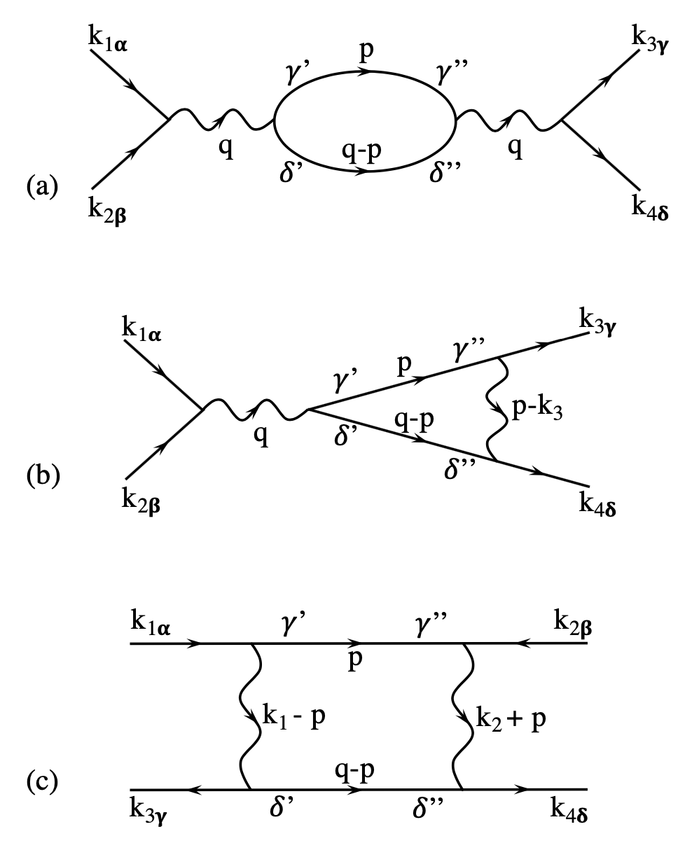
Figure 2: Feynman diagrams for one-loop corrections to the quartic vertex $R_{\alpha\beta,\gamma\delta}({\bf q})$, with (a) ”vacuum polarization” $\delta R^{(1)}_{\alpha\beta,\gamma\delta}({\bf q})$, (b) ”vertex correction” $\delta R^{(2)}_{\alpha\beta,\gamma\delta}({\bf q},{\bf k}_{3})$, (c) ”box diagram” $\delta R^{(3)}_{\alpha\beta,\gamma\delta}({\bf q},{\bf k}_{1})$.

To evaluate these integrals we now insert the decomposition $R_{\alpha\beta,\gamma\delta}(q)=\sum_{i=1}^{5}w_{i}(W_{i}(q))_{\alpha\beta,\gamma\delta}$ and use the definitions and the properties of the projectors summarized in Section A. We further use the formula for the angular averages (denoted $\langle\dots\rangle$, where $\hat{k}=k/|k|$) $\langle\hat{k}_{\alpha}\hat{k}_{\beta}\rangle=\frac{1}{D}\delta_{\alpha\beta}$ and $\langle\hat{k}_{\alpha}\hat{k}_{\beta}\hat{k}_{\gamma}\hat{k}_{\delta}\rangle=\frac{1}{D(D+2)}\left(\delta_{\alpha\beta}\delta_{\gamma\delta}+\delta_{\alpha\gamma}\delta_{\beta\delta}+\delta_{\alpha\delta}\delta_{\gamma\beta}\right)$LRReview .

Denoting $\delta w=(\delta w_{1},\delta w_{2},\delta w_{3},\delta w_{4},\delta w_{5})$ the one loop corrections to the couplings $w_{i}$ from the first diagram are

$$\delta w=\frac{-d_{c}}{D(D+2)}\bigg{(}2w_{1}^{2},2w_{2}^{2},(D+1)w_{3}^{2}+2\sqrt{D-1}w_{4}w_{3}+3w_{4}^{2},w_{4}(\sqrt{D-1}w_{4}+3w_{5})+w_{3}(Dw_{4}+\sqrt{D-1}w_{5}+w_{4}),$$

$$~{}~{}~{}~{}~{}~{}~{}~{}~{}~{}~{}~{}~{}~{}~{}~{}~{}~{}~{}~{}~{}~{}~{}~{}~{}~{}~{}~{}~{}~{}~{}~{}~{}~{}~{}~{}~{}~{}~{}(D+1)w_{4}^{2}+2\sqrt{D-1}w_{5}w_{4}+3w_{5}^{2}\bigg{)}\times\frac{T}{\kappa^{2}}{\int_{\Lambda_{\ell}e^{-d\ell}}^{\Lambda_{\ell}}{d^{D}p\over(2\pi)^{D}}}\frac{1}{p^{4}}$$ (110)

The contribution of the second diagram reads

$$\delta w=\frac{-4}{D(D+2)}\bigg{(}w_{1}(2w_{5}-w_{2}),w_{2}(2w_{5}-w_{2}),\frac{w_{2}}{2}((D^{2}-3)w_{3}+\sqrt{D-1}(D+1)w_{4})+w_{5}(Dw_{3}+\sqrt{D-1}w_{4}+w_{3}),$$ (111)

$$~{}~{}~{}\frac{w_{2}((D^{2}-1)w_{3}+\sqrt{D-1}(D^{2}+D-4)w_{4}+(D^{2}-1)w_{5})+2w_{5}((D-1)w_{3}+\sqrt{D-1}(D+4)w_{4}+(D-1)w_{5})}{4\sqrt{D-1}},$$

$$~{}~{}~{}~{}~{}~{}~{}~{}~{}~{}~{}~{}~{}w_{5}(\sqrt{D-1}w_{4}+3w_{5})+\frac{w_{2}}{2}(\sqrt{D-1}(D+1)w_{4}+(D-1)w_{5})\bigg{)}\times\frac{T}{\kappa^{2}}{\int_{\Lambda_{\ell}e^{-d\ell}}^{\Lambda_{\ell}}{d^{D}p\over(2\pi)^{D}}}\frac{1}{p^{4}}$$

The contribution of the third diagram reads

$$\delta w=\frac{-1}{D(D+2)}\bigg{(}\left(D^{2}-2\right)w_{2}^{2}+4Dw_{5}w_{2}+8w_{5}^{2},\left(D^{2}-2\right)w_{2}^{2}+4Dw_{5}w_{2}+8w_{5}^{2},$$

$$(D^{2}+D-3)w_{2}^{2}+4(D+1)w_{5}^{2}+4w_{5}w_{2},\sqrt{D-1}(w_{2}-2w_{5}){}^{2},(D^{2}-1)w_{2}^{2}+4(D-1)w_{5}w_{2}+12w_{5}^{2}\bigg{)}\frac{T}{\kappa^{2}}{\int_{\Lambda_{\ell}e^{-d\ell}}^{\Lambda_{\ell}}{d^{D}p\over(2\pi)^{D}}}\frac{1}{p^{4}}$$

where we have kept the explicit factors $D$ in the geometric factors.

.8 D 2. Correction to the bending rigidity $\kappa$

The correction to the self-energy to first order in perturbation theory $O(R)$ can be read off from (69) as

$$\delta\Sigma(k)=\frac{2T}{\kappa}k_{\alpha}k_{\delta}\int_{q}(k_{\beta}+q_{\beta})(k_{\gamma}+q_{\gamma})R_{\alpha\beta,\gamma\delta}({\bf q})\frac{1}{|{\bf k}+{\bf q}|^{4}}$$ (112)

from which we will identify the corrections to $\kappa$ and $\gamma$ from the small external momentum $k$ expansion

$$\delta\Sigma(k)=\delta\gamma\,k^{2}+\delta\kappa\,k^{4}+O(k^{6})$$ (113)

The calculation of (112) proceeds by inserting again $R_{\alpha\beta,\gamma\delta}({\bf q})=\sum_{i=1}^{5}w_{i}(W_{i}({\bf q}))_{\alpha\beta,\gamma\delta}$, performing the expansion at small $k$ of the numerator, and the resulting contractions of indices. In the course of the calculation one needs the leading behavior near $D=4$ and expansion in $k$ of three integrals. One uses the expansion

$$\frac{1}{|{\bf k}+{\bf q}|^{4}}=\frac{1}{q^{4}}(1-4\frac{{\bf k}\cdot{\bf q}}{q^{2}}-2\frac{k^{2}}{q^{2}}+12\frac{({\bf q}\cdot{\bf k})^{2}}{q^{4}}+O(k^{3}))$$ (114)

The first integral is

$$\int\frac{d^{D}q}{(2\pi)^{D}}\frac{1}{|{\bf q}+{\bf k}|^{4}}q_{\alpha}=\int\frac{d^{D}q}{(2\pi)^{D}}\frac{q_{\alpha}}{q^{4}}\left(1-4\frac{{\bf k}\cdot{\bf q}}{q^{2}}+O(k^{2})\right)=-4k_{\beta}\frac{\delta_{\alpha\beta}}{D}\int\frac{d^{D}q}{(2\pi)^{D}}\frac{1}{q^{4}}+O(k^{2})$$ (115)

It can also be obtained by taking the ratio $\lim_{b\to 0,D\to 4}\frac{I_{\alpha}(a=2,b)}{I(a=2,b)}=-p_{\alpha}$ using Eqs. A34 and A43 in LRReview .

The second integral is

$$\int\frac{d^{D}q}{|{\bf q}+{\bf k}|^{4}}\frac{q_{\alpha}q_{\beta}q_{\gamma}}{q^{2}}=\int\frac{d^{D}q}{q^{4}}\frac{q_{\alpha}q_{\beta}q_{\gamma}}{q^{2}}\left(1-4\frac{{\bf k}\cdot{\bf q}}{q^{2}}+O(k^{2})\right)$$ (116)

$$=-\frac{4}{D(D+2)}(\delta_{\alpha\beta}k_{\gamma}+\delta_{\alpha\gamma}k_{\beta}+k_{\alpha}\delta_{\beta\gamma})\int\frac{d^{D}q}{(2\pi)^{D}}\frac{1}{q^{4}}+O(k^{2})$$ (117)

One can check that this is also the result from A34 and A51 in LRReview , i.e. $\lim_{b\to 0,D\to 4,D=2a+2b}\frac{I_{\alpha\beta\gamma}(a=2,b+1)}{I(a=2,b)}$, being careful to obey the constraint $D=2a+2b$ when taking the limits.

The third integral is

$$\int\frac{d^{D}q}{|{\bf q}+{\bf k}|^{4}}q_{\alpha}q_{\beta}=\int\frac{d^{D}q}{q^{4}}q_{\alpha}q_{\beta}\left(1-4\frac{{\bf k}\cdot{\bf q}}{q^{2}}-2\frac{k^{2}}{q^{2}}+12\frac{({\bf q}\cdot{\bf k})^{2}}{q^{4}}\right)$$ (118)

$$=\frac{\delta_{\alpha\beta}}{D}\int\frac{d^{D}q}{(2\pi)^{D}}\frac{1}{q^{2}}-2k^{2}\frac{1}{D}\delta_{\alpha\beta}\int\frac{d^{D}q}{(2\pi)^{D}}\frac{1}{q^{4}}+\frac{12}{D(D+2)}k_{\gamma}k_{\delta}(\delta_{\alpha\beta}\delta_{\gamma\delta}+\delta_{\alpha\gamma}\delta_{\beta\delta}+\delta_{\alpha\delta}\delta_{\beta\gamma})\int\frac{d^{D}q}{(2\pi)^{D}}\frac{1}{q^{4}}$$ (119)

$$=\frac{\delta_{\alpha\beta}}{D}\int\frac{d^{D}q}{(2\pi)^{D}}\frac{1}{q^{2}}+\left(\frac{1}{D}\delta_{\alpha\beta}(-2+\frac{12}{D+2})k^{2}+\frac{24}{D(D+2)}k_{\alpha}k_{\beta}\right)\int\frac{d^{D}q}{(2\pi)^{D}}\frac{1}{q^{4}}$$ (120)

It can also be obtained from $\lim_{b\to 0,D\to 4}\frac{I_{\alpha\beta}(a=2,b)}{I(a=2,b)}=p_{\alpha}p_{\beta}$ from A34 and A48 in LRReview .

We finally obtain the corrections $\delta\gamma$ and $\delta\kappa$ as

$$\delta\gamma=\frac{2T}{\kappa}\frac{\left((D-1)w_{2}+2w_{5}\right)}{2D}\int\frac{d^{D}q}{(2\pi)^{D}}\frac{1}{q^{2}}=|_{D\to 4}\frac{2T}{\kappa}\frac{1}{8}\left(3w_{2}+2w_{5}\right)\int\frac{d^{D}q}{(2\pi)^{D}}\frac{1}{q^{2}}$$ (121)

$$\delta\kappa=\frac{2T}{\kappa}\frac{-\left(D^{2}+D-2\right)w_{2}+(D-2)(D+1)w_{1}+Dw_{3}-6\sqrt{D-1}w_{4}-2Dw_{5}+w_{3}+11w_{5}}{D(D+2)}\int\frac{d^{D}q}{(2\pi)^{D}}\frac{1}{q^{4}}$$ (122)

$$=|_{D\to 4}\frac{2T}{\kappa}\frac{1}{24}\left(10w_{1}-18w_{2}+5w_{3}-6\sqrt{3}w_{4}+3w_{5}\right)\int\frac{d^{D}q}{(2\pi)^{D}}\frac{1}{q^{4}}$$ (123)

where we will calculate the remaining integral using momentum shell $\int\frac{d^{D}q}{(2\pi)^{D}}\frac{1}{q^{4}}\to{\int_{\Lambda_{\ell}e^{-d\ell}}^{\Lambda_{\ell}}{d^{D}q\over(2\pi)^{D}}}\frac{1}{q^{4}}$. The correction $\delta\gamma$ (given by a UV divergent integral) obtained above is analogous to the usual non universal shift in the critical temperature for $O(N)$ models, and of little interest to us since we will tune the bare $\gamma$ so that the system is at its critical point $\gamma_{R}=0$ (i.e. $\gamma+\delta\gamma=0$). Said otherwise, the bare term in the model is $\frac{1}{2}(\gamma-\gamma_{c})(\nabla h)^{2}$.

.9 D 3. Final RG equations

We now use that the integral ${\int_{\Lambda_{\ell}e^{-d\ell}}^{\Lambda_{\ell}}{d^{D}p\over(2\pi)^{D}}}\frac{1}{p^{4}}=C_{D}\frac{1}{\epsilon}(e^{\epsilon d\ell}-1)\Lambda_{\ell}^{-\epsilon}=C_{4}\Lambda_{\ell}^{-\epsilon}d\ell+O(\epsilon)$ with $\epsilon=4-D$ and $C_{4}=\frac{1}{8\pi^{2}}$. We define the scaled dimensionless coupling

$$\tilde{w}_{i}=\frac{T}{\kappa^{2}}w_{i}C_{4}\Lambda_{\ell}^{-\epsilon}$$ (124)

To derive the flow equation we calculate $\partial_{\ell}\tilde{w}_{i}$ taking into account (i) the rescaling (ii) the sum of the three diagrams which correct $R$ (specifying $D=4$) leading to $\delta\tilde{w}_{i}=\beta_{i}[\tilde{w}]d\ell=\sum_{j,k}c_{ijk}\tilde{w}_{j}\tilde{w}_{k}d\ell$ (iii) the extra term from the correction $\delta(\kappa^{-2})=-\frac{2}{\kappa^{3}}\delta\kappa$ which leads to the $\eta$ function, $\eta[\tilde{w}]$. This leads to the RG equation

$$\partial_{\ell}\tilde{w}_{i}=\epsilon\tilde{w}_{i}+\beta_{i}[\tilde{w}]-2\eta[\tilde{w}]\tilde{w}_{i}\quad,\quad\eta[\tilde{w}]=\frac{\partial_{\ell}\kappa}{\kappa}$$ (125)

where (123) leads to (from now on for notational convenience we will suppress the tilde on $w$)

$$\eta[w]=\frac{1}{12}\left(10w_{1}-18w_{2}+5w_{3}+3w_{5}-6w_{44}\right)$$ (126)

gives the $\eta$ exponent at the fixed point. Putting all together, the final RG equations are (with $w_{44}=\sqrt{3}w_{4}$)

$$\partial_{\ell}w_{1}=\epsilon w_{1}+\frac{1}{12}\left(-(d_{c}+20)w_{1}^{2}+2\left(19w_{2}-5w_{3}-5w_{5}+6w_{44}\right)w_{1}-7w_{2}^{2}-4w_{5}^{2}-8w_{2}w_{5}\right)$$ (127)

$$\partial_{\ell}w_{2}=\epsilon w_{2}+\frac{1}{12}\left(-(d_{c}-31)w_{2}^{2}-20w_{1}w_{2}-2\left(5w_{3}+9w_{5}-6w_{44}\right)w_{2}-4w_{5}^{2}\right)$$

$$\partial_{\ell}w_{3}=\epsilon w_{3}+\frac{1}{24}\bigg{(}-5d_{c}w_{3}^{2}-d_{c}w_{44}^{2}-2d_{c}w_{3}w_{44}-17w_{2}^{2}+46w_{3}w_{2}$$

$$-10w_{44}w_{2}-20w_{3}^{2}-20w_{5}^{2}-40w_{1}w_{3}+24w_{3}w_{44}-4w_{5}\left(w_{2}+8w_{3}+w_{44}\right)\bigg{)}$$

$$\partial_{\ell}w_{44}=\epsilon w_{44}+\frac{1}{24}\bigg{(}-w_{44}\left(5(d_{c}+4)w_{3}+(d_{c}-24)w_{44}+40w_{1}\right)-w_{5}\left(3(d_{c}+2)w_{3}+(3d_{c}+28)w_{44}\right)$$

$$-3w_{2}^{2}+\left(-15w_{3}-3w_{5}+56w_{44}\right)w_{2}-18w_{5}^{2}\bigg{)}$$

$$\partial_{\ell}w_{5}=\epsilon w_{5}+\frac{1}{72}\left(-9(d_{c}+12)w_{5}^{2}-6w_{5}\left((d_{c}-10)w_{44}+20w_{1}-27w_{2}+10w_{3}\right)-5\left(d_{c}w_{44}^{2}+9w_{2}^{2}+6w_{44}w_{2}\right)\right)$$

Large $d_{c}$ limit. In the above RG equations (127) the couplings $w_{i}$ have not been rescaled by $1/d_{c}$. If one rescales them, and then take the large $d_{c}$ limit one obtains

$$\partial_{\ell}w_{1}=\epsilon w_{1}-\frac{w_{1}^{2}}{12}\ ,\quad\partial_{\ell}w_{2}=\epsilon w_{2}-\frac{w_{2}^{2}}{12}\ ,\quad\partial_{\ell}w_{3}=\epsilon w_{3}-\frac{1}{24}\left(5w_{3}^{2}+2w_{44}w_{3}+w_{44}^{2}\right)\ ,$$ (128)

$$\partial_{\ell}w_{44}=\epsilon w_{44}-\frac{1}{24}\left(3w_{5}\left(w_{3}+w_{44}\right)+w_{44}\left(5w_{3}+w_{44}\right)\right)\ ,\quad\partial_{\ell}w_{5}=\epsilon w_{5}-\frac{1}{72}\left(9w_{5}^{2}+6w_{44}w_{5}+5w_{44}^{2}\right).$$

Recall that $w_{i}$ here is in fact the rescaled coupling $\tilde{w}_{i}$ given in (124). Hence comparing with (92) (the factor $T$ being omitted there) we see that we can identify $w_{i}\equiv\frac{1}{8\pi^{2}}\hat{w}_{i}$. Inserting into (128) we obtain a set of RG equations for the $\hat{w}_{i}$ which, as one can check using $\lim_{\epsilon=4-D\to 0}\epsilon a_{i}(D,0)=\frac{1}{192\pi^{2}}\{2,2,5,\sqrt{3},3\}$ and $w_{44}=\sqrt{D-1}w_{4}$, agree exactly with the RG equations at large $d_{c}$ (93) for $D=4$. Finally note that $\eta[w]=O(1/d_{c})$ at large $d_{c}$ consistent with the SCSA and large $d_{c}$ expansion.

.10 D 4. Analysis of the RG equations

Instability of the isotropic membrane fixed point. The case of the rotationally invariant membrane is obtained setting $w_{2}=w_{4}=w_{5}=0$, which is a manifold preserved by the RG. The RG flow (127) then reduces within this subspace $(w_{1},w_{3})$ to

$$\partial_{\ell}w_{1}=\epsilon w_{1}-\frac{1}{12}w_{1}\left((d_{c}+20)w_{1}+10w_{3}\right)\ ,$$ (129)

$$\partial_{\ell}w_{3}=\epsilon w_{3}-\frac{5}{24}w_{3}\left((d_{c}+4)w_{3}+8w_{1}\right).$$ (130)

We recall that in that subspace $(w_{1},w_{3})$ are related to $(\mu,\lambda)$ via $w_{1}=\mu$ and $w_{3}=\mu+(D-1)\frac{\mu\lambda}{\lambda+2\mu}$ as obtained from (45), and given in (8) in the text. Using that relation one can derive RG equations for $\mu$ and $\lambda$ which can be checked to be identical to the one in Ref. AL (taking into account a difference by a factor of $4$ in the definition of $\mu,\lambda$ there). There are four fixed points

$$\left\{w_{1}\to 0,w_{3}\to\frac{24\epsilon}{5(d_{c}+4)}\right\},\left\{w_{1}\to\frac{12\epsilon}{d_{c}+24},w_{3}\to\frac{24\epsilon}{5(d_{c}+24)}\right\},\left\{w_{1}\to 0,w_{3}\to 0\right\},\left\{w_{1}\to\frac{12\epsilon}{d_{c}+20},w_{3}\to 0\right\}\ ,$$ (131)

which correspond to (in the same order footnote3 )

$$(\mu,\lambda)=(0,0);(\frac{12\epsilon}{24+d_{c}},\frac{-4\epsilon}{24+d_{c}});(0,\frac{2\epsilon}{d_{c}});(\frac{12\epsilon}{20+d_{c}},\frac{-6\epsilon}{20+d_{c}})\ .$$ (132)

The second one is the standard fixed point which describes the isotropic flat membrane within the $\epsilon$-expansion AL . The third one describes the fixed connectivity fluid (zero shear modulus), that is a model for nematic elastomer membranesLRelastomer . The fourth one is located on the line where the bulk modulus vanishes, i.e. $2\mu+D\lambda=\frac{2(D-1)w_{1}w_{3}}{Dw_{1}-w_{3}}=0$ which separates the thermodynamically stable and unstable regions of parameters, and controls the transition between these regions. The exponent $\eta$ is given by

$$\eta=\eta[w]=\frac{5}{12}(2w_{1}+w_{3})=\frac{5\mu(\lambda+\mu)}{2(\lambda+2\mu)}$$ (133)

and gives $\eta^{\rm iso}=\frac{12\epsilon}{24+d_{c}}$ for the isotropic membrane, as in AL .

Let us now discuss the stability of the isotropic membrane to the non-rotationally invariant terms (due to an external orienting field $\vec{E}$) in the model. For this we calculate the eigenvalues and associated eigenvectors (represented as columns) of the Hessian around the isotropic fixed point, which are given by

$$\left\{0,-\frac{\epsilon d_{c}}{d_{c}+24},\frac{\epsilon d_{c}}{d_{c}+24},\frac{\epsilon d_{c}}{d_{c}+24},-\epsilon\right\}$$ (134)

$$\left(\begin{array}[]{ccccc}\frac{16}{d_{c}+24}&-\frac{1}{2}&-\frac{19d_{c}+78}{5(d_{c}+12)}&-\frac{19d_{c}-6}{3(d_{c}+12)}&\frac{5}{2}\\ 0&0&\frac{1}{5}(-d_{c}-2)&-\frac{d_{c}}{3}&0\\ -\frac{2(d_{c}+8)}{5(d_{c}+24)}&1&-\frac{23d_{c}-24}{25(d_{c}+12)}&-\frac{26(d_{c}-6)}{15(d_{c}+12)}&1\\ 1&0&0&1&0\\ 0&0&1&0&0\\ \end{array}\right)\ .$$ (140)

The second and last columns are the two stable directions which are also obtained if one diagonalises the flow inside the isotropic subspace. In the full space of five couplings however, we see that the isotropic fixed point is unstable in two directions, with eigenvalue $\rho=\frac{\epsilon d_{c}}{d_{c}+24}$, and marginal in a third direction.

Crossover for small anisotropy. To discuss the effect of a small anisotropy let us first recall the analysis of the length scales in the isotropic membrane. The dimensionless couplings $\tilde{w}_{1},\tilde{w}_{3}$ (we temporarily restore the tilde) at scale $L$ are of order

$$\tilde{w}_{1,3}\sim\frac{TK_{0}}{\kappa^{2}}L^{4-D}\quad,\quad L<L_{\rm anh}\sim(\frac{\kappa^{2}}{TK_{0}})^{1/(4-D)}\ ,$$ (141)

$$\tilde{w}_{1,3}\simeq\tilde{w}^{*}_{1,3}\sim\frac{TK_{0}(L)}{\kappa(L)^{2}}L^{4-D}\quad,\quad L>L_{\rm anh}\ ,$$ (142)

where $L_{\rm anh}$ is the length scale below which the harmonic theory holds (and the elastic moduli and bending rigidity equal their bare values). For $L>L_{\rm anh}$ these are corrected and one has $\kappa(L)\sim\kappa(L/L_{\rm anh})^{\eta}$ and $K_{0}(L)\sim K_{0}(L/L_{\rm anh})^{-(4-D-2\eta)}$. The length $L_{\rm anh}$ is itself determined when $\tilde{w}_{1,3}$ reach numbers of order unity, of order their value at the fixed point.

Consider now the model in presence of very small bare symmetry breaking couplings $\mu_{1},\mu_{2},\lambda_{1},\lambda_{2}$ assumed to be of the same order. Then, from (45) the bare $w^{0}_{2},w^{0}_{5},w^{0}_{44}$ are linear combinations of those, hence small and of the same order. These couplings are relevant and grow as

$$\tilde{w}_{i}\sim\frac{Tw_{i}^{0}}{\kappa^{2}}L^{4-D}\quad,\quad L<L_{\rm anh}\ ,$$ (143)

$$\tilde{w}_{i}\sim\frac{Tw_{i}^{0}}{\kappa^{2}}L_{\rm anh}^{4-D}(\frac{L}{L_{\rm anh}})^{\rho}\quad,\quad L>L_{\rm anh}\ ,$$ (144)

where $w_{i}^{0}$ denote any linear combination of the bare symmetry breaking couplings ($i=2,4,5$) and $\rho$ was calculated above in the $\epsilon$ expansion. The length scale $L_{\rm anis}$ beyond which anisotropy will change the property of the system is obtained when $\tilde{w}_{i}$ becomes of order unity, hence

$$L_{\rm anis}\sim L_{\rm anh}(\frac{K_{0}}{w_{i}^{0}})^{1/\rho}\quad,\quad\rho=\frac{\epsilon d_{c}}{d_{c}+24}+O(\epsilon^{2})\ ,$$ (145)

whenever $w_{i}^{0}\sim\mu_{1,2},\lambda_{1,2}\ll K_{0}$.

Search for new fixed points

We now study the RG flow (127) in the five parameter space, for general codimension $d_{c}$.

For the physical case, $d_{c}=1$, we find 12 real fixed points. However all of them are repulsive, one with two unstable directions, the others with even more. Hence around $D=4$ there is no perturbative fixed point and we have a runaway RG flow.

We find that an attractive fixed point exists only for high enough $d_{c}$. The situation is very similar to the one for the crumpling transition, with $d$ replaced by $d_{c}$. For instance, for $d_{c}=220$ we find one, and only one, fully attractive fixed point

$$w_{i}=\{0.05063,0.05063,0.01912,\ -0.03150,0.04012\},$$ (146)

with eigenvalues ${-1.,-0.86129,-0.86129,-0.46296,-0.08355}$ One can check that this fixed point lies in the manifold

$$w_{1}=w_{2}=\mu_{0}\quad,\quad w_{3}=\frac{1}{2}(D-1)\lambda_{0}+\mu_{0}\quad,\quad w_{4}=\frac{1}{2}\sqrt{D-1}\lambda_{0}\quad,\quad w_{5}=\frac{1}{2}\lambda_{0}+\mu_{0}\ ,$$ (147)

with $\mu_{0}=0.050628$ and $\lambda_{0}=-0.021002$ This is the manifold mentioned in the text which leads to a purely local interaction between the tangent fields, i.e.

$$R_{\alpha\beta,\gamma\delta}(q)=\frac{\mu_{0}}{2}(\delta_{\alpha\gamma}\delta_{\beta\delta}+\delta_{\alpha\delta}\delta_{\beta\gamma})+\frac{\lambda_{0}}{2}\delta_{\alpha\beta}\delta_{\gamma\delta}\ .$$ (148)

One can check by inserting (147) into (127) that this manifold is preserved by the RG. Furthermore, inside this manifold one can check inserting (147) into (126) that $\eta[w]=0$ to the order $O(\epsilon)$, and that the RG flow can be written as

$$\partial_{\ell}\mu_{0}=\epsilon\mu_{0}+\frac{1}{12}\left(-(d_{c}+21)\mu_{0}^{2}-\lambda_{0}^{2}-10\lambda_{0}\mu_{0}\right)\ ,$$ (149)

$$\partial_{\ell}\lambda_{0}=\epsilon\lambda_{0}+\frac{1}{12}\left(-(6d_{c}+7)\lambda_{0}^{2}-2(3d_{c}+17)\lambda_{0}\mu_{0}-(d_{c}+15)\mu_{0}^{2}\right)\ .$$ (150)

Defining $u=\mu$ and $v=\lambda/2+\mu/4$ one can check that these equations are identical to the Eqs. (5a,b) in Ref. PKN (for their $u,v$) setting there $K_{4}=1/4$. Hence they are identical to those of the crumpling transition but with $d\to d_{c}$. From PKN we know that this fixed point exists only for $d>219$. This fixed point, which we interpret here as describing the anisotropic membrane in its flat phase at the buckling transition found here within the RG in the $D=4-\epsilon$ expansion is the one found within the SCSA (and large $d_{c}$) expansion described in the Section D4. While in the RG it disappears near $D=4$ for $d_{c}<219$, within the SCSA it survives for the physical dimension $D=2$ and $d_{c}=1$. Hence while the RG suggests a fluctuation driven first order transition in the physical dimension, the SCSA suggests a continuous transition. The question of which is the most accurate description is beyond the scope of the present work and would presumably require numerical simulations, as was the case for the crumpling transition (see e.g. MouhannaCrumpling for discussion and references).

E. Renormalization group for the $u,h$ theory

Here we perform the one loop RG study on the $u,h$ theory given in (35), (36), i.e. before integration over the phonons. It allows to obtain some extra information (the renormalization of $\mu$) and provides a useful check on the RG flow of the previous Section. We can rewrite the model as

$${\cal F}[u,\vec{h}]=\int d^{D}x\,\,\frac{1}{2}(\nabla^{2}h)^{2}+\frac{1}{2}(G^{u})^{-1}_{\alpha\beta}u_{\alpha}u_{\beta}+u_{\alpha}C^{\mu+\mu_{1},\lambda+\lambda_{1}}_{\alpha,\gamma\delta}A_{\gamma\delta}+\frac{1}{2}C^{\mu+\mu_{2},\lambda+\lambda_{2}}_{\alpha\beta,\gamma\delta}A_{\alpha\beta}A_{\gamma\delta}\quad,\quad C^{\mu,\lambda}_{\alpha,\gamma\delta}=-\partial_{\beta}C^{\mu,\lambda}_{\alpha\beta,\gamma\delta}\ ,$$ (151)

where we have defined, in Fourier space, the $uhh$ vertex

$$C^{1}_{\alpha,\gamma\delta}({\bf q})=C^{\mu+\mu_{1},\lambda+\lambda_{1}}_{\alpha,\gamma\delta}({\bf q})=-i\left((\lambda+\lambda_{1})q_{\alpha}\delta_{\gamma\delta}+(\mu+\mu_{1})(\delta_{\alpha\delta}q_{\gamma}+\delta_{\alpha\gamma}q_{\delta})\right)\ ,$$ (152)

and the bare phonon propagator

$$(G^{u})^{-1}_{\alpha\beta}({\bf q})=\mu P_{\alpha\beta}^{T}({\bf q})+(\lambda+2\mu)P_{\alpha\beta}^{L}({\bf q})\ .$$ (153)

Here we calculate the corrections to the vertices, hence we evaluate to lowest order in the perturbation theory in the nonlinearities, the vertices of the effective action $\Gamma_{uu},\Gamma_{uhh},\Gamma_{hhhh}$. These vertices will give us the corrections respectively to $(\mu,\lambda)$, $(\mu_{1},\lambda_{1})$ and $(\mu_{2},\lambda_{2})$. The corresponding diagrams are shown in the Fig.3.

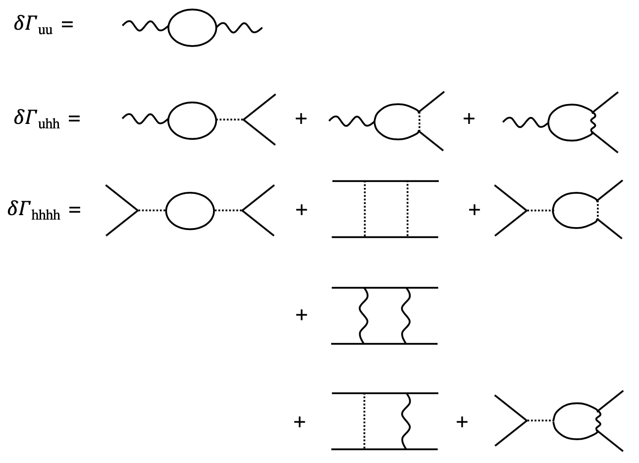
Figure 3: Feynman diagrams for one-loop corrections to the renormalized vertices in the $u-h$ description of the critical buckling membrane.

.11 E. 1 Calculation of $\Gamma_{uu}$

Let us calculate the one loop corrections to the phonon propagator, given by the single diagram in Fig.3. The effective action for the $u^{2}$ term is given, to one loop, as

$$\frac{1}{2}\int_{\bf q}u({\bf q})\cdot\Gamma_{uu}({\bf q})\cdot u(-{\bf q})=\int_{\bf q}\frac{1}{2}u_{\alpha}({\bf q})u_{\beta}(-{\bf q})[G^{-1}_{\alpha\beta}({\bf q})-C^{\mu+\mu_{1},\lambda+\lambda_{1}}_{\alpha,\gamma\delta}({\bf q})C^{\mu+\mu_{1},\lambda+\lambda_{1}}_{\alpha^{\prime},\gamma^{\prime}\delta^{\prime}}(-{\bf q})\langle A_{\gamma\delta}({\bf q})A_{\gamma^{\prime}\delta^{\prime}}(-{\bf q})\rangle_{0}]\ ,$$

where here and below $\cdot$ denotes index summations. We have the following average, performed with the quadratic action

$$\langle A_{\gamma\delta}({\bf q})A_{\gamma^{\prime}\delta^{\prime}}(-{\bf q})\rangle_{0}=\frac{1}{2}d_{c}\Pi_{\gamma\delta,\gamma^{\prime}\delta^{\prime}}({\bf q})\quad,\quad\Pi_{\alpha\beta,\gamma\delta}({\bf q})={\rm sym}\int_{p}p_{\alpha}(q_{\beta}-p_{\beta})p_{\delta}(q_{\gamma}-p_{\gamma})G({\bf p})G({\bf q}-{\bf p})\ ,$$ (155)

which leads to

$$(\Gamma_{uu})_{\alpha\beta}({\bf q})=G^{-1}_{\alpha\beta}({\bf q})-\frac{d_{c}}{2}C^{\mu+\mu_{1},\lambda+\lambda_{1}}_{\alpha,\gamma\delta}({\bf q})C^{\mu+\mu_{1},\lambda+\lambda_{1}}_{\alpha^{\prime},\gamma^{\prime}\delta^{\prime}}(-{\bf q})\Pi_{\gamma\delta,\gamma^{\prime}\delta^{\prime}}({\bf q})\ .$$ (156)

Within the Wilson RG and to leading order in $\epsilon$ one has

$$\Pi_{\alpha\beta,\gamma\delta}({\bf q})\simeq\frac{1}{\kappa^{2}}\int_{p}\frac{p_{\alpha}p_{\beta}p_{\delta}p_{\gamma}}{p^{8}}=\frac{1}{\kappa^{2}}S_{\alpha\beta,\gamma\delta}\int_{p}\frac{1}{p^{4}}\ ,$$ (157)

i.e., the dependence in the external momentum $q\ll p$ is subdominant, where $p$ is the internal momentum in the loop. We have defined

$$S^{(4)}_{\alpha\beta,\gamma\delta}=S_{\alpha\beta,\gamma\delta}=\frac{1}{D(D+2)}(\delta_{\alpha\beta}\delta_{\gamma\delta}+\delta_{\alpha\gamma}\delta_{\beta\delta}+\delta_{\alpha\delta}\delta_{\beta\gamma})\ .$$ (158)

Hence we obtain

$$\Gamma_{uu}(q)=G^{-1}(q)-\frac{d_{c}}{2\kappa^{2}}C^{1}({\bf q})\cdot S\cdot(C^{1}(-{\bf q}))^{T}\int_{p}\frac{1}{p^{4}}\ .$$ (159)

Replacing $\int_{p}\frac{1}{p^{4}}\to C_{4}\Lambda_{\ell}^{-\epsilon}$ and performing the contractions, one obtains the following corrections to $\mu$ and $\lambda$

$$\delta\mu=-\frac{d_{c}}{12\kappa^{2}}(\mu+\mu_{1})^{2}C_{4}\Lambda_{\ell}^{-\epsilon}d\ell\ ,$$ (160)

$$\delta\lambda=-\frac{d_{c}}{24\kappa^{2}}[12(\lambda+\lambda_{1})^{2}+2(\mu+\mu_{1})^{2}+12(\lambda+\lambda_{1})(\mu+\mu_{1})]C_{4}\Lambda_{\ell}^{-\epsilon}d\ell\ .$$

Exponent $\eta_{u}$. The first equation can be rewritten to obtain the anomalous dimension of the phonon field, i.e the exponent $\eta_{u}$ defined by $\mu(L)\sim L^{-\eta_{u}}$,

$$\eta_{u}=-\frac{\delta\mu}{\mu d\ell}=\frac{d_{c}}{12}g_{\mu}=\frac{d_{c}}{12}(\tilde{w}_{1}-\tilde{w}_{2})\ ,$$ (161)

where we have defined the proper dimensionless coupling $g_{\mu}=\frac{(\mu+\mu_{1})^{2}}{\mu\kappa^{2}}C_{4}\Lambda_{\ell}^{-\epsilon}$ which we related to the $\tilde{w}_{i}$ using (45) and (124). At the fixed point this gives the exponent $\eta_{u}$:

- at the isotropic membrane fixed point $\tilde{w}_{2}=0$ and $\tilde{w}_{1}=\frac{12\epsilon}{d_{c}+24}$, leading to $\eta_{u}=\frac{d_{c}\epsilon}{d_{c}+24}$. Since $\eta=\frac{12\epsilon}{d_{c}+24}$ we check, to first order in $\epsilon$ the exact relation (to all orders), $\eta_{u}=\epsilon-2\eta$ guaranteed by rotational invariance AL .

- at the anisotropic membrane fixed point $\tilde{w}_{1}=\tilde{w}_{2}$ hence $\eta_{u}=0$ to order $O(\epsilon)$. The relation $\eta_{u}=\epsilon-2\eta$ does not hold (since $\eta=0$ there, to $O(\epsilon)$).

Note that one can also define the screening exponent $\eta_{w}$ for the coupling constants $w_{i}$ such that $w_{i}(L)\sim L^{-\eta_{w}}$. It is given by the graphical corrections $\beta_{i}=\frac{\delta w_{i}}{w_{i}}$. Since the RG equation for the scaled dimensionless coupling $\tilde{w}_{i}$ reads $\partial_{\ell}\hat{w}_{i}=(\epsilon-2\eta(\hat{w})-\beta_{i}[\tilde{w}])\tilde{w}_{i}$, at any fixed point one must have $\beta_{i}=\epsilon-2\eta$. In presence of anisotropy, $\beta_{i}$ becomes different from $\eta_{u}$. The nonlinear interactions are still screened, since $\eta<\epsilon/2$ at the anisotropic fixed point, but this screening is not directly related to the renormalization of $\mu$ and $\lambda$.

.12 E 2. Calculation of $\Gamma_{uhh}$

We now calculate the vertex corrections given by the three diagrams in Fig.3. They are corrections to the term $uhh$ in (151), which we write in the form

$$\int_{q}u_{\alpha}(-{\bf q})\,\delta V_{\alpha,\beta\gamma}({\bf q})\,A_{\beta\gamma}({\bf q})\ .$$ (162)

One obtains for the first diagram

$$\delta V^{(1)}_{\alpha,\beta\gamma}({\bf q})=-\frac{d_{c}}{2}(C^{1}({\bf q})\cdot S\cdot C^{2})_{\alpha,\beta\gamma}\frac{1}{\kappa^{2}}\int_{\bf p}\frac{1}{p^{4}}\ ,$$ (163)

where $C^{1}({\bf q})$ is the three index tensor given in (152) (i.e., the bare $uhh$ vertex) and we denote here and below $C^{2}$ the four index tensor $C^{\mu+\mu_{2},\lambda+\lambda_{2}}_{\alpha\beta,\gamma\delta}$ (entering the bare $h^{4}$ vertex) defined in (35). The second diagram gives the correction

$$\delta V^{(2)}_{\alpha,\beta\gamma}({\bf q})=-C^{1}_{\alpha,\alpha^{\prime}\alpha^{\prime\prime}}({\bf q})S_{\alpha^{\prime}\beta^{\prime}\alpha^{\prime\prime}\gamma^{\prime}}C^{2}_{\beta^{\prime}\beta,\gamma^{\prime}\gamma}\frac{1}{\kappa^{2}}\int_{\bf p}\frac{1}{p^{4}}\ .$$ (164)

Finally, the third diagram gives, using that $C^{1}_{\beta,\gamma\delta}({\bf q})=-iq_{\alpha}C^{1}_{\alpha\beta,\gamma\delta}$ (where the momentum independent four index tensor $C^{\mu+\mu_{1},\lambda+\lambda_{1}}_{\alpha\beta,\gamma\delta}$ is denoted $C^{1}$)

$$\delta V^{(3)}_{\alpha,\beta\gamma}({\bf q})=C^{1}_{\alpha,\beta^{\prime}\gamma^{\prime}}({\bf q})\left[S^{(8)}_{\beta^{\prime}\gamma^{\prime}\beta^{\prime\prime}\gamma^{\prime\prime}s^{\prime}s^{\prime\prime}\alpha^{\prime}\alpha^{\prime\prime}}\left(\frac{1}{2\mu+\lambda}-\frac{1}{\mu}\right)+\frac{1}{\mu}S^{(6)}_{\beta^{\prime}\gamma^{\prime}\beta^{\prime\prime}\gamma^{\prime\prime}s^{\prime}s^{\prime\prime}}\delta_{\alpha^{\prime}\alpha^{\prime\prime}}\right]C^{1}_{\alpha^{\prime}s^{\prime},\beta^{\prime\prime}\beta}C^{1}_{\alpha^{\prime\prime}s^{\prime\prime},\gamma^{\prime\prime}\gamma}\frac{1}{\kappa^{2}}\int_{\bf p}\frac{1}{p^{4}},$$

where we defined the 6 and 8 index symmetric tensors, schematically,

$$S^{(6)}_{\beta^{\prime}\gamma^{\prime}\beta^{\prime\prime}\gamma^{\prime\prime}s^{\prime}s^{\prime\prime}}=\frac{1}{D(D+2)(D+4)}(\delta\delta\delta+14\ \text{terms})\ ,$$ (166)

$$S^{(8)}_{\beta^{\prime}\gamma^{\prime}\beta^{\prime\prime}\gamma^{\prime\prime}s^{\prime}s^{\prime\prime}\alpha^{\prime}\alpha^{\prime\prime}}=\frac{1}{D(2+D)(4+D)(6+D)}(\delta\delta\delta\delta+104\ \text{terms})\ .$$ (167)

Performing the contractions we obtain for $i=1,2,3$

$$\delta V^{(i)}_{\alpha,\beta\gamma}({\bf q})=[A_{i}q_{\alpha}\delta_{\beta\gamma}+B_{i}(q_{\beta}\delta_{\alpha\gamma}+q_{\gamma}\delta_{\alpha\beta})]\frac{1}{\kappa^{2}}\int_{\bf p}\frac{1}{p^{4}}\ .$$ (168)

To display the results more compactly we define the new variables

$$\Lambda_{i}=\lambda_{i}+\lambda\quad,\quad M_{i}=\mu_{i}+\mu\quad,\quad i=1,2\ .$$ (169)

In terms of these variables the coefficients $A_{i},B_{i}$ read

$$A_{1}=-\frac{d_{c}}{12}\left(3\Lambda_{1}\left(2\Lambda_{2}+M_{2}\right)+M_{1}\left(3\Lambda_{2}+M_{2}\right)\right)\quad,\quad B_{1}=-\frac{d_{c}}{12}M_{1}M_{2}\ ,$$ (170)

$$A_{2}=\frac{1}{12}\left(-3\Lambda_{1}\left(\Lambda_{2}+5M_{2}\right)-M_{1}\left(\Lambda_{2}+7M_{2}\right)\right)\quad,\quad B_{2}=-\frac{1}{12}M_{1}\left(\Lambda_{2}+M_{2}\right)\ ,$$

$$A_{3}=\frac{3\Lambda_{1}^{3}\mu+\Lambda_{1}M_{1}^{2}(9\lambda+34\mu)+M_{1}^{3}(5\lambda+14\mu)+13\Lambda_{1}^{2}\mu M_{1}}{12\mu(\lambda+2\mu)}\quad,\quad B_{3}=\frac{M_{1}\left(\Lambda_{1}^{2}\mu+M_{1}^{2}(-(\lambda-2\mu))+4\Lambda_{1}\mu M_{1}\right)}{12\mu(\lambda+2\mu)}\ .$$

From these coefficients we directly obtain the corrections

$$\delta\Lambda_{1}=(A_{1}+A_{2}+A_{3})\frac{1}{\kappa^{2}}\int_{\bf p}\frac{1}{p^{4}}\quad,\quad\delta M_{1}=(B_{1}+B_{2}+B_{3})\frac{1}{\kappa^{2}}\int_{\bf p}\frac{1}{p^{4}}\ .$$ (171)

Putting all contributions together and replacing $\int_{\bf p}\frac{1}{p^{4}}\to C_{4}\Lambda_{\ell}^{-\epsilon}$, we obtain, from the vertex corrections

$$\delta M_{1}=\frac{1}{12}M_{1}\left(M_{2}\left(-\left(d_{c}+1\right)\right)-\Lambda_{2}+\frac{\Lambda_{1}^{2}\mu+M_{1}^{2}(-(\lambda-2\mu))+4\Lambda_{1}\mu M_{1}}{\mu(\lambda+2\mu)}\right)\frac{1}{\kappa^{2}}C_{4}\Lambda_{\ell}^{-\epsilon}d\ell\ ,$$ (172)

$$\delta\Lambda_{1}=\frac{1}{12}\bigg{(}-d_{c}\left(3\Lambda_{1}\left(2\Lambda_{2}+M_{2}\right)+M_{1}\left(3\Lambda_{2}+M_{2}\right)\right)$$

$$+\frac{3\Lambda_{1}^{3}\mu+\Lambda_{1}M_{1}^{2}(9\lambda+34\mu)+M_{1}^{3}(5\lambda+14\mu)+13\Lambda_{1}^{2}\mu M_{1}}{\mu(\lambda+2\mu)}-3\Lambda_{1}\left(\Lambda_{2}+5M_{2}\right)-M_{1}\left(\Lambda_{2}+7M_{2}\right)\bigg{)}\frac{1}{\kappa^{2}}C_{4}\Lambda_{\ell}^{-\epsilon}d\ell\ .$$

To recover the result for the isotropic membrane one sets $\Lambda_{i}=\lambda$ and $M_{i}=\mu$ and the above corrections reduce to

$$\delta\mu=-\frac{d_{c}}{12\kappa^{2}}\mu^{2}C_{4}\Lambda_{\ell}^{-\epsilon}d\ell\ ,$$ (173)

$$\delta\lambda=-\frac{d_{c}}{12\kappa^{2}}\left(6\lambda^{2}+6\lambda\mu+\mu^{2}\right)C_{4}\Lambda_{\ell}^{-\epsilon}d\ell\ .$$

This simplification occurs because the second and third diagram exactly cancel due to rotational invariance. Indeed the corrections (173) coincide with (160) (setting $\mu_{1}=\lambda_{1}=0$ there).

.13 E. 3 Calculation of $\Gamma_{hhhh}$

We now calculate the corrections to the $h^{4}$ vertex in (151). They are given by the six diagrams in Fig.3. We recall that we denote $C^{2}$ the four index tensor $C^{\mu+\mu_{2},\lambda+\lambda_{2}}_{\alpha\beta,\gamma\delta}$ which appears in the bare $h^{4}$ vertex.

The first diagram gives the following correction to $C^{2}$

$$\delta C^{2}=-\frac{d_{c}}{2}C^{2}\cdot S\cdot C^{2}\frac{1}{\kappa^{2}}\int_{\bf p}\frac{1}{p^{4}}\ .$$ (174)

The second and third diagram give respectively

$$\delta C^{2}_{\alpha\beta,\gamma\delta}=-2{\rm sym}\,C^{2}_{\alpha\alpha^{\prime},\gamma\gamma^{\prime}}C^{2}_{\beta\beta^{\prime},\delta\delta^{\prime}}S_{\alpha^{\prime}\beta^{\prime}\gamma^{\prime}\delta^{\prime}}\frac{1}{\kappa^{2}}\int_{\bf p}\frac{1}{p^{4}}\quad,\quad\delta C^{2}_{\alpha\beta,\gamma\delta}=-2\,C^{2}_{\alpha\beta,\alpha^{\prime}\beta^{\prime}}S_{\alpha^{\prime}\beta^{\prime}\gamma^{\prime}\delta^{\prime}}C^{2}_{\gamma\gamma^{\prime},\delta\delta^{\prime}}\frac{1}{\kappa^{2}}\int_{\bf p}\frac{1}{p^{4}}\ .$$ (175)

The fourth diagram is more complicated

$$\delta C^{2}_{\alpha\beta,\gamma\delta}=-2C^{1}_{r_{1}s_{1},\alpha\alpha^{\prime}}C^{1}_{r_{2}s_{2},\gamma\gamma^{\prime}}C^{1}_{r_{3}s_{3},\beta\beta^{\prime}}C^{1}_{r_{4}s_{4},\delta\delta^{\prime}}\bigg{[}\langle\hat{p}_{\alpha^{\prime}}\hat{p}_{\beta^{\prime}}\hat{p}_{\gamma^{\prime}}\hat{p}_{\delta^{\prime}}\hat{p}_{s_{1}}\hat{p}_{s_{2}}\hat{p}_{s_{3}}\hat{p}_{s_{4}}\hat{p}_{r_{1}}\hat{p}_{r_{2}}\hat{p}_{r_{3}}\hat{p}_{r_{4}}\rangle\left(\frac{1}{\lambda+2\mu}-\frac{1}{\mu}\right)^{2}$$ (176)

$$+\left(\langle\hat{p}_{\alpha^{\prime}}\hat{p}_{\beta^{\prime}}\hat{p}_{\gamma^{\prime}}\hat{p}_{\delta^{\prime}}\hat{p}_{s_{1}}\hat{p}_{s_{2}}\hat{p}_{s_{3}}\hat{p}_{s_{4}}\hat{p}_{r_{3}}\hat{p}_{r_{4}}\rangle\delta_{r_{1}r_{2}}+\langle\hat{p}_{\alpha^{\prime}}\hat{p}_{\beta^{\prime}}\hat{p}_{\gamma^{\prime}}\hat{p}_{\delta^{\prime}}\hat{p}_{s_{1}}\hat{p}_{s_{2}}\hat{p}_{s_{3}}\hat{p}_{s_{4}}\hat{p}_{r_{1}}\hat{p}_{r_{2}}\rangle\delta_{r_{3}r_{4}}\right)\frac{1}{\mu}\left(\frac{1}{\lambda+2\mu}-\frac{1}{\mu}\right)$$

$$+\frac{1}{\mu^{2}}S^{(8)}_{\alpha^{\prime}\beta^{\prime}\gamma^{\prime}\delta^{\prime}s_{1}s_{2}s_{3}s_{4}}\delta_{r_{1}r_{2}}\delta_{r_{3}r_{4}}\bigg{]}\frac{1}{\kappa^{2}}\int_{\bf q}\frac{1}{q^{4}}\ ,$$

where $\langle\dots\rangle$ denote angular averages and $\hat{\bf p}={\bf p}/p$ a unit vector. It was convenient to use that notational trick, rather than the symmetric tensors of order 10 and 12, as it allows the contractions to be taken more easily. This is equal to

$$\delta C^{2}_{\alpha\beta,\gamma\delta}=\bigg{(}-2C^{1}_{r_{1}s_{1},\alpha\alpha^{\prime}}C^{1}_{r_{2}s_{2},\gamma\gamma^{\prime}}C^{1}_{r_{3}s_{3},\beta\beta^{\prime}}C^{1}_{r_{4}s_{4},\delta\delta^{\prime}}\frac{1}{\mu^{2}}S^{(8)}_{\alpha^{\prime}\beta^{\prime}\gamma^{\prime}\delta^{\prime}s_{1}s_{2}s_{3}s_{4}}\delta_{r_{1}r_{2}}\delta_{r_{3}r_{4}}$$ (177)

$$-2\left(\frac{1}{\lambda+2\mu}-\frac{1}{\mu}\right)^{2}(\Lambda_{1}+2M_{1})^{4}S_{\alpha\beta\gamma\delta}$$

$$-2\left(\frac{1}{\lambda+2\mu}-\frac{1}{\mu}\right)\frac{1}{\mu}(\Lambda_{1}+2M_{1})^{2}[2((\Lambda_{1}+2M_{1})^{2}-M_{1}^{2})S_{\alpha\beta\gamma\delta}+\frac{M_{1}^{2}}{D}(\delta_{\alpha\gamma}\delta_{\beta\delta}+\delta_{\alpha\delta}\delta_{\beta\gamma})]\bigg{)}\frac{1}{\kappa^{2}}\int_{\bf p}\frac{1}{p^{4}}\ .$$

The fifth diagram leads to the correction

$$\delta C^{2}_{\alpha\beta,\gamma\delta}={\rm sym}\,4C^{1}_{r_{1}s_{1},\alpha\alpha^{\prime}}C^{1}_{r_{2}s_{2},\gamma\gamma^{\prime}}C^{2}_{\beta^{\prime}\beta,\delta^{\prime}\delta}\bigg{[}\left(\frac{1}{\lambda+2\mu}-\frac{1}{\mu}\right)S^{(8)}_{\alpha^{\prime}\beta^{\prime}\gamma^{\prime}\delta^{\prime}s_{1}s_{2}r_{1}r_{2}}+\frac{1}{\mu}S_{\alpha^{\prime}\beta^{\prime}\gamma^{\prime}\delta^{\prime}s_{1}s_{2}}\delta_{r_{1}r_{2}}\bigg{]}\frac{1}{\kappa^{2}}\int_{\bf q}\frac{1}{q^{4}}\ ,$$ (178)

and finally, the sixth diagram, to

$$\delta C^{2}_{\alpha\beta,\gamma\delta}={\rm sym}\,2C^{2}_{\alpha\beta,\alpha^{\prime}\beta^{\prime}}C^{1}_{r_{1}s_{1},\delta\delta^{\prime}}C^{1}_{r_{2}s_{2},\gamma\gamma^{\prime}}\bigg{[}\left(\frac{1}{\lambda+2\mu}-\frac{1}{\mu}\right)S^{(8)}_{\alpha^{\prime}\beta^{\prime}\gamma^{\prime}\delta^{\prime}s_{1}s_{2}r_{1}r_{2}}+\frac{1}{\mu}S_{\alpha^{\prime}\beta^{\prime}\gamma^{\prime}\delta^{\prime}s_{1}s_{2}}\delta_{r_{1}r_{2}}\bigg{]}\frac{1}{\kappa^{2}}\int_{\bf q}\frac{1}{q^{4}}\ .$$ (179)

Performing the contractions, in total we find for the corrections to the $h^{4}$ vertex

$$\delta M_{2}=\frac{1}{12}\bigg{[}\frac{-1}{\mu^{2}(\lambda+2\mu)^{2}}\bigg{(}\mu^{2}M_{2}^{2}\left(d_{c}+21\right)(\lambda+2\mu)^{2}+\Lambda_{1}^{4}\mu^{2}+M_{1}^{4}\left(7\lambda^{2}+44\lambda\mu+76\mu^{2}\right)$$ (180)

$$+8\Lambda_{1}\mu M_{1}\left(2M_{1}^{2}(\lambda+4\mu)-5\mu M_{2}(\lambda+2\mu)\right)+2\Lambda_{1}^{2}\mu\left(2M_{1}^{2}(\lambda+8\mu)-5\mu M_{2}(\lambda+2\mu)\right)\frac{1}{\kappa^{2}}C_{4}\Lambda_{\ell}^{-\epsilon}$$

$$-20\mu M_{2}M_{1}^{2}(\lambda+2\mu)(\lambda+4\mu)+8\Lambda_{1}^{3}\mu^{2}M_{1}\bigg{)}-\Lambda_{2}^{2}+2\Lambda_{2}\left(\frac{\Lambda_{1}^{2}\mu+2M_{1}^{2}(\lambda+4\mu)+4\Lambda_{1}\mu M_{1}}{\mu(\lambda+2\mu)}-5M_{2}\right)\bigg{]}\frac{1}{\kappa^{2}}C_{4}\Lambda_{\ell}^{-\epsilon}d\ell\ ,$$

and

$$\delta\Lambda_{2}=\frac{1}{12}\bigg{[}]-\Lambda_{2}^{2}\left(6d_{c}+7\right)-2\Lambda_{2}M_{2}\left(3d_{c}+17\right)+M_{2}^{2}\left(-\left(d_{c}+15\right)\right)-\frac{\left(\Lambda_{1}^{2}\mu+M_{1}^{2}(-(\lambda-2\mu))+4\Lambda_{1}\mu M_{1}\right){}^{2}}{\mu^{2}(\lambda+2\mu)^{2}}$$

$$+\frac{4M_{2}\left(\Lambda_{1}^{2}\mu+2M_{1}^{2}(\lambda+4\mu)+4\Lambda_{1}\mu M_{1}\right)}{\mu(\lambda+2\mu)}+\frac{8\Lambda_{2}\left(\Lambda_{1}^{2}\mu+2M_{1}^{2}(\lambda+4\mu)+4\Lambda_{1}\mu M_{1}\right)}{\mu(\lambda+2\mu)}\bigg{]}\frac{1}{\kappa^{2}}C_{4}\Lambda_{\ell}^{-\epsilon}d\ell\ .$$ (181)

To recover the result for the isotropic membrane one sets $\Lambda_{i}=\lambda$ and $M_{i}=\mu$ and the above corrections reduce exactly, once again, to (173). Here the simplification arises from the last five diagram cancelling due to rotational invariance.

.14 E. 4 Final RG equations

We can now put together $\delta\mu$, $\delta\lambda$ from (160), $\delta M_{1}=\delta\mu+\delta\mu_{1}$, $\delta\Lambda_{1}=\delta\lambda+\delta\lambda_{1}$ from (172), and $\delta M_{2}=\delta\mu+\delta\mu_{2}$, $\delta\Lambda_{2}=\delta\lambda+\delta\lambda_{2}$ from (180). This leads to the complete set of corrections to the six couplings, which is bulky and which we will not display here in full (see below). Let us denote $m_{i}$, $i=1,\dots,6$ these couplings. These corrections read schematically $\delta m_{i}=d_{ijk}m_{j}m_{k}$. To obtain the final RG flow one defines scaled dimensionless couplings $\tilde{m}_{i}$, as in (124), and take into account the corrections to $\kappa$ as we did in (125), leading to $\partial_{\ell}\tilde{m}_{i}=\epsilon\tilde{m}_{i}+d_{ijk}\tilde{m}_{j}\tilde{m}_{k}-2\eta[w[m]]\tilde{m}_{i}$. Here we denote $w[m]$ the $w_{i}$ expressed as functions of the $m_{i}$ via the Eq. (45), and we have used the same formula (126) for the $\eta[w]$ function.

To check that these are consistent with the RG equations obtained via the quartic theory in Section D, we simply need to compare the above corrections $\delta m$ and $\delta w$, i.e summing (.7), (111) and (.7) which can be written as $\delta w_{i}=\beta_{i}[w]d\ell=c_{ijk}w_{j}w_{k}d\ell$. We have performed the check as follows. We have evaluated in two ways

$$\delta w_{i}[m]=\frac{\partial w_{i}[m]}{\partial m_{j}}\delta m_{j}=\frac{\partial w_{i}[m]}{\partial m_{j}}d_{ijk}m_{j}m_{k}d\ell\ ,$$ (182)

$$\delta w_{i}[m]=c_{ijk}w_{j}[m]w_{k}[m]d\ell\ ,$$ (183)

and using $w[m]$ from Eq. (45) we have shown using Mathematica that the two lines above are identical functions of the $m_{i}$. This provides a quite non trivial check of these two lengthy calculations. Hence the RG equation for the 5 couplings $w_{i}$ can be deduced from the one for the 6 couplings $m_{i}$. The reverse is not true however, there is, in the general case, additional information in the 6 coupling flow, as we discussed above in Section E. 1 it allows to obtain $\delta\mu$ and from it we obtained there the exponent $\eta_{u}$, related to the anomalous dimension of the phonon field. Let us indicate for completeness the combination of couplings which enters the exponent $\eta$

$$\eta=\frac{1}{12}\left(10w_{1}-18w_{2}+5w_{3}+3w_{5}-6w_{44}\right)=\frac{M_{1}\left(2\Lambda_{1}\mu+3\lambda M_{1}+5\mu M_{1}\right)}{2\mu(\lambda+2\mu)}\ .$$ (184)

To express the RG flow it is natural to define the dimensionless ratio $r=\lambda/\mu$ and the four dimensionless coupling constants associated to the nonlinear terms in the action

$$\tilde{M}_{1}^{2}=\frac{M_{1}^{2}}{\mu\kappa^{2}}C_{4}\Lambda_{\ell}^{-\epsilon}\quad,\quad\tilde{\Lambda}_{1}^{2}=\frac{\Lambda_{1}^{2}}{\mu\kappa^{2}}C_{4}\Lambda_{\ell}^{-\epsilon}\quad,\quad\tilde{M}_{2}=\frac{M_{2}}{\kappa^{2}}C_{4}\Lambda_{\ell}^{-\epsilon}\quad,\quad\tilde{\Lambda}_{2}=\frac{\Lambda_{2}}{\kappa^{2}}C_{4}\Lambda_{\ell}^{-\epsilon}\ ,$$ (185)

and then $\mu$ can still flow with eigenvalue $\eta_{u}$. Since the RG equations for these couplings are bulky let us only display them here to leading order in large $d_{c}$, and we have dropped the tilde for notational convenience

$$\partial_{\ell}r=\frac{1}{12}d_{c}\left(-6\Lambda_{1}^{2}+rM_{1}^{2}-6\Lambda_{1}M_{1}-M_{1}^{2}\right)\quad,\quad\partial_{\ell}M_{1}=\frac{\epsilon}{2}M_{1}+\frac{1}{24}M_{1}\left(M_{1}^{2}-2M_{2}\right)d_{c}\ ,$$ (186)

$$\partial_{\ell}\Lambda_{1}=\frac{\epsilon}{2}\Lambda_{1}+\frac{1}{24}d_{c}\left(-12\Lambda_{1}\Lambda_{2}+\Lambda_{1}M_{1}^{2}-6\Lambda_{2}M_{1}-6\Lambda_{1}M_{2}-2M_{2}M_{1}\right)\ ,$$ (187)

$$\partial_{\ell}M_{2}=\epsilon M_{2}-\frac{1}{12}M_{2}^{2}d_{c}\quad,\quad\partial_{\ell}\Lambda_{2}=\epsilon\Lambda_{2}+\frac{1}{12}d_{c}\left(-6\Lambda_{2}^{2}-6\Lambda_{2}M_{2}-M_{2}^{2}\right)\ .$$ (188)

It is easy to see that the only attractive fixed point of these equations (and of the complete equations for any $d_{c}>219$) is such that

$$M_{1}=0\quad,\quad\Lambda_{1}=0\quad,\quad M_{2}=\frac{12}{d_{c}}+O(\frac{1}{d_{c}^{2}})\quad,\quad\Lambda_{2}=-\frac{4}{d_{c}}+O(\frac{1}{d_{c}^{2}})\ .$$ (189)

This is in agreement with the RG analysis using the $h^{4}$ theory presented above. Indeed this anisotropic fixed point lies in the manifold (147) in the $w_{i}$ variables, which in the current variables imply the constraints $\mu+\mu_{1}=0$, $\mu_{0}=\mu+\mu_{2}$, $\lambda_{0}=\lambda+\lambda_{2}-\frac{(\lambda+\lambda_{1})^{2}}{\lambda+2\mu}$. The fixed point (189) obeys these constraints and one can check that the values for $M_{2}$ and $\Lambda_{2}$ are consistent with those for the fixed point of (149) at large $d_{c}$ (and in fact, as one can check, for any $d_{c}>219$).

Since the couplings $M_{1}$ and $\Lambda_{1}$ flow to zero exponentially with $\ell$, at the anisotropic fixed point we see that the flow of $r=\lambda/\mu$ and the flow of $\mu$, which is given (exactly) by

$$\frac{1}{\mu}\partial_{\ell}\mu=-\frac{1}{12}M_{1}^{2}d_{c}-\frac{M_{1}\left(2\Lambda_{1}+(3r+5)M_{1}\right)}{r+2}$$ (190)

lead to finite, but non-universal values for $\lambda$ and $\mu$. This is consistent with the exponent $\eta_{u}=0$ as claimed above.

F. Renormalization group flow of $\gamma$

Until now we have assumed $\gamma$ (and $\tau$) to be tuned so that the system is at the critical point (the buckling transition), i.e. $\gamma_{R}=0$. Now we assume a small deviations away and calculate the RG flow of $\gamma$, and the associated (independent) critical exponent $\nu$. To check consistency, we perform the calculation both in the $h^{4}$ theory and in the $uh^{2}+h^{4}$ theory.

.15 F.1. Flow of $\gamma$ in quartic $h^{4}$ theory

To obtain the flow of $\gamma$ to linear order in $\gamma$, we expand the height field propagator at small $\gamma$ as

$$G(k)=\frac{1}{\kappa k^{4}+\gamma k^{2}}=\frac{1}{\kappa k^{4}}-\frac{\gamma}{\kappa^{2}k^{6}}+O(\gamma^{2})\ .$$ (191)

Let us call here $\delta\Sigma(k)=\delta\gamma k^{2}+O(k^{4})$ the part of the self-energy proportional to $O(\gamma)$ at small $\gamma$ (there is also a $O(1)$ part calculated in Section D.2 which determines the shift in the critical point $\gamma_{c}$ (see discussion there) but which is of no interest to us here. To lowest order in perturbation theory the self-energy is given by two diagrams, the sunset diagram in (112), leading to $\delta\gamma^{s}$, and the tadpole diagram $\delta\gamma^{t}$, with $\delta\gamma=\delta\gamma^{s}+\delta\gamma^{t}$. From the sunset diagram one has from (112)

$$\delta\Sigma^{s}({\bf k})=-\frac{\gamma}{\kappa^{2}}k_{\alpha}k_{\gamma}{2\over d_{c}}\sum_{i=1,5}w_{i}\int_{q}\frac{1}{(k-q)^{6}}(k_{\beta}-q_{\beta})(W_{i})_{\alpha\beta,\gamma\delta}({\bf q})(k_{\delta}-q_{\delta})=\delta\gamma^{s}\,k^{2}+O(k^{4})\ .$$ (192)

Within Wilson RG, to lowest order in $\epsilon$ one can write

$$\delta\Sigma^{s}({\bf k})=-\frac{\gamma}{\kappa^{2}}k_{\alpha}k_{\gamma}{2\over d_{c}}\sum_{i=1,5}w_{i}\int_{\bf q}\frac{q_{\beta}q_{\delta}}{q^{6}}(W_{i})_{\alpha\beta,\gamma\delta}({\bf q})=-\frac{\gamma}{\kappa^{2}}k^{2}{2\over d_{c}}\left[\left(\frac{1}{2}-\frac{1}{2D}\right)w_{2}+\frac{1}{D}w_{5}\right]\int_{\bf q}\frac{1}{q^{4}}\ .$$ (193)

In addition there is the tadpole contribution, leading to the $O(\gamma)$ correction $\delta\gamma^{t}$

$$\Sigma^{\rm t}(k)=k_{\alpha}k_{\gamma}R^{0}_{\alpha\beta,\gamma\delta}\int_{q}q_{\gamma}q_{\delta}G(q)\quad\Rightarrow\quad\delta\gamma^{t}k^{2}=-\gamma k_{\alpha}k_{\gamma}R^{0}_{\alpha\beta,\gamma\delta}\langle q_{\gamma}q_{\delta}\rangle\frac{1}{\kappa^{2}}\int_{\bf q}\frac{1}{q^{4}}\ ,$$ (194)

where $R^{0}$ is the ${\bf k}=0$ component of the vertex. From (59) it is equal to $R^{0}=\frac{1}{2}\bar{C}$ where $\bar{C}$ given in (60), and more explicitly, from (61)

$$R^{0}_{\alpha\beta,\gamma\delta}=\frac{1}{2}\left(M_{2}-\frac{M_{1}^{2}}{\mu}\right)(\delta_{\alpha\gamma}\delta_{\beta\delta}+\delta_{\alpha\delta}\delta_{\beta\gamma})+\frac{D\lambda\Lambda_{2}\mu-D\Lambda_{1}^{2}\mu+2\Lambda_{2}\mu^{2}+2\lambda M_{1}^{2}-4\Lambda_{1}\mu M_{1}}{2\mu(D\lambda+2\mu)}\delta_{\alpha\beta}\delta_{\gamma\delta}\ .$$ (195)

Using $\langle q_{\gamma}q_{\delta}\rangle=\frac{1}{D}\delta_{\gamma\delta}$, performing the contractions, one finds, for $D=4$

$$\delta\gamma^{\rm t}=-\frac{1}{4}\gamma\left(2\Lambda_{2}+M_{2}-\frac{\left(2\Lambda_{1}+M_{1}\right){}^{2}}{(2\lambda+\mu)}\right)\frac{1}{\kappa^{2}}\int_{\bf q}\frac{1}{q^{4}}\ .$$ (196)

We can express the following combination using the $w_{i}$

$$2\Lambda_{2}+M_{2}-\frac{\left(2\Lambda_{1}+M_{1}\right){}^{2}}{(2\lambda+\mu)}=\frac{3w_{2}\left(3w_{3}+w_{5}+2w_{44}\right)+4\left(w_{44}^{2}-3w_{3}w_{5}\right)}{12w_{2}-3w_{3}-9w_{5}+6w_{44}}\ .$$ (197)

Hence we obtain the flow for $\gamma$ in terms of the rescaled couplings defined in (124), dropping the tilde ($\tilde{w}_{i}\to w_{i}$) for simplicity

$$\partial_{\ell}\gamma=-\gamma\bigg{[}{1\over d_{c}}\left(\frac{3}{4}w_{2}+\frac{1}{2}w_{5}\right)+\frac{1}{4}\left(\frac{3w_{2}\left(3w_{3}+w_{5}+2w_{44}\right)+4\left(w_{44}^{2}-3w_{3}w_{5}\right)}{12w_{2}-3w_{3}-9w_{5}+6w_{44}}\right)\bigg{]}\ .$$ (198)

One can immediately check that for the isotropic membrane the right hand side vanishes exactly. This arises from rotational invariance, there are no corrections to $\gamma$. Here the bare $\gamma$ is tuned to the critical point $\gamma_{c}$ and the flow equation (198) is, more properly, the RG equation for the deviations to criticality $\gamma\to\gamma-\gamma_{c}$.

If one now inserts the values for the couplings at the anisotropic fixed point, or more generally of any couplings satisfying the constraints (147), one finds that the ratio appearing in (198) is of the form $0$ divided by $0$, i.e. it is undetermined. We resolve this ambiguity in the next section by studying the $u-h$ theory. To this end we study the correlation length exponent related to the eigenvalue of $\gamma$.

Correlation length exponent $\nu$

From the propagator (191) the bare correlation length is $\xi_{0}=\sqrt{\kappa/\gamma}$. Let us write (198) as $\partial_{\ell}\gamma=\theta\gamma$. At the fixed point $\gamma(L)=\gamma_{0}L^{\theta}$, where $\gamma_{0}$ is the bare value. The correlation length $\xi$ is defined by balancing $\kappa(\xi)\xi^{-4}\sim\gamma(\xi)\xi^{-2}$. Taking into account that $\kappa(\xi)\sim\xi^{\eta}$, we obtain

$$\xi=\gamma_{0}^{-\nu}\quad,\quad\nu=\frac{1}{2+\theta-\eta}\ .$$ (199)

.16 F.2. Flow of $\gamma$ in quartic $h,u$ theory

We now calculate the corrections to $\gamma$ within the model described in (36),(35), and also in (151), whose RG was studied in Section E. The nonlinear terms are

$$\frac{1}{2}C^{1}_{\alpha\beta\gamma\delta}\partial_{\alpha}u_{\beta}\partial_{\gamma}\vec{h}\cdot\partial_{\delta}\vec{h}+\frac{1}{8}C^{2}_{\alpha\beta\gamma\delta}(\partial_{\alpha}\vec{h}\cdot\partial_{\beta}\vec{h})(\partial_{\gamma}\vec{h}\cdot\partial_{\delta}\vec{h}),$$

where we recall that

$$C^{1,2}_{\alpha\beta\gamma\delta} = \Lambda_{1,2}\delta_{\alpha\beta}\delta_{\gamma\delta}+M_{1,2}(\delta_{\alpha\beta}\delta_{\gamma\delta}+\delta_{\alpha\beta}\delta_{\gamma\delta})$$ (200)

in terms of the coupling defined in (169). In Fourier space, we recall that the propagator of the phonon field $u_{\alpha}$ is given by (37) and the propagator of the height field $h$ field by (191).

The contribution to $\delta\gamma=\delta\gamma_{u}+\delta\gamma_{h}$ is given by (i) two sunset diagrams, giving $\delta\gamma_{u}^{\rm s}$ and $\delta\gamma_{h}^{\rm s}$: they correspond respectively to expansion to second order in the cubic phonon vertex and to first order expansion in the quartic vertex (ii) two tadpole diagrams $\delta\gamma_{u}^{\rm t}$ and $\delta\gamma_{h}^{\rm t}$.

The ”sunset” diagram involving phonons gives the following correction, evaluated to lowest order in $\epsilon$

$$\delta\gamma^{\rm s}_{u} = -\frac{1}{2!}\left(\frac{1}{2}\right)^{2}2^{3}\hat{k}_{\gamma}\hat{k}_{\gamma^{\prime}}C^{1}_{\alpha\beta\gamma\delta}C^{1}_{\alpha^{\prime}\beta^{\prime}\gamma^{\prime}\delta^{\prime}}\int^{>}_{\bf q}\frac{({\bf k}-{\bf q})_{\delta}({\bf k}-{\bf q})_{\delta^{\prime}}q_{\alpha}q_{\alpha^{\prime}}}{\left[\kappa({\bf k}-{\bf q})^{4}+\gamma({\bf k}-{\bf q})^{2}\right]q^{2}}\left[\frac{P^{T}_{\beta\beta^{\prime}}({\bf q})}{\mu}+\frac{P^{L}_{\beta\beta^{\prime}}({\bf q})}{2\mu+\lambda}\right],$$ (201)

$$= -\hat{k}_{\gamma}\hat{k}_{\gamma^{\prime}}C^{1}_{\alpha\beta\gamma\delta}C^{1}_{\alpha^{\prime}\beta^{\prime}\gamma^{\prime}\delta^{\prime}}\int^{>}_{\bf q}\frac{q_{\delta}q_{\delta^{\prime}}q_{\alpha}q_{\alpha^{\prime}}}{\left[\kappa q^{2}+\gamma\right]q^{4}}\left[\frac{P^{T}_{\beta\beta^{\prime}}({\bf q})}{\mu}+\frac{P^{L}_{\beta\beta^{\prime}}({\bf q})}{2\mu+\lambda}\right],$$

$$= -\hat{k}_{\gamma}\hat{k}_{\gamma^{\prime}}C^{1}_{\alpha\beta\gamma\delta}C^{1}_{\alpha^{\prime}\beta^{\prime}\gamma^{\prime}\delta^{\prime}}\left[\frac{\Lambda^{2}C_{4}d\ell}{\kappa\mu}\left(\delta_{\beta\beta^{\prime}}\langle q_{\delta}q_{\delta^{\prime}}q_{\alpha}q_{\alpha^{\prime}}\rangle-\frac{\mu+\lambda}{2\mu+\lambda}\langle q_{\delta}q_{\delta^{\prime}}q_{\alpha}q_{\alpha^{\prime}}q_{\beta}q_{\beta^{\prime}}\rangle\right)\right.$$

$$\left.-\frac{\gamma}{\kappa^{2}\mu}\left(\delta_{\beta\beta^{\prime}}\langle q_{\delta}q_{\delta^{\prime}}q_{\alpha}q_{\alpha^{\prime}}\rangle-\frac{\mu+\lambda}{2\mu+\lambda}\langle q_{\delta}q_{\delta^{\prime}}q_{\alpha}q_{\alpha^{\prime}}q_{\beta}q_{\beta^{\prime}}\rangle\right)\right]C_{4}\Lambda_{\ell}^{-\epsilon}d\ell.$$

Using Mathematica and our spherical averages of product of $q_{\alpha}$’s, we find,

$$\delta\gamma^{\rm s}_{u}=-\frac{1}{4}\left(\frac{\Lambda^{2}}{\kappa}-\frac{\gamma}{\kappa^{2}}\right)\frac{\mu(\Lambda_{1}^{2}+4\Lambda_{1}M_{1}+10M_{1}^{2})+3\lambda M_{1}^{2}}{\mu(2\mu+\lambda)}C_{4}\Lambda_{\ell}^{-\epsilon}d\ell.$$

The total correction $\delta\gamma^{\rm s}$ involving the $(\partial h)^{4}$ vertex is given by the sum of the sunset and tadpole diagram as

$$\delta\gamma_{h}=\delta\gamma^{\rm s}_{h}+\delta\gamma^{\rm t}_{h} = \frac{2\times 2^{2}}{8}\hat{k}_{\alpha}\hat{k}_{\gamma}C^{2}_{\alpha\beta\gamma\delta}\int^{>}_{\bf q}\frac{q_{\beta}q_{\delta}}{\kappa q^{4}+\gamma q^{2}}+\frac{2\times 2d_{c}}{8}\hat{k}_{\alpha}\hat{k}_{\beta}C^{2}_{\alpha\beta\gamma\delta}\int^{>}_{\bf q}\frac{q_{\gamma}q_{\delta}}{\kappa q^{4}+\gamma q^{2}},$$

$$= \frac{1}{4}C^{2}_{\alpha\beta\gamma\delta}\left(\frac{4}{D}\delta_{\beta\delta}\hat{k}_{\alpha}\hat{k}_{\gamma}+\frac{2d_{c}}{D}\delta_{\gamma\delta}\hat{k}_{\alpha}\hat{k}_{\beta}\right)\int^{>}_{\bf q}\frac{1}{\kappa q^{2}+\gamma}.$$

In $D=4$ we find,

$$\delta\gamma_{h}=\frac{1}{4}\left(\frac{\Lambda^{2}}{\kappa}-\frac{\gamma}{\kappa^{2}}\right)\left[\Lambda_{2}+5M_{2}+d_{c}(2\Lambda_{2}+M_{2})\right]C_{4}\Lambda_{\ell}^{-\epsilon}d\ell.$$

We need to calculate the tadpole diagram involving the phonons. It arises from the term at zero momentum $A^{0}_{\alpha\beta}C^{1}_{\alpha\beta,\gamma\delta}\langle\tilde{u}^{0}_{\gamma\delta}\rangle$ in the energy (56). The expectation value $\langle\tilde{u}^{0}_{\gamma\delta}\rangle$ of the in-plane strain field is given in (57) as $\langle\tilde{u}^{0}\rangle=-[C^{\mu,\lambda}]^{-1}C^{1}\langle A^{0}\rangle$. Hence we find

$$\delta\gamma^{\rm t}_{u}k^{2}=\gamma\frac{d_{c}}{2}k_{\alpha}k_{\beta}[C^{1}\cdot[C^{\mu,\lambda}]^{-1}\cdot C^{1}]_{\alpha\beta,\gamma\delta}\langle q_{\gamma}q_{\delta}\rangle\frac{1}{\kappa^{2}}\int_{\bf q}\frac{1}{q^{4}}$$ (204)

leading to

$$\delta\gamma^{\rm t}_{u}=\frac{\gamma}{4}\frac{d_{c}\left(2\Lambda_{1}+M_{1}\right){}^{2}}{2\lambda+\mu}\frac{1}{\kappa^{2}}\int_{\bf q}\frac{1}{q^{4}}\ .$$ (205)

Putting all four contributions together we obtain the $O(\gamma)$ total correction as

$$\delta\gamma=\frac{\gamma}{4\kappa^{2}}\bigg{[}\frac{\mu(\Lambda_{1}^{2}+4\Lambda_{1}M_{1}+10M_{1}^{2})+3\lambda M_{1}^{2}}{\mu(2\mu+\lambda)}-(\Lambda_{2}+5M_{2})+d_{c}\left(\frac{\left(2\Lambda_{1}+M_{1}\right){}^{2}}{2\lambda+\mu}-(2\Lambda_{2}+M_{2})\right)\bigg{]}C_{4}\Lambda_{\ell}^{-\epsilon}d\ell\ ,$$ (206)

which leads to the RG flow equation by defining the dimensionless scaled couplings. One can check using (48), (49) and (50) that the RG flow obtained here is formally identical to the one obtained in (198).

However, now one can check that the indeterminacy mentioned in the previous section is resolved. Indeed in the expression (198) there is a factor $M_{1}$ both in numerator and denominator, and since $M_{1}=0$ at the anisotropic fixed point this led to an ambiguous expression. However, above these factors cancel and the exponent $\theta$ at the fixed point can be unambiguously determined from (206). One finds, setting $M_{1}=\Lambda_{1}=0$

$$\theta=-\frac{1}{4}\left(d_{c}(2\Lambda_{2}+M_{2})+\Lambda_{2}+5M_{2}\right)\ .$$ (207)

We can insert $M_{2}=\frac{\epsilon}{d_{c}}(12-\frac{640}{3d_{c}}+O(\frac{1}{d_{c}^{2}}))$ and $\Lambda_{2}=\frac{\epsilon}{d_{c}}(-4-\frac{160}{3d_{c}}+O(\frac{1}{d_{c}^{2}}))$, which can be obtained from the RG in the previous section, and obtain

$$\theta=-\frac{\epsilon}{d_{c}}(1-\frac{66}{d_{c}}+O(\frac{1}{d_{c}^{2}}))\ .$$ (208)

I G. Effect of the parameter $\tau$

As indicated in the text, the parameter $\tau$ simply changes $\zeta$, such that $\zeta^{2}$ is the ratio of the projected area of the membrane on its preferred plane (here $xy$) to its internal size $L^{2}$. To see this, we rewrite the energy density in ${\cal F}_{1}$ in terms of trace and traceless parts of the nonlinear stress tensor

$$\mu(u_{\alpha\beta}-\frac{1}{D}\delta_{\alpha\beta}u_{\gamma\gamma})^{2}+Bu_{\alpha\alpha}^{2}+\tau u_{\alpha\alpha}\ ,$$ (209)

where $B=\frac{2\mu+D\lambda}{2D}$. Completing the square and defining $u_{\alpha}=\tilde{u}_{\alpha}-\frac{1}{2BD}\tau x_{\alpha}$, the energy density becomes

$$\mu(\tilde{u}_{\alpha\beta}-\frac{1}{D}\delta_{\alpha\beta}\tilde{u}_{\gamma\gamma})^{2}+B(\tilde{u}_{\alpha\alpha})^{2}-\frac{\tau^{2}}{2B}\ .$$ (210)

Here $\tilde{u}_{\alpha}$ is the ”centered” phonon field and $\tilde{u}_{\alpha\beta}=\frac{1}{2}(\partial_{\alpha}u_{\beta}+\partial_{\beta}\tilde{u}_{\alpha}+\partial_{\alpha}\vec{h}\cdot\partial_{\beta}\vec{h})$ its associated nonlinear strain. The new parameterization for the positions in the embedding space is thus

$$\vec{r}_{\alpha}=[\zeta x_{\alpha}+\tilde{u}_{\alpha}]\vec{e}_{\alpha}+\vec{h}\quad,\quad\zeta=1-\frac{1}{2BD}\tau\ .$$ (211)

In fact $\zeta$ is also the order parameter of the crumpling transition, and the term $\tau u_{\alpha\alpha}$ is identical to the term $\frac{1}{2}t(\partial_{\alpha}\vec{r})^{2}$ at the crumpling transitionPKN .

II H. Estimate of the bare critical buckling stress, $\sigma_{c}$

As discussed in the main text, the critical value of the bare buckling stress $\sigma_{c}$ is determined by the parameter $\alpha_{1}$, and in the presence of broken rotational symmetry of the embedding space the coupling $\alpha_{1}$ and thus critical stress $\sigma_{c}$ are nonzero in thermodynamic limit. This constrasts qualitatively with the the critical buckling stress of Euler buckling, that is set by the finite system size and thus vanishes in the thermodynamic limit. To estimate $\alpha_{1}$, we can consider two models of breaking embedding space rotational symmetry.

For model A, we consider a membrane in a nematic solvent with homeotropic nematic alignment of the director $\hat{n}$, with the membrane’s normal $\hat{N}$, given by energy density (per unit of membrane’s area) $\varepsilon=c(\hat{n}\cdot\hat{N})^{2}$. Now, tilting of the membrane normal relative to the far field director field $\hat{n}_{\infty}=\hat{z}$, will create a long range power-law distortionLehenyDiskNematic . Generically the distortion at angle $\theta$ will be on the scale of membrane’s linear dimension $L$, controlled by the Frank free energy with elastic Frank constant $K$ (with units of energy/length) and proportional to $\cos^{2}\theta$. The associated coefficient $c$ is thus obtained by integrating the nematic distortion strains $(\theta/L)^{2}$ over associated volume $L^{3}$. The corresponding energy density (per unit of membrane area $L^{2}$) is given by $\varepsilon=\frac{1}{2}(K/L)\theta^{2}$. Thus $c=\alpha_{1}=\sigma_{c}=K/L$. A typical scale for $K\sim 1\text{pico-Newtons}=10\text{eV/micron}$, which for a $10$ micron membrane (e.g., graphene flake) gives,

$$\sigma_{c}\sim 1\text{eV/micron}^{2}.$$ (212)

In model B, we consider an alignment of ferroelectric membrane with an external electric field $\vec{E}$. This corresponds to energy density $\vec{p}\cdot\vec{E}$, where $\vec{p}$ is electric dipole 2D density. In a ferroelectric crystal 3D dipole density magnitude $P$ is roughly given by $P=10$ micro-Coulombs/cm² = $10^{-1}$ Coulomb/m²grapheneNematicClark . For an Angstrom thick membrane (like graphene) this gives $p=P\times 10^{-10}$m = $10^{-11}$ Coulomb/m = $10$ e/micron. For a typical switching field of $E\sim 10^{6}$ V/m, this gives $\vec{p}\cdot\vec{E}=10$ eV/micron², about $10$ times larger $\sigma_{c}$ than for model A estimate above.

One may worry that this critical stress value is shifted by the thermal fluctuation correction $\delta\gamma$, that we computed in Sec. F.2, and estimate to be given by $\delta\gamma\sim T\frac{\Lambda^{d-2}}{\kappa}\lambda_{2}$. Noting that like $\alpha_{1}$, estimated above, $\lambda_{2}$ is associated with the rotational symmetry breaking of the embedding space, we thus expect $\lambda_{2}\approx\alpha_{1}$. We then estimate fluctuation shift in $\gamma$ in a 2D graphene membrane (characterized by $\kappa\approx 1$ eV) to be,

$$\delta\gamma=\alpha_{1}T/\kappa\approx\alpha_{1}/40\ll\alpha_{1}.$$ (213)

We thus conclude that we can neglect the fluctuations shift in $\gamma$ in estimating the critical value of the buckling stress $\sigma_{c}$ given above and in the main text.

References

(1)The structure of suspended graphene sheets.
J. C. Meyer, A. K. Geim, M. I. Katsnelson, K. S. Novoselov,
T. J. Booth, and S. Roth, Nature446, 60 (2007).
(2)Electric Field Effect in Atomically Thin Carbon Films,
K. S. Novoselov, A. K. Geim, S. V. Morozov, D. Jiang, Y. Zhang, S. V. Dubonos, I. V. Grigorieva, and A. A. Firsov, Science306, 666 (2004).
(3)Graphene: Exploring carbon flatland,
Andrey K. Geim and Allan H. MacDonald, Physics Today, August (2007).
(4)The electronic properties of graphene,
A. H. Castro Neto, F. Guinea, N. M. R. Peres, K. S. Novoselov, and A. K. Geim
Rev. Mod. Phys.81, 109 (2009).
(5)Fluctuations in membranes with crystalline and hexatic order,
D. R. Nelson and L. Peliti, J. Phys. (Paris) 48, 1085
(1987).
(6)Fluctuations of Solid Membranes, J. A. Aronovitz and T. C. Lubensky, Phys. Rev. Lett.60, 2634 (1988);
Fluctuations and lower critical dimensions of crystalline membranes,
J. A. Aronovitz,
L. Golubović, and T. C. Lubensky, J. Phys. (Paris) 50,
609 (1989).
(7)Crumpling and Buckling Transitions in Polymerized Membranes,
E. Guitter, F. David, S. Leibler, and L. Peliti,
Phys. Rev. Lett.61 2949 (1988).
(8)Crumpling transition in elastic membranes: renormalization group treatment,
F. David and E. Guitter, Europhys. Lett.5,
709 (1988); Thermodynamical behavior of polymerized membranes,
E. Guitter, F. David, S. Leibler, and L. Peliti, J. Phys. (Paris) 50, 1789 (1989).
(9)Self-consistent theory of polymerized membranes
P. Le Doussal and L. Radzihovsky, Phys. Rev. Lett.69, 1209 (1992).
(10)Flat glassy phases and wrinkling of polymerized membranes with long-range disorder,
P. Le Doussal and L. Radzihovsky,
Phys. Rev. B48Rapid Comm. 3548 (1993).
(11)Stretching and buckling of polymerized
membranes: a Monte Carlo study, E. Guitter, S. Leibler,
A. C. Maggs, and F. David, J Phys51, 1055-1060 (1990).
(12) For a review, and extensive references, see the
articles in Statistical Mechanics of Membranes and Interfaces,
2nd edition, edited by D. R. Nelson, T. Piran, and S. Weinberg
(World Scientific, Singapore, 1989).
(13)Wrinkling transition in partially polymerized vesicles,
M. Mutz, D. Bensimon, and M. J. Brienne Phys. Rev. Lett.67 923 (1991).
(14) A generalization to anisotropic
in-plane elasticity was considered and extensively explored by
Leo Radzihovsky and John Toner in A New Phase of Tethered Membranes:
Tubules, Leo Radzihovsky, John Toner, Phys. Rev. Lett.75, 4752 (1995); Elasticity, Shape Fluctuations and Phase
Transitions in the New Tubule Phase of Anisotropic Tethered
Membranes, Phys. Rev. E57, 1832-1863 (1998).
(15)Anomalous elasticity, fluctuations and disorder in elastic membranes,
P. Le Doussal and L. Radzihovsky,
arXiv:1708.05723,
Annals of Physics392, 340-410 (2018).
(16)Existence of Long-Range Order in One and Two Dimensions,
P. Hohenberg, Phys. Rev.158, 383
(1967).
(17)Absence of Ferromagnetism or Antiferromagnetism in One- or Two-Dimensional Isotropic Heisenberg Models,
N. D. Mermin and H. Wagner, Phys. Rev. Lett.17, 1133 (1966).
(18)There are no Goldstone bosons in two dimensions, S. Coleman, Commun. Math. Phys.31, 259
(1973).
(19)Scaling behavior and strain dependence
of in-plane elastic properties of graphene, J. H. Los, A. Fasolino,
M. I. Katsnelson, Phys. Rev. Lett.116, 015901 (2016).
(20)Increasing the elastic modulus
of graphene by controlled defect creation, G. López-Polín,
C. Gómez-Navarro, V. Parente, F. Guinea, M. I. Katsnelson,
F. Pérez-Murano, J. Gómez-Herrero, Nature Physics11, 26-31
(2015).
(21)Structure of physical crystalline membranes within the self-consistent screening approximation,
D. Gazit, Phys Rev E80 (4), 041117 (2009).
(22)Crumpling transition and flat phase of
polymerized phantom membranes J.-P. Kownacki, D. Mouhanna, Phys. Rev. E79, 040101 (2009).
(23)First order phase transitions in polymerized phantom membranes,
K. Essafi, J.-P. Kownacki, D. Mouhanna, arXiv:1402.0426
Phys. Rev. E89, 042101 (2014).
(24)Differential Poisson’s ratio of a crystalline two-dimensional membrane,
I.S. Burmistrov, V. Yu. Kachorovskii, I.V. Gornyi, A.D. Mirlin, arXiv:1801.05053,
Annals of Physics396, 119-136 (2018).
(25)The flat phase of polymerized membranes at two-loop order, O. Coquand, D. Mouhanna, S. Teber,
arXiv:2003.13973, Phys. Rev. E101, 062104 (2020).
(26)Fluctuating shells under pressure, Jayson Paulose, Gerard A. Vliegenthart, Gerhard Gompper, and David R. Nelson, PNAS109 (48) 19551-19556
(2012).
(27)Statistical mechanics of thin spherical shells,
Andrej Kosmrlj and David R. Nelson, Phys. Rev. X7(1), 011002 (2017).
(28)Electron-hole puddles in the absence of charged impurities
Marco Gibertini, Andrea Tomadin, Francisco Guinea, Mikhail I. Katsnelson, Marco Polini, arXiv:1111.6280
Phys. Rev. B85, 201405(R) (2012).
(29)Pinning of a two-dimensional membrane on top of a patterned substrate: the case of graphene,
S. Viola Kusminskiy, D. K. Campbell, A. H. Castro Neto, F. Guinea,
arXiv:1007.1017, Phys. Rev. B83, 165405 (2011).
(30)Gauge fields, ripples and wrinkles in graphene layers,
F. Guinea, B. Horovitz, P. Le Doussal,
arXiv:0811.4670,
Solid State Commun.149, 1140-1143 (2009).
(31)Thermal buckling and symmetry breaking in thin ribbons under compression,
Paul Z. Hanakata, Sourav S. Bhabesh, Mark J. Bowick, David R. Nelson, David Yllanes,
Extreme Mechanics Letters44, 101270 (2021); arXiv:2012.06565.
(32)Buckling of thermalized
elastic sheets, A. Morshedifard, M. Ruiz-Garcia, M. Javad
Abdolhosseini Qomi, Andrej Kosmrlj , Journal of the Mechanics
and Physics of Solids 149 (5), 104296 (2021).
(33)Thermal stiffening of clamped elastic ribbons,
Duanduan Wan, David R. Nelson, Mark J. Bowick, arXiv:1702.01863,
Phys. Rev. B96, 014106 (2017).
(34)Macroscopic Graphene Membranes and Their Extraordinary Stiffness, Tim J. Boothd, Peter Blake, Rahul R. Nair, Da Jiang, Ernie W. Hill, Ursel Bangert, Andrew Bleloch, Mhairi Gas, Kostya S. Novoselov, M. I. Katsnelson, and A. K. Geim, Nano Lett.8, 8, 2442–2446 (2008).
(35)Graphene kirigami, Melina K. Blees, Arthur W. Barnard, Peter A. Rose, Samantha P. Roberts, Kathryn L. McGill, Pinshane Y. Huang, Alexander R. Ruyack, Joshua W. Kevek, Bryce Kobrin, David A. Muller, and Paul L. McEuen, Nature524, 204–207 (2015).
(36)Ferromagnetism in suspensions of magnetic platelets in liquid crystal, Alenka Mertelj, Darja Lisjak, Miha Drofenik, Martin Copic,
Nature504, 237 (2013).
(37)Thermally reconfigurable monoclinic nematic colloidal fluids,
Haridas Mundoor, Jin-Sheng Wu, Henricus H. Wensink, Ivan I. Smalyukh, Nature590, 268-274 (2021).
(38) N. C. Clark private communication.
(39)Curvature disorder in tethered membranes: A new flat phase at T=0, D. C. Morse and T. C. Lubensky, Phys. Rev. A46, 1751 (1992).
(40)Anomalous Hooke’s law in disordered graphene
I. V. Gornyi, V. Yu. Kachorovskii, A. D. Mirlin, arXiv:1603.00398,
2D Materials4, issue 1, 011003 (2017). Rippling
and crumpling in disordered free-standing graphene, I. V. Gornyi,
V. Yu. Kachorovskii, A. D. Mirlin, Phys. Rev. B92,
155428 (2015).
(41)Stress-controlled Poisson ratio of a crystalline membrane: Application to graphene,
I.S. Burmistrov, I.V. Gornyi V.Yu. Kachorovskii, M.I. Katsnelson, J.H. Los, A. D. Mirlin,
arXiv:1801.05476, Phys. Rev. B97, 125402 (2018).
(42)
Note that this orientational field is a softer
perturbation than the pinning effect, that may be induced by a substrate.
(43) Note that the embedding space anisotropy studied
here is quite different from breaking rotational invariance in the
internal space. The latter, when weak, was shown to be
irrelevant within the flat phase TonerCubic , but leads to an
intermediate tubule phase for stronger in plane anisotropy
RTtubule .
(44)Elastic Anisotropies and Long-Ranged Interactions in Solid Membranes,
J. Toner, Phys. Rev. Lett.62 905 (1988).
(45)
This finite value can be tuned to zero at a multicritical
point, where the anomalous elasticity is restored.
(46)Landau theory of the crumpling transition, M. Paczuski, M. Kardar and D.R. Nelson, Phys. Rev. Lett.60, 2638 (1988).
(47) We note that in addition to the bulk modes that is our focus here, an integration over the in-plane zero-mode strains generates new global nonlinearities given in Eq.61 of SM. We expect that they may have some nontrivial effects due to Fisher renormalizationFisher68 ; BergmanHalperin76 , since similar terms arise in a physically distinct problem of the fixed boundary strain constraint, recently studied by Shankar and NelsonShankarNelsonUnpublished .
The interplay of these terms and the effects of the bulk anisotropy studied here is an interesting problem left for the future.
(48)Renormalization of Critical Exponents by Hidden Variables,
Michael E. Fisher, Phys. Rev.176, 257 (1968).
(49)Critical behavior of an Ising model on a cubic compressible lattice, D. J. Bergman and B. I. Halperin
Phys. Rev. B13, 2145 (1976).
(50) S. Shankar and D. R. Nelson, arXiv:2103.07455.
(51) See supplementary material.
(52)
It is important to contrast this rotational symmetry-breaking stress
applied in the plane with the “stress” imposed in the
actual plane of the membrane, without breaking the rotational symmetry
of the embedding spaceCrumplingBucklingGuitter , by e.g., confining the membrane in a spherically symmetric potential. Namely, we note that the
added (instead of ) can
be eliminated by absorbing it into and redefining the crumpling
order parameter .
(53)Critical Exponents in 3.99 Dimensions,
Kenneth G. Wilson and Michael E. Fisher, Phys. Rev. Lett.28, 240 (1972).
(54)Quantum Field Theory and
Critical Phenomena, J. Zinn-Justin, Oxford (1989).
(55)Principles of Condensed
Matter Physics, P. M. Chaikin and T. C. Lubensky, Cambridge (1995).
(56)Nonlinear Elasticity, Fluctuations and
Heterogeneity of Nematic Elastomers, Xiangjun Xing and Leo Radzihovsky,
Annals of Physics323, 105-203 (2008);
Phases and Transitions in Phantom Nematic Elastomer Membranes,
Phys. Rev. E71, 011802 (2005);
Thermal fluctuations and anomalous elasticity of homogeneous
nematic elastomers, Europhysics Letters61, 769 (2003);
Universal Elasticity and Fluctuations of Nematic GelsPhys. Rev. Lett.90, 168301 (2003).
(57)
Since the map from to
is not bijective for , to distinguish the
first and third fixed points one needs to first write the RG flow using
and, second, look for fixed points or, alternatively, to carefully take limits.
(58) P. Le Doussal and L. Radzihovsky,
unpublished.
(59)Elastic and hydrodynamic torques on a
colloidal disk within a nematic liquid crystal, Joe. B. Rovner,
Dan S. Borgnia, Daniel H. Reich, and Robert L. Leheny, Phys. Rev. E86, 041702 (2012); Joe. B. Rovner,
C. P. Lapointe, Daniel H. Reich, and Robert L. Leheny, Phys. Rev. Lett.105, 228301 (2010).