Diffusive Operator Spreading for Random Unitary Free Fermion Circuits

Abstract

We study a model of free fermions on a chain with dynamics generated by random unitary gates acting on nearest neighbor bonds and present an exact calculation of time-ordered and out-of-time-ordered correlators. We consider three distinct cases: the random circuit with spatio-temporal disorder (i) with and (ii) without particle number conservation and (iii) the particle non-conserving case with purely temporal disorder. In all three cases, temporal disorder causes diffusive operator spreading and $\sim\sqrt{t}$ entanglement growth. This is in sharp contrast to Anderson localization for the case of static disorder and with the ballistic behavior observed in both the clean case of Hamiltonian evolution and in fully random unitary quantum circuits.

Introduction $-$ Understanding the nature of quantum dynamics in many-body interacting systems far from equilibrium is one of the central issues in physics. Removed from the sanctuary of linear response theory, one must often resort to numerical simulations but the exponential scaling of Hilbert space dimension typically limits these to small system sizes. Even so, huge progress has been made over recent years driven partly by experiments on quantum simulators, numerical developments and occasional exact calculations.

In the spirit of looking for universal features in many-body dynamics, random unitary circuits have been intensively studied in the last few years (see, for example, [1, 2, 3, 4, 5, 6, 7]). These models describe space and time processes through the application of local random unitary gates to some underlying degrees of freedom. Since there is no Hamiltonian dynamics, even energy conservation is sacrificed in order to uncover generic features of local dynamics. Since traditional correlators are randomized at each discrete time step, the strength of these models is in capturing the spread of quantum information including the initial linear growth of bipartite entanglement from an initial product state to a fully random state with Page entanglement. One observable that is particularly suited to such models is the degree to which spatially separated local operators commute after time evolution:

$$\mathcal{C}(r,t)\equiv\frac{1}{2}{\rm Tr}\left[\rho\left[\mathcal{O}_{0}(t),\mathcal{O}_{r}\right]^{\dagger}\left[\mathcal{O}_{0}(t),\mathcal{O}_{r}\right]\right]$$ (1)

where $\mathcal{O}_{r}$ is an operator localized at position $r$ [8, 9, 10, 11, 12, 13, 14, 15, 16, 17, 18, 19]. Expanding out the correlator gives both time ordered correlators (TOC) and out-of-time-ordered correlators (OTOC). The quantity $\mathcal{C}(r,t)$ is known to exhibit ballistic spreading and KPZ growth at the light cone interface in even the simplest variant of random circuit models [1, 3] and the dynamics can be mapped to a biased random walk. In the presence of a conserved charge, the picture is modified owing to the diffusion of the conserved charges [4, 5]. Thus, one finds there is a ballistic front that itself spreads diffusively. As with everything else in random matrix theory, the importance attached to the OTOC in random unitary circuits is that it is conjectured to provide a tractable instance of universal physics in this case tied to thermalization and the scrambling of quantum information in general non-integrable many-body interacting systems [20, 21, 22, 23, 24].

Figure 1: (a) Circuit scheme in the $r-t$ plane: the random two-site unitaries $u_{r,r+1}$ are applied at neighboring sites in a brick wall pattern. (b) Exact $\overline{\mathcal{C}(r,t)}=1/2^{3}[\overline{C_{1}(r,t)}-\overline{C_{2}(r,t)}]$ as an height and color map for a system with $100$ sites in the case of NC-ST (and NC-T) evolution. The black curves envelop the $\sigma(t)=\sqrt{2t}$ and $2\sigma(t)=\sqrt{8t}$ regions for $\overline{C_{1}}$, which is the leading order term in $\overline{\mathcal{C}(r,t)}$. (c) Rescaled TOC (left) and OTOC (right), i.e. $\overline{C_{1}(r,t)}\,\sigma(t)/A$ and $\overline{C_{2}(r,t)}\,\sigma(t)/A(t)$ (with $A$ the normalization), as a function of $(r-\mu)/\sigma(t)$ for three fixed time steps $t\in\{4,50,100\}$ and for NC-ST (top), CS-T (middle) and NC-T (bottom). Full lines correspond to exact calculations (shown in (a) for NC-ST) and the color filled region to simulations which include an average of $4000$ disorder realizations, starting from a random state with particle number fixed to $L/2$. Both collapse to the continuum limit solution, i.e. the Gaussian $g(r,t)=1/(\sqrt{2\pi})\exp[-(r-\mu)^{2}/(2\sigma^{2}(t))]$. For $\overline{C_{1}(r,t)}$, $A=2$ and $\sigma(t)=\sqrt{2t}$ for all cases; for $\overline{C_{2}(r,t)}$, $\sigma(t)=\sqrt{t}$ for all cases, $A(t)=1/(2\sqrt{2\pi t})$ for NC-ST and NC-T and $A(t)=2/(\sqrt{2\pi t})$ for C-ST. The deviation $\mu=1/2$ centers $\overline{C_{1}}$ and $\overline{C_{2}}$ around $r=0$.

In this paper we consider driven free fermion dynamics within the context of random unitary circuits. Free fermion circuits first appeared as classically simulatable matchgate circuits [25], which were later shown to correspond to a model of free fermions in 1D [26]. Unlike their many-body interacting analogues, there is evidence that free fermion models with spatio-temporal noise exhibit diffusive dynamical features that were observed in the growth of the von Neumann entropy [2, 27], in large-deviation statistics [28] and in the magnetization dynamics of the transverse field Ising model that maps to a free fermion problem. The presence of diffusive dynamics in such cases is a nontrivial result that sits in contrast to the Anderson localization expected for static spatial disorder or to the ballistic behavior expected in the clean case. The extent to which interactions change this picture is not yet fully understood. Nonetheless, in generic (i.e. interacting) quantum random circuits both OTOCs and the entanglement dynamics spread ballistically.

In the following, we study the effect of spatio-temporal noise on the dynamics of free fermions in a setting where an exact calculation of the $\mathcal{C}(r,t)$ for a random circuit is possible. In this paper, we establish through an exact calculation the diffusive behavior from the underlying dynamics of $\mathcal{C}(r,t)$ for quadratic fermions. We consider three distinct instances of free fermion evolution: a particle conserving spatio-temporal random circuit (C-ST), its generalization to a non particle conserving process (NC-ST), and a spatially homogeneous case where randomness appears only in the time direction (NC-T). In the Supplementary Section, we also present numerical results for a non particle conserving circuit with quenched spatial disorder (NC-S) that Anderson localizes.

The random circuit acts on a chain of $L$ sites $\left(r=0,...,L-1\right)$ and periodic boundary conditions as a discrete time protocol. A time step corresponds to the action of the unitary operation $\mathcal{U}=\mathcal{U}_{\text{even}}\mathcal{U}_{\text{odd}}$, obtained by the successive application of the half-steps $\mathcal{U}_{\text{even}}=\prod_{R=0}^{L/2-1}\mathcal{U}_{2R,2R+1}$ and $\mathcal{U}_{\text{odd}}=\prod_{R=0}^{L/2-1}\mathcal{U}_{2R-1,2R}$. Here, $\mathcal{U}_{r,r+1}$ is a random unitary acting nontrivially on the local 4-dimensional Hilbert space of sites $r$ and $r+1$. The evolution follows the brick wall pattern shown of Fig. 1(a). For the free fermion evolution, instead of sampling $\mathcal{U}_{r,r+1}$ over U$(4)$ [2], we consider a sub-group that leaves invariant the algebra of single-particle fermionic creation and annihilation operators ($a_{r}^{\dagger}$ and $a_{r}$) [25, 26], i.e. $\mathcal{U}^{\dagger}_{r,r+1}{\Psi}_{r}\mathcal{U}_{r,r+1}=u_{r,r+1}{\Psi}_{r}$, where $\Psi_{r}\equiv(a_{r},a_{r+1},a_{r}^{\dagger},a_{r+1}^{\dagger})^{T}$ and $u_{r,r+1}$ is a $4\times 4$ unitary matrix respecting particle-hole symmetry, $\tau_{1}u_{r,r+1}^{T}\tau_{1}=u_{r,r+1}^{\dagger}$, with $\tau_{1}$ a Pauli matrix acting on Nambu space. When $\det u_{r,r+1}=1$, such unitary operator can be obtained by continuous time evolution under a quadratic (free) fermionic Hamiltonian during a period of time $\Delta t$, i.e. $\mathcal{U}_{r,r+1}=\exp(-\frac{i}{2}\Psi_{r}^{\dagger}H_{r}\Psi_{r}\Delta t)$, in which case $u_{r,r+1}=\exp(-iH_{r}\Delta t)$. Here we take $u_{r,r+1}$ to be Haar-distributed [29]. Note that for NC-T at each time step the same is applied to all pairs of sites, i.e. $u_{r,r+1}=u$, and for C-ST $u_{r,r+1}=v_{r,r+1}\oplus v^{*}_{r,r+1}$, with $v_{r,r+1}$ a $2\times 2$ Haar-distributed unitary matrix.

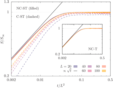
Figure 2: Growth of the entanglement entropy divided by the saturation value $S/S_{\infty}$ as a function of $t/L^{2}$ for random free fermions $-$ NC-ST (filled), C-ST (dashed) and NC-T (inset) $-$ with $L=100$ and a subsystem of $50$ sites showing $S(t)\propto\sqrt{t}$ at the earliest times. The data results from averaging over 1000 realizations up to $t=5000$, starting from a random product state with particle number fixed to $L/2$. The curves for NC-ST and NC-T overlap.

Dynamics of Entanglement $-$ For completeness, we start by analysing the dynamics of the von Neumann entropy, $S=-\operatorname{tr}(\tilde{\rho}\ln\tilde{\rho})$, with $\tilde{\rho}$ the reduced density matrix of a subsystem of size $L/2$, starting from an initial product state with a well defined particle number. Fig. 2 shows that for the three processes the entanglement grows as $\sim D_{S}\sqrt{t}$ (with $D_{S}$ a time independent constant) for small times saturating at times $t_{\rm sat}\sim L^{2}$. Asymptotically diffusive growth of the Rényi entropy $S_{2}$ has been discussed in the literature, coinciding with linear growth of the von Neumann entropy at least in low dimensional local Hilbert spaces in models with conserved quantities [30, 31]. In these cases, operator growth has a ballistically propagating front with diffusive growth in the rest frame of the front. The random circuit free fermion model is therefore qualitatively different to these cases. For $t\gg t_{\rm sat}$, the saturation value $S_{\infty}=s_{0}L+s_{1}+O(1/L)$, coincides with the mean entanglement entropy of a random Gaussian state [32, 33], with $s_{0}\simeq 0.193$ for all the considered free fermion processes and $s_{1}\simeq 0.085$ for the NC-ST case, well below the Page value $(s_{0}=\ln 2/2\simeq 0.346,s_{1}=-1/2)$ obtained by averaging over the full Hilbert space. These results show that the rate of increase of the entanglement is compatible with diffusion of quantum information. In addition, while the saturation entanglement has volume law scaling, free fermion dynamics cannot explore the full Hilbert space. We now turn to the signatures of free fermion dynamics in the spatial correlations.

Operator Spreading $-$ The time-ordered density-density correlator becomes trivial when averaged over temporal disorder (see Supplementary Section [29]) but $\mathcal{C}(r,t)$, introduced in Eq. (1), remains non-trivial upon averaging. We consider an average over separable initial states, which is equivalent to taking $\rho\propto 1$ in Eq. (1), i.e. the infinite temperature ensemble. In the following, we shall consider quadratic observables $\mathcal{O}_{r}=1/2\Psi^{\dagger}O_{r}\Psi$ where $\Psi\equiv(a_{1},\ldots,a_{L},a_{1}^{\dagger},\ldots,a_{L}^{\dagger})^{T}$ and $O_{r}$ is a local single-particle operator. The computation of $\mathcal{C}(r,t)$ for free fermions - in common with other correlators - can be brought into a form where the trace need only be performed over $2L\times 2L$ matrices rather than over the entire Hilbert space. One can show that the many-body correlator can be written in terms of single-body quantities as $\mathcal{C}(r,t)=1/2^{3}[C_{1}(r,t)-C_{2}(r,t)]$ where

$$C_{1}(r,t) ={\rm tr}\left[O^{2}_{0}(t)O^{2}_{r}\right],$$ (2)

$$C_{2}(r,t) ={\rm tr}\left[O_{0}(t)O_{r}O_{0}(t)O_{r}\right],$$ (3)

and $O(t)=UO(t-1)U^{\dagger}$. The general relation between the single particle and many-body TOC and OTOC is given in the Supplementary Material [29].

TOC and OTOC Numerics $-$ The TOC ($C_{1}$) and OTOC ($C_{2}$) may now be simulated efficiently by generating local pseudo-random gates $u_{r,r+1}$ and averaging the result over many realizations of the time evolution. As before, we average over initial states that are product states of definite particle number. Results for $L=100$ and $4000$ disorder realizations are shown in Fig. 1(c) for a symmetrized particle number operator $\mathcal{O}_{r}=1/2(a_{r}^{\dagger}a_{r}-a_{r}a_{r}^{\dagger})=a_{r}^{\dagger}a_{r}-1/2$. In contrast to the ballistic spreading seen in Haar-random circuits, $\overline{\mathcal{C}(r,t)}$ for random free fermions diffuses. This can be seen most clearly in Fig. 1(c) where $\overline{C_{1}}\,\sigma(t)/A$ and $\overline{C_{2}}\,\sigma(t)/A(t)$ are shown to collapse to a Gaussian with standard deviation growing respectively as $\sqrt{2t}$ and $\sqrt{t}$ at multiple fixed times, with the horizontal axis rescaled to $(r-\mu)/\sigma$. Examining the two terms $\overline{C_{1}}$ and $\overline{C_{2}}$ separately reveals that both the ordinary dynamical two-time correlator $\overline{C_{1}}$ and the true out-of-time-ordered component $\overline{C_{2}}$ are diffusive. The magnitude of $\overline{C_{1}}$ is, however, much larger than that of $\overline{C_{2}}$ at fixed time. These results are compatible with the observed $\sqrt{t}$ early time entanglement growth.

Exact Calculation of $\overline{C_{1}(r,t)}$ $-$ We now look for the origin of the diffusive behavior of $\overline{\mathcal{C}(r,t)}$ examining $\overline{C_{1}(r,t)}$ and $\overline{C_{2}(r,t)}$ in turn and proceeding analytically by computing the exact averages over the random unitaries for the NC-ST case referring to the Supplementary Section [29] for further details. In the single particle picture, we may denote states of the system by $\ket{\alpha}\equiv\ket{r_{\alpha},s_{\alpha}}\equiv\ket{2R_{r_{\alpha}}+b_{\alpha},s_{\alpha}}$, where $r_{\alpha}=0,\ldots,L-1$ runs over the sites, $s_{\alpha}\in\{p,h\}$ labels the particle-hole index; $R_{r_{\alpha}}=0,\ldots,L/2-1$ labels the pair of sites $(r_{\alpha},r_{\alpha}+1)$ and $b_{r_{\alpha}}\in\left\{0,1\right\}$ such that $r_{\alpha}=2R_{r_{\alpha}}+b_{r_{\alpha}}$. Note that the sites are acted upon by modulo $L$, due to periodic boundary conditions.

Starting with $\overline{C_{1}(r,t)}$, we use a notation in which operators are rendered as state vectors $C_{1}(r,t)=\operatorname{tr}\left[O_{0}^{2}(t)O_{r}^{2}\right]=\bra{\bra{O_{r}^{2}}}O_{0}^{2}(t)\rangle\rangle$, where $\ket{\ket{O_{r}^{2}}}\equiv\ket{\ket{O_{r}^{2}(0)}}$, $\ket{\ket{O_{r}^{2}(t)}}=\sum_{\alpha\beta}\ket{\ket{\alpha\beta}}\left\langle\alpha\left|O_{r}^{2}(t)\right|\beta\right\rangle$ and $\ket{\ket{\alpha\beta}}=\ket{\alpha}\otimes\bra{\beta}^{T}$. Since $O_{r}$ is the symmetrized number operator, we get

$$\ket{\ket{O_{r}^{2}}}=\sum_{s}\ket{\ket{r,s;r,s}}.$$ (4)

For a single realization, $O_{0}^{2}(t+1)=U^{\dagger}O_{0}^{2}(t)U$, which translates to $\ket{\ket{O_{0}^{2}(t+1)}}=U^{\dagger}\otimes U^{T}\ket{\ket{O_{0}^{2}(t)}}$. Applying one layer of our circuit, i.e. $U=U_{\rm{even}}U_{\rm{odd}}$, and averaging over multiple realizations of the random circuit as summarized in the Supplementary Section one finds

$$\ket{\ket{\overline{O_{0}^{2}(t+1)}}}=\hat{W}_{1}\ket{\ket{\overline{O_{0}^{2}(t)}}}$$

$$\hat{W}_{1}\equiv\left(\sum_{R=0}^{L/2-1}\ket{\ket{\phi_{2R}}}\bra{\bra{\phi_{2R}}}\right)\left(\sum_{R=0}^{L/2-1}\ket{\ket{\phi_{2R-1}}}\bra{\bra{\phi_{2R-1}}}\right),$$ (5)

having introduced

$$\ket{\ket{\phi_{r}}}\equiv\frac{1}{2}\sum_{x\in\left\{r,r+1\right\}}\sum_{s}\ket{\ket{x,s;x,s}}.$$ (6)

With the initial condition $\ket{\ket{\overline{O_{0}^{2}(0)}}}=\sum_{s}\ket{\ket{0,s;0,s}}$, the complete time evolution of $\overline{C_{1}}$ is determined. The subspace spanned by ${\ket{\ket{\phi_{r}}}}$ is closed under the evolution thus respecting the particle-hole symmetry. These vectorized operators have the property $\left\langle\left\langle\phi_{r}\right.\left\|\phi_{r^{\prime}}\right\rangle\right\rangle=\delta_{r^{\prime},r}+\frac{1}{2}\delta_{r^{\prime},r\pm 1}$ that leads to the simplification of the recursion relation, Eq. (5), to

$$\left\langle\left\langle\phi_{r}\right.\left\|\overline{O_{0}^{2}(t+1)}\right\rangle\right\rangle$$

$$=\frac{1}{4}\Big{(}\bra{\bra{\phi_{r-2}}}+2\bra{\bra{\phi_{r}}}+\bra{\bra{\phi_{r+2}}}\Big{)}\ket{\ket{\overline{O_{0}^{2}(t)}}}.$$ (7)

From this and the initial condition we obtain

$$\overline{C_{1}\left(2R,t+1\right)}=\overline{C_{1}\left(2R+1,t+1\right)}$$

$$\frac{1}{4}\big{(}\overline{C_{1}\left(2R-2,t\right)}+2\overline{C_{1}\left(2R,t\right)}+\overline{C_{1}\left(2R+2,t\right)}\Big{)}$$ (8)

for $t\geq 1$ and $\frac{1}{2}(\delta_{R-1,0}+\delta_{R,0})$ for $t=0$. Taking the continuum limit, $\lim_{t,L\rightarrow\infty}\overline{C_{1}(r,t)}=\lim_{a\rightarrow 0}a\overline{C^{\prime}_{1}(x=ra,\tau=ta^{2})}$, leads to the 1D diffusion equation $\partial_{\tau}\overline{C^{\prime}_{1}(x,\tau)}=\partial_{x}^{2}\overline{C^{\prime}_{1}(x,\tau)}$ with diffusion constant $D=1$ which approximates the exact discrete time evolution very well even for relatively small times.

Exact Calculation of $\overline{C_{2}(r,t)}$ $-$ The calculation of $\overline{C_{2}(r,t)}$ proceeds analogously to that of $\overline{C_{1}(r,t)}$ but is more involved not least because the disorder average is carried out over a product of four unitaries rather than two in the case of $\overline{C_{1}}$. As before, we write the correlator in a vectorized notation

$$C_{2}(r,t) =\operatorname{tr}\left[O_{0}(t)O_{r}O_{0}(t)O_{r}\right]=\bra{\bra{Q_{r}}}S\ket{\ket{Q_{0}(t)}},$$ (9)

with $Q_{r}\equiv O_{r}\otimes O_{r}$ fixed by the choice of observable to be

$$\ket{\ket{Q_{r}}} =\sum_{s}\ket{\ket{rs,rs,rs,rs}}-\ket{\ket{rs,r\bar{s},rs,r\bar{s}}}.$$ (10)

with $s=p,h$ and the corresponding $\bar{s}=h,p$ and

$$\ket{\ket{Q_{r}(t)}} =\sum_{\alpha\beta\mu\nu}\ket{\ket{\alpha\beta\mu\nu}}\left\langle\alpha\beta\left|Q_{r}(t)\right|\mu\nu\right\rangle,$$ (11)

$$S =\sum_{\alpha\beta\mu\nu}\ket{\ket{\alpha\beta\mu\nu}}\bra{\bra{\alpha\beta\nu\mu}},$$ (12)

where $\ket{\ket{\alpha\beta\mu\nu}}=\ket{\alpha\beta}\otimes\bra{\mu\nu}^{T}$. The $\ket{\ket{Q_{0}(t)}}$ state evolves as

$$\ket{\ket{Q_{0}(t+1)}} =U^{\dagger}\otimes U^{\dagger}\otimes U^{T}\otimes U^{T}\ket{\ket{Q_{0}(t)}}$$ (13)

and an average is taken over different realizations eventually leading to the recursion relation

$$\left\langle\left\langle\Theta\bar{\Theta}_{r,r^{\prime}}\right.\left\|\overline{Q_{0}(t+1)}\right\rangle\right\rangle=\hat{W}_{2}\ket{\ket{\overline{Q_{0}(t)}}},$$ (14)

$$\hat{W}_{2}\equiv{\rm tr}\left[\bm{M}_{r,r^{\prime}}\bm{\Upsilon}_{r,r^{\prime}}\right],$$

$$\bm{\Upsilon}_{r,r^{\prime}}\equiv\begin{pmatrix}\bra{\bra{\Theta\bar{\Theta}_{r-2,r^{\prime}-2}}}&\bra{\bra{\Theta\bar{\Theta}_{r-2,r^{\prime}}}}&\bra{\bra{\Theta\bar{\Theta}_{r-2,r^{\prime}+2}}}\\ \bra{\bra{\Theta\bar{\Theta}_{r,r^{\prime}-2}}}&\bra{\bra{\Theta\bar{\Theta}_{r,r^{\prime}}}}&\bra{\bra{\Theta\bar{\Theta}_{r,r^{\prime}+2}}}\\ \bra{\bra{\Theta\bar{\Theta}_{r+2,r^{\prime}-2}}}&\bra{\bra{\Theta\bar{\Theta}_{r+2,r^{\prime}}}}&\bra{\bra{\Theta\bar{\Theta}_{r+2,r^{\prime}+2}}}\end{pmatrix},$$

analogous to Eq. (7). In the above expression, $\bm{M}_{r,r^{\prime}}$ are $3\times 3$ matrices of constant coefficients given explicitly in the Supplementary Section. There are four distinct $\bm{M}_{r,r^{\prime}}$ for $r^{\prime}=r,r\pm 2,r\pm 4$ and one for all remaining $r^{\prime}$. The

$$\ket{\ket{\Theta\bar{\Theta}_{r,r^{\prime}}}}=\ket{\ket{\Theta_{r,r^{\prime}}}}-\ket{\ket{\bar{\Theta}_{r,r^{\prime}}}},$$ (15)

and

$$\ket{\ket{\Theta_{r,r^{\prime}}}} =\frac{1}{\sqrt{g_{r,r^{\prime}}}}\sum_{\begin{subarray}{c}r_{\alpha}\in\{r,r+1\}\\ r_{\beta}\in\{r^{\prime},r^{\prime}+1\}\end{subarray}}\sum_{s_{\alpha},s_{\beta}}\ket{\ket{\alpha\beta\beta\alpha}},$$ (16)

$$\ket{\ket{\bar{\Theta}_{r,r^{\prime}}}} =\frac{1}{\sqrt{g_{r,r^{\prime}}}}\sum_{\begin{subarray}{c}r_{\alpha}\in\{r,r+1\}\\ r_{\beta}\in\{r^{\prime},r^{\prime}+1\}\end{subarray}}\sum_{s_{\alpha},s_{\beta}}\ket{\ket{\alpha\bar{\alpha}\beta\bar{\beta}}},$$ (17)

with $g_{r,r^{\prime}}=N(N-\delta_{r,r^{\prime}})$. This completely determines the evolution of the single particle OTOC. With the initial condition, Eq. (10), one finds

$$\overline{C_{2}(r,t=0)} =2\delta_{r,0},$$ (18)

$$\overline{C_{2}(r,t=1)} =\frac{1}{18}\left(\delta_{r,-1}+\delta_{r,0}\right),$$ (19)

and, for subsequent times, we define

$$K_{r,r^{\prime}}(t)\equiv\frac{1}{2\sqrt{3}}\left\langle\left\langle\Theta\bar{\Theta}_{r,r^{\prime}}\right.\left\|\overline{Q_{0}(t)}\right\rangle\right\rangle,$$ (20)

and use Eq. (14) to get $\overline{C_{2}(2R,t+1)}=\overline{C_{2}(2R+1,t+1)}$ $={\operatorname{tr}}\left[\bm{M}_{2R,2R^{\prime}}\bm{K}_{2R,2R^{\prime}}(t)\right]$ with

$$\bm{K}_{2R,2R^{\prime}}(t)\equiv\begin{pmatrix}K_{2R-2,2R^{\prime}-2}&K_{2R-2,2R^{\prime}}&K_{2R-2,2R^{\prime}+2}\\ K_{2R,2R^{\prime}-2}&K_{2R,2R^{\prime}}&K_{2R,2R^{\prime}+2}\\ K_{2R+2,2R^{\prime}-2}&K_{2R+2,2R^{\prime}}&K_{2R+2,2R^{\prime}+2}\end{pmatrix}.$$ (21)

The evolution thus described exactly reproduces the numerical results described above. We may now take the continuum limit from Eq. (21). This highlights one important distinction between the $\overline{C_{1}}$ and $\overline{C_{2}}$ cases: the evolution of $\overline{C_{2}}$ depends on the matrix $\bm{K}$ whose elements are indexed by a pair of spatial coordinates. In the continuum limit $\overline{C_{2}(r,t)}=\lim_{a\rightarrow 0}\overline{C^{\prime}_{2}(x=ra,\tau=ta^{2})}\simeq fa^{2}K^{\prime}_{x,x^{\prime}}(\tau)$, where $K^{\prime}_{x,x^{\prime}}(\tau)$ can be shown to obey the 2D diffusion equation $\partial_{\tau}K^{\prime}_{x,x^{\prime}}(\tau)=\left(\partial_{x}^{2}+\partial_{x^{\prime}}^{2}\right)K^{\prime}_{x,x^{\prime}}(\tau)$ with initial condition $K^{\prime}_{x,x^{\prime}}(0)=2\delta(x)\delta(x^{\prime})$ and $f=1/2$ for NC-ST [29]. Note that $\lim_{t\rightarrow\infty}\overline{C_{2}(r,t)}/\overline{C_{1}(r,t)}=0$, i.e. for large times the $\overline{C_{1}(r,t)}$ dictates the leading behavior of the OTOC.

Extensions to C-ST, NC-T and NC-S $-$ We have shown that both $\overline{C_{1}}$ and $\overline{C_{2}}$ spread diffusively for free fermions in 1D in the presence of spatio-temporal noise (NC-ST). We now consider exact calculations for two further cases: C-ST where the fermion particle number is conserved and each gate in the quantum circuit is chosen randomly, and NC-T where the unitary evolution is spatially homogeneous but where there is temporal noise $-$ a single gate is chosen randomly at each time step and applied to all pairs of sites. Fig. 2 shows that the von Neumann entropy grows like $\sqrt{t}$ for all three cases: NC-ST, C-ST, NC-T. The Supplementary Section lays out in detail exact calculations of $\overline{C_{1}}$ and $\overline{C_{2}}$, analogous to the calculation summarized above for NC-ST, but with the continuum limit of $\overline{C_{2}}$ for C-ST having a different normalization due to $f=2$. The result is that there is diffusive spreading in all three cases with diffusion constants coinciding with those found for NC-ST. In contrast, numerical results obtained for the temporal homogeneous case, NC-S, presented in [29], where even and odd layers of random gates are fixed and applied repeatedly in time, show that $\overline{C_{1}}$ and $\overline{C_{2}}$ remain Anderson localized, decaying exponentially around $r=0$ [34].

Conclusions $-$ There is evidence that Hamiltonian models of quadratic fermions in one dimension exhibit diffusive spreading of correlations when subjected to noise [28, 35]. Here we have found an analytically solvable instance of this physics in the OTOC of a random circuit model with both number conserving and non-conserving quadratic fermionic terms. In the long time limit, the states that result from this dynamics are extended with volume law entanglement but depart significantly from random matrix eigenstates. In contrast, previously studied random unitary circuit models exhibit ballistic spreading of correlations with entanglement approaching the Page value asymptotically. All at once, this strongly suggests that, in Hamiltonian models of free fermions, Anderson localization is destroyed by the coherent noise we have considered and that ballistic propagation, expected for spatially homogeneous systems, becomes diffusive in the presence of noise. Both implications lay bare unusual features of quadratic fermion systems.

See pages 1 of supplement.pdf

See pages 2 of supplement.pdf

See pages 3 of supplement.pdf

See pages 4 of supplement.pdf

See pages 5 of supplement.pdf

See pages 6 of supplement.pdf

See pages 7 of supplement.pdf

See pages 8 of supplement.pdf

See pages 9 of supplement.pdf

See pages 10 of supplement.pdf

See pages 11 of supplement.pdf

See pages 12 of supplement.pdf

See pages 13 of supplement.pdf

See pages 14 of supplement.pdf

See pages 15 of supplement.pdf

See pages 16 of supplement.pdf

See pages 17 of supplement.pdf

See pages 18 of supplement.pdf

See pages 19 of supplement.pdf

See pages 20 of supplement.pdf

See pages 21 of supplement.pdf

See pages 22 of supplement.pdf

See pages 23 of supplement.pdf

See pages 24 of supplement.pdf

See pages 25 of supplement.pdf