Gradient catastrophe of nonlinear photonic valley-Hall edge pulses

Abstract

We derive nonlinear wave equations describing the propagation of slowly-varying wavepackets formed by topological valley-Hall edge states. We show that edge pulses break up even in the absence of spatial dispersion due to nonlinear self-steepening. Self-steepening leads to the previously-unattended effect of a gradient catastrophe, which develops in a finite time determined by the ratio between the pulse’s nonlinear frequency shift and the size of the topological band gap. Taking the weak spatial dispersion into account results then in the formation of stable edge quasi-solitons. Our findings are generic to systems governed by Dirac-like Hamiltonians and validated by numerical modeling of pulse propagation along a valley-Hall domain wall in staggered honeycomb waveguide lattices with Kerr nonlinearity.

The combination of topological band structures with mean field interactions not only gives rise to rich nonlinear wave physics Smirnova2020APR ; Saxena2020 , but is also anticipated to unlock advanced functionalities, such as magnet-free nonreciprocity Chen2018 , tunable and robust waveguiding Dobrykh2018 ; Shalaev2019 , and novel sources of classical and quantum light Kruk2018 ; Smirnova2018 ; Mittal2018 ; Wang2019 ; Zeng2020 ; Lan2020 . Valley-Hall photonic crystals Ma2016 ; Chen2017 ; Dong2017 ; Wu2017 ; Noh2018 ; Ni2018b ; Chen2018b ; Kang2018 ; Gao2018 ; Shalaev2018NatNano ; He2018 ; Smirnova2020LiSA ; Yang2020_Terahertz show great promise for these applications, due to their ability to combine slow-light enhancement of nonlinear effects with topological protection against disorder, which limits the performance of conventional photonic crystal waveguides Rechtsman2019 ; Sauer2020 ; Arregui2021 .

Accurate modelling of pulse propagation through photonic crystal waveguides in the slow light regime requires taking into account the dispersion in the effective nonlinearity strength, which can induce effects such as pulse self-steepening and supercontinuum generation Anderson1983 ; Panoiu2009 ; Travers2011 ; Husko2015 . Despite the proven importance of these effects in applications Kivshar_book ; Soljacic2004 ; RevModPhys.78.1135 , analysis of nonlinear light propagation in topological photonic structures most often assumes non-dispersive nonlinearities, in both the underlying material response Plotnik2013 ; Kartashov2016 ; Leykam2016 ; Solnyshkov2017 ; Zhang2019 ; Tulop2020 ; Chaunsali2021 ; Guo2020 ; Xia2020 ; Mukherjee2020 ; Maczewsky2020 and effective models describing the propagation of nonlinear edge states Ablowitz2013 ; Ablowitz2014 ; Lumer2016 ; Ivanov2020 ; Ivanov2020b . The simplest effective model is the cubic nonlinear Schrödinger equation (NLSE), which describes the self-focusing dynamics of edge wavepackets independent of the properties of the topological band gap, such as its size.

More sophisticated effective models such as nonlinear Dirac models explicitly include the nontrivial spin-like degrees of freedom required to create topological band gaps Maravero2016 ; Bomantara2017 ; Sakaguchi2018 ; RingSoliton2018 ; Smirnova2019LPR . In the bulk, the nonlinear Dirac model supports self-induced domain walls and solitons whose stability and degree of localization are sensitive to the gap size. Infinitely-extended (plane wave-like) nonlinear edge states can be obtained analytically and exhibit similar features. However, the nonlinear dynamics of localized edge pulses within the nonlinear Dirac model framework were not yet considered.

In this paper we study an analytically-solvable nonlinear Dirac model (NDM) describing topological edge pulses, revealing that nonlinear topological edge states’ exhibit a self-steepening nonlinearity when the pulse self-frequency modulation becomes comparable to the width of the topological band gap. The self-steepening nonlinearity leads to the formation of a gradient catastrophe of edge wavepackets within a finite propagation time proportional to the pulse width. Taking the weak spatial dispersion of the topological edge modes into account regularizes the catastrophe and results in the formation of stable edge solitons for sufficiently long pulses. We validate our analysis using numerical simulations of beam propagation in a laser-written valley-Hall waveguide lattice, demonstrating that this effect should be observable even for relatively weak nonlinearities. Our findings suggest valley-Hall photonic crystal waveguides will provide a fertile setting for observing and harnessing higher-order nonlinear optical effects.

We consider a generic continuum Dirac model of topological photonic lattices with incorporated nonlinear terms. The evolution of a spinor wavefunction ${\bf{\Psi}}(x,y,t)=[\Psi_{1}(x,y,t);\Psi_{2}(x,y,t)]^{T}$ in the vicinity of a band crossing point (topological phase transition) is governed by the nonlinear Dirac equation Maravero2016 ; RingSoliton2018 ; Smirnova2019LPR

$$i\partial_{t}{\bf{\Psi}}=\left(\hat{H}_{D}(\delta{\bf{k}})+\hat{H}_{N\!L}\right){\bf{\Psi}};$$ (1)

$$\hat{H}_{D}(\delta{\bf{k}})=\delta k_{x}\hat{\sigma}_{x}+\delta k_{y}\hat{\sigma}_{y}+M\hat{\sigma}_{z},$$ (2)

where $\delta{\bf{k}}=\left(\delta k_{x},\delta k_{y}\right)\equiv-i\left(\partial_{x},\partial_{y}\right)$ is the momentum, $M$ is a detuning between two sublattices or spin states, and $\hat{H}_{N\!L}=-g\,\mathrm{diag}[\left|\Psi_{1}\right|^{2};\left|\Psi_{2}\right|^{2}]$ is a local non-dispersive Kerr nonlinearity.

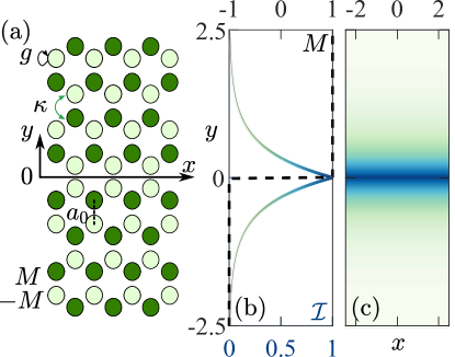
Figure 1: (a) Dimerized photonic graphene lattice with staggered sublattice potential. Here $\kappa$ denotes the tunneling coefficient between waveguides, $a_{0}$ is the distance between neighboring waveguides, and the round arrow $g$ illustrates the nonlinear self-action effect. (b) Transverse profile $\mathcal{I}(y)$ and (c) in-plane intensity distribution $\mathcal{I}(x,y)=|\psi_{1}(x,y)|^{2}+|\psi_{2}(x,y)|^{2}$ of the nonlinear edge wave propagating along the $x$ axis and bound to the domain wall located at $y=0$, where the effective mass $M(y)$ changes sign. Parameters are $M_{0}=1,~{}g=0.75$.

As a specific example, the model (1) can be implemented in nonlinear photonic graphene with a staggered sublattice potential as illustrated in Fig. 1(a). A dimerized graphene lattice is composed of single-mode dielectric waveguides with local Kerr nonlinearity. The effective mass $M$ characterises a detuning between propagation constants in the waveguides of two sublattices. The form of Hamiltonian operator (2) assumes normalization of the transverse coordinates $x,y$ and evolution variable in the propagation direction $t\sim z/v_{D}$ to the Dirac velocity $v_{D}=3\kappa a_{0}/2$ defined by the lattice parameters, a coupling constant $\kappa$ and a distance $a_{0}$ between two neighboring waveguides Smirnova2019LPR ; Smirnova2020LiSA . This continuum model is valid provided $|\kappa|\gtrsim 2|M|$ Smirnova2020LiSA .

The valley-Hall domain wall is created between two insulators characterized by different signs of the mass. We take $M(y>0)=M_{0}$ and $M(y<0)=-M_{0}$ and without loss of generality assume $M_{0}>0$ in the upper half-space. In Ref. Smirnova2019LPR we derived exact analytic solutions for the propagating nonlinear valley edge modes bound to the interface $y=0$: ${\bf{\Psi}}(y,x,t)=[\psi_{1}^{0}(y,\omega,k);\psi_{2}^{0}(y,\omega,k)]^{T}e^{ikx-i\omega t}$. Based on the close connections between nonlinear edge states and self-trapped Dirac solitons in topological band gaps revealed in Ref. Smirnova2019LPR , the nonlinear edge mode dispersion can be obtained as

$$\omega+k=-g\mathcal{I}_{1}/2$$ (3)

with the transverse profile of the edge state determined by the intensity at the interface $\mathcal{I}_{1}=|\psi_{1,2}(y=0)|^{2}$ (see Supplemental Material Suppl ). In Figs. 1(b,c) we show the plane wave-like profile of the nonlinear edge mode with fixed wavenumber $k$ parallel to the edge.

Using the global parity symmetry with respect to the interface and analytical solutions for the edge states Suppl , we calculate two characteristics of the edge states via integration in the upper half plane $y>0$: the power $\mathcal{P}$ and spin ${{S}}_{x}$,

$${\mathcal{P}}=\int_{0}^{\infty}{\bm{\psi}}^{\dagger}{\bm{\psi}}dy,\quad{{S}}_{x}=\frac{1}{2}\int_{0}^{\infty}{{\bm{\psi}}^{\dagger}\hat{\sigma}_{x}{\bm{\psi}}}dy\>,$$ (4)

and identify a functional relation ${{S}}_{x}\left({\mathcal{P}}\right)$ between them:

$${{S}}_{x}=-\frac{1}{g}\arcsin\left[\frac{1}{\sqrt{2}}\sin\left({\mathcal{P}}\frac{g}{\sqrt{2}}\right)\right]\>.$$ (5)

Crucially, this relation is independent of the wavevector $k$, which allows us to develop a slowly varying envelope approximation to describe the nonlinear dynamics of finite edge wavepackets. Using Eq. (1), it can be shown that the integral characteristics obey the following evolution equation:

$${\partial}_{t}\mathcal{P} =-2{\partial}_{x}{S_{x}}(\mathcal{P}).$$ (6)

Next, we assume $\mathcal{P}(x,t)$ and $S_{x}(x,t)$ are slowly varying functions of the local frequency and wavenumber, such that Eq. (5) remains valid to a first approximation for smooth $x$-dependent field envelopes. Plugging Eq. (5) into Eq. (6), and using Eq. (3) assuming weak nonlinearity $g\mathcal{I}_{1}\ll M_{0}$, we obtain the simple nonlinear wave equation for the longitudinal intensity profile $\mathcal{I}_{1}(x,t)$:

$$\partial_{t}\mathcal{I}_{1}-\partial_{x}\mathcal{I}_{1}\left(1-g^{2}\mathcal{I}_{1}^{2}/\left(4M_{0}^{2}\right)\right)=0.$$ (7)

Equation (7) suggests that the evolution of finite wavepackets propagating along the $x$ axis is accompanied by steepening of the trailing wavefront up to the development of a gradient catastrophe. Note, in the linear case $g=0$, Eq. (7) shows that the edge wavepacket of any shape does not diffract and propagates along the domain wall with constant group velocity $v=-1$, being granted with topological robustness. Alternatively, Eq. (7) can be derived using asymptotic methods based on a series expansion of the spinor wavefunction Suppl

$$\Psi_{1,2}(x,y,t)=\pm a(\xi;\tau_{n})e^{-M_{0}|y|}+\sum_{n=1}^{\infty}\mu^{n}\Psi_{1,2}^{(n)}\left(y;\xi;\tau_{n}\right)\>,$$ (8)

where we have introduced a small parameter $\mu\sim{g\mathcal{I}_{1}}/{M_{0}}$, a hierarchy of time scales: $\tau_{n}=\mu^{n}t$, and assumed a smooth dependence of the spinor components on $t$ in the moving coordinate frame $(\xi\equiv x+t,y)$.

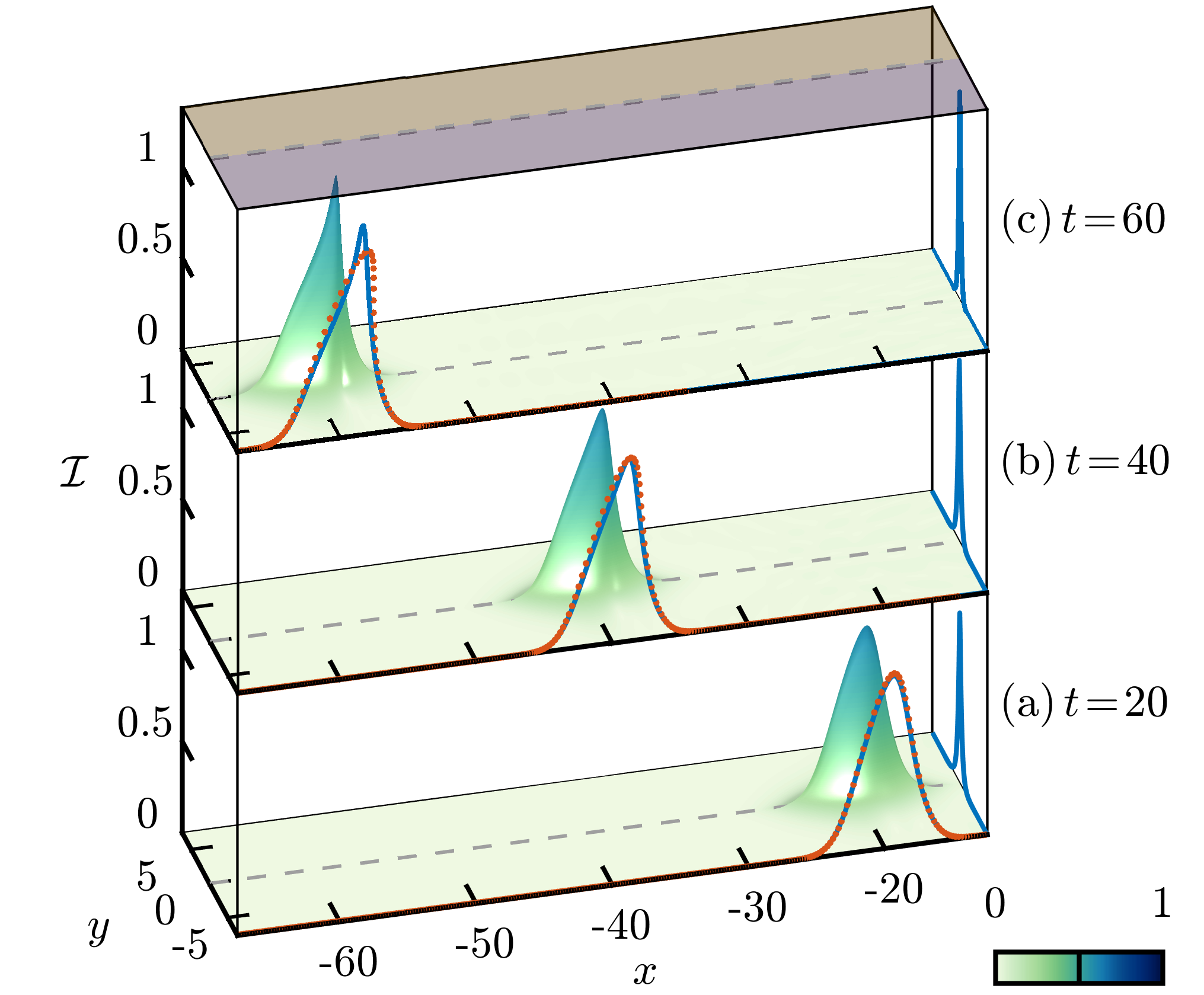
Figure 2: Gradient catastrophe development. The Gaussian pulse with $F_{0}=1$, $\Lambda_{0}=3.5$ is launched at $t=0$. Slices color code intensity distributions $\mathcal{I}(x,y)$ at the given moments: (a) $t=20$, (b) $t=40$, (c) $t=60$. Cuts along the domain wall at $y=0$ show consistency of the numerical solution (blue curves) with the solution of the nonlinear simple wave equation (7) for the intensity (red dotted lines). Parameters are $M_{0}=1$, $g=0.75$. In Figs. 2, 3, dashed lines trace the domain wall separating spatial domains with masses of the opposite sign as indicated by shading with different colors on the top surface.

To illustrate the key effect of the gradient catastrophe captured by Eq. (7), we model the time dynamics of an edge wavepacket using a custom numerical code, applying a split-step scheme and the fast Fourier transform to solve Eq. (1). Figure 2 shows evolution of the initial distribution set in the form of the edge state across the interface with the Gaussian envelope $\mathcal{I}_{1}^{0}(x,t=0)=F_{0}e^{-x^{2}/\Lambda_{0}^{2}}$ along the $x$ axis: $\bm{\psi}(y,x,t=0)=\left[\psi_{1}^{0}\left(y,\omega=-{g\mathcal{I}^{0}_{1}\left(x\right)}/{2},0\right);\psi_{2}^{0}\left(y,\omega=-{g\mathcal{I}^{0}_{1}\left(x\right)}/{2},0\right)\right]^{T}$. Plugging the Gaussian distribution into Eq. (7), we may estimate the pulse breakdown time $t_{*}$ analytically:

$$t_{*}=2\sqrt{e}\Lambda_{0}\left(\displaystyle\frac{M_{0}}{gF_{0}}\right)^{2}.$$ (9)

Thus, pulse breakdown occurs for finite wavepackets when the peak nonlinear frequency shift becomes comparable to the size of the topological band gap. As the pulse propagates its tail becomes increasingly steep, developing a discontinuity (i.e. a shock) in a finite time. The numerical solution of Eq. (1) is fully consistent with our analytical considerations, see Fig. 2.

Weak spatial dispersion effects serve as a possible mechanism regularizing the gradient catastrophe, resulting in the formation of solitons. For honeycomb photonic lattices, dispersion is accounted for by introducing off-diagonal second-order derivatives with the coefficient $\eta=(6\kappa)^{-1}$ into the Dirac model (1):

$$\hat{H}_{\text{disp}}\!=\left(\!{\begin{array}[]{*{22}{c}}{0}&{-\eta\left(-i\partial_{x}+\partial_{y}\right)^{2}}\\ {-\eta\left(i\partial_{x}+\partial_{y}\right)^{2}}&{0}\end{array}}\!\right).$$ (10)

Assuming $\eta M_{0}\sim\mu^{2}$ and developing a perturbation theory with expansion (8), we derive an evolution equation governing the complex-valued amplitude $a(\xi,t)$:

$$i\left({\partial_{t}a}+\displaystyle\frac{g^{2}|a|^{2}}{32M_{0}^{2}}{a{\partial_{\xi}}|a|^{2}}\right)+\displaystyle\frac{g}{4}|a|^{2}a+\eta\left({\partial_{\xi^{2}}}a-M_{0}^{2}a\right)=0\>,$$ (11)

which differs from the conventional cubic nonlinear Schrödinger equation by the second higher-order nonlinear term responsible for the phase modulation and self-steepening. This equation enables analysis of both the modulational instability of nonlinear plane-wave-like edge states, and the formation of edge quasi-solitons Suppl .

To verify the validity of the modified NLSE (11) we consider the propagation of a Gaussian pulse in Fig. 3. The conventional NLSE, which lacks the self-steepening term, only exhibits self-focusing and gradual self-compression of the pulse. On the other hand, the modified Eq. (11) correctly reproduces the growing asymmetry of the edge pulse as it propagates. We show in the Supplemental Material how the self-steepening leads to the break-up of wide pulses, resulting in the radiation of part of its energy into bulk modes, with the remainder forming a quasi-soliton which continues to propagate along the edge and is capable of traversing sharp bends. We note that even after the initial pulse breakup, self-steepening terms can influence the soliton stability and soliton-soliton interactions Kivshar_book .

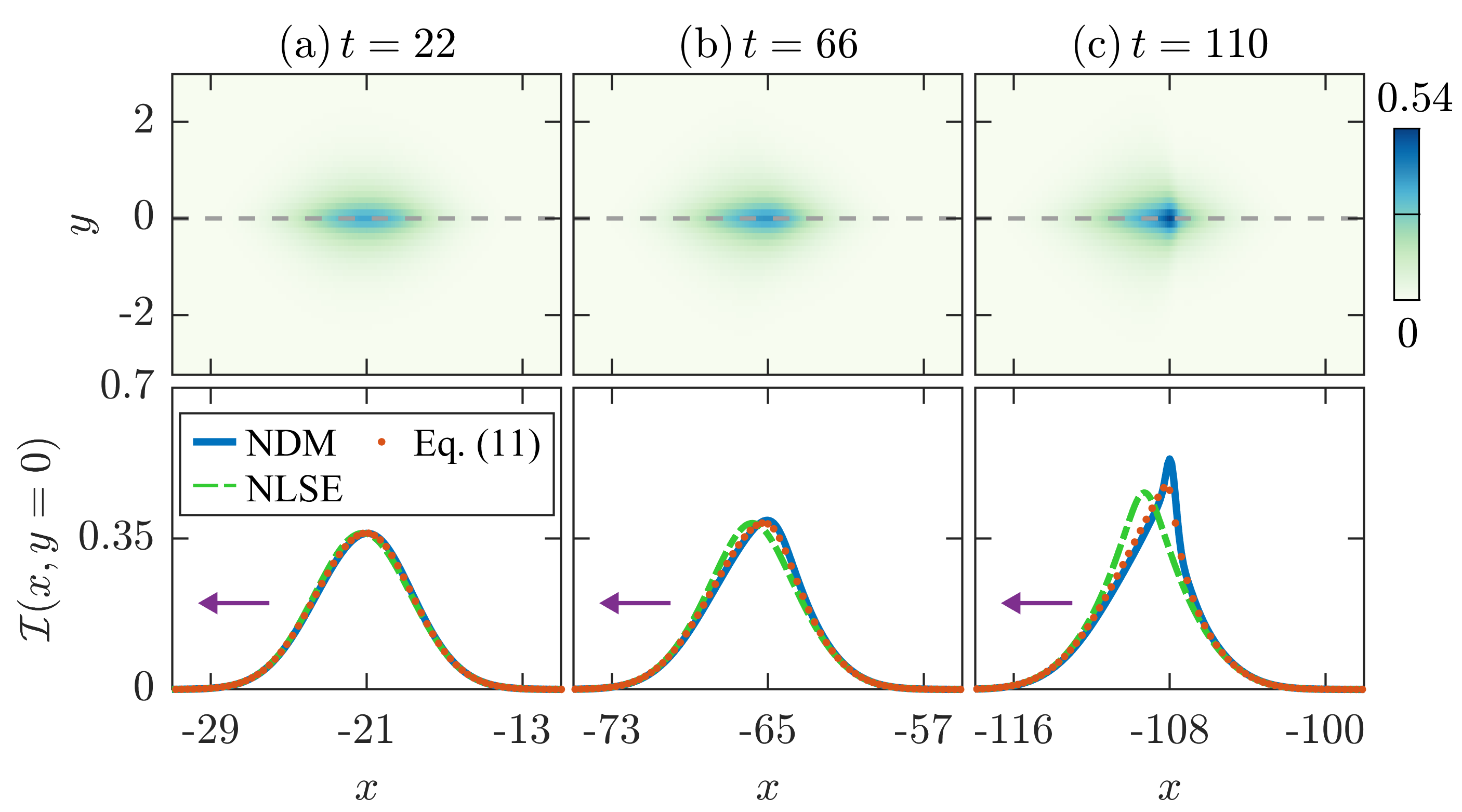
Figure 3: Nonlinear pulse transformation in the domain-wall problem with dispersion. Snapshots show intensity distributions in-plane $\mathcal{I}(x,y)$ (top row) and along the domain wall $\mathcal{I}(x,y=0)$ (bottom row) at the given times: (a) $t=22$, (b) $t=66$, (c) $t=110$. Overlaid curves are the pulse envelopes calculated by using NLSE (green dashed) and Eq. (11) (red dotted). The Gaussian pulse with $F_{0}=0.18$, $\Lambda_{0}=5/\sqrt{2}$ is launched at $t=0$. Parameters are $M_{0}=1$, $g=1$, $\eta=0.001$.

As a possible implementation, we consider a realistic valley-Hall waveguide array of laser-written waveguides with parameters similar to those used in the experimental work Ref. Noh2018 . In this case, the evolution variable $t$ becomes the longitudinal propagation distance $z$. To simulate the evolution, we solve the paraxial equation numerically in a periodic potential by propagating an optical wavepacket Suppl . For realistic laser input powers we observe a notable distortion of the beam and signatures of the catastrophe development at its trailing wavefront [Fig. 4(a,b)]. Figure 4(c) plots the intensity map in $xz$ interface plane. The rapidly developing asymmetry at short distances agrees with modeling of the corresponding continuum Dirac equations and estimates of the breakdown coordinate $z_{*}$ based on Eq. (9) [Fig. 4(d)].

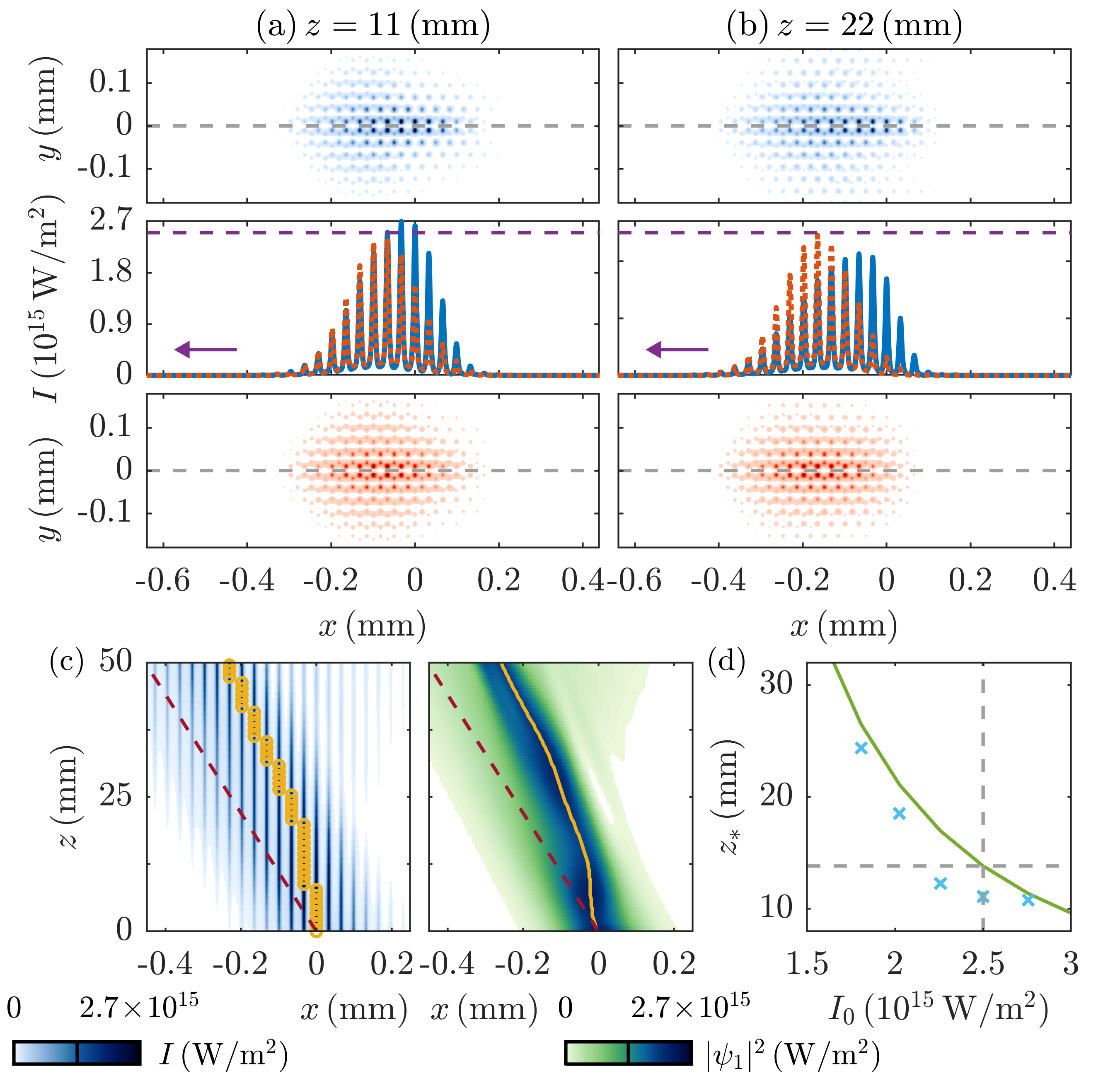
Figure 4: Nonlinear dynamics of the optical beam at the valley-Hall domain wall at a zigzag interface in a honeycomb lattice of laser-written waveguides. The input beam has Gaussian envelope along the domain wall with maximum intensity $I_{0}=2.5\times 10^{15}$ W/m². (a,b) Intensity distributions of the nonlinear beam (top panels, blue line) at propagation distances (a) $z=11$ mm (left column) and (b) $z=22$ mm (right column). For comparison, the linear beam evolution, i.e. with nonlinearity switched off, is shown on bottom panels and with dotted red lines. Purple arrows points to the direction of motion. Dashed grey line depicts the domain wall. (c) Intensity distribution at the interface obtained in modeling of the paraxial equation (left) and the corresponding Dirac model (right). The purple dashed line traces a straight trajectory of the center of mass of the linear pulse. (d) Breakdown coordinate $z_{*}$ as a function of the input intensity $I_{0}$ estimated from the Dirac model (green curve) and paraxial modeling (cyan crosses). The dashed grey lines’ intersection indicates the value of the input beam intensity used for (a,b,c).

In conclusion, we have described the gradient catastrophe of the nonlinear edge wavepackets in the spinor-type Dirac equation and the formation of edge solitons at the valley-Hall domain walls. We have derived a higher-order self-steepening nonlinear Schrödinger equation describing these effects. Spatiotemporal numerical modeling confirmed that pulse self-steepening can manifest already in the framework of paraxial optics in weakly nonlinear media, such as topological waveguide lattices, and will likely play a key role in future experiments with topological photonic crystal waveguides. Beyond the specific valley-Hall example we considered, our findings are instructive for other emerging experimental studies of nonlinear dynamic phenomena in topological systems, such as the Chern insulators and their implementations in a variety of physical platforms spanning from metamaterials Dobrykh2018 to optical lattices Mukherjee2020 ; Xia2020 and exciton-polariton condensates Pernet_arxiv .

- (1) D. Smirnova, D. Leykam, Y. Chong, and Y. Kivshar, “Nonlinear topological photonics,” Applied Physics Reviews 7, 021306 (2020).
- (2) A. Saxena, P. G. Kevrekidis, and J. Cuevas-Maraver, Nonlinearity and Topology (Springer International Publishing, Cham, 2020), pp. 25–54.
- (3) W. Chen, D. Leykam, Y. Chong, and L. Yang, “Nonreciprocity in synthetic photonic materials with nonlinearity,” MRS Bulletin 43, 443–451 (2018).
- (4) D. A. Dobrykh, A. V. Yulin, A. P. Slobozhanyuk, A. N. Poddubny, and Y. S. Kivshar, “Nonlinear control of electromagnetic topological edge states,” Phys. Rev. Lett. 121, 163901 (2018).
- (5) M. I. Shalaev, W. Walasik, and N. M. Litchinitser, “Optically tunable topological photonic crystal,” Optica 6, 839 (2019).
- (6) S. Kruk, A. Poddubny, D. Smirnova, L. Wang, A. Slobozhanyuk, A. Shorokhov, I. Kravchenko, B. Luther-Davies, and Y. Kivshar, “Nonlinear light generation in topological nanostructures,” Nature Nanotechnology 14, 126–130 (2019).
- (7) D. Smirnova, S. Kruk, D. Leykam, E. Melik-Gaykazyan, D.-Y. Choi, and Y. Kivshar, “Third-harmonic generation in photonic topological metasurfaces,” Phys. Rev. Lett. 123, 103901 (2019).
- (8) S. Mittal, E. A. Goldschmidt, and M. Hafezi, “A topological source of quantum light,” Nature 561, 502–506 (2018).
- (9) Y. Wang, L.-J. Lang, C. H. Lee, B. Zhang, and Y. D. Chong, “Topologically enhanced harmonic generation in a nonlinear transmission line metamaterial,” Nature Communications 10, 1102 (2019).
- (10) Y. Zeng, U. Chattopadhyay, B. Zhu, B. Qiang, J. Li, Y. Jin, L. Li, A. G. Davies, E. H. Linfield, B. Zhang, Y. Chong, and Q. J. Wang, “Electrically pumped topological laser with valley edge modes,” Nature 578, 246–250 (2020).
- (11) Z. Lan, J. W. You, and N. C. Panoiu, “Nonlinear one-way edge-mode interactions for frequency mixing in topological photonic crystals,” Phys. Rev. B 101, 155422 (2020).
- (12) T. Ma and G. Shvets, “All-Si valley-Hall photonic topological insulator,” New Journal of Physics 18, 025012 (2016).
- (13) X.-D. Chen, F.-L. Zhao, M. Chen, and J.-W. Dong, “Valley-contrasting physics in all-dielectric photonic crystals: Orbital angular momentum and topological propagation,” Phys. Rev. B 96, 020202 (2017).
- (14) J.-W. Dong, X.-D. Chen, H. Zhu, Y. Wang, and X. Zhang, “Valley photonic crystals for control of spin and topology,” Nature Materials 16, 298–302 (2017).
- (15) X. Wu, Y. Meng, J. Tian, Y. Huang, H. Xiang, D. Han, and W. Wen, “Direct observation of valley-polarized topological edge states in designer surface plasmon crystals,” Nature Communications 8, 1304 (2017).
- (16) J. Noh, S. Huang, K. P. Chen, and M. C. Rechtsman, “Observation of photonic topological valley Hall edge states,” Phys. Rev. Lett. 120, 063902 (2018).
- (17) X. Ni, D. Purtseladze, D. A. Smirnova, A. Slobozhanyuk, A. Alù, and A. B. Khanikaev, “Spin- and valley-polarized one-way Klein tunneling in photonic topological insulators,” Science Advances 4 (2018).
- (18) X.-D. Chen, F.-L. Shi, H. Liu, J.-C. Lu, W.-M. Deng, J.-Y. Dai, Q. Cheng, and J.-W. Dong, “Tunable electromagnetic flow control in valley photonic crystal waveguides,” Phys. Rev. Applied 10, 044002 (2018).
- (19) Y. Kang, X. Ni, X. Cheng, A. B. Khanikaev, and A. Z. Genack, “Pseudo-spin–valley coupled edge states in a photonic topological insulator,” Nature Communications 9, 3029 (2018).
- (20) F. Gao, H. Xue, Z. Yang, K. Lai, Y. Yu, X. Lin, Y. Chong, G. Shvets, and B. Zhang, “Topologically protected refraction of robust kink states in valley photonic crystals,” Nature Physics 14, 140–144 (2018).
- (21) M. I. Shalaev, W. Walasik, A. Tsukernik, Y. Xu, and N. M. Litchinitser, “Robust topologically protected transport in photonic crystals at telecommunication wavelengths,” Nature Nanotechnology 14, 31–34 (2018).
- (22) X.-T. He, E.-T. Liang, J.-J. Yuan, H.-Y. Qiu, X.-D. Chen, F.-L. Zhao, and J.-W. Dong, “A silicon-on-insulator slab for topological valley transport,” Nature Communications 10, 872 (2019).
- (23) D. Smirnova, A. Tripathi, S. Kruk, M.-S. Hwang, H.-R. Kim, H.-G. Park, and Y. Kivshar, “Room-temperature lasing from nanophotonic topological cavities,” Light: Science & Applications 9 (2020).
- (24) Y. Yang, Y. Yamagami, X. Yu, P. Pitchappa, J. Webber, B. Zhang, M. Fujita, T. Nagatsuma, and R. Singh, “Terahertz topological photonics for on-chip communication,” Nature Photonics 14, 446–451 (2020).
- (25) J. Guglielmon and M. C. Rechtsman, “Broadband topological slow light through higher momentum-space winding,” Phys. Rev. Lett. 122, 153904 (2019).
- (26) E. Sauer, J. P. Vasco, and S. Hughes, “Theory of intrinsic propagation losses in topological edge states of planar photonic crystals,” Phys. Rev. Research 2, 043109 (2020).
- (27) G. Arregui, J. Gomis-Bresco, C. M. Sotomayor-Torres, and P. D. Garcia, “Quantifying the robustness of topological slow light,” Phys. Rev. Lett. 126, 027403 (2021).
- (28) D. Anderson and M. Lisak, “Nonlinear asymmetric self-phase modulation and self-steepening of pulses in long optical waveguides,” Phys. Rev. A 27, 1393–1398 (1983).
- (29) N. C. Panoiu, X. Liu, and R. M. Osgood, “Self-steepening of ultrashort pulses in silicon photonic nanowires,” Opt. Lett. 34, 947–949 (2009).
- (30) J. C. Travers, W. Chang, J. Nold, N. Y. Joly, and P. S. J. Russell, “Ultrafast nonlinear optics in gas-filled hollow-core photonic crystal fibers,” J. Opt. Soc. Am. B 28, A11–A26 (2011).
- (31) C. Husko and P. Colman, “Giant anomalous self-steepening in photonic crystal waveguides,” Phys. Rev. A 92, 013816 (2015).
- (32) Y. Kivshar and G. Agrawal, Optical Solitons: From Fibers to Photonic Crystals (Elsevier, 2003).
- (33) M. Soljačić and J. D. Joannopoulos, “Enhancement of nonlinear effects using photonic crystals,” Nature Materials 3, 211–219 (2004).
- (34) J. M. Dudley, G. Genty, and S. Coen, “Supercontinuum generation in photonic crystal fiber,” Rev. Mod. Phys. 78, 1135–1184 (2006).
- (35) Y. Lumer, Y. Plotnik, M. C. Rechtsman, and M. Segev, “Self-localized states in photonic topological insulators,” Phys. Rev. Lett. 111, 243905 (2013).
- (36) Y. V. Kartashov and D. V. Skryabin, “Modulational instability and solitary waves in polariton topological insulators,” Optica 3, 1228 (2016).
- (37) D. Leykam and Y. D. Chong, “Edge solitons in nonlinear-photonic topological insulators,” Phys. Rev. Lett. 117, 143901 (2016).
- (38) D. Solnyshkov, O. Bleu, B. Teklu, and G. Malpuech, “Chirality of topological gap solitons in bosonic dimer chains,” Phys. Rev. Lett. 118, 023901 (2017).
- (39) W. Zhang, X. Chen, Y. V. Kartashov, V. V. Konotop, and F. Ye, “Coupling of edge states and topological Bragg solitons,” Phys. Rev. Lett. 123, 254103 (2019).
- (40) T. Tuloup, R. W. Bomantara, C. H. Lee, and J. Gong, “Nonlinearity induced topological physics in momentum space and real space,” Phys. Rev. B 102, 115411 (2020).
- (41) R. Chaunsali, H. Xu, J. Yang, P. G. Kevrekidis, and G. Theocharis, “Stability of topological edge states under strong nonlinear effects,” Phys. Rev. B 103, 024106 (2021).
- (42) M. Guo, S. Xia, N. Wang, D. Song, Z. Chen, and J. Yang, “Weakly nonlinear topological gap solitons in Su–Schrieffer–Heeger photonic lattices,” Opt. Lett. 45, 6466–6469 (2020).
- (43) S. Xia, D. Jukić, N. Wang, D. Smirnova, L. Smirnov, L. Tang, D. Song, A. Szameit, D. Leykam, J. Xu, Z. Chen, and H. Buljan, “Nontrivial coupling of light into a defect: the interplay of nonlinearity and topology,” Light: Science & Applications 9 (2020).
- (44) S. Mukherjee and M. C. Rechtsman, “Observation of Floquet solitons in a topological bandgap,” Science 368, 856–859 (2020).
- (45) L. J. Maczewsky, M. Heinrich, M. Kremer, S. K. Ivanov, M. Ehrhardt, F. Martinez, Y. V. Kartashov, V. V. Konotop, L. Torner, D. Bauer, and A. Szameit, “Nonlinearity-induced photonic topological insulator,” Science 370, 701–704 (2020).
- (46) M. J. Ablowitz, C. W. Curtis, and Y. Zhu, “Localized nonlinear edge states in honeycomb lattices,” Phys. Rev. A 88, 013850 (2013).
- (47) M. J. Ablowitz, C. W. Curtis, and Y.-P. Ma, “Linear and nonlinear traveling edge waves in optical honeycomb lattices,” Phys. Rev. A 90, 023813 (2014).
- (48) Y. Lumer, M. C. Rechtsman, Y. Plotnik, and M. Segev, “Instability of bosonic topological edge states in the presence of interactions,” Phys. Rev. A 94, 021801 (2016).
- (49) S. K. Ivanov, Y. V. Kartashov, A. Szameit, L. Torner, and V. V. Konotop, “Vector topological edge solitons in Floquet insulators,” ACS Photonics 7, 735–745 (2020).
- (50) S. K. Ivanov, Y. V. Kartashov, L. J. Maczewsky, A. Szameit, and V. V. Konotop, “Bragg solitons in topological Floquet insulators,” Opt. Lett. 45, 2271–2274 (2020).
- (51) J. Cuevas-Maraver, P. G. Kevrekidis, A. Saxena, A. Comech, and R. Lan, “Stability of solitary waves and vortices in a 2D nonlinear Dirac model,” Phys. Rev. Lett. 116, 214101 (2016).
- (52) R. W. Bomantara, W. Zhao, L. Zhou, and J. Gong, “Nonlinear Dirac cones,” Phys. Rev. B 96, 121406 (2017).
- (53) H. Sakaguchi and B. A. Malomed, “One- and two-dimensional gap solitons in spin-orbit-coupled systems with Zeeman splitting,” Phys. Rev. A 97, 013607 (2018).
- (54) A. N. Poddubny and D. A. Smirnova, “Ring Dirac solitons in nonlinear topological systems,” Phys. Rev. A 98, 013827 (2018).
- (55) D. A. Smirnova, L. A. Smirnov, D. Leykam, and Y. S. Kivshar, “Topological edge states and gap solitons in the nonlinear Dirac model,” Laser & Photonics Reviews 13, 1900223 (2019).
- (56) See Supplemental Material, which contains detailed derivations and additional numerical results on edge solitons and linear waveguide arrays.
- (57) N. Pernet, P. St-Jean, D. D. Solnyshkov, G. Malpuech, N. C. Zambon, B. Real, O. Jamadi, A. Lemaître, M. Morassi, L. L. Gratiet, T. Baptiste, A. Harouri, I. Sagnes, A. Amo, S. Ravets, and J. Bloch, “Topological gap solitons in a 1D non-Hermitian lattice,” arXiv p. 2101.01038 (2021).