A Data-Driven Energy Storage System-Based Algorithm for Monitoring the Small-Signal Stability of Power Grids with Volatile Wind Power

Abstract

In this paper, we propose a data-driven energy storage system (ESS)-based method to enhance the online small-signal stability monitoring of power networks with high penetration of intermittent wind power. To accurately estimate inter-area modes that are closely related to the system’s inherent stability characteristics, a novel algorithm that leverages on recent advances in wide-area measurement systems (WAMSs) and ESS technologies is developed. It is shown that the proposed approach can smooth the wind power fluctuations in near real-time using a small additional ESS capacity and thus significantly enhance the monitoring of small-signal stability. Dynamic Monte Carlo simulations on the IEEE 68-bus system are used to illustrate the effectiveness of the proposed algorithm in smoothing wind power and estimating the inter-area mode statistical properties.

I Introduction

Wind power is a rapidly evolving renewable energy technology worldwide because of its cleanness, abundance and cost-effectiveness. However, the volatile and stochastic nature of wind poses many challenges to the secure operation of modern grids. Concerning small-signal stability, the intermittency of wind energy may not only lead to instability [1] but also result in great obstacles regarding the power system stability monitoring and assessment [2]. Particularly, poorly-damped inter-area oscillations may become undetectable if small-signal stability monitoring is deteriorated. Such a phenomenon can cause major power outages [3]. Recent works have proposed probabilistic approaches to study and quantify the impact of wind power on small-signal stability analysis, which may nevertheless require large computational effort [4], [5].

The recent advances in energy storage systems (ESSs) have provided power engineers with an effective means to minimize the unwanted impacts of wind energy on power networks by smoothing wind power variations [6]. However, even with ESSs, additional challenges may arise as power grids are transforming into large-scale networks with increasing complexity, due to the continuous integration of power electronics-based devices, the transmission system expansion, etc. In fact, [7] has shown that the conventional model-based methods for small-signal stability monitoring may fail when the power system experiences unexpected disturbances or undetected topology changes. In this direction, measurement-based methods have been proposed in the recent literature to monitor and control small-signal stability considering load uncertainties [7, 8, 9, 10]. These strategies mainly rely on the enormous growth of wide-area measurement systems (WAMSs) and phasor measurement units (PMUs) over the last $10-20$ years [11]. Despite of providing advancements, these works do not consider wind stochasticity.

To address these challenges, in this paper, a novel data-driven ESS-based algorithm for monitoring the small-signal stability of power grids with volatile wind power is proposed. Our method exploits two of the key emerging technologies–WAMS and ESS–that have already been massively installed in most power networks [12], to accurately monitor the inter-area modes of systems with random renewables in near real-time. Particularly, we install ESSs at the wind generator side to smooth out the random wind power fluctuations. The assumption of having ESSs at wind generator side may be optimistic now, but is commonly made in the literature due to the fast rate of ESS deployment in power grids [6, 12, 13]. We then apply an online data-driven mode identification approach to estimate the dynamic system state matrix and the inter-area mode characteristics. Unlike probabilistic stability assessment approaches, the proposed method enables small-signal stability assessment online (within a $5$ minutes window). In addition, it will be shown that the ESS capacity required for wind power smoothing can be determined based on the statistical properties of wind farm power output, whereas its size is not significant when compared with the large scale of power grids. To the best of authors’ knowledge, this work represents the first attempt to enhance the data-driven monitoring of small-signal stability considering the stochastic nature of renewable energy sources.

II Stochastic Model for Power Grid Dynamics

Inter-area modes lie in the low-frequency portion of the electromechanical mode spectrum (i.e. $0.1-1$ Hz) [14]. Thus, fast generator dynamics can be neglected and aggregated synchronous machines can be represented by the classical model [14]. By numbering generator buses as $i=1,...,n$:

$$\dot{\delta}_{i} = \omega_{i}$$ (1)

$$M_{i}\dot{\omega}_{i} = P_{m_{i}}-P_{e_{i}}-D_{i}\omega_{i}$$ (2)

$$P_{e_{i}} = E_{i}\sum\limits_{j=1}^{n}E_{j}|Y_{i,j}|\cos(\delta_{i}-\delta_{j}-\phi_{i,j})$$ (3)

where $\delta_{i}$ is the rotor angle, $\omega_{i}$ the rotor speed deviation from synchronous speed, $M_{i}$ the inertia coefficient, $D_{i}$ the damping coefficient, $P_{m_{i}}$ the mechanical power input, $P_{e_{i}}$ the electrical power output, $E_{i}$ the transient emf magnitude, and $|Y_{i,j}|\angle{\phi_{i,j}}$ the $\textit{(i,j)}^{th}$ entry of the Kron-reduced admittance matrix $Y$.

II-A Stochastic Load Model

Generator dynamics prevail over load dynamics in the study of inter-area modes. Therefore, we model loads as constant impedances to simplify the computations and obtain the generator electromechanical dynamics from the network dynamics [14]. Considering a steady-state grid operation, we assume that inter-area modes are excited by Gaussian load fluctuations that translate into variations of the diagonal elements of $Y$ [15]:

$$\vspace{-4pt}{Y_{i,i}}^{\prime}=|Y_{i,i}|(1+\sigma_{i}\xi_{i})\angle{\phi_{i,i}},\quad i=1,...,n$$ (4)

where $\xi_{i}$ are mutually independent standard Gaussian random variables, $\sigma_{i}$ is the standard deviation of load variations and $Y_{i,i}\angle{\phi_{i,i}}=G_{i,i}+jB_{i,i}$ is the $\textit{(i,i)}^{th}$ element of $Y$. Substituting (4) into (3), i.e. replacing $|Y_{i,i}|$ with $|Y_{i,i}|(1+\sigma_{i}\xi_{i})$ gives

$$\vspace{-2pt}{P_{e_{i}}}^{\prime}={P_{e_{i}}}+E_{i}^{2}G_{i,i}\sigma_{i}\xi_{i}$$ (5)

II-B Stochastic Wind Speed Model

In this work, wind farms associated to a wind speed model are integrated into the power network. Due to its intermittency, wind speed adds stochastic perturbations to the grid that can be described by various continuous probability distributions, such as the Weibull distribution, the beta distribution, etc [16]. Therefore, wind speed can be statistically represented by a generic vector stochastic process $\bm{v_{w}}=[v_{w_{1}},...,v_{w_{m}}]^{T}$ where $m$ is the number of wind farms installed in the grid. In the simulation study of this paper, wind speed is modeled as a Weibull distributed stochastic process by a set of stochastic differential algebraic equations, following [17, 18, 19].

The power captured by a variable speed wind farm is

$$P_{w_{j}}=\frac{n_{g_{j}}\rho}{2}c_{p_{j}}A_{r_{j}}{v_{w_{j}}}^{3},\quad j=1,...,m$$ (6)

where $n_{g_{j}}$ is the number of wind turbines that compose the wind farm, $\rho$ is the air density, $c_{p_{j}}$ is the performance coefficient, and $A_{r_{j}}$ is the turbine rotor swept area. Hence, wind farm power output is also a stochastic process. Wind power dynamics are closely coupled to the voltage phasors of the buses where wind farms are installed [20], which subsequently affect the electrical power output $P_{e_{i}}$ of synchronous generators (see (3)). That being said, $P_{e_{i}}$, $i=1,...,n$ is a function of $\bm{v_{w}}$. Thus, (5) can be re-written as:

$${P_{e_{i}}}^{\prime}={P_{e_{i}}}(\bm{v_{w}})+E_{i}^{2}G_{i,i}\sigma_{i}\xi_{i}$$ (7)

II-C Stochastic Dynamic Power System Model

Substituting (7) to (2) , we obtain the power system dynamic model operating around steady state under the influence of small random load fluctuations and wind speed perturbations:

$$\dot{\delta}_{i} = \omega_{i}$$ (8)

$$M_{i}\dot{\omega}_{i} = P_{m_{i}}-{P_{e_{i}}}(\bm{v_{w}})-D_{i}\omega_{i}-E_{i}^{2}G_{i,i}\sigma_{i}\xi_{i}$$ (9)

Linearization around the stationary point $(\bm{\delta_{0}},\bm{\omega_{0}})$ yields:

$$\begin{gathered}\leavevmode\resizebox{469.75499pt}{}{$\underbrace{\begin{bmatrix}\Delta\dot{\bm{\delta}}\\ \Delta\dot{\bm{\omega}}\end{bmatrix}}_{\dot{\bm{x}}}=\underbrace{\begin{bmatrix}0_{n\times n}&I_{n\times n}\\ -M^{-1}\frac{\partial{\bm{P_{e}}}(\bm{v_{w}})}{\partial{\bm{\delta}}}&-M^{-1}D\end{bmatrix}}_{A}\underbrace{\begin{bmatrix}\Delta\bm{\delta}\\ \Delta\bm{\omega}\end{bmatrix}}_{{\bm{x}}}+\underbrace{\begin{bmatrix}0_{n\times n}\\ -M^{-1}E^{2}G\Sigma\end{bmatrix}}_{B_{\xi}}{\bm{\xi}}$}\end{gathered}\vspace{-5pt}$$ (10)

where $\bm{\delta}=[\delta_{1},...,\delta_{n}]^{T}$, $\bm{\omega}=[\omega_{1},...,\omega_{n}]^{T}$, $\Delta\bm{\delta}=\bm{\delta}-\bm{\delta_{0}}$, $\Delta\bm{\omega}=\bm{\omega}-\bm{\omega_{0}}$, $\bm{\xi}=[\xi_{1},...,\xi_{n}]^{T}$, $\bm{P_{e}}(\bm{v_{w}})=[P_{e_{1}}(\bm{v_{w}}),...,P_{e_{n}}(\bm{v_{w}})]^{T}$, $G=\mbox{diag}([G_{1,1},...,G_{n,n}])$, $M=\mbox{diag}([M_{1},...,M_{n}])$, $D=\mbox{diag}([D_{1},...,D_{n}])$, $E=\mbox{diag}([E_{1},...,E_{n}])$, and $\Sigma=\mbox{diag}([\sigma_{1},...,\sigma_{n}])$. $B_{\xi}$ expresses the effect of load variations. $A$ is the state matrix whose eigenproperties provide all the modal information including frequencies, damping ratios, etc. Thus, the accurate knowledge of $A$ plays a crucial role in identifying inter-area modes and performing online small-signal stability monitoring. Traditionally, the calculation of $A$ requires the knowledge of $\frac{\partial{\bm{P_{e}}}(\bm{v_{w}})}{\partial{\bm{\delta}}}$, $M$ and $D$. However, it may be hard to obtain the exact values of $M$ and $D$ in large-scale power grids [9]. Moreover, the computation of the Jacobian $\frac{\partial{\bm{P_{e}}}(\bm{v_{w}})}{\partial{\bm{\delta}}}$ requires information about the network model and its parameters (e.g. $Y$ and $E$), which may be unknown or corrupted in practice [8].

II-D Data-Driven Inter-Area Mode Estimation

To overcome the aforementioned challenges, the purely data-driven strategy [7] can be exploited to estimate $A$, and thus the inter-area mode properties, from PMU data. For simplicity, we assume that all generator terminal buses are equipped with PMUs that provide measurements of real-time phasors of voltages and currents. However, the method can also handle cases of missing PMUs [7]. Rotor angles $\bm{\delta}$ and speed deviations $\bm{\omega}$ can be estimated from synchrophasor data around steady state [21]. Hence, the state vector ${\bm{x}}=[\Delta\bm{\delta},\Delta\bm{\omega}]^{T}$ is obtained. The stationary covariance matrix $C_{\bm{x}\bm{x}}$ and the $\tau$-lag time correlation matrix $G_{\bm{x}\bm{x}}\left(\tau\right)$ of $\bm{x}$ satisfy:

$$C_{\bm{x}\bm{x}} = \operatorname*{\mathbb{E}}({\left[{{\bm{x}}\left({t}\right)-\bar{\bm{x}}}\right],{{\left[{{\bm{x}}\left(t\right)-\bar{\bm{x}}}\right]}^{T}}})$$ (11)

$$G_{\bm{x}\bm{x}}\left(\tau\right) = \operatorname*{\mathbb{E}}({\left[{{\bm{x}}\left({t+\tau}\right)-\bar{\bm{x}}}\right],{{\left[{{\bm{x}}\left(t\right)-\bar{\bm{x}}}\right]}^{T}}})$$ (12)

According to the regression theorem for the Ornstein-Uhlenbeck process $A$ can be estimated purely from the statistics of state variables that can be obtained from PMU data:

$$A=\frac{1}{\tau}\log\left[G_{\bm{x}\bm{x}}\left(\tau\right){C_{\bm{x}\bm{x}}}^{-1}\right]$$ (13)

which bypasses the knowledge of network topology and generator parameters. After estimating $A$ purely from field measurements, we extract the inter-area mode information by modal analysis. Each inter-area mode is associated to an eigenpair $\lambda_{{i_{\pm}}}=r_{i}\pm jh_{i}$, $i\in\{1,...,n\}$ of $A$ and has its own frequency $f_{i}=\frac{h_{i}}{2\pi}$ and damping ratio $\zeta_{i}=\frac{-r_{i}}{\mid{\lambda_{i}}\mid}$.

When wind speed fluctuations are trivial (i.e. the variance of $\bm{v_{w}}$ is negligible), $P_{w_{j}}$ remains approximately constant and the normally distributed load randomness prevails over wind randomness. Since $A$ is almost fixed, $\bm{x}$ can be termed as a vector Ornstein-Uhlenbeck process in steady-state operation. Consequently, the data-driven method (13) is expected to yield accurate inter-area mode estimation results that greatly enhance small-signal stability monitoring. On the other hand, if wind speed variations become more significant, the non-Gaussian distributed wind randomness dominates load uncertainty. Meanwhile, $P_{w_{j}}$ might be highly fluctuating. As a result, $A$ is no longer constant such that the data-driven method [7] based on the property of the vector Ornstein-Uhlenbeck process may fail to provide accurate estimation for inter-area modes. Nonetheless, the recent advancement of ESSs can be used to smooth out the random wind power, thus improving the inter-area mode estimation accuracy. It will be shown in the next section that by installing a small extra capacity to the existing ESS infrastructure, only a negligible additional effort is required to achieve an accurate real-time small-signal stability monitoring of power grids with volatile wind power.

II-E Energy Storage System (ESS) for Wind Power Smoothing

The randomness of wind power results in active power imbalance on the wind generator side:

$$P_{im_{j}}(t_{k})=P_{w_{j}}(t_{k})-P_{ref_{j}},\quad k=1,...,N\vspace{-2pt}$$ (14)

where $P_{w_{j}}(t_{k})$ is the actual power output, $P_{ref_{j}}$ is the reference (rated) power output, and $P_{im_{j}}(t_{k})$ is the initial power imbalance of wind farm $j\in\{1,...,m\}$ at time instant $t_{k}$. To smooth the wind power fluctuations, we assume that every wind farm is equipped with an ESS [13]. Inspired by the single-bus multitimescale method introduced in [22], we model ESS discrete dynamics as follows:

$$S_{j}(t_{k+1})=S_{j}(t_{k})+\eta_{c_{j}}C_{j}(t_{k})-\frac{1}{\eta_{d_{j}}}D_{j}(t_{k})\vspace{-2pt}$$ (15)

where $S_{j}(t_{k})\leq S_{max_{j}}$, $C_{j}(t_{k})\leq C_{max_{j}}$, $D_{j}(t_{k})\leq D_{max_{j}}$ are the stored, charging and discharging power of ESS $j\in\{1,...,m\}$ at time instant $t_{k}$, respectively; $\eta_{c_{j}}$ is the charging efficiency (ratio of charged to input power); $\eta_{d_{j}}$ is the discharging efficiency (ratio of output to discharged power). $S_{max_{j}}$, $C_{max_{j}}$ and $D_{max_{j}}$ denote the ESS power capacity for smoothing purposes, the maximum ESS charging power and the maximum ESS discharging power, respectively, while $S_{j}(t_{1})$ is known. If $P_{im_{j}}(t_{k})\geq 0$, there is a surplus of energy at wind farm $j$ and the ESS is charged with $0\leq C_{j}(t_{k})\leq\min\{P_{im_{j}}(t_{k}),C_{max_{j}}\}$ and $D_{j}(t_{k})=0$. If $P_{im_{j}}(t_{k})\leq 0$, there is a deficit of energy at wind farm $j$ and the ESS is discharged with $0\leq D_{j}(t_{k})\leq\min\{-P_{im_{j}}(t_{k}),D_{max_{j}}\}$ and $C_{j}(t_{k})=0$. The goal of ESS control (15) is to minimize the expected average magnitude of the residual power imbalance

$$P_{res_{j}}(t_{k})=P_{im_{j}}(t_{k})-C_{j}(t_{k})+D_{j}(t_{k})$$ (16)

i.e. the wind power imbalance after ESS operation. In other words, $\mu_{P_{res_{j}}}=\operatorname*{\mathbb{E}}(\frac{1}{N}\sum_{k=1}^{N}|P_{res_{j}}(t_{k})|)$ needs to be as close to zero as possible so as to give a smoothed wind farm power output. It can be proved that a greedy policy (i.e. charging/discharging sequence) ${\pi_{o}}^{*}=\{({C_{j}}^{*}(t_{k}),{D_{j}}^{*}(t_{k})):k=1,...,N\}$ solves the aforementioned minimization problem optimally [22]. Particularly, if $P_{im_{j}}(t_{k})\geq 0$ then:

$$\footnotesize{C_{j}}^{*}(t_{k})=\begin{cases}C_{max_{j}},\mbox{if }C_{max_{j}}\leq\min\{P_{im_{j}}(t_{k}),\frac{S_{max_{j}}-S_{j}(t_{k})}{\eta_{c_{j}}}\}\\[5.0pt] P_{im_{j}}(t_{k}),\mbox{if }P_{im_{j}}(t_{k})<\min\{\frac{S_{max_{j}}-S_{j}(t_{k})}{\eta_{c_{j}}},C_{max_{j}}\}\\[5.0pt] \frac{S_{max_{j}}-S_{j}(t_{k})}{\eta_{c_{j}}},\mbox{otherwise}\end{cases}$$ (17)

In contrast, if $P_{im_{j}}(t_{k})\leq 0$ then:

$$\footnotesize{D_{j}}^{*}(t_{k})=\begin{cases}D_{max_{j}},\mbox{if }\max\{P_{im_{j}}(t_{k}),-\eta_{d_{j}}S_{j}(t_{k})\}<-D_{max_{j}}\\[5.0pt] -P_{im_{j}}(t_{k}),\mbox{if }\max\{-\eta_{d_{j}}S_{j}(t_{k}),-D_{max_{j}}\}\leq P_{im_{j}}(t_{k})\\[5.0pt] \eta_{d_{j}}S_{j}(t_{k}),\mbox{otherwise}\end{cases}$$ (18)

This ESS policy allows the accurate online small-signal stability monitoring [7] by smoothing the wind farm power output variations. Note that the considered generic ESS could be pumped hydro storage, battery energy storage, etc [23]. Based on the above, we propose a data-driven ESS-based algorithm for monitoring the small-signal stability of power systems with intermittent wind power (see Fig. 1). Particularly:

Figure 1: Flowchart of the proposed ESS algorithm.

$\bullet$ In Step 1, the standard deviation $\operatorname{Std}({P_{im}}_{j}(t_{k}))$ can be either calculated using the CDF of ${v_{w_{j}}}$ and (6) or directly obtained from wind power data or a probabilistic model [22].
$\bullet$ In Step 2, $\gamma_{p}$ is selected as a threshold for the acceptable deviations in the varying wind farm power output. In this paper, $\gamma_{p}=0.1$ is chosen, the suitability of which is confirmed by the numerical experiments (see Section III).
$\bullet$ In Step 3, the value of $\alpha$ is determined based on the relevant ESS literature [22] and our simulation experience. To reduce the expected average magnitude of the initial power imbalance, i.e. $\mu_{P_{im_{j}}}=\operatorname*{\mathbb{E}}(\frac{1}{N}\sum_{k=1}^{N}|P_{im_{j}}(t_{k})|)$, by $70\%$, $S_{max_{j}}$ is set to be only $7\times\operatorname{Std}({P_{im}}_{j}(t_{k}))$, i.e. $\alpha=7$. The resulting $S_{max_{j}}$ is only 1 per unit (p.u.).
$\bullet$ In Step 4, the efficiencies ${\eta_{c_{j}}}^{2}$ and ${\eta_{d_{j}}}^{2}$ typically lie in $[50\%,95\%]$ [22] and are considered as pre-known parameters.

III Numerical Results

In this section, the effectiveness of the proposed data-driven ESS strategy in enhancing online small-signal stability monitoring is validated. Simulations are conducted on the IEEE $68$-bus system; see Fig. 2. Detailed modal analysis reported in the literature [9] reveals the presence of three inter-area modes with typical frequencies $f_{1}=0.42$ Hz (mode $1$), $f_{2}=0.63$ Hz (mode $2$) and $f_{3}=0.77$ Hz (mode $3$). The classical model has been used to represent synchronous machines. Loads are modeled by constant impedances experiencing Gaussian variations with $\sigma_{i}=20$ [9]. The rest of the power system is represented according to [24]. Wind power is integrated into the grid through the widely used doubly-fed induction generator (DFIG) [20]. The stochasticity of wind speed $\bm{v_{w}}$ is modeled by the Weibull distribution with shape parameter $k_{v_{w}}=1$ and scale parameter $\lambda_{v_{w}}=0.02$ obtained from real-life applications [25]. Wind power fluctuations are smoothed using ESS with ${\eta_{c_{j}}}^{2}={\eta_{d_{j}}}^{2}=70\%$ and $S_{max_{j}}=\eta_{c_{j}}C_{max_{j}}=D_{max_{j}}/\eta_{d_{j}}=100$ MW ($1$ p.u.), $j=1,...,m$. Time-domain simulations are implemented in PSAT toolbox [26], while ESS operates every $\nicefrac{{1}}{{3}}$ s [22].

III-A Validation of the Data-Driven ESS Algorithm for Enhancing Inter-Area Mode Identification

In this case study, we install $500$ MW DFIG-based wind farms to the zero-injection buses $\{19,31,32,62\}$, reaching a wind penetration level of $11\%$. Buses $19,31,32,62$ correspond to $j=1,2,3,4$, respectively (see (14)). Next, we conduct $100$ Monte Carlo time-domain simulations (i.e. $100$ different wind speed realizations $\bm{v_{w}}$) to perform the probabilistic small-signal stability monitoring of the grid. Note that the proposed algorithm can work using a single scenario, yet Monte Carlo simulation results are more rigorous from a statistical sense.

Since $\operatorname{Std}(P_{im_{j}}(t_{k}))>\gamma_{p}=0.1$ p.u., $\forall j$, ESS is activated (ON). Table I presents a comparison of the expected average magnitude of the power imbalance when the ESS is OFF (i.e. $\mu_{P_{im_{j}}}$) and ON (i.e. $\mu_{P_{res_{j}}}$). It can be observed that the ESS algorithm achieves a decrease of almost $70\%$ in the expected average magnitude of the power imbalance even though $S_{max_{j}},j=1,...,4$ is very small given the system scale. This result is consistent with the findings of relevant works [22]. Furthermore, the per-unit value of $\mu_{P_{res_{j}}}$ ($\approx 0.05$ p.u. $=5$ MW) approaches zero and is less than $1\%$ of the reference wind farm power output ($500$ MW $=5$ p.u.).

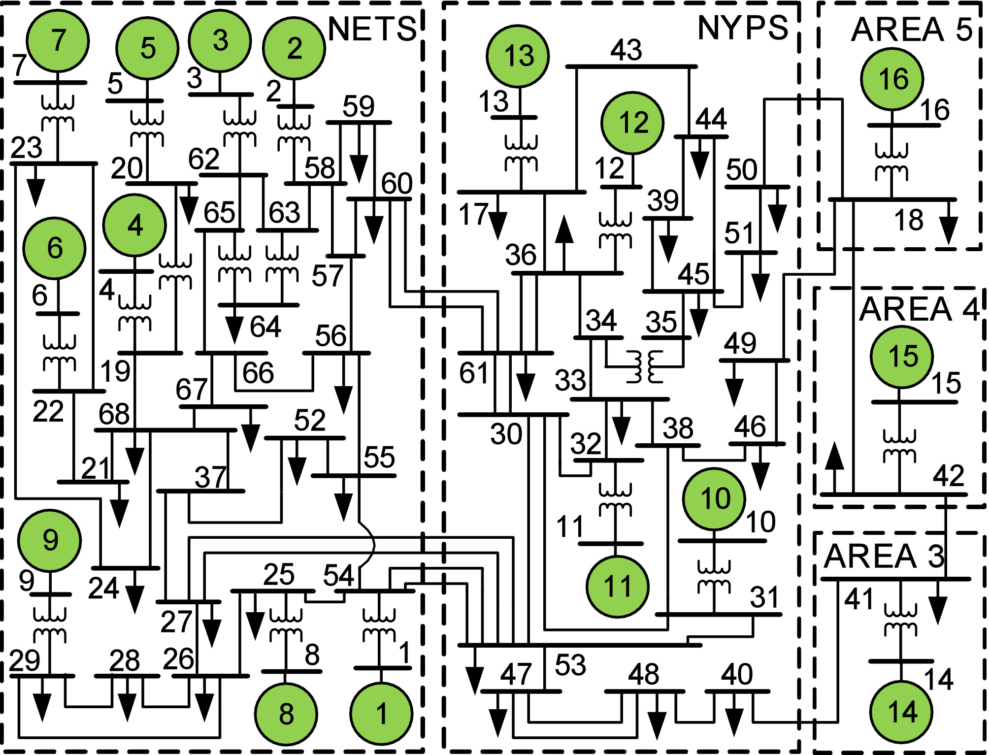
Figure 2: 68-bus, 16-generator, 5-area benchmark system [24].

TABLE I: Wind Power Imbalance With and Without ESS

Bus	$j$	$\mu_{P_{im_{j}}}$ (p.u.)	$\mu_{P_{res_{j}}}$ (p.u.)	Decrease (%)
$19$	$1$	$0.142$	$0.044$	$69.014$
$31$	$2$	$0.138$	$0.046$	$66.667$
$32$	$3$	$0.121$	$0.040$	$66.942$
$62$	$4$	$0.132$	$0.041$	$68.939$

TABLE II: Mean True and Estimated Properties of Inter-Area Mode $3$

ESS	$\operatorname*{\mathbb{E}}(f_{3_{t}})$ (Hz)	$\operatorname*{\mathbb{E}}(f_{3_{e}})$ (Hz)	Err. (%)	$\operatorname*{\mathbb{E}}(\zeta_{3_{t}})$ (%)	$\operatorname*{\mathbb{E}}(\zeta_{3_{e}})$ (%)	Err.(%)
OFF	$0.753$	$0.760$	$0.930$	$1.756$	$1.378$	$21.526$
ON	$0.754$	$0.758$	$0.531$	$1.754$	$1.660$	$5.359$

Note: _t stands for True, _e for Estimated, and Err for Error.

Next, we compute the statistical properties of $A$, $f_{i}$ and $\zeta_{i}$, $i=1,2,3$. To this end, we use $200$ s PMU data with a sampling frequency of $60$ Hz. Simulation results show that wind stochasticity mostly affects the estimation of mode $3$. Therefore, a comparison of the mean true and estimated frequency and damping ratio of inter-area mode $3$ with and without ESS is presented in Table II. Notice that, $\operatorname*{\mathbb{E}}(f_{3})$ is accurately estimated when ESS is OFF despite wind uncertainty. On the other hand, the estimation of $\operatorname*{\mathbb{E}}(\zeta_{3})$ without ESS is poor, thus deteriorating the small-signal stability monitoring. These results demonstrate that the proposed data-driven ESS algorithm can reduce significantly the modal estimation error while requiring only a very small ESS capacity. Similar conclusions can be drawn for the other inter-area modes.

III-B The Algorithm Operation under High Wind Penetration

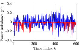
Figure 3: Initial power imbalance ${P_{im_{4}}}(t_{k})$ (displayed in blue) and residual power imbalance ${P_{res_{4}}}(t_{k})$ (displayed in red) for the wind farm of bus $62$.

In this case study, the effectiveness of the proposed ESS algorithm is validated under higher wind power penetration levels. Particularly, we extend the base-case scenario of section III-A by installing additional DFIG-based wind farms of $500$ MW on top of the existing ones in buses $\{19,31,32,62\}$. Thus, three different wind penetration levels are considered:

1. Buses $\{19,32,31,62\}$ – $11\%$ penetration (base case)

2. Buses $\{19,32,31,62,22,58\}$ – $17\%$ penetration

3. Buses $\{19,32,31,62,22,58,35,43\}$ – $23\%$ penetration

while $\{22,58,35,43\}\rightarrow j=\{5,6,7,8\}$, respectively. To visualise the effectiveness of the proposed ESS algorithm, Fig. 3 displays a comparison between the initial power imbalance (ESS is OFF) and the residual power imbalance (ESS is ON) of wind farm at bus $62$ ($j=4$), for a single realization of $\bm{v_{w}}$. With the exception of a few remaining power imbalance spikes, ${P_{res_{4}}}(t_{k})$ becomes zero, thus resulting in an approximately constant wind farm power output. Importantly, $S_{max_{j}}=100$ MW is sufficient to almost eliminate wind power variations despite the penetration increase.

Next, the accuracy of small-signal stability monitoring is assessed. Again, modal analysis is carried out based on $100$ Monte Carlo simulations. Table III summarizes the comparison between the mean absolute percentage error (MAPE) in the estimation of the inter-area mode frequencies ($MAPE_{f}$) and damping ratios ($MAPE_{\zeta}$) when ESS is OFF and the corresponding MAPE when ESS is ON. For illustration purposes, the average of all three modes is computed. As can be seen, frequency errors are trivial irrespective of the ESS application. Nonetheless, damping ratios, which are the main focus of small-signal stability monitoring, exhibit large estimation errors when ESS is deactivated, especially for higher wind penetration levels (e.g. $23\%$). As a result, a poorly-damped inter-area mode can be potentially identified as well-damped. Clearly, our method promotes the accurate estimation of $\zeta_{i}$ by smoothing the unwanted wind power fluctuations.

TABLE III: Mean Absolute Percentage Inter-Area Mode Estimation Error

Wind Penetration	ESS	$MAPE_{f}$ (%)	$MAPE_{\zeta}$ (%)
$11\%$	OFF	$2.316$	$9.609$
	ON	$2.914$	$2.653$
$17\%$	OFF	$1.653$	$9.652$
	ON	$2.214$	$1.659$
$23\%$	OFF	$1.043$	$16.289$
	ON	$1.260$	$3.337$

IV Conclusion and Perspectives

This paper proposed a novel data-driven ESS algorithm for small-signal stability monitoring of power systems with stochastic wind power penetration. Our method can accurately estimate the inter-area mode properties by smoothing the wind power variations, thus enhancing the small-signal stability assessment in near real-time. Numerical simulations demonstrate that the proposed technique achieves the inter-area mode identification and smoothing goals using only a small ESS capacity. Future endeavors will focus on developing methodologies for optimal ESS placement in wind farms and on implementing the proposed data-driven ESS in practice.

References

- [1] S. Bu, W. Du, and H. Wang, \qqInvestigation on probabilistic small-signal stability of power systems as affected by offshore wind generation, IEEE Trans. Power Syst., vol. 30, no. 5, pp. 2479-2486, Sep. 2015.
- [2] S. Bu, W. Du, H. Wang, Z. Chen, L. Xiao, and H. Li, \qqProbabilistic analysis of small-signal stability of large-scale power systems as affected by penetration of wind generation, IEEE Trans. Power Syst., vol. 27, no. 2, pp. 762-770, May 2012.
- [3] G. Andersson et al., \qqCauses of the 2003 major grid blackouts in North America and Europe, and recommended means to improve system dynamic performance, IEEE Trans. Power Syst., vol. 20, no. 4, pp. 1922-1928, Nov. 2005.
- [4] H. Huang, C. Chung, K. Chan, and H. Chen, \qqQuasi-Monte Carlo based probabilistic small signal stability analysis for power systems with plug-in electric vehicle and wind power integration, IEEE Trans. Power Syst., vol. 28, no. 3, pp. 3335-3343, Aug. 2013.
- [5] C. Wang, L. Shi, L. Yao, L. Wang, Y. Ni, and M. Bazargan, \qqModelling analysis in power system small signal stability considering uncertainty of wind generation, in Proc. IEEE PES General Meeting, Providence, RI, 2010.
- [6] F. Daz-González, A. Sumper, O. Gomis-Bellmunt, and R. Villafáfila- Robles, \qqA review of energy storage technologies for wind power applications, Renewable Sust. Energy Rev., vol. 16, no. 4, pp. 2154–2171, May 2012.
- [7] H. Sheng and X. Wang, \qqOnline measurement-based estimation of dynamic system state matrix in ambient conditions, IEEE Trans. Smart Grid, vol. 11, no. 1, pp. 95-105, Jan. 2020.
- [8] I. Zenelis and X. Wang, \qqWide-area damping control for interarea oscillations in power grids based on PMU measurements, IEEE Control Syst. Lett., vol. 2, no. 4, pp. 719-724, Oct. 2018.
- [9] I. Zenelis, X. Wang, and I. Kamwa, \qqOnline PMU-based wide-area damping control for multiple inter-area modes, IEEE Trans. Smart Grid, vol. 11, no. 6, pp. 5451-5461, Nov. 2020.
- [10] Y. Hashmy, Z. Yu, D. Shi, and Y. Weng, \qqWide-area measurement system-based low frequency oscillation damping control through reinforcement learning, IEEE Trans. Smart Grid, vol. 11, no. 6, pp. 5072-5083, Nov. 2020.
- [11] I. Kamwa, R. Grondin, and Y. Hebert, \qqWide-area measurement-based stabilizing control of large power systems–A decentralized/hierarchical approach, IEEE Trans. Power Syst., vol. 16, no. 1, pp. 136-153, Feb. 2001.
- [12] Wide-Area energy storage and management system to balance intermittent resources in the Bonneville Power Administration and California ISO control areas, Pacific Northwest National Laboratory, Tech. Rep., Jun. 2008, [Online]. Available: https://www.osti.gov/biblio/947483
- [13] H. Hasanien, \qqA set-membership affine projection algorithm-based adaptive-controlled SMES units for wind farms output power smoothing, IEEE Trans. Sustain. Energy, vol. 5, no. 4, pp. 1226-1233, Oct. 2014.
- [14] P. Kundur, Power System Stability and Control. New York, NY, USA: McGraw-Hill, 1994.
- [15] T. Odun-Ayo and M. Crow, \qqAn analysis of power system transient stability using stochastic energy functions, Int. Trans. Electr. Energ. Syst., vol. 23, no. 2, pp. 151-165, Oct. 2011.
- [16] J. Carta, P. Ramírez, and S. Velázquez, \qqA review of wind speed probability distributions used in wind energy analysis: Case studies in the Canary Islands, Renewable Sust. Energy Rev., vol. 13, no. 5, pp. 933-955, Jun. 2009.
- [17] F. Milano and R. Zárate-Miñano, \qqA systematic method to model power systems as stochastic differential algebraic equations, IEEE Trans. Power Syst., vol. 28, no. 4, pp. 4537-4544, Nov. 2013.
- [18] X. Wang, H. Chiang, J. Wang, H. Liu, and T. Wang, \qqLong-term stability analysis of power systems with wind power based on stochastic differential equations: model development and foundations, IEEE Trans. Sustain. Energy, vol. 6, no. 4, pp. 1534-1542, Oct. 2015.
- [19] G. Pierrou and X. Wang, \qqThe effect of the uncertainty of load and renewable generation on the dynamic voltage stability margin, in Proc. IEEE PES Innov. Smart Grid Technol. Eur., Bucharest, Romania, 2019.
- [20] J. Slootweg, Wind power: modelling and impact on power system dynamics,, Delft University of Technology, 2003.
- [21] N. Zhou, D. Meng, Z. Huang, and G. Welch, \qqDynamic state estimation of a synchronous machine using pmu data: A comparative study, IEEE Trans. Smart Grid, vol. 6, no. 1, pp. 450-460, Jan. 2015.
- [22] H. Su and A. Gamal, \qqModeling and analysis of the role of energy storage for renewable integration: power balancing, IEEE Trans. Power Syst., vol. 28, no. 4, pp. 4109-4117, Nov. 2013.
- [23] G. Hug, \qqCoordination of intermittent generation with storage, demand control and conventional energy sources. in Proc. IREP Symposium-Bulk Power System Dynamics and Control-VIII, Buzios, Brazil, 2010.
- [24] B. Pal and B. Chaudhuri, Robust Control in Power Systems. New York, NY, USA: Springer, 2005.
- [25] R. Zárate-Miñano, M. Anghel, and F. Milano, \qqContinuous wind speed models based on stochastic differential equations, Appl. Energy, vol. 104, no.1, pp. 42–49, Apr. 2013.
- [26] F. Milano, \qqAn open source power system analysis toolbox, IEEE Trans. Power Syst., vol. 20, no. 3, pp. 1199-1206, Aug. 2005.