Self-Tuning for Data-Efficient Deep Learning

Abstract

Deep learning has made revolutionary advances to diverse applications in the presence of large-scale labeled datasets. However, it is prohibitively time-costly and labor-expensive to collect sufficient labeled data in most realistic scenarios. To mitigate the requirement for labeled data, semi-supervised learning (SSL) focuses on simultaneously exploring both labeled and unlabeled data, while transfer learning (TL) popularizes a favorable practice of fine-tuning a pre-trained model to the target data. A dilemma is thus encountered: Without a decent pre-trained model to provide an implicit regularization, SSL through self-training from scratch will be easily misled by inaccurate pseudo-labels, especially in large-sized label space; Without exploring the intrinsic structure of unlabeled data, TL through fine-tuning from limited labeled data is at risk of under-transfer caused by model shift. To escape from this dilemma, we present Self-Tuning to enable data-efficient deep learning by unifying the exploration of labeled and unlabeled data and the transfer of a pre-trained model, as well as a Pseudo Group Contrast (PGC) mechanism to mitigate the reliance on pseudo-labels and boost the tolerance to false labels. Self-Tuning outperforms its SSL and TL counterparts on five tasks by sharp margins, e.g. it doubles the accuracy of fine-tuning on Cars with $15\%$ labels.

1 Introduction

In the last decade, deep learning has made revolutionary advances to diverse machine learning problems and applications in the presence of large-scale labeled datasets. However, in most real-world scenarios, it is prohibitively time-costly and labor-expensive to collect sufficient labeled data through manual labeling, especially when labeling must be done by an expert such as a doctor in medical applications. To mitigate the requirement for labeled data, semi-supervised learning (SSL) focuses on simultaneously exploring both labeled and unlabeled data, while transfer learning (TL) popularizes a favorable practice of fine-tuning a pre-trained model to the target data.

Semi-supervised learning (SSL) is a powerful approach for addressing the lack of labeled data by also exploring unlabeled examples. Recent advances in semi-supervised learning (Sohn et al., 2020; Chen et al., 2020b) reveal that self-training (Lee, 2013), which picks up the class with the highest predicted probability of a sample as its pseudo-label, is empirically and theoretically (Wei et al., 2021) proved effective on unlabeled data. However, an obvious obstacle in pseudo-labeling is the confirmation bias (Arazo et al., 2020): the performance of a student is restricted by the teacher when learning from inaccurate pseudo-labels. In a prior study, we investigated the current state-of-the-art SSL method, FixMatch (Sohn et al., 2020), on a target dataset CUB-200-2011 (Wah et al., 2011) containing $200$ bird species. As Figure 4(a) shows, keeping the same label proportion of 15%, the test accuracy of FixMatch drops rapidly as the descending accuracy of pseudo-labels when the label space enlarges from $10$ (CUB10) to $200$ (CUB200). This observation reveals that SSL through self-training from scratch, without a decent pre-trained model to provide an implicit regularization, will be easily misled by inaccurate pseudo-labels, especially in large-sized label space.

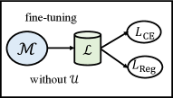
(a) Transfer Learning

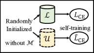
(b) Semi-supervised Learning

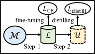
(c) SimCLRv2

(d) Self-Tuning (ours)

Figure 1: Comparisons among techniques. (a) Transfer Learning: only fine-tuning on $\mathcal{L}$ with a regularization term; (b) Semi-supervised Learning: a common practice for SSL is a CE loss on $\mathcal{L}$ while self-training on $\mathcal{U}$ without a decent pretrained model; (c) SimCLRv2: fine-tune model $\mathcal{M}$ on $\mathcal{L}$ first and then distill on $\mathcal{U}$; (d) Self-Tuning: unify the exploration of $\mathcal{L}$ and $\mathcal{U}$ and the transfer of model $\mathcal{M}$.

Fine-tuning a pre-trained model to a labeled target dataset is a popular form of transfer learning (TL) and increasingly becoming a common practice within computer vision (CV) and natural language processing (NLP) communities. For instance, ResNet (He et al., 2016) and EfficientNet (Tan & Le, 2019) models pre-trained on ImageNet (Deng et al., 2009) are widely fine-tuned into various CV tasks, while BERT (Devlin et al., 2018) and GPT-3 (Brown et al., 2020) models pre-trained on large-scale corpus achieve strong performance on diverse NLP tasks. Recent works on fine-tuning mainly focus on how to better exploit a target labeled data and a pre-trained model from various perspectives, such as weights (Li et al., 2018), features (Li et al., 2019), singular values (Chen et al., 2019) and category relationship (You et al., 2020). In a prior study, we investigated the current state-of-the-art TL method, Co-Tuning, on standard TL benchmarks: CUB-200-2011 and Stanford Cars (Krause et al., 2013). As shown in Figure 4(b), the test accuracy of Co-Tuning declines rapidly as the number of labeled data decreases. This observation tells us: without exploring the intrinsic structure of unlabeled data, TL through fine-tuning from limited labeled data is at risk of under-transfer caused by model shift: the fine-tuned model shifts towards the limited labeled data and leaves away from the original smooth model pre-trained on a large-scale dataset, causing an unsatisfactory performance on the test set.

Realizing the drawback of only developing TL or SSL technique, a recent state-of-the-art paper named SimCLRv2 (Chen et al., 2020b) provided a new and interesting solution by fine-tuning from a big ImageNet pre-trained model $\mathcal{M}$ on a labeled data $\mathcal{L}$ first and then distilling on the unlabeled data $\mathcal{U}$. Its effectiveness has been demonstrated when fine-tuning to the same ImageNet dataset. However, we empirically found its unsatisfactory performance when transferring to cross-domain datasets, especially in the low-data regime, as reported in Table 4.2. We hypothesize that the sequential form between first fine-tuning on $\mathcal{L}$ and then distilling on $\mathcal{U}$ that SimCLRv2 adopts is to blame, since the fine-tuned model would easily shift towards the limited labeled data with sampling bias and leaves away from the original smooth model pre-trained on a large-scale dataset.

To escape from the dilemma, we present Self-Tuning, a novel approach to enable data-efficient deep learning. Specifically, to address the challenge of confirmation bias in self-training, a Pseudo Group Contrast (PGC) mechanism is devised to mitigate the reliance on pseudo-labels and boost the tolerance to false labels, after realizing the drawbacks of cross-entropy (CE) loss and contrastive learning (CL) loss. The model trained by CE loss will be easily confused by false pseudo-labels since it focuses on learning a hyperplane for discriminating each class from the other classes, while standard CL loss lacks a mechanism to tailor pseudo-labels into model training, leaving the useful discriminative information on the shelf. Further, we propose to unify the exploration of labeled and unlabeled data and the transfer of a pre-trained model to tackle the model shift problem, different from the sequential form of exploring labeled and unlabeled data. Comparisons among these techniques are shown in Figure 1, revealing the advantages of Self-Tuning.

In summary, this paper has the following contributions:

• Realizing the dilemma of TL and SSL methods that only focus on either the pre-trained model or unlabeled data, we unleash the power of both worlds by proposing a new setup named data-efficient deep learning.

• To tackle model shift and confirmation bias problems, we propose Self-Tuning to unify the exploration of labeled and unlabeled data and the transfer of a pre-trained model, as well as a general Pseudo Group Contrast mechanism to mitigate the reliance on pseudo-labels and boost the tolerance to false labels.

• Comprehensive experiments demonstrate that Self-Tuning outperforms its SSL and TL counterparts on five tasks by sharp margins, e.g. it doubles the accuracy of fine-tuning on Cars with $15\%$ labels.

2 Related Work

2.1 Self-training in Semi-supervised Learning

Self-training (Yarowsky, 1995; Grandvalet & Bengio, 2004; Lee, 2013) is a widely-used technique for exploring unlabeled data with deep neural networks, especially in SSL. Among techniques of self-training, pseudo-labeling (Lee, 2013) is one of the most popular forms by leveraging the model itself to obtain artificial labels for unlabeled data. Recent advances in SSL reveal that self-training is empirically (Sohn et al., 2020) and theoretically (Wei et al., 2021) effective on unlabeled data. These methods either require stability of predictions under different data augmentations (Tarvainen & Valpola, 2017; Xie et al., 2020; Sohn et al., 2020) (also known as input consistency regularization) or fit the unlabeled data on its predictions generated by a previously learned model (Lee, 2013; Chen et al., 2020b). Specifically, UDA (Xie et al., 2020) reveals that the quality of noising produced by advanced data augmentation methods plays a crucial role in SSL. FixMatch (Sohn et al., 2020) uses the model’s predictions on weakly-augmented unlabeled images to generate pseudo-labels for the strongly-augmented versions of the same images. A recent state-of-the-art paper named SimCLRv2 (Chen et al., 2020b) provided a new solution for SSL by first fine-tuning from the labeled data and then distilling on the unlabeled data.

However, without a decent pre-trained model to provide an implicit regularization, SSL through self-training from scratch will be easily misled by inaccurate pseudo-labels, especially in large-sized label space. Meanwhile, an obvious obstacle in pseudo-labeling is confirmation bias (Arazo et al., 2020): the performance of a student is restricted by the teacher when learning from inaccurate pseudo-labels.

2.2 Fine-tuning in Transfer Learning

Fine-tuning a pre-trained model to a labeled target dataset is a popular form of transfer learning (TL) and widely applied in various applications. Previously, Donahue et al. (2014); Oquab et al. (2014) show that transferring features extracted by pre-trained AlexNet model to downstream tasks provides better performance than that of hand-crafted features. Later, Yosinski et al. (2014); Agrawal et al. (2014); Girshick et al. (2014) reveal that fine-tuning pre-trained networks work better than fixed pre-trained representations. Recent works on fine-tuning mainly focus on how to better exploit the discriminative knowledge of labeled data and the information of pre-trained models from different perspectives. (a) weights: L2-SP (Li et al., 2018) explicitly promotes the similarity of the final solution with pre-trained weights by a simple L2 penalty. (b) features: DELTA (Li et al., 2019) constrains a subset of feature maps with the pre-trained activations that are precisely selected by channel-wise attention. (c) singular values: BSS (Chen et al., 2019) penalizes smaller singular values to suppress untransferable spectral components to avoid negative transfer. (d) category relationship: Co-Tuning (You et al., 2020) learns the relationship between source categories and target categories from the pre-trained model to enable a full transfer. Even when the target dataset is very dissimilar to the pre-trained dataset and fine-tuning brings no performance gain (Raghu et al., 2019), it can accelerate the convergence speed (He et al., 2019). Meanwhile, NLP research on fine-tuning has an alternative focus on resource consumption (Houlsby et al., 2019; Garg et al., 2020), selective layer freezing (Wang et al., 2019), different learning rates (Sun et al., 2019) and scaling up language models (Brown et al., 2020).

However, without exploring the intrinsic structure of unlabeled data, TL through fine-tuning from limited labeled data is at risk of under-transfer caused by model shift: the fine-tuned model shifts towards the limited labeled data after leaving away from the original smooth model pre-trained on a large-scale dataset, causing an unsatisfactory test accuracy on the target dataset that we concern.

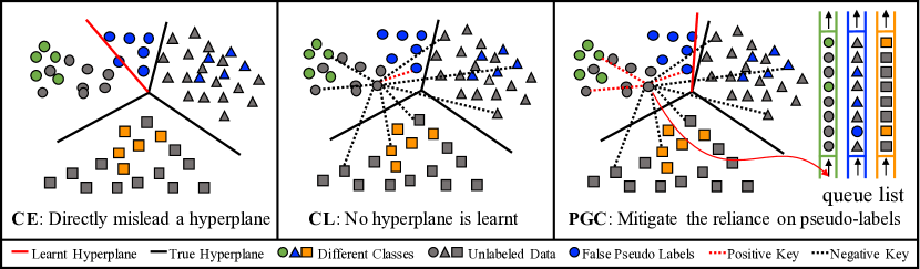
Figure 2: Comparison of various loss functions: (a) CE: cross-entropy loss will be easily misled by false pseudo-labels; (b) CL: contrastive learning loss underutilizes labels and pseudo-labels; (c) PGC: Pseudo Group Contrast mechanism to mitigate confirmation bias.

3 Preliminaries

3.1 The Devil Lies in Cross-Entropy Loss

To figure out the confirmation bias of pseudo-labeling, we first delve into the standard cross-entropy (CE) loss that most self-training methods adopt. Given labeled data $\mathcal{L}$ with $C$ categories, $y_{i}$ is the ground-truth label for each data point $\mathbf{x}_{i}$ whose prediction probability $\mathbf{p}_{i}=\mathcal{M}(\mathbf{x}_{i})$ is generated from model $\mathcal{M}$. For each data point $\mathbf{x}_{i}$, the standard CE loss can be formalized as

$$L_{\rm CE}=-\sum_{c=1}^{C}\mathbf{1}({y}_{i}=c)\log\mathbf{p}_{i}^{c},$$ (1)

where $\mathbf{1}(\cdot)\in\{0,1\}$ is an indicator function that values $1$ if and only if the input condition holds. Similarly, for each data point $\mathbf{x}_{i}$ with prediction probability $\mathbf{p}_{i}=\mathcal{M}(\mathbf{x}_{i})$, self-training loss on unlabeled data $\mathcal{U}$ is

$$\widehat{L}_{\rm CE}=-\sum_{c=1}^{C}\mathbf{1}(\widehat{y}_{i}=c)\mathbf{1}(z_{i}>t)\log\mathbf{p}_{i}^{c},$$ (2)

where $\widehat{y}_{i}=\operatorname*{arg\,max}_{c}\mathbf{p}_{i}^{c}$ is the pseudo-label for the input $\mathbf{x}_{i}$ generated by a previously-learned model or from the input with different data augmentation, $z_{i}=\max_{c}(\mathbf{p}_{i}^{c})$ is the corresponding confidence, and $t$ is the threshold to select out more confident pseudo-labels. Note that the confidence-threshold $t$ is necessary in most self-training methods and set with a high value, e.g. $t=0.95$ in FixMatch, or even with a complicated curriculum strategy. Such a self-training loss is effective in exploring unlabeled data. However, as shown in Figure 2, the model trained by CE loss will be easily confused by false pseudo-labels since it focuses on learning a hyperplane for discriminating each class from the other classes, causing the unsatisfactory performance on target dataset with large-sized label space.

3.2 Contrastive Learning Loss Underutilizes Labels

To overcome the drawbacks of class discrimination for self-training, recent advanced researches of instance discrimination (van den Oord et al., 2018; Wu et al., 2018; He et al., 2020; Chen et al., 2020a) attract our great attention. Given an encoded query $\mathbf{q}$ and encoded keys $\{{\mathbf{k}_{0}},\mathbf{k}_{1},\mathbf{k}_{2},\cdots,\mathbf{k}_{D}\}$ with size $(D+1)$, a general form of contrastive learning (CL) loss with similarity measured by dot product for each data point on unlabeled data $\mathcal{U}$ is

$$L_{\rm{CL}}=-\log\frac{\exp(\mathbf{q}\cdot\mathbf{k}_{0}/\tau)}{\exp(\mathbf{q}\cdot\mathbf{k}_{0}/\tau)+\sum_{d=1}^{D}\exp(\mathbf{q}\cdot\mathbf{k}_{d}/\tau)},$$ (3)

where $\tau$ is a hyper-parameter for temperature scaling. Note that $\mathbf{k}_{0}$ is the only positive key that $\mathbf{q}$ matches since they are extracted from differently augmented views of the same data example, while negative keys $\{\mathbf{k}_{1},\mathbf{k}_{2},\cdots,\mathbf{k}_{D}\}$ are selected from a dynamic queue which iteratively and progressively replace the oldest samples by the newly-generated keys. A contrastive loss maximizes the similarity between the query $\mathbf{q}$ with its corresponding positive key $\mathbf{k}_{0}$. According to the properties of the softmax function adopted in Eq. (3), the similarity between the query with those negative keys $\{\mathbf{k}_{1},\mathbf{k}_{2},\cdots,\mathbf{k}_{D}\}$ is minimized. Maximizing agreement between differently augmented views of the same data point, CL loss focuses on exploring the intrinsic structure of data and is naturally independent of false pseudo-labels. However, standard CL loss lacks a mechanism to tailor labels and pseudo-labels into model training, leaving the useful discriminative information on the shelf.

4 Self-Tuning

In data-efficient deep learning, a pre-trained model $\mathcal{M}$, a labeled dataset $\mathcal{L}=\left\{\left(\mathbf{x}_{i}^{L},{y}_{i}^{L}\right)\right\}_{i=1}^{n_{L}}$ and an unlabeled dataset $\mathcal{U}=\left\{\left(\mathbf{x}_{i}^{U}\right)\right\}_{i=1}^{n_{U}}$ in the target domain are given. Instantiated as a deep network, $\mathcal{M}$ is composed of a pre-trained backbone $f_{0}$ for feature extraction and a pre-trained head $g_{0}$, while fine-tuned ones are denoted by $f$ and $g$ respectively. $f$ is usually initialized as $f_{0}$ while $g$ is randomly initialized, since the target dataset usually has a different label space with size $C$ from that of pre-trained models. There are two obstables in such a practical paradigm: confirmation bias and model shift, which are addressed by pseudo group contrast mechanism and unifying the exploration respectively.

4.1 Confirmation Bias: Pseudo Group Contrast

As mentioned in Preliminaries 3, neither cross-entropy loss nor contrastive learning loss is a suitable loss function to address the challenge of confirmation bias in self-training. In this paper, a novel Pseudo Group Contrast (PGC) mechanism is raised to mitigate the reliance on pseudo-labels and boost the tolerance to false labels. Different from the standard CL which involves just a positive key in each contrast, PGC introduces a group of positive keys in the same pseudo-class to contrast with all negative keys from other pseudo-classes. Specifically, for each data point $\mathbf{x}_{i}^{U}$ in unlabeled dataset $\mathcal{U}$, an encoded query $\mathbf{q}_{i}^{U}=h(f({\rm aug}_{1}(\mathbf{x}_{i}^{U})))$ and an encoded key $\mathbf{k}_{i}^{U}=h(f({\rm aug}_{2}(\mathbf{x}_{i}^{U})))$ are generated by a feature extractor $f$ following with a projector head $h$ on two differently-augmented views ${\rm aug}_{1}$ and ${\rm aug}_{2}$ of the same data example. By forwarding into the classifier $g$, a pseudo-label $\widehat{y}_{i}^{U}=\operatorname*{arg\,max}_{c}g(f({\rm aug}_{1}(\mathbf{x}_{i}^{U})))$ is attained.

For clarity, we focus on a particular data example $\mathbf{x}$ with pseudo-label $\widehat{y}$ and omit the subscript $i$ and the superscript $U$. Different from standard CL loss, a group of positive keys $\{\mathbf{k}_{1}^{\widehat{y}},\mathbf{k}_{2}^{\widehat{y}},\cdots,\mathbf{k}_{D}^{\widehat{y}}\}$ are selected according to its pseudo-label $\widehat{y}$, as well as its ${\mathbf{k}_{0}^{\widehat{y}}}$ generated by its differently-augmented view. In this way, the scope of positive keys is successfully expanded from a single one to a group of instances with size $D+1$. Complementarily, all keys from other pseudo-classes are seen as negative keys with size $[D\times(C-1)]$, selected from the dynamic queue list with size $[D\times C]$ according to their pseudo-labels. Note that, $D$ in PGC is equal to the queue size in standard CL divided by $C$, resulting in a comparable memory consumption. Formally, for each data point $\mathbf{x}_{i}^{U}$ on unlabeled data $\mathcal{U}$, PGC loss is summarized as

$$\widehat{L}_{\text{PGC}} =-\frac{1}{D+1}\sum_{d=0}^{D}\log\frac{\exp(\mathbf{q}\cdot\mathbf{k}_{d}^{\widehat{y}}/\tau)}{\rm Pos+\rm Neg}$$ (4)

$${\rm Pos} =\exp(\mathbf{q}\cdot\mathbf{k}_{0}^{\widehat{y}}/\tau)+\sum_{j=1}^{D}\exp(\mathbf{q}\cdot\mathbf{k}_{j}^{\widehat{y}}/\tau)$$

$${\rm Neg} =\sum_{c=1}^{\{1,2,\cdots,C\}\backslash\widehat{y}}\sum_{j=1}^{D}\exp(\mathbf{q}\cdot\mathbf{k}_{j}^{c}/\tau),$$

where the term of $\rm Pos$ denotes positve keys from the same pseudo-class $\widehat{y}$ while the term of $\rm Neg$ denotes negative keys from other pseudo-classes $\{1,2,\cdots,C\}\backslash\widehat{y}$. Obviously, PGC maximizes the similarity between the query $\mathbf{q}$ with its corresponding group of positive keys $\{{\mathbf{k}_{0}^{\widehat{y}}},\mathbf{k}_{1}^{\widehat{y}},\mathbf{k}_{2}^{\widehat{y}},\cdots,\mathbf{k}_{D}^{\widehat{y}}\}$ from the same pseudo-class $\widehat{y}$.

Further, according to the property of the softmax function which generates a predicted probability vector with a sum of $1$, positive keys $\{{\mathbf{k}_{0}^{\widehat{y}}},\mathbf{k}_{1}^{\widehat{y}},\mathbf{k}_{2}^{\widehat{y}},\cdots,\mathbf{k}_{D}^{\widehat{y}}\}$ from the same pseudo-class will compete with each other. Therefore, if some pseudo-labels in the positive group are wrong, those keys with true pseudo-labels will win this instance competition, since their representations are more similar to the query, compared to that of false ones. Consequently, the model trained by PGC will be mainly updated by gradients of true pseudo-labels and largely avoid being misled by false pseudo-labels. Since PGC itself can mitigate the reliance on pseudo-labels and boost the tolerance to false labels, no confidence-threshold hyper-parameter $t$ is included in PGC, making it easier to apply into new datasets than standard self-training in Eq.(2). A conceptual comparison between PGC with CE and CL is shown in Figure 2. Ablation studies in Table 5 also confirm that PGC performs much better than CE and CL when initializing from an identical pre-trained model with the same pseudo-label accuracy.

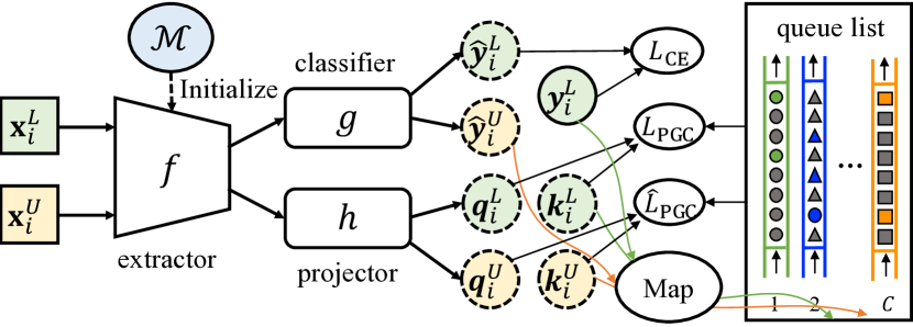
Figure 3: The network architecture of Self-Tuning. The “Map” denotes a mapping function which assigns a newly-generated key to the corresoping queue according to its label or pseudo-label.

4.2 Model Shift: Unifying and Sharing

Recall the model shift problem of transfer learning through fine-tuning from limited labeled data: the fine-tuned model shifts towards the limited labeled data after leaving away from the original smooth model pre-trained on a large-scale dataset, causing an unsatisfactory performance on the test set. A recent state-of-the-art paper named SimCLRv2 (Chen et al., 2020b) gives an interesting solution of fine-tuning from a big pre-trained model $\mathcal{M}$ on a labeled data $\mathcal{L}$ first and then distilling on the unlabeled data $\mathcal{U}$. However, due to the sequential form it adopts, the fine-tuned model still easily shifts towards the limited labeled data with sampling bias and leaves away from the original smooth model. To this end, we propose to unify the exploration of labeled and unlabeled data and the transfer of a pre-trained model.

A unified form to fully exploit $\mathcal{M}$, $\mathcal{L}$ and $\mathcal{U}$

Realizing the drawbacks of the sequential form of first fine-tuning on the labeled data and then distilling on the unlabeled data, we propose a unified form to fully exploit $\mathcal{M}$, $\mathcal{L}$ and $\mathcal{U}$ to tackle the model shift problem. First, initialized from a decently accurate pre-trained model, Self-Tuning has a better starting point to provide an implicit regularization than the model trained from scratch on the target dataset.

Further, the knowledge of the pre-trained model parallelly flows into both the labeled and unlabeled data, which is different from the sequential form that overfits the limited labeled data first. Meanwhile, the parameters of the model will be simultaneously updated by gradients from both the labeled data $\mathcal{L}$ and unlabeled data $\mathcal{U}$. By exploring the label information of $\mathcal{L}$ and intrinsic structure of $\mathcal{U}$ at the same time in a unified form as shown in Figure 1(d), the model shift challenge is expected to be alleviated.

A shared queue list across $\mathcal{L}$ and $\mathcal{U}$

Given a labeled data $\mathcal{L}=\left\{\left(\mathbf{x}_{i}^{L},{y}_{i}^{L}\right)\right\}_{i=1}^{n_{L}}$ from $C$ categories, its ground-truth labels are readily-available. For a data sample $\left(\mathbf{x}_{i}^{L},{y}_{i}^{L}\right)$ in $\mathcal{L}$, its encoded query $\mathbf{q}_{i}^{L}=h(f({\rm aug}_{1}(\mathbf{x}_{i}^{L})))$ and encoded key $\mathbf{k}_{i}^{L}=h(f({\rm aug}_{2}(\mathbf{x}_{i}^{L})))$ are generated similarly. For clarity, we focus on a particular data example $\left(\mathbf{x},{y}\right)$ and omit the subscript $i$ and the superscript $L$. Intuitively, we can simply replace the $\widehat{y}$ in Eq. (4) with ${y}$ to attain the ground-truth version of PGC on the labeled data. Formally, for each data point $\left(\mathbf{x},{y}\right)$ on $\mathcal{L}$, PGC loss is summarized as

$$L_{\text{PGC}} =-\frac{1}{D+1}\sum_{d=0}^{D}\log\frac{\exp(\mathbf{q}\cdot\mathbf{k}_{d}^{{y}}/\tau)}{\rm Pos+\rm Neg},$$ (5)

where the term of $\rm Pos$ and $\rm Neg$ are simlarly defined as that in Eq. (4) except replacing $\widehat{y}$ with ${y}$.

It is noteworthy that the queue list is shared across labeled and unlabeled data, that is, encoded keys generated from both $\mathcal{L}$ and $\mathcal{U}$ will iteratively and progressively replace the oldest samples in the same queue list according to their labels or pseudo-babels. This design tailors ground-truth labels from the labeled data into the shared queue list, thus improving the accuracy of candidate keys for unlabeled queries $\mathbf{q}_{i}^{U}$ than that of a separate queue for unlabeled data.

Besides $L_{\text{PGC}}$ and $\widehat{L}_{\text{PGC}}$, a standard cross-entropy (CE) loss on labeled data is applied on the prediction probability $\mathbf{p}_{i}=g(f(\mathbf{x}_{i}^{L}))$ for each data point $\mathbf{x}_{i}^{L}$ as Eq. (1). The overall loss function of Self-Tuning can be formulated as follows:

$$\mathbb{E}_{\left(\mathbf{x}_{i},{y}_{i}\right)\in\mathcal{L}}\left(L_{\rm CE}+L_{\rm PGC}\right)+\mathbb{E}_{(\mathbf{x}_{i})\in\mathcal{U}}\widehat{L}_{\rm PGC}.$$

It is worthy to mention that no trade-off coefficients between the above losses are introduced since the magnitude of these loss terms is comparable. In summary, the network architecture of Self-Tuning is illustrated in Figure 3.

Table 1: Classification accuracy (%) $\uparrow$ of Self-Tuning and various baselines on standard TL benchmarks (ResNet-50 pre-trained).

Dataset	Type	Method	Label Proportion
			$15\%$	$30\%$	$50\%$	$100\%$
CUB-200-2011	TL	Fine-Tuning (baseline)	45.25$\pm$0.12	59.68$\pm$0.21	70.12$\pm$0.29	78.01$\pm$0.16
		$\rm{L^{2}}$-$\rm{SP}$ (Li et al., 2018)	45.08$\pm$0.19	57.78$\pm$0.24	69.47$\pm$0.29	78.44$\pm$0.17
		$\rm{DELTA}$ (Li et al., 2019)	46.83$\pm$0.21	60.37$\pm$0.25	71.38$\pm$0.20	78.63$\pm$0.18
		$\rm{BSS}$ (Chen et al., 2019)	47.74$\pm$0.23	63.38$\pm$0.29	72.56$\pm$0.17	78.85$\pm$0.31
		Co-Tuning (You et al., 2020)	52.58$\pm$0.53	66.47$\pm$0.17	74.64$\pm$0.36	81.24$\pm$0.14
	SSL	$\Pi$-model (Laine & Aila, 2017)	45.20$\pm$0.23	56.20$\pm$0.29	64.07$\pm$0.32	–
		Pseudo-Labeling (Lee, 2013)	45.33$\pm$0.24	62.02$\pm$0.31	72.30$\pm$0.29	–
		Mean Teacher (Tarvainen & Valpola, 2017)	53.26$\pm$0.19	66.66$\pm$0.20	74.37$\pm$0.30	–
		UDA (Xie et al., 2020)	46.90$\pm$0.31	61.16$\pm$0.35	71.86$\pm$0.43	–
		FixMatch (Sohn et al., 2020)	44.06$\pm$0.23	63.54$\pm$0.18	75.96$\pm$0.29	–
		SimCLRv2  (Chen et al., 2020b)	45.74$\pm$0.15	62.70$\pm$0.24	71.01$\pm$0.34	–
	Combine	Co-Tuning + Pseudo-Labeling	54.11$\pm$0.24	68.07$\pm$0.32	75.94$\pm$0.34	–
		Co-Tuning + Mean Teacher	57.92$\pm$0.18	67.98$\pm$0.25	72.82$\pm$0.29	–
		Co-Tuning + FixMatch	46.81$\pm$0.21	58.88$\pm$0.23	73.07$\pm$0.29	–
		Self-Tuning (ours)	64.17$\pm$0.47	75.13$\pm$0.35	80.22$\pm$0.36	83.95$\pm$0.18
Stanford Cars	TL	Fine-Tuning (baseline)	36.77$\pm$0.12	60.63$\pm$0.18	75.10$\pm$0.21	87.20$\pm$0.19
		$\rm{L^{2}}$-$\rm{SP}$ (Li et al., 2018)	36.10$\pm$0.30	60.30$\pm$0.28	75.48$\pm$0.22	86.58$\pm$0.26
		$\rm{DELTA}$ (Li et al., 2019)	39.37$\pm$0.34	63.28$\pm$0.27	76.53$\pm$0.24	86.32$\pm$0.20
		$\rm{BSS}$ (Chen et al., 2019)	40.57$\pm$0.12	64.13$\pm$0.18	76.78$\pm$0.21	87.63$\pm$0.27
		Co-Tuning (You et al., 2020)	46.02$\pm$0.18	69.09$\pm$0.10	80.66$\pm$0.25	89.53$\pm$0.09
	SSL	$\Pi$-model (Laine & Aila, 2017)	45.19$\pm$0.21	57.29$\pm$0.26	64.18$\pm$0.29	–
		Pseudo-Labeling (Lee, 2013)	40.93$\pm$0.23	67.02$\pm$0.19	78.71$\pm$0.30	–
		Mean Teacher (Tarvainen & Valpola, 2017)	54.28$\pm$0.14	66.02$\pm$0.21	74.24$\pm$0.23	–
		UDA (Xie et al., 2020)	39.90$\pm$0.43	64.16$\pm$0.40	71.86$\pm$0.56	–
		FixMatch (Sohn et al., 2020)	49.86$\pm$0.27	77.54$\pm$0.29	84.78$\pm$0.33	–
		SimCLRv2  (Chen et al., 2020b)	45.74$\pm$0.16	61.70$\pm$0.18	77.49$\pm$0.24	–
	Combine	Co-Tuning + Pseudo-Labeling	50.16$\pm$0.23	73.76$\pm$0.26	83.33$\pm$0.34	–
		Co-Tuning + Mean Teacher	52.98$\pm$0.19	71.42$\pm$0.24	75.38$\pm$0.29	–
		Co-Tuning + FixMatch	42.34$\pm$0.19	73.24$\pm$0.25	83.13$\pm$0.34	–
		Self-Tuning (ours)	72.50$\pm$0.45	83.58$\pm$0.28	88.11$\pm$0.29	90.67$\pm$0.23
FGVC Aircraft	TL	Fine-tuning (baseline)	39.57$\pm$0.20	57.46$\pm$0.12	67.93$\pm$0.28	81.13$\pm$0.21
		$\rm{L^{2}}$-$\rm{SP}$ (Li et al., 2018)	39.27$\pm$0.24	57.12$\pm$0.27	67.46$\pm$0.26	80.98$\pm$0.29
		DELTA (Li et al., 2019)	42.16$\pm$0.21	58.60$\pm$0.29	68.51$\pm$0.25	80.44$\pm$0.20
		BSS (Chen et al., 2019)	40.41$\pm$0.12	59.23$\pm$0.31	69.19$\pm$0.13	81.48$\pm$0.18
		Co-Tuning (You et al., 2020)	44.09$\pm$0.67	61.65$\pm$0.32	72.73$\pm$0.08	83.87$\pm$0.09
	SSL	$\Pi$-model (Laine & Aila, 2017)	37.32$\pm$0.25	58.49$\pm$0.26	65.63$\pm$0.36	–
		Pseudo-Labeling (Lee, 2013)	46.83$\pm$0.30	62.77$\pm$0.31	73.21$\pm$0.39	–
		Mean Teacher (Tarvainen & Valpola, 2017)	51.59$\pm$0.23	71.62$\pm$0.29	80.31$\pm$0.32	–
		UDA (Xie et al., 2020)	43.96$\pm$0.45	64.17$\pm$0.49	67.42$\pm$0.53	–
		FixMatch (Sohn et al., 2020)	55.53$\pm$0.26	71.35$\pm$0.35	78.34$\pm$0.43	–
		SimCLRv2  (Chen et al., 2020b)	40.78$\pm$0.21	59.03$\pm$0.29	68.54$\pm$0.30	–
	Combine	Co-Tuning + Pseudo-Labeling	49.15$\pm$0.32	65.62$\pm$0.34	74.57$\pm$0.40	–
		Co-Tuning + Mean Teacher	51.46$\pm$0.25	64.30$\pm$0.28	70.85$\pm$0.35	–
		Co-Tuning + FixMatch	53.74$\pm$0.23	69.91$\pm$0.26	80.02$\pm$0.32	–
		Self-Tuning (ours)	64.11$\pm$0.32	76.03$\pm$0.25	81.22$\pm$0.29	84.28$\pm$0.14

5 Experiments

We empirically evaluate Self-Tuning in several dimensions: (1) Task Variety: four visual tasks with various dataset scales including CUB-200-2011 (Wah et al., 2011), Stanford Cars (Krause et al., 2013) and FGVC Aircraft (Maji et al., 2013) and CIFAR-100 (Krizhevsky & Hinton, 2009) , as well as one NLP task: CoNLL 2013 (Sang & Meulder, 2003). (2) Label Proportion: the proportion of labeled dataset ranging from $15\%$ to $50\%$ following the common practice of transfer learning, as well as including $4$ labels and $25$ labels per class following the popular protocol of semi-supervised learning. (3) Pre-trained models: mainstream pre-trained models are adopted including ResNet-18, ResNet-50 (He et al., 2016), EfficientNet (Tan & Le, 2019), MoCov2 (He et al., 2020) and BERT (Devlin et al., 2018).

Baselines

We compared Self-Tuning against three types of baselines: (1) Transfer Learning (TL): besides the vanilla fine-tuning, four state-of-the-art TL techniques: L2SP (Li et al., 2018), DELTA (Li et al., 2019), BSS (Chen et al., 2019) and Co-Tuning (You et al., 2020) are included. (2) Semi-supervised Learning (SSL): we include three classical SSL methods: $\Pi$-model (Laine & Aila, 2017), Pseudo-Labeling (Lee, 2013), and Mean Teacher (Tarvainen & Valpola, 2017), as well as three state-of-the-art SSL methods: UDA (Xie et al., 2020), FixMatch (Sohn et al., 2020), and SimCLRv2 (Chen et al., 2020b). Note that all SSL methods are initialized from a ResNet-50 pre-trained model for a fair comparison with TL methods. (3) TL + SSL: Strong combinations TL and SSL methods are included as our baselines, including Co-Tuning + FixMatch, Co-Tuning + Pseudo-Labeling, Co-Tuning + Mean Teacher. FixMatch, UDA, and Self-Tuning use the same RandAugment method, while other baselines use normal ones.

Implementation Details

For a given pre-trained model, we replace its last-layer with a randomly initialized task-specific layer as the classifier $g$ whose learning rate is $10$ times that for pre-trained parameters, following the common fine-tuning principle (Yosinski et al., 2014). Meanwhile, another randomly initialized projector head $h$ is introduced to generate the representations of the query or key. Following MoCo (He et al., 2020), we adopted a default temperature $\tau=0.07$, a learning rate ${\rm lr}=0.001$ and a queue size $D=32$ for each category. SGD with a momentum of $0.9$ is adopted as the optimizer. Each experiment is repeated three times with different random seeds. Code will be available at github.com/thuml/Self-Tuning.

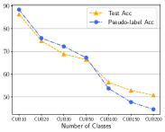
(a) Acc of FixMatch on CUB

(b) Test accuracy of Co-Tuning

Figure 4: Test accuracy of a state-of-the-art SSL method and a TL method on various class numbers or label ratios respectively.

5.1 A Prior Study

In a prior study, we investigated the current state-of-the-art SSL method, FixMatch (Sohn et al., 2020), on a target dataset CUB-200-2011 (Wah et al., 2011) containing $200$ bird species. As Figure 4(a) shows, keeping a same label proportion of 15%, the test accuracy of FixMatch drops rapidly as the descending accuracy of pseudo-labels when the label space enlarges from $10$ (CUB10) to $200$ (CUB200). We further investigated the current state-of-the-art TL method, Co-Tuning, on standard TL benchmarks: CUB-200-2011 and Stanford Cars (Krause et al., 2013). As shown in Figure 4(b), the test accuracy of Co-Tuning declines rapidly as the number of labeled data decreases.

5.2 Standard Transfer Learning Benchmarks

The standard TL benchmarks extensively investigated in previous fine-tuning techniques (You et al., 2020) consist of CUB-200-2011 ($11,788$ images for $200$ bird species), Stanford Cars ($16,185$ images for $196$ car categories), and FGVC Aircraft ($10,000$ images for $100$ aircraft variants). Co-Tuning has two steps, in which the first step of calculating the category relationship relies on the certainty of data augmentation. From Pseudo-Labeling to FixMatch, the randomness of data augmentation increases. Therefore, Pseudo-Labeling benefits from adding Co-Tuning while FixMatch does not, as reported in Table 4.2. Further, these results show that neither a simple combination of SSL and TL methods nor a sequential form between labeled and unlabeled data proposed by a prior work called SimCLRv2 achieve satisfactory performance on the target dataset.

Contrarily, by unifying the exploration of labeled and unlabeled data and the transfer of a pre-trained model, Self-Tuning outperforms its SSL and TL counterparts by sharp margins across various datasets and different label proportions, e.g. it doubles the accuracy of fine-tuning on Cars with $15\%$ labels. Meanwhile, with only a half of labeled data, Self-Tuning surpasses the fine-tuning method with full labels. It is noteworthy that Self-Tuning is pretty robust to hyper-parameters: cross-validated on one task works well for these three datasets and label proportions. Further, if the target dataset is fully labeled, Self-Tuning seamlessly boils down to a competitive transfer learning method, as shown in the last column of Table 4.2.

Discussion: Compare with SupCL

A recent method named SupCL (Supervised Contrastive Learning) (Khosla et al., 2020) has a similar equation form with the proposed PGC loss. However, they are different from the following perspectives: (1) Self-Tuning aims at tackling confirmation bias and model shift issues simultaneously in an efficient one-stage framework while SupCL is designed for pre-training. (2) The shared key sets between labeled and unlabeled data enable a unified exploration while SupCL is only for labeled data. (3) The positive and negative size for each class of Self-Tuning are fixed and balanced while those of SupCL are random, making Self-Tuning more robust to imbalanced datasets as shown in Figure 5(a).

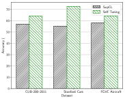
(a) Compare with SupCL

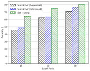
(b) Compare with SimCLRv2

Figure 5: The classification accuracy of various methods when comparing the proposed Self-Tuning with SupCL and SimCLRv2: (a) Compare with SupCL on various datasets provided with a label ratio of $15\%$; (b) Compare with SimCLRv2 on CUB-200-2011 of various label ratios: $15\%$, $30\%$ and $50\%$.

Discussion: Compare with SimCLRv2

In Section 1, we hypothesize that the sequential form between first fine-tuning on $\mathcal{L}$ and then distilling on $\mathcal{U}$ that SimCLRv2 adopts is to blame since the fine-tuned model would easily shift towards the limited labeled data with sampling bias and leaves away from the original smooth model pre-trained on a large-scale dataset. Here, an intuitive idea is to change the sequential form of SimCLRv2 into an intermixed version. As shown in Figure 5(b), we compare Self-Tuning to SimCLRv2 and see an obvious improvement of the intermixed form over the sequential form. However, both forms of SimCLRv2 still much worse than Self-Tuning.

Table 2: Error rates (%) $\downarrow$ on standard SSL benchmark: CIFAR-100 provided with only $400$ labels, $2500$ labels and $10000$ labels.

Method	Network	$2.5$k	$10$k
$\Pi$-Model	WRN-28-8	57.25	37.88
Pseudo-Labeling		57.38	36.21
Mean Teacher	#Para: 11.76M	53.91	35.83
MixMatch		39.94	28.31
UDA		33.13	24.50
ReMixMatch		27.43	23.03
FixMatch		28.64	23.18
FixMatch	EfficientNet-B2	29.99	21.69
Fine-Tuning		31.69	21.74
Co-Tuning	#Para: 9.43M	30.94	22.22
Self-Tuning		24.16	17.57

Table 3: Error rates (%) $\downarrow$ on CIFAR-100 provided with only $400$ labels and a pre-trained EfficientNet-B2 model (CT: Co-Tuning; PL: PseudoLabel; MT: MeanTeacher; FM: FixMatch.)

Fine-Tuning	L2SP	DELTA	BSS	Co-Tuning
60.79	59.21	58.23	58.49	57.58
$\Pi$-model	PseudoLabel	MeanTeacher	FixMatch	UDA
60.50	59.21	60.68	57.87	58.32
SimCLRv2	CT+PL	CT+MT	CT+FM	Self-Tuning
59.45	56.21	56.78	57.94	47.17

5.3 Standard Semi-supervised Learning Benchmarks

We adopt the most difficult CIFAR-100 dataset with $100$ categories among the famous SSL benchmarks including CIFAR-100, CIFAR-10, SVHN, and STL-10, where the last three datasets have only $10$ categories. Since a WRN-28-8 (Zagoruyko & Komodakis, 2016) model pre-trained on ImageNet is not openly available, we adopt an EfficientNet-B2 model with much fewer parameters instead. As shown in Table 2 and Table 3, FixMatch works worse on EfficientNet-B2 than on WRN-28-8, while Self-Tuning outperforms the strongest baselines on WRN-28-8 by large margins. For a fair comparison, we further provided all baselines on EfficientNet-B2 to verify the superiority of Self-Tuning.

Table 4: Classification accuracy (%) $\uparrow$ with a typical unsupervised pre-trained model MoCov2 on CUB-200-2011.

Type	Method	$800$ labels	$5$k labels
TL	Fine-Tuning (baseline)	20.04	71.50
	Co-Tuning	20.99	71.61
SSL	Mean Teacher	28.13	71.26
	FixMatch	21.18	71.28
Combine	Co-Tuning + Mean Teacher	28.43	72.21
	Co-Tuning + FixMatch	21.08	71.40
	Self-Tuning (ours)	36.80	74.56

Table 5: Ablation studies of Self-Tuning on Stanford Cars.

Perspective	Method	15%	30%
Loss Function	w/ CE loss	40.93	67.02
	w/ CL loss	46.29	68.82
	w/ PGC loss	72.50	83.58
Info. Exploration	w/o $\widehat{L}_{\text{PGC}}$	58.82	81.71
	w/o $L_{\text{PGC}}$	58.85	77.52
	separate queue	70.43	80.78
	unified exploration	72.50	83.58

5.4 Unsupervised Pre-trained Models

Besides initializing from supervised pre-trained models, we further explore the performance of Self-Tuning transferring on an unsupervised pre-trained model named MoCov2 (He et al., 2020). As reported in Table 4, Self-Tuning yields consistent gains over SSL and TL methods, revealing that Self-Tuning is not bound to specific pre-trained pretext tasks.

5.5 Named Entity Recognition

We conduct experiments on CoNLL 2003 (Sang & Meulder, 2003), an English named entity recognition (NER) task as a token-level classification problem, to explore the performance of Self-Tuning on NLP tasks. Following the protocol of Co-Tuning, we also adopt BERT (Devlin et al., 2018) as the pre-trained model (masked language modeling one). Measured by the F1-score of named entities, the vanilla fine-tuning baseline achieves an F1-score of $90.81$, BSS, L2-SP and Co-Tuning achieve $90.85$, $91.02$ and $91.27$ respectively, while Self-Tuning achieves a new state-of-the-art of $94.53$.

5.6 Ablation Studies

We conduct ablation studies in Table 5 from two perspectives: (a) Loss Function Type: the assumption in Section 4.1 that PGC loss is much better than CE loss and CL loss for data-efficient deep learning is empirically verified here. (b) Information Exploration Type: by comparing Self-Tuning with models without PGC loss on $\mathcal{L}$ or $\mathcal{U}$, and a model with separate queue lists for $\mathcal{L}$ and $\mathcal{U}$, we demonstrate that the unified exploration is the best choice.

5.7 Sensitivity Analysis

Different from most self-training methods, Self-Tuning is free of confidence-threshold hyper-parameter $t$ and trade-off coefficients between various losses. However, it still has two hyper-parameters: feature size $L$ of the projector head $h$ and queue size $D$ for each category, by introducing a pseudo group contrast mechanism. As shown in Figure 6, Self-Tuning is robust to different values of $L$ and $D$ but tends to prefer larger values of them.

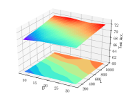
(a) Acc on Car with $15\%$ labels

(b) Acc on Car with $30\%$ labels

Figure 6: Sensitivity analysis for embedded size $L$ of the projector and queue size $D$ of each class on Stanford Cars. (Warmer colors indicate higher values)

(a) Training Process on CUB30

(b) ${\rm Acc}_{\rm test}-{\rm Acc}_{\rm pseudo\_labels}$

Figure 7: Comparisons between Self-Tuning with FixMatch on pseudo label accuracy and test accuracy.

5.8 Why Self-Tuning Works

First, by unifying the exploration of labeled and unlabeled data and the transfer of a pre-trained model, Self-Tuning escapes from the dilemma of just developing TL or SSL methods. Further, Figure 7 reveals that the proposed PGC mechanism successfully boosts the tolerance to false labels, since Self-Tuning has a larger improvement over the accuracy of pseudo-labels than FixMatch, given an identical pre-trained model with approximate pseudo-label accuracy.

6 Conclusion

Mitigating the requirement for labeled data is a vital issue in deep learning community. However, common practices of TL and SSL only focus on either the pre-trained model or unlabeled data. This paper unleashes the power of both of them by proposing a new setup named data-efficient deep learning. To address the challenge of confirmation bias in self-training, a general Pseudo Group Contrast mechanism is devised to mitigate the reliance on pseudo-labels and boost the tolerance to false labels. To tackle the model shift problem, we unify the exploration of labeled and unlabeled data and the transfer of a pre-trained model, with a shared key queue beyond just ‘parallel training’.

References

- Agrawal et al. (2014) Agrawal, P., Girshick, R. B., and Malik, J. Analyzing the performance of multilayer neural networks for object recognition. In ECCV, 2014.
- Arazo et al. (2020) Arazo, E., Ortego, D., Albert, P., O’Connor, N. E., and McGuinness, K. Pseudo-labeling and confirmation bias in deep semi-supervised learning, 2020.
- Brown et al. (2020) Brown, T. B., Mann, B., Ryder, N., Subbiah, M., Kaplan, J., Dhariwal, P., Neelakantan, A., Shyam, P., Sastry, G., Askell, A., Agarwal, S., Herbert-Voss, A., Krueger, G., Henighan, T., Child, R., Ramesh, A., Ziegler, D. M., Wu, J., Winter, C., Hesse, C., Chen, M., Sigler, E., Litwin, M., Gray, S., Chess, B., Clark, J., Berner, C., McCandlish, S., Radford, A., Sutskever, I., and Amodei, D. Language models are few-shot learners. NeurIPS, 2020.
- Chen et al. (2020a) Chen, T., Kornblith, S., Norouzi, M., and Hinton, G. A Simple Framework for Contrastive Learning of Visual Representations. ICML, 2020a.
- Chen et al. (2020b) Chen, T., Kornblith, S., Swersky, K., Norouzi, M., and Hinton, G. Big self-supervised models are strong semi-supervised learners. NeurIPS, 2020b.
- Chen et al. (2019) Chen, X., Wang, S., Fu, B., Long, M., and Wang, J. Catastrophic forgetting meets negative transfer: Batch spectral shrinkage for safe transfer learning. In NeurIPS, 2019.
- Deng et al. (2009) Deng, J., Dong, W., Socher, R., Li, L.-J., Li, K., and Fei-Fei, L. Imagenet: A large-scale hierarchical image database. In CVPR, pp. 248–255, 2009.
- Devlin et al. (2018) Devlin, J., Chang, M.-W., Lee, K., and Toutanova, K. Bert: Pre-training of deep bidirectional transformers for language understanding. arXiv preprint arXiv:1810.04805, 2018.
- Donahue et al. (2014) Donahue, J., Jia, Y., Vinyals, O., Hoffman, J., Zhang, N., Tzeng, E., and Darrell, T. Decaf: A deep convolutional activation feature for generic visual recognition. In ICML, 2014.
- Garg et al. (2020) Garg, S., Sharma, R. K., and Liang, Y. Simpletran: Transferring pre-trained sentence embeddings for low resource text classification. CoRR, abs/2004.05119, 2020.
- Girshick et al. (2014) Girshick, R. B., Donahue, J., Darrell, T., and Malik, J. Rich feature hierarchies for accurate object detection and semantic segmentation. In CVPR, 2014.
- Grandvalet & Bengio (2004) Grandvalet, Y. and Bengio, Y. Semi-supervised learning by entropy minimization. In NeurIPS, 2004.
- He et al. (2016) He, K., Zhang, X., Ren, S., and Sun, J. Deep residual learning for image recognition. In CVPR, pp. 770–778, 2016.
- He et al. (2019) He, K., Girshick, R. B., and Dollár, P. Rethinking imagenet pre-training. In ICCV, 2019.
- He et al. (2020) He, K., Fan, H., Wu, Y., Xie, S., and Girshick, R. Momentum contrast for unsupervised visual representation learning. In CVPR, 2020.
- Houlsby et al. (2019) Houlsby, N., Giurgiu, A., Jastrzebski, S., Morrone, B., de Laroussilhe, Q., Gesmundo, A., Attariyan, M., and Gelly, S. Parameter-efficient transfer learning for NLP. In ICML, 2019.
- Khosla et al. (2020) Khosla, P., Teterwak, P., Wang, C., Sarna, A., Tian, Y., Isola, P., Maschinot, A., Liu, C., and Krishnan, D. Supervised contrastive learning. NeurIPS, 2020.
- Krause et al. (2013) Krause, J., Stark, M., Deng, J., and Fei-Fei, L. 3d object representations for fine-grained categorization. In 4th International IEEE Workshop on 3D Representation and Recognition (3dRR-13), Sydney, Australia, 2013.
- Krizhevsky & Hinton (2009) Krizhevsky, A. and Hinton, G. Learning multiple layers of features from tiny images. Master’s thesis, Department of Computer Science, University of Toronto, 2009.
- Laine & Aila (2017) Laine, S. and Aila, T. Temporal ensembling for semi-supervised learning. In ICLR, 2017.
- Lee (2013) Lee, D. Pseudo-label: The simple and efficient semi-supervised learning method for deep neural networks. In ICML Workshop on Challenges in Representation Learning, 2013.
- Li et al. (2018) Li, X., Grandvalet, Y., and Davoine, F. Explicit inductive bias for transfer learning with convolutional networks. In ICML, 2018.
- Li et al. (2019) Li, X., Xiong, H., Wang, H., Rao, Y., Liu, L., and Huan, J. Delta: Deep learning transfer using feature map with attention for convolutional networks. In ICLR, 2019.
- Maji et al. (2013) Maji, S., Rahtu, E., Kannala, J., Blaschko, M. B., and Vedaldi, A. Fine-grained visual classification of aircraft. Technical report, 2013.
- Oquab et al. (2014) Oquab, M., Bottou, L., Laptev, I., and Sivic, J. Learning and transferring mid-level image representations using convolutional neural networks. In CVPR, 2014.
- Raghu et al. (2019) Raghu, M., Zhang, C., Kleinberg, J. M., and Bengio, S. Transfusion: Understanding transfer learning for medical imaging. In NeurIPS, 2019.
- Sang & Meulder (2003) Sang, E. F. T. K. and Meulder, F. D. Introduction to the conll-2003 shared task: Language-independent named entity recognition. In NAACL, 2003.
- Sohn et al. (2020) Sohn, K., Berthelot, D., Li, C.-L., Zhang, Z., Carlini, N., Cubuk, E. D., Kurakin, A., Zhang, H., and Raffel, C. Fixmatch: Simplifying semi-supervised learning with consistency and confidence. NeurIPS, 2020.
- Sun et al. (2019) Sun, C., Qiu, X., Xu, Y., and Huang, X. How to fine-tune BERT for text classification? In CCL, 2019.
- Tan & Le (2019) Tan, M. and Le, Q. V. Efficientnet: Rethinking model scaling for convolutional neural networks. ICML, 2019.
- Tarvainen & Valpola (2017) Tarvainen, A. and Valpola, H. Mean teachers are better role models: Weight-averaged consistency targets improve semi-supervised deep learning results. In NeurIPS, 2017.
- van den Oord et al. (2018) van den Oord, A., Li, Y., and Vinyals, O. Representation learning with contrastive predictive coding, 2018.
- Wah et al. (2011) Wah, C., Branson, S., Welinder, P., Perona, P., and Belongie, S. The Caltech-UCSD Birds-200-2011 Dataset. Technical Report CNS-TR-2011-001, California Institute of Technology, 2011.
- Wang et al. (2019) Wang, R., Su, H., Wang, C., Ji, K., and Ding, J. To tune or not to tune? how about the best of both worlds? CoRR, 2019.
- Wei et al. (2021) Wei, C., Shen, K., Chen, Y., and Ma, T. Theoretical analysis of self-training with deep networks on unlabeled data. In ICLR, 2021.
- Wu et al. (2018) Wu, Z., Xiong, Y., Yu, S. X., and Lin, D. Unsupervised feature learning via non-parametric instance discrimination. In CVPR, 2018.
- Xie et al. (2020) Xie, Q., Dai, Z., Hovy, E., Luong, M.-T., and Le, Q. V. Unsupervised data augmentation for consistency training. NeurIPS, 2020.
- Yarowsky (1995) Yarowsky, D. Unsupervised word sense disambiguation rivaling supervised methods. In ACL, 1995.
- Yosinski et al. (2014) Yosinski, J., Clune, J., Bengio, Y., and Lipson, H. How transferable are features in deep neural networks? In NeurIPS, 2014.
- You et al. (2020) You, K., Kou, Z., Long, M., and Wang, J. Co-tuning for transfer learning. Advances in Neural Information Processing Systems, 33, 2020.
- Zagoruyko & Komodakis (2016) Zagoruyko, S. and Komodakis, N. Wide residual networks. CoRR, abs/1605.07146, 2016.