Hyperbolic relaxation technique for solving the dispersive Serre–Green–Naghdi equations with topography

Abstract

The objective of this paper is to propose a hyperbolic relaxation technique for the dispersive Serre–Green–Naghdi equations (also known as the fully non-linear Boussinesq equations) with full topography effects introduced in Green and Naghdi [14] and Seabra-Santos et al. [24]. This is done by revisiting a similar relaxation technique introduced in Guermond et al. [17] with partial topography effects. We also derive a family of analytical solutions for the one-dimensional dispersive Serre–Green–Naghdi equations that are used to verify the correctness the proposed relaxed model. The method is then numerically illustrated and validated by comparison with experimental results.

65M60, 65M12, 35L50, 35L65, 76M10

1 Introduction

The Saint -Venant shallow water equations model the free surface of a body of water evolving under the action of gravity under the assumptions that the deformation of the free surface is small compared to the water elevation and the bottom topography $z$ varies slowly. Letting $\mu=\frac{\mathsf{h}_{0}^{2}}{L^{2}}$ be the shallowness parameter, where $\mathsf{h}_{0}$ is the typical water height and $L$ is the typical horizontal lengthscale, Saint-Venant’s shallow water model is the ${\mathcal{O}}(\mu)$ approximation of the free surface Euler equations. This is a hyperbolic system that has many practical applications, but one of its main deficiencies is that it does not have dispersive properties. In particular, it does not support smooth solitary waves. A model that includes all the first-order correction in terms of the shallowness parameter (i.e., it is a ${\mathcal{O}}(\mu^{2})$ approximation of the free surface incompressible Euler equations) has been introduced by Serre [25, Eq. (22), p. 860] with a flat topography. This model has been rediscovered verbatim in Su and Gardner [26], and rediscovered again in Green et al. [15] also with flat topography. The key property of this model (as unequivocally recognized and illustrated in [25, §2]) is that it supports smooth solitary waves. The model has been further improved in Seabra-Santos et al. [24, Eq. (13)] and Green and Naghdi [14, Eq. (4.27)–(4.31)] to include the effects of topography up to the order ${\mathcal{O}}(\mu^{2})$. We refer the reader to Barthélemy [2] and Lannes [21] for comprehensive reviews of the properties of the model. All these works based on informal asymptotic expansions have been rigorously formalised in Alvarez-Samaniego and Lannes [1, Thm 6.2]. For brevity, we refer to the Serre–Green–Nagdhi equations as just the Serre model.

One major drawback of the dispersive Serre model from a numerical perspective is that it involves third-order derivatives in space. The presence of the third-order derivatives rules out any approximation technique that is explicit in time, since this would require the time step ${\tau}$ to behave like ${\mathcal{O}}(h^{3})V^{-1}L^{-2}$, where $h$ is the mesh-size, $V$ is a characteristic wave speed scale, and $L$ is a characteristic length scale. There are currently two popular classes of techniques for addressing this difficulty. The first one is based on Stang’s operator splitting and combines explicit and implicit time stepping, see for instance Bonneton et al. [5], Samii and Dawson [23], Duran and Marche [9]. Another approach consists of reinterpreting the dispersive system as a constrained first-order system and then relaxing the constraint, see for instance Favrie and Gavrilyuk [11], Tkachenko [27], Guermond et al. [17], and Escalante et al. [10]. Note that the technique in Escalante et al. [10] is based on a dispersive model introduced in Bristeau et al. [7] which differs from the Serre model up to a multiplicative constant when the topography is flat (their pressure constant is $\tfrac{1}{4}$ as opposed to the Serre constant $\tfrac{1}{3}$). All the above relaxation techniques are, however, incomplete since they ignore the topography corrections introduced in [14, 24]. These terms play an important role in modeling the effects of vertical acceleration due to the topography and are necessary for correctly reproducing laboratory experiments. A recent hyperbolic reformulation with topography effects was introduced in Bassi et al. [3] which was based on the work of  Fernandez-Nieto et al. [12] (where the reformulation uses a constraint on the divergence of the velocity).

In the present paper we exclusively focus on the topography corrections. By revisiting the experiments reported in Seabra-Santos et al. [24], we unambiguously demonstrate that the topography corrections are indeed important to reproduce experiment involving reflected waves (see Table 3). We also show that the Serre model with topography effects can be reformulated as a constrained first-order system. We propose a relaxation technique that makes the system hyperbolic and, thereby, allows for explicit time stepping under reasonable time step restrictions. The key difference with our previous work in [17] is now the presence of the topography effects in the pressure and extra topography source terms which make the analysis more involved: there is one more conservation equation and one more relaxation term has to be added; the source terms in the additional conservation equations have to be modified appropriately to be compatible with the global energy conservation equation.

The paper is organized as follows. In Section 2, we recall the dispersive Serre model with topography and state the corresponding energy conservation equation. We also derive a family of analytical solutions to the one-dimensional system. To the best of our knowledge, it is the first time that an exact solution to this nonlinear system of equations is proposed when the topography is nontrivial. This solution is not a manufactured solution since it does not involve any ad hoc source terms. The main interest of this exact solution is to help verify numerical codes for the approximation of the dispersive Serre model with topography (which, to the best of our knowledge, was done in the literature only with manufactured solutions involving ad hoc source terms). In Section 3, we reformulate the dispersive Serre model as a first-order system of nonlinear conservation equations with two algebraic constraints. We then relax these constraints and propose a hyperbolic system of equations that allows for explicit time stepping and is compatible with dry states. This system is shown to admit an energy equation. Finally, in Section 4, we illustrate the proposed model. Using a continuous finite element technique, we compare the new method with that described in [17] (where the model is incomplete because the topography correction terms from [14, 24] are not accounted for). We also compare the new method with several laboratory experiments in one and two spatial dimensions and unequivocally conclude that the topography effects are important to reproduce the experiments.

2 Dispersive Serre model with topography

In this section we recall the dispersive Serre model with topography and derive an exact solution to the one-dimensional steady state problem.

2.1 The dispersive model

Let ${\bm{u}}=(\mathsf{h},{\bm{q}})^{\mathsf{T}}$ be the dependent variable, where $\mathsf{h}$ is the water height and ${\bm{q}}$ is the flow rate, or discharge. The dispersive Serre model with topography effects is written as follows:

(2.1) $$\partial_{t}{\bm{u}}+\nabla{\cdot}{\mathbbm{f}}({\bm{u}})+{\bm{b}}({\bm{u}},\nabla z)=\bm{0},\quad\text{a.e.\@\ }{\bm{x}}\in D,\ t\in{\mathbb{R}}_{+}.$$

The flux ${\mathbbm{f}}({\bm{u}})$ and the bathymetry source ${\bm{b}}({\bm{u}},\nabla z)$ are given by

(2.2) $$\quad{\mathbbm{f}}({\bm{u}}):=\left(\begin{matrix}{\bm{q}}^{\mathsf{T}}\\ \frac{1}{\mathsf{h}}{\bm{q}}{\otimes}{\bm{q}}+p({\bm{u}}){\mathbb{I}}_{d}\end{matrix}\right)\in{\mathbb{R}}^{(1+d)\times d},\quad{\bm{b}}({\bm{u}},\nabla z):=\left(\begin{matrix}0\\ r({\bm{u}})\nabla z\end{matrix}\right),$$

with the pressure $p({\bm{u}})$ and the source $r({\bm{u}})$ defined by

(2.3a) $$p({\bm{u}}):=\tfrac{1}{2}g\mathsf{h}^{2}+\mathsf{h}^{2}\Big{(}\tfrac{1}{3}\ddot{\mathsf{h}}+\tfrac{1}{2}\dot{\mathsf{k}}\Big{)}, \dot{\mathsf{h}}:=\partial_{t}\mathsf{h}+{\bm{v}}{\cdot}\nabla\mathsf{h},\qquad\ddot{\mathsf{h}}:=\partial_{t}\dot{\mathsf{h}}+{\bm{v}}{\cdot}\nabla\dot{\mathsf{h}},$$

(2.3b) $$r({\bm{u}})=g\mathsf{h}+\mathsf{h}\Big{(}\tfrac{1}{2}\ddot{\mathsf{h}}+\dot{\mathsf{k}}\Big{)}, \dot{\mathsf{k}}:=\partial_{t}({\bm{v}}{\cdot}\nabla z)+{\bm{v}}{\cdot}\nabla({\bm{v}}{\cdot}\nabla z).$$

Here the vector field ${\bm{v}}$ is the velocity and is defined by ${\bm{v}}:=\frac{1}{\mathsf{h}}{\bm{q}}$. Due to the presence of the term $\tfrac{1}{2}\ddot{\mathsf{h}}+\dot{\mathsf{k}}$, the pressure mapping ${\bm{u}}\mapsto p({\bm{u}})$ is not a function but a second-order differential operator in space and time. This implies that (2.1)–(2.3) is not a quasilinear first-order system. In this paper we exclusively focus our attention on the terms $\tfrac{1}{2}\mathsf{h}^{2}\dot{\mathsf{k}}$ in $p({\bm{u}})$ and $\dot{\mathsf{k}}$ in ${\bm{r}}({\bm{u}})$, which are the ${\mathcal{O}}(\mu^{2})$ contributions induced by the topography identified in Green and Naghdi [14] and Seabra-Santos et al. [24].

Notice that the mass conservation equation implies $\dot{\mathsf{h}}=-\mathsf{h}\nabla{\cdot}{\bm{v}}$, which in turn implies that $\ddot{\mathsf{h}}=-\partial_{t}(\mathsf{h}\nabla{\cdot}{\bm{v}})-{\bm{v}}{\cdot}\nabla(\mathsf{h}\nabla{\cdot}{\bm{v}})$. This means that the term $\mathsf{h}^{2}\ddot{\mathsf{h}}$ in the pressure equation (2.3a) can also be rewritten as $-\mathsf{h}^{3}(\partial_{t}\nabla{\cdot}{\bm{v}}+{\bm{v}}{\cdot}\nabla(\nabla{\cdot}{\bm{v}})-(\nabla{\cdot}{\bm{v}})^{2})$, which is exactly the expression given in Serre [25, Eq. (22), p. 860] and Su and Gardner [26, A14] twenty-one and five years earlier, respectively, than Green et al. [15, Eq. (4.16)–(4.19)].

One important result we are going to use is that the system (2.1)–(2.3) admits an energy equation if the solution is smooth.

Lemma 2.1.

Let ${\bm{u}}$ be a smooth solution to (2.1)–(2.3), then the following holds true: $\partial_{t}{\mathcal{E}}({\bm{u}})+\nabla{\cdot}(\bm{{\mathcal{F}}}({\bm{u}}))=0$, with

(2.4a) $${\mathcal{E}}({\bm{u}}) :=\tfrac{1}{2}g{\color[rgb]{0,0,1}(\mathsf{h}+z)^{2}}+\tfrac{1}{2}\mathsf{h}{\bm{v}}^{2}+\tfrac{1}{6}\mathsf{h}\Big{(}\big{(}\dot{\mathsf{h}}+\tfrac{3}{2}({\bm{v}}{\cdot}\nabla z)\big{)}^{2}+\tfrac{3}{4}({\bm{v}}{\cdot}\nabla z)^{2}\Big{)},$$

(2.4b) $$\bm{{\mathcal{F}}}({\bm{u}}) :={\bm{v}}({\mathcal{E}}({\bm{u}}){\color[rgb]{0,0,1}-\tfrac{1}{2}gz^{2}}+p({\bm{u}})).$$

$\square$

Proof 2.2.

We direct the reader to the proof of Lemma 3.9 for a detailed process on the derivation of the energy equation. Note that the energy (2.4a) is the same as the one reported in Castro and Lannes [8, Eq. (1.19)–(1.22)]. $\square$

2.2 One-dimensional steady-state solution

We now propose a steady-state solution to (2.1)–(2.3) with non-trivial topography. We restrict ourselves to one space dimension and assume that the solution to (2.1)–(2.3) is time-independent and smooth. The following assertion is the main result from this section.

Lemma 2.3.

Let $q\in{\mathbb{R}}$, $a,r\in{\mathbb{R}}_{+}$ and let the bathymetry profile be defined by $z(x):=-\tfrac{1}{2}\frac{a}{(\cosh(rx))^{2}}$. Then $\mathsf{h}(x)=\mathsf{h}_{0}(1+\frac{a}{(\cosh(rx))^{2}})$ with the constant discharge $q$ is a steady state solution to (2.1)–(2.3) if

(2.5) $$q:=\pm\sqrt{\frac{(1+a)g\mathsf{h}_{0}^{3}}{2}},\qquad r:=\frac{1}{\mathsf{h}_{0}}\sqrt{\frac{3a}{(1+a)}}.$$

$\square$

Proof 2.4.

Notice that the discharge $q$ is constant since the solution does not depend on time. A steady-state solution can be found by solving the steady-state problem of the energy equation in Lemma 2.1; this yields a Bernoulli-like relation for the dispersive Serre model (2.1)–(2.3). More precisely, from Lemma 2.1, we infer that $\partial_{x}({\mathcal{F}}({\bm{u}}))=0$, which implies ${\mathcal{F}}({\bm{u}}(x))=C_{\text{Ber}}gq$ where $C_{\text{Ber}}$ is the Bernoulli constant. We look for a stationary wave with the following structure $\mathsf{h}(x)=\mathsf{h}_{0}(1+\frac{a}{(\cosh(rx))^{2}})$ and posit that the topography is of the form $z(x)=\lambda(\mathsf{h}(x)-\mathsf{h}_{0})$. The problem now consists of finding relations between the parameters $a$, $r$, $\mathsf{h}_{0}$, $g$, and $\lambda$ so that the condition $g^{-1}q^{-1}{\mathcal{F}}({\bm{u}}(x))=C_{\text{Ber}}$ is satisfied, i.e.,

$$\mathsf{h}(1+\lambda)+\frac{q^{2}}{2g\mathsf{h}^{2}}-\frac{q^{2}}{6g\mathsf{h}^{2}}(1-3\lambda^{2})(\partial_{x}\mathsf{h})^{2}+\frac{q^{2}}{3g\mathsf{h}}(1+\tfrac{3}{2}\lambda)\partial_{xx}\mathsf{h}=C_{\text{Ber}}+\lambda\mathsf{h}_{0},$$

where we used $v=\frac{q}{\mathsf{h}}$. By taking the limit of this identity for $|x|\to\infty$, we find that $C_{\text{Ber}}=\mathsf{h}_{0}+\frac{q^{2}}{2g\mathsf{h}_{0}^{2}}.$ After inserting the ansatz $\mathsf{h}(x)=\mathsf{h}_{0}(1+\frac{a}{(\cosh(rx))^{2}})$ into the above identity, we find that the following must hold true for all $x\in{\mathbb{R}}$:

$$\big{(}(1+\lambda)g\mathsf{h}_{0}^{3}+(\lambda+\tfrac{2}{3})2r^{2}q^{2}\mathsf{h}_{0}^{2}-q^{2}\big{)}\cosh(rx)^{4}\\ +\big{(}(1+\lambda)2ag\mathsf{h}_{0}^{3}+((\lambda^{2}+\lambda+\tfrac{1}{3})a-\tfrac{3}{2}\lambda-1)2r^{2}q^{2}\mathsf{h}_{0}^{2}-\tfrac{1}{2}aq^{2}\big{)}\cosh(rx)^{2}\\ +\big{(}(1+\lambda)ag\mathsf{h}_{0}-2(\lambda^{2}+\tfrac{3}{2}\lambda+\tfrac{2}{3})r^{2}q^{2}\big{)}a\mathsf{h}_{0}^{2}=0.$$

This is equivalent to asserting that following nonlinear system of equations has a solution:

$$(1+\lambda)ag\mathsf{h}_{0}-2(\lambda^{2}+\tfrac{3}{2}\lambda+\tfrac{2}{3})r^{2}q^{2} =0,$$

$$(1+\lambda)2ag\mathsf{h}_{0}^{3}+((\lambda^{2}+\lambda+\tfrac{1}{3})a-\tfrac{3}{2}\lambda-1)2r^{2}q^{2}\mathsf{h}_{0}^{2}-\tfrac{1}{2}aq^{2} =0,$$

$$(1+\lambda)g\mathsf{h}_{0}^{3}+(\lambda+\tfrac{2}{3})2r^{2}q^{2}\mathsf{h}_{0}^{2}-q^{2} =0.$$

The only nontrivial solution we have found is $\lambda=-\tfrac{1}{2}$ with $q$ and $r$ satisfying (2.5). $\square$

It seems that the solution formulated in Lemma 2.3 is the first exact solution to the nonlinear system (2.1)–(2.3) proposed in the literature when the topography is nontrivial. Our motivation to construct this solution was mainly to verify convergence of numerical codes solving (2.1)–(2.3).

3 Reformulation of the dispersive Serre model

In this section, we reformulate the dispersive Serre model as a first-order system under two algebraic constraints. Our goal is to introduce a relaxation technique in the spirit of Guermond et al. [17].

3.1 Reformulation

The analysis done in [17] is incomplete since it does not account for the dispersion terms induced by the topography. We now revisit [17] to fill in the gap and account for the missing terms. The main result of this section is the following.

Lemma 3.1.

Let ${\bm{u}}:D{\times}(0,T)\to{\mathbb{R}}_{+}{\times}{\mathbb{R}}^{d}$ be a smooth function. Then ${\bm{u}}$ solves the dispersive Serre model (2.1)–(2.3) iff $({\bm{u}},q_{1},q_{2},q_{3})$ solves

(3.1a) $$\partial_{t}\mathsf{h}+\nabla{\cdot}{\bm{q}}=0,$$

(3.1b) $$\partial_{t}{\bm{q}}+\nabla{\cdot}({\bm{v}}\otimes{\bm{q}})+\nabla(\tfrac{1}{2}g\mathsf{h}^{2}-\tfrac{1}{3}\mathsf{h}s)=-(g\mathsf{h}-\tfrac{1}{2}s+\tfrac{1}{4}{\widetilde{s}})\nabla z,$$

(3.1c) $$\partial_{t}q_{1}+\nabla{\cdot}({\bm{v}}q_{1})=q_{2}-\tfrac{3}{2}q_{3},$$

(3.1d) $$\partial_{t}q_{2}+\nabla{\cdot}({\bm{v}}q_{2})=-s,$$

(3.1e) $$\partial_{t}q_{3}+\nabla{\cdot}({\bm{v}}q_{3})={\widetilde{s}},$$

(3.1f) $$q_{1}=\mathsf{h}^{2},\quad q_{3}={\bm{q}}{\cdot}\nabla z.$$

$\square$

Proof 3.2.

Assume that ${\bm{u}}$ solves (2.1)–(2.3). We are going to show that ${\bm{u}}:=(\mathsf{h},{\bm{q}})$ solves (3.1a)-(3.1f).
(i) Let $q_{1}:=\mathsf{h}^{2}$ and $q_{3}:={\bm{q}}{\cdot}\nabla z$ be defined as in (3.1f). In addition, let us set $q_{2}:=-\mathsf{h}^{2}\nabla{\cdot}{\bm{v}}+\tfrac{3}{2}q_{3}$. Using the mass conservation equation, these definitions imply that

$$\partial_{t}q_{1}+\nabla{\cdot}({\bm{v}}q_{1}) =\partial_{t}\mathsf{h}^{2}+\nabla{\cdot}({\bm{v}}\mathsf{h}^{2})=\mathsf{h}\partial_{t}\mathsf{h}+\mathsf{h}{\bm{v}}{\cdot}\nabla\mathsf{h}=-\mathsf{h}^{2}\nabla{\cdot}{\bm{v}}=q_{2}-\tfrac{3}{2}q_{3}.$$

Hence (3.1c) holds true.
(ii) Let us define ${\widetilde{s}}:=\partial_{t}q_{3}+\nabla{\cdot}({\bm{v}}q_{3})$ and $s:=-\mathsf{h}\ddot{\mathsf{h}}-\tfrac{3}{2}{\widetilde{s}}$. Using again mass conservation and the identity $q_{2}=\mathsf{h}\dot{\mathsf{h}}+\tfrac{3}{2}q_{3}$ (recall that $\dot{\mathsf{h}}=-\mathsf{h}\nabla{\cdot}{\bm{v}}$), we infer that

$$\partial_{t}q_{2}+\nabla{\cdot}({\bm{v}}q_{2}) =\mathsf{h}(\partial_{t}\dot{\mathsf{h}}+{\bm{v}}{\cdot}\nabla\dot{\mathsf{h}})+\tfrac{3}{2}(\partial_{t}q_{3}+\nabla{\cdot}({\bm{v}}q_{3}))=\mathsf{h}\ddot{\mathsf{h}}+\tfrac{3}{2}{\widetilde{s}}=-s.$$

This shows that (3.1d) holds true. Notice also that (3.1e) holds true as well since this is the definition of ${\widetilde{s}}$.
(iii) Recalling that we have defined $q_{3}:=\mathsf{h}{\bm{v}}{\cdot}\nabla z$, the definition of $\dot{{\mathsf{k}}}$ in (2.3b) gives $\mathsf{h}\dot{{\mathsf{k}}}=\partial_{t}q_{3}+\nabla{\cdot}({\bm{v}}q_{3})={\widetilde{s}}$. Then, using that $s:=-\mathsf{h}\ddot{\mathsf{h}}-\tfrac{3}{2}{\widetilde{s}}$, the pressure defined in (2.3a) is rewritten as follows:

$$p({\bm{u}}) =\tfrac{1}{2}g\mathsf{h}^{2}+\mathsf{h}(\tfrac{1}{3}\mathsf{h}\ddot{\mathsf{h}}+\tfrac{1}{2}\mathsf{h}\dot{\mathsf{k}})=\tfrac{1}{2}g\mathsf{h}^{2}+\mathsf{h}(\tfrac{1}{3}\mathsf{h}\ddot{\mathsf{h}}+\tfrac{1}{2}{\widetilde{s}})$$

$$=\tfrac{1}{2}g\mathsf{h}^{2}+\tfrac{1}{3}\mathsf{h}(\mathsf{h}\ddot{\mathsf{h}}+\tfrac{3}{2}{\widetilde{s}})=\tfrac{1}{2}g\mathsf{h}^{2}-\tfrac{1}{3}\mathsf{h}s.$$

This is exactly the form of the pressure term in (3.1b). Moreover, using that $\mathsf{h}\dot{{\mathsf{k}}}={\widetilde{s}}$ and $\mathsf{h}\ddot{\mathsf{h}}=-s-\tfrac{3}{2}{\widetilde{s}}$, the source term induced by the topography in (2.3b), $r({\bm{u}})$, becomes

$$r({\bm{u}})=g\mathsf{h}+\mathsf{h}(\tfrac{1}{2}\ddot{\mathsf{h}}+\dot{{\mathsf{k}}})=g\mathsf{h}-\tfrac{1}{2}s-\tfrac{3}{4}{\widetilde{s}}+{\widetilde{s}}=g\mathsf{h}-\tfrac{1}{2}s+\tfrac{1}{4}{\widetilde{s}}.$$

i.e., we obtain $r({\bm{u}})\nabla z=(g\mathsf{h}-\tfrac{1}{2}s+\tfrac{1}{4}{\widetilde{s}})\nabla z$, which is exactly the form of the source term in (3.1b). In conclusion, we have established that (3.1a) to (3.1f) hold true if ${\bm{u}}$ solves (2.1)–(2.3).

We now prove the converse. Let us assume that $({\bm{u}},q_{1},q_{2},q_{3})$ solves (3.1a)–(3.1f).
(iv) Again we set ${\bm{u}}:=(\mathsf{h},{\bm{q}})$ and ${\bm{v}}:=\mathsf{h}^{-1}{\bm{q}}$. Let us set $\dot{\mathsf{k}}:=\partial_{t}({\bm{v}}{\cdot}\nabla z)+{\bm{v}}{\cdot}\nabla({\bm{v}}{\cdot}\nabla z)$. Then using (3.1e) and (3.1f) we obtain $\mathsf{h}\dot{\mathsf{k}}={\widetilde{s}}$. Similarly, mass conservation implies that $\mathsf{h}\dot{\mathsf{h}}=\partial_{t}(\mathsf{h}^{2})+\nabla{\cdot}({\bm{v}}\mathsf{h}^{2})$. This identity, together with $q_{1}:=\mathsf{h}^{2}$ and (3.1c), gives $\mathsf{h}\dot{\mathsf{h}}=q_{2}-\tfrac{3}{2}q_{3}$. Then

$$\mathsf{h}\ddot{\mathsf{h}}=\partial_{t}(\mathsf{h}\dot{\mathsf{h}})+\nabla{\cdot}({\bm{v}}\mathsf{h}\dot{\mathsf{h}})=\partial_{t}(q_{2}-\tfrac{3}{2}q_{3})+\nabla{\cdot}({\bm{v}}(q_{2}-\tfrac{3}{2}q_{3}))=-s-\tfrac{3}{2}{\widetilde{s}}.$$

This implies that $s=-\mathsf{h}(\ddot{\mathsf{h}}+\tfrac{3}{2}\dot{\mathsf{k}})$. Let us set $p:=\tfrac{1}{2}g\mathsf{h}^{2}-\tfrac{1}{3}\mathsf{h}s$. Then $p=\tfrac{1}{2}g\mathsf{h}^{2}+\mathsf{h}^{2}(\tfrac{1}{3}\ddot{\mathsf{h}}+\tfrac{1}{2}\dot{\mathsf{k}})$. This is the expression of the pressure in (2.3a).
(v) Finally let us set $r:=g\mathsf{h}-\tfrac{1}{2}s+\tfrac{1}{4}{\widetilde{s}}$. Then the above computations imply that $r=g\mathsf{h}+\tfrac{1}{2}\mathsf{h}(\ddot{\mathsf{h}}+\tfrac{3}{2}\dot{\mathsf{k}})+\tfrac{1}{4}\mathsf{h}\dot{\mathsf{k}}$, i.e., $r=g\mathsf{h}+\tfrac{1}{2}\mathsf{h}\ddot{\mathsf{h}}+\dot{\mathsf{k}}$. This is the expression of the source term $r$ in (2.3b). Hence we have established that ${\bm{u}}$ solves (2.1)–(2.3). This completes the proof. $\square$

The following is another way to reformulate Lemma 3.1, which we exploit in the next section:

Proposition 3.3 (Co-dimension 2).

Let ${\bm{u}}:D{\times}(0,T)\to{\mathbb{R}}_{+}{\times}{\mathbb{R}}^{d}$ be a smooth function. Then ${\bm{u}}$ solves the dispersive Serre model (2.1)–(2.3) if and only if $({\bm{u}},q_{1},q_{2},q_{3})$ solves the quasilinear first-order system (3.1a)–(3.1e) on the co-dimension 2 manifold $\{(\mathsf{h},{\bm{q}},q_{1},q_{2},q_{3})\in{\mathbb{R}}_{+}{\times}{\mathbb{R}}^{d}{\times}{\mathbb{R}}_{+}{\times}{\mathbb{R}}^{2}{\;|\;}q_{1}=\mathsf{h}^{2},\ q_{3}={\bm{q}}{\cdot}\nabla z\}$. $\square$

Remark 3.4 (Initial conditions).

Let $(\mathsf{h}_{0},{\bm{q}}_{0})$ be the initial state for (2.1)–(2.3). Then the corresponding initial state for (3.1a)–(3.1f) is

$$\mathsf{h}({\bm{x}},0)=\mathsf{h}_{0}({\bm{x}}),\qquad\quad{\bm{q}}({\bm{x}},0)={\bm{q}}_{0}({\bm{x}}),\qquad\quad q_{1}({\bm{x}},0)=\mathsf{h}_{0}({\bm{x}})^{2},$$

$$q_{3}({\bm{x}},0)={\bm{q}}_{0}({\bm{x}}){\cdot}\nabla z,\quad q_{2}({\bm{x}},0)=-\mathsf{h}_{0}({\bm{x}})\nabla{\cdot}{\bm{v}}_{0}({\bm{x}})+\tfrac{3}{2}q_{3}({\bm{x}},0).$$

$\square$

3.2 The relaxation

In this section we propose a technique to relax the constraints $\{q_{1}=\mathsf{h}^{2};\ q_{3}={\bm{q}}{\cdot}\nabla z\}$ in (3.1a)–(3.1e) so that the relaxed system becomes hyperbolic and remains compatible with dry states. This is done by adapting arguments introduced in [17] and initially based on ideas from [11].

We use the same notation as in [11] and [17]. The state variable is denoted ${\bm{u}}:=(\mathsf{h},{\bm{q}},q_{1},q_{2},q_{3})$. We set $\eta:=\frac{q_{1}}{\mathsf{h}}$, $\omega:=\frac{q_{2}}{\mathsf{h}}$, and we introduce the new variable $\beta:=\frac{q_{3}}{\mathsf{h}}$. Let $\epsilon$ be a small length scale which we will later think of as being some mesh-size when the model is approximated in space. Let $\overline{\lambda}$ be a non-dimensional number of order unit (say for instance $\overline{\lambda}=1$).

Let $\Gamma\in C^{2}({\mathbb{R}};[0,\infty))$ be a smooth non-negative function such that $\Gamma(1)=0$ and $\Gamma^{\prime}(1)=0$. As in [17] we replace $s$ in (3.1d) by $\overline{\lambda}g\frac{\mathsf{h}^{2}}{\epsilon}\Gamma^{\prime}(\frac{\eta}{\mathsf{h}})$. Notice that $g\frac{\mathsf{h}^{2}}{\epsilon}$ scales like the square of a velocity, which is what one should expect since $-\overline{\lambda}g\frac{\mathsf{h}^{2}}{\epsilon}\Gamma^{\prime}(\frac{\eta}{\mathsf{h}})$ should be an ansatz for $-\mathsf{h}(\ddot{\mathsf{h}}+\tfrac{3}{2}\dot{{\mathsf{k}}})$. The purpose of this term is to enforce the ratio $\frac{\eta}{\mathsf{h}}$ to be close to $1$ (i.e., $q_{1}\rightarrow\mathsf{h}^{2}$ as $\epsilon\to 0$).

Let $\Phi\in C^{0}({\mathbb{R}};{\mathbb{R}})$ be a function such that $\xi\Phi(\xi)\geq 0$ for all $\xi\in{\mathbb{R}}$. Let $\mathsf{h}_{0}$ be a reference water height. We are going to replace ${\widetilde{s}}$ in (3.1e) by $\overline{\lambda}g\mathsf{h}_{0}\frac{\mathsf{h}}{\epsilon}\Phi(({\bm{v}}\cdot\nabla z-\beta)/\sqrt{g\mathsf{h}_{0}})$. The purpose of this term is to enforce $({\bm{v}}{\cdot}\nabla z-\beta)/\sqrt{g\mathsf{h}_{0}}$ to be close to $0$ (i.e., $q_{3}\rightarrow{\bm{q}}\cdot\nabla z$ as $\epsilon\to 0$).

Recalling that ${\bm{v}}:=\mathsf{h}^{-1}{\bm{q}}$, $q_{1}:=\mathsf{h}\eta$, $q_{2}:=\mathsf{h}\omega$ and $q_{3}:=\mathsf{h}\beta$, the relaxed system we consider in the rest of the paper is formulated as follows:

(3.2a) $$\partial_{t}\mathsf{h}+\nabla{\cdot}{\bm{q}}=0,$$

(3.2b) $$\partial_{t}{\bm{q}}+\nabla{\cdot}({\bm{v}}\otimes{\bm{q}})+\nabla p_{\epsilon}({\bm{u}})=-r_{\epsilon}({\bm{u}})\nabla z,$$

(3.2c) $$\partial_{t}q_{1}+\nabla{\cdot}({\bm{v}}q_{1})=q_{2}-\tfrac{3}{2}{\bm{q}}{\cdot}\nabla z,$$

(3.2d) $$\partial_{t}q_{2}+\nabla{\cdot}({\bm{v}}q_{2})=-s_{\epsilon}({\bm{u}}),$$

(3.2e) $$\partial_{t}q_{3}+\nabla{\cdot}({\bm{v}}q_{3})={\widetilde{s}}_{\epsilon}({\bm{u}}),$$

(3.2f) $$p_{\epsilon}({\bm{u}}):=\tfrac{1}{2}g\mathsf{h}^{2}+\widetilde{p}_{\epsilon}({\bm{u}}),\qquad\widetilde{p}_{\epsilon}({\bm{u}}):=-\tfrac{1}{3}\tfrac{\overline{\lambda}g}{\epsilon}\mathsf{h}^{2}\big{(}\eta\Gamma^{\prime}(\tfrac{\eta}{\mathsf{h}})-2\mathsf{h}\Gamma(\tfrac{\eta}{\mathsf{h}})\big{)},$$

(3.2g) $$r_{\epsilon}({\bm{u}}):=g\mathsf{h}-\tfrac{1}{2}s_{\epsilon}({\bm{u}})+\tfrac{1}{4}{\widetilde{s}}_{\epsilon}({\bm{u}}),$$

(3.2h) $$s_{\epsilon}({\bm{u}}):=\overline{\lambda}g\tfrac{\mathsf{h}^{2}}{\epsilon}\Gamma^{\prime}(\tfrac{\eta}{\mathsf{h}}),\qquad\qquad{\widetilde{s}}_{\epsilon}({\bm{u}}):=\overline{\lambda}g\mathsf{h}_{0}\tfrac{\mathsf{h}}{\epsilon}\Phi(\tfrac{{\bm{v}}\nabla z-\beta}{\sqrt{g\mathsf{h}_{0}}}).$$

Remark 3.5 ($q_{3}$).

Notice that we have replaced $-\frac{3}{2}q_{3}$ on the right-hand side of (3.2c) by $-\tfrac{3}{2}{\bm{q}}{\cdot}\nabla z$. This is consistent since $q_{3}$ should be equal to ${\bm{q}}{\cdot}\nabla z$. This change is justified by the energy argument in Lemma 3.9. $\square$

Remark 3.6 (Definition of $\Phi$).

In the applications reported at the end of the paper we take $\Phi(\xi)=\xi$, but we prefer to present the method with a generic function $\Phi$ to emphasize the generality of the relaxation procedure. $\square$

Remark 3.7 (Pressure).

The expression for the pressure $\widetilde{p}_{\epsilon}({\bm{u}})$ in (3.2f) is fully justified by the energy argument in Lemma 3.9. After replacing $s$ by $\overline{\lambda}g\frac{\mathsf{h}^{2}}{\epsilon}\Gamma^{\prime}(\frac{\eta}{\mathsf{h}})$ in (3.1b), we observe that the definition of $\widetilde{p}_{\epsilon}({\bm{u}})$ is compatible with the definition $\widetilde{p}({\bm{u}})=-\frac{1}{3}\mathsf{h}s$ up to the remainder $\frac{1}{3}\frac{\overline{\lambda}g}{\epsilon}2\mathsf{h}^{3}\Gamma(\tfrac{\eta}{\mathsf{h}})$, which indicates that (3.2) may not be consistent with (3.1). This is not the case since this remainder is small when the ratio $\frac{\eta}{\mathsf{h}}$ is close to $1$. More precisely, using Taylor expansions at $1$, we have

$$\Gamma(1)=0=\Gamma(\frac{\eta}{\mathsf{h}})+\mathsf{h}^{-1}(\mathsf{h}-\eta)\Gamma^{\prime}(\frac{\eta}{\mathsf{h}})+\mathsf{h}^{-2}{\mathcal{O}}(\mathsf{h}-\eta)^{2},$$

which shows that $2\mathsf{h}\Gamma(\tfrac{\eta}{\mathsf{h}})/\eta|\Gamma^{\prime}(\frac{\eta}{\mathsf{h}})|={\mathcal{O}}(\tfrac{|\eta-\mathsf{h}|}{\eta})$. Hence the ratio $2\mathsf{h}\Gamma(\tfrac{\eta}{\mathsf{h}})/\eta|\Gamma^{\prime}(\frac{\eta}{\mathsf{h}})|$ is small as $\eta\to\mathsf{h}$, which proves that $\widetilde{p}_{\epsilon}({\bm{u}})$ is indeed a consistent approximation of $\widetilde{p}({\bm{u}})=-\frac{1}{3}\mathsf{h}s$ as $\eta\to\mathsf{h}$. $\square$

Remark 3.8 (Comparisons with [17]).

The incomplete system considered in [17] consists of solving for $(\mathsf{h},{\bm{q}},q_{1},q_{2})^{\mathsf{T}}$ so that

(3.3a) $$\partial_{t}\mathsf{h}+\nabla{\cdot}{\bm{q}}=0,$$

(3.3b) $$\partial_{t}{\bm{q}}+\nabla{\cdot}({\bm{v}}\otimes{\bm{q}})+\nabla(\tfrac{1}{2}g\mathsf{h}^{2}+\widetilde{p}_{\epsilon}({\bm{u}}))=-g\mathsf{h}\nabla z,$$

(3.3c) $$\partial_{t}q_{1}+\nabla{\cdot}({\bm{v}}q_{1})=q_{2},$$

(3.3d) $$\partial_{t}q_{2}+\nabla{\cdot}({\bm{v}}q_{2})=-s_{\epsilon}({\bm{u}}),$$

(3.3e) $$\widetilde{p}_{\epsilon}({\bm{u}}):=-\tfrac{1}{3}\tfrac{\overline{\lambda}g}{\epsilon}\mathsf{h}^{2}\big{(}\eta\Gamma^{\prime}(\tfrac{\eta}{\mathsf{h}})-2\mathsf{h}\Gamma(\tfrac{\eta}{\mathsf{h}})\big{)},\qquad s_{\epsilon}({\bm{u}}):=\overline{\lambda}g\tfrac{\mathsf{h}^{2}}{\epsilon}\Gamma^{\prime}(\tfrac{\eta}{\mathsf{h}}).$$

Notice that the expression for the relaxed non-hydrostatic pressure (3.3e) is the same as in (3.2). But, the relaxed pressure (3.3e) for the incomplete system only approximates $\frac{1}{3}\mathsf{h}^{2}\ddot{\mathsf{h}}$, whereas the relaxed pressure in (3.2) approximates the $\mathsf{h}^{2}(\frac{1}{3}\ddot{\mathsf{h}}+\frac{1}{2}\dot{\mathsf{k}})$. The right-hand sides of (3.3b) and (3.3c) are also different. We also note that the incomplete system (3.3) does not contain an evolution equation for the quantity $q_{3}$ which is an ansatz for ${\bm{q}}{\cdot}\nabla z$ as in (3.2). Thus, although the two relaxation techniques bear resemblance, they are significantly different. This difference is numerically illustrated in Section 4.4. Let us note though that the two systems are equivalent when the topography is trivial. $\square$

The following result is the relaxed counterpart of Lemma 2.1.

Lemma 3.9.

Let ${\bm{u}}$ be a smooth solution to (3.2a)–(3.2h). Then the following holds true: $\partial_{t}{\mathcal{E}}_{\epsilon}({\bm{u}})+\nabla{\cdot}(\bm{{\mathcal{F}}}_{\epsilon}({\bm{u}}))=\tfrac{1}{4}{\widetilde{s}}_{\epsilon}({\bm{u}})(\beta-{\bm{v}}{\cdot}\nabla z)\leq 0$, with

(3.4a) $${\mathcal{E}}_{\epsilon}({\bm{u}}) :=\tfrac{1}{2}g{\color[rgb]{0,0,1}(\mathsf{h}+z)^{2}}+\tfrac{1}{2}\mathsf{h}{\bm{v}}^{2}+\tfrac{1}{6}\mathsf{h}\omega^{2}+\tfrac{1}{8}\mathsf{h}\beta^{2}+\tfrac{\overline{\lambda}g}{3\epsilon}\mathsf{h}^{3}\Gamma(\tfrac{\eta}{\mathsf{h}}),$$

(3.4b) $$\bm{{\mathcal{F}}}_{\epsilon}({\bm{u}}) :={\bm{v}}({\mathcal{E}}_{\epsilon}({\bm{u}}){\color[rgb]{0,0,1}-\tfrac{1}{2}gz^{2}}+p_{\epsilon}({\bm{u}})).$$

$\square$

Proof 3.10.

(i) The first part of the argument is standard. We multiply the mass conservation equation by $g(\mathsf{h}+z)$ and the momentum equation by ${\bm{v}}$, use the mass conservation equation, and add the results:

$$\partial_{t}(\tfrac{1}{2}g\mathsf{h}^{2}+gz\mathsf{h}+\tfrac{1}{2}\mathsf{h}{\bm{v}}^{2})+\nabla{\cdot}({\bm{v}}(\tfrac{1}{2}g\mathsf{h}^{2}+gz\mathsf{h}+\tfrac{1}{2}\mathsf{h}{\bm{v}}^{2}+\tfrac{1}{2}g\mathsf{h}^{2}))+{\bm{v}}{\cdot}\nabla p_{\epsilon}({\bm{u}})\\ =\tfrac{1}{2}s_{\epsilon}({\bm{u}}){\bm{v}}{\cdot}\nabla z-\tfrac{1}{4}{\widetilde{s}}_{\epsilon}({\bm{u}}){\bm{v}}{\cdot}\nabla z.$$

(ii) We now multiply (3.2c) by $\tfrac{\overline{\lambda}g}{3\epsilon}\mathsf{h}\Gamma^{\prime}(\tfrac{\eta}{\mathsf{h}}):=\frac{1}{3\mathsf{h}}s_{\epsilon}({\bm{u}})$ and proceed as in the proof of Proposition 3.1 in [17]. Recalling that $\epsilon$ is constant and using the definition of $\widetilde{p}(\mathsf{h},\eta)$, we obtain

$$\partial_{t}(\tfrac{\overline{\lambda}g}{3\epsilon}\mathsf{h}^{3}\Gamma(\tfrac{\eta}{\mathsf{h}}))+\nabla{\cdot}(\tfrac{\overline{\lambda}g}{3\epsilon}\mathsf{h}^{3}\Gamma(\tfrac{\eta}{\mathsf{h}}){\bm{v}})+\widetilde{p}(\mathsf{h},\eta)\nabla{\cdot}{\bm{v}}=\tfrac{1}{3}s_{\epsilon}({\bm{u}})\omega-\tfrac{1}{2}s_{\epsilon}({\bm{u}}){\bm{v}}{\cdot}\nabla z.$$

Notice that, as mentioned in Remark 3.5, replacing $-\frac{3}{2}q_{3}$ by $-\frac{3}{2}\mathsf{h}{\bm{v}}{\cdot}\nabla z$ in (3.2c) is important here. Without this substitution we would have $-\tfrac{1}{2}s_{\epsilon}({\bm{u}})\beta$ on the right-hand side of the above identity instead of $-\tfrac{1}{2}s_{\epsilon}({\bm{u}}){\bm{v}}{\cdot}\nabla z$.
(iii) We continue by multiplying (3.2d) by $\frac{1}{3}\omega$ and we obtain

$$\partial_{t}(\tfrac{1}{6}\mathsf{h}\omega^{2})+\nabla{\cdot}(\tfrac{1}{6}\mathsf{h}\omega^{2}{\bm{v}})=-\tfrac{1}{3}s_{\epsilon}({\bm{u}})\omega.$$

(iv) Finally we multiply (3.2e) by $\frac{1}{4}\beta$ and we obtain

$$\partial_{t}(\tfrac{1}{8}\mathsf{h}\beta^{2})+\nabla{\cdot}(\tfrac{1}{8}\mathsf{h}\beta^{2}{\bm{v}})=\tfrac{1}{4}{\widetilde{s}}_{\epsilon}({\bm{u}})\beta.$$

(iv) We conclude by adding the four identities obtained above, and we obtain $\partial_{t}{\mathcal{E}}_{\epsilon}({\bm{u}})+\nabla{\cdot}(\bm{{\mathcal{F}}}_{\epsilon}({\bm{u}}))=\tfrac{1}{4}{\widetilde{s}}_{\epsilon}({\bm{u}})(\beta-{\bm{v}}{\cdot}\nabla z)$. Notice that the definition of ${\widetilde{s}}_{\epsilon}({\bm{u}})$ and $\Phi(\xi)$ gives

$$\tfrac{1}{4}{\widetilde{s}}_{\epsilon}({\bm{u}})(\beta-{\bm{v}}{\cdot}\nabla z)=-\tfrac{g\mathsf{h}_{0}}{4}\tfrac{\mathsf{h}}{\epsilon}\Phi(\tfrac{{\bm{v}}\nabla z-\beta}{\sqrt{g\mathsf{h}_{0}}})({\bm{v}}{\cdot}\nabla z-\beta)\leq 0.$$

This completes the proof. $\square$

Corollary 3.11.

Let ${\bm{u}}:=(\mathsf{h},{\bm{q}},q_{1},q_{2},q_{3})^{\mathsf{T}}$ be a smooth solution to (3.2a)–(3.2h) and assume $\epsilon$ is constant (i.e., does not depend on ${\bm{x}}$ and $t$). Let $T>0$ be some final time. Assume that the boundary conditions for ${\bm{u}}$ are such that $\bm{{\mathcal{F}}}({\bm{u}}){\cdot}{\bm{n}}_{\partial D}=0$ for all $t\in(0,T)$. Then, there is a $c({\bm{u}}_{0})$ such that:

(3.5) $$\int_{D}\left(\mathsf{h}^{3}\Gamma(\tfrac{\eta}{\mathsf{h}})\right)_{|t=T}\leq c({\bm{u}}_{0})\epsilon$$

$\square$

Remark 3.12 ((3.4a) vs. (2.4a)).

By comparing the expression (3.4a) to (2.4a), and recalling that $\omega$ is meant to be an approximation for $\dot{\mathsf{h}}+\frac{3}{2}{\bm{v}}{\cdot}\nabla z$ and $\beta$ an approximation for ${\bm{v}}{\cdot}\nabla z$, we see that $\tfrac{1}{6}\mathsf{h}\omega^{2}+\tfrac{1}{8}\mathsf{h}\beta^{2}=\tfrac{1}{6}\mathsf{h}(\omega^{2}+\tfrac{3}{4}\beta^{2})$ in (3.4a) is the approximation of $\tfrac{1}{6}\mathsf{h}\Big{(}\big{(}\dot{\mathsf{h}}+\tfrac{3}{2}({\bm{v}}{\cdot}\nabla z)\big{)}^{2}+\tfrac{3}{4}({\bm{v}}{\cdot}\nabla z)^{2}\Big{)}$ in (2.4a). As in [17], we also observe the extra term in the energy $\mathsf{h}^{3}\Gamma(\tfrac{\eta}{\mathsf{h}})$, but this was shown in Remark 3.7 to be a small, positive quantity. $\square$

Remark 3.13 (Energy balance).

Without topography, the statement in Lemma 3.9 gives an exact energy balance as in Favrie and Gavrilyuk [11] and [17]. $\square$

3.3 Alternative reformulations of the dispersive Serre model

There are many ways to reformulate the dispersive Serre model into a system of first-order conservation equations with sources. For instance, in Gavrilyuk and Shugrin [13] the authors reformulated the model with a flat bottom as a first-order system with a constraint on the divergence of the velocity (equations (5.12)–(5.15) therein). The model from [13] is also used in Bristeau et al. [7] (equation (50) therein). Then, following [13] and [7], Escalante et al. [10] included some effects of the topography into this first-order system with the assumption that the topography was mildly varying (i.e., dropping the terms containing $\nabla{\cdot}(\nabla z)$ and $\|\nabla z\|^{2}$). They also relaxed the system to enforce hyperbolicity. To put the present work in perspective with respect to these techniques, we recall the reformulations proposed in [13, 7, 10] (but contrary to [10] we keep all the effects induced by the topography).

The starting point is again the system (2.1)–(2.3) with the topography effects from Green and Naghdi [14], Seabra-Santos et al. [24]. Let $w:=-\tfrac{1}{2}\mathsf{h}\nabla{\cdot}{\bm{v}}+\tfrac{3}{4}{\bm{v}}{\cdot}\nabla z$. Then, using that $\dot{\mathsf{h}}=-\mathsf{h}\nabla{\cdot}{\bm{v}}$ and using the notation as above $\dot{\mathsf{k}}:=\partial_{t}({\bm{v}}{\cdot}\nabla z)+{\bm{v}}{\cdot}\nabla({\bm{v}}{\cdot}\nabla z)$, we have that

$$D_{t}w:=\partial_{t}w+{\bm{v}}{\cdot}\nabla w=\frac{1}{2}\ddot{\mathsf{h}}+\frac{3}{4}\dot{\mathsf{k}}=\frac{3}{2}\Big{(}\frac{1}{3}\ddot{\mathsf{h}}+\frac{1}{2}\dot{\mathsf{k}}\Big{)}=\frac{3}{2}\frac{\overline{p}({\bm{u}})}{\mathsf{h}},$$

where $\overline{p}({\bm{u}}):=\tfrac{1}{3}\mathsf{h}\ddot{\mathsf{h}}+\tfrac{1}{2}\mathsf{h}\dot{\mathsf{k}}$. Then, using mass conservation, the above can be written as $\partial_{t}(\mathsf{h}w)+\nabla{\cdot}({\bm{u}}\mathsf{h}w)=\tfrac{3}{2}\overline{p}({\bm{u}})$. Combining everything, another reformulation of the dispersive Serre model with topography is given as follows:

(3.6a) $$\partial_{t}\mathsf{h}+\nabla{\cdot}{\bm{q}}=0,$$

(3.6b) $$\partial_{t}{\bm{q}}+\nabla{\cdot}({\bm{v}}\otimes{\bm{q}})+\nabla(\tfrac{1}{2}g\mathsf{h}^{2}+\mathsf{h}\overline{p}({\bm{u}}))=-(g\mathsf{h}+\tfrac{3}{2}\overline{p}({\bm{u}})+\tfrac{1}{4}\mathsf{h}\dot{\mathsf{k}})\nabla z,$$

(3.6c) $$\partial_{t}(\mathsf{h}w)+\nabla{\cdot}({\bm{u}}\mathsf{h}w)=\tfrac{3}{2}\overline{p}({\bm{u}}),$$

(3.6d) $$\nabla{\cdot}{\bm{v}}+\frac{w-\tfrac{3}{4}{\bm{v}}\cdot\nabla z}{\frac{1}{2}\mathsf{h}}=0.$$

We recover Eq. (1) in [10], up to the term $\tfrac{1}{4}\mathsf{h}\dot{\mathsf{k}}$, which is neglected therein, and up to the coefficient $\frac{3}{4}$ in (3.6d). The above system bears some resemblance to (3.1). In particular we observe that $\mathsf{h}\overline{p}({\bm{u}})=-\frac{1}{3}s({\bm{u}})$ and $\mathsf{h}w=\frac{1}{2}q_{2}$. Notice however that in our system (3.1) the two constraints (3.1f) are purely algebraic (i.e., these constraints are enforced in the phase space), whereas the constraint (3.6d) is differential. As a result, the technique proposed in [10] to relax the differential constraint (3.6d) is fundamentally different from (3.2h).

Remark 3.14 (Reformulation in Fernandez-Nieto et al. [12]).

In Fernandez-Nieto et al. [12], the authors reformulate the Serre model with full topography effects. The authors introduce two constraints for the reformulation: $w_{s}:=-\mathsf{h}\nabla{\cdot}{\bm{v}}+{\bm{v}}{\cdot}\nabla z$ and $\tilde{w}:=w_{s}+\frac{1}{2}\mathsf{h}\nabla{\cdot}{\bm{v}}$. Combining these two constraints into one yields: $\tilde{w}:=-\frac{1}{2}\mathsf{h}\nabla{\cdot}{\bm{v}}+{\bm{v}}{\cdot}\nabla z.$ This constraint is similar, up to the constant on the ${\bm{v}}{\cdot}\nabla z$ term, to the constraint defined in §3.3. Thus, one can repeat the above process and derive the first-order formulation introduced in [12]. Notice that in [12], the constraint is again differential and thus different from the proposed reformulation in this work. $\square$

4 Numerical Illustrations

In this section we illustrate the performance of the relaxation algorithm (3.2).

4.1 Numerical details

We use a continuous finite element technique similar to that described in [16, 17]. The finite elements are piecewise linear and the time stepping is done with the third-order, three step, strong stability preserving Runge Kutta technique (SSP RK(3,3)). We set $\Gamma(x)=3(x-1)^{2}$ and $\Phi(\xi)=\xi$ in (3.2h). We also take $\overline{\lambda}=1$ and $\epsilon$ is the local mesh-size. Denoting by $\{\varphi_{i}\}_{i\in{\mathcal{V}}}$ the global shape functions, the local mesh-size is defined to be $\epsilon_{i}:=(\int_{D}\varphi_{i}\,{\mathrm{d}}x)^{\frac{1}{d}}$, where $d\in\{1,2\}$ is the space dimension. The numerical viscosity is the entropy viscosity defined in [16, §6]. The estimate of the maximum wave speed in the elementary Riemann problems is detailed in §4.2 therein. The method is positivity preserving and well-balanced. The detailed implementation of the method is reported in Tovar [28]. The boundary conditions for each numerical illustration are detailed in the respective subsections. We consider either Dirichlet or wall boundary conditions. Though it is possible to construct a treatment to enforce outflow boundary conditions, we note that at the moment it is not immediately obvious how to solve the associated Riemann Problem for the hyperbolic relaxed system (3.2).

4.2 Accuracy with fixed $\epsilon$

In a first series of tests, not reported here for brevity, we estimate the accuracy of the method by fixing the relaxation parameter $\epsilon$, i.e., $\epsilon$ does not depend on the mesh-size. These tests show that the method gives an approximation of the solution to (3.2) that is third-order accurate in time and second-order accurate in space. It is common in the literature to fix the relaxation parameter to estimate the accuracy of the space and time approximation; we refer the reader for instance to Escalante et al. [10, Tab. 1], Bassi et al. [3, Tab. 1], Favrie and Gavrilyuk [11, Fig. 6]

4.3 Steady state solution

We now demonstrate the accuracy of the relaxation technique using the steady state solution described in §2.2 with $\epsilon$ depending on the mesh-size as explained in §4.1. The bathymetry and the water height are given in Lemma 2.3. We set $\mathsf{h}_{0}=$1\text{\,}\mathrm{m}$$, $a=0.2$, $g=$9.81\text{\,}\mathrm{m}\mathrm{s}^{-2}$$. This gives a discharge value of $q=\sqrt{5.886}$\text{\,}\mathrm{m}^{2}\mathrm{s}^{-1}$$ and coefficient $r=\sqrt{0.5}$\text{\,}\mathrm{m}^{-1}$$ given by the expressions in (2.5). The simulations are done with $D=(-$10\text{\,}\mathrm{m}$,$15\text{\,}\mathrm{m}$)$. The discharge is enforced at the inflow boundary $x=-$10\text{\,}\mathrm{m}$$. The water height is enforced at $x=-$10\text{\,}\mathrm{m}$$ and $x=$15\text{\,}\mathrm{m}$$. We show in Table 1 the numerical results obtained at $t=$1000\text{\,}\mathrm{s}$$. The number of grid points is shown in the leftmost column. The relative errors on the water height measured in the $L^{1}$-norm, $E_{1}:=\|\mathsf{h}-\mathsf{h}_{h}\|_{L^{1}}\!/\|\mathsf{h}\|_{L^{1}}$, and the relative errors measured in the $L^{\infty}$-norm, $E_{2}:=\|\mathsf{h}-\mathsf{h}_{h}\|_{L^{\infty}}\!/\|\mathsf{h}\|_{L^{\infty}}$, are shown in the second and third columns. The relative $L^{1}$-norm of the difference between $\mathsf{h}_{h}^{2}$ and $q_{1h}$, $E_{3}:=\|\mathsf{h}_{h}^{2}-q_{1h}\|_{L^{1}}/\|q_{1h}\|_{L^{1}}$, and the relative $L^{1}$-norm of the difference between $q_{h}\partial_{x}z$ and $q_{3h}$, $E_{4}:=\|q_{h}\partial_{x}z-q_{3h}\|_{L^{1}}/\|q_{h}\partial_{x}z\|_{L^{1}}$, are shown in the fourth and fifth columns. We observe that all the quantities converge with a first-order rate with respect to the mesh-size. This is consistent since we chose the relaxation parameter in the relaxed system (3.2) to be proportional to the local mesh-size which gives a first-order approximation of the fully coupled system (3.1). Similar convergence results are reported in Bassi et al. [3, Tab. 2].

I	$E_{1}$		$E_{2}$		$E_{3}$		$E_{4}$
100	1.98E-03	Rate	7.55E-03	rate	8.54E-05	Rate	1.33E-01	Rate
200	1.09E-03	0.86	3.15E-03	1.26	3.83E-05	1.16	6.77E-02	0.97
400	4.23E-04	1.36	1.05E-03	1.58	1.76E-05	1.12	3.40E-02	0.99
800	1.73E-04	1.29	4.07E-04	1.37	8.51E-06	1.05	1.70E-02	1.00
1600	7.92E-05	1.13	1.82E-04	1.16	4.20E-06	1.02	8.51E-03	1.00
3200	3.62E-05	1.13	8.51E-05	1.10	2.09E-06	1.01	4.25E-03	1.00
6400	1.85E-05	0.97	4.31E-05	0.98	1.05E-06	1.00	2.13E-03	1.00

Table 1: Steady state solution with topography.

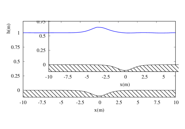
(a) Full system (3.2)

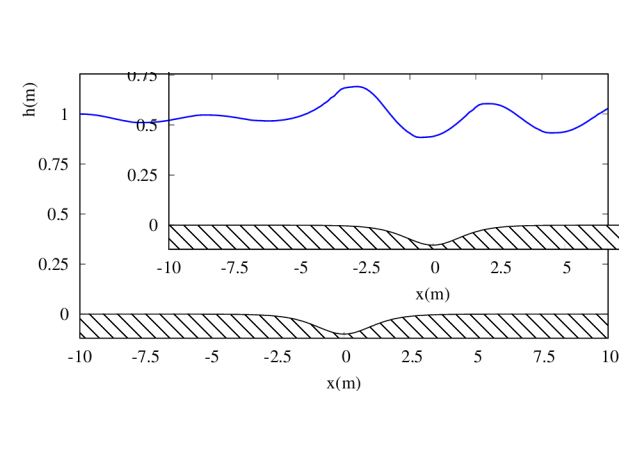
(b) Partial system (3.3) from [17]

Figure 1: Steady state solution with topography.

We show in Figure 1(a) the graph of the steady-state solution obtained numerically by solving (3.2h) (the results are shown only over the interval $(-10,10)$). The grid is composed of $200$ ${\mathbb{P}}_{1}$ elements and the final time is $t=$1000\text{\,}\mathrm{s}$$. In Figure 1(b) we show the graph of the steady-state solution obtained by solving the system (3.3) from [17]. The effects of the missing terms is clear. It would be interesting to see which of these two states can be reproduced experimentally.

4.4 1D Solitary wave propagating over a triangular obstacle

We now consider the experiments of a solitary wave propagating over a triangular obstacle described in Seabra-Santos et al. [24] and focus on the study of reflected waves. The goal here is to compare the system (3.2) to the experiments and to the incomplete model (3.3) introduced in [17]. We discover that the prediction of the amplitude of the reflected waves are exceptionally accurate when the topography corrections are fully account for. It seems that this observation and a thorough examination of the data provided in [24] for the triangular obstacle had never been done before.

In the experiments reported in [24], a reflected wave is generated when the solitary wave passes over the triangular obstacle for some values of the water depth $\mathsf{h}_{0}$ and incident wave amplitude $\alpha$. We focus on the water depths of $15\text{\,}\mathrm{c}\mathrm{m}$ and $12.5\text{\,}\mathrm{c}\mathrm{m}$ since the authors claim that the height of the reflected wave is negligible when the water depth is larger. The bathymetry in the experiments is a triangular obstacle centered at $x=$0\text{\,}\mathrm{m}$$ with a base of $14.1\text{\,}\mathrm{c}\mathrm{m}$ and height $10\text{\,}\mathrm{c}\mathrm{m}$. This triangular obstacle can be reproduced with the function $z(x)=\max(0.1-\tfrac{10}{7.05}|x|,0)$. However, the original Serre model (2.2)–(2.3) contains terms proportional to $\Delta z({\bm{x}})$ (and $\nabla(\Delta z({\bm{x}}))$) which produce a Dirac measure and the derivative of a Dirac measure at the PDE level. We handle this difficulty by introducing a mesh-dependent smoothing of the bathymetry as follows: $z(x)=\max(0.1-\tfrac{10}{7.05}\frac{x^{2}}{\left|x\right|+d\sqrt{\mathsf{h}_{0}h}},0),$ where $h$ is the mesh-size and $\mathsf{h}_{0}$ is the water depth. The constant $d$ is chosen so that on a mesh composed of 1600 ${\mathbb{P}}_{1}$ elements, the smoothing parameter $d\sqrt{\mathsf{h}_{0}h}$ is equal to $0.075$. We have numerically verified that this smoothing procedure is consistent in the sense that the solution converges in the $L^{1}$-norm as we refine the mesh.

The computational domain is set to $D=(-$20\text{\,}\mathrm{m}$,$20\text{\,}\mathrm{m}$)$. We reproduce 9 of the experiments shown in [24, Tab. 2] for $\mathsf{h}_{0}=$15\text{\,}\mathrm{c}\mathrm{m}$$ and $\mathsf{h}_{0}=$12.5\text{\,}\mathrm{c}\mathrm{m}$$ with the values of the incident wave height $\alpha$ given in Table 2. Let $\tilde{\mathsf{h}}(x,t)$ and $\tilde{u}(x,t)$ be the water height and velocity of an solitary wave:

(4.1) $$\tilde{\mathsf{h}}(x,t)=\mathsf{h}_{0}+\frac{\alpha}{(\cosh(r(x-x_{0}-ct)))^{2}},\qquad\tilde{u}(x,t)=c\frac{\tilde{\mathsf{h}}(x,t)-\mathsf{h}_{0}}{\tilde{\mathsf{h}}(x,t)},$$

with wave speed $c=\sqrt{g(\mathsf{h}_{0}+\alpha)}$ and width $r=\sqrt{\frac{3\alpha}{4\mathsf{h}_{0}^{2}(\mathsf{h}_{0}+\alpha)}}$. To be consistent with the experimental measurements, we initiate the solitary wave at $x_{0}=-15\mathsf{h}_{0}$ with

(4.2) $$\mathsf{h}(x,0)=\text{max}\{\tilde{\mathsf{h}}(x,0)-z(x),0\},\qquad q(x,0)=\tilde{u}(x,0)\mathsf{h}(x,0).$$

Here we take $g=$9.81\text{\,}\mathrm{m}\mathrm{s}^{-2}$$. We then measure the height of the reflected wave at the location $x=-25\mathsf{h}_{0}$. We run the computations with a mesh composed of 3200 ${\mathbb{P}}_{1}$ elements with CFL 0.1 until final time $t=$10\text{\,}\mathrm{s}$$. In Table 2, we report the results of our computations for the system (3.2) and the incomplete system (3.3) (denoted by the index ${}_{\text{inc}}$). In the table, $E_{r}$ is the relative difference between the computational and experiment values (shown in [24, Tab. 2]) and is defined as $E_{r}=\frac{\alpha_{r}-\alpha_{\text{Exp}}}{\alpha_{\text{Exp}}}$ for the reflected wave. Note that the amplitude values reported in Table 2 are in centimeters so a 10% error is only $1\text{\,}\mathrm{m}\mathrm{m}$. We see in the table that we have good agreement for the full system (3.2) while the incomplete system (3.3) gives very poor agreement by largely overshooting the reflected wave amplitudes.

Exp.	$\mathsf{h}_{0}$	$\alpha$	$\alpha_{r}$	$E_{r}$	$\alpha_{\text{inc},r}$	$E_{\text{inc},r}$
72	15.0	2.96	0.37	-9.8%	0.61	49%
73	15.0	4.35	0.53	-12%	1.07	78%
74	15.0	5.81	0.70	7.7%	1.64	150%
75	15.0	6.56	0.79	-1.3%	1.93	140%
76	15.0	8.40	0.96	-20%	2.56	110%
77	12.5	2.50	0.49	-18%	0.75	25%
78	12.5	4.75	0.86	7.5%	1.66	110%
79	12.5	6.0	1.03	8.4%	2.21	130%
80	12.5	6.3	1.07	1.9%	2.34	120%

Table 2: Numerical results for the passing of a solitary wave over a triangular obstacle (reflected waves). $\mathsf{h}_{0}$ is the still water depth; $\alpha$ is the amplitude of the incident wave; $\alpha_{r}$ is the amplitude of the reflected wave; $\alpha_{\text{inc},r}$ is the amplitude of the reflected wave for incomplete system (3.3). All values are in $\text{\,}\mathrm{c}\mathrm{m}$.

In Figures 2(a) and 2(b), we show the graph of the free surface $\mathsf{h}+z$ in the $(x,t)$-plane for Experiment 78 listed in Table 2 (the left panel shows the results for the full system (3.2); the right panel shows the results for the incomplete system (3.3)). The effects of the missing terms are evident: we see that the incomplete system (3.3) generates more and higher reflected waves, some of which are likely unphysical. Likewise, the incomplete system creates a wave of large amplitude when passing over the triangular peak, which we suspect is unphysical.

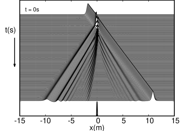
(a) $(x,t)$-plane representation of $\mathsf{h}+z$ for the relaxed system (3.2).

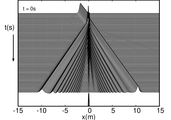
(b) $(x,t)$-plane representation of $\mathsf{h}+z$ for the incomplete, relaxed (3.3).

Figure 2: Solitary wave passing over a triangular obstacle for Exp. 78: $\mathsf{h}_{0}=$12.5\text{\,}\mathrm{c}\mathrm{m}$,\alpha=$4.75\text{\,}\mathrm{c}\mathrm{m}$$. Final time $t=$10\text{\,}\mathrm{s}$$.

4.5 1D Solitary wave propagating over a step

We now consider the problem of a solitary wave propagating over a step as described in Seabra-Santos et al. [24]. Again here we compare the numerical results to the experimental data. In particular, we focus on the fission phenomena of the solitary wave due to the passing over the step. Recall that the fission phenomena is defined to be the process by which an incident solitary wave evolves into at least two (transmitted) solitary waves ranked in order of decreasing amplitude and followed by a small dispersive tail.

The computational domain is $D=($-10\text{\,}\mathrm{m}$,$30\text{\,}\mathrm{m}$)$. The bathymetry for this problem is a step of height $0.1\text{\,}\mathrm{m}$ defined over $x\geq$0\text{\,}\mathrm{m}$$ and $0\text{\,}\mathrm{m}$ elsewhere. Similarly as in the previous section, we introduce a smoothed bathymetry profile by setting $z(x)=0.1(\frac{1}{2}+\frac{1}{\pi}\arctan(\frac{x}{d\sqrt{\mathsf{h}_{0}h}}))$ where $h$ is the mesh-size and $\mathsf{h}_{0}$ is the water depth. The constant $d$ is chosen as in the previous section. Since the computational domain is finite, we limit the reflection of waves at the left end of the domain by introducing an “absorption zone” as described in Tovar [28]. Here, the absorption zone is set to be $D_{\text{abs}}=($-10\text{\,}\mathrm{m}$,$-5\text{\,}\mathrm{m}$)$.

Exp.	$\mathsf{h}_{0}$	$\alpha$	$\alpha_{t1}$	$E_{1}$	$\alpha_{t2}$	$E_{2}$	$\alpha_{t3}$	$E_{3}$
1	30.0	4.25	5.58	13%	1.18	44%	–	–
2	30.0	6.80	8.92	4.9%	1.78	11%	–	–
3	30.0	7.10	9.30	5.1%	1.85	6.3%	–	–
4	30.0	7.50	9.81	1%	1.94	11%	–	–
6	30.0	9.70	12.54	-2.8%	2.43	2.1%	–	–
7	25.0	1.78	2.40	8.1%	0.69	-1.4%	–	–
8	25.0	2.57	3.61	15%	0.96	28%	–	–
9	25.0	3.84	5.42	14%	1.39	20%	–	–
10	25.0	5.75	7.96	-0.25%	2.03	0%	–	–
11	25.0	7.17	9.79	-5.3%	2.49	0.81%	–	–
20	20.0	1.63	2.57	8.0%	0.90	-8.2%	0.19	-57%
21	20.0	2.08	3.26	5.8%	1.17	7.3%	0.21	-25%
22	20.0	2.43	3.77	5.9%	1.36	12%	0.24	20%
23	20.0	2.93	4.49	4.4%	1.64	5.1%	0.27	-21%
24	20.0	3.65	5.48	3.2%	2.01	12%	0.32	-3%

Table 3: Numerical results for the passing of a solitary wave over a shelf (transmitted waves). $\mathsf{h}_{0}$ is the still water depth; $\alpha$ is the amplitude of the incident wave; $\alpha_{tj}$ is the amplitude of the $j$th transmitted wave. All values are in $\text{\,}\mathrm{c}\mathrm{m}$.

In the original experiments, seven wave gauges were placed along the basin to measure the wave heights, and in particular, the height of the transmitted waves. Recall that transmitted waves are waves that form after the solitary wave passes over the step and separates into multiple solitary waves (this can be seen in Figure 3). For our computations, we measure the amplitude of the transmitted waves at $x=$15\text{\,}\mathrm{m}$$ since it was stated in [24] that “a length of about 15 m was required for such a wave-sorting process”. (We note here that it’s not clear at which gauge the transmitted waves reported in [24, Tab. 1] were measured). We reproduce 15 of the experiments shown in [24, Tab. 1] and list the different values of $\mathsf{h}_{0}$ and $\alpha$ used in Table 3. The experiment numbers listed in Table 3 coincide with those of [24, Tab. 1]. We run the computations with a mesh composed of 3200 ${\mathbb{P}}_{1}$ elements with $\text{CFL}=0.1$ until the final time $t=$20\text{\,}\mathrm{s}$$ for Experiments 1-10 and $t=$25\text{\,}\mathrm{s}$$ for Experiment 20-24. In Table 3, we report the results of our computations and compare the transmitted wave heights to those reported in [24]. In the table, $E_{j}$ is the relative difference between the computational and experiment values and is defined as $E_{j}=\frac{\alpha_{j}-\alpha_{\text{Exp}}}{\alpha_{\text{Exp}}}$ for each $j$-th transmitted wave. Good agreement with the experimental data is observed overall. In Figure 3, we show the graph of the free surface $\mathsf{h}+z$ in the $(x,t)$-plane for Experiment 10 and 24 listed in Table 3.

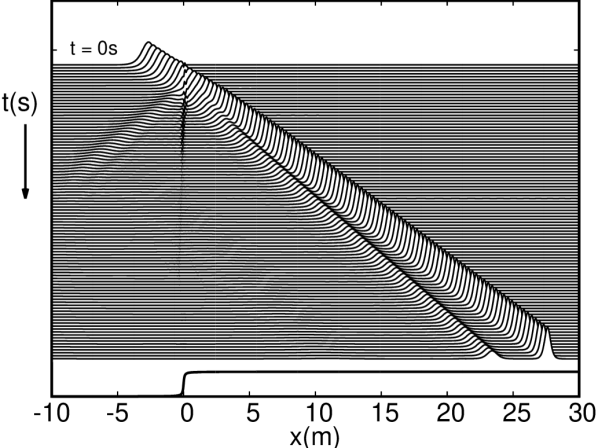
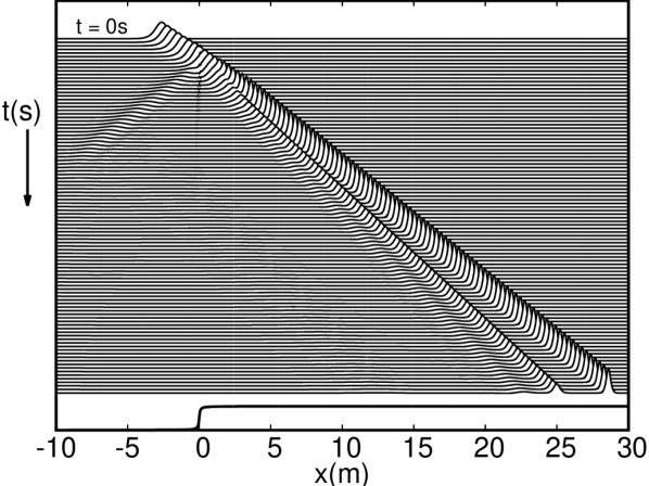
Figure 3: Time evolution plot of a solitary wave propagating over a discontinuous step for Exp. 10 and Exp. 24. Final time $t=$20\text{\,}\mathrm{s}$$ and $t=$25\text{\,}\mathrm{s}$$, respectively.

4.6 1D Shoaling of solitary waves over sloped beach

We now consider the 1994 experiments of Guibourg [18] conducted at LEGI (Laboratoire des Écoulements Géophysiques et Industriels) in Grenoble, France, to investigate the shoaling of solitary waves over a sloped beach.

We consider 4 series of experiments proposed in [18] with a reference water depth of $\mathsf{h}_{0}=$0.25\text{\,}\mathrm{m}$$ and different solitary wave amplitudes (see: Table 4). We simulate the experiments in one spatial dimension and reproduce the bathymetry as follows:

$$z(x)=\begin{cases}\frac{1}{30}(x-2.5)-\mathsf{h}_{0},&x\geq 25\\ -\mathsf{h}_{0},&\text{otherwise}.\end{cases}$$

	Case 1	Case 2	Case 3	Case 4
$\alpha/\mathsf{h}_{0}$	0.096	0.2975	0.456	0.5343
WG1	$7.75\text{\,}\mathrm{m}$	$5.75\text{\,}\mathrm{m}$	$4.25\text{\,}\mathrm{m}$	$4.25\text{\,}\mathrm{m}$
WG2	$8.25\text{\,}\mathrm{m}$	$6.25\text{\,}\mathrm{m}$	$5.0\text{\,}\mathrm{m}$	$5.0\text{\,}\mathrm{m}$
WG3	$8.75\text{\,}\mathrm{m}$	$6.75\text{\,}\mathrm{m}$	$5.75\text{\,}\mathrm{m}$	$5.75\text{\,}\mathrm{m}$

Table 4: Solitary wave shoaling experiment [18] – configuaration values

The computational domain is set to $D=($-5\text{\,}\mathrm{m}$,$35\text{\,}\mathrm{m}$)$. For each experiment, we initialize the solitary wave at $x_{0}=$0\text{\,}\mathrm{m}$$ with the profiles defined in (4.2) and the amplitudes shown in Table 4. We run the computations to the final time $T=$10\text{\,}\mathrm{s}$$ on the three difference meshes with respective mesh-size: $h=\{$0.05\text{\,}\mathrm{m}$,$0.025\text{\,}\mathrm{m}$,$0.0125\text{\,}\mathrm{m}$\}$ (corresponding to $800,1600,3200$ ${\mathbb{P}}_{1}$ elements). The CFL number is set to $0.1$. We set wall boundary conditions at both ends of the domain.

In the experiments, the wave elevation was measured with three wave gauges (WGs) which were moved for each case. We report the location of the wave gauges in Table 4. In Figure 4, we show the comparisons with the numerical computations and the experimental data for each case. We observe that the numerical results match the experimental data reasonably well. This set of experiments reinforces the observations made in §4.4 and §4.5 that the dispersive Serre model with topography effects captures well the shoaling phenomenon induced by topography.

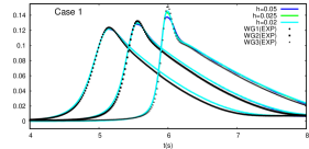
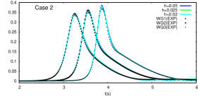
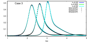
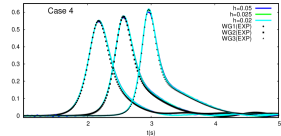
Figure 4: Comparison of numerical results with experimental data for solitary wave shoaling experiments of [18].

4.7 1D Periodic waves propagation over a submerged bar

We now consider the 1994 experiments conducted in Beji and Battjes [4] which investigate the propagation of periodic waves over a submerged trapezoidal bar. The goal of the experiments is to model the interaction of highly dispersive waves, and in particular, the release of higher-harmonics into a deeper region after the shoaling process.

We consider two of the experimental setups described in [4]: (i) sinusoidal long waves (SL) with target amplitude $a=$1\text{\,}\mathrm{c}\mathrm{m}$$ and period $T_{p}=$2\text{\,}\mathrm{s}$$; (ii) sinusoidal high-frequency waves (SH) with target amplitude $a=$1\text{\,}\mathrm{c}\mathrm{m}$$ and period $T_{p}=$1.25\text{\,}\mathrm{s}$$. We simulate these experiments in one spatial dimension and reproduce the bathymetry of the submerged bar as follows:

$$z(x)=\begin{cases}\frac{1}{20}(x-6),&6\leq x\leq 12\\ 0.3,&12\leq x\leq 14\\ 0.3-\frac{1}{10}(x-14),&14\leq x\leq 17\\ 0,&\text{otherwise}.\end{cases}$$

Figure 5: Submerged bar set up with gauge locations.

The computational domain is set to be $D=(-$12.3\text{\,}\mathrm{m}$,$37.7\text{\,}\mathrm{m}$)$. We impose two relaxation zones in the domain for the generation and absorption of waves (we refer the reader to Tovar [28] for the details). The length of the generation zone for the SL case is $6\text{\,}\mathrm{m}$ (approximately 1.5 wavelengths) and $4\text{\,}\mathrm{m}$ for the SH case (approximately 2.0 wavelengths). The absorption zone for both cases is set to $D_{\text{abs}}=($25\text{\,}\mathrm{m}$,$37.7\text{\,}\mathrm{m}$)$. We set the reference water depth to ${\mathsf{H}}_{0}=$0.4\text{\,}\mathrm{m}$$ and initialize the water height profile with $\mathsf{h}_{0}(x)={\mathsf{H}}_{0}-z({\bm{x}})$ and discharge $q_{0}(x)=0$. The periodic waves are introduced into the domain via the generation zone with the profiles given by:

$$\mathsf{h}(x,t)=\mathsf{h}_{0}+a\sin(kx-\sigma t),\quad u(x,t)=\frac{a}{\mathsf{h}_{0}}\frac{\sigma}{k}\sin(kx-\sigma t),$$

where $a$ is the amplitude, $k$ the wave number and $\sigma$ the wave frequency. Here, we define the wave frequency by $\sigma=\tfrac{2\pi}{T_{p}}$ and $k$ is found by using the dispersion relation for the full Serre model: $k^{2}=3\sigma^{2}/(3g\mathsf{h}_{0}-\mathsf{h}_{0}^{2}\sigma^{2})$. We set the final time to be $t=$60\text{\,}\mathrm{s}$$ and run with CFL=0.175. We run the computations on three different meshes with mesh-size $h=\{$0.05\text{\,}\mathrm{m}$,$0.025\text{\,}\mathrm{m}$,$0.0125\text{\,}\mathrm{m}$\}$ (corresponding to $1000$, $2000$, and $4000$ ${\mathbb{P}}_{1}$ cells.).

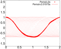
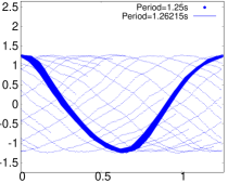
Figure 6: Illustration of period-folding with experimental wave gauge 1 with SL case (left) and SH case (right).

In the original experiments, seven wave gauges (WGs) were used to measure the water elevation: WG1($x=$5.7\text{\,}\mathrm{m}$$), WG2($x=$10.5\text{\,}\mathrm{m}$$), WG3($x=$12.5\text{\,}\mathrm{m}$$), WG4($x=$13.5\text{\,}\mathrm{m}$$), WG5($x=$14.5\text{\,}\mathrm{m}$$), WG6($x=$15.7\text{\,}\mathrm{m}$$), WG7($x=$17.3\text{\,}\mathrm{m}$$). In Figure 5, we show the locations of these wave gauges with respect to the bathymetry. The experimental data used here was obtained from the original author of the experiments, Serdar Beji. It was our experience that the experimental data did not quite match the targeted values of the period mentioned above. To illustrate this, we introduce a post-processing technique of the experimental data that we call period-folding. The idea is that given some experimental time series that is supposedly periodic with period $T_{p}$ in the time interval $[t_{0},T_{\text{final}}]$, the folding of the sequence obtained by the mapping $t\mapsto t-t_{0}-\lfloor\frac{t-t_{0}}{T_{p}}\rfloor T_{p}$ should represent the evolution of the signal during one period (here $\lfloor{\cdot}\rfloor$ is the floor function). Doing this folding gives a better idea of the long time behavior of the experimental data than just looking at one specific window of length $T_{p}$ as often done in the literature. In particular it reveals whether the signal is indeed periodic with period $T_{p}$. In Figure 6, we use period folding for the experimental data at WG1 with the targeted values of $T_{p}$. This process shows that the experimental data have not exactly the alleged period. We have been able to discover a good approximation of the actual period $T_{p}^{\text{adj}}$ by doing the period folding with various values of $T_{p}$: (i) SL case, $T_{p}=$2\text{\,}\mathrm{s}$$, $T_{p}^{\text{adj}}=$2.019\,75\text{\,}\mathrm{s}$$; (ii) SH case, $T_{p}=$1.25\text{\,}\mathrm{s}$$, $T_{p}^{\text{adj}}=$1.262\,15\text{\,}\mathrm{s}$$. We also note that the wave amplitude value for the SH case is closer to $0.014\text{\,}\mathrm{m}$ and this is what we use for our computations.

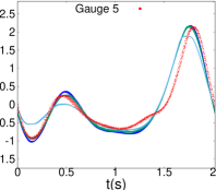
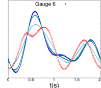
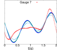
Figure 7: SL Case. Water elevation at seven gauges. Numerical results using three meshes, $h=\{$0.05\text{\,}\mathrm{m}$,$0.025\text{\,}\mathrm{m}$,$0.0125\text{\,}\mathrm{m}$\}$ (solid lines). Experimental data (red points).

Figure 8: SH Case. Water elevation at seven gauges. Numerical results using three meshes, $h=\{$0.05\text{\,}\mathrm{m}$,$0.025\text{\,}\mathrm{m}$,$0.0125\text{\,}\mathrm{m}$\}$ (solid lines). experimental data (red points).

Using the adjusted values above and the period-folding technique, we compare in Figures 7 and 8 the experimental data and the results of the computations at the wave gauges 2–7 (Figure 7 for the SL experiment and and Figure 8 for the SH experiment). For the experimental data, we choose $t_{0}$ to be the time corresponding to the second maximum wave height of the signal at WG2. For the numerical simulations, we choose $t_{0}$ to be the time corresponding to the maximum wave height around $t\approx$40\text{\,}\mathrm{s}$$ at WG2. We observe that the numerical results converge as the mesh is refined. The SH experiment is relatively well reproduced at all the gauges. There are slight deviations at the last two gauges behind the bar for the SL experiment. It is possible that some wave breaking occurs between gauges 5 and 6 in this case. We note here that the results shown above are very similar to those seen in Bassi et al. [3] in Figure 9 and Figure 10 therein.

4.8 2D Solitary wave run-up over a conical island

We consider the 1995 laboratory experiments conducted by Briggs et al. [6] at the US Army Waterways Experiment Station in Vicksburg, Mississippi (now the US Army Engineer Rsearch and Development Center). The laboratory experiments were motivated by several tsunami events in the 1990s where large unexpected run-up heights were observed on the back (or lee) side of small islands. Several authors have used this experiment to study the run-up phenomena using the classical Shallow Water model and other dispersive models (see: Hou et al. [19], Lannes and Marche [22], Kazolea et al. [20]).

Let $r({\bm{x}})$ by the radius from the center of the island located at $($12.96\text{\,}\mathrm{m}$,$13.80\text{\,}\mathrm{m}$)$. Then the conical island bathymetry is defined by

(4.3) $$z({\bm{x}})=\begin{cases}\min\left(\mathsf{h}_{\text{top}},\mathsf{h}_{\text{cone}}-r({\bm{x}})/s_{\text{cone}}\right),&r({\bm{x}})<r_{\text{cone}}\\ 0,&\text{otherwise}\end{cases},$$

where $\mathsf{h}_{\text{top}}=0.625$\mathrm{m}$,\mathsf{h}_{\text{cone}}=0.9$\mathrm{m}$$ and $r_{\text{cone}}=3.6$\mathrm{m}$$. We reproduce two experiments, which we call Case B and Case C, with $\alpha/\mathsf{h}_{0}=0.091$ and $\alpha/\mathsf{h}_{0}=0.181$ where $\mathsf{h}_{0}=$0.32\text{\,}\mathrm{m}$$ and $\alpha$ is the amplitude of the solitary wave.

The computations are done in the domain $(0,$25\text{\,}\mathrm{m}$)\times(0,$30\text{\,}\mathrm{m}$)$ until the final time $T=$12\text{\,}\mathrm{s}$$ with wall boundary conditions and CFL number 0.25. We initiate the solitary wave at $x_{0}=9.36-\frac{L}{2}$ using (4.1) with $L=\frac{2\mathsf{h}_{0}}{k}\operatorname{arccosh}\sqrt{20}$ and $k=\sqrt{\frac{3\alpha}{4\mathsf{h}_{0}}}$. Here $x_{0}$ is the location of the experimental wave gauge 3 (WG3) which was used to measure the free surface elevation away from the island. In Figure 9, we show the surface plots of the free surface elevation $\mathsf{h}+z$ on a mesh composed of 52,129 $\boldsymbol{\mathbb{P}}_{1}$ nodes at $t=\{0,5.8,$8\text{\,}\mathrm{s}$\}$.

Figure 9: Experiment 4 – Surface plot of the water elevation $\mathsf{h}+z$ at several times for Case C. The thin grey cylinders represent the wave gauges WG3, WG6, WG9, WG16, WG22 (left to right).

In the experiment, several wave gauges were placed around the island to measure the free surface elevation and wave run-up. We compare the numerical results with the measurents at four of the experimental wave gauges: WG6$($9.36\text{\,}\mathrm{m}$,$13.80\text{\,}\mathrm{m}$)$, WG9$($10.36\text{\,}\mathrm{m}$,$13.80\text{\,}\mathrm{m}$)$, WG16$($12.96\text{\,}\mathrm{m}$,$11.22\text{\,}\mathrm{m}$)$, WG22$($15.56\text{\,}\mathrm{m}$,$13.80\text{\,}\mathrm{m}$)$. In Figure 10, we show the comparison with the experimental data and numerical simulations for both Case B (on the left) and Case C (on the right). For both cases, the numerical results show good agreement with the experimental data. We capture well the magnitudes of the run-up and draw-down at the front side of the island at WG9 with a slight overshoot in Case C. For both cases, we see very good comparison with WG16 which corresponds to the run-up and draw-down on the side of the island. We note that the experimental data shows subsequent free surface oscillations after impacting the island which is most notable in WG9, but our numerical simulation do not capture this effect. This phenomena is consistent with the literature and has been observed by others (see: Lannes and Marche [22], Kazolea et al. [20], Yamazaki et al. [29]), and is likely due to inconsistency in the original experiments.

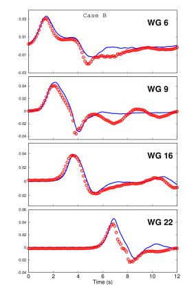
Figure 10: Experiment 4 – Temporal series over the period $t\in[0,$12\text{\,}\mathrm{s}$]$ of the free surface elvation $\mathsf{h}+z$ in meters at the four WGs (blue solid) compared to the experimental data (red circles) for Case B (on the left) and Case C (on the right).

5 Conclusion

In this paper we introduced a relaxation technique for solving the dispersive Serre equations with full effects induced by the topography. We also derived a family of analytical solutions to the dispersive Serre equations that can be used for validating numerical methods. The relaxation approach yields a new hyperbolic system that is compatible with dry states and extends the work presented in [17]. This hyperbolic system is then shown numerically to converge to the original dispersive Serre model at the expected first-order convergence rate when the relaxation parameter is chosen to be proportional to the local mesh-size. We then compared our numerical computations with several laboratory experiments for model validation and demonstrated close agreement with said data. We also showed that neglecting the full terms induced by the topography as was done in [17] yields poor agreement with the experimental data and thus shows the importance of these terms.

References

- Alvarez-Samaniego and Lannes [2008] B. Alvarez-Samaniego and D. Lannes. Large time existence for 3D water-waves and asymptotics. Invent. Math., 171(3):485–541, 2008.
- Barthélemy [2004] E. Barthélemy. Nonlinear shallow water theories for coastal waves. Surveys in Geophysics, 25:315–337, 2004.
- Bassi et al. [2020] C. Bassi, L. Bonaventura, S. Busto, and M. Dumbser. A hyperbolic reformulation of the Serre–Green–Naghdi model for general bottom topographies. Computers & Fluids, 212:104716, 2020.
- Beji and Battjes [1994] S. Beji and J. Battjes. Numerical simulation of nonlinear wave propagation over a bar. Coastal Engineering, 23(1):1 – 16, 1994.
- Bonneton et al. [2011] P. Bonneton, F. Chazel, D. Lannes, F. Marche, and M. Tissier. A splitting approach for the fully nonlinear and weakly dispersive Green–Naghdi model. J. Comput. Phys., 230(4):1479–1498, 2011.
- Briggs et al. [1995] M. J. Briggs, C. E. Synolakis, G. S. Harkins, and D. R. Green. Laboratory experiments of tsunami runup on a circular island. pure and applied geophysics, 144(3):569–593, 1995.
- Bristeau et al. [2015] M.-O. Bristeau, A. Mangeney, J. Sainte-Marie, and N. Seguin. An energy-consistent depth-averaged Euler system: derivation and properties. Discrete Contin. Dyn. Syst. Ser. B, 20(4):961–988, 2015.
- Castro and Lannes [2014] A. Castro and D. Lannes. Fully nonlinear long-wave models in the presence of vorticity. Journal of Fluid Mechanics, 759:642–675, 2014.
- Duran and Marche [2017] A. Duran and F. Marche. A discontinuous Galerkin method for a new class of Green–Naghdi equations on simplicial unstructured meshes. Appl. Math. Model., 45:840–864, 2017.
- Escalante et al. [2019] C. Escalante, M. Dumbser, and M. J. Castro. An efficient hyperbolic relaxation system for dispersive non-hydrostatic water waves and its solution with high order discontinuous Galerkin schemes. J. Comput. Phys., 394:385–416, 2019.
- Favrie and Gavrilyuk [2017] N. Favrie and S. Gavrilyuk. A rapid numerical method for solving Serre–Green–Naghdi equations describing long free surface gravity waves. Nonlinearity, 30(7):2718–2736, 2017.
- Fernandez-Nieto et al. [2019] E. D. Fernandez-Nieto, M. Parisot, Y. Penel, and J. Sainte-Marie. A hierarchy of dispersive layer-averaged approximations of euler equations for free surface flows. Communications in Mathematical Sciences, 16(5):1169–1202, 2019.
- Gavrilyuk and Shugrin [1996] S. L. Gavrilyuk and S. M. Shugrin. Media with equations of state that depend on derivatives. Journal of Applied Mechanics and Technical Physics, 37(2):177–189, 1996.
- Green and Naghdi [1976] A. E. Green and P. M. Naghdi. A derivation of equations for wave propagation in water of variable depth. Journal of Fluid Mechanics, 78(2):237–246, 1976. 10.1017/S0022112076002425.
- Green et al. [1974] A. E. Green, N. Laws, and P. M. Naghdi. On the theory of water waves. Proc. Roy. Soc. (London) Ser. A, 338:43–55, 1974.
- Guermond et al. [2018] J.-L. Guermond, M. Quezada de Luna, B. Popov, C. Kees, and M. Farthing. Well-balanced second-order finite element approximation of the shallow water equations with friction. SIAM Journal on Scientific Computing, 40(6):A3873–A3901, 2018.
- Guermond et al. [2019] J.-L. Guermond, B. Popov, E. Tovar, and C. Kees. Robust explicit relaxation technique for solving the Green–Naghdi equations. J. Comput. Phys., 399:108917, 17, 2019.
- Guibourg [1994] S. Guibourg. Modélisations numérique et expérimentale des houles bidimensionnelles en zone cotière. PhD thesis, 1994. URL http://www.theses.fr/1994GRE10160.
- Hou et al. [2013] J. Hou, Q. Liang, F. Simons, and R. Hinkelmann. A stable 2d unstructured shallow flow model for simulations of wetting and drying over rough terrains. Computers & Fluids, 82:132 – 147, 2013.
- Kazolea et al. [2012] M. Kazolea, A. Delis, I. Nikolos, and C. Synolakis. An unstructured finite volume numerical scheme for extended 2d boussinesq-type equations. Coastal Engineering, 69:42 – 66, 2012.
- Lannes [2020] D. Lannes. Modeling shallow water waves. Nonlinearity, 33(5):R1–R57, 2020.
- Lannes and Marche [2015] D. Lannes and F. Marche. A new class of fully nonlinear and weakly dispersive Green–Naghdi models for efficient 2d simulations. Journal of Computational Physics, 282:238 – 268, 2015.
- Samii and Dawson [2018] A. Samii and C. Dawson. An explicit hybridized discontinuous galerkin method for Serre–Green–Naghdi wave model. Computer Methods in Applied Mechanics and Engineering, 330:447 – 470, 2018.
- Seabra-Santos et al. [1987] F. J. Seabra-Santos, D. P. Renouard, and A. M. Temperville. Numerical and experimental study of the transformation of a solitary wave over a shelf or isolated obstacle. Journal of Fluid Mechanics, 176:117–134, 1987.
- Serre [1953] F. Serre. Contribution à l’étude des écoulements permanents et variables dans les canaux. La Houille Blanche, (6):830–872, 1953. URL https://doi.org/10.1051/lhb/1953058.
- Su and Gardner [1969] C. H. Su and C. S. Gardner. Korteweg-de Vries equation and generalizations. III. Derivation of the Korteweg-de Vries equation and Burgers equation. J. Mathematical Phys., 10:536–539, 1969.
- Tkachenko [2020] S. Tkachenko. Analytical and numerical study of a dispersive shallow water model. PhD thesis, Aix-Marseille University, 2020.
- Tovar [2021] E. Tovar. Well-balanced and invariant domain preserving schemes for dispersive shallow water flows. PhD thesis, Texas A&M, 2021. In preparation.
- Yamazaki et al. [2009] Y. Yamazaki, Z. Kowalik, and K. F. Cheung. Depth-integrated, non-hydrostatic model for wave breaking and run-up. International Journal for Numerical Methods in Fluids, 61(5):473–497, 2009.