KANAZAWA-21-01

June, 2021

Sommerfeld-enhanced dark matter searches with dwarf spheroidal galaxies

Shin’ichiro Ando^(a,b), Koji Ishiwata^(c)

^(a)GRAPPA Institute, University of Amsterdam, 1098 XH Amsterdam,
The Netherlands

^(b)Kavli Institute for the Physics and Mathematics of the Universe (Kavli IPMU, WPI), University of Tokyo, Kashiwa, Chiba 277-8583, Japan

^(c)Institute for Theoretical Physics, Kanazawa University, Kanazawa 920-1192, Japan

1 Introduction

What dark matter (DM) is made of is one of the greatest mysteries in contemporary particle physics, astrophysics, and cosmology. Although its nature, such as mass and interaction with other particles, is unknown, weakly interacting massive particles (WIMPs) are one of the most popular DM candidates. In the WIMP hypothesis, the current abundance of DM measured by the Planck Collaboration [1] is explained by the thermal freeze-out scenario in the early Universe. This means that the WIMP DM possibly annihilates into the standard-model (SM) particles, which may be detected as high-energy messengers such as gamma rays on the Earth.

While lots of particle physics models for WIMP candidates are proposed to account for DM, Wino or Higgsino is one of the well-motivated candidates among them. They are superpartners of the $W$ and Higgs bosons in supersymmetric models. Motivated by the results of the Large Hadron Collider, supersymmetric models where supersymmetry breaks at very-high-energy scales have been revisited as an attractive framework up to the grand unification scale. Split supersymmetry [2, 3, 4, 5], high-scale supersymmetry [6], spread supersymmetry [7], and pure gravity mediation [8, 9] are the examples. In the high-scale supersymmetry, pure Wino or pure Higgsino is the DM candidate. Due to their pure nature, they interact with the SM particles via the gauge interactions. As a consequence, their scattering or annihilation cross sections are in principle determined with small theoretical uncertainties for a given mass. The scattering cross section of the Wino or Higgsino with nucleons can be determined at the next-to-leading order level of quantum chromodynamics in a consistent manner [10]. On the other hand, the annihilation process is associated with the so-called Sommerfeld enhancement that leads to non-trivial behavior of the annihilation cross section as a function of mass [20, 21, 22]. As a consequence, 2.7–3.0 TeV mass is predicted to yield the right relic abundance of the Wino as DM [22] (See Ref. [23] for recent developments.) The Sommerfeld effect is an issue not just for the Wino or Higgsino, but it can happen for DM candidates that, for example, interact with a light mediator via a Yukawa interaction (see Ref. [24] for a review). For such DM candidates, accurate predictions of Sommerfeld-enhanced signals is important in order to detect DM indirectly using high-energy gamma rays and other cosmic messengers.

Detecting gamma rays from dwarf spheroidal galaxies (dSphs) is one of the most promising avenues in the indirect DM searches. While dSphs have abundant DM component, they contain less baryonic matter compared with other galaxies. Consequently, they are an ideal object in order to detect gamma-ray signals from DM with small astrophysical backgrounds. Recently, lots of new ultrafaint dSphs have been discovered [25]. Since they are faint with much less amount of baryons, they might be more suitable for the DM searches. This fact, however, makes it difficult to determine density profiles of the ultrafaint dSphs due to the lack of stellar kinematics data.

A Bayesian approach is often adopted for estimations of density profile parameters. Representative examples are a scale radius $r_{s}$ and a characteristic mass density $\rho_{s}$ of the often adopted Navarro-Frenk-White (NFW) profile [26]. The Bayesian approach has to adopt the prior distribution of these parameters, which are combined with the likelihood to obtain the posterior probability distribution function. While uninformative, uniform priors for both $\log r_{s}$ and $\log\rho_{s}$ are usually adopted in the literature (e.g., [27]), more realistic priors based on theories of the structure formation, called satellite priors, are proposed [28]. The authors showed substantial impact on DM searches using dSphs. As a result of adopting the satellite priors, the constraints on the annihilation cross section for 10-1000 GeV DM are found to be relaxed by a factor of 2–7 compared with those obtained with uninformative, log-uniform priors [29]. It is therefore crucial to adopt more realistic priors that take into account the observed satellite dynamics in order to constrain the DM cross section.

In this work, we extend the approach of Ref. [28] and adopt the satellite priors to predict the rates of WIMP DM annihilation that is enhanced by the Sommerfeld effect. To see the impact of the satellite priors on the observable signatures, we study two Majorana DM models: (1) a model with a light scalar mediator and (2) the Wino DM in supersymmetric scenarios with masses around 3 TeV. In the former model, Refs. [30, 31, 33, 32] have already done intensive analysis, but using uninformative flat priors. Since the annihilation cross section, $\sigma v$, in this case has velocity dependence, one has to take the internal velocity structure of the dSphs into account. The models developed in Ref. [28] specify the internal density structure of each given dSph, from which we can compute the velocity distribution function (or the phase-space density of DM in the dSph). We find, for the first time, that in comparison with the case of uninformative priors, adopting the informative satellite priors decreases the expected annihilation rate by a factor of 2.7 and 1.4 using models with $V_{50}=10.5$ km s^-1 and 18 km s^-1, respectively, where $V_{50}$ is a parameter corresponding to the threshold of the maximum circular velocity of the subhalo above which satellite galaxies are assumed to form (see Sec. 2 for more details), for one of the most promising ultrafaint dSphs, Reticulum II. In addition, we find that those factors are almost independent of a parameter $\epsilon_{\phi}$ defined later in Eq. (3), i.e., ratio of DM mass and a mediator mass times the coupling that mediates the DM annihilation, except for a region where the annihilation is enhanced significantly.

For the latter Wino model, the Galactic center would be the most promising object to detect gamma rays from the DM annihilation [35, 34]. On the other hand, dSphs are also considered to be one of the most important targets for the DM search with the Cherenkov Telescope Array (CTA) observatory [38, 39]. Yet, as far as we are aware, no dedicated study on the CTA sensitivity estimates for the Wino DM searches has been performed. We, therefore, show sensitivity projection for the CTA North for several classical and ultrafaint dSphs. Even though the velocity dependence can be safely ignored for the Wino masses much heavier than the gauge boson mass, the resultant J factor changes, for example, by a factor of 1.8 between adopting priors with $V_{50}=18$ km s^-1 and $10.5$ km s^-1 for Reticulum II. Eventually it is found that both classical and ultrafaint dSphs are promising targets to detect the Wino DM with 2.7–3 TeV masses, providing a complementary method to the observation of the Galactic center.

Lastly, we note that we made the codes to generate the satellite prior distributions of $r_{s}$, $\rho_{s}$, etc., for any of both the classical and ultrafaint dSphs that are discussed in this paper publicly available at https://github.com/shinichiroando/dwarf_params.

The rest of the paper is organized as follows. In Sec. 2, we summarize the satellite priors and how to determine probability distribution of the profile parameters. Section 3 introduces formulae to compute J-factor and shows the numerical results of the light mediator model and the Wino DM. Current constraints and future sensitivity by the CTA collaboration are discussed in Sec. 4, and we conclude the paper in Sec. 5.

2 Analysis with satellite priors

In our study, we perform the analysis by using satellite priors, which we briefly summarize in this section. See Refs. [28, 40] for more details.

We use prior probability distribution function (PDF) for the subhalo parameters and the observed parameters of dSphs to give the posterior PDF for the satellite parameters. Here is a list of quantities involved in the PDF:

• subhalo parameters: ${\bf\it\theta}=(\rho_{s},r_{s},r_{t})$;

• observed dSphs data: ${\bf\it d}=(\theta_{h},\sigma_{\rm los},D)$.

Here, $r_{t}$ is the truncation radius, and $\theta_{h}$, $\sigma_{\rm los}$ and $D$ are the projected angular half-light radius, line-of-sight velocity dispersion and the distance, respectively. In our study, we adopt the NFW profile for the DM density,

$$\rho(r)=\frac{\rho_{s}}{(r/r_{s})(1+r/r_{s})^{2}}\,.$$ (1)

The prior PDF for the subhalo parameters ${\bf\it\theta}$ is proportional to the number of subhalos per volume in the parameter space $d{\bf\it\theta}$, i.e.,

$$P_{\rm sh}({\bf\it\theta})\propto\frac{d^{3}N_{\rm sh}}{d\rho_{s}dr_{s}dr_{t}}\,.$$ (2)

We note that not all of subhalos host satellite galaxies. To take the satellite formation into account, we adopt a prescription provided in Ref. [41]. We parameterize the probability that a satellite galaxy is formed in a host subhalo as

$$P_{\rm form}(V_{{\rm peak}})=\frac{1}{2}\left[1+{\rm erf}\left(\frac{V_{{\rm peak}}-V_{50}}{\sqrt{2}\sigma}\right)\right]\,,$$ (3)

where $V_{{\rm peak}}$ is the peak value of the maximum circular velocity of the subhalo. In our model, it is given as the maximum circular velocity at the subhalo accretion onto its host, $V_{\rm peak}=V_{{\rm max},a}=r_{s,a}(4\pi G\rho_{s,a}/4.625)^{1/2}$, where $G$ is the Newtonian constant of gravity and the subscript $a$ represents quantities at the time of accretion. $V_{50}$ is another input parameter. If $V_{\rm peak}$ exceeds $V_{50}$, then a satellite galaxy is formed in a host subhalo. $V_{50}=18$ km s^-1 is a value according to the conventional theory of galaxy formation. On the other hand, Ref. [41] suggests $V_{50}=10.5$ km s^-1 since $V_{50}=18$ km s^-1 underpredicts the number of dSphs and their radial distributions compared with observations. In our analysis, we adopt $V_{50}=10.5$ km s^-1 and $18$ km s^-1 for ultrafaint dSphs and $25$ km s^-1 for classical dSphs, and $\sigma=2.5$ km s^-1 based on Ref. [41]. Therefore, we construct the satellite prior PDF, $P_{\rm sat}({\bf\it\theta})$, as

$$P_{\rm sat}({\bf\it\theta})=P_{\rm sh}({\bf\it\theta})P_{\rm form}(V_{{\rm peak}})\,.$$ (4)

According to the Bayes’ theorem, the posterior PDF $P_{\rm sat}({\bf\it\theta}|{\bf\it d})$ for the subhalo parameters is given by

$$P_{\rm sat}({\bf\it\theta}|{\bf\it d})\propto P_{\rm sat}({\bf\it\theta}){\cal L}({\bf\it d}|{\bf\it\theta}),$$ (5)

where ${\cal L}({\bf\it d}|{\bf\it\theta})$ is likelihood function of obtaining data ${\bf\it d}$ for a dSph given the model parameters ${\bf\it\theta}$. The likelihood is given by

$${\cal L}({\bf\it d}|{\bf\it\theta})=\prod_{x=\{\theta_{h},\sigma_{\rm los},D\}}\frac{1}{\sqrt{2\pi\sigma_{x}^{2}}}\exp\left[-\frac{(x-x_{\rm obs})^{2}}{2\sigma_{x}^{2}}\right]\,,$$ (6)

where $x_{\rm obs}$ is the central value of the observation and $\sigma_{x}$ is the measurement uncertainty of $x$. For these values, we use the results summarized in Tables I and II of Ref. [28].

$P_{\rm sh}({\bf\it\theta})$ is obtained as follows. The input parameters are $(z_{a},m_{a},c_{{\rm vir},a})$, where $m_{a}$ is the mass of a halo that accreted onto its host halo and $z_{a}$ is the redshift at the accretion. $c_{{\rm vir},a}$ is the virial concentration parameter at the accretion, for which we adopt log-normal distribution with standard deviation $\sigma_{\log c}=0.13$ [42] while its mean value is obtained by Ref. [43]. From a set of the input parameters, characteristic radius $r_{s,a}$ and density $\rho_{s,a}$ at the accretion are obtained. In general $(r_{s}(z)$, $\rho_{s}(z))$ at redshift $z$ are related to the maximum velocity $V_{\rm max}(z)$ and radius $r_{\rm max}(z)$. For a profile that is proportional to $r^{-1}$ in the inner region, it is studied that $V_{\rm max}(z)$ and $r_{\rm max}(z)$ are determined by the subhalo mass $m(z)$ for given initial values of $V_{\rm max}(z_{a})$, $r_{\rm max}(z_{a})$, and $m_{a}$ [44]. Therefore, once we know the evolution of $m(z)$ after accretion, we obtain $r_{s}(z)$ and $\rho_{s}(z)$ for a given redshift. After accretion, the halo loses its mass by tidal stripping that can be described by the following differential equation,

$$\frac{dm(z)}{dt}=-A\frac{m(z)}{\tau_{\rm dyn}(z)}\left[\frac{m(z)}{M(z)}\right]^{\zeta}\,,$$ (7)

where $\tau_{\rm dyn}(z)$ is the dynamical timescale [45], and $M(z)$ [46] is the host halo mass at the redshift $z$. For parameters $A$ and $\zeta$, we use the results given in Ref. [40] that agree with the results of the N-body simulation. Then, by solving Eq. (7), we obtain the subhalo parameters $(\rho_{s},r_{s},r_{t})$ at $z=0$.

The distribution of mass $m_{a}$ and redshift $z_{a}$ of a subhalo at the accretion, $dN_{\rm sh}/(dz_{a}dm_{a})$, is obtained by the extended Press-Schechter formalism [47] that is calibrated with the numerical simulations [48]. With the initial distribution, we simulate the tidal effect for each subhalo to obtain the present distribution $d^{3}N_{\rm sh}/(d\rho_{s}dr_{s}dr_{t})$.

Prior and posterior PDFs of $r_{s}$ and $\rho_{s}$ are extensively discussed and shown in Ref. [28] for each dSph and for a chosen value of $V_{50}$ parameter (see Figs. 3 and 5–10 in Supplemental Material of Ref. [28]). For each parameter set $(r_{s},\rho_{s},r_{t})$ drawn from the posterior PDFs that can be obtained using publicly available codes at https://github.com/shinichiroando/dwarf_params, one can calculate the J-factors including the Sommerfeld enhancement, which is the focus of the following section.

3 Sommerfeld-enhanced gamma-ray flux from dSphs

We formulate gamma-ray flux from dSphs in two types of Majorana fermionic DM models; the annihilation is boosted via a light scalar mediator (Sec. 3.1) and the electroweak gauge bosons especially focusing on the Wino DM (Sec. 3.2). In Sec. 3.1 we review how to compute J-factor when the annihilation cross section is velocity dependent and give numerical results of some selected dSphs suitable for the DM search that are computed by the method explained in Sec. 2

3.1 Light scalar mediator model

The Sommerfeld enhancement factor via a light scalar mediator is given by the wavefunction, which will be defined soon in Eq. (5) (see Ref. [24] for a review). The wavefunction obeys the following Schrödinger equation where the potential is given by the Yukawa type,

$$\frac{1}{m_{\rm dm}}\frac{d^{2}\psi(r)}{dr^{2}}-V(r)\psi(r)=-m_{\rm dm}v^{2}\psi(r)\,,$$ (1)

where $m_{\rm dm}$ is the mass of DM and $v$ is the velocity of each DM particle, which can be written using the relative velocity $v_{\rm rel}$ as $v=v_{\rm rel}/2$, and the potential $V(r)$ is

$$V(r)=-\alpha_{y}\frac{e^{-m_{\phi}r}}{r}\,.$$ (2)

Here $\alpha_{y}$ is the coupling constant of the interaction and $m_{\phi}$ is the mass of the scalar mediator. It is legitimate to introduce dimensionless parameters,

$$\epsilon_{v}=\frac{v}{\alpha_{y}}\,,~{}~{}~{}\epsilon_{\phi}=\frac{m_{\phi}}{\alpha_{y}m_{\rm dm}}\,,~{}~{}~{}x=\alpha_{y}m_{\rm dm}r\,,$$ (3)

to get

$$\psi^{\prime\prime}(x)+\frac{e^{-\epsilon_{\phi}x}}{x}\psi(x)=-\epsilon_{v}^{2}\psi(x)\,,$$ (4)

where $\prime$ means derivative with respect to $x$. Here we have used the same symbol for wavefunction for simplicity.

The Sommerfeld-enhancement factor is then given by solving the Schrödinger equation under the boundary condition $\psi(0)=1$ and $\psi^{\prime}(\infty)=i\epsilon_{v}\psi(\infty),$

$$S^{\phi}(v_{\rm rel};\alpha_{y},\epsilon_{\phi})=|\psi(\infty)|^{2}\,.$$ (5)

Meanwhile we can solve the equation numerically to obtain $S^{\phi}(v_{\rm rel})$, there is an approximated formula,

$$S^{\phi}_{\rm apprx}(v_{\rm rel};\alpha_{y},\epsilon_{\phi})=\frac{(\pi/\epsilon_{v})\sinh s}{\cosh s-\cos t}\,,$$ (6)

where

$$s=\frac{12\epsilon_{v}}{\pi\epsilon_{\phi}}\,,~{}~{}~{}~{}t=2\pi\sqrt{\frac{6}{\pi^{2}\epsilon_{\phi}}-\left(\frac{6\epsilon_{v}}{\pi^{2}\epsilon_{\phi}}\right)^{2}}\,.$$ (7)

For example, see Ref. [31] for a comparison between the numerical results with this approximation. As presented there, the approximated formula agrees with the numerical results at the 10% level, which is of sufficient accuracy for the purpose of our present analysis. In the following numerical analysis of the light mediator model, we will use $S^{\phi}_{\rm apprx}(v_{\rm rel};\alpha_{y},\epsilon_{\phi})$, and parameterize the total annihilation cross section as

$$\sigma v=(\sigma v)_{0}S^{\phi}_{\rm apprx}(v_{\rm rel};\alpha_{y},\epsilon_{\phi})\,.$$ (8)

Then the gamma-ray flux is given by

$$\frac{d\Phi_{\gamma}}{dE}=J(\theta)\frac{(\sigma v)_{0}}{8\pi m_{\rm dm}^{2}}\frac{dN_{\gamma}}{dE}\,,$$ (9)

where $J(\theta)$ is the J-factor which will be given below and $dN_{\gamma}/dE$ is the gamma-ray spectrum per annihilation.

When the annihilation cross section is velocity-dependent, we need to take into account that effect to give the J-factor. Here we briefly review the formulation to compute the J-factor for velocity-dependent annihilation cross section. The velocity distribution $f(v,r)$ of the DM particle at the radius $r$ is given by Eddington’s formula [49],

$$f(v,r)=\frac{1}{\sqrt{8}\pi^{2}\rho(r)}\int^{\infty}_{R({\cal E}(r,v))}dr^{\prime}\frac{P(r^{\prime})}{\sqrt{{\cal E}(r,v)-\Psi(r^{\prime})}}\,,$$ (10)

where

$${\cal E}(r,v) =-\frac{v^{2}}{2}+\Psi(r)\,,$$ (11)

$$P(r) =\frac{d\rho(r)}{dr}\frac{d^{2}\Psi(r)}{dr^{2}}\left(\frac{d\Psi(r)}{dr}\right)^{-2}-\frac{d^{2}\rho(r)}{dr^{2}}\left(\frac{d\Psi(r)}{dr}\right)^{-1}\,.$$ (12)

$\Psi(r)$ is the gravitational potential and $R(X)$ is the inverse function of $\Psi(r)$. For the NFW profile $\Psi(r)$ is given analytically as

$$\Psi(r) =4\pi G\rho_{s}r_{s}^{2}\frac{\ln(1+r/r_{s})}{r/r_{s}}\,,$$ (13)

where $\rho_{s}$ and $r_{s}$ are the parameter of the NFW profile. By definition, $f(v,r)$ satisfies,

$$\int^{\infty}_{0}dv\,4\pi v^{2}f(v,r)=1\,.$$ (14)

Using $f(v,r)$, the velocity distribution of the two-body DM state is derived in terms of the relative velocity $v_{\rm rel}$ as

$$F(v_{\rm rel},r)=\int_{0}^{1}dz\,4\pi\int_{0}^{\infty}dv_{\rm cm}v^{2}_{\rm cm}f(v_{+},r)f(v_{-},r)\,,$$ (15)

where

$$v_{\pm}=\sqrt{v_{\rm cm}^{2}+v_{\rm rel}^{2}/4\pm v_{\rm cm}v_{\rm rel}z}\,.$$ (16)

Finally the J-factor is obtained by the line of sight (l.o.s) integral,

$$J(\theta) =\int_{{\rm l.o.s.}(\theta)}d\ell\int_{0}^{\infty}dv_{\rm rel}\,4\pi v_{\rm rel}^{2}F(v_{\rm rel},r)\rho^{2}(r)S(v_{\rm rel};{\bf\it X})\,,$$ (17)

where $S(v_{\rm rel};{\bf\it X})$ is the factor that describes the velocity dependence of the annihilation cross section and ${\bf\it X}$ stands for the other parameters in a certain DM model. In the present case, $S(v_{\rm rel};{\bf\it X})=S^{\phi}_{\rm apprx}(v_{\rm rel};\alpha_{y},\epsilon_{\phi})$. On the other hand, it is a good approximation to give the line of sight integral in cylindrical coordinate with radius $R$ and height $z$, which relate to $r$ as $r^{2}=R^{2}+z^{2}$,

$$\int_{{\rm l.o.s.}(\theta)}d\ell=\frac{1}{D^{2}}\int_{0}^{D\theta}dR\int_{0}^{r_{t}}dz\,4\pi R\,,$$ (18)

Here $D$ and $\theta$ are the distance to the dSph and the maximum polar angle from the center of the dSph that will be given in the later discussion.

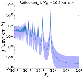
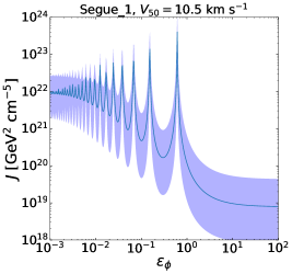
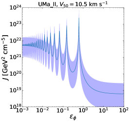
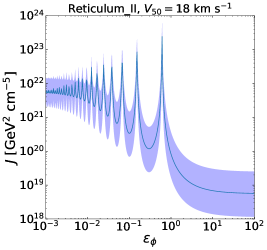
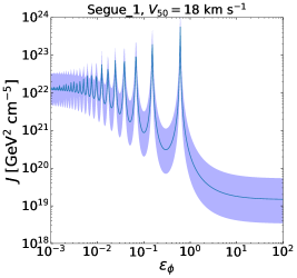
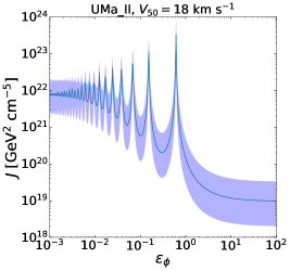
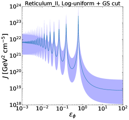
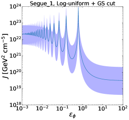
Figure 1: J-factor calculated as function of $\epsilon_{\phi}=m_{\phi}/(\alpha_{y}m_{\rm dm})$ with $\theta=0.5^{\circ}$ for ultrafaint dSphs, Reticulum II, Segue 1, and Ursa Major II (from left to right). $\alpha_{y}=10^{-2}$ and $V_{50}$ is taken to 10.5 km s^-1 (top) and 18 km s^-1 (middle). Results by using the log-uniform prior with GS15 cut [27] is plotted as a reference (bottom). Line shows the median values and shaded region corresponds to 95% credible intervals (see text for detail).

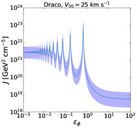
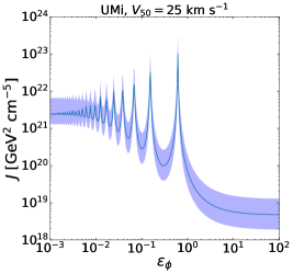
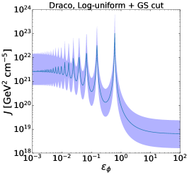
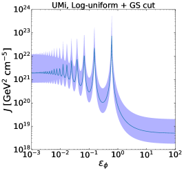
Figure 2: Same as Fig. 1 but J-factor calculated as function of $\epsilon_{\phi}$ for classical dSphs, Draco (left) and Ursa Minor (right). $V_{50}=$25 km s^-1 (top) is taken and result using log-uniform + GS cut prior is also shown (bottom).

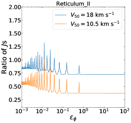
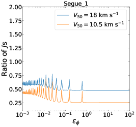
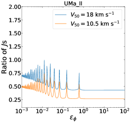
Figure 3: J-factor calculated by using $V_{50}=$10.5 km s^-1 and 18 km s^-1 that are normalized by J-factor with log-uniform prior with GS15 cut. The other parameters are the same as Fig. 1.

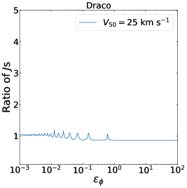
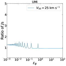
Figure 4: Same as Fig. 3 but for classical dSphs, Draco and Ursa Minor, and using $V_{50}=$25 km s^-1.

Fig. 1 shows J-factors of a few selected ultrafaint dSphs that are found to have relatively large J-factor. Here $\theta=0.5^{\circ}$ and $V_{50}=$10.5 km s^-1 (left) and 18 km s^-1 (middle) are adopted. As a comparison, the results by log-uniform priors for both $\rho_{s}$ and $r_{s}$ with abrupt cut according to cosmological argument (GS15 cut) [27] is shown for comparison (right). Shaded band shows 95% credible intervals, which are determined by the posterior distributions of the J factor for a given value of $\epsilon_{\phi}$ and $\alpha_{y}$. $\epsilon_{\phi}\to\infty$ limit corresponds to the results without the Sommerfeld enhancement that are consistent with those in Ref. [28]. It is seen that the median and credible region change in different values of $V_{50}$ for a given $\epsilon_{\phi}$. It is found that they trace the value at $\epsilon_{\phi}\to\infty$ limit; if the J-factor of a dSph for a given $V_{50}$ in this limit is larger compared to another, then the J-factor with finite $\epsilon_{\phi}$ is also larger. I.e., the differences of J-factor are nearly independent of $\epsilon_{\phi}$.

To see this explicitly, we compare J-factors computed in the prior models in Fig. 3, where J-factors using $V_{50}=10.5$ km s^-1 and $18$ km s^-1 divided by J-factor using log-uniform prior are shown. It is seen that relative value of J-factors with different priors are less sensitive to $\epsilon_{\phi}$, except for especially enhanced regions. If DM annihilation happens in the region, more precise computation might be required to determine the J-factor. Additionally, it is seen that the J factor with $V_{50}=18$ km s^-1 is larger than that with $V_{50}=10.5$ km s^-1. However, the ratio between them is differs for different dSphs. Finally, it is noted that J factor with the log-uniform prior tends to give the largest value. Since studies in the existing literature had to rely on this uninformative prior, this result shows how incorporating a more realistic, satellite prior is important to in order to determine the J factor, or the gamma-ray flux from dSphs.

For completeness, we show J-factors of some selected classical dSphs in Fig. 2, where we adopt $V_{50}=25$ km s^-1. Similarly to Fig. 3, we show the ratio of J-factors with different prior models in Fig. 4. Compared to the previous ultrafaint dSphs case, the impact of adopting the satellite prior, i.e., the choice of $V_{50}$, is small for both the Draco and Ursa Minor, as their density profiles are well determined by rich kinematics data that lead to the constraining likelihood functions. We also investigated another classical dSph, Sagittarius [50], which indeed yielded the largest J-factor, particularly because of its proximity. However, it is a system that is far from thermal equilibrium because of tidal heating and disk shocking, and our assumptions made in this study may not apply. Therefore, even though we find that our satellite priors greatly help determine the J-factor of Sagittarius by reducing associated errors, we do not discuss it any further in this study. More accurate determination of J-factors using the proper priors is important for hunting DM using dSphs, which will be discussed in Sec. 4.

3.2 Wino dark matter model

Wino is the superpartner of $W$ boson. It is $SU(2)_{L}$ triplet with hypercharge zero. Since the triplet consists of neutral and charged states, we need to solve two-component Schrödinger equation,

$$\frac{1}{m_{\rm dm}}\frac{d^{2}\psi_{i}(r)}{dr^{2}}-V_{ij}(r)\psi_{j}(r)=-m_{\rm dm}v^{2}\psi_{i}(r)\,,$$ (19)

where

$$V_{ij}(r)=\left(\begin{array}[]{cc}0&-\sqrt{2}\alpha_{W}\frac{e^{-m_{W}r}}{r}\\ -\sqrt{2}\alpha_{W}\frac{e^{-m_{W}r}}{r}{}{}{}&2\delta m-\frac{\alpha}{r}-\alpha_{W}c_{W}^{2}\frac{e^{-m_{Z}r}}{r}\end{array}\right)\,.$$ (22)

Here $\alpha$ is the fine-structure constant, $\alpha_{W}=g_{2}^{2}/(4\pi)$ ($g_{2}$ is the gauge coupling constant of $SU(2)_{L}$), $c_{W}=\cos\theta_{W}$ ($\theta_{W}$ is the Weinberg angle), and $m_{W}$ and $m_{Z}$ are the masses of $W$ and $Z$ bosons, respectively. $\delta m$ is the mass difference between charged Wino and neutral Wino. In our study, we adopt $\delta m=0.1645$ GeV [51]. As in the previous case, we introduce dimensionless parameters,

$$\epsilon_{v}=\frac{v}{\alpha_{W}}\,,~{}~{}~{}\epsilon_{W,Z}=\frac{m_{W,Z}}{\alpha_{W}m_{\rm dm}}\,,~{}~{}~{}x=\alpha_{W}m_{\rm dm}r\,,$$ (23)

to obtain,

$$\psi^{\prime\prime}_{i}(x)+\tilde{V}_{ij}(x)\psi_{j}(x)=-\epsilon_{v}^{2}\psi_{i}(x)\,,$$ (24)

where $\prime$ means derivative with respect to $x$ and

$$\tilde{V}_{ij}(x)=\frac{V_{ij}(r)}{\alpha_{W}^{2}m_{\rm dm}}=\left(\begin{array}[]{cc}0&-\sqrt{2}\frac{e^{-\epsilon_{W}x}}{x}\\ -\sqrt{2}\frac{e^{-\epsilon_{W}x}}{x}{}{}{}&\frac{2\delta m}{\alpha_{W}^{2}m_{\rm dm}}-\frac{s_{W}^{2}}{x}-c_{W}^{2}\frac{e^{-\epsilon_{Z}x}}{x}\end{array}\right)\,.$$ (27)

Here $s_{W}=\sin\theta_{W}$. Technically, it is useful to rewrite the equation by introducing $\chi_{i}(x)$ and $\phi_{i}(x)$ ($i=1,2$),

$$\psi_{i}(x)=\chi_{i}(x)\phi_{i}(x)\,,$$ (28)

where

$$\phi_{1}(x) =e^{i\epsilon_{v}x}\,,$$ (29)

$$\phi_{2}(x) =e^{-\sqrt{2\delta m/(\alpha_{W}^{2}m_{\rm dm})-\epsilon^{2}_{v}}x}\,.$$ (30)

Then the differential equations that $\chi_{i}(x)$ should obey are

$$\chi_{1}^{\prime\prime}(x)+2i\epsilon_{v}\chi_{1}^{\prime}(x)+\sqrt{2}\frac{e^{-\epsilon_{W}x}}{x}\frac{\phi_{2}(x)}{\phi_{1}(x)}\chi_{1}(x)=0\,,$$ (31)

$$\chi^{\prime\prime}_{2}(x)-\sqrt{\frac{2\delta m}{\alpha_{W}^{2}m_{\rm dm}}-\epsilon^{2}_{v}}\chi^{\prime}_{2}(x)+\sqrt{2}\frac{e^{-\epsilon_{W}x}}{x}\frac{\phi_{1}(x)}{\phi_{2}(x)}\chi_{2}(x)+\left(\frac{s_{W}^{2}}{x}+c_{W}^{2}\frac{e^{-\epsilon_{Z}x}}{x}\right)\chi_{2}(x)=0\,.$$ (32)

We solve the equations under the boundary condition $\chi_{i}^{\prime}(\infty)=0$ and the initial conditions of (i) $\chi_{1}(0)=1$, $\chi_{2}(0)=0$, and (ii) $\chi_{1}(0)=0$, $\chi_{2}(0)=1$. We call the solutions as $\psi_{i}^{\rm sol1}(x)$ and $\psi_{i}^{\rm sol2}(x)$ for the conditions (i) and (ii), respectively.

The differential cross section for the process where the Wino annihilates to $\gamma\gamma$ is computed at the leading-log (LL) [52] and the next-LL (NLL) [53]. In the following analysis, we adopt the analytical formulas at the NLL to give the differential cross section. In their notation, $s_{00}$ and $s_{\pm 0}$ corresponds to $\psi_{1}^{\rm sol1}(\infty)$ and $\psi_{1}^{\rm sol2}(\infty)$, respectively. For the process where the Wino annihilates to $W^{+}W^{-}$, we adopt the formula given in Refs. [21, 22]. Namely, the cross section $\sigma v_{W^{+}W^{-}}$ is

$$\sigma v_{W^{+}W^{-}}=2\left(A_{\rm som}\Gamma_{WW}A_{\rm som}^{\dagger}\right)_{11}\,,$$ (33)

where

$$A_{\rm som}=\left(\begin{array}[]{cc}s_{00}&s_{\pm 0}\\ 0&0\end{array}\right)\,,~{}~{}~{}~{}~{}\Gamma_{WW}=\frac{\pi\alpha_{W}^{2}}{m^{2}_{\rm dm}}\left(\begin{array}[]{cc}1&\sqrt{2}/2\\ \sqrt{2}/2&1/2\end{array}\right)\,.$$ (38)

As a reference, leading order cross section to $\gamma\gamma$ is obtained as

$$\sigma v_{\gamma\gamma,\,{\rm LO}}=2\left(A_{\rm som}\Gamma_{\gamma\gamma}A_{\rm som}^{\dagger}\right)_{11}\,,$$ (39)

where

$$\Gamma_{\gamma\gamma}=\frac{\pi\alpha^{2}}{m^{2}_{\rm dm}}\left(\begin{array}[]{cc}0&0\\ 0&1\end{array}\right)\,.$$ (42)

In the Wino annihilation, it is known that the cross section is numerically independent of the relative velocity when $m_{W}/m_{\rm dm}\ll 1$ and this is the parameter space we are interested in. Therefore, the gamma-ray flux in this case is simply given by

$$\frac{d\Phi_{\gamma}}{dE}=J(\theta)\frac{\sigma v}{8\pi m_{\rm dm}^{2}}\frac{dN_{\gamma}}{dE}\,,$$ (43)

where $J(\theta)$ is given by taking $S(v_{\rm rel};{\bf\it X})=1$. While the Sommerfeld effect hardly changes the J-factor, the annihilation cross section is significantly affected by it, which was shown by Refs. [20, 21, 22, 52, 53, 54, 55]. The photon spectrum by the Wino annihilation is given by

$$\sigma v\frac{dN_{\gamma}}{dE}=\sum_{i}(\sigma v)_{i}\left[\frac{dN_{\gamma}}{dE}\right]_{i}\,.$$ (44)

Here $i$ shows annihilation mode, $i=\gamma\gamma$, $\gamma Z$, $W^{+}W^{-}$, and $ZZ$. For the later analysis, we re-parameterize Eq. (44) as

$$\sigma v\frac{dN_{\gamma}}{dE}=\sum_{\alpha}(\sigma v)_{\alpha}\left[\frac{dN_{\gamma}}{dE}\right]_{\alpha}\,,$$ (45)

where $\alpha=\{{\rm line},{\rm cascade}\}$,

$$(\sigma v)_{\rm line}\left[\frac{dN_{\gamma}}{dE}\right]_{\rm line} =2\left(\sigma v_{\gamma\gamma}+\frac{1}{2}\sigma v_{\gamma Z}\right)\left[\delta(E-m_{\rm dm})+\frac{dN_{\gamma}}{dE}\Bigr{|}_{\rm endpoint}\right]\,,$$ (46)

$$(\sigma v)_{\rm cascade}\left[\frac{dN_{\gamma}}{dE}\right]_{\rm cascade} =\sigma v_{\gamma Z}\frac{dN_{\gamma}}{dE}\Bigr{|}_{Z\,{\rm cascade}}+\sum_{i=W^{+}W^{-},ZZ}(\sigma v)_{i}\left[\frac{dN_{\gamma}}{dE}\right]_{i}\,.$$ (47)

Here $dN_{\gamma}/dE|_{\rm endpoint}$ is the endpoint contributions computed in Refs. [52, 53]. As presented in the references, they are cascading photons from monochromatic photons. Although the gamma-ray spectrum is determined for fixed $m_{\rm dm}$, we take $\sigma v_{\rm line}$

$$\sigma v_{\rm line}=\sigma v_{\gamma\gamma}+\frac{1}{2}\sigma v_{\gamma Z}\,,$$ (48)

as a free parameter in the later analysis and give the projected sensitivity limit on that to see the impact of the line and endpoint gamma-ray spectrum in the DM search.

4 CTA sensitivity to dark matter by observing dSphs

Given the flux $d\Phi_{\gamma}/dE$ from the DM annihilation, Eq. (9), the gamma-ray events in a given energy range between $E_{1}$ and $E_{2}$ are calculated as

$$N_{\gamma}(E_{1},E_{2})=T\int_{E_{1}}^{E_{2}}dE_{R}A_{\rm eff}(E_{R})\int dEP(E_{R}|E)\frac{d\Phi_{\gamma}}{dE},$$ (49)

where $T$ is the exposure time, $E_{R}$ is the reconstructed energy, $E$ is the true gamma-ray energy, and $P(E_{R}|E)$ is the energy dispersion function that takes the finite energy resolution of the detector into account. For the detector specification of the CTA North such as the effective area $A_{\rm eff}(E_{R})$, we adopt information extracted from www.cta-observatory.org, and for the exposure time, we assume 500 hours [38, 39]. For the energy resolution we adopt a flat value of 10%, i.e., $\Delta E/E=0.1$. The photon counts in this given energy bin and spatial pixel are then added on top of other background events caused by both the cosmic ray electrons and protons, for which we adopt a model given by Ref. [56]. Then we perform a Poisson likelihood analysis by combining the information on all the pixels in both the spatial and energy bins under the null hypothesis that there is no DM component in the mock data, and obtain the expected upper limits on the annihilation cross section at 95% confidence level (CL).

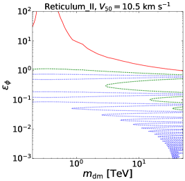
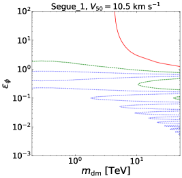
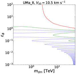
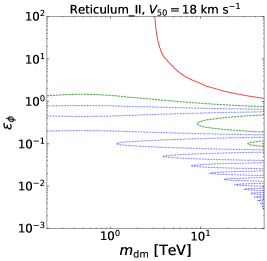
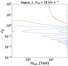
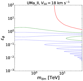
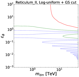
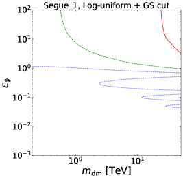
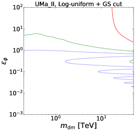
Figure 5: Expected upper limit contour of the annihilation cross section, $\sigma v\,[{\rm cm}^{3}\,{\rm s}^{-1}]=10^{-24}$ (solid red), $10^{-25}$ (dashed green), $10^{-26}$ (dotted blue) by CTA North with 500 hour experiment. We use median J-factor and the annihilation mode is assume to be $b\bar{b}$. Limits are given by observing Reticulum II, Segue 1, and Ursa Major II (left to right) and satellite prior with $V_{50}=$ 10.5 km s^-1 (top) and 18 km s^-1 (middle) are adopted. As a comparison, result using log-uniform prior with GS15 cut is given (bottom).

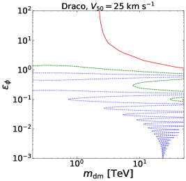
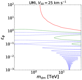
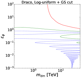
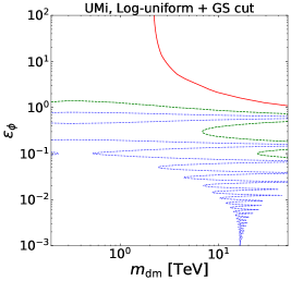
Figure 6: The same as Fig. 5 but analyzed for classical dSph, Draco and Ursa Minor. The parameters are the same as Fig. 2.

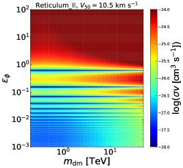
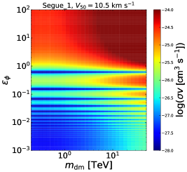
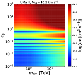
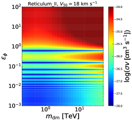
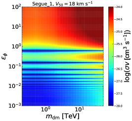
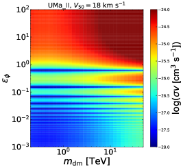
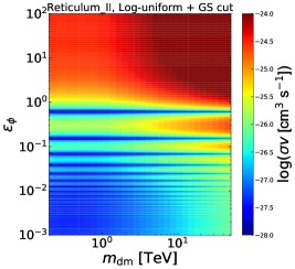
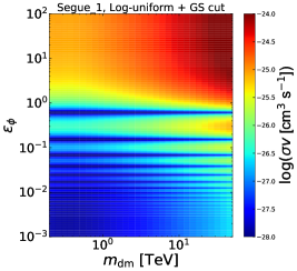
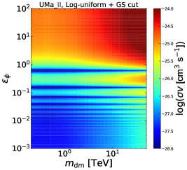
Figure 7: Colored map of the upper limit of the annihilation cross section. Parameters are the same as Fig. 5.

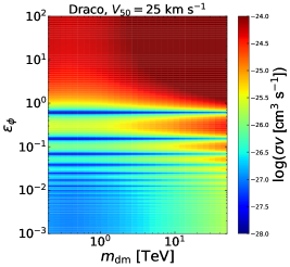
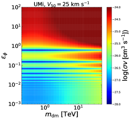
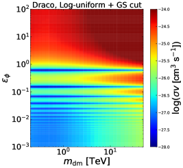
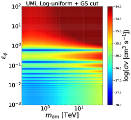
Figure 8: The same as Fig. 7 but for Draco and Ursa Minor and the parameters are the same as Fig. 6.

We are now ready to show the expected sensitivity of CTA North to the DM annihilation that is enhanced by the Sommerfeld effect. In Fig. 5, the expected upper limits using ultrafaint dSphs on the annihilation cross section in the light mediator model is shown. We assume that DM annihilates into $b\bar{b}$. In the plot, we use median J-factor computed in Sec. 3.1. As in Fig. 1, Reticulum II, Segue 1, and Ursa Major II are used in the analysis where the satellite prior with $V_{50}=$ 10.5 km s^-1 and 18 km s^-1 compared to log-uniform + GS15 cut prior. For all ultrafaint dSphs plotted here it is found that the results with satellite prior (with $V_{50}=10.5$ km s^-1) gives weaker upper limits compared to the log-uniform + GS15 cut prior. The most stringent bound is obtained from Segue 1. The result with $V_{50}=10.5$ km s^-1 shows that DM annihilation with $\sigma v=10^{-26}$ cm³ s^-1 can be detected in the mass range $m_{\rm dm}<\order{10\,{\rm TeV}}$ ($\order{1\,{\rm TeV}}$) for $\epsilon_{\phi}<\order{10^{-2}}$ ($\order{10^{-1}}$). The result with $V_{50}=18$ km s^-1, on the other hand, gives a bit more optimistic expectation; DM annihilation with $\sigma v=10^{-26}$ cm³ s^-1 can be detected in the mass range $m_{\rm dm}<\order{10\,{\rm TeV}}$ ($\order{1\,{\rm TeV}}$) for $\epsilon_{\phi}<\order{10^{-2}}$ ($\order{1}$). Fig. 6 shows the upper limits from classical dSphs: Draco and Ursa Minor. It is found that the constraints are comparable or weaker than Segue 1. For full information about the upper limits of the annihilation cross section, we provide the colored map in Figs. 7 and 8.

A comment on J-factor estimates of Segue 1 is in order. In order to estimate its density profile parameters, we adopt a velocity dispersion of the member stars based on Ref. [57]. However, there is a large uncertainty on what stars are regarded as a member of the system, and depending on their inclusion or exclusion, the estimates of the J factor of Segue 1 can be smaller by orders of magnitude [58, 59]. We caution that our estimates are on an optimistic side, in a similar spirit of earlier paper by the Magic collaboration [60]. Unlike earlier work including Ref. [60], however, our new modeling adopting satellite priors systematically shifts the best estimates of the J factors toward lower values, whereas our results in the case of uninformative priors are consistent with the results of the earlier studies.

We now move on to the sensitivity to the Wino DM. Fig. 9 shows the expected 95% CL upper limits on the $\sigma v_{\rm line}$ (defined in Eq. (48)) by observing ultrafaint dSphs, Reticulum II, Segue 1, and Ursa Major II. It has been found that all selected ultrafaint dSphs have the sensitivity to detect 2.7–3 TeV Wino DM. It is worth noticing that this conclusion is independent of the prior model. Namely in either model with $V_{50}=10.5$ km s^-1 or $18$ km s^-1, the result shows that the CTA observing those ultrafaint dSphs can detect the Wino DM with a mass of 2.7–3 TeV. The same conclusion is derived by observing classical dSphs, Draco and Ursa Minor (see Fig. 10). They can be promising for detection of the Wino DM. Therefore, it is concluded that the observation of dSphs by CTA will provide another robust avenue to look for the Wino DM in addition the Galactic center region [35].

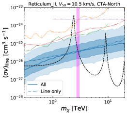
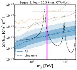
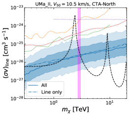
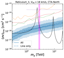
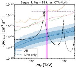
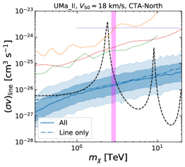
Figure 9: Expected 95% upper limits on $\sigma v_{\rm line}$ by CTA North with 500 hours of exposure for the Wino DM, for the ultrafaint dSphs:Reticulum II (left), Segue 1 (middle), and Ursa Major II (right). Top and bottom panels show the results corresponding to different satellite priors with $V_{50}=10.5$ and 18 km s^-1, respectively. The solid curve shows the expected median sensitivity at 95% CL, while thick and thin bands are 68% and 95% containment regions, respectively. Dotted curves are existing upper limits by the current generation of telescopes: HESS [61] (orange), MAGIC [60] (red), VERITAS [62] (green), and HAWC [63] (purple). The dashed curve shows the expected Wino annihilation cross section with the Sommerfeld enhancement, whereas purple vertical region highlights the most likely region of the Wino mass, 2.7–3 TeV.

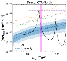
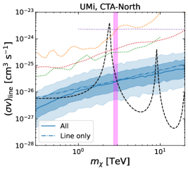
Figure 10: Same as Fig. 9, but for classical dSphs:Draco (left) and Ursa Minor (right). Satellite prior with $V_{50}=$25 km s^-1 is used.

5 Conclusions

In this paper we have studied the detection of DM whose annihilation process is enhanced by the Sommerfeld effect. To this end, we focus on observations of dSphs. In order to derive the current limits and the future sensitivities on the annihilation cross section of DM, it is crucial to determine the J-factor of the each dSph. Recently the J-factors of the dSphs were calculated by using proper theoretical priors and it was found that the J-factors were reduced by at least a factor of a few for ultrafaint dSphs [28]. By applying these satellite priors, we have calculated the J-factors of the dSphs for DM annihilating into the standard model particles enhanced by the Sommerfeld effect. We emphasize that most of the previous work on the dSph density profile estimates adopted uninformative log-flat priors for the density profile parameters such as $r_{s}$ and $\rho_{s}$. In this paper, therefore, we focused on evaluating the impact of adopting the new satellite priors in comparison with traditional uninformative priors. To be concrete, we have studied two models: (1) DM annihilation boosted by a light scalar mediator via the Yukawa interaction; and (2) Wino DM in supersymmetric models.

In the former case, the enhancement factor depends on the velocity of DM that is determined by the profile. Since the priors give probability distribution of the profile parameters, the prior dependence of the J-factor is non-trivial. By computing the J-factor with the priors, we have found that although J-factor rapidly oscillates as function of $\epsilon_{\phi}$, ratio of light mediator mass to DM mass times the Yukawa coupling squared, the relative difference of J-factors with different priors is less sensitive to $\epsilon_{\phi}$. In addition, assuming that DM self-annihilates into $b\bar{b}$ final state, we have calculated expected sensitivity limits on the annihilation cross section by the CTA on $\epsilon_{\phi}$ and DM mass plane by using different priors for ultrafaint and classical dSphs.

In the latter case, a free parameter in the DM sector of the Lagrangian is the Wino mass and the cross section is determined uniquely for a given Wino mass. Besides, the Wino mass is determined to be 2.7–3 TeV if the thermal freeze-out scenario is assumed. We have computed the Wino annihilation cross section at the next-to-leading log level following Ref. [53] and derived the current limits on the annihilation cross section and the future sensitivity by CTA observation. It has been found that measurements of one of the ultrafaint dSphs (Reticulum, Segue 1, and Ursa Major II) and classical dSphs (Draco and Ursa Minor) will give us sufficient sensitivity to detect the Wino DM with 2.7–3 TeV mass with CTA observations for 500 hours. This conclusion is nearly independent of the priors, thus it is a robust prediction. One should, however, keep in mind relatively large uncertainties related to the density profile estimates of Segue 1 ultrafaint dSph, when making a decision on which of these dSphs should be chosen as the best target. We conclude that observing dSphs is another powerful tool to detect the Wino DM as well as the observation of the Galactic center region.

References

- [1] Y. Akrami et al. [Planck], [arXiv:1807.06205 [astro-ph.CO]].
- [2] G. Giudice and A. Romanino, Nucl. Phys. B 699, 65-89 (2004) doi:10.1016/j.nuclphysb.2004.08.001 [arXiv:hep-ph/0406088 [hep-ph]].
- [3] G. F. Giudice and A. Strumia, Nucl. Phys. B 858, 63-83 (2012) doi:10.1016/j.nuclphysb.2012.01.001 [arXiv:1108.6077 [hep-ph]].
- [4] A. Arvanitaki, N. Craig, S. Dimopoulos and G. Villadoro, JHEP 02, 126 (2013) doi:10.1007/JHEP02(2013)126 [arXiv:1210.0555 [hep-ph]].
- [5] N. Arkani-Hamed, A. Gupta, D. E. Kaplan, N. Weiner and T. Zorawski, [arXiv:1212.6971 [hep-ph]].
- [6] L. J. Hall and Y. Nomura, JHEP 03, 076 (2010) doi:10.1007/JHEP03(2010)076 [arXiv:0910.2235 [hep-ph]].
- [7] L. J. Hall and Y. Nomura, JHEP 01, 082 (2012) doi:10.1007/JHEP01(2012)082 [arXiv:1111.4519 [hep-ph]].
- [8] M. Ibe and T. T. Yanagida, Phys. Lett. B 709, 374-380 (2012) doi:10.1016/j.physletb.2012.02.034 [arXiv:1112.2462 [hep-ph]].
- [9] M. Ibe, S. Matsumoto and T. T. Yanagida, Phys. Rev. D 85, 095011 (2012) doi:10.1103/PhysRevD.85.095011 [arXiv:1202.2253 [hep-ph]].
- [10] J. Hisano, K. Ishiwata and N. Nagata, JHEP 06, 097 (2015) doi:10.1007/JHEP06(2015)097 [arXiv:1504.00915 [hep-ph]].
- [11] J. Hisano, S. Matsumoto, M. M. Nojiri and O. Saito, Phys. Rev. D 71, 015007 (2005) doi:10.1103/PhysRevD.71.015007 [arXiv:hep-ph/0407168 [hep-ph]].
- [12] J. Hisano, K. Ishiwata and N. Nagata, Phys. Lett. B 690, 311-315 (2010) doi:10.1016/j.physletb.2010.05.047 [arXiv:1004.4090 [hep-ph]].
- [13] J. Hisano, K. Ishiwata and N. Nagata, Phys. Rev. D 82, 115007 (2010) doi:10.1103/PhysRevD.82.115007 [arXiv:1007.2601 [hep-ph]].
- [14] J. Hisano, K. Ishiwata, N. Nagata and T. Takesako, JHEP 07, 005 (2011) doi:10.1007/JHEP07(2011)005 [arXiv:1104.0228 [hep-ph]].
- [15] J. Hisano, K. Ishiwata and N. Nagata, Phys. Rev. D 87, 035020 (2013) doi:10.1103/PhysRevD.87.035020 [arXiv:1210.5985 [hep-ph]].
- [16] R. J. Hill and M. P. Solon, Phys. Lett. B 707, 539-545 (2012) doi:10.1016/j.physletb.2012.01.013 [arXiv:1111.0016 [hep-ph]].
- [17] R. J. Hill and M. P. Solon, Phys. Rev. Lett. 112, 211602 (2014) doi:10.1103/PhysRevLett.112.211602 [arXiv:1309.4092 [hep-ph]].
- [18] R. J. Hill and M. P. Solon, Phys. Rev. D 91, 043504 (2015) doi:10.1103/PhysRevD.91.043504 [arXiv:1401.3339 [hep-ph]].
- [19] R. J. Hill and M. P. Solon, Phys. Rev. D 91, 043505 (2015) doi:10.1103/PhysRevD.91.043505 [arXiv:1409.8290 [hep-ph]].
- [20] J. Hisano, S. Matsumoto and M. M. Nojiri, Phys. Rev. Lett. 92, 031303 (2004) doi:10.1103/PhysRevLett.92.031303 [arXiv:hep-ph/0307216 [hep-ph]].
- [21] J. Hisano, S. Matsumoto, M. M. Nojiri and O. Saito, Phys. Rev. D 71, 063528 (2005) doi:10.1103/PhysRevD.71.063528 [arXiv:hep-ph/0412403 [hep-ph]].
- [22] J. Hisano, S. Matsumoto, M. Nagai, O. Saito and M. Senami, Phys. Lett. B 646, 34-38 (2007) doi:10.1016/j.physletb.2007.01.012 [arXiv:hep-ph/0610249 [hep-ph]].
- [23] M. Beneke, A. Bharucha, F. Dighera, C. Hellmann, A. Hryczuk, S. Recksiegel and P. Ruiz-Femenia, JHEP 03, 119 (2016) doi:10.1007/JHEP03(2016)119 [arXiv:1601.04718 [hep-ph]].
- [24] N. Arkani-Hamed, D. P. Finkbeiner, T. R. Slatyer and N. Weiner, Phys. Rev. D 79, 015014 (2009) doi:10.1103/PhysRevD.79.015014 [arXiv:0810.0713 [hep-ph]].
- [25] J. D. Simon, Ann. Rev. Astron. Astrophys. 57, no.1, 375-415 (2019) doi:10.1146/annurev-astro-091918-104453 [arXiv:1901.05465 [astro-ph.GA]].
- [26] V. Springel, J. Wang, M. Vogelsberger, A. Ludlow, A. Jenkins, A. Helmi, J. F. Navarro, C. S. Frenk and S. D. M. White, Mon. Not. Roy. Astron. Soc. 391, 1685-1711 (2008) doi:10.1111/j.1365-2966.2008.14066.x [arXiv:0809.0898 [astro-ph]].
- [27] A. Geringer-Sameth, S. M. Koushiappas and M. Walker, Astrophys. J. 801, no.2, 74 (2015) doi:10.1088/0004-637X/801/2/74 [arXiv:1408.0002 [astro-ph.CO]].
- [28] S. Ando, A. Geringer-Sameth, N. Hiroshima, S. Hoof, R. Trotta and M. G. Walker, [arXiv:2002.11956 [astro-ph.CO]].
- [29] S. Hoof, A. Geringer-Sameth and R. Trotta, JCAP 02, 012 (2020) doi:10.1088/1475-7516/2020/02/012 [arXiv:1812.06986 [astro-ph.CO]].
- [30] K. K. Boddy, J. Kumar, L. E. Strigari and M. Y. Wang, Phys. Rev. D 95, no.12, 123008 (2017) doi:10.1103/PhysRevD.95.123008 [arXiv:1702.00408 [astro-ph.CO]].
- [31] B. Q. Lu, Y. L. Wu, W. H. Zhang and Y. F. Zhou, JCAP 04, 035 (2018) doi:10.1088/1475-7516/2018/04/035 [arXiv:1711.00749 [astro-ph.HE]].
- [32] M. Petac, P. Ullio and M. Valli, JCAP 12, 039 (2018) doi:10.1088/1475-7516/2018/12/039 [arXiv:1804.05052 [astro-ph.GA]].
- [33] S. Bergström, R. Catena, A. Chiappo, J. Conrad, B. Eurenius, M. Eriksson, M. Högberg, S. Larsson, E. Olsson, A. Unger and R. Wadman, Phys. Rev. D 98, no.4, 043017 (2018) doi:10.1103/PhysRevD.98.043017 [arXiv:1712.03188 [astro-ph.CO]].
- [34] L. Rinchiuso, O. Macias, E. Moulin, N. L. Rodd and T. R. Slatyer, Phys. Rev. D 103, no.2, 023011 (2021) doi:10.1103/PhysRevD.103.023011 [arXiv:2008.00692 [astro-ph.HE]].
- [35] L. Rinchiuso, N. L. Rodd, I. Moult, E. Moulin, M. Baumgart, T. Cohen, T. R. Slatyer, I. W. Stewart and V. Vaidya, Phys. Rev. D 98, no.12, 123014 (2018) doi:10.1103/PhysRevD.98.123014 [arXiv:1808.04388 [astro-ph.HE]].
- [36] A. Hryczuk, K. Jodlowski, E. Moulin, L. Rinchiuso, L. Roszkowski, E. M. Sessolo and S. Trojanowski, JHEP 10, 043 (2019) doi:10.1007/JHEP10(2019)043 [arXiv:1905.00315 [hep-ph]].
- [37] V. Lefranc, E. Moulin, P. Panci, F. Sala and J. Silk, JCAP 09, 043 (2016) doi:10.1088/1475-7516/2016/09/043 [arXiv:1608.00786 [astro-ph.HE]].
- [38] https://www.cta-observatory.org
- [39] B. S. Acharya et al. [CTA Consortium], doi:10.1142/10986 [arXiv:1709.07997 [astro-ph.IM]].
- [40] N. Hiroshima, S. Ando and T. Ishiyama, Phys. Rev. D 97, no.12, 123002 (2018) doi:10.1103/PhysRevD.97.123002 [arXiv:1803.07691 [astro-ph.CO]].
- [41] A. S. Graus, J. S. Bullock, T. Kelley, M. Boylan-Kolchin, S. Garrison-Kimmel, and Y. Qi, Mon. Not. Roy. Astron. Soc. 488 no. 4, (Oct, 2019) 4585–4595.
- [42] T. Ishiyama, J. Makino, S. Portegies Zwart, D. Groen, K. Nitadori, S. Rieder, C. de Laat, S. McMillan, K. Hiraki and S. Harfst, Astrophys. J. 767, 146 (2013) doi:10.1088/0004-637X/767/2/146 [arXiv:1101.2020 [astro-ph.CO]].
- [43] C. A. Correa, J. S. B. Wyithe, J. Schaye and A. R. Duffy, Mon. Not. Roy. Astron. Soc. 452, no.2, 1217-1232 (2015) doi:10.1093/mnras/stv1363 [arXiv:1502.00391 [astro-ph.CO]].
- [44] J. Penarrubia, A. J. Benson, M. G. Walker, G. Gilmore, A. McConnachie and L. Mayer, Mon. Not. Roy. Astron. Soc. 406, 1290 (2010) doi:10.1111/j.1365-2966.2010.16762.x [arXiv:1002.3376 [astro-ph.GA]].
- [45] F. Jiang and F. C. van den Bosch, Mon. Not. Roy. Astron. Soc. 458, no.3, 2848-2869 (2016) doi:10.1093/mnras/stw439 [arXiv:1403.6827 [astro-ph.CO]].
- [46] C. A. Correa, J. S. B. Wyithe, J. Schaye and A. R. Duffy, Mon. Not. Roy. Astron. Soc. 450, no.2, 1514-1520 (2015) doi:10.1093/mnras/stv689 [arXiv:1409.5228 [astro-ph.GA]].
- [47] J. R. Bond, S. Cole, G. Efstathiou and N. Kaiser, Astrophys. J. 379, 440 (1991) doi:10.1086/170520
- [48] X. Yang, H. J. Mo, Y. Zhang and F. C. v. d. Bosch, Astrophys. J. 741, 13 (2011) doi:10.1088/0004-637X/741/1/13 [arXiv:1104.1757 [astro-ph.CO]].
- [49] J. Binney and S. Tremaine,“ Galactic Dynamics: Second Edition”, Princeton University Press, Princeton U.S.A. (2008).
- [50] E. Vasiliev and V. Belokurov, Mon. Not. Roy. Astron. Soc. 497, 4162 (2020) 10.1093/mnras/staa2114 [arXiv:2006.02929 [astro-ph.GA]].
- [51] M. Ibe, S. Matsumoto and R. Sato, Phys. Lett. B 721, 252-260 (2013) doi:10.1016/j.physletb.2013.03.015 [arXiv:1212.5989 [hep-ph]].
- [52] M. Baumgart, T. Cohen, I. Moult, N. L. Rodd, T. R. Slatyer, M. P. Solon, I. W. Stewart and V. Vaidya, JHEP 03, 117 (2018) doi:10.1007/JHEP03(2018)117 [arXiv:1712.07656 [hep-ph]].
- [53] M. Baumgart, T. Cohen, E. Moulin, I. Moult, L. Rinchiuso, N. L. Rodd, T. R. Slatyer, I. W. Stewart and V. Vaidya, JHEP 01, 036 (2019) doi:10.1007/JHEP01(2019)036 [arXiv:1808.08956 [hep-ph]].
- [54] M. Beneke, A. Broggio, C. Hasner, K. Urban and M. Vollmann, JHEP 08, 103 (2019) [erratum: JHEP 07, 145 (2020)] doi:10.1007/JHEP08(2019)103 [arXiv:1903.08702 [hep-ph]].
- [55] M. Beneke, R. Szafron and K. Urban, JHEP 02, 020 (2021) doi:10.1007/JHEP02(2021)020 [arXiv:2009.00640 [hep-ph]].
- [56] H. Silverwood, C. Weniger, P. Scott and G. Bertone, JCAP 03, 055 (2015) doi:10.1088/1475-7516/2015/03/055 [arXiv:1408.4131 [astro-ph.HE]].
- [57] J. D. Simon, M. Geha, Q. E. Minor, G. D. Martinez, E. N. Kirby, J. S. Bullock, M. Kaplinghat, L. E. Strigari, B. Willman and P. I. Choi, et al. Astrophys. J. 733 (2011), 46 doi:10.1088/0004-637X/733/1/46 [arXiv:1007.4198 [astro-ph.GA]].
- [58] V. Bonnivard, C. Combet, M. Daniel, S. Funk, A. Geringer-Sameth, J. A. Hinton, D. Maurin, J. I. Read, S. Sarkar and M. G. Walker, et al. Mon. Not. Roy. Astron. Soc. 453 (2015) no.1, 849-867 doi:10.1093/mnras/stv1601 [arXiv:1504.02048 [astro-ph.HE]].
- [59] K. Hayashi, K. Ichikawa, S. Matsumoto, M. Ibe, M. N. Ishigaki and H. Sugai, Mon. Not. Roy. Astron. Soc. 461 (2016) no.3, 2914-2928 doi:10.1093/mnras/stw1457 [arXiv:1603.08046 [astro-ph.GA]].
- [60] J. Aleksić, S. Ansoldi, L. A. Antonelli, P. Antoranz, A. Babic, P. Bangale, U. Barres de Almeida, J. A. Barrio, J. Becerra González and W. Bednarek, et al. JCAP 02 (2014), 008 doi:10.1088/1475-7516/2014/02/008 [arXiv:1312.1535 [hep-ph]].
- [61] H. Abdalla et al. [HESS], JCAP 11 (2018), 037 doi:10.1088/1475-7516/2018/11/037 [arXiv:1810.00995 [astro-ph.HE]].
- [62] S. Archambault et al. [VERITAS], Phys. Rev. D 95 (2017) no.8, 082001 doi:10.1103/PhysRevD.95.082001 [arXiv:1703.04937 [astro-ph.HE]].
- [63] A. Albert et al. [HAWC], Phys. Rev. D 101 (2020) no.10, 103001 doi:10.1103/PhysRevD.101.103001 [arXiv:1912.05632 [astro-ph.HE]].