Self-supervised Symmetric Nonnegative Matrix Factorization

Abstract

Symmetric nonnegative matrix factorization (SNMF) has demonstrated to be a powerful method for data clustering. However, SNMF is mathematically formulated as a non-convex optimization problem, making it sensitive to the initialization of variables. Inspired by ensemble clustering that aims to seek a better clustering result from a set of clustering results, we propose self-supervised SNMF (S³NMF), which is capable of boosting clustering performance progressively by taking advantage of the sensitivity to initialization characteristic of SNMF, without relying on any additional information. Specifically, we first perform SNMF repeatedly with a random nonnegative matrix for initialization each time, leading to multiple decomposed matrices. Then, we rank the quality of the resulting matrices with adaptively learned weights, from which a new similarity matrix that is expected to be more discriminative is reconstructed for SNMF again. These two steps are iterated until the stopping criterion/maximum number of iterations is achieved. We mathematically formulate S³NMF as a constraint optimization problem, and provide an alternative optimization algorithm to solve it with the theoretical convergence guaranteed. Extensive experimental results on $10$ commonly used benchmark datasets demonstrate the significant advantage of our S³NMF over $12$ state-of-the-art methods in terms of $5$ quantitative metrics. The source code is publicly available at https://github.com/jyh-learning/SSSNMF.

I Introduction

Nonnegative matrix factorization (NMF) [1, 2, 3] is a well-known dimensionality reduction method for data representation. Technically, it decomposes a nonnegative matrix as the product of two smaller nonnegative matrices named the basis matrix and the embedding matrix. Due to the nonnegative constraints on both the input matrix and the factorized matrices, NMF is able to learn a parts-based representation. Taking face images as an example, the basis matrix contains the meaningful parts of the input face, e.g., a nose or an eye, and the embedding matrix assembles the bases to recover the face. Such a unique feature enables the success of NMF in many applications, e.g., topic modeling [4], hyperspectral image unmixing [5], blind audio source separation [6], image classification [7], visual tracking [8, 9], etc. See the comprehensive review of NMF in [10] and [11].

In addition to data representation, NMF has been used to solve various clustering problems [12], e.g., tumor clustering [13], community detection [14], document clustering [15], and so on. Particularly, Ding et al. [16] revealed the equivalence between NMF and K-means. However, NMF is only effective for partitioning linearly separable data and usually cannot exploit the non-linear relationship of the input [17]. To solve this drawback, symmetric NMF (SNMF) was proposed [18, 19]. Different from NMF that factorizes the sample matrix into two different matrices, SNMF decomposes an affinity matrix that records the pairwise similarity of samples as the product of a nonnegative matrix and its transpose. Kuang et al. [19] showed that SNMF is related to spectral clustering (SC) [20], and both of them share the same loss function only with different constraints. Therefore, SNMF can be regarded as a graph clustering method [19], and it is more effective for nonlinearly separable data than NMF. Another merit of SNMF is that it can directly generate the clustering indicator without post-processing, while SC needs extra post-processing like K-means to finalize clustering.

A number of advanced SNMF methods were proposed to enhance the clustering ability of SNMF. For example, to encode the geometry structure of data samples, Gao et al. [21] proposed to use a local graph to regularize the decomposition of SNMF. Considering the input affinity matrix affects the performance of SNMF severely, Jia et al. [22] proposed to learn an adaptive affinity matrix from data samples rather than use an empirically defined one, and perform SNMF simultaneously. Zhang et al. [23] extended SNMF to solve the multi-view clustering problem. Besides, many semi-supervised SNMF models were proposed to encode the available supervisory information. For example, Yang et al. [24] proposed to use the supervisory information to regularize SNMF. Wu et al. [25] took advantage of the supervisory information by using them to construct a superior affinity matrix. Although different kinds of optimization methods were proposed, e.g., Newton method [19], alternating nonnegative least squares [26], and multiplicative update [27], and block coordinate descent [28], etc., SNMF is essentially a non-convex optimization problem, and its sensitivity to initialization is inevitable, i.e., the clustering performance of SNMF heavily relies on the initialization, and a bad initialization matrix will degrade clustering performance significantly.

Motivated by ensemble clustering [29, 22], i.e., multiple clustering results obtained by different kinds of clustering methods could generate a better one, we propose self-supervised SNMF (S³NMF), which is able to boost clustering performance progressively by taking advantage of the sensitivity to initialization characteristic of SNMF without relying on any additional information. Specifically, we perform SNMF repeatedly with a random nonnegative matrix for initialization each time, leading to multiple decomposed matrices. Then, we rank the quality of those matrices adaptively, and form a new affinity matrix from their binarizations (named clustering partition) under the guidance of their ranking. As the clustering partition of an affinity matrix is usually more discriminative than the relationships between samples encoded in the affinity matrix (because an imperfect affinity matrix could produce a perfect partition [22, 29]), it is expected that the newly constructed affinity matrix is superior to the original one. Then, we further learn a set of new clustering partitions from the newly constructed affinity matrix via SNMF. Such two steps are repeated until the proposed stopping criterion is satisfied. During the iteration, the clustering performance grows progressively. Mathematically, we explicitly cast S³NMF as a constrained optimization problem, and provide an efficient and effective algorithm to solve it with the theoretical convergence guaranteed. Moreover, we give empirical values for the hyper-parameters, making it easy to use. We compare the proposed model with 12 state-of-the-art methods on 10 datasets in terms of 5 clustering metrics. The extensive experimental comparisons substantiate the superior performance of the proposed model, and also validates the effectiveness of the stopping criterion as well as the empirical values.

The rest of this paper is organized as follows. We first introduce the background of NMF and SNMF in Section II. In Section III, we present the proposed model and its numerical solution as well as the theoretical analyses. In Section IV, we experimentally validate the advantages of the proposed method. Finally, we conclude this paper in Section V.

II Related Work

In this section, we first introduce NMF and the basic SNMF, followed by advanced SNMF-based mehtods.

II-A Nonnegative Matrix Factorization

Let $\mathbf{X}=[\mathbf{x}_{1},\cdots,\mathbf{x}_{n}]\in\mathbb{R}^{d\times n}$ denote the input nonnegative matrix with $n$ samples, where $\mathbf{x}_{i}\in\mathbb{R}^{d}$ is the vectorial representation of the $i$-th sample of dimension $d$. As a powerful and popular dimensionality reduction method, NMF factorizes $\mathbf{X}$ as the product of two smaller nonnegative matrices [30], i.e.,

$$\begin{split}\min_{\mathbf{U},\mathbf{V}}\left\|\mathbf{X}-\mathbf{U}\mathbf{V}^{\mathsf{T}}\right\|_{F}^{2},{\rm s.t.~{}}\mathbf{U}\geq 0,\mathbf{V}\geq 0,\end{split}$$ (1)

where $\mathbf{U}=[\mathbf{u}_{1},\cdots,\mathbf{u}_{k}]\in\mathbb{R}^{d\times k}$ is the basis matrix, $\mathbf{V}=[\mathbf{v}_{1},\cdots,\mathbf{v}_{n}]^{\mathsf{T}}\in\mathbb{R}^{n\times k}$ is the low-dimensional representation, $k$ is the dimension of the new representation, $\mathbf{U}\geq 0,\mathbf{V}\geq 0$ mean that each element of $\mathbf{U}$ and $\mathbf{V}$ is nonnegative, and $\|\cdot\|_{F}$ and $\cdot^{\mathsf{T}}$ indicate the Frobenius norm and the transpose of a matrix, respectively. The conventional NMF requires the input matrix $\mathbf{X}$ to be nonnegative. This assumption is reasonable for many real-world signals as they can be naturally represented with nonnegative values, such as pixels of an image, the acoustic signals, and the spectral signature of hyperspectral images. Together with the fact that the outputs $\mathbf{U}$ and $\mathbf{V}$ are also nonnegative, NMF only allows additive operations, i.e., each sample $\mathbf{x}_{i}$ is reconstructed by the conical combination of columns of $\mathbf{U}$, where $\mathbf{v}_{i}$ is the combination coefficient vector. This means that each column of $\mathbf{U}$ should only be part of $\mathbf{X}$, leading to an interpretable parts-based representation. Owing to the parts-based representation, NMF has been applied in many real-world applications. Especially, NMF has acted as a clustering method [12]. Ding et al. [16] pointed out that NMF is a soft version of K-means clustering. Together with the good data representation ability, the clustering performance of NMF is excellent in many problems, like tumor clustering [13], community detection [14], face clustering [31] and document clustering [15].

II-B Symmetric Nonnegative Matrix Factorization

The conventional NMF is effective for linear-spreadable data and usually fails to cope with non-linear data [17]. To this end, as a variant of NMF, SNMF [19] was proposed to play as a graph clustering method, which is effective for handling non-linear data [17]. Different from NMF, SNMF decomposes an affinity matrix as the product of a nonnegative matrix and its transpose, i.e.,

$$\begin{split}\min_{\mathbf{V}}\left\|\mathbf{W}-\mathbf{V}\mathbf{V}^{\mathsf{T}}\right\|_{F}^{2},{\rm s.t.~{}}\mathbf{V}\geq 0,\end{split}$$ (2)

where $\mathbf{W}\in\mathbb{R}^{n\times n}$ is the affinity matrix recording the pairwise relationship between samples, and $\mathbf{V}\in\mathbb{R}^{n\times k}$ is the factorized matrix. SNMF is highly related to the well-known spectral clustering (SC) [20]. Concretely, the objective of SC can be formulated as

$$\begin{split}\min_{\mathbf{V}}\left\|\mathbf{W}-\mathbf{V}\mathbf{V}^{\mathsf{T}}\right\|_{F}^{2},{\rm s.t.~{}}\mathbf{V}^{\mathsf{T}}\mathbf{V}=\mathbf{I},\end{split}$$ (3)

where $\mathbf{I}\in\mathbb{R}^{k\times k}$ is the identity matrix. Comparing Eq. (2) with Eq.(3), we can see that SC and SNMF share the same objective function but with different constraints. Particularity, SC seeks an orthogonal decomposition, while SNMF learns a nonnegative embedding. The same objective function reveals why SNMF is capable of acting as a general graph clustering method, while the different constraints increase the interpretability of the factorized matrix of SNMF, i.e., the location of the largest value of $\mathbf{v}_{i}$ can indicate the cluster membership of sample $\mathbf{x}_{i}$ [19]. Specifically, for SNMF, the partition matrix (or clustering membership matrix) $\mathbf{M}\in\mathbb{R}^{n\times k}$ is obtained by

$$\mathbf{M}_{ij}=\begin{cases}1,~{}{\rm if}~{}\mathbf{V}_{ij}=\max_{j}\mathbf{V}_{ij}\\ 0,~{}{\rm others},\end{cases}$$ (4)

where $\mathbf{M}_{ij}$ and $\mathbf{V}_{ij}$ are the $(i,j)$-th entries of $\mathbf{M}$ and $\mathbf{V}$, respectively. In SNMF, we could set $k=c$ with $c$ being the number of clusters. This is one of the main advantages of SNMF over SC that needs to perform the K-means algorithm on $\mathbf{V}$ to obtain the final clustering result.

Plenty of SNMF-based clustering methods were proposed. For example, Gao et al. [21] proposed graph regularized SNMF for clustering, which is formulated as

$$\begin{split}\min_{\mathbf{V}}\left\|\mathbf{W}-\mathbf{V}\mathbf{V}^{\mathsf{T}}\right\|_{F}^{2}+\lambda{\rm tr}\left(\mathbf{V}^{\mathsf{T}}\mathbf{LV}\right),{\rm s.t.~{}}\mathbf{V}\geq 0,\end{split}$$ (5)

where the Laplacian graph $\mathbf{L}\in\mathbb{R}^{n\times n}$ is utilized to incorporate the local structure of the input into SNMF. Being aware of the importance of the input affinity matrix, Jia et al. [22] proposed to adaptively learn an affinity matrix from the samples rather than use a predefined one, i.e.,

$$\begin{split}&\min_{\mathbf{V},\mathbf{S}}\|\mathbf{X}-\mathbf{XS}\|_{F}^{2}+\lambda\left\|\mathbf{S}-\mathbf{V}\mathbf{V}^{\mathsf{T}}\right\|_{F}^{2}+\mu\|\mathbf{S}-\mathbf{W}\|_{F}^{2}\\ &{\rm s.t.~{}}\mathbf{V}\geq 0,\mathbf{S}\geq 0,{\rm diag}(\mathbf{S})=0,\end{split}$$ (6)

where $\mathbf{S}\in\mathbb{R}^{n\times n}$ is the learned affinity matrix, and $\mathbf{W}$ is the empirically built affinity matrix. Eq. (6) could simultaneously perform clustering and learn the affinity matrix to achieve a mutual enhancement. SNMF was also extended to solve the multi-view clustering problem [23, 32] and the multi-task clustering problem [33, 34]. Since SNMF is performed on an affinity matrix, SNMF-based methods have been developed as an essential tool in correlation modeling [35], network analysis [36], link prediction [37], and community detection [38, 24]. Moreover, many semi-supervised SNMF models were proposed to incorporate the available supervisory information [24, 27, 25, 17], which can generate better clustering performance than the unsupervised one.

Both the basic SNMF and the above-mentioned advanced models involve solving a 4-th order non-convex optimization problem of $\mathbf{V}$ with the nonnegative constraint iteratively, and there is no closed-form solutions for them. In general, taking the basic SNMF as an example, $\mathbf{V}$ is updated iteratively to optimize Eq. (2) from a random initialization matrix $\mathbf{V}^{0}\in\mathbb{R}^{n\times c}$, i.e., $\mathbf{V}^{0}\rightarrow\cdots\mathbf{V}^{t-1}\rightarrow\mathbf{V}^{t}\cdots$, where $t$ is the iteration index. In each iteration, the loss function is non-increased, i.e., $\|\mathbf{W}-\mathbf{V}^{t}\mathbf{V}^{{t}^{\mathsf{T}}}\|\leq\|\mathbf{W}-\mathbf{V}^{t-1}\mathbf{V}^{{t-1}^{\mathsf{T}}}\|$. However, the objective function of SNMF is non-convex, and thus, the initialization matrix $\mathbf{V}^{0}$ will severely affect the final solution $\mathbf{V}^{*}$. This means that some poor initialization matrices will lead to inferior clustering results, which limits the application of SNMF.

III Proposed model

As earlier mentioned, SNMF needs to solve a non-convex optimization problem, which is sensitive to the initialization of variables. By utilizing such a sensitivity characteristic of SNMF, we propose self-supervised SNMF (S³NMF), which is capable of progressively boosting clustering performance without relying on any additional information. To be specific, S³NMF is inspired by the success of ensemble clustering that aims to seek a consensus and better clustering result from a number of clustering results obtained by different kinds of clustering methods [39] via exploiting the coherence among them. Due to the sensitivity of SNMF to the initialization of variables, we can treat the decomposed matrices of SNMF with various random initialization as diverse clustering results. Thus, our S³NMF boils down to how to improve the clustering performance of SNMF with different initialization.

Unlike the SNMF in Eq. (2), where the variable is initialized with a single random nonnegative matrix $\mathbf{V}^{0}$, we first generate a set of random nonnegative matrices denoted as $\{\mathbf{V}^{0}_{m}\in\mathbb{R}^{n\times c}\}|_{m=1}^{b}$, where $b$ is the size of the set, and thus we can obtain $b$ clustering partitions denoted as $\{\mathbf{M}_{m}\}|_{m=1}^{b}$ after SNMF. Considering that each $\mathbf{M}_{m}$ is usually more discriminative than the original similarity matrix $\mathbf{W}$, we could form a superior affinity matrix $\mathbf{S}$ as

$$\mathbf{S}=\sum_{m=1}^{b}\alpha_{m}\mathbf{M}_{m}\mathbf{M}_{m}^{\mathsf{T}},$$ (7)

where $\alpha_{m}$ is the $m$-th element of $\bm{\alpha}\in\mathbb{R}^{b\times 1}$, the weight vector balancing the contribution of each partition whose derivation will be introduced later. With $\mathbf{S}$ obtained, we can generate a group of new and better clustering partitions under multiple initialization again. This process is repeated until the stopping criterion or maximum number of iterations is achieved.

Explicitly, we formulate the above procedure as a constrained optimization model, i.e.,

$$\begin{split}&\min_{\mathbf{V}_{m},\mathbf{S},\bm{\alpha}}\sum_{m=1}^{b}\mathbf{\alpha}_{m}\left\|\mathbf{S}-\mathbf{V}_{m}\mathbf{V}_{m}^{\mathsf{T}}\right\|_{F}^{2}\\ &{\rm s.t.~{}}\mathbf{V}_{m}\geq 0,\forall m,\bm{\alpha}\mathbf{1}=1,\bm{\alpha}\geq 0,\end{split}$$ (8)

where $\mathbf{1}\in\mathbb{R}^{b\times 1}$ denotes the all one vector, the constraint $\bm{\alpha}\mathbf{1}=1$ avoids the trivial solution of $\bm{\alpha}$ (i.e., $\bm{\alpha}=0$), and $\bm{\alpha}\geq 0$ guarantees that each ${\alpha}_{m}$ is a valid weight. Intuitively, by minimizing Eq. (8), a good (resp. poor) $\mathbf{V}_{m}$ will produce a smaller (resp. larger) $\|\mathbf{S}-\mathbf{V}_{m}\mathbf{V}_{m}^{\mathsf{T}}\|_{F}^{2}$ and likewise a larger (resp. smaller) $\mathbf{\alpha}_{m}$. Therefore, the value of $\mathbf{\alpha}_{m}$ could measure the quality of $\mathbf{V}_{m}$, and be further employed to construct $\mathbf{S}$ in Eq. (7). However, due to the nonnegative constraint on $\bm{\alpha}$, Eq. (8) imposes an implicit weighted $\ell_{1}$ norm on $\bm{\alpha}$. This may result in a quite sparse solution when optimizing Eq. (8), i.e., the majority of $\bm{\alpha}$ will be or quite close to $0$. As we aim to leverage the power of multiple clustering partitions, an extreme sparse $\bm{\alpha}$ is not a perfect choice. To this end, we introduce a hyper-parameter $\tau$ to control the distribution of the entries of $\bm{\alpha}$, and the final model is written as

$$\begin{split}&\min_{\mathbf{V}_{m},\mathbf{S},\bm{\alpha}}\sum_{m=1}^{b}(\mathbf{\alpha}_{m})^{\tau}\left\|\mathbf{S}-\mathbf{V}_{m}\mathbf{V}_{m}^{\mathsf{T}}\right\|_{F}^{2}\\ &{\rm s.t.~{}}\mathbf{V}_{m}\geq 0,\forall m,\bm{\alpha}\mathbf{1}=1,\bm{\alpha}\geq 0,\end{split}$$ (9)

where $\tau$ lies in the range of $(1,+\infty)$. When $\tau$ is close to $1$, only a few entries of $\bm{\alpha}$ will dominate the vector, while, when $\tau$ tends to $+\infty$, minimizing Eq. (9) will assign equal weights to $\bm{\alpha}$. Therefore, $\tau$ should be neither too large or too small. Thus, the value of $\tau$ is empirically set to $2$, and the influence of $\tau$ is experimentally investigated in Section IV.D. After solving Eq. (9), we can obtain a set of clustering partitions $\{\mathbf{M}_{m}\}|_{m=1}^{b}$, a better affinity matrix $\mathbf{S}$, and an estimated quality measure vector $\bm{\alpha}$.

Remark. It is worth pointing out that S³NMF is different from the existing ensemble clustering methods, which require a number of clustering partitions by different kinds of clustering methods as the input. The proposed model only needs an affinity matrix as the input, which is identical to the basic SNMF.

To solve Eq (9), we propose an alternating iterative method. First, with a fixed $\mathbf{S}$ as well as multiple random nonnegative initialization matrices $\mathbf{V}_{m}^{0}$s, we solve $\mathbf{V}_{m},\forall m$ and $\bm{\alpha}$ by

$$\begin{split}&\min_{\mathbf{V}_{m},\bm{\alpha}}\sum_{m=1}^{b}(\mathbf{\alpha}_{m})^{\tau}\left\|\mathbf{S}-\mathbf{V}_{m}\mathbf{V}_{m}^{\mathsf{T}}\right\|_{F}^{2}\\ &{\rm s.t.~{}}\mathbf{V}_{m}\geq 0,\forall m,\bm{\alpha}\mathbf{1}=1,\bm{\alpha}\geq 0.\end{split}$$ (10)

See the detailed solution of Eq. (10) in Section III.B. Then, fixing $\mathbf{V}_{m},\forall m$ and $\bm{\alpha}$ as those previously obtained, we update $\mathbf{S}$ via Eq. (7). Those two steps are performed alternatively and iteratively. See Algorithm 1 for the detailed description.

Algorithm 1 The Proposed S³NMF

0:  $\mathbf{W}$, $\tau=2$, $b$;

0:  iter=$1$, maxIter=$10$, $\mathbf{S}=\mathbf{W}$;

1:  while iter $<$ maxIter do

2:     Update $\mathbf{V}_{m},\forall m$ and $\bm{\alpha}$ via Algoithm 2;

3:     Update $\mathbf{S}$ by Eq. (7);

4:     if the stopping criterion is meet then

5:        break;

6:     end if

7:     iter= iter +1;

8:  end while

9:  Generate clustering membership matrces $\{\mathbf{M}_{m}\}|_{m=1}^{b}$ by Eq. (4);

Output: a group of clustering results $\{\mathbf{M}_{m}\}_{m=1}^{b}$.

III-A Stopping Criterion of Algorithm 1

We propose a simple yet effective criterion to terminate Algorithm 1 adaptively. It is reasonable to assume that at the first a few iterations, the clustering performance of all the partitions could be improved progressively, and the consensus across them can also be increased. When the largest consensus is achieved, the consensus across them will keep at such a high level or even might decrease and fluctuate due to the randomness in the initialization of variables at that iteration. Therefore, we leverage the level of consensus across different partitions to construct the stopping criterion.

Mutual information is a quantity that measures the relationship between two random variables. We treat the clustering results of two partitions as two sets of random variables, and then use the normalized mutual information (NMI) to assess their correlation, i.e.,

$${\rm NMI}_{ij}=\frac{\mathcal{I}\left(\mathbf{M}_{i},\mathbf{M}_{j}\right)}{\left(\mathcal{H}(\mathbf{M}_{i})+\mathcal{H}(\mathbf{M}_{j})\right)/2},$$ (11)

where $\mathcal{I}\left(\mathbf{M}_{i},\mathbf{M}_{j}\right)$ denotes the mutual information between partitions $i$ and $j$, and $\mathcal{H}(\mathbf{M}_{i})$ is the entropy of $\mathbf{M}_{i}$. The normalized version is adopted as the value of ${\rm NMI}_{ij}$ will be in the range of $[0,1]$ for all the sets of random variables. Based on NMI, we use the average NMI (ANMI) to measure the consensus level of all the partitions, i.e.,

$${\rm ANMI}=\frac{1}{b(b-1)}\sum_{i=1}^{b}\sum_{j=i+1}^{b}{\rm NMI}_{ij}.$$ (12)

ANMI lies in the range of $[0,1]$, and a larger ANMI indicates a higher level of consensus across different partitions. We terminate Algorithm 1 when the value of ANMI begins to drop, and take the outputs of the iteration with the highest ANMI as the final clustering result.

III-B Numerical Solution to Eq. (10)

Eq. (10) is non-convex, and thus quite challenging to solve. To tackle this challenge, we propose to optimize $\mathbf{V}_{m},\forall m$ and $\bm{\alpha}$ alternatively and iteratively, i.e., update $\mathbf{V}_{m},\forall m$ with a fixed $\bm{\alpha}$, and then update $\bm{\alpha}$ with a fixed $\mathbf{V}_{m},\forall m$.

III-B1 Update $\mathbf{V}$

With a fixed $\bm{\alpha}$, the $\mathbf{V}$-subproblem is expressed as

$$\begin{split}&\min_{\mathbf{V}_{m}}\sum_{m=1}^{b}(\mathbf{\alpha}_{m})^{\tau}\left\|\mathbf{S}-\mathbf{V}_{m}\mathbf{V}_{m}^{\mathsf{T}}\right\|_{F}^{2},~{}{\rm s.t.~{}}\mathbf{V}_{m}\geq 0,\forall m.\end{split}$$ (13)

As the $b$ decomposed matrices are independent of each other, we could solve each $\mathbf{V}_{m}$ separately. Specifically, for a typical one, the subproblem is written as

$$\begin{split}&\min_{\mathbf{V}_{m}}(\mathbf{\alpha}_{m})^{\tau}\left\|\mathbf{S}-\mathbf{V}_{m}\mathbf{V}_{m}^{\mathsf{T}}\right\|_{F}^{2},~{}{\rm s.t.~{}}\mathbf{V}_{m}\geq 0.\end{split}$$ (14)

Eq. (14) is a nonnegativity constrained 4-th order non-convex optimization problem, and there is no closed-form solution. To solve it, we first construct an auxiliary function [2], which is a tight upper bound function of the original function and defined as

Definition 1 $g(x)$ is an auxiliary function of $f(x)$, if the following conditions hold

$$g(x)\geq f(x),~{}g(x=x^{t})=f(x=x^{t}),$$ (15)

where $g(x=x^{t})=f(x=x^{t})$ means that at point $x^{t}$, $f$ and $g$ have the same value.

If we decrease $g(x)$ at each iteration, i.e., $g(x^{t+1})<g(x^{t})$, the original function $f(x)$ will also be decreased, i.e., $f(x^{t+1})<f(x^{t})$ because we have $f(x^{t})=g(x^{t})>g(x^{t+1})\geq f(x^{t+1})$. Therefore, the optimization of Eq. (14) becomes constructing an appropriate auxiliary function and decreasing it at each iteration.

Specifically, at the $t$-th iteration, we build the auxiliary function of Eq. (14) as

$$\begin{split}&g(\mathbf{V}_{m})=(\mathbf{\alpha}_{m})^{\tau}\sum_{ijk}\left(\mathbf{V}^{t}_{m}\mathbf{V}_{m}^{t^{\mathsf{T}}}\right)_{ik}\mathbf{V}_{m_{kj}}\frac{(\mathbf{V}_{m_{ij}})^{4}}{(\mathbf{V}_{m_{ij}}^{t})^{3}}\\ &~{}-2(\mathbf{\alpha}_{m})^{\tau}\sum_{ijk}\mathbf{S}_{ik}\mathbf{V}^{t}_{m_{ij}}\mathbf{V}^{t}_{m_{kj}}\left(1+{\rm log}\frac{\mathbf{V}_{m_{ij}}\mathbf{V}_{m_{kj}}}{\mathbf{V}^{t}_{m_{ij}}\mathbf{V}^{t}_{m_{kj}}}\right),\end{split}$$ (16)

where $\mathbf{V}^{t}_{m}$ denotes the value of $\mathbf{V}_{m}$ at the $t$-th iteration, and $\mathbf{V}_{m_{ij}}$ denotes the element of $\mathbf{V}_{m}$ at the $i$-th row and $j$-th column. To avoid the confusion between iteration index (e.g., $t$) and the exponentiation operator, for an exponentiation operator we put the base in parentheses, i.e., $(\mathbf{V}_{m_{ij}})^{4}$ denotes the 4-th power of $\mathbf{V}_{m_{ij}}$. Appendix A proves that Eq. (16) is a valid auxiliary function of Eq. (14). The first order and second order derivatives of Eq. (16) are

$$\begin{split}\frac{\partial g(\mathbf{V}_{m})}{\partial\mathbf{V}_{m_{ij}}}=&4(\mathbf{\alpha}_{m})^{\tau}\left(\mathbf{V}^{t}_{m}\mathbf{V}_{m}^{t^{\mathsf{T}}}\mathbf{V}^{t}_{m}\right)_{ij}\frac{(\mathbf{V}_{m_{ij}})^{3}}{(\mathbf{V}_{m_{ij}}^{t})^{3}}\\ &-4(\mathbf{\alpha}_{m})^{\tau}\frac{\left(\mathbf{SV}^{t}_{m}\right)_{ij}\mathbf{V}^{t}_{m_{ij}}}{\mathbf{V}_{m_{ij}}}\\ \end{split}$$ (17)

and

$$\begin{split}\frac{\partial^{2}g(\mathbf{V}_{m})}{\partial\mathbf{V}_{m_{ij}}\partial\mathbf{V}_{m_{kl}}}=&12(\mathbf{\alpha}_{m})^{\tau}\delta_{ik}\delta_{jl}\left(\mathbf{V}^{t}_{m}\mathbf{V}_{m}^{t^{\mathsf{T}}}\mathbf{V}^{t}_{m}\right)_{ij}\frac{(\mathbf{V}_{m_{ij}})^{2}}{(\mathbf{V}_{m_{ij}}^{t})^{3}}\\ &+4(\mathbf{\alpha}_{m})^{\tau}\frac{\left(\mathbf{SV}^{t}_{m}\right)_{ij}\mathbf{V}^{t}_{m_{ij}}}{(\mathbf{V}_{m_{ij}})^{2}},\end{split}$$ (18)

respectively, where $\delta_{ij}=1$ (resp. $0$) if $i=j$ (resp. $i\neq j$). Since the second order derivative $\frac{\partial^{2}g(\mathbf{V}_{m})}{\partial\mathbf{V}_{m_{ij}}\partial\mathbf{V}_{m_{kl}}}>0$, the constructed auxiliary function $g(\mathbf{V}_{m})$ is a convex function. The global minimization of $g(\mathbf{V}_{m})$ is achieved when $\frac{\partial g(\mathbf{V}_{m})}{\partial\mathbf{V}_{m_{ij}}}=0$, i.e.,

$$\mathbf{V}_{m_{ij}}^{t+1}=\mathbf{V}_{m_{ij}}^{t}\left(\frac{\left(\mathbf{SV}_{m}^{t}\right)_{ij}}{\left(\mathbf{V}^{t}_{m}\mathbf{V}_{m}^{t^{\mathsf{T}}}\mathbf{V}_{m}^{t}\right)_{ij}}\right)^{\frac{1}{4}},\forall i,j.$$ (19)

According to the property of the auxiliary function, the updating in Eq. (19) also decreases the original function in Eq. (14).

III-B2 Solve $\bm{\alpha}$

With the fixed $\mathbf{V}_{m},\forall m$, the $\bm{\alpha}$-subproblem is rewritten as

$$\begin{split}&\min_{\bm{\alpha}}\sum_{m}^{b}({\alpha}_{m})^{\tau}{h}_{m},~{}{\rm s.t.~{}}\mathbf{\alpha}\mathbf{1}=1,\bm{\alpha}\geq 0,\end{split}$$ (20)

where ${h}_{m}=\left\|\mathbf{S}-\mathbf{V}_{m}^{t+1}\mathbf{V}_{m}^{{t+1}^{\mathsf{T}}}\right\|_{F}^{2}$. The Lagrange function of Eq. (20) is

$$\mathcal{L}=\sum_{m}^{b}({\alpha}_{m})^{\tau}{h}_{m}-\lambda\left(\sum_{m}^{b}{\alpha}_{m}-1\right)~{}{\rm s.t.,}~{}\bm{\alpha}\geq 0.$$ (21)

Taking the first order derivative of Eq. (21) $\frac{\partial{\mathcal{L}}}{\partial\mathbf{\alpha}_{m}}=\tau(\alpha_{m})^{\tau-1}{h}_{m}-\lambda$, and setting it to zero, we have

$$\mathbf{\alpha}_{m}=\left(\frac{\lambda}{\tau\mathbf{h}_{m}}\right)^{\frac{1}{\tau-1}},\forall m.$$ (22)

Based on the constraint $\sum_{m}^{b}\mathbf{\alpha}_{m}=1$, $\lambda$ can be obtained as

$$\lambda=\left(\frac{1}{\sum_{m}^{b}(\tau{h}_{m})^{\frac{1}{1-\tau}}}\right)^{\tau-1}.$$ (23)

Substituting $\lambda$ into Eq. (22), $\alpha_{m}$ is obtained:

$$\mathbf{\alpha}_{m}=\frac{(\tau{h}_{m})^{\frac{1}{1-\tau}}}{\sum_{m}^{b}(\tau{h}_{m})^{\frac{1}{1-\tau}}}.$$ (24)

Since both the numerator and denominator of Eq. (24) are larger than $0$, we have $\alpha_{m}>0,\forall m$, and the nonnegative constraint for $\bm{\alpha}$ is satisfied. The solution in Eq. (24) satisfies the Karush-Kuhn-Tucker (KKT) conditions of Eq. (20), and thus it is a local optimum. Moreover, as Eq. (20) is a convex problem, Eq. (24) is the global optimum of Eq. (20).

The detailed optimization process of Eq. (10) is summarized in Algorithm 2. If the maximum difference of the variables between two iterations are less than $10^{-3}$, i.e., ${\rm max}(\|\mathbf{V}_{m}^{t}-\mathbf{V}_{m}^{t-1}\|_{\infty},\|\bm{\alpha}^{t}-\bm{\alpha}^{t-1}\|_{\infty})<10^{-3}$, the iteration will stop.

Algorithm 2 Numerical solution of Eq. (10)

0:  $\mathbf{S}$, $\tau=2$, $b$

0:  $t=1$, a set of radnom nonnegative matrices $\mathbf{V}_{m}^{0}$;

1:  while $t<500$ do

2:     for $m\in\{1,\dots,b\}$ do

3:        Update $\mathbf{V}_{m}$ by Eq. (19);

4:     end for

5:     Update $\bm{\alpha}$ by Eq. (24);

6:     if converged then

7:        break;

8:     end if

9:     $t=t+1$;

10:  end while

According to the property of the auxiliary function, we can prove that updating $\{\mathbf{V}_{m}\}|_{m=1}^{b}$ will not increase the objective of Eq. (10), i.e. $\mathcal{O}(\mathbf{V}_{m}^{t+1},\bm{\alpha}^{t})\leq\mathcal{O}(\mathbf{V}_{m}^{t},\bm{\alpha}^{t})$, where $\mathcal{O}(\mathbf{V}_{m},\bm{\alpha})$ denotes the objective function of Eq. (10). Updating $\bm{\alpha}$ via Eq. (24) achieves the global minimization of Eq. (10) with a fixed $\{\mathbf{V}_{m}\}|_{m=1}^{b}$, and thus we have $\mathcal{O}(\mathbf{V}_{m}^{t+1},\bm{\alpha}^{t+1})\leq\mathcal{O}(\mathbf{V}_{m}^{{t+1}},\bm{\alpha}^{t})$. Therefore, in each iteration of Algorithm 2, we have $\mathcal{O}(\mathbf{V}_{m}^{t+1},\bm{\alpha}^{t+1})\leq\mathcal{O}(\mathbf{V}_{m}^{{t}},\bm{\alpha}^{t})$. Moreover, since both $\bm{\alpha}$ and $\left\|\mathbf{S}-\mathbf{V}_{m}\mathbf{V}_{m}^{\mathsf{T}}\right\|_{F}^{2},\forall m$ are nonnegative, the objective of Eq. (10) is lower-bounded, i.e., $\mathcal{O}(\mathbf{V}_{m},\bm{\alpha})\geq 0$. Therefore the convergence of Algorithm 2 is guaranteed.

III-C Complexity Analysis of Our S³NMF

We first analyze the computational complexity of Algorithm 2. Algorithm 2 solves the $\mathbf{V}$-subproblem and the $\bm{\alpha}$-subproblem alternatively and iteratively. For the $\mathbf{V}$-subproblem, the computational complexity is $\mathsf{O}(n^{2}cb)$ and the $\bm{\alpha}$-subproblem has a complexity of $\mathsf{O}(n)$. Therefore, the complexity of each iteration of Algorithm 2 is $\mathsf{O}(n^{2}cb)$.

Algorithm 1 involves repeatedly solving Algorithm 2 with the computational complexity of $\mathsf{O}(n^{2}cbr)$, where $r$ is the maximum iteration number of Algorithm 2, and constructing $\mathbf{S}$ with the computational complexity of $\mathsf{O}(n^{2}c)$. Therefore, the complexity of each iteration of Algorithm 1 is $\mathsf{O}(n^{2}cbr)$.

IV Experiments

TABLE I: Details of Datasets

Dataset	# Sample $(n)$	# Dimension $(d)$	# Cluster $(c)$
CHART	600	60	6
USPST	2007	256	10
SEEDS	210	7	3
MSRA	1799	256	12
SEMEION	1593	256	10
PALM	2000	256	100
IRIS	150	4	3
COIL20	1440	1024	20
MNIST*	1000	784	10
USPS*	1000	256	10

• Both USPS and MNIST were generated by random selection from the original datasets.

To evaluate the proposed method, we compared it with three types of methods. The first type refers to basic graph clustering, including SNMF [19]; and the classic SC [20]. The second type is the advanced graph clustering methods based on SNMF/SC, including sparse SC (SSC) [40], a convex SC method with a sparse regularizer, which aims to learn a block diagonal representation of the spectral embedding; GSNMF [21], a Laplacian graph regularized SNMF model; spectral rotation (SR) [41], a variant of SC, which achieves clustering by rotating the spectral embedding of SC; ANLS [26], which relaxes the symmetric constraint of SNMF and uses alternating nonnegative least squares to solve; HALS [26], a more efficient version of ANLS; sBSUM [28], an entry-wise block coordinate descent method for SNMF; and vBSUM [28], a vector-wise block coordinate descent method for SNMF. Since our method is related to ensemble clustering, we also compared it with several state-of-the-art ensemble clustering models, including spectral ensemble clustering (SEC) [39], which efficiently uses a co-association matrix to achieve ensemble clustering; LWCA [42], which performs the SC on a locally weighted co-association matrix that takes the quality of each base partition into account; and LWGP [42], which performs graph partitioning on the local weighted co-association matrix. For a fair comparison, the base partitions of the ensemble clustering methods under comparison were generated by SNMF. We evaluated all the methods on $10$ commonly used datasets. The detailed information about the adopted datasets is summarized in Table I .

To compare the clustering performance of all the methods quantitatively, we adopted five commonly used metrics, i.e., clustering accuracy (ACC), normalized mutual information (NMI), purity (PUR), adjust rand index (ARI) and F1-score. The detailed definitions of these metrics can be found in [22]. All the metrics except ARI lie in the range of $[0,1]$, while ARI has a value ranging in $[-1,1]$. For all the metrics, the larger, the better.

The initial affinity matrix of all the methods was generated by the same $k$-nearest-neighbor graph for a fair comparison, where $k$ was empirically set to ${\rm log}_{2}n+1$ [43]. For the compared methods, we exhaustively searched their hyper-parameters and selected the ones producing the best clustering performance. Then, we reported their average performance and the associated standard deviation (std) of $20$ repetitions. For the proposed method, we fixed the hyper-parameters as $\tau=2$, $b=20$. According to Algorithm $1$, the proposed model could generate $20$ different clustering results when $b=20$, and we reported the average performance as well as the std.

TABLE II: Clustering Results on MNIST

Method	ACC	NMI	PUR	ARI	F1-score
sBSUM	$0.551\pm 0.055$	$0.578\pm 0.024$	$0.608\pm 0.030$	$0.435\pm 0.036$	$0.502\pm 0.030$
vBSUM	$0.572\pm 0.035$	$0.575\pm 0.017$	$0.613\pm 0.024$	$0.434\pm 0.025$	$0.500\pm 0.020$
ALS	$0.565\pm 0.049$	$0.575\pm 0.023$	$0.609\pm 0.037$	$0.435\pm 0.035$	$0.502\pm 0.028$
HALS	$0.564\pm 0.056$	$0.576\pm 0.027$	$0.607\pm 0.043$	$0.436\pm 0.031$	$0.501\pm 0.025$
ECS	$0.557\pm 0.038$	$0.548\pm 0.021$	$0.593\pm 0.030$	$0.418\pm 0.027$	$0.484\pm 0.023$
GSNMF	$0.546\pm 0.049$	$0.566\pm 0.028$	$0.590\pm 0.033$	$0.409\pm 0.036$	$0.474\pm 0.030$
LWCA	$0.544\pm 0.034$	$0.546\pm 0.023$	$0.579\pm 0.029$	$0.417\pm 0.023$	$0.486\pm 0.019$
LWGP	$0.549\pm 0.036$	$0.544\pm 0.028$	$0.580\pm 0.034$	$0.420\pm 0.035$	$0.488\pm 0.029$
SC	$0.574\pm 0.051$	$0.586\pm 0.021$	$0.622\pm 0.035$	$0.445\pm 0.033$	$0.504\pm 0.028$
SR	$0.544\pm 0.011$	$0.582\pm 0.010$	$0.616\pm 0.010$	$0.423\pm 0.009$	$0.488\pm 0.007$
SSC	$0.551\pm 0.033$	$0.555\pm 0.020$	$0.583\pm 0.031$	$0.431\pm 0.021$	$0.496\pm 0.018$
SNMF	$0.518\pm 0.042$	$0.523\pm 0.031$	$0.569\pm 0.036$	$0.376\pm 0.041$	$0.447\pm 0.035$
PESNMF	$\mathbf{0.680\pm 0.026}$	$\mathbf{0.606\pm 0.011}$	$\mathbf{0.684\pm 0.020}$	$\mathbf{0.506\pm 0.009}$	$\mathbf{0.558\pm 0.008}$

TABLE III: Clustering Results on CHART

Method	ACC	NMI	PUR	ARI	F1-score
sBSUM	$0.616\pm 0.093$	$0.746\pm 0.062$	$0.710\pm 0.068$	$0.607\pm 0.094$	$0.684\pm 0.071$
vBSUM	$0.635\pm 0.076$	$0.758\pm 0.043$	$0.717\pm 0.057$	$0.633\pm 0.055$	$0.705\pm 0.041$
ALS	$0.651\pm 0.073$	$0.732\pm 0.046$	$0.714\pm 0.050$	$0.611\pm 0.053$	$0.686\pm 0.042$
HALS	$0.574\pm 0.136$	$0.702\pm 0.132$	$0.670\pm 0.118$	$0.564\pm 0.151$	$0.655\pm 0.106$
SEC	$0.701\pm 0.067$	$0.752\pm 0.051$	$0.743\pm 0.051$	$0.628\pm 0.066$	$0.699\pm 0.050$
GSNMF	$0.671\pm 0.087$	$0.675\pm 0.068$	$0.705\pm 0.069$	$0.555\pm 0.089$	$0.639\pm 0.069$
LWCA	$0.717\pm 0.050$	$0.749\pm 0.043$	$0.749\pm 0.041$	$0.632\pm 0.058$	$0.702\pm 0.045$
LWGP	$0.655\pm 0.077$	$0.731\pm 0.059$	$0.714\pm 0.053$	$0.606\pm 0.077$	$0.682\pm 0.06$
SC	$0.675\pm 0.077$	$0.765\pm 0.026$	$0.726\pm 0.052$	$0.653\pm 0.035$	$0.720\pm 0.026$
SR	$0.568\pm 0.000$	$0.738\pm 0.000$	$0.667\pm 0.000$	$0.615\pm 0.000$	$0.693\pm 0.000$
SSC	$0.702\pm 0.066$	$0.772\pm 0.020$	$0.747\pm 0.043$	$0.66\pm 0.030$	$0.725\pm 0.023$
SNMF	$0.671\pm 0.088$	$0.678\pm 0.065$	$0.707\pm 0.068$	$0.557\pm 0.085$	$0.641\pm 0.067$
Proposed	$\mathbf{0.869\pm 0.035}$	$\mathbf{0.828\pm 0.016}$	$\mathbf{0.87\pm 0.033}$	$\mathbf{0.763\pm 0.016}$	$\mathbf{0.803\pm 0.011}$

TABLE IV: Clustering Results on USPST

Method	ACC	NMI	PUR	ARI	F1-score
sBSUM	$0.477\pm 0.058$	$0.561\pm 0.050$	$0.588\pm 0.045$	$0.333\pm 0.069$	$0.428\pm 0.054$
vBSUM	$0.592\pm 0.088$	$0.660\pm 0.056$	$0.673\pm 0.069$	$0.497\pm 0.080$	$0.555\pm 0.070$
ALS	$0.658\pm 0.062$	$0.769\pm 0.035$	$0.774\pm 0.046$	$0.632\pm 0.064$	$0.674\pm 0.055$
HALS	$0.676\pm 0.086$	$0.760\pm 0.038$	$0.773\pm 0.059$	$0.636\pm 0.079$	$0.678\pm 0.067$
SEC	$0.693\pm 0.069$	$0.760\pm 0.030$	$0.774\pm 0.043$	$0.644\pm 0.063$	$0.680\pm 0.055$
GSNMF	$0.632\pm 0.071$	$0.659\pm 0.042$	$0.687\pm 0.057$	$0.518\pm 0.071$	$0.572\pm 0.062$
LWCA	$0.671\pm 0.069$	$0.728\pm 0.041$	$0.736\pm 0.054$	$0.606\pm 0.079$	$0.652\pm 0.068$
LWGP	$0.656\pm 0.075$	$0.734\pm 0.035$	$0.752\pm 0.045$	$0.603\pm 0.066$	$0.649\pm 0.057$
SC	$0.701\pm 0.067$	$0.778\pm 0.030$	$0.795\pm 0.046$	$0.669\pm 0.062$	$0.706\pm 0.054$
SR	$0.680\pm 0.003$	$0.792\pm 0.006$	$0.806\pm 0.009$	$0.660\pm 0.004$	$0.697\pm 0.003$
SSC	$0.718\pm 0.073$	$0.783\pm 0.029$	$0.803\pm 0.043$	$0.682\pm 0.068$	$0.718\pm 0.059$
SNMF	$0.587\pm 0.059$	$0.644\pm 0.036$	$0.667\pm 0.042$	$0.487\pm 0.053$	$0.546\pm 0.046$
Proposed	$\mathbf{0.838\pm 0.042}$	$\mathbf{0.805\pm 0.018}$	$\mathbf{0.857\pm 0.028}$	$\mathbf{0.777\pm 0.038}$	$\mathbf{0.802\pm 0.034}$

TABLE V: Clustering Results on SEEDS

Method	ACC	NMI	PUR	ARI	F1-score
sBSUM	$0.729\pm 0.162$	$0.515\pm 0.192$	$0.730\pm 0.161$	$0.502\pm 0.182$	$0.697\pm 0.072$
vBSUM	$0.761\pm 0.107$	$0.568\pm 0.089$	$0.771\pm 0.093$	$0.545\pm 0.079$	$0.712\pm 0.033$
ALS	$0.730\pm 0.114$	$0.512\pm 0.112$	$0.741\pm 0.102$	$0.497\pm 0.106$	$0.686\pm 0.051$
HALS	$0.651\pm 0.133$	$0.394\pm 0.159$	$0.663\pm 0.127$	$0.362\pm 0.172$	$0.612\pm 0.087$
SEC	$0.805\pm 0.030$	$0.579\pm 0.035$	$0.805\pm 0.030$	$0.538\pm 0.037$	$0.694\pm 0.024$
GSNMF	$0.709\pm 0.117$	$0.468\pm 0.104$	$0.731\pm 0.089$	$0.445\pm 0.108$	$0.643\pm 0.065$
LWCA	$0.815\pm 0.011$	$0.585\pm 0.003$	$0.815\pm 0.011$	$0.557\pm 0.017$	$0.706\pm 0.011$
LWGP	$0.814\pm 0.004$	$0.549\pm 0.012$	$0.814\pm 0.004$	$0.536\pm 0.013$	$0.693\pm 0.008$
SC	$0.828\pm 0.031$	$0.637\pm 0.029$	$0.829\pm 0.027$	$0.593\pm 0.022$	$0.73\pm 0.009$
SR	$0.833\pm 0.000$	$0.641\pm 0.000$	$0.833\pm 0.000$	$0.597\pm 0.000$	$0.733\pm 0.000$
SSC	$0.831\pm 0.095$	$0.617\pm 0.079$	$0.836\pm 0.083$	$0.621\pm 0.084$	$0.755\pm 0.041$
SNMF	$0.602\pm 0.072$	$0.311\pm 0.103$	$0.616\pm 0.065$	$0.279\pm 0.100$	$0.531\pm 0.068$
Proposed	$\mathbf{0.881\pm 0.000}$	$\mathbf{0.667\pm 0.000}$	$\mathbf{0.881\pm 0.000}$	$\mathbf{0.688\pm 0.000}$	$\mathbf{0.792\pm 0.000}$

TABLE VI: Clustering Results on MSRA

Method	ACC	NMI	PUR	ARI	F1-score
sBSUM	$0.248\pm 0.036$	$0.218\pm 0.056$	$0.298\pm 0.044$	$0.038\pm 0.020$	$0.182\pm 0.015$
vBSUM	$0.475\pm 0.031$	$0.591\pm 0.026$	$0.517\pm 0.025$	$0.354\pm 0.027$	$0.413\pm 0.025$
ALS	$0.539\pm 0.037$	$0.682\pm 0.027$	$0.584\pm 0.036$	$0.433\pm 0.043$	$0.487\pm 0.038$
HALS	$0.476\pm 0.050$	$0.573\pm 0.068$	$0.527\pm 0.057$	$0.272\pm 0.074$	$0.358\pm 0.059$
SEC	$0.548\pm 0.037$	$0.674\pm 0.025$	$0.588\pm 0.035$	$0.435\pm 0.042$	$0.487\pm 0.037$
GSNMF	$0.489\pm 0.039$	$0.608\pm 0.026$	$0.527\pm 0.033$	$0.370\pm 0.036$	$0.429\pm 0.032$
LWCA	$0.521\pm 0.047$	$0.637\pm 0.039$	$0.564\pm 0.042$	$0.400\pm 0.044$	$0.457\pm 0.038$
LWGP	$0.511\pm 0.040$	$0.640\pm 0.029$	$0.569\pm 0.028$	$0.395\pm 0.038$	$0.454\pm 0.031$
SC	$0.484\pm 0.025$	$0.634\pm 0.034$	$0.529\pm 0.024$	$0.378\pm 0.044$	$0.439\pm 0.037$
SR	$0.454\pm 0.016$	$0.597\pm 0.021$	$0.506\pm 0.017$	$0.347\pm 0.023$	$0.414\pm 0.019$
SSC	$0.478\pm 0.031$	$0.601\pm 0.031$	$0.517\pm 0.030$	$0.340\pm 0.034$	$0.406\pm 0.028$
SNMF	$0.467\pm 0.031$	$0.567\pm 0.032$	$0.502\pm 0.033$	$0.337\pm 0.043$	$0.400\pm 0.038$
Proposed	$\mathbf{0.595\pm 0.016}$	$\mathbf{0.697\pm 0.012}$	$\mathbf{0.629\pm 0.017}$	$\mathbf{0.488\pm 0.015}$	$\mathbf{0.533\pm 0.014}$

TABLE VII: Clustering Results on USPS

Method	ACC	NMI	PUR	ARI	F1-score
sBSUM	$0.626\pm 0.088$	$0.704\pm 0.059$	$0.704\pm 0.073$	$0.567\pm 0.085$	$0.618\pm 0.071$
vBSUM	$0.674\pm 0.084$	$0.734\pm 0.043$	$0.744\pm 0.060$	$0.607\pm 0.076$	$0.653\pm 0.065$
ALS	$0.717\pm 0.053$	$0.762\pm 0.021$	$0.777\pm 0.036$	$0.655\pm 0.040$	$0.693\pm 0.034$
HALS	$0.653\pm 0.086$	$0.718\pm 0.052$	$0.714\pm 0.065$	$0.591\pm 0.093$	$0.640\pm 0.077$
SEC	$0.707\pm 0.055$	$0.717\pm 0.035$	$0.744\pm 0.046$	$0.602\pm 0.054$	$0.645\pm 0.047$
GSNMF	$0.643\pm 0.060$	$0.661\pm 0.047$	$0.687\pm 0.054$	$0.514\pm 0.073$	$0.569\pm 0.064$
LWCA	$0.687\pm 0.055$	$0.717\pm 0.033$	$0.725\pm 0.044$	$0.602\pm 0.051$	$0.647\pm 0.044$
LWGP	$0.741\pm 0.061$	$0.779\pm 0.021$	$0.795\pm 0.039$	$0.687\pm 0.042$	$0.721\pm 0.037$
SC	$0.755\pm 0.064$	$0.757\pm 0.030$	$0.791\pm 0.046$	$0.663\pm 0.052$	$0.699\pm 0.045$
SR	$0.763\pm 0.022$	$0.773\pm 0.017$	$0.808\pm 0.021$	$0.683\pm 0.022$	$0.717\pm 0.019$
SSC	$0.764\pm 0.058$	$0.769\pm 0.031$	$0.788\pm 0.046$	$0.688\pm 0.049$	$0.722\pm 0.043$
SNMF	$0.616\pm 0.077$	$0.653\pm 0.049$	$0.674\pm 0.058$	$0.505\pm 0.074$	$0.560\pm 0.064$
Proposed	$\mathbf{0.847\pm 0.019}$	$\mathbf{0.794\pm 0.013}$	$\mathbf{0.847\pm 0.019}$	$\mathbf{0.731\pm 0.016}$	$\mathbf{0.758\pm 0.014}$

TABLE VIII: Clustering Results on SEMEION

Method	ACC	NMI	PUR	ARI	F1-score
sBSUM	$0.577\pm 0.061$	$0.609\pm 0.041$	$0.649\pm 0.046$	$0.459\pm 0.062$	$0.521\pm 0.053$
vBSUM	$0.636\pm 0.051$	$0.641\pm 0.025$	$0.690\pm 0.034$	$0.508\pm 0.043$	$0.562\pm 0.037$
ALS	$0.621\pm 0.051$	$0.634\pm 0.024$	$0.683\pm 0.031$	$0.484\pm 0.039$	$0.541\pm 0.033$
HALS	$0.621\pm 0.056$	$0.628\pm 0.027$	$0.674\pm 0.039$	$0.487\pm 0.040$	$0.544\pm 0.033$
SEC	$0.666\pm 0.050$	$0.642\pm 0.030$	$0.693\pm 0.038$	$0.514\pm 0.043$	$0.567\pm 0.036$
GSNMF	$0.614\pm 0.054$	$0.598\pm 0.037$	$0.651\pm 0.046$	$0.456\pm 0.054$	$0.515\pm 0.048$
LWCA	$0.679\pm 0.030$	$0.644\pm 0.021$	$0.705\pm 0.027$	$0.519\pm 0.027$	$0.571\pm 0.022$
LWGP	$0.671\pm 0.067$	$0.646\pm 0.034$	$0.700\pm 0.046$	$0.528\pm 0.053$	$0.580\pm 0.044$
SC	$0.641\pm 0.059$	$0.636\pm 0.032$	$0.682\pm 0.042$	$0.494\pm 0.052$	$0.549\pm 0.045$
SR	$0.565\pm 0.004$	$0.609\pm 0.005$	$0.644\pm 0.006$	$0.433\pm 0.007$	$0.497\pm 0.006$
SSC	$0.679\pm 0.057$	$0.660\pm 0.030$	$0.713\pm 0.037$	$0.535\pm 0.050$	$0.585\pm 0.043$
SNMF	$0.591\pm 0.06$	$0.579\pm 0.036$	$0.639\pm 0.039$	$0.435\pm 0.047$	$0.497\pm 0.040$
Proposed	$\mathbf{0.72\pm 0.028}$	$\mathbf{0.667\pm 0.022}$	$\mathbf{0.731\pm 0.023}$	$\mathbf{0.573\pm 0.026}$	$\mathbf{0.619\pm 0.022}$

TABLE IX: Clustering Results on PALM

Method	ACC	NMI	PUR	ARI	F1-score
sBSUM	$0.341\pm 0.074$	$0.519\pm 0.089$	$0.392\pm 0.085$	$0.048\pm 0.021$	$0.065\pm 0.021$
vBSUM	$0.173\pm 0.103$	$0.439\pm 0.114$	$0.184\pm 0.113$	$0.057\pm 0.109$	$0.067\pm 0.108$
ALS	$0.830\pm 0.017$	$\mathbf{0.951\pm 0.004}$	$0.871\pm 0.011$	$0.817\pm 0.016$	$0.819\pm 0.016$
HALS	$0.748\pm 0.027$	$0.919\pm 0.011$	$0.815\pm 0.019$	$0.613\pm 0.069$	$0.618\pm 0.068$
SEC	$0.682\pm 0.023$	$0.910\pm 0.008$	$0.749\pm 0.019$	$0.679\pm 0.026$	$0.683\pm 0.026$
GSNMF	$0.742\pm 0.020$	$0.893\pm 0.018$	$0.789\pm 0.013$	$0.721\pm 0.021$	$0.724\pm 0.020$
LWCA	$0.712\pm 0.030$	$0.907\pm 0.013$	$0.771\pm 0.023$	$0.653\pm 0.057$	$0.657\pm 0.056$
LWGP	$0.783\pm 0.028$	$0.936\pm 0.007$	$0.825\pm 0.023$	$0.780\pm 0.022$	$0.783\pm 0.021$
SC	$0.558\pm 0.027$	$0.836\pm 0.014$	$0.625\pm 0.023$	$0.477\pm 0.038$	$0.483\pm 0.038$
SR	$0.608\pm 0.014$	$0.846\pm 0.017$	$0.676\pm 0.010$	$0.522\pm 0.007$	$0.528\pm 0.007$
SSC	$0.639\pm 0.038$	$0.863\pm 0.018$	$0.708\pm 0.031$	$0.467\pm 0.063$	$0.474\pm 0.062$
SNMF	$0.733\pm 0.017$	$0.922\pm 0.005$	$0.793\pm 0.013$	$0.723\pm 0.016$	$0.726\pm 0.016$
Proposed	$\mathbf{0.881\pm 0.008}$	$0.917\pm 0.003$	$\mathbf{0.886\pm 0.008}$	$\mathbf{0.854\pm 0.008}$	$\mathbf{0.856\pm 0.008}$

TABLE X: Clustering Results on IRIS

Method	ACC	NMI	PUR	ARI	F1-score
sBSUM	$0.783\pm 0.174$	$0.680\pm 0.190$	$0.798\pm 0.156$	$0.641\pm 0.190$	$0.781\pm 0.092$
vBSUM	$0.885\pm 0.066$	$\mathbf{0.776\pm 0.061}$	$0.885\pm 0.066$	$\mathbf{0.739\pm 0.061}$	$\mathbf{0.83\pm 0.032}$
ALS	$0.863\pm 0.089$	$0.755\pm 0.083$	$0.863\pm 0.089$	$0.719\pm 0.082$	$0.820\pm 0.043$
HALS	$0.826\pm 0.099$	$0.717\pm 0.094$	$0.826\pm 0.099$	$0.676\pm 0.099$	$0.796\pm 0.052$
SEC	$0.717\pm 0.026$	$0.575\pm 0.065$	$0.717\pm 0.026$	$0.499\pm 0.064$	$0.669\pm 0.032$
GSNMF	$0.751\pm 0.121$	$0.602\pm 0.100$	$0.765\pm 0.103$	$0.576\pm 0.118$	$0.732\pm 0.071$
LWCA	$0.710\pm 0.040$	$0.565\pm 0.091$	$0.711\pm 0.038$	$0.490\pm 0.083$	$0.664\pm 0.042$
LWGP	$0.720\pm 0.000$	$0.588\pm 0.000$	$0.720\pm 0.000$	$0.511\pm 0.000$	$0.675\pm 0.000$
SC	$0.467\pm 0.019$	$0.339\pm 0.007$	$0.582\pm 0.004$	$0.229\pm 0.015$	$0.556\pm 0.008$
SR	$0.463\pm 0.003$	$0.322\pm 0.000$	$0.573\pm 0.000$	$0.210\pm 0.000$	$0.547\pm 0.000$
SSC	$0.587\pm 0.040$	$0.554\pm 0.015$	$0.662\pm 0.003$	$0.470\pm 0.038$	$0.683\pm 0.025$
SNMF	$0.645\pm 0.121$	$0.388\pm 0.141$	$0.664\pm 0.103$	$0.346\pm 0.164$	$0.579\pm 0.102$
Proposed	$\mathbf{0.886\pm 0.031}$	$0.769\pm 0.040$	$\mathbf{0.886\pm 0.031}$	$0.722\pm 0.045$	$0.816\pm 0.031$

TABLE XI: Clustering Results on COIL20

Method	ACC	NMI	PUR	ARI	F1-score
sBSUM	$0.256\pm 0.055$	$0.406\pm 0.079$	$0.338\pm 0.047$	$0.110\pm 0.052$	$0.187\pm 0.044$
vBSUM	$0.639\pm 0.044$	$0.787\pm 0.023$	$0.691\pm 0.037$	$0.573\pm 0.040$	$0.597\pm 0.037$
ALS	$0.754\pm 0.053$	$\mathbf{0.875\pm 0.022}$	$0.810\pm 0.043$	$0.711\pm 0.049$	$0.728\pm 0.045$
HALS	$0.502\pm 0.064$	$0.728\pm 0.045$	$0.604\pm 0.051$	$0.419\pm 0.080$	$0.460\pm 0.073$
SEC	$0.706\pm 0.065$	$0.829\pm 0.030$	$0.753\pm 0.051$	$0.665\pm 0.060$	$0.683\pm 0.056$
GSNMF	$0.542\pm 0.040$	$0.660\pm 0.025$	$0.562\pm 0.037$	$0.440\pm 0.039$	$0.474\pm 0.036$
LWCA	$0.692\pm 0.044$	$0.816\pm 0.025$	$0.739\pm 0.038$	$0.639\pm 0.047$	$0.659\pm 0.044$
LWGP	$0.789\pm 0.024$	$0.872\pm 0.009$	$\mathbf{0.832\pm 0.015}$	$0.737\pm 0.022$	$0.752\pm 0.020$
SC	$0.564\pm 0.052$	$0.749\pm 0.028$	$0.628\pm 0.039$	$0.503\pm 0.051$	$0.532\pm 0.046$
SR	$0.586\pm 0.031$	$0.758\pm 0.015$	$0.652\pm 0.024$	$0.518\pm 0.027$	$0.546\pm 0.024$
SSC	$0.619\pm 0.050$	$0.769\pm 0.031$	$0.671\pm 0.040$	$0.536\pm 0.059$	$0.563\pm 0.055$
SNMF	$0.491\pm 0.030$	$0.657\pm 0.019$	$0.532\pm 0.031$	$0.386\pm 0.030$	$0.421\pm 0.029$
Proposed	$\mathbf{0.805\pm 0.018}$	$0.857\pm 0.012$	$0.816\pm 0.018$	$\mathbf{0.76\pm 0.015}$	$\mathbf{0.773\pm 0.014}$

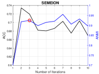
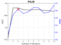
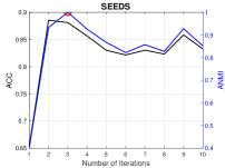
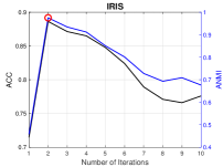
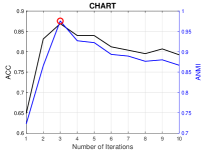
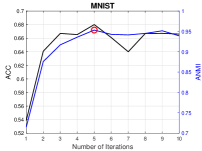
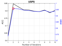
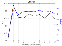
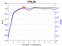
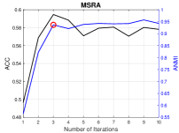
Figure 1: The black curves indicate the ACC of the proposed model against different iteration number of Algorithm 1. The blue curves draw the ANMI, i.e., the value of the proposed stopping criterion of Algorithm 1. The red circle on the blue curve indicates that the proposed stopping criterion is achieved at that point.

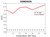
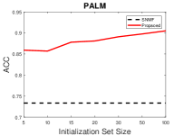
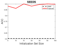
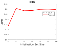
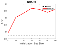
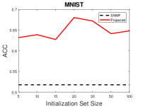
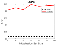
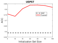
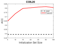
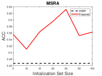
Figure 2: The ACC of the proposed model with different sizes of the initialization set on all the datasets. The black dash line refers to the ACC of SNMF as a reference.

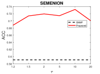
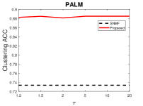
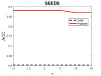
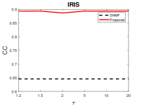
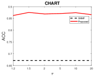
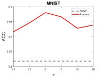
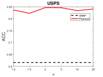
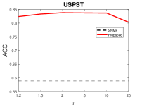
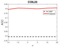
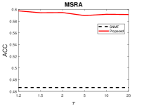
Figure 3: The influence of the value of $\tau$ on the ACC of the proposed model. We also plot the ACC of SNMF as a reference.

TABLE XII: Ablation Study of the Proposed Model

ACC	MNIST	USPST	MSRA	SEMENION	IRIS	CHART	SEEDS	USPS	PALM	COIL20	Average
SNMF	$0.518\searrow$	$0.588\searrow$	$0.467\searrow$	$0.591\searrow$	$0.645\searrow$	$0.671\searrow$	$0.602\searrow$	$0.616\searrow$	$0.733\searrow$	$0.491\searrow$	$0.592\searrow$
SOFT	$0.557\searrow$	$0.644\searrow$	$0.577\searrow$	$0.637\searrow$	$0.892\nearrow$	$0.649\searrow$	$0.653\searrow$	$0.649\searrow$	$0.846\searrow$	$0.641\searrow$	$0.674\searrow$
w/o $\bm{\alpha}$	$0.637\searrow$	$0.817\searrow$	$0.596\nearrow$	$0.726\nearrow$	$0.718\searrow$	$0.720\searrow$	$0.812\searrow$	$0.833\searrow$	$0.875\searrow$	$0.815\nearrow$	$0.755\searrow$
Proposed	$0.680$	$0.838$	$0.595$	$0.720$	$0.886$	$0.869$	$0.881$	$0.847$	$0.881$	$0.805$	0.800
NMI	MNIST	USPST	MSRA	SEMENION	IRIS	CHART	SEEDS	USPS	PALM	COIL20	Average
SNMF	$0.523\searrow$	$0.645\searrow$	$0.567\searrow$	$0.579\searrow$	$0.388\searrow$	$0.678\searrow$	$0.311\searrow$	$0.653\searrow$	$0.922\nearrow$	$0.657\searrow$	$0.592\searrow$
SOFT	$0.558\searrow$	$0.750\searrow$	$0.671\searrow$	$0.650\searrow$	$0.761\searrow$	$0.692\searrow$	$0.405\searrow$	$0.717\searrow$	$0.923\nearrow$	$0.803\searrow$	$0.693\searrow$
w/o $\bm{\alpha}$	$0.578\searrow$	$0.808\nearrow$	$0.666\searrow$	$0.672\nearrow$	$0.582\searrow$	$0.682\searrow$	$0.559\searrow$	$0.787\searrow$	$0.916\searrow$	$0.853\searrow$	$0.710\searrow$
Proposed	$0.606$	$0.805$	$0.697$	$0.667$	$0.769$	$0.828$	$0.668$	$0.794$	$0.917$	$0.857$	$0.761$
PUR	MNIST	USPST	MSRA	SEMENION	IRIS	CHART	SEEDS	USPS	PALM	COIL20	Average
SNMF	$0.569\searrow$	$0.667\searrow$	$0.502\searrow$	$0.639\searrow$	$0.664\searrow$	$0.707\searrow$	$0.616\searrow$	$0.674\searrow$	$0.793\searrow$	$0.532\searrow$	$0.636\searrow$
SOFT	$0.601\searrow$	$0.765\searrow$	$0.595\searrow$	$0.700\searrow$	$0.892\nearrow$	$0.700\searrow$	$0.672\searrow$	$0.711\searrow$	$0.877\searrow$	$0.717\searrow$	$0.723\searrow$
w/o $\bm{\alpha}$	$0.642\searrow$	$0.856\searrow$	$0.608\searrow$	$0.731\cdots$	$0.718\searrow$	$0.745\searrow$	$0.812\searrow$	$0.833\searrow$	$0.884\searrow$	$0.817\searrow$	$0.765\searrow$
Proposed	$0.684$	$0.858$	$0.629$	$0.731$	$0.886$	$0.870$	$0.881$	$0.847$	$0.886$	$0.816$	$0.809$
ARI	MNIST	USPST	MSRA	SEMENION	IRIS	CHART	SEEDS	USPS	PALM	COIL20	Average
SNMF	$0.376\searrow$	$0.488\searrow$	$0.337\searrow$	$0.435\searrow$	$0.346\searrow$	$0.557\searrow$	$0.279\searrow$	$0.505\searrow$	$0.723\searrow$	$0.386\searrow$	$0.443\searrow$
SOFT	$0.421\searrow$	$0.603\searrow$	$0.465\searrow$	$0.515\searrow$	$0.729\nearrow$	$0.573\searrow$	$0.388\searrow$	$0.594\searrow$	$0.822\searrow$	$0.573\searrow$	$0.568\searrow$
w/o $\bm{\alpha}$	$0.476\searrow$	$0.766\searrow$	$0.483\searrow$	$0.582\nearrow$	$0.508\searrow$	$0.581\searrow$	$0.552\searrow$	$0.724\searrow$	$0.850\searrow$	$0.760\cdots$	$0.628\searrow$
Proposed	$0.506$	$0.778$	$0.488$	$0.573$	$0.722$	$0.763$	$0.689$	$0.731$	$0.854$	$0.760$	$0.686$
F1-score	MNIST	USPST	MSRA	SEMENION	IRIS	CHART	SEEDS	USPS	PALM	COIL20	Average
SNMF	$0.447\searrow$	$0.546\searrow$	$0.400\searrow$	$0.497\searrow$	$0.579\searrow$	$0.641\searrow$	$0.531\searrow$	$0.560\searrow$	$0.726\searrow$	$0.421\searrow$	$0.535\searrow$
SOFT	$0.490\searrow$	$0.648\searrow$	$0.516\searrow$	$0.568\searrow$	$0.820\nearrow$	$0.656\searrow$	$0.615\searrow$	$0.641\searrow$	$0.824\searrow$	$0.600\searrow$	$0.638\searrow$
w/o $\bm{\alpha}$	$0.531\searrow$	$0.791\searrow$	$0.530\searrow$	$0.626\nearrow$	$0.673\searrow$	$0.654\searrow$	$0.704\searrow$	$0.752\searrow$	$0.851\searrow$	$0.773\cdots$	$0.688\searrow$
Proposed	$0.558$	$0.802$	$0.533$	$0.619$	$0.816$	$0.803$	$0.793$	$0.758$	$0.856$	$0.773$	$0.731$

IV-A Comparison of Clustering Performance

Tables II-XI show the clustering performance of all the methods on the 10 datasets, where the best performance under each metric is bold, and the second best is underlined. From Tables II-XI, we can observe that

• Our method significantly outperforms SNMF, especially our method improves ACC up to $0.31$ on COIL20. The improvements of our method over SNMF in terms of other metrics are also significant, e.g., the ARI increases from $0.279$ to $0.688$ on SEEDS. Moreover, the proposed method has a smaller std than SNMF on all the datasets, indicating that the proposed model is more robust to the initialization than SNMF. Note that both SNMF and the proposed method adopt the same affinity matrix as input.

• Compared with the advanced graph clustering methods, the advantage of the proposed one is also significant. For example, on CHART and USPST, our method improves the ACC $0.167$ and $0.119$, respectively, compared with the best graph clustering model. Moreover, the performance of the proposed method is also superior to that of the ensemble clustering methods. For instance, on IRIS, our method raises the ACC value from $0.720$ to $0.886$, compared with the best ensemble clustering method.

• Taking all the compared methods into account, the proposed method achieves the best performance under $44$ out of $50$ cases and the second best performance under 3 out of the remaining $6$ cases, suggesting the highly competitive clustering ability of our method.

• The performance of the compared methods is usually not robust to different datasets. For example, LWGP is good at partitioning COIL20, but not on USPST. ALS favors PALM and COIL20 more than SEMENION and CHART. vBSUM performs much better on IRIS than MSRA and COIL20. On the contrary, our method consistently produces the best or almost best performance over these 10 datasets, validating its robustness.

IV-B Influence of the Iteration Number of Algorithm 1

We studied how the number of iterations in Algorithm 1 affects clustering performance. As shown in Fig. 1, the ACC value of the proposed method increases rapidly at the first a few iterations, and then becomes relatively stable with the increase of iteration. We can also observe that on the majority datasets, the highest ACC can be selected by the proposed stopping criterion, e.g., on IRIS and MNIST. For the cases where the highest ACC is not picked, the proposed criterion can also produce a satisfied ACC for the proposed method. Besides, the proposed criterion usually terminates Algorithm 1 within $5$ iterations, which can reduce the computational cost. As a summary, the proposed stopping criterion is both effective and efficient.

IV-C Influence of the Size of the Set of Initialization

We also investigated the influence of the size of initialization set (the value of $b$) on the proposed method. Fig. 2 shows the ACC of the proposed method with the different sizes of the initialization set on all the datasets. Due to the randomness of the initialization, those curves may fluctuate at some locations. However, generally, a larger size of the initialization set leads to a higher ACC. The trend is particularly evident in COIL20, PLAM, IRIS, and CHART. Moreover, 20 different initialization are sufficient for the proposed method to achieve satisfactory performance.

IV-D Influence of the Value of $\tau$ on Performance

Here we explored the impact of the value of $\tau$ on the performance of our method. Fig. 3 shows the ACC values of our method with various $\tau$ on all the datasets, where we can find that the curves are quite flat on the majority cases, like SEEDS and COIL20. This observation demonstrates the robustness of the proposed model against $\tau$. On SEMENION and MNIST, $\tau$ should be neither too large or too small. Overall, the suggested value of $\tau$ is acceptable for all the datasets. Moreover, we also would like to emphasize that the flat curves do not dispel the importance of $\bm{\alpha}$. As will be shown in the next subsection, removing $\bm{\alpha}$ will significantly degrade the clustering performance of our model.

IV-E Ablation Study

In this section, we evaluated the importance of different components of the proposed method. Specifically, w/o $\bm{\alpha}$ denotes our model without the learable weight $\bm{\alpha}$, i.e.,

$$\begin{split}&\min_{\mathbf{V}_{m},\mathbf{S},}\sum_{m=1}^{b}\left\|\mathbf{S}-\mathbf{V}_{m}\mathbf{V}_{m}^{\mathsf{T}}\right\|_{F}^{2},~{}{\rm s.t.~{}}\mathbf{V}_{m}\geq 0,\forall m.\end{split}$$ (25)

SOFT represents the reconstruction of $\mathbf{S}$ in Eq. (7) is replaced with a soft manner, i.e.,

$$\mathbf{S}=\sum_{m=1}^{b}\alpha_{m}\mathbf{V}_{m}\mathbf{V}_{m}^{\mathsf{T}}.$$ (26)

Table XII shows the clustering performance of w/o $\bm{\alpha}$ and SOFT as well as SNMF, where $\nearrow$, $\searrow$ and $\cdots$ indicate the value of the associated metric of the compared methods is larger than, smaller than and equivalent to our S³NMF, respectively. The last column of Table XII presents the average value of each method over all the datasets. From Table XII we can observe that both SOFT and w/o $\bm{\alpha}$ are superior to SNMF but inferior to our method. Especially, according to the average values in the last column, it is obvious that our method outperforms SNMF, SOFT, and w/o $\bm{\alpha}$ to a large extent. This observation demonstrates that both the hard manner in the construction of $\mathbf{S}$ and the self-weighing scheme contribute to the proposed model. The advantage of the hard manner for constructing $\mathbf{S}$ over the soft manner is credited to that the proposed model could receive stronger feedback from the clustering result to guide the affinity matrix construction. $\bm{\alpha}$ is important because the contribution of each base SNMF can be adaptively balanced based on its quality.

V Conclusion

In this paper, by taking advantage of the characteristic that SNMF is sensitive to initialization, we have presented novel self-supervised SNMF (S³NMF) for clustering. Without relying on any additional information except multiple random nonnegative initialization matrices, our S³NMF significantly outperforms the state-of-the-art graph clustering methods and ensemble clustering methods. We formulated S³NMF as a self-weighted nonnegative constrained optimization problem, and proposed an alternating iterative optimization method to solve it and proved the convergence theoretically. Moreover, we have presented a stopping criterion to terminate the optimization process, where its effectiveness is validated by the experiments. Additionally, our model is insensitive to its hyper-parameters, and the recommended values for the hyper-parameters empirically work very well, which validate its practicability.

Appendix A

In the appendix, we prove that Eq. (16) is a valid auxiliary function of Eq. (14). The objective function of Eq. (14) can be expanded as

$$\begin{split}&(\mathbf{\alpha}_{m})^{\tau}\left\|\mathbf{S}-\mathbf{V}_{m}\mathbf{V}_{m}^{\mathsf{T}}\right\|_{F}^{2}\\ &=(\mathbf{\alpha}_{m})^{\tau}{\rm Tr}\left(\mathbf{SS}^{\mathsf{T}}-2\mathbf{SV}_{m}\mathbf{V}_{m}^{\mathsf{T}}+\mathbf{V}_{m}\mathbf{V}_{m}^{\mathsf{T}}\mathbf{V}_{m}\mathbf{V}_{m}^{\mathsf{T}}\right).\end{split}$$ (27)

The first term $\mathbf{S}\mathbf{S}^{\mathsf{T}}$ in the brackets is a constant. For the second term, we can expand it as

$$\begin{split}&{\rm Tr}\left(\mathbf{SV}_{m}\mathbf{V}_{m}^{\mathsf{T}}\right)=\sum_{i}\left(\mathbf{SV}_{m}\mathbf{V}_{m}^{\mathsf{T}}\right)_{ii}=\sum_{ijk}\mathbf{S}_{ik}\mathbf{V}_{m_{ij}}\mathbf{V}_{m_{kj}}.\end{split}$$ (28)

Since for any positive value $x$, we have $x>1+{\rm log}(x)$. Let $\frac{\mathbf{V}_{m_{ij}}\mathbf{V}_{m_{kj}}}{\mathbf{V}^{t}_{m_{ij}}\mathbf{V}^{t}_{m_{kj}}}=x$, we have:

$${\rm Tr}\left(\mathbf{SV}_{m}\mathbf{V}_{m}^{\mathsf{T}}\right)\geq\sum_{ijk}\mathbf{S}_{ik}\mathbf{V}^{t}_{m_{ij}}\mathbf{V}^{t}_{m_{kj}}\left(1+{\rm log}\frac{\mathbf{V}_{m_{ij}}\mathbf{V}_{m_{kj}}}{\mathbf{V}^{t}_{m_{ij}}\mathbf{V}^{t}_{m_{kj}}}\right).$$ (29)

For the third term, we have

$$\begin{split}&{\rm Tr}\left(\mathbf{V}_{m}\mathbf{V}_{m}^{\mathsf{T}}\mathbf{V}_{m}\mathbf{V}_{m}^{\mathsf{T}}\right)=\sum_{i}\left(\mathbf{V}_{m}\mathbf{V}_{m}^{\mathsf{T}}\mathbf{V}_{m}\mathbf{V}_{m}^{\mathsf{T}}\right)_{ii}=\\ &\sum_{ik}\left(\mathbf{V}_{m}\mathbf{V}_{m}^{\mathsf{T}}\right)_{ik}\left(\mathbf{V}_{m}\mathbf{V}_{m}^{\mathsf{T}}\right)_{ki}=\sum_{ijk}\left(\mathbf{V}_{m}\mathbf{V}_{m}^{\mathsf{T}}\right)_{ik}\mathbf{V}_{m_{kj}}\mathbf{V}_{m_{ij}}\end{split}$$ (30)

and

$${\rm Tr}\left(\mathbf{V}_{m}\mathbf{V}_{m}^{\mathsf{T}}\mathbf{V}_{m}\mathbf{V}_{m}^{\mathsf{T}}\right)\leq\sum_{ijk}\left(\mathbf{V}^{t}_{m}\mathbf{V}_{m}^{t^{\mathsf{T}}}\right)_{ik}\mathbf{V}_{m_{kj}}\frac{(\mathbf{V}_{m_{ij}})^{4}}{(\mathbf{V}_{m_{ij}}^{t})^{3}},$$ (31)

where the proof of the inequality in Eq. (31) can be found in [22]. Taking Eq. (29) and Eq. (31) into account, we have $g(\mathbf{V}_{m})\geq(\mathbf{\alpha}_{m})^{\tau}\left\|\mathbf{S}-\mathbf{V}_{m}^{t}\mathbf{V}_{m}^{t^{\mathsf{T}}}\right\|_{F}^{2}$. Moreover, when $\mathbf{V}_{m}=\mathbf{V}^{t}_{m}$, we have $g(\mathbf{V}^{t}_{m})=(\mathbf{\alpha}_{m})^{\tau}\left\|\mathbf{S}-\mathbf{V}_{m}^{t}\mathbf{V}_{m}^{t^{\mathsf{T}}}\right\|_{F}^{2}$. The two conditions in Definition 1 are satisfied, and thus $g(\mathbf{V}_{m})$ is an auxiliary function of the $\mathbf{V}_{m}$-subproblem.

References

• [1] D. D. Lee and H. S. Seung, “Algorithms for non-negative matrix factorization,” in Proc. NIPS, 2001, pp. 556–562.
• [2] ——, “Learning the parts of objects by non-negative matrix factorization,” Nature, vol. 401, no. 6755, pp. 788–791, 1999.
• [3] W. Wu, Y. Jia, S. Wang, R. Wang, H. Fan, and S. Kwong, “Positive and negative label-driven nonnegative matrix factorization,” IEEE Trans. Circuits Syst. Video Technol., pp. 1–1, 2020.
• [4] J. Choo, C. Lee, C. K. Reddy, and H. Park, “Utopian: User-driven topic modeling based on interactive nonnegative matrix factorization,” IEEE Trans. Vis. Comput. Graphics, vol. 19, no. 12, pp. 1992–2001, 2013.
• [5] J. M. Bioucas-Dias, A. Plaza, N. Dobigeon, M. Parente, Q. Du, P. Gader, and J. Chanussot, “Hyperspectral unmixing overview: Geometrical, statistical, and sparse regression-based approaches,” IEEE J. Sel. Topics Appl. Earth Observ. Remote Sens., vol. 5, no. 2, pp. 354–379, 2012.
• [6] V. Leplat, N. Gillis, and A. M. S. Ang, “Blind audio source separation with minimum-volume beta-divergence nmf,” IEEE Trans. Signal Process., pp. 1–1, 2020.
• [7] Y. Lu, Z. Lai, X. Li, D. Zhang, W. K. Wong, and C. Yuan, “Learning parts-based and global representation for image classification,” IEEE Trans. Circuits Syst. Video Technol., vol. 28, no. 12, pp. 3345–3360, 2018.
• [8] F. Liu, T. Zhou, C. Gong, K. Fu, L. Bai, and J. Yang, “Inverse nonnegative local coordinate factorization for visual tracking,” IEEE Trans. Circuits Syst. Video Technol., vol. 28, no. 8, pp. 1752–1764, 2018.
• [9] Y. Wu, B. Shen, and H. Ling, “Visual tracking via online nonnegative matrix factorization,” IEEE Trans. Circuits Syst. Video Technol., vol. 24, no. 3, pp. 374–383, 2014.
• [10] J.-X. Liu, D. Wang, Y.-L. Gao, C.-H. Zheng, Y. Xu, and J. Yu, “Regularized non-negative matrix factorization for identifying differentially expressed genes and clustering samples: A survey,” IEEE/ACM Trans. Comput. Biol. Bioinf., vol. 15, no. 3, pp. 974–987, 2017.
• [11] Y. Wang and Y. Zhang, “Nonnegative matrix factorization: A comprehensive review,” IEEE Trans. Knowl. Data Eng., vol. 25, no. 6, pp. 1336–1353, 2013.
• [12] T. Li and C.-c. Ding, “Nonnegative matrix factorizations for clustering: A survey,” in Data Clustering.   Chapman and Hall/CRC, 2018, pp. 149–176.
• [13] C.-H. Zheng, D.-S. Huang, L. Zhang, and X.-Z. Kong, “Tumor clustering using nonnegative matrix factorization with gene selection,” IEEE Trans. Inf. Technol. Biomed., vol. 13, no. 4, pp. 599–607, 2009.
• [14] W. Wu, S. Kwong, Y. Zhou, Y. Jia, and W. Gao, “Nonnegative matrix factorization with mixed hypergraph regularization for community detection,” Information Sciences, vol. 435, pp. 263–281, 2018.
• [15] D. Cai, X. He, and J. Han, “Locally consistent concept factorization for document clustering,” IEEE Trans. Knowl. Data Eng., vol. 23, no. 6, pp. 902–913, 2010.
• [16] C. Ding, X. He, and H. D. Simon, “On the equivalence of nonnegative matrix factorization and spectral clustering,” in Proc. SIAM ICDM.   SIAM, 2005, pp. 606–610.
• [17] X. Zhang, L. Zong, X. Liu, and J. Luo, “Constrained clustering with nonnegative matrix factorization,” IEEE Trans. Neural Netw. Learn. Syst., vol. 27, no. 7, pp. 1514–1526, 2016.
• [18] D. Kuang, C. Ding, and H. Park, “Symmetric nonnegative matrix factorization for graph clustering,” in Proc. SIAM ICDM.   SIAM, 2012, pp. 106–117.
• [19] D. Kuang, S. Yun, and H. Park, “Symnmf: Nonnegative low-rank approximation of a similarity matrix for graph clustering,” Journal of Global Optimization, vol. 62, no. 3, pp. 545–574, 2015.
• [20] A. Y. Ng, M. I. Jordan, and Y. Weiss, “On spectral clustering: Analysis and an algorithm,” in Proc. NIPS, 2002, pp. 849–856.
• [21] Z. Gao, N. Guan, and L. Su, “Graph regularized symmetric non-negative matrix factorization for graph clustering,” in Proc. ICDMW.   IEEE, 2018, pp. 379–384.
• [22] Y. Jia, H. Liu, J. Hou, and S. Kwong, “Clustering-aware graph construction: A joint learning perspective,” IEEE Trans. Signal Inf. Process. Netw., vol. 6, pp. 357–370, 2020.
• [23] X. Zhang, Z. Wang, L. Zong, and H. Yu, “Multi-view clustering via graph regularized symmetric nonnegative matrix factorization,” in Proc. ICCCBDA.   IEEE, 2016, pp. 109–114.
• [24] L. Yang, X. Cao, D. Jin, X. Wang, and D. Meng, “A unified semi-supervised community detection framework using latent space graph regularization,” IEEE Trans. Cybern., vol. 45, no. 11, pp. 2585–2598, 2015.
• [25] W. Wu, Y. Jia, S. Kwong, and J. Hou, “Pairwise constraint propagation-induced symmetric nonnegative matrix factorization,” IEEE Trans. Neural Netw. Learn. Syst., vol. 29, no. 12, pp. 6348–6361, 2018.
• [26] Z. Zhu, X. Li, K. Liu, and Q. Li, “Dropping symmetry for fast symmetric nonnegative matrix factorization,” in Proc. NIPS, 2018, pp. 5154–5164.
• [27] Y. Jia, H. Liu, J. Hou, and S. Kwong, “Semisupervised adaptive symmetric non-negative matrix factorization,” IEEE Trans. Cybern., pp. 1–1, 2020.
• [28] Q. Shi, H. Sun, S. Lu, M. Hong, and M. Razaviyayn, “Inexact block coordinate descent methods for symmetric nonnegative matrix factorization,” IEEE Trans. Signal Process., vol. 65, no. 22, pp. 5995–6008, 2017.
• [29] C.-G. Li, C. You, and R. Vidal, “Structured sparse subspace clustering: A joint affinity learning and subspace clustering framework,” IEEE Trans. Image Process., vol. 26, no. 6, pp. 2988–3001, 2017.
• [30] Y. Lu, Z. Lai, Y. Xu, X. Li, D. Zhang, and C. Yuan, “Nonnegative discriminant matrix factorization,” IEEE Trans. Circuits Syst. Video Technol., vol. 27, no. 7, pp. 1392–1405, 2017.
• [31] Y. Yi, J. Wang, W. Zhou, C. Zheng, J. Kong, and S. Qiao, “Non-negative matrix factorization with locality constrained adaptive graph,” IEEE Trans. Circuits Syst. Video Technol., vol. 30, no. 2, pp. 427–441, 2020.
• [32] J. Ni, H. Tong, W. Fan, and X. Zhang, “Flexible and robust multi-network clustering,” in Proc. ACM SIGKDD, 2015, pp. 835–844.
• [33] S. Al-Stouhi and C. K. Reddy, “Multi-task clustering using constrained symmetric non-negative matrix factorization,” in Proc. SIAM ICDM.   SIAM, 2014, pp. 785–793.
• [34] X. Zhang, X. Zhang, H. Liu, and J. Luo, “Multi-task clustering with model relation learning.” in Proc. IJCAI, 2018, pp. 3132–3140.
• [35] T. Shi, K. Kang, J. Choo, and C. K. Reddy, “Short-text topic modeling via non-negative matrix factorization enriched with local word-context correlations,” in Proc. WWW, 2018, pp. 1105–1114.
• [36] V. Gligorijević, Y. Panagakis, and S. Zafeiriou, “Non-negative matrix factorizations for multiplex network analysis,” IEEE Trans. Pattern Anal. Mach. Intell., vol. 41, no. 4, pp. 928–940, 2018.
• [37] M. Zhang, Z. Cui, S. Jiang, and Y. Chen, “Beyond link prediction: Predicting hyperlinks in adjacency space,” in Proc. AAAI, 2018.
• [38] M. Ganji, J. Bailey, and P. J. Stuckey, “Lagrangian constrained community detection,” in Proc. AAAI, 2018.
• [39] H. Liu, J. Wu, T. Liu, D. Tao, and Y. Fu, “Spectral ensemble clustering via weighted k-means: Theoretical and practical evidence,” IEEE Trans. Knowl. Data Eng., vol. 29, no. 5, pp. 1129–1143, 2017.
• [40] C. Lu, S. Yan, and Z. Lin, “Convex sparse spectral clustering: Single-view to multi-view,” IEEE Trans. Image Process., vol. 25, no. 6, pp. 2833–2843, 2016.
• [41] J. Huang, F. Nie, and H. Huang, “Spectral rotation versus k-means in spectral clustering,” in Proc. AAAI, 2013.
• [42] D. Huang, C. Wang, and J. Lai, “Locally weighted ensemble clustering,” IEEE Trans. Cybern., vol. 48, no. 5, pp. 1460–1473, 2018.
• [43] U. Von Luxburg, “A tutorial on spectral clustering,” Statistics and computing, vol. 17, no. 4, pp. 395–416, 2007.