An Efficient Hypergraph Approach to Robust Point Cloud Resampling

Abstract

Efficient processing and feature extraction of large-scale point clouds are important in related computer vision and cyber-physical systems. This work investigates point cloud resampling based on hypergraph signal processing (HGSP) to better explore the underlying relationship among different cloud points and to extract contour-enhanced features. Specifically, we design hypergraph spectral filters to capture multi-lateral interactions among the signal nodes of point clouds and to better preserve their surface outlines. Without the need and the computation to first construct the underlying hypergraph, our low complexity approach directly estimates hypergraph spectrum of point clouds by leveraging hypergraph stationary processes from the observed 3D coordinates. Evaluating the proposed resampling methods with several metrics, our test results validate the high efficacy of hypergraph characterization of point clouds and demonstrate the robustness of hypergraph-based resampling under noisy observations.

I Introduction

3D perception plays an important role in the high growth fields of robotics and cyber-physical systems and continues to drive many progresses made in advanced point cloud processing. 3D point clouds provide efficient exterior representation for complex objects and their surroundings. Point clouds have seen broad applications in many areas, such as computer vision, autonomous driving and robotics. Notable examples of point cloud processing include surface reconstruction [1], rendering [2], feature extraction [3], shape classification [4], and object detection/tracking [5]. When constructing point cloud of a target object, however, modern laser scan systems can generate millions of data points [6]. To achieve better storage efficiency and lower point cloud processing complexity, point cloud resampling aims to reduce the number of points in a cloud to achieve data compression while preserving the vital 3D structural and surface features. Point cloud resampling represents an important tool in various applications such as point cloud segmentation, object classification, and efficient transmission/storage. An example of point cloud resampling proposed in [7] suggested a graph-based filter to downsample point clouds and to capture the original object surface contour.

The literature already contains a variety of works on different aspects of point cloud resampling. For instance, a centroidal Voronoi tessellation method in [8] can progressively generate high-quality resampling results with isotropic or anisotropic distributions from a given point cloud to form compact representations of the underlying cloud surface. Another 3D filtering and downsampling technique [9] relies on a growing neural gas network, to deal with noise and outliers within data provided by Kinect sensors. Of particular interest is graph-based resampling approach which has exhibited desirable capability to capture the underlying structures of point clouds [10]. The graph-based method of [12] applies embedded binary trees to compress the dynamic point cloud data. Another interesting work [7] proposes several graph-based filters to capture the distribution of point data to achieve computationally efficient resampling. In addition, a contour-enhanced resampling method introduced in [11] utilizes graph-based high-pass filters.

In addition to the aforementioned class of graph-based methods, a competing class of feature-based approaches via edge detection and feature extraction has also been popular. In [13], the authors presented a sharp feature detector via Gaussian map clustering on local neighborhoods. Bazazian et al. [14] extended this principle by leveraging principal component analysis (PCA) to develop a new agglomerative clustering method. The efficiency and accuracy of this work can further benefit from spectral analysis of the covariance matrix defined by $k-$nearest neighbors. Another typical approach represented by [15] processes a noisy and possibly outlier-ridden point set in an edge-aware manner.

Both graph-based and feature-based methods have clearly achieved successes in point cloud resampling. However, some limitations remain. Graph-based methods tend to focus on pairwise relationship between different points, since each graph edge only connects two signal nodes. However, it is clear that multilateral interactions of data points could model the more informative characteristics of 3D point clouds. Bilateral graph node connections cannot even describe multilateral relationship among points on the same surface (e.g. 3 points of a triangle) directly [23]. Furthermore, in graph-based methods, efficient construction of a suitable graph to represent an arbitrary point cloud poses another challenge. Among feature-based methods, performance would vary with respect to the feature selection and filter designs. The open issues are the adequate and robust selection of features and filter parameters for practical point cloud processing.

More recently, hypergraphs have been successfully applied in representing and characterizing the underlying multilateral interactions among multimedia data points [16]. A hypergraph extends basic graph concept into higher dimensions, in which each hyperedge can connect more than two nodes [15]. Therefore for point clouds, hypergraph provides a more general representation to characterize multilateral relationship for points on object surfaces such that one hyperedge can cover multiple nodes on the same surface. Furthermore, by generalizing graph signal processing [19], hypergraph signal processing (HGSP) [21][20] provides a theoretical foundation for spectral analysis in hypergraph-based point cloud processing. Specifically, stationarity-based hypergraph estimation, in conjunction with hypergraph-based filters, has demonstrated notable successes in processing point clouds for various tasks including segmentation, sampling, and denoising [22, 23].

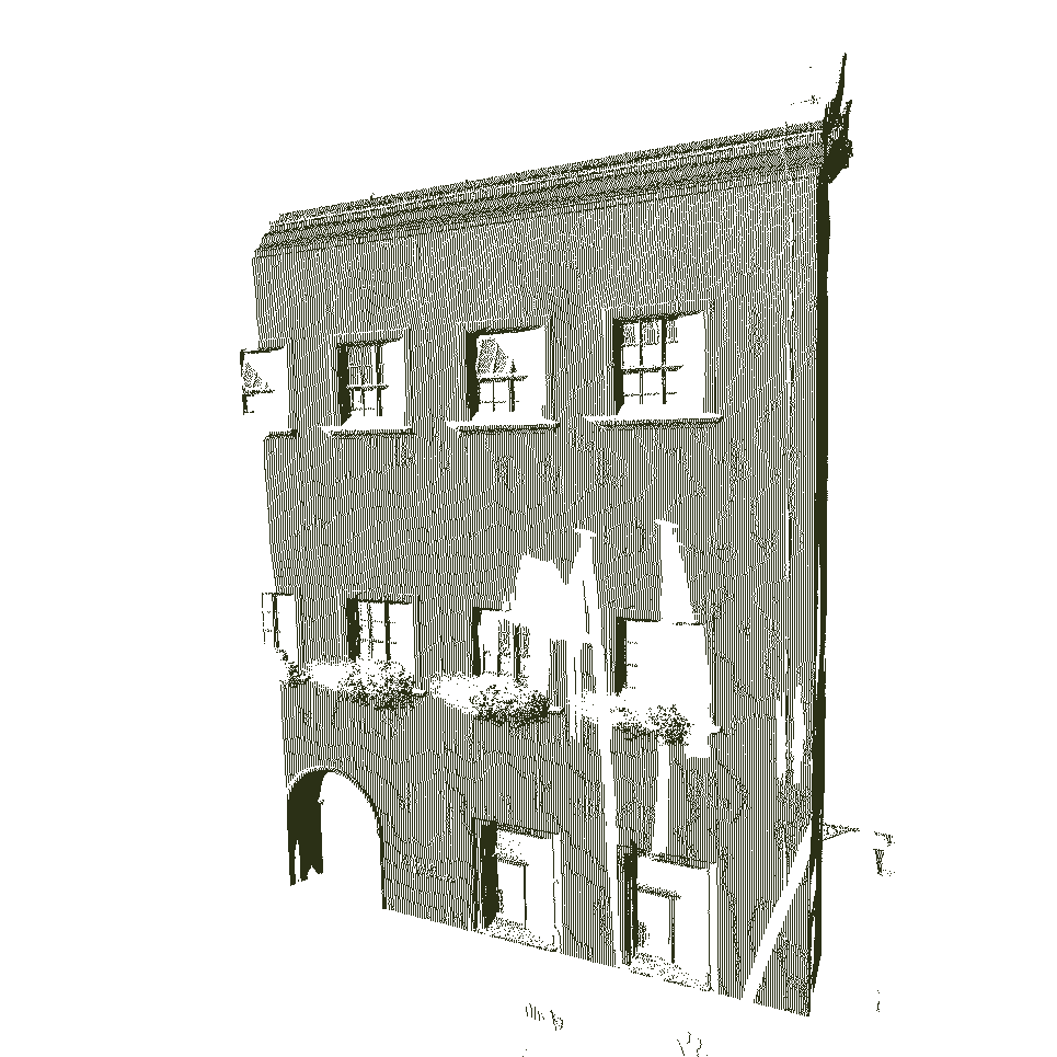
(a) Original.

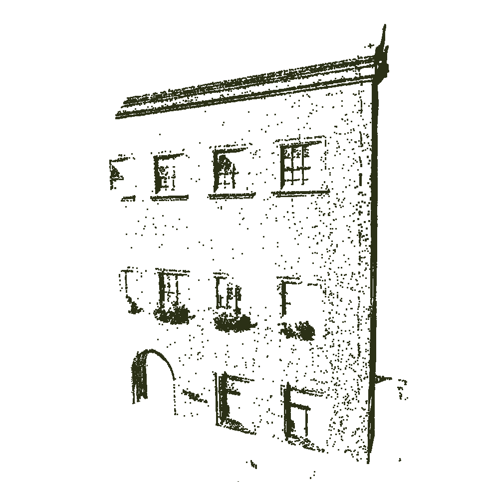
(b) Resampled.

Figure 1: Example of Contour-Enhanced Resampling: (a) original point cloud with 272705 points, and (b) resampled building based on the proposed local hypergraph filtering with 20% samples.

In this paper, we investigate point cloud resampling based on hypergraph spectral analysis. Instead of the traditional uniform resampling, we investigate contour-enhanced resampling to select subset of cloud points and to extract distinct surface features. A heuristic example is illustrated in Fig. 1 showing a point cloud successfully resampled with only 20% samples for the building. To briefly highlight the novelty of our proposed approaches, we estimate the hypergraph spectrum basis for point clouds under study by leveraging the hypergraph stationary process. We propose three novel 3D point cloud resampling methods:

• Hypergraph kernel convolution method (HKC);

• Hypergraph kernel filtering method (HKF);

• Local hypergraph filtering method (LHF).

The kernel convolution method defines a local smoothness among signals based on an operator and hypergraph convolution. The kernel filtering method defines the local smoothness with respect to high-pass filtering in spectrum domain. The local hypergraph filtering method utilizes a local sharpness definition with respect to high-pass filtering in spectrum domain. In order to test the model preserving property on complex point cloud models, we apply a simple method for point cloud recovery based on alpha complex and Poisson sampling. We then test the proposed methods under several metrics to demonstrate the compression efficiency and robustness of our proposed resampling methods with respect to the general feature preservation of point clouds under study.

We summarize the major contributions of this manuscript:

• We propose three novel hypergraph-based resampling methods to preserve distinct and sharp point cloud features;

• We provide novel definitions of hypergraph-based indicators to evaluate the smoothness or sharpness over point clouds;

• We apply different metrics to demonstrate the effectiveness of our propose methods.

We organize the rest of the manuscript as follows. Section II briefly describe basic point cloud model and introduces the fundamentals of hypergraph signal processing. We develop the foundation of HGSP based point cloud resampling and derive three new resampling methods in Section III. We provide the test results of the proposed resampling methods in Section IV, before formalizing our conclusions in Section V.

II Fundamentals and Background

II-A Point Cloud

A point cloud is a collection of points on the surface of a 3D target object. Each point consists of its 3D coordinates and may contain further features, such as colors and normals [28]. In this work, we focus on the coordinates of data points and point cloud resampling. A point cloud can be represented by the coordinates of $N$ data points written as an $N\times 3$ real-valued location matrix

$$\mathbf{P}=[\mathbf{X_{1}\quad X_{2}\quad X_{3}}]=\begin{bmatrix}\mathbf{p}_{1}^{T}\\ \mathbf{p}_{2}^{T}\\ \ddots\\ \mathbf{p}_{N}^{T}\end{bmatrix}\in\mathbb{R}^{N\times 3},$$ (1)

where $\mathbf{X}_{i}$ denotes a vector of the $i$-th coordinates of all $N$ data points whereas $3\times 1$ vector $\mathbf{p}_{i}$ indicates the $i$-th point’s coordinates.

II-B Hypergraph Signal Processing

Hypergraph signal processing (HGSP) is an analytic framework that uses hypergraph and tensor representation to model high-order signal interactions [21]. Within this framework, an $M$th-order $N$-dimensional representation tensor $\textbf{A}=(a_{i_{1}i_{2}\cdots i_{M}})\in\mathbb{R}^{N^{M}}$ models a hypergraph with $N$ vertices in each hyperedge, which is capable of connecting maximum of $M$ nodes. We may call the number of nodes connected by a hyperedge as its length. Weights of hyperedges with length less than $M$ are normalized according to combinations and permutations [18].

Orthogonal CANDECOMP/PARAFAC (CP) decomposition [24]-[26] enables the (approximate) decomposition of a representing tensor into

$$\mathbf{A}\approx\sum_{r=1}^{N}\lambda_{r}\cdot\underbrace{\mathbf{f}_{r}\circ\ldots\circ\mathbf{f}_{r}}_{M\text{ times}},$$ (2)

where $\circ$ denotes tensor outer product, $\{\mathbf{f}_{1},\cdots,\mathbf{f}_{N}\}$ are orthonormal basis to represent spectrum components, and $\lambda_{r}$ is the $r$-th spectrum coefficient corresponding to the $r$-th basis. Spectrum components {$\mathbf{f}_{1},\cdots,\mathbf{f}_{N}$} form the full hypergraph spectral space.

Similar to GSP, hypergraph signals are attributes of nodes. Intuitively, a signal is defined as $\mathbf{s}=[s_{1}\quad s_{2}\quad...\quad s_{N}]^{\mathrm{T}}\in\mathbb{R}^{N}$. Since the adjacency tensor $\mathbf{A}$ describes high-dimensional interactions of signals, we define a special form of the hypergraph signal to work with the representing tensor, i.e.,

$$\mathbf{s}^{[M-1]}=\underbrace{\mathbf{s\circ...\circ s}}_{\text{M-1 times}}.$$ (3)

Given the definitions of hypergraph spectrum and hypergraph signals, hypergraph Fourier transform (HGFT) is given by

$$\mathbf{\hat{s}}=\mathcal{F}_{C}(\mathbf{s})=[(\mathbf{f}_{1}^{\mathrm{T}}\mathbf{s})^{M-1}\cdots(\mathbf{f}_{N}^{\mathrm{T}}\mathbf{s})^{M-1}]^{\mathrm{T}}.$$ (4)

From the graph specific HGFT, hypergraph spectral convolution can be generalized [16] as

$$\mathbf{x}\diamond\mathbf{y}=\mathcal{F}_{C}^{-1}(\mathcal{F}_{C}(\mathbf{x})\odot\mathcal{F}_{C}(\mathbf{y})),$$ (5)

where $\mathcal{F}_{C}$ is the HGFT, $\mathcal{F}_{C}^{-1}$ denotes inverse HGFT (iHGFT), and $\odot$ denotes Hadamard product [21]. This definition applies the basic relationship between convolution and spectrum product, and generalizes convolution in the vertex domain into product in the hypergraph spectrum domain.

To be concise, we refrain from a full review of HGSP here. Instead, we refer readers to [21] and related works for a more extensive introduction of HGSP concepts, such as filtering, hypergraph Fourier transform, and sampling theory, among others. Equally important are concept and properties of hypergraph stationary processes which can be found in, e.g., [23].

III HGSP Point Cloud Resampling

Based on the framework of HGSP, we now develop three new edge-preserving resampling methods for point clouds: 1) kernel convolution based method, 2) kernel filtering based method, and 3) local hypergraph filtering based method.

III-A Hypergraph Kernel Convolution (HKC) based Method

In traditional image processing, kernel convolution methods such as Sobel and Prewitt [27] have achieved notable successes in edge detection. Inspired by these 2D kernel convolution methods in 2D image processing, e.g. Fig. 2(a), we define a square $k\times k\times k$ 3D cube as the slicing block to define a local signal $\mathbf{s}_{i}\in\mathbb{R}^{N_{k}}$ and a convolution kernel $\mathbf{G}\in\mathbb{R}^{N_{k}}$ with $N_{k}=k^{3}$ aimed at extracting sharp outliers of the point cloud under study. An example of $3^{3}$ cubic 3D convolution kernel is shown in Fig. 2(b). Note that the hypergraph convolution kernel can assume different shapes and sizes depending on the datasets.

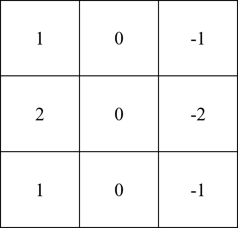
(a) 2D Sobel Kernel.

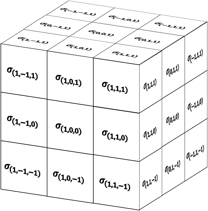
(b) 3D Hypergraph Kernel.

Figure 2: Example of Convolution Kernels.

For the $i$-th point in an original point cloud, its corresponding local signal $\mathbf{s}_{i}\in\mathbb{R}^{N_{k}}$ is defined according to the number of points in the voxel of kernel centered at $i$-th point. An example of the local signal is shown in Fig. 3. Although the idea behind the use of, e.g., 3D sobel operator is straightforward, technical obstacles arise mainly due to two reasons: (1) nodes in 3D point cloud are not always on grid; (2) two signals in graph/hypergraph based convolution must have the same length. Thus, we let $N_{k}$ be equal to the number of voxels in the kernel. Let $d$ be the distance between the centers of two nearby voxels in the kernel. A proper selection of $d$ should allow $\mathbf{s}_{i}$ to capture the local geometric information. If $d$ is too small, only a few neighbors of $i$-th point are included in the $\mathbf{s}_{i}$ and it is sensitive to measurement noise; If $d$ is too large, large number of neighbors are included in each voxel, which may lead to the blurring of detailed local geometric information. We choose $d$ to be the intrinsic resolution of a point cloud.

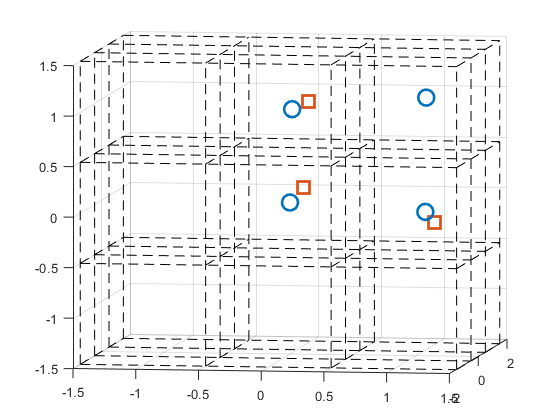
Figure 3: An example of local signal $\mathbf{s}_{i}$: Points in the middle layer are marked by blue circles and points in the back layer are marked by red squares. The voxels of slicing block are delineated by the dash black lines. There is at most one point in each voxel in this example, such that $\mathbf{s}_{i}(n)=1$ or 0, respectively, depending on whether or not the $n$-th voxel contains a point.

Given the definition of signals, we now propose a new hypergraph convolution based method. Our kernel convolution based method consists of two main steps: i) hypergraph spectrum estimation, and ii) kernel convolution using hypergraph spectrum.

We first estimate the hypergraph spectrum based on hypergraph stationary process. Introduced in [23], a stochastic signal $\mathbf{x}$ is weak-sense hypergraph stationary if and only if it has zero-mean and its covariance matrix has the same eigenvectors as the hypergraph spectrum basis, i.e.,

$$\mathbb{E}[\mathbf{x}]=\mathbf{0},$$ (6)

and

$$\mathbb{E}[\mathbf{x}\mathbf{x}^{H}]=\mathbf{V}\Sigma_{\mathbf{x}}\mathbf{V}^{H},$$ (7)

where $\mathbf{V}$ is the hypergraph spectrum basis. Since the 3D coordinates can be viewed as three observations of the point cloud from different projection directions, we can estimate the hypergraph spectrum from the covariance matrix of three coordinates based on assumption of signal stationarity. Here, we use the same spectrum estimation strategy as [23], and consider the adjacency tensor as a third-order tensor, which is the minimum number of nodes to form a surface.

III-A1 HKC Algorithm

Let $\mathbf{P_{c}}=[\mathbf{X_{1}}\ \mathbf{X_{2}}\ \mathbf{X_{3}}]\in\mathbb{R}^{N_{k}\times 3}$ be the coordinates of the total $N_{k}$ voxel centers in the kernel. For our $3\times 3\times 3$ kernel example, $N_{k}=27$. We then normalize the coordinates $\mathbf{P_{c}}$ to obtain a zero mean signal $\mathbf{P^{\prime}_{c}}$. By calculating the eigenvectors {$\mathbf{f}_{1},\cdots,\mathbf{f}_{N_{k}}$} for $R_{\mathbf{P^{\prime}_{c}}}=\mathbf{P^{\prime}_{c}}\mathbf{P^{\prime}_{c}}^{T}$, we can estimate the hypergraph spectrum basis $\mathbf{V}=[\mathbf{f}_{1},\cdots,\mathbf{f}_{N_{k}}]$.

Next, we implement convolution between the local signal $\mathbf{s}_{i}$ and the kernel $\mathbf{G}$. Since we consider the third-order tensor and are only interested in signal energies in the spectrum domain, we can utilize the hypergraph spectrum to calculate a simplified-form of HGFT $\hat{\mathbf{s}}_{i}$ and a corresponding inverse HGFT (iHGFT) of original signals $\mathbf{s}_{i}$, instead of the HGFT and iHGFT of the hypergraph signal $\mathbf{s}_{i}^{[M-1]}$ in Eq. (4).

Recall from [21] that simplified HGFT and iHGFT of original signal can are, respectively,

$$\mathcal{F}(\mathbf{s}_{i}) =\hat{\mathbf{s}}_{i}=\mathbf{V}^{H}\mathbf{s}_{i},$$ (8)

$$\mathcal{F}^{-1}(\hat{\mathbf{s}}_{i}) =\mathbf{s}_{i}=\mathbf{V}\hat{\mathbf{s}}_{i}.$$ (9)

Note that the hypergraph signal is an $(M-1)$-fold tensor outer product of the original signal in vertex domain, corresponding to $(M-1)$-fold Hadamard product in spectrum domain, where they share the same bandwidth.

Algorithm 1 Hypergraph Kernel Convolution (HKC)

  Input: A point cloud of $N$ nodes with coordinates $\mathbf{P}=[\mathbf{p}_{1}^{T}\cdots\mathbf{p}_{N}^{T}]^{T}$, resampling ratio $\alpha$.

  1. Calculate the intrinsic resolution of point cloud;

  2. Use intrinsic resolution $d$ to find coordinates $\mathbf{P_{c}}\in\mathbb{R}^{N_{k}\times 3}$ of voxel centers in the kernel;

  3. Use the coordinates $\mathbf{P_{c}}$ of voxel centers in the kernel to estimate the hypergraph spectrum basis $\mathbf{V}=[\mathbf{f}_{1},\cdots,\mathbf{f}_{N_{k}}]$ and corresponding eigenvalues $\bm{\lambda}$;

  for $i=1,2,\cdots,N$ do

     4. Use hypergraph spectrum basis $\mathbf{V}$ to calculate the Fourier transform $\hat{\mathbf{s}}_{i}$ in Eq. (8);

     5. Calculate the Hadamard product $\hat{\mathbf{s}}_{oi}=\hat{\mathbf{s}}_{i}\odot\hat{\mathbf{G}}$;

     6. Calculate inverse Fourier transform $\mathbf{s}_{oi}$ using Eq. (9);

     7. Calculate local smoothness $\beta_{i}$ in Eq. (11) ;

  end for

  8. Sort the local smoothness $\beta_{i}$ in descending order and select the bottom $N_{r}=\alpha N$ nodes as the resampled point cloud.

Directly designing convolution kernel $\mathbf{G}$ in vertex domain is challenging for two main reasons. First, since hypergraph spectrum basis $\mathbf{V}$ would vary for different kernels, finding a general $\mathbf{G}$ in vertex domain that performs equally well for various different bases would be difficult. Second, since the convolution result $\mathbf{s}_{oi}$ between the signal $\mathbf{s}_{i}$ and the kernel $\mathbf{G}$ can be expressed as

$$\mathbf{s}_{oi} =\mathbf{V}(\hat{\mathbf{G}}\odot\hat{\mathbf{s}}_{i})$$

$$=\mathbf{V}\bigl{(}diag(\hat{\mathbf{G}})\hat{\mathbf{s}}_{i}\bigr{)}$$

$$=\mathbf{V}diag(\hat{\mathbf{G}})\mathbf{V}^{H}\mathbf{s}_{i},$$ (10)

it is convenient to design spectrum domain $\hat{\mathbf{G}}$ directly.

In order to preserve edges in the resampled point cloud, we use a highpass filter defined in spectrum domain. Here, we use a Haar-like highpass design i.e., $\hat{\mathbf{G}}=\mathbf{1}-\bm{\lambda}$, where $\bm{\lambda}=[\lambda_{1}\ \lambda_{2}\cdots\lambda_{N_{k}}]^{T}$ are eigenvalues corresponding to eigenvectors {$\mathbf{f}_{1},\cdots,\mathbf{f}_{N_{k}}$}, respectively. We use the ratio between the norm of the convolution output $\mathbf{s}_{oi}$ and the norm of $\mathbf{s}_{i}-\mathbf{s}_{oi}$ to measure smoothness $\beta_{i}$ for the $i$-th point, i.e.,

$$\beta_{i}=\frac{\|\mathbf{s}_{oi}\|}{\|\mathbf{s}_{i}-\mathbf{s}_{oi}\|}.$$ (11)

In resampling, we would like to extract distinct and sharp features by selecting points that exhibit lower $\beta_{i}$ value from the resampling output. Our algorithm is summarized as Algorithm 1, also known as the HKC resampling algorithm.

III-A2 Complexity Analysis

In an unorganized point cloud, the computational complexity order for generating $\mathbf{s}_{i}$ of all points is ${O}(N^{2})$. This is because we would have to search the point cloud to find actual neighbors for each data point. To compute the estimated hypergraph spectrum basis $\mathbf{V}$ and $\mathbf{V}^{H}$ requires finding eigenvectors of $R_{\mathbf{P^{\prime}_{c}}}$ which has computational complexity of $O(N_{k}^{3})$. The cost of computing all HGFT and iHGFT pairs equals $O(NN_{k}^{2})$. The total complexity of computing $\beta_{i}$ in Eq. (11) would be $O(NN_{k})$ and it further requires ${O}(N\log{N})$ steps to sort the $\beta_{i}$s. The computational complexity of the HKC algorithm amounts to $O(N^{2}+N\log{N}+N_{k}(N_{k}+1)N+N_{k}^{3})$. In an organized point cloud, the computational complexity of generating $\mathbf{s}_{i}$ for all points can be reduced to ${O}(N)$, such that the computational complexity of the HKC resampling is only $O(N\log{N}+(N_{k}^{2}+N_{k}+1)N+N_{k}^{3})$.

III-B Hypergraph Kernel Filtering (HKF) Resampling

To present method, we still use the $3\times 3\times 3$ cube as the example kernel, and the same local signal $\mathbf{s}_{i}$ in the Kernel convolution based method.

III-B1 HKF Resampling

Consider convolution via Hadamard product and inverse Fourier transform in the HKC resampling algorithm. We need to transform the local signal $\mathbf{s}_{i}$ from vertex domain to spectrum domain. A simpler alternative is to compute local smoothness directly for signals in spectrum domain. The computational complexity of the algorithm is reduced by eliminating the inverse transform.

For edge-preserving, we wish to separate the high frequency coefficients from the low frequency coefficients in spectrum domain. Recall that the spectrum bases corresponding to smaller $\lambda$ represent higher frequency components [21]. Thus, we sort the eigenvalues of $R_{\mathbf{s^{\prime}}}$ as $0\leq\lambda_{1}\leq\lambda_{2}\leq\ldots\leq\lambda_{N_{k}}$ with corresponding eigenvectors {$\mathbf{f}_{1},\cdots,\mathbf{f}_{N_{k}}$}. We can devise a threshold $\theta$ to separate the high frequency components from the low frequency components according to a sharp rise of successive eigenvalues.

Algorithm 2 Hypergraph Kernel Filtering (HKF)

  Input: A point cloud with $N$ nodes characterized by $\mathbf{P}=[\mathbf{p}_{1}^{T}\cdots\mathbf{p}_{N}^{T}]^{T}$, resampling ratio $\alpha$.

  1. Calculate the intrinsic resolution of point cloud;

  2. Use the intrinsic resolution as $d$ to get the coordinates $\mathbf{P_{c}}\in\mathbb{R}^{N_{k}\times 3}$ of voxel centers in the kernel;

  3. Use the coordinates $\mathbf{P_{c}}$ of the voxel centers in the kernel to estimate the hypergraph spectrum basis $\mathbf{V}=[\mathbf{f}_{1},\cdots,\mathbf{f}_{N_{k}}]$;

  for $i=1,2,\cdots,N$ do

     4. Use hypergraph spectrum basis $\mathbf{V}$ to calculate the Fourier transform $\hat{\mathbf{s}}_{i}$ in Eq. (8);

     5. Calculate the local smoothness $\sigma_{i}$ in Eq. (12);

  end for

  6. Sort the local smoothness $\sigma_{i}$ and select the bottom $N_{r}=\alpha N$ points as the resampled point cloud.

Given a threshold selection of $\theta$, we could further define a local smoothness $\sigma_{i}$ to select the resampled points:

$${\sigma_{i}=\frac{\sum_{k\in\{1,2,\cdots,\theta\}}|\hat{\mathbf{s}}_{i}(k)|}{\sum_{k\in\{1,2,\cdots,{N_{k}}\}}|\hat{\mathbf{s}}_{i}(k)|}},$$ (12)

which is the fraction of high frequency energy within total signal energy.

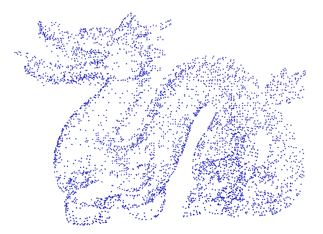
(a) Resampled results of “dragon” using local hypergraph filtering based method with signal length $N_{i}=3$. Details in the body part are kept.

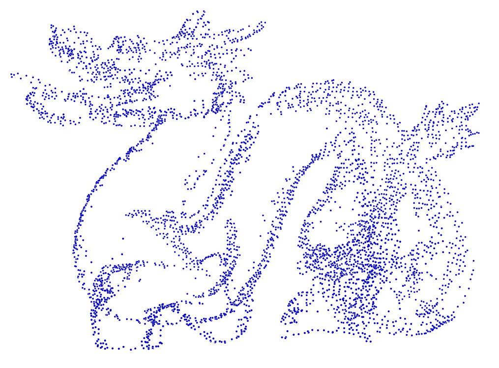
(b) Resampled results of “dragon” using local hypergraph filtering based method with signal length $N_{i}=6$. Details in the body part are ignored.

Figure 4: Resampled Results of Dragon Using Local Hypergraph Filtering based Method.

Finally, we resample the point cloud by selecting the points with smaller $\sigma_{i}$, which correspond to points containing larger amount of higher-frequency components in the hypergraph. We summarize our algorithm as Algorithm 2, also known as HKF resampling algorithm. Since the resampled point clouds favor high-frequency points, they tend to contain more sharp features and are less smooth.

III-B2 HKF Algorithm Complexity

Similar to HKC resampling, for an unorganized point cloud, the computational complexity for generating $\mathbf{s}_{i}$ for all points is ${O}(N^{2})$. To estimate the hypergraph spectrum basis $\mathbf{V}$ and $\mathbf{V}^{H}$, the complexity is $O(N_{k}^{3})$. The cost of computing requisite Fourier transforms amounts to $O(NN_{k}^{2})$. The total complexity of computing $\beta_{i}$ in Eq. (12) is $O(NN_{k})$. It further requires ${O}(N\log{N})$ to sort the $\{\sigma_{i}\}$. In summary, the computational complexity of Algorithm 2 (HKF algorithm) is $O(N^{2}+N\log{N}+N_{k}(N_{k}+1)N+N_{k}^{3})$. For an organized point cloud, however, the computational complexity for generating $\mathbf{s}_{i}$ for all points is reduced to ${O}(N)$, such that the computational complexity of HKF is reduced to $O(N\log{N}+(N_{k}^{2}+N_{k}+1)N+N_{k}^{3})$.

III-C Local Hypergraph Filtering (LHF) Algorithm

We further propose another novel HGSP approach to model the local signal by incorporating the vector between the $i$-th point and each of its ($N_{i}-1$) closest neighbors. In particular, we define a local signal for the $i$-th node of order $N_{i}$ as

$$\mathbf{s}_{p,i}=[\mathbf{0}^{T}\ (\mathbf{p_{n_{1}}}-\mathbf{p_{i}})^{T}\cdots(\mathbf{p_{n_{N_{i}-1}}}-\mathbf{p_{i}})^{T}]^{T}\in\mathbb{R}^{N_{i}\times 3},$$ (13)

where $n_{1},\cdots,n_{N_{i}-1}$ are the indices of its ($N_{i}-1$) nearest neighbors.

We then build hypergraphs over these cloud points and use hyperedge to connect point $i$ and its ($N_{i}-1$) nearest neighbors. Similar to the HKF algorithm, we also devise a filter defined in spectrum domain to process the local signal. Although, strictly speaking, we could define a unique $N_{i}$ for each of the $i$-th point, we find it more convenient to consider some fixed selections for all points to avoid comparing hyperedges of different length.

Fig. 4 provides an example to show the effect of $N_{i}$ selection. When $N_{i}$ is small, $\mathbf{s}_{p,i}$ describes the local geometric information in a smaller region. Consequently, the filtered results tend to vary more and captures sharp features of the point cloud in Fig. 4(a). When $N_{i}$ is large, $\mathbf{s}_{p,i}$ characterize the local geometry of a larger region around the $i$-th point. As a result, its local information is blurred with other local information from its neighbors such that the filtered results tend to be smoother and tend to highlight the contour of the point cloud as seen from Fig. 4(b).

III-C1 Local Hypergraph Filtering (LHF) Resampling

Because we would like to preserve both the sharp features and the surface contour of the point cloud to achieve consistently good performance across different point clouds, we propose to apply several values of $N_{i}$ for all points. In particular, we consider two different lengths $N_{a},N_{b}$ to construct two different sets of local signals. We would then integrate the filtered results.

Our local hypergraph filtering (LHF) based resampling consists of two main steps: i) hypergraph spectrum construction, ii) spectrum domain filtering. We first estimate hypergraph spectrum by applying the same process used in HKC and HKF algorithms. In this new LHF method, each cloud point has its own (small-scale) hypergraph. We should estimate the hypergraph spectrum for each point using two different local signals $\mathbf{s}_{p,i,a}\in\mathbb{R}^{N_{a}\times 3}$ and $\mathbf{s}_{p,i,b}\in\mathbb{R}^{N_{b}\times 3}$. Once the estimation of the corresponding hypergraph spectrum bases $\mathbf{V}_{i,a}$ and $\mathbf{V}_{i,b}$ is completed, we apply Eq. (8) to derive the Fourier transform $\hat{\mathbf{s}}_{p,i,a}$ and $\hat{\mathbf{s}}_{p,i,b}$, respectively.

Similar to spectrum filter in the HKF method, we define two thresholds $\theta_{i,a}$ and $\theta_{i,b}$, respectively, for $\hat{\mathbf{s}}_{p,i,a}$ and $\hat{\mathbf{s}}_{p,i,b}$. Two local sharpness metrics are further defined as

$$\gamma(\hat{\mathbf{s}}_{p,i,a}) =\frac{\sum_{j\in\{1,2,\cdots,\theta_{i,a}\}}\sum_{k=1}^{3}|\hat{\mathbf{s}}_{p,i,a}(j,k)|}{\sum_{j\in\{1,2,\cdots,N_{i}\}}\sum_{k=1}^{3}|\hat{\mathbf{s}}_{p,i,a}(j,k)|},$$ (14a)

$$\gamma(\hat{\mathbf{s}}_{p,i,b}) =\frac{\sum_{j\in\{1,2,\cdots,\theta_{i,b}\}}\sum_{k=1}^{3}|\hat{\mathbf{s}}_{p,i,b}(j,k)|}{\sum_{j\in\{1,2,\cdots,N_{i}\}}\sum_{k=1}^{3}|\hat{\mathbf{s}}_{p,i,b}(j,k)|},$$ (14b)

where $\theta_{i,a}$ and $\theta_{i,b}$ correspond to the thresholds for $\hat{\mathbf{s}}_{p,i,a}$ and $\hat{\mathbf{s}}_{p,i,b}$, respectively, with $N_{a}$ and $N_{b}$ as the respective corresponding lengths.

Upon completion of sharpness evaluation, for each signal point, we apply a weighted average of $\gamma(\hat{\mathbf{s}}_{p,i,a})$ and $\gamma(\hat{\mathbf{s}}_{p,i,b})$ to form a combined sharpness result

$$\gamma_{i}=\epsilon\gamma(\hat{\mathbf{s}}_{p,i,a})+(1-\epsilon)\gamma(\hat{\mathbf{s}}_{p,i,b}),$$ (15)

where $\epsilon$ denotes the weight.

To balance the effect of two local sharpness metrics, we sort both $\gamma(\hat{\mathbf{s}}_{p,i,a})$ and $\gamma(\hat{\mathbf{s}}_{p,i,b})$ and design the weight $\epsilon$ according to the top $\alpha$ fraction of $\gamma(\hat{\mathbf{s}}_{p,i,a})$ and $\gamma(\hat{\mathbf{s}}_{p,i,b})$, denoted by $\Gamma_{a}$ and $\Gamma_{b}$, respectively. We can define node-specific weights

$$\epsilon=\frac{\Gamma_{b}}{\Gamma_{a}+\Gamma_{b}}.$$ (16)

Finally, we sort the $\gamma_{i}$ of Eq. (15) and select the top $N_{\alpha}=\alpha N$ points as the resampled point cloud. The whole algorithm is summarized as Algorithm 3, also known as the LHF algorithm.

III-C2 LHF Algorithm Complexity

Given an unorganized point cloud, the computational complexity for generating $\mathbf{s}_{p,i}$ for all points is ${O}(N^{2})$. To estimate the hypergraph spectrum bases $\mathbf{V}_{i,a}$s and $\mathbf{V}_{i,b}$s, the computational complexity will be $O(NN_{k}^{3})$. The cost of computing all the Fourier transforms and inverse Fourier transforms amounts to $O(NN_{k}^{2})$. The total complexity of computing $\gamma_{i}$ is $O(NN_{k})$. It further requires ${O}(N\log{N})$ computations to sort all $\gamma_{i}$. The computational complexity of the LHF Algorithm is $O(N^{2}+N\log{N}+N_{k}(N_{k}^{2}+N_{k}+1)N)$. Given an organized point cloud, the computational complexity of generating $\mathbf{s}_{p,i}$ for all points is reduced to ${O}(N)$. Thus, the overall computational complexity of LHF algorithm reduces to $O(N\log{N}+(N_{k}^{3}+N_{k}^{2}+N_{k}+1)N)$.

Algorithm 3 Local Hypergraph Filtering (LHF) Resampling

  Input: A point cloud with $N$ nodes characterized by $\mathbf{P}=[\mathbf{p}_{1}^{T}\cdots\mathbf{p}_{N}^{T}]^{T}$, resampling ratio $\alpha$, local lengths $N_{a},N_{b}$.

  for $i=1,2,\cdots,N$ do

     1. Find the nearest ($N_{a}-1$) and ($N_{b}-1$) neighbors of point $i$;

     2. Use coordinates of point $i$ and its ($N_{a}-1$) and ($N_{b}-1$) neighbors to estimate the hypergraph spectrum bases $\mathbf{V}_{i,a}$, $\mathbf{V}_{i,b}$, respectively;

     3. Use hypergraph spectrum basis $\mathbf{V}_{i,a}$ and $\mathbf{V}_{i,b}$ to calculate the Fourier transform $\hat{\mathbf{s}}_{p,i,a}$ and $\hat{\mathbf{s}}_{p,i,b}$, respectively;

     4. Calculate the local sharpness $\gamma(\hat{\mathbf{s}}_{p,i,a})$ and $\gamma(\hat{\mathbf{s}}_{p,i,b})$ in Eq. (14a) and Eq. (14b);

  end for

  5. Calculate the weighted average of $\gamma_{i}(\hat{\mathbf{s}}_{p,i,a})$ and $\gamma_{i}(\hat{\mathbf{s}}_{p,i,b})$ using Eq. (15) and Eq. (16).

  6. Sort the local sharpness $\gamma_{i}$ and select the top $N_{r}=\alpha N$ points as the resampled point cloud.

IV Experimental results

	HKC				HKF
Noise Level	Precision	Recall	F1-Score	Mean Distance	Precision	Recall	F1-Score	Mean Distance
No noise	0.3810	0.9957	0.5497	0.6285	0.3652	0.9585	0.5276	0.6442
10%	0.3801	0.9934	0.5485	0.7322	0.3501	0.9199	0.5060	1.1475
20%	0.2560	0.6709	0.3697	2.5501	0.1499	0.3913	0.2163	3.7606

	LHF				GFR
Noise Level	Precision	Recall	F1-Score	Mean Distance	Precision	Recall	F1-Score	Mean Distance
No noise	0.3578	0.9371	0.5166	1.0376	0.3827	1	0.5522	0.4516
10%	0.1437	0.3763	0.2075	2.4587	0.3818	0.9978	0.5509	2.9787
20%	0.0899	0.2358	0.1299	3.4143	0.2312	0.6050	0.3337	3.9326

	EA				PCA-AC
Noise Level	Precision	Recall	F1-Score	Mean Distance	Precision	Recall	F1-Score	Mean Distance
No noise	0.3827	1	0.5522	1.0393	0.3752	0.9825	0.5418	0.8292
10%	0.3785	0.9902	0.5463	0.9792	0.3539	0.9318	0.5117	0.7424
20%	0.3597	0.9421	0.5193	1.2916	0.3418	0.8988	0.4941	0.9367

TABLE I: Numerical results of methods for edge preserving resampling without and with Gaussian noise.

We now describe our experiment setup and present test results of the three proposed new resampling algorithms.

IV-A Edge Preservation of Simple Synthetic Point Clouds

As we described in Section III, one important resampling objective is to preserve sharp features in a point cloud such as edges and corners. In this part, we study the edge preserving capability of our proposed algorithms by testing over several simple synthetic point clouds. The reason for selecting synthetic point clouds in this test is to take advantage of the known ground truth regarding edges and our ability to label them. We generate these synthetic point clouds by uniformly sampling the external surface of models constructed from combinations of cubes of various sizes. One example of synthetic point clouds is shown in Fig. 5, where the points on edges are marked in red while the remaining points are in blue.

To measure the accuracy of the preserved edges, we evaluate the $F_{1}$ score, defined by

$$F_{1}=2\cdot\frac{\rm{Precision}\cdot\rm{Recall}}{\rm{Precision}+\rm{Recall}},$$ (17)

where precision denotes the fraction of edge points correctly preserved among all (false or correct) edge points for a resampling algorithm while the recall is the ratio of correctly preserved edge points versus all ground truth edge points. We also calculate the mean distance to their closest ground truth edge point respectively to show the ability of the algorithms in capturing the model surface.

For baseline comparison, we also test the graph-based fast resampling (GFR) method of [7] on the same datasets. We also compare with an edge detection method based on eigenvalues analysis (EA) and another edge detection algorithm based on Principal Component Analysis (PCA) and agglomerative clustering (PCA-AC) [14]. The parameters of GFR method are set to the typical values suggested by [7]. For EA and PCA-AC, we retain the points with higher cluster numbers or larger surface variation in the resampled point cloud to yield the same resampling ratio. Here, we set the resampling ratio $\alpha=0.2$ for all point clouds as an example. additional results with different resampling ratios will be further presented in Section IV-C. In order to study the robustness of algorithms, we also add 10% and 20% of Normal measurement noises to the coordinates of point cloud, respectively. Table I summarizes our test results.

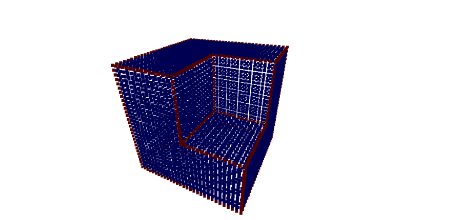
Figure 5: A Synthetic Point Cloud with Labeled Edge.

Compared with the GSP based GFR method, the newly proposed hypergraph kernel convolution (HKC) algorithm performs robustly for point clouds under larger measurement noises. Since the local signals in HKC are defined by the number of points in the voxel of kernel, weaker noises on a single point with perturbation below $d$/2 (the intrinsic resolution of original point clouds) would not affect local signals.

On the other hand, LHF algorithm does not perform well against noisy point clouds because sizable noises directly distort the local hypergraph and neighbors. Overall, our proposed HGSP-based methods demonstrate stronger robustness than the traditional graph-based GFR algorithm for noisy data. Using a generic signal processing approach they also deliver competitive performance against non-graph based EA and PCA-AC methods that were designed specifically for edge detection.

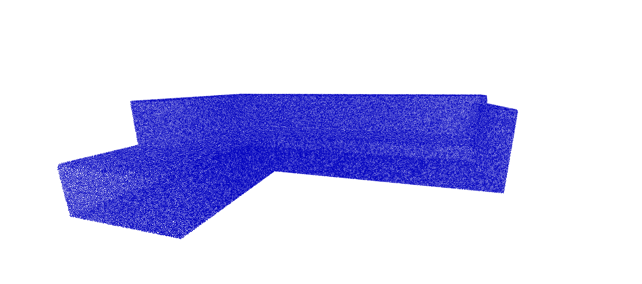
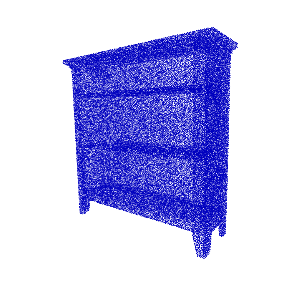
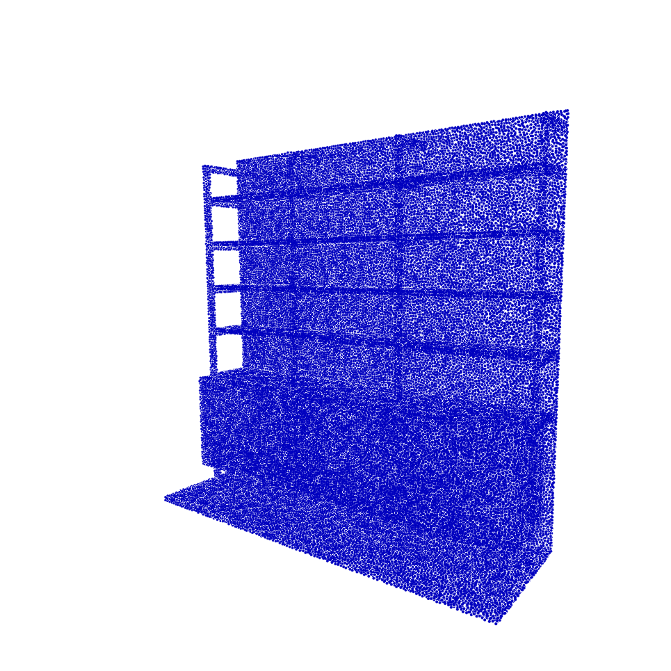
(a) Original Point Clouds

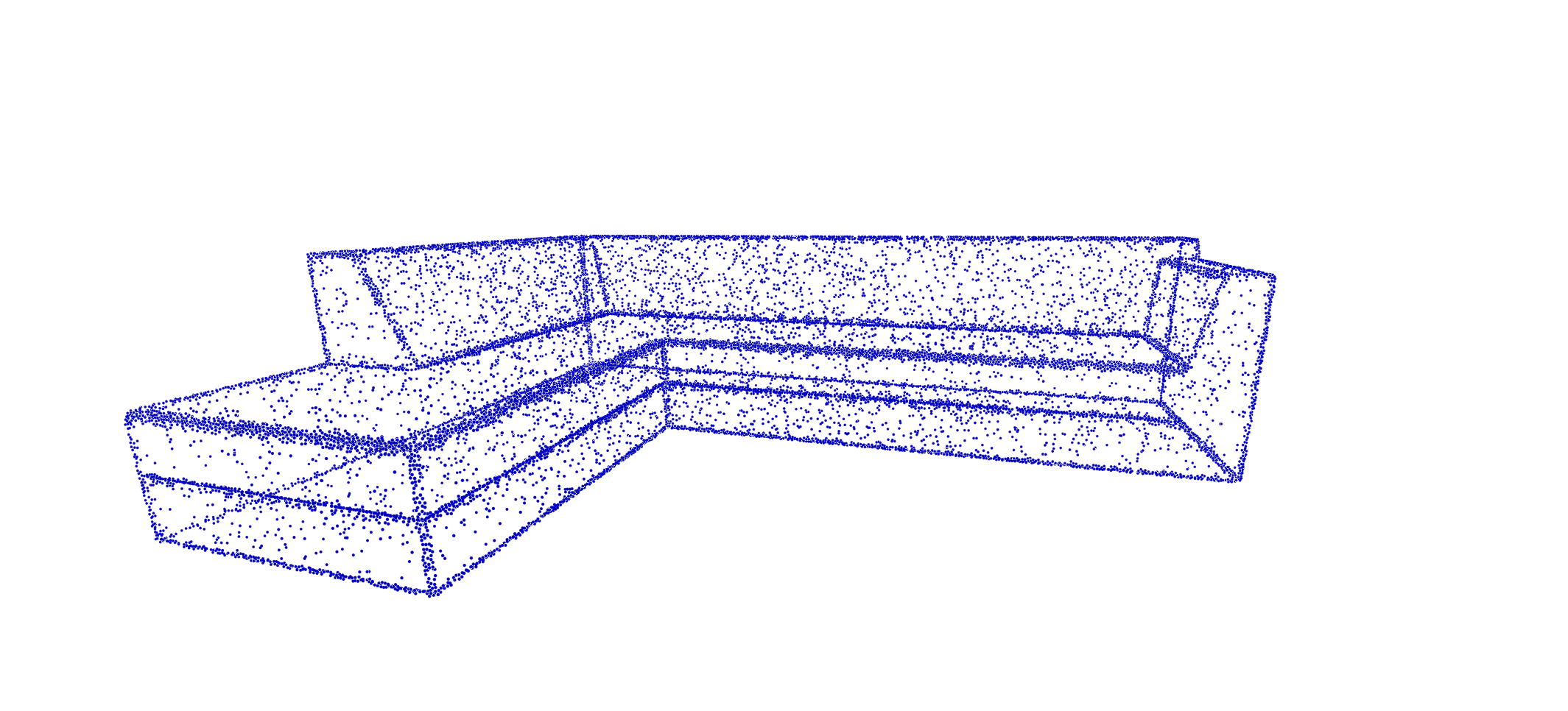
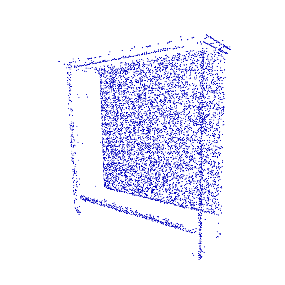
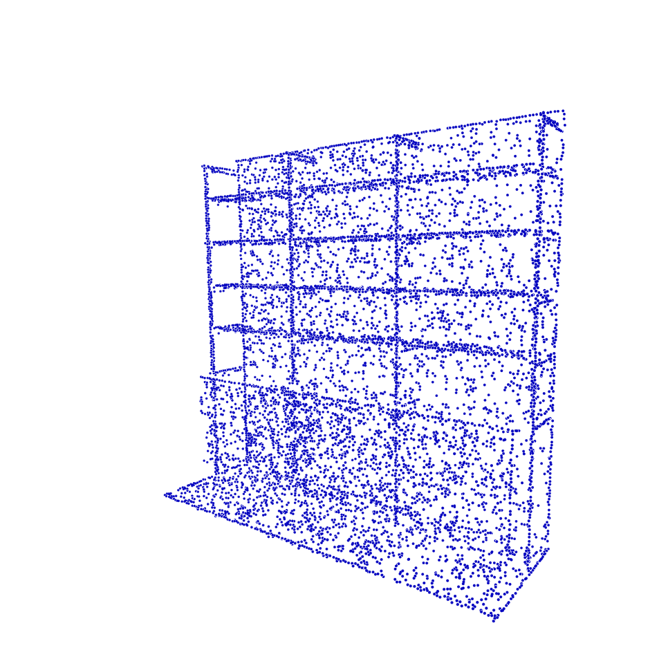
(b) Hypergraph Convolution

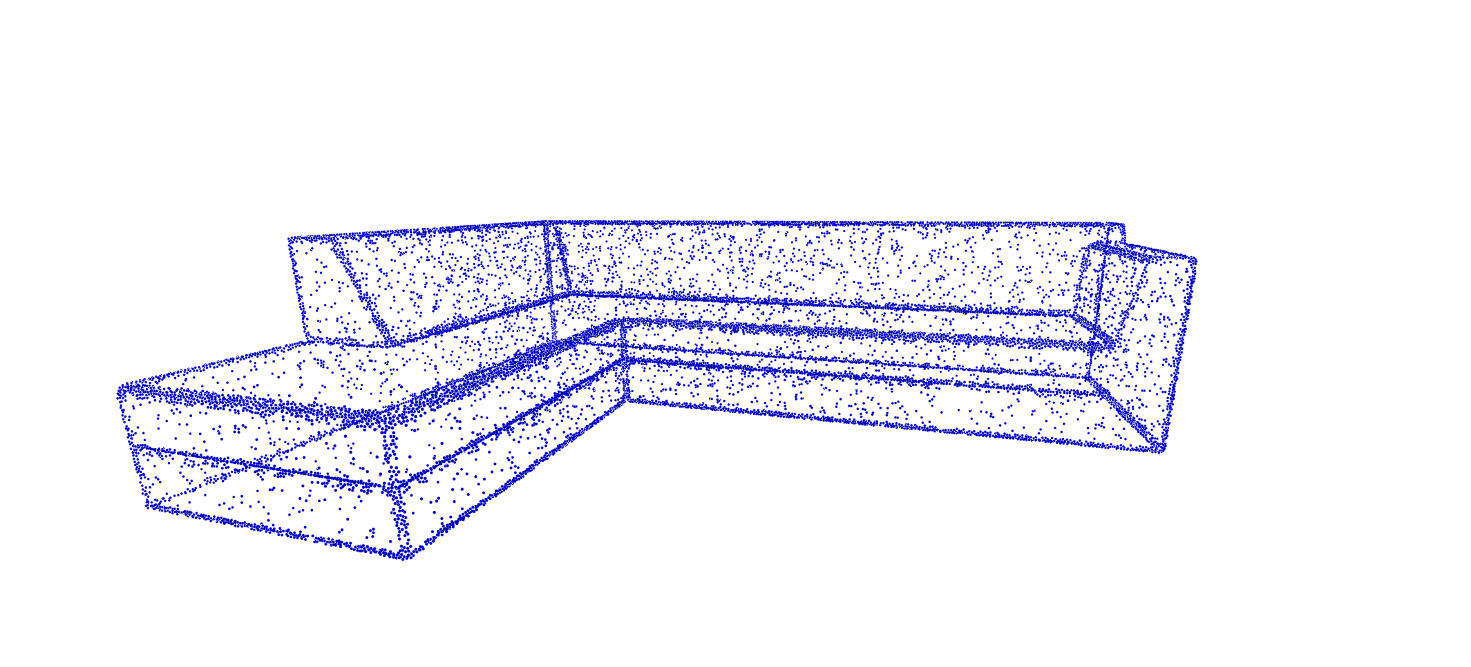
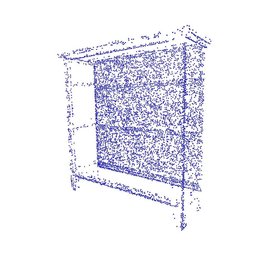
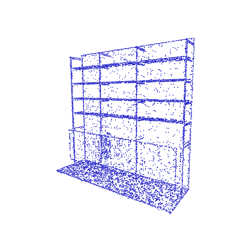
(c) Hypergraph Filtering

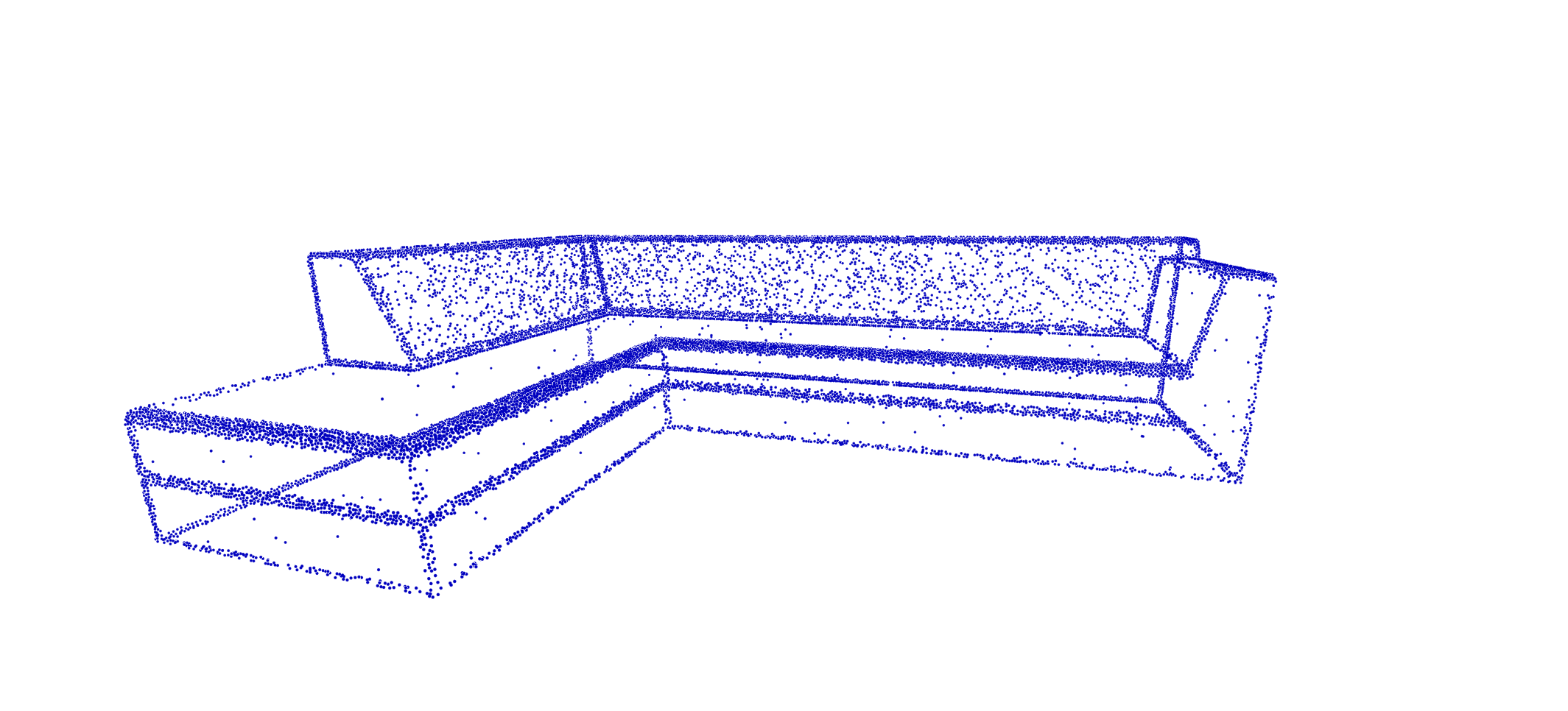
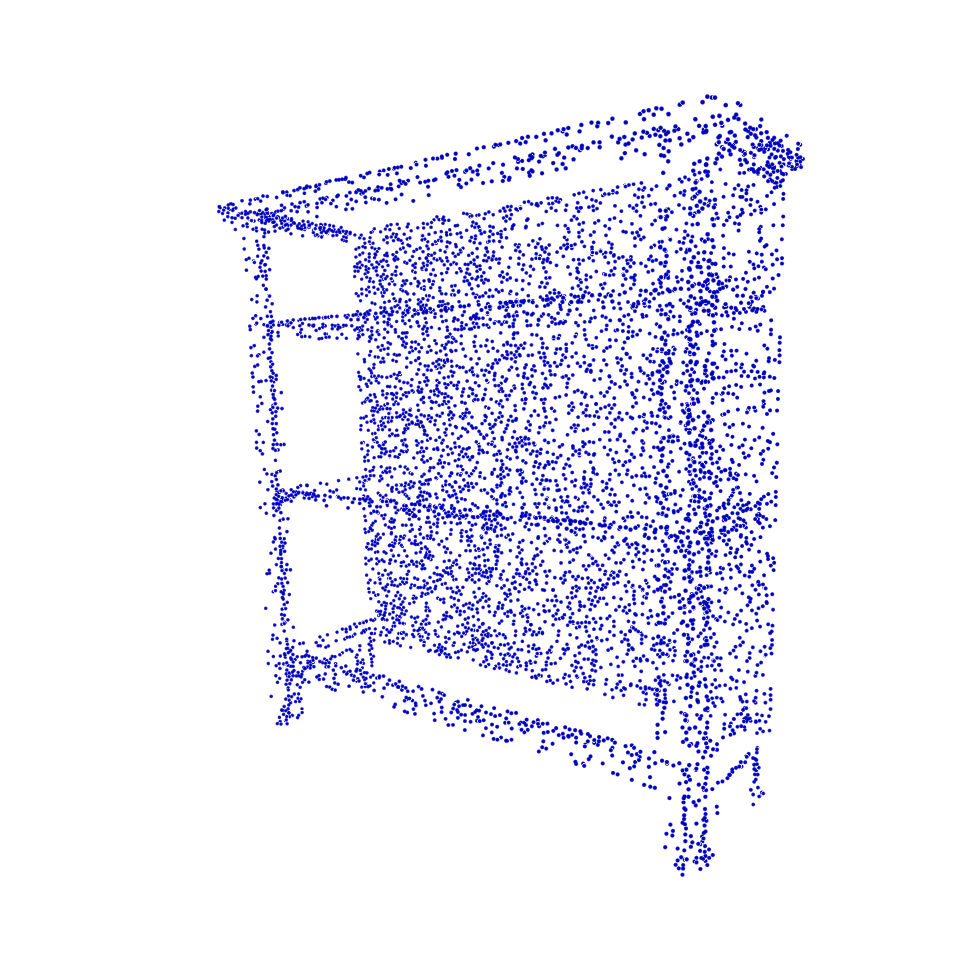
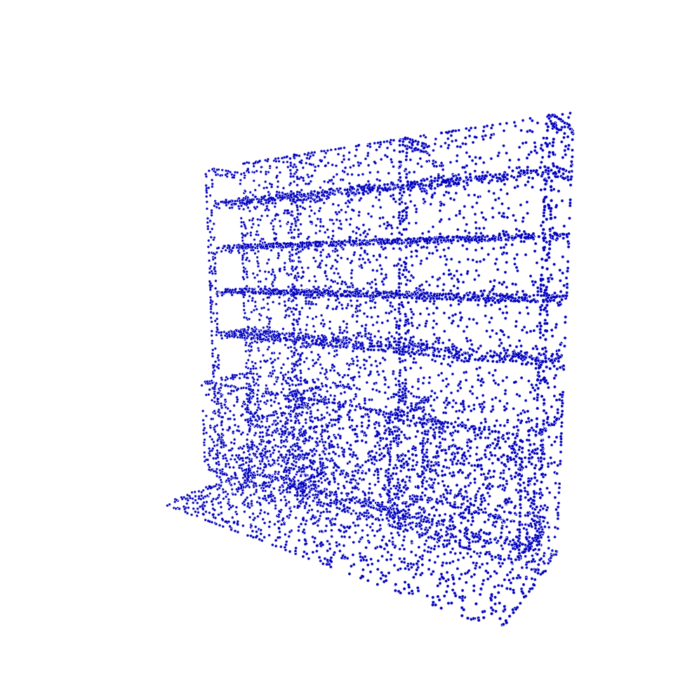
(d) Local Hypergraph Filtering

Figure 6: Examples of Edge Detection for Real Point Cloud.

IV-B Edge Preservation Results on Real-Life Point Clouds

To test our proposed algorithm in a more general setting, we also implement edge-detection based on our resampled data in more complex practical point clouds. For these datasets, there is no explicit ground truth edges to provide quantitative results. Therefore, we present these results as visible point cloud pictures to illustrate the test performance in Fig. 6, where the left column shows original point clouds and the right columns are the three resampled point clouds for our proposed methods, respectively. These results show that our resampling method effectively recover 3D object contours (outlines).

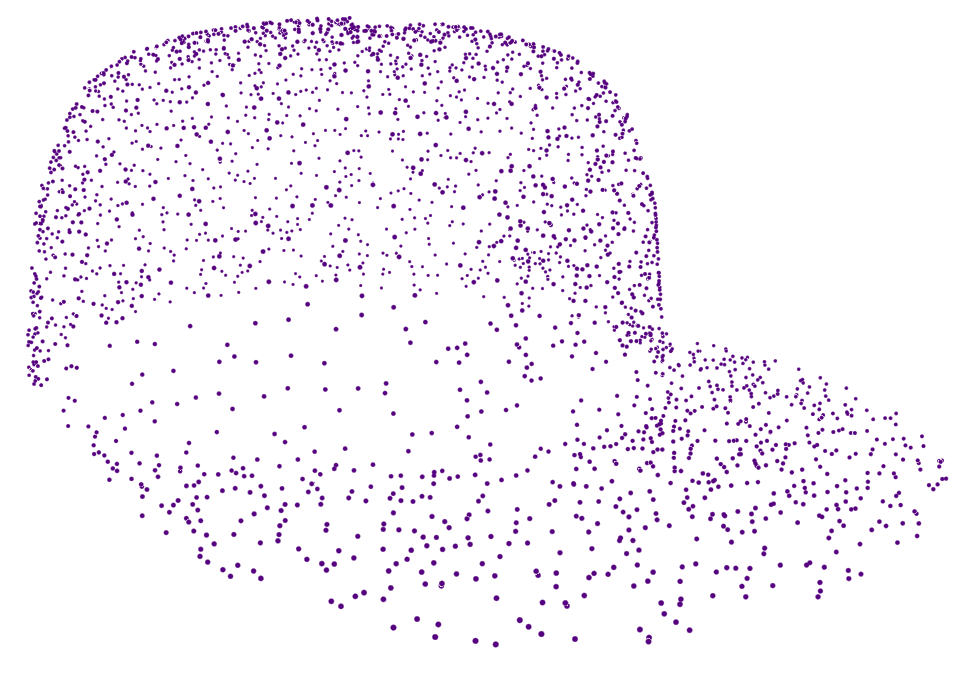
(a) Original Point Cloud of a Cap.

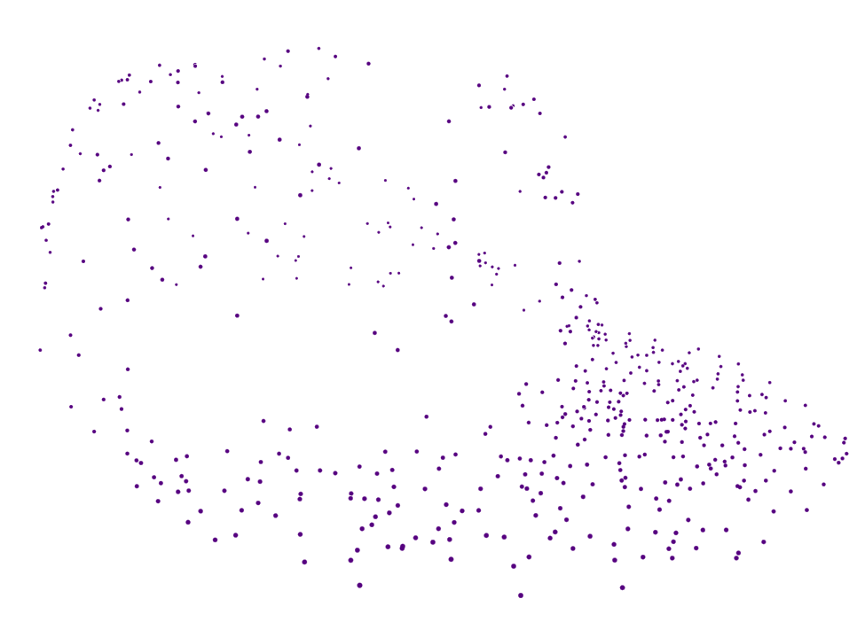
(b) Resampled Result with $\alpha=0.2$.

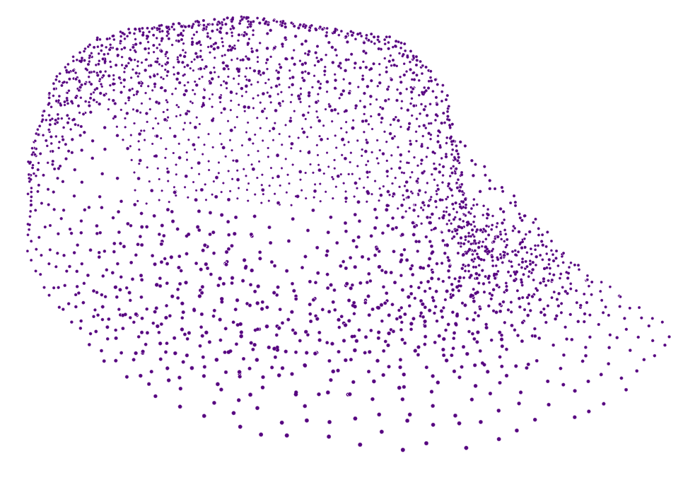
(c) Recovered Point Cloud.

Figure 7: Example of original point cloud, resampled point cloud and the recovered point cloud.

IV-C Point Cloud Recovery from Resampling

In the next test, we investigate the new algorithms’ ability to preserve high degree of point cloud information after resampling. In particular, we shall attempt to recover the dense point cloud after resampling and assess the similarity between the original point cloud and the recovered point cloud from resampling.

Original	HKC	HKF	LHF	GFR	EA	PCA-AC

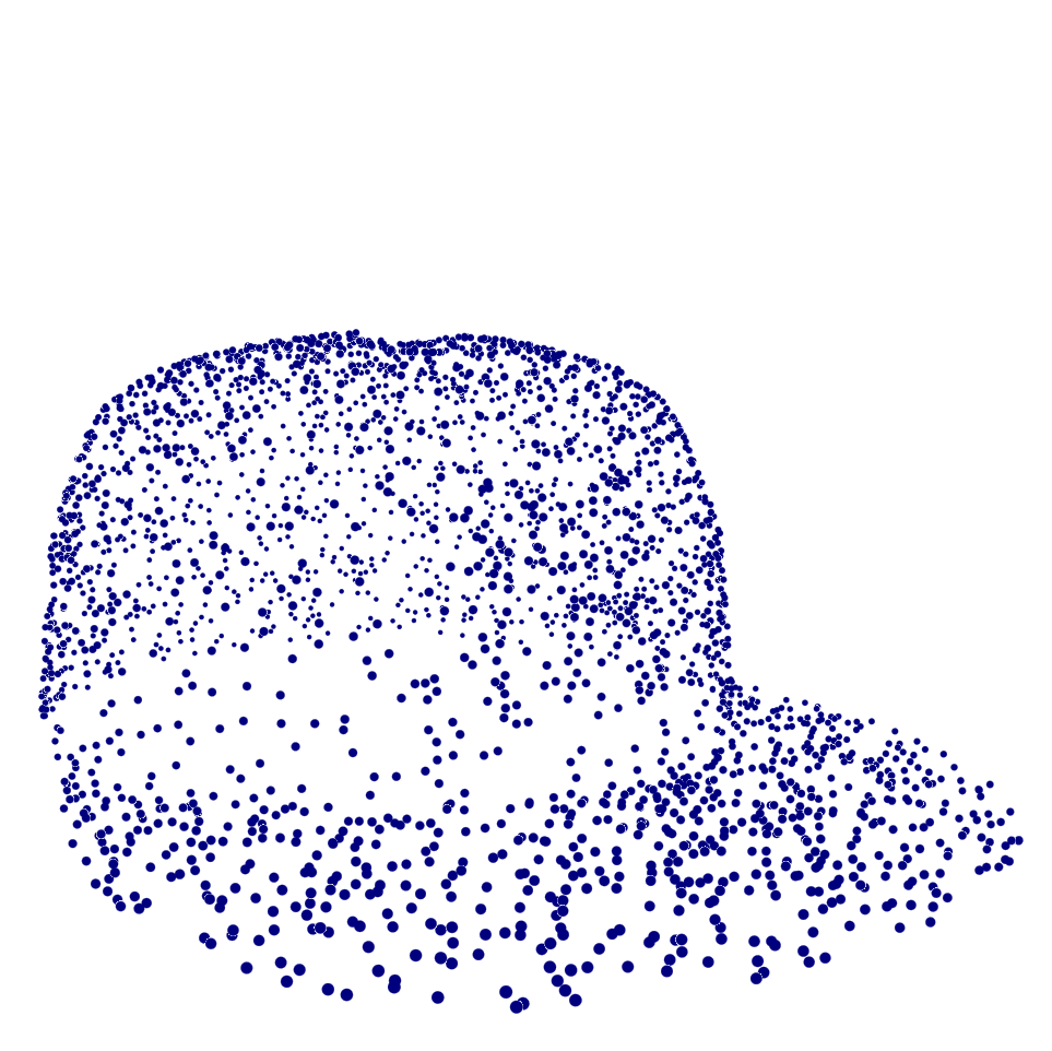
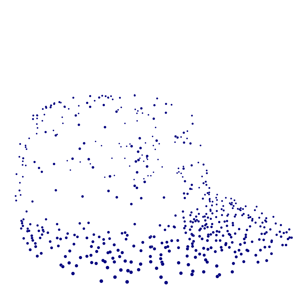
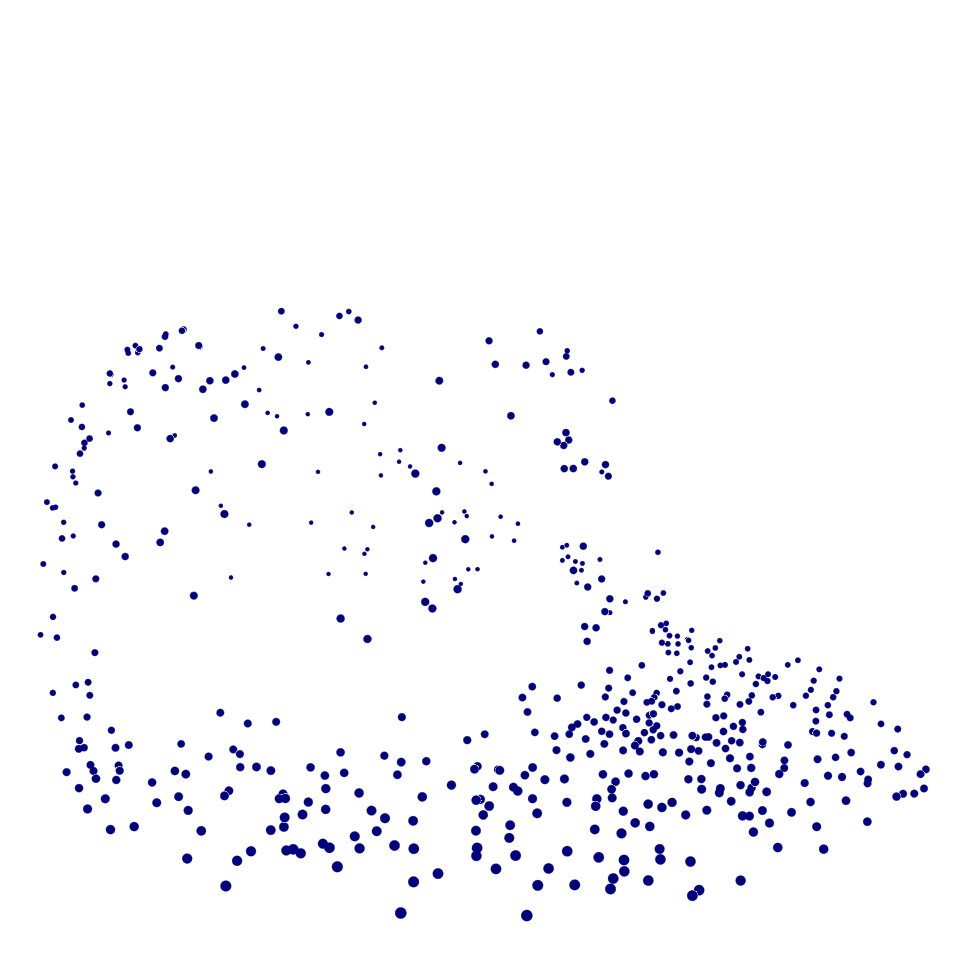
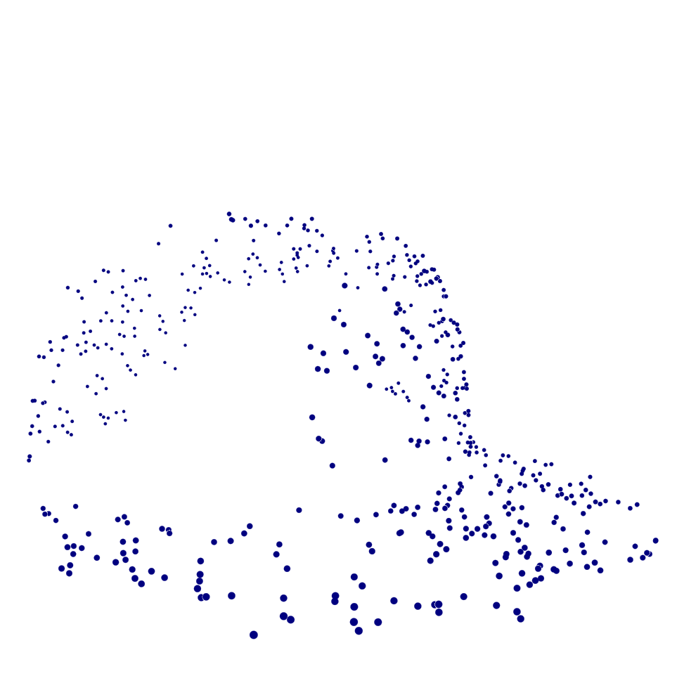
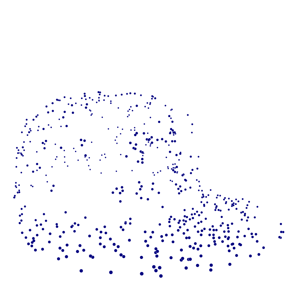
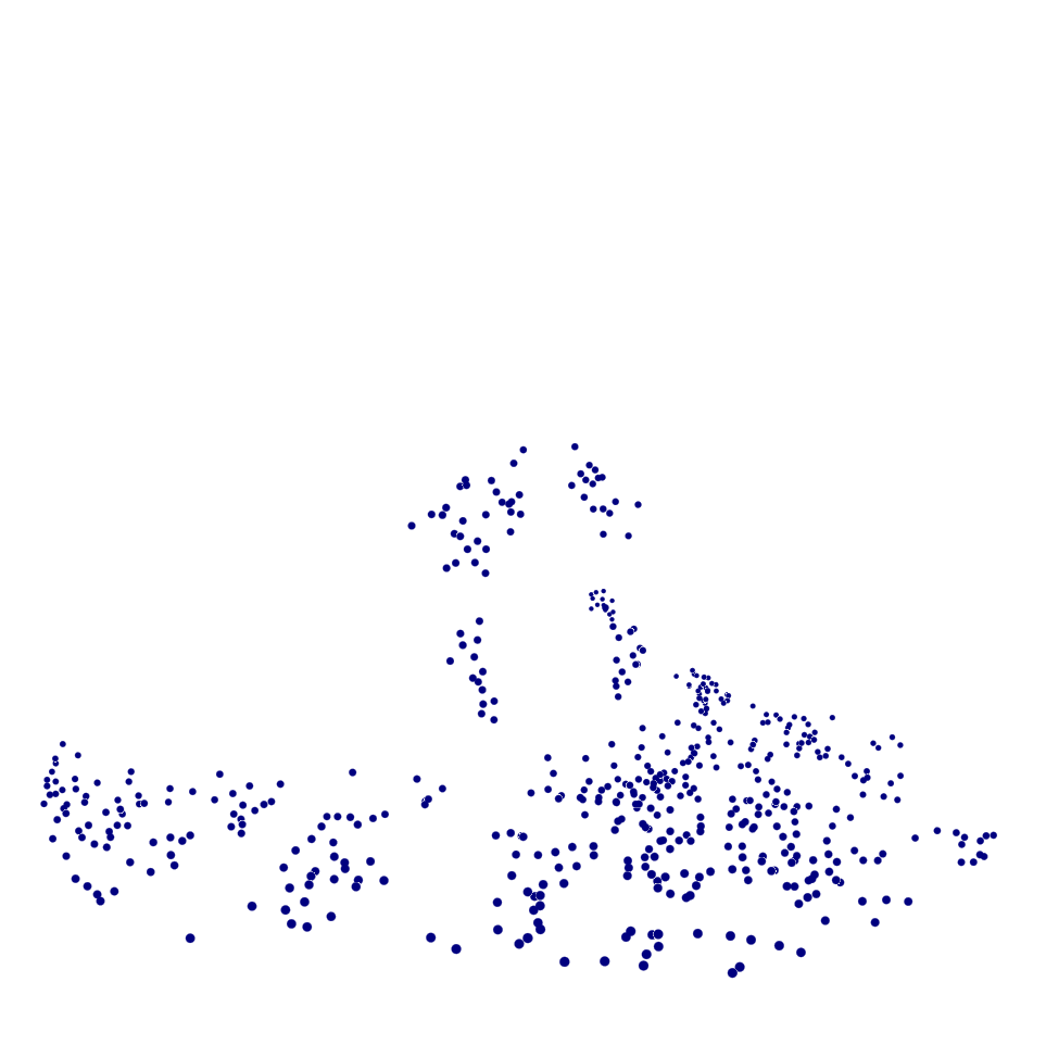
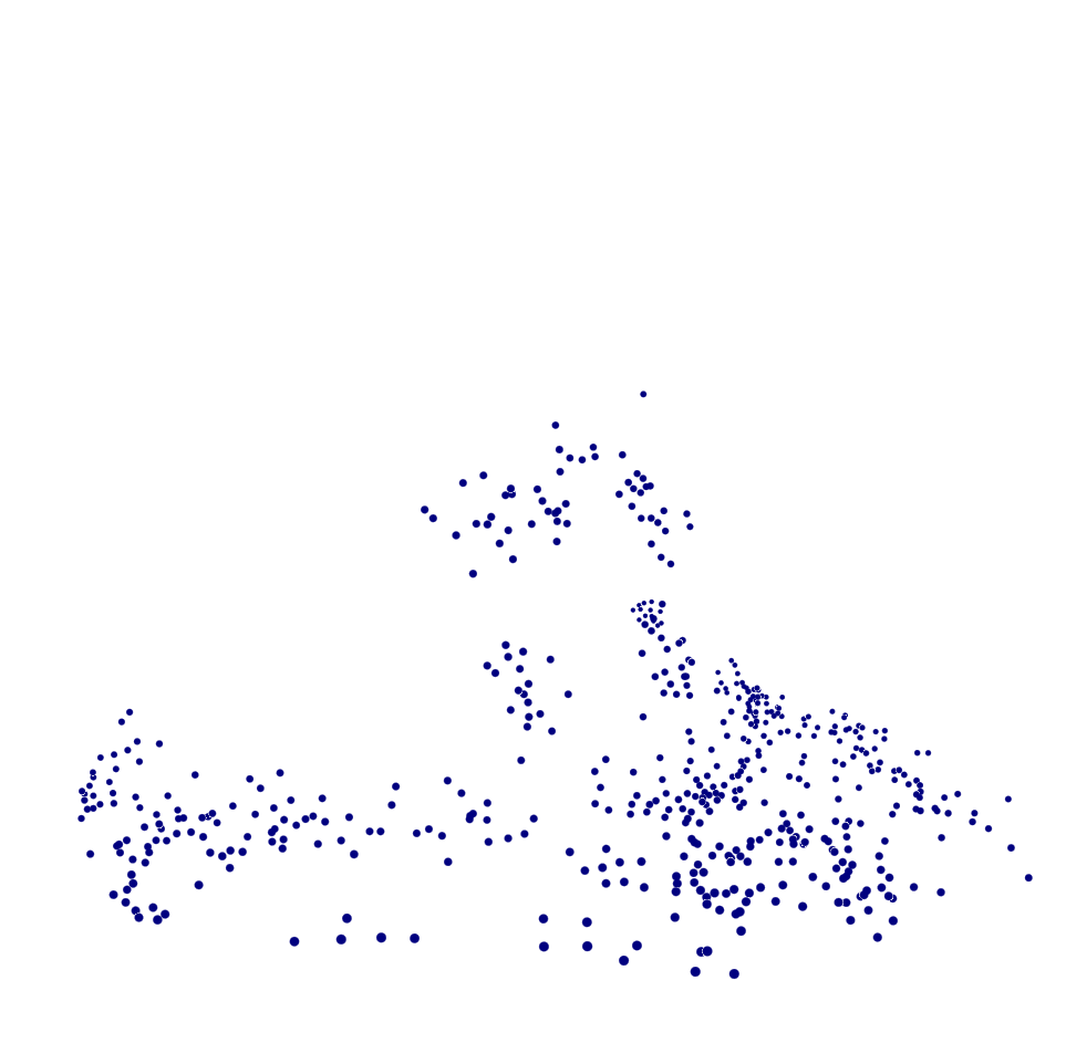
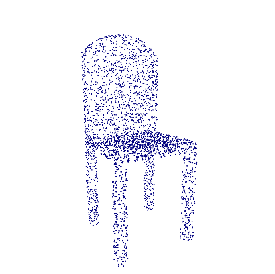
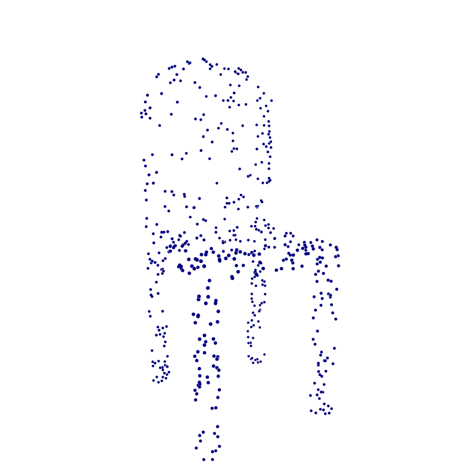
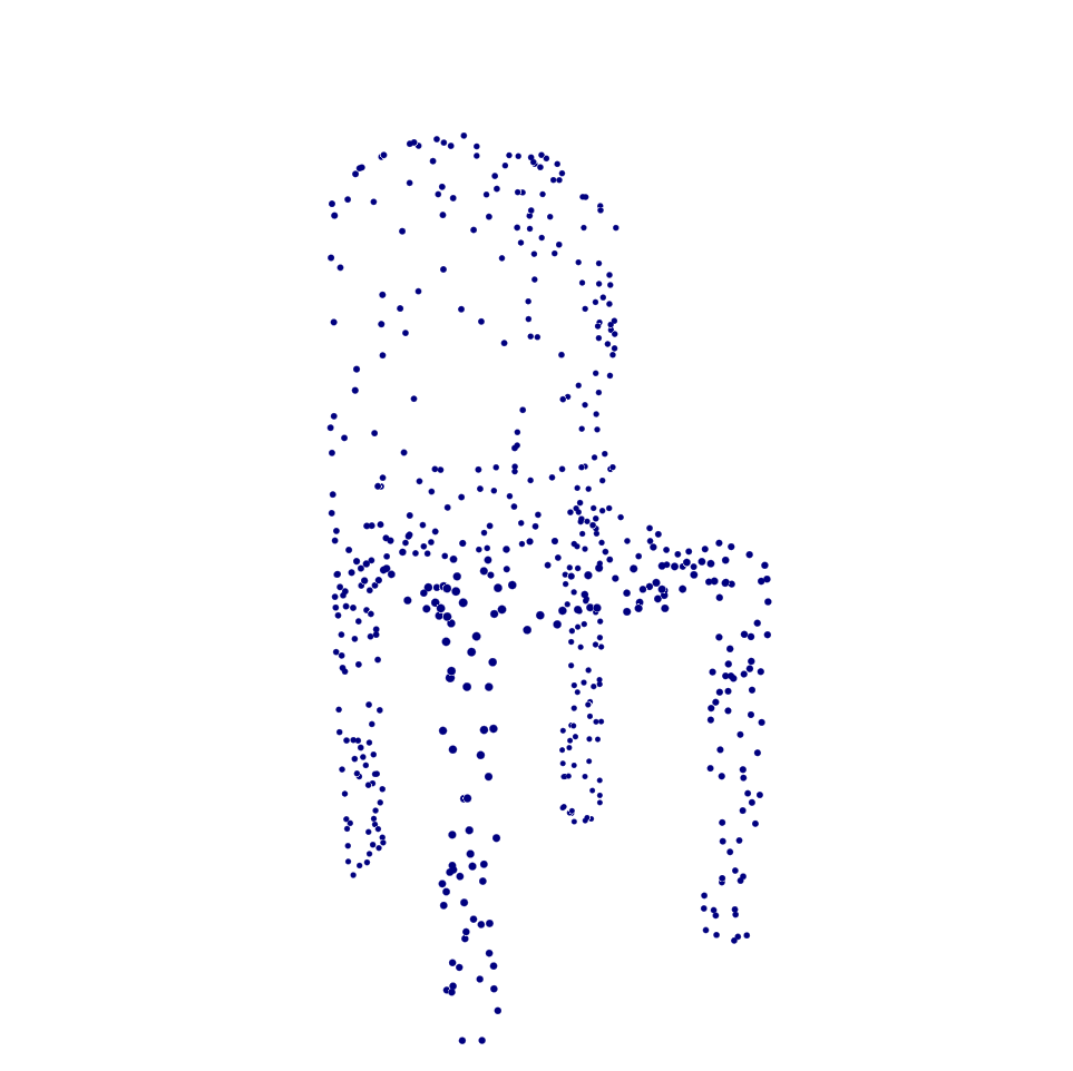
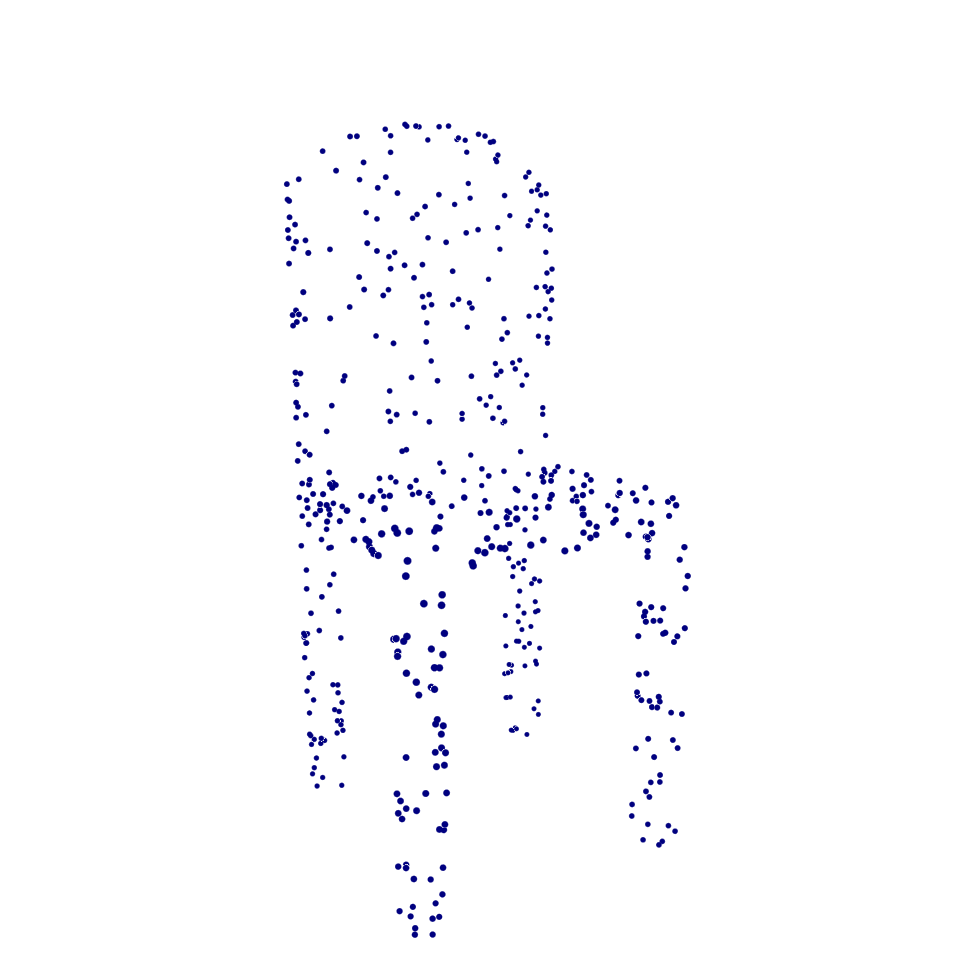
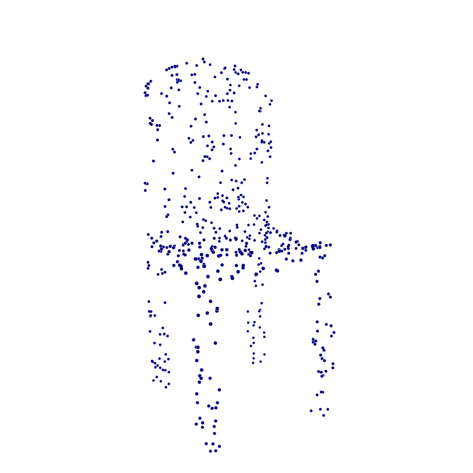
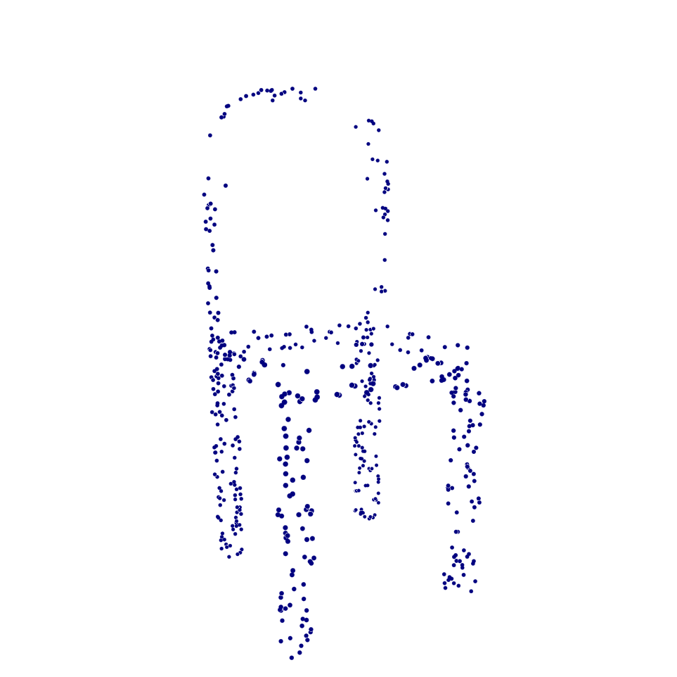
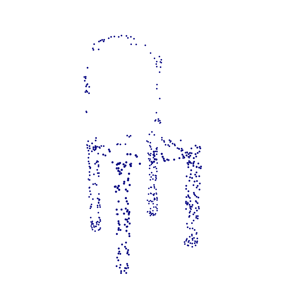
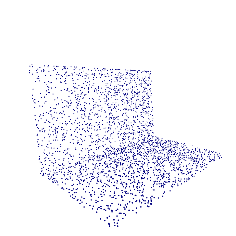
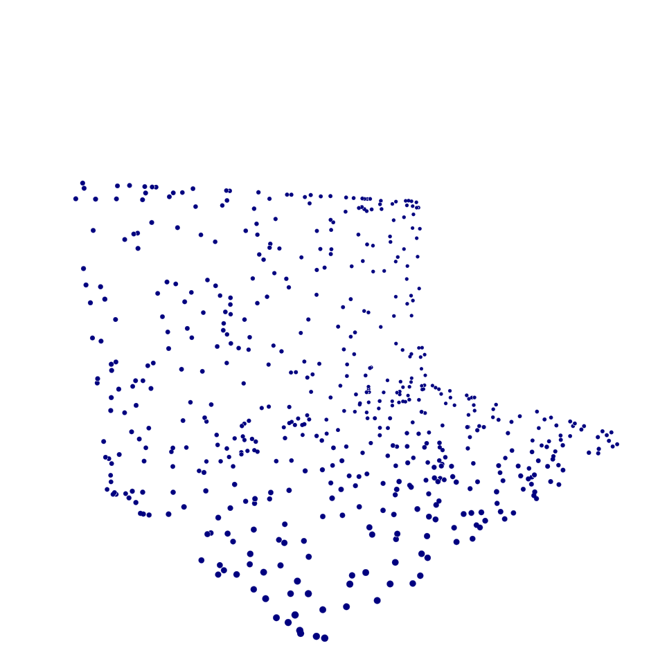
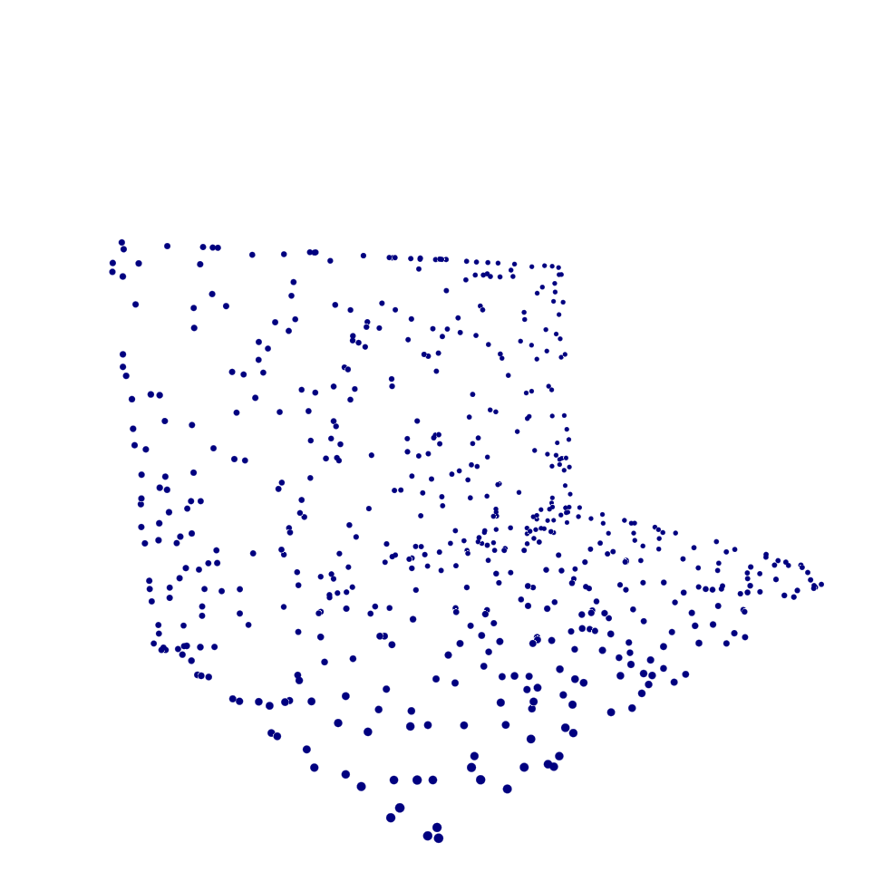
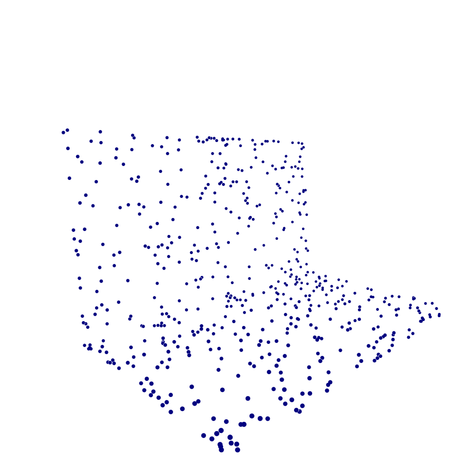
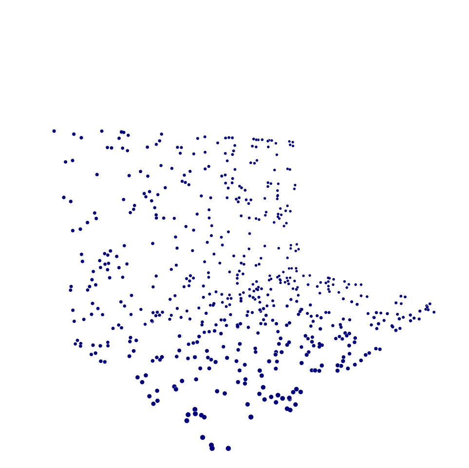
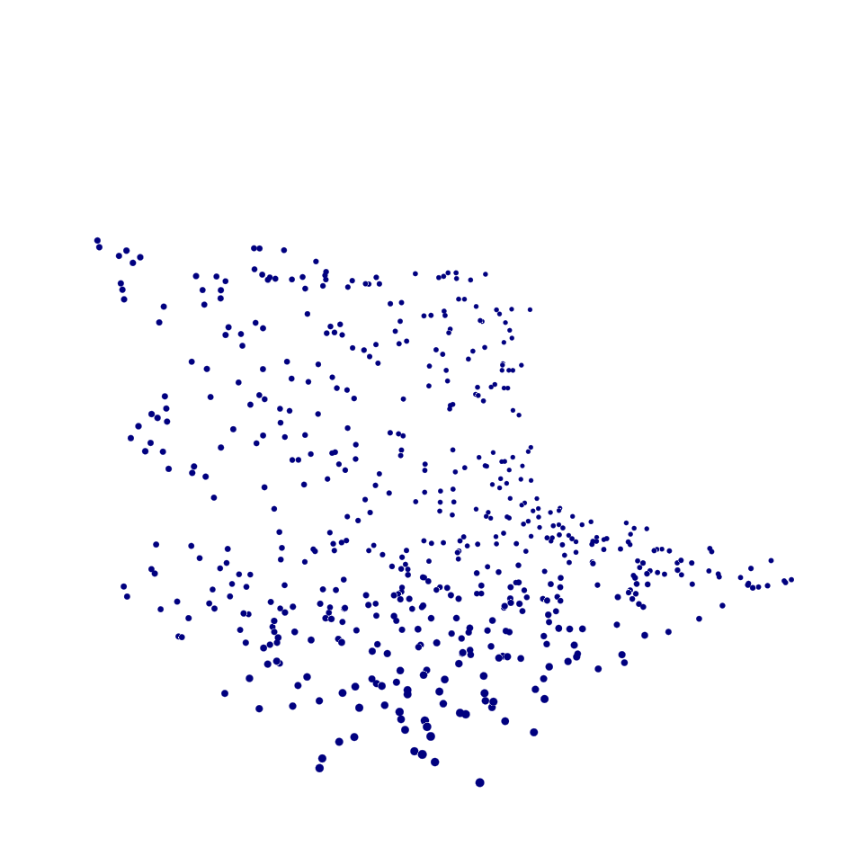
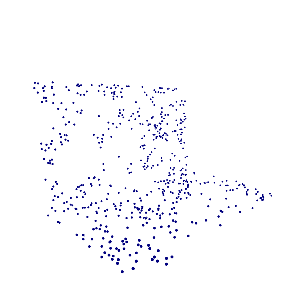
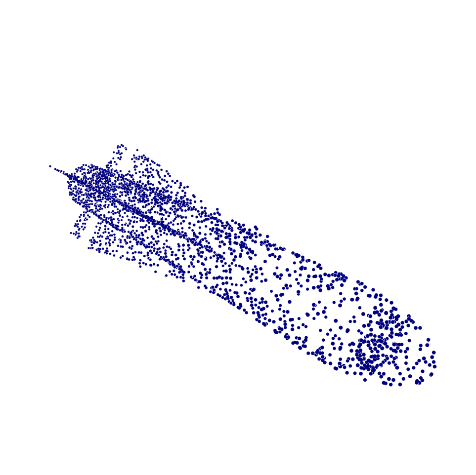
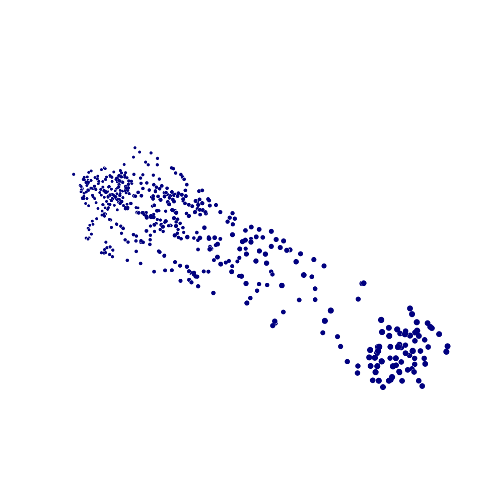
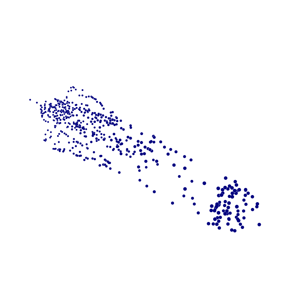
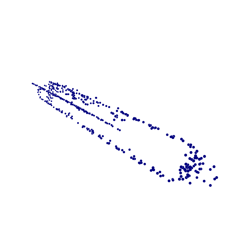
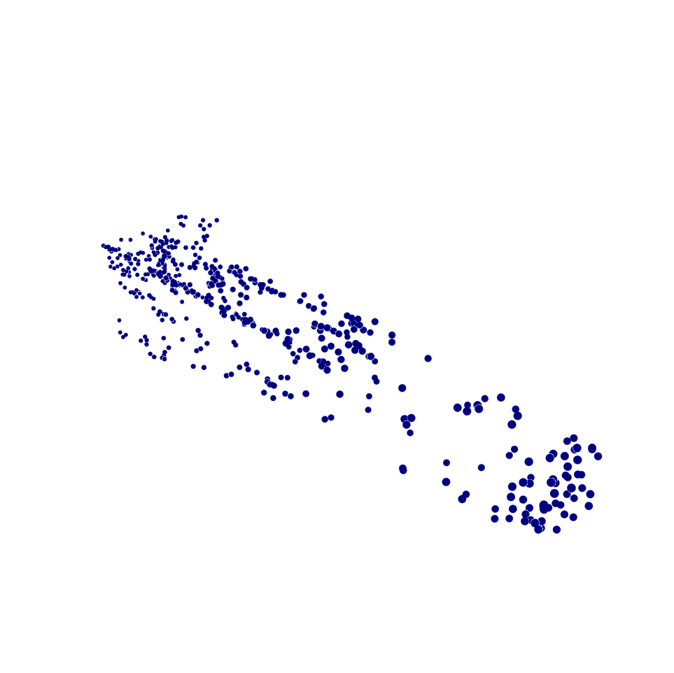
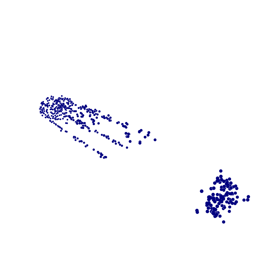
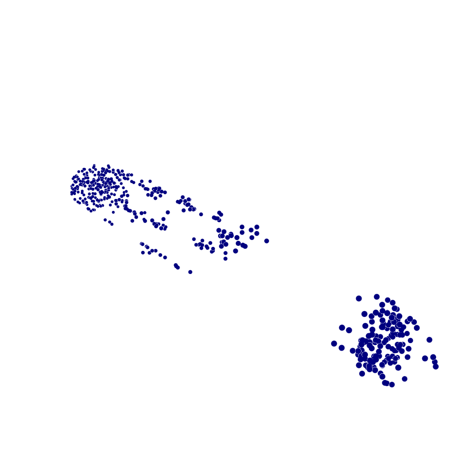
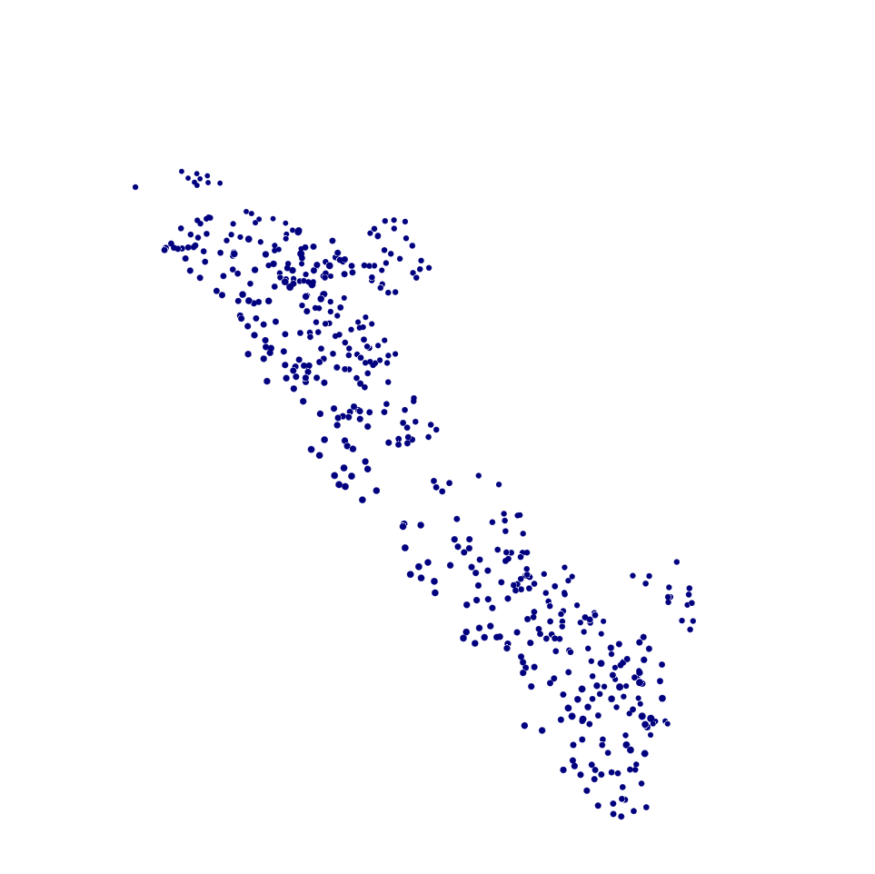
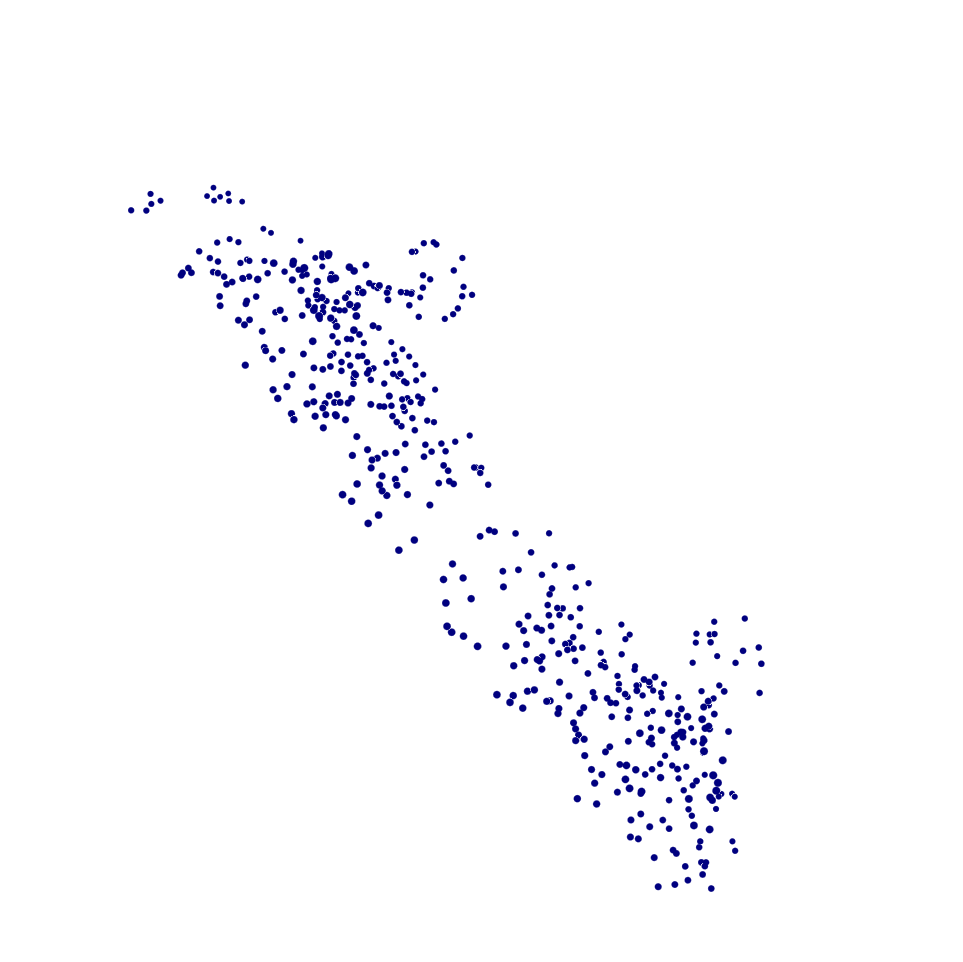
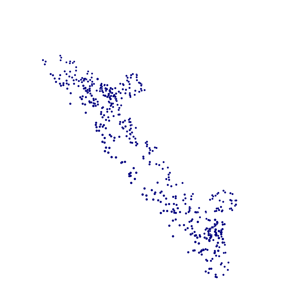
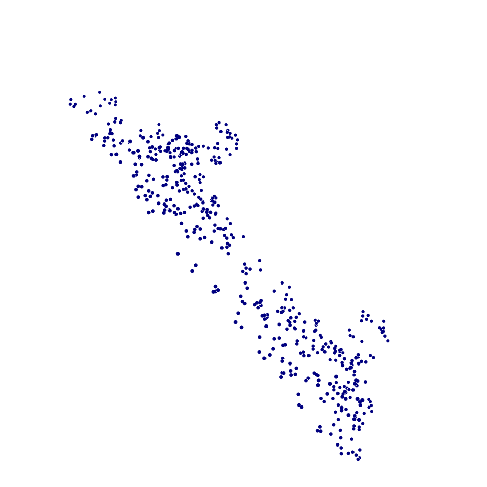
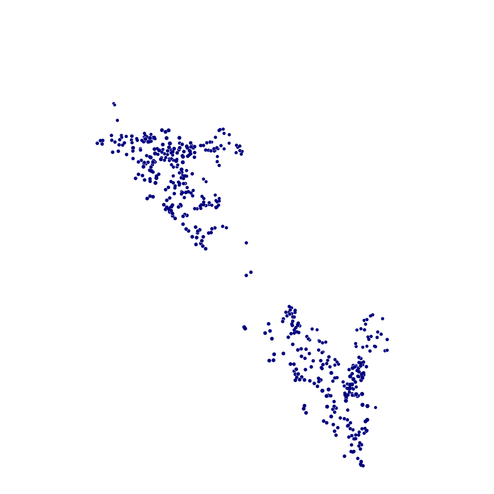
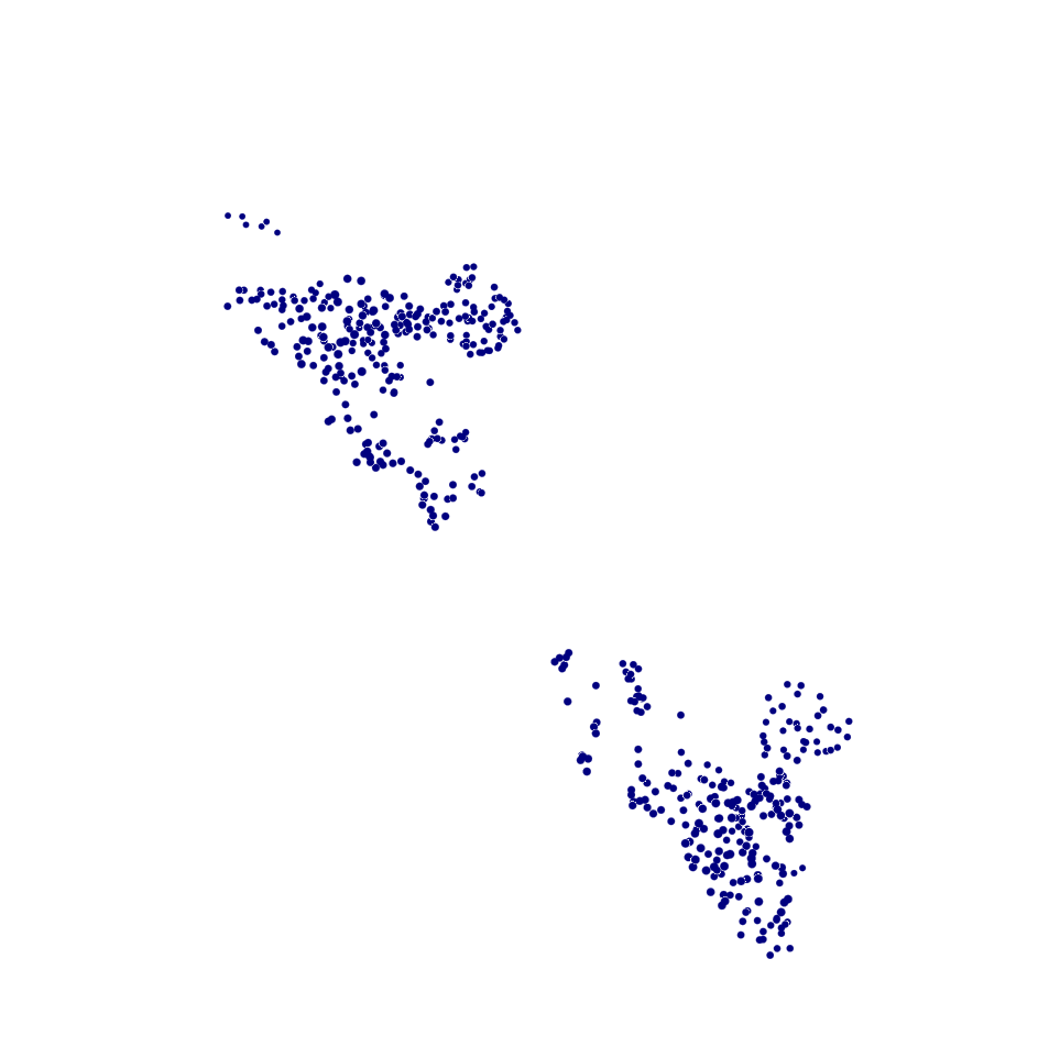
(a) Resampled point clouds

Original	HKC	HKF	LHF	GFR	EA	PCA-AC

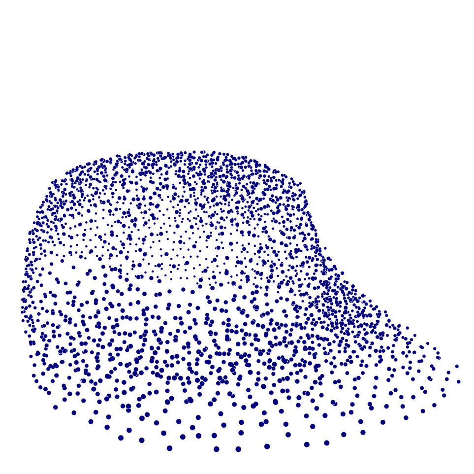
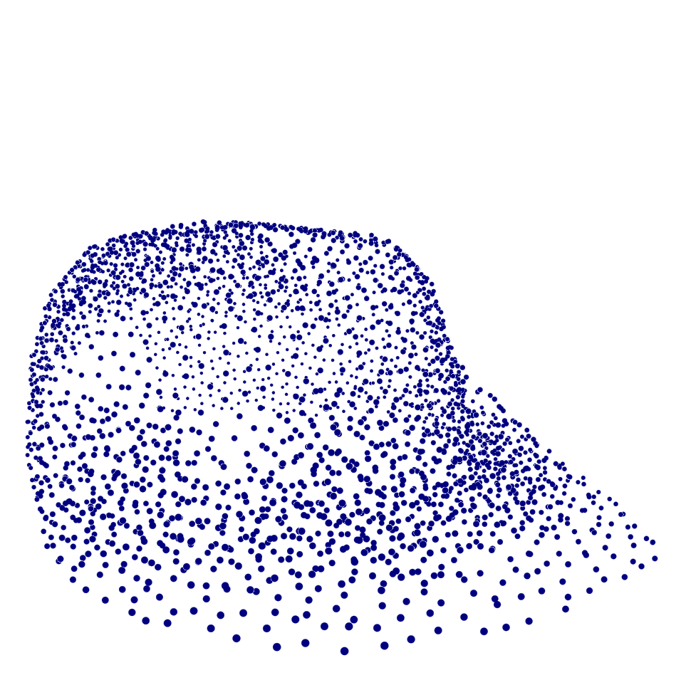
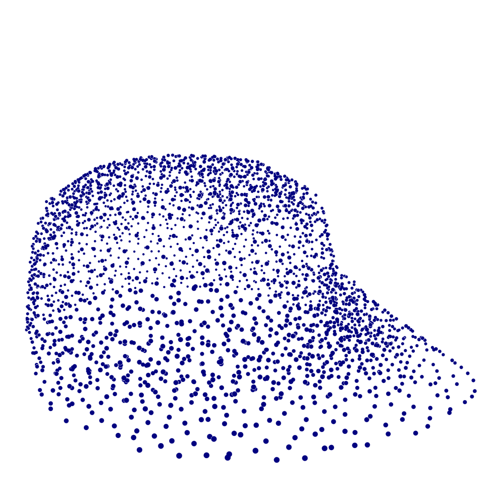
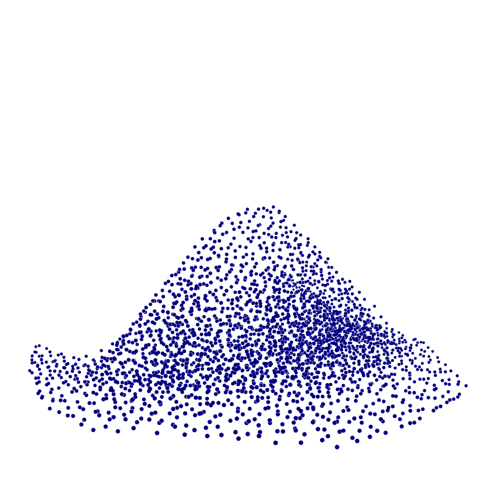
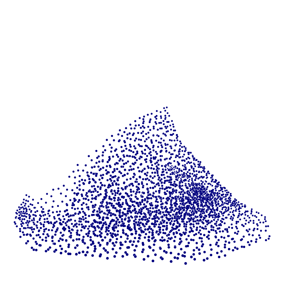
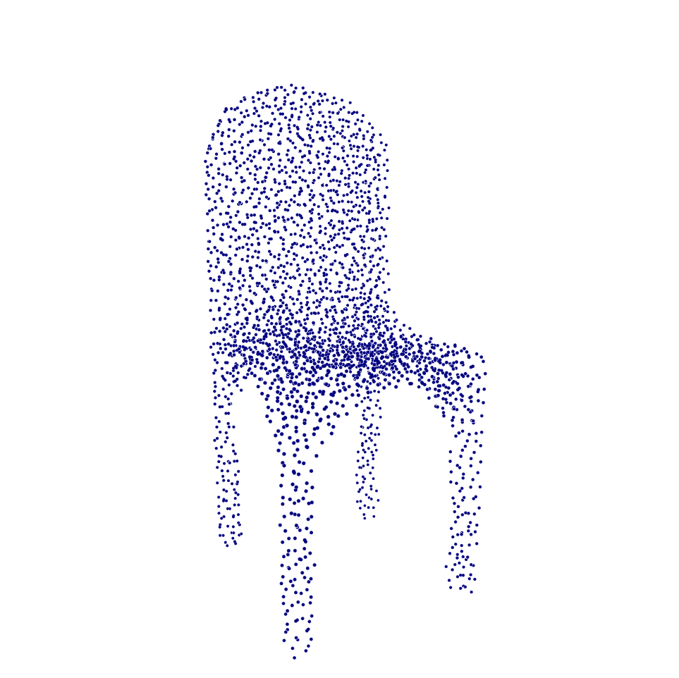
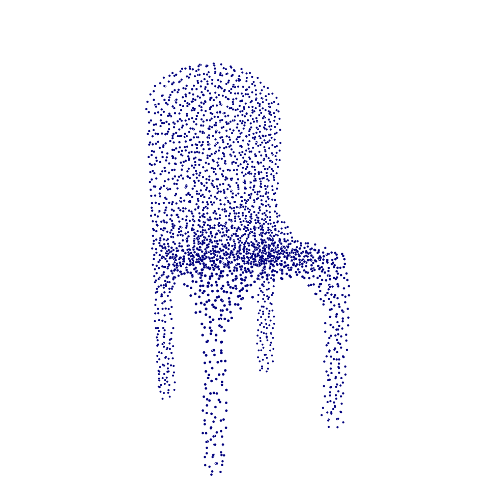
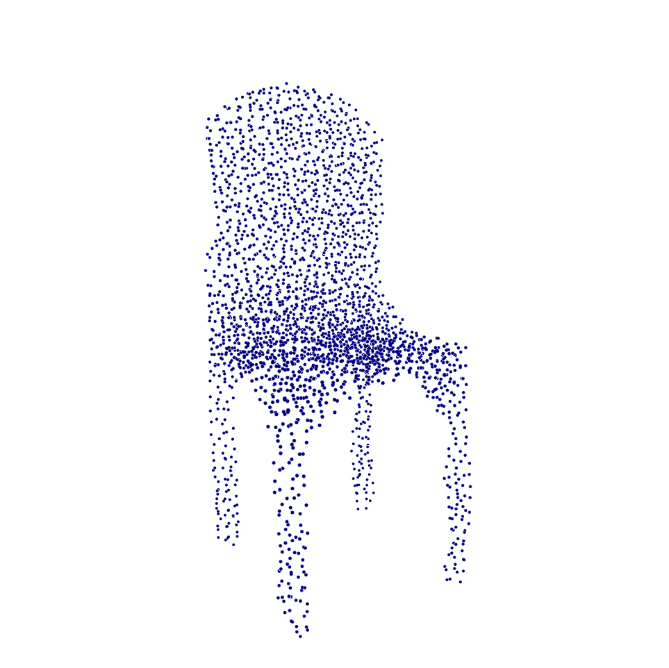
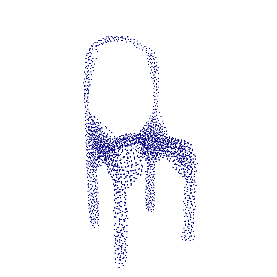
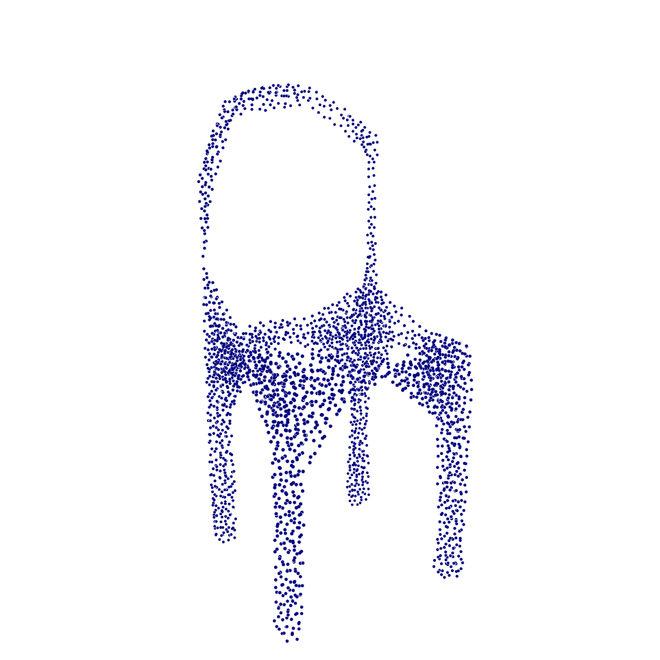
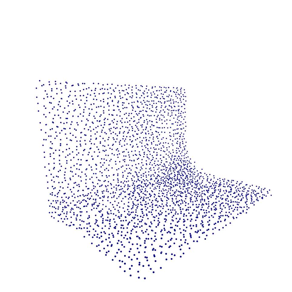
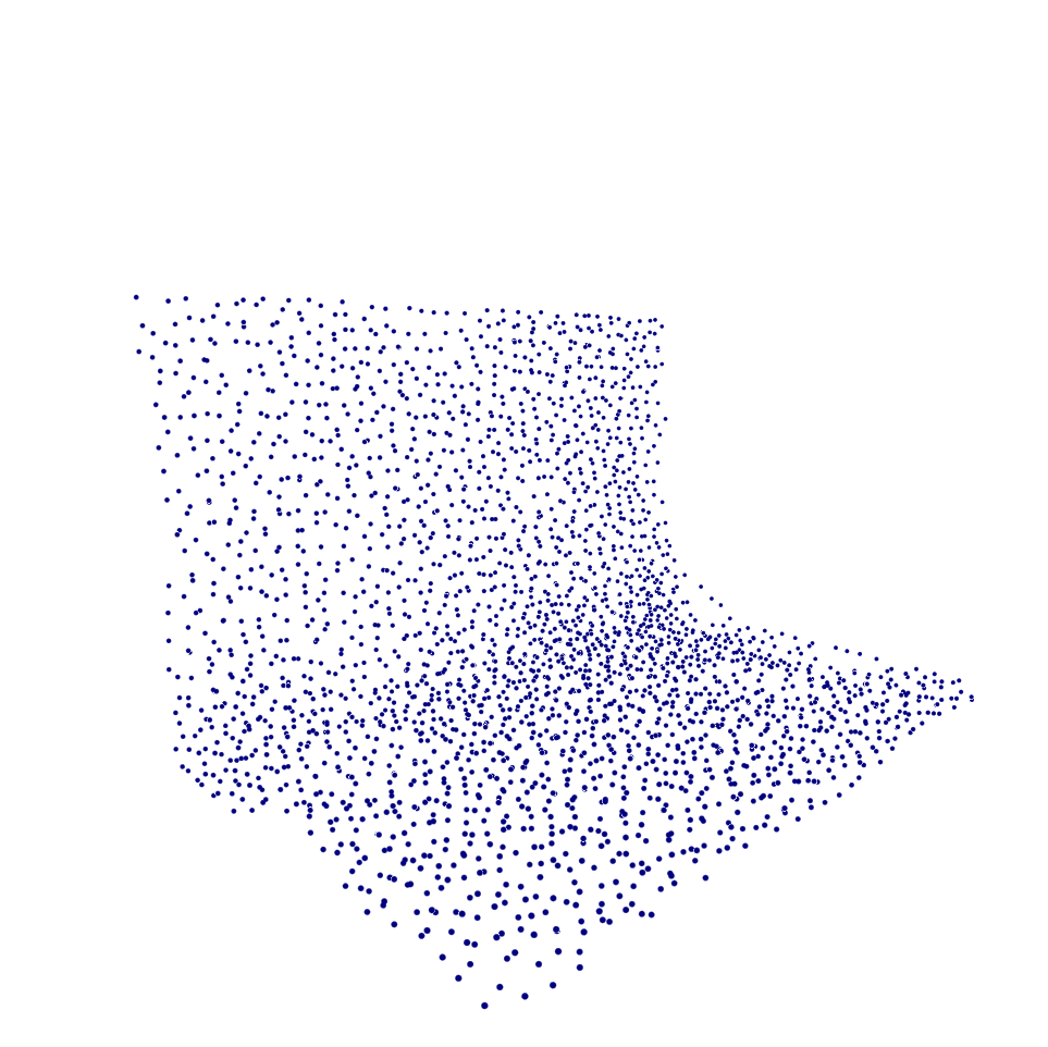
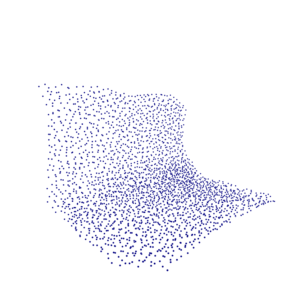
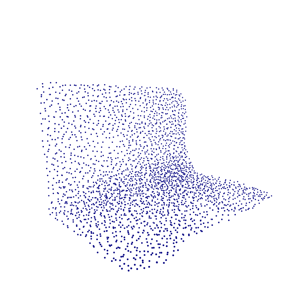
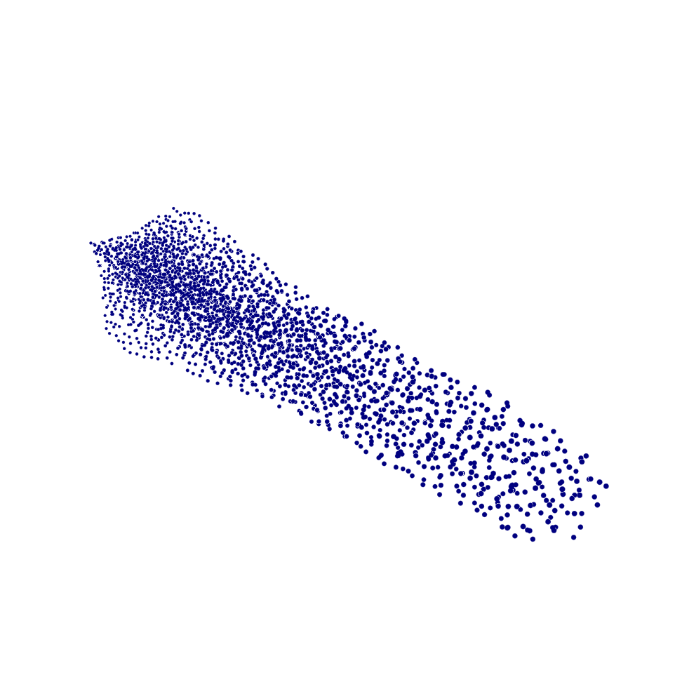
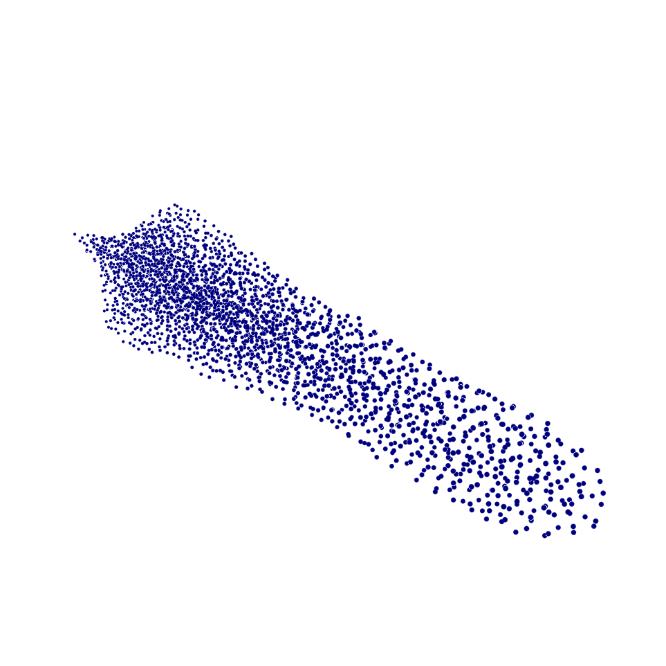
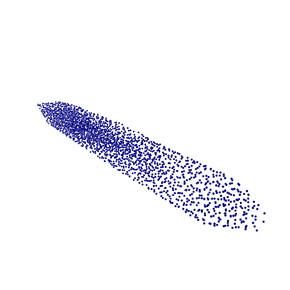
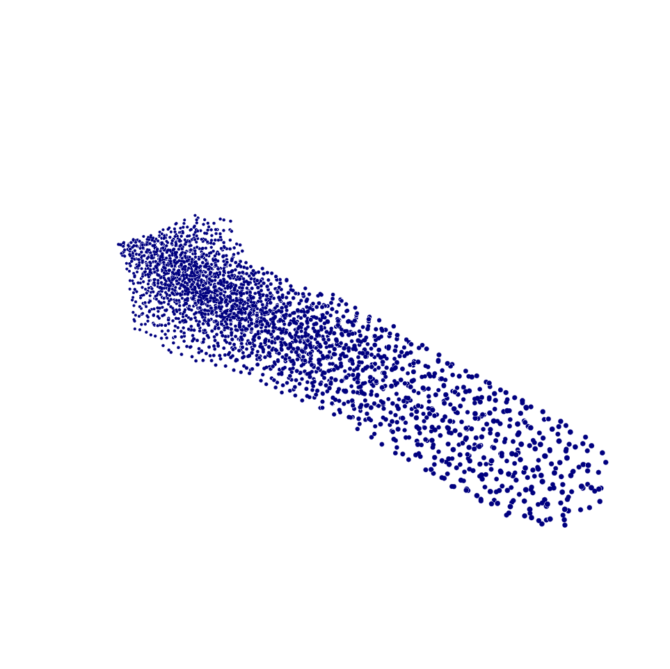
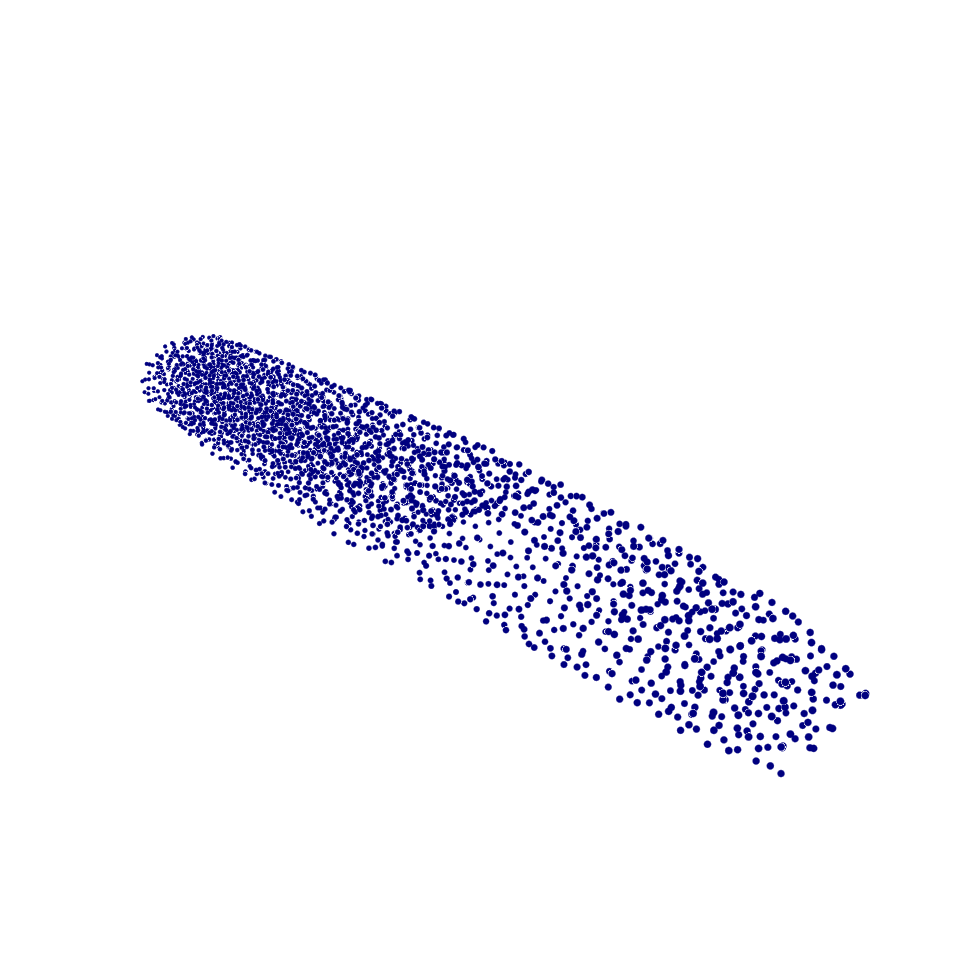
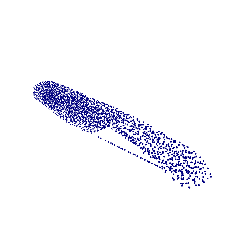
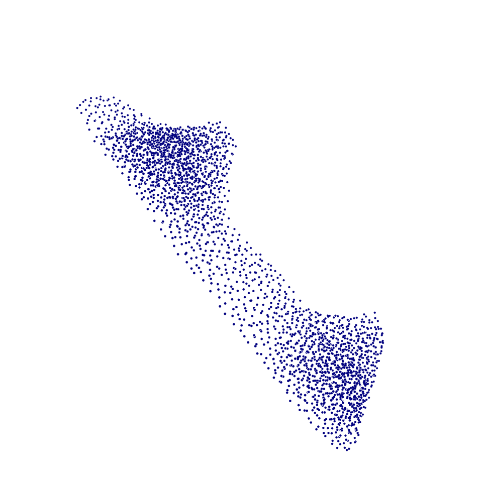
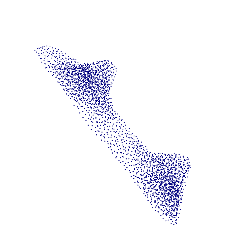
(b) Recovered point clouds.

Figure 8: Example of original, resampled and recovered point clouds with resampling ratio $\alpha=0.2$.

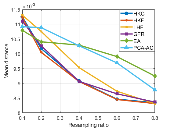
(a) Mean distance against $\alpha$.

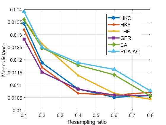
(b) Average of distance and dual distance against $\alpha$.

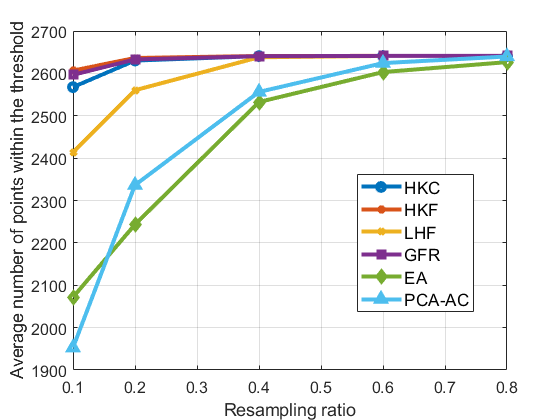
(c) Average number of points in recovered point cloud $d_{\theta}$ against $\alpha$.

Figure 9: Plots of recovered accuracy against resampling ratio $\alpha$ of all methods

IV-C1 Dense Point Cloud Recovery

A typical method for dense point cloud recovery consists two steps: a) reconstructing the surface of object from the resampled point cloud; and b) sampling the reconstructed object surface to generate a recovered point cloud. Since points of edge preserving resampled point clouds tend to concentrate near areas of high local variations, e.g., edges/corners, points of these resampled point clouds are not uniformly distributed, as shown in Fig. 7(b). For this reason, some generic surface reconstruction methods such as Poisson reconstruction [29] may perform poorly on such sparse point clouds. We must pay special attention to surface reconstruction methods chosen for such type of resampled point cloud data.

In order to reconstruct surfaces from edge preserving and sparsely resampled point clouds, we propose to first construct the alpha complex [30] from the resampled point cloud. To mitigate the potentially degrading impact of imperfect reconstruction, we decide to reconstruct six different surface models for each resampled point cloud by applying different parameters. We then apply Poisson-disk resampling to sample the alpha complex to form a recovered point cloud. To further mitigate the effect due to the possible construction of extraneous surfaces absent from the original object, we select a threshold distance $d_{\theta}$ three times the intrinsic resolution of the original point cloud. Using the threshold distance, we only retain the best recovered point cloud which contains the largest number of points that are within the threshold distance $d_{\theta}$ from the original point cloud.

IV-C2 Distance Between Point Clouds

To assess the quality of point cloud recovery, we need to define distances between the original and the recovered point clouds. Let $p_{i}$ denote a point in the original and $p_{c,j}$ denote a point in the recovered point cloud. When computing our distance between two point clouds, we neglect any distances between point $p_{i}$ in the original point cloud and $p_{c,j}$ in the recovered point cloud such that the minimum distances $\min_{j}\|p_{i}-p_{c,j}\|$ and $\min_{i}\|p_{i}-p_{c,j}\|$ are greater than $d_{\theta}$.

We define a distance and a dual distance between the original and the recovered point cloud as

$$D_{0}=\frac{1}{N_{1}}\sum_{i=1}^{N_{1}}\min_{j:\|p_{i}-p_{c,j}\|<d_{\theta}}\|p_{i}-p_{c,j}\|,$$ (18)

$${\check{D}}_{0}=\frac{1}{N_{2}}\sum_{j=1}^{N_{2}}\min_{i:\|p_{i}-p_{c,j}\|<d_{\theta}}\|p_{i}-p_{c,j}\|,$$ (19)

where $N_{1}$ is the number of points in the original point cloud that satisfy $\|p_{i}-p_{c,j}\|<d_{\theta}$ for some $p_{c,j}$ and $N_{2}$ is the number of points in the recovered point cloud that satisfy $\|p_{i}-p_{c,j}\|<d_{\theta}$ for some $p_{i}$. In other words, $D_{0}$ is the average distance for points that are in the original point cloud within $d_{\theta}$ from the closest points in the best recovered point cloud. The dual distance ${\check{D}}_{0}$ is the average distance for points in the best recovered point cloud that are within $d_{\theta}$ from their closest points in the original point cloud.

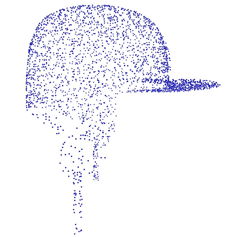
(a) Original Point Cloud.

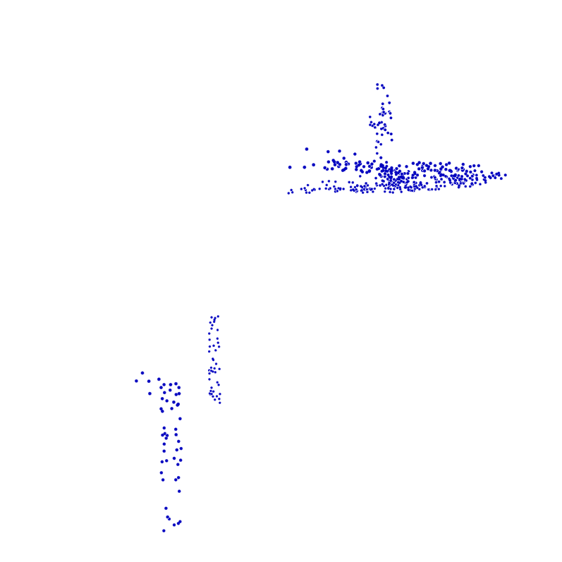
(b) Resampled Point Cloud.

Figure 10: Example of results from the EA method for $\alpha=0.2$.

IV-C3 Visual and Numerical Results

We use six different categories of point clouds from ShapeNet [31] in our experiments. Similar to experiments discussed earlier, we test our HKF method together with the GSP-based GFR method in [7] plus the EA and PCA-AC methods from [14]. For fairness, we use the same resampling ratio for all the methods.

Our experiments follow the following steps. First, we apply resampling and edge detection methods to calculate the resampled point clouds with resampling ratio $\alpha$. Next, we apply our proposed recovery method to generate recovered point clouds. Based on the resampled point clouds, we compute the numerical performance metrics for different algorithms in comparison. We measure the performance under three metrics: 1) distance defined in Eq. (18); 2) average of distance and dual distance as defined in Eq. (18) and Eq. (19), respectively; and 3) average number $N_{1}$ of points within the threshold $d_{\theta}$ between the original and recovered point cloud. Smaller distance and larger number of points within the threshold indicate better performance.

To start, Fig. 8 provides a set of the resampled point clouds and their corresponding recovered ones from different methods. Visual inspection shows that our proposed HKC, HKF, and LHF algorithms generally deliver consistently strong results in resampling and recovery of point clouds, regardless of the dataset under study.

Categories	HKC	HKF	LHF	GFR	EA	PCA-AC
Cap	0.0111	0.0101	0.0117	0.0102	0.0087	0.0115
Chair	0.0111	0.0113	0.0116	0.0118	0.0125	0.0126
Laptop	0.0106	0.0106	0.0103	0.0105	0.0110	0.0110
Mug	0.0134	0.0134	0.0150	0.0141	0.0150	0.0147
Rocket	0.0069	0.0069	0.0078	0.0070	0.0070	0.0073
Skateboard	0.0079	0.0080	0.0080	0.0079	0.0082	0.0083

(a) Mean distance between the best recovered point cloud and the corresponding original point cloud.

Categories	HKC	HKF	LHF	GFR	EA	PCA-AC
Cap	2628.3	2632.4	2315.7	2635	1427.5	2160.4
Chair	2656.1	2657.9	2658	2653.9	2458.2	2469.9
Laptop	2754.4	2784.4	2785.6	2774.3	2626.4	2584.6
Mug	2818.6	2819.9	2716.6	2810.7	2633.7	2418.2
Rocket	2364.4	2361	2317.4	2360.6	1904.4	2004.5
Skateboard	2559.8	2562	2568.2	2563.1	2409.9	2381.2

(b) Average number of points within $d_{\theta}$ between the best recovered point cloud and the corresponding original point cloud.

TABLE III: Mean distance and the average number of points within $d_{\theta}$ between the best recovered point cloud and the original point cloud for resampling ratio $\alpha=0.2$.

To quantitatively illustrate the performance comparison, Table. III presents the numerical results for $\alpha=0.2$. From the test results, we observe that our HKF algorithm exhibits the best performance in terms of both mean distance and number of matched points versus the traditional GFR graph method and two edge detection methods. Compared with the edge detection methods, our proposed algorithms consistently retain larger numbers of points within the threshold $d_{\theta}$ in most point cloud categories.

The comparison also demonstrates a potential issue of the specialized edge detection based methods. In particular, resampled point cloud of edge detection methods may over-emphasize only part of the original point cloud, as the example of “cap” in Fig. 10 shows. As a result, substantial number of points may not be retained by the generic edge detection methods during resampling.

We also examine the effect of sampling ratio $\alpha$ and graphically illustrate the variation of mean distance, average of distance and dual distance, and average number within threshold against different sampling ratios in Fig. 9. Here we use the same set of point clouds in the numerical results for $\alpha=0.2$. It is clear and intuitive that higher resampling ratio leads to better performance of all methods under study. It is important to note that our proposed methods exhibit performances superior to the traditional methods in terms of mean distance for various resampling ratios. This result indicates that our proposed hypergraph-based methods tend to preserve the geometric information more efficiently in resampling. The hypergraph-based methods also exhibits better results with respect to the number of corresponding nodes between reconstructed and original point clouds.

In summary, our test results demonstrate the efficiency of the proposed resampling while preserving the underlying structural features and geometric information among point cloud data. They further demonstrate that hypergraph presents a promising alternative beyond regular graph for modeling point clouds in some point cloud related applications.

V Conclusion

This work investigates new ways for efficient and feature preserving resampling of 3D point cloud based on hypergraph signal processing (HGSP). We establish HGSP as an efficient tool to model multilateral point relationship and to extract features in point cloud applications. We propose three new methods based on HGSP kernel convolution and spectrum filtering. Although typical HGSP tools tend to require high computational complexity, our proposed algorithms bypass certain steps for hypergraph construction and only require modest complexity to implement. Our experimental results demonstrated that the proposed hypergraph resampling algorithms can outperform traditional graph-based methods in terms of feature preservation and robustness to measurement noises.

Future works should consider the integration of HGSP methods with feature-based edge detection approaches to further enhance the edge preserving property of resampling algorithms. Another interesting direction of exploration is the design of different HGSP-based filters to capture multi-resolution local features from point cloud data.

References

- [1] Z. C. Marton, R. B. Rusu and M. Beetz, “On fast surface reconstruction methods for large and noisy point clouds,” 2009 IEEE International Conference on Robotics and Automation, Kobe, Japan, May 2009, pp. 3218-3223.
- [2] R. Schnabel, S. Möser and R. Klein, “A Parallelly Decodeable Compression Scheme for Efficient Point-Cloud Rendering,” in SPBG, Prague, Czech Republic, Sep. 2007, pp. 119-128.
- [3] S. Gumhold, X. Wang and R. S. MacLeod, “Feature Extraction From Point Clouds,” in IMR, Newport Beach, USA, Oct. 2001, pp. 293-305.
- [4] R. Q. Charles, H. Su, M. Kaichun and L. J. Guibas, “PointNet: Deep Learning on Point Sets for 3D Classification and Segmentation,” 2017 IEEE Conference on Computer Vision and Pattern Recognition (CVPR), Honolulu, HI, 2017, pp. 77-85.
- [5] Z. Yang, Y. Sun, S. Liu and J. Jia, “3DSSD: Point-Based 3D Single Stage Object Detector,” 2020 IEEE/CVF Conference on Computer Vision and Pattern Recognition (CVPR), Seattle, WA, USA, 2020, pp. 11037-11045.
- [6] T. Hackel, N. Savinov, L. Ladicky, J. D. Wegner, K. Schindler and M. Pollefeys, “Semantic3D.net: A new Large-scale Point Cloud Classification Benchmark,” arXiv preprint arXiv:1704.03847, Apr. 2017.
- [7] S. Chen, D. Tian, C. Feng, A. Vetro and J. Kovačević, “Fast Resampling of Three-Dimensional Point Clouds via Graphs,” in IEEE Transactions on Signal Processing, vol. 66, no. 3, pp. 666-681, Feb. 2018.
- [8] Z. Chen, T. Zhang, J. Cao, Y. J. Zhang and C. Wang, “Point cloud resampling using centroidal Voronoi tessellation methods,” Computer-Aided Design, vol. 102, pp. 12-21, Apr. 2018.
- [9] S. Orts-Escolano, V. Morell, J. García-Rodríguez and M. Cazorla, “Point cloud data filtering and downsampling using growing neural gas,” The 2013 International Joint Conference on Neural Networks (IJCNN), Dallas, TX, USA, Aug. 2013, pp. 1-8.
- [10] A. Anis, P. A. Chou and A. Ortega, “Compression of dynamic 3D point clouds using subdivisional meshes and graph wavelet transforms,” 2016 IEEE International Conference on Acoustics, Speech and Signal Processing (ICASSP), Shanghai, China, Mar. 2016, pp. 6360-6364.
- [11] S. Chen, D. Tian, C. Feng, A. Vetro and J. Kovačević, “Contour-enhanced resampling of 3D point clouds via graphs,” 2017 IEEE International Conference on Acoustics, Speech and Signal Processing (ICASSP), New Orleans, USA, Mar. 2017, pp. 2941-2945.
- [12] B. Kathariya, A. Karthik, Z. Li and R. Joshi, ”Embedded binary tree for dynamic point cloud geometry compression with graph signal resampling and prediction,” 2017 IEEE Visual Communications and Image Processing (VCIP), St. Petersburg, FL, Dec. 2017, pp. 1-4.
- [13] C. Weber, S. Hahmann and H. Hagen, “Sharp feature detection in point clouds,” 2010 Shape Modeling International Conference, Aix-en-Provence, France, Jun. 2010, pp. 175-186.
- [14] D. Bazazian, J. R. Casas and J. Ruiz-Hidalgo, “Fast and Robust Edge Extraction in Unorganized Point Clouds,” 2015 International Conference on Digital Image Computing: Techniques and Applications (DICTA), Adelaide, Australia, Nov. 2015, pp. 1-8.
- [15] H. Huang, S. Wu, M. Gong, D. Cohen-Or, U. Ascher, and H. Zhang, “Edge-aware point set resampling,” in ACM transactions on graphics (TOG), vol. 32, no. 1, pp. 1-12, Feb. 2013.
- [16] S. Zhang, S. Cui and Z. Ding, “Hypergraph-Based Image Processing,” 2020 IEEE International Conference on Image Processing (ICIP), Abu Dhabi, United Arab Emirates, Oct. 2020, pp. 216-220.
- [17] A. Bretto, (2013). Hypergraph theory. An introduction. Mathematical Engineering. Cham: Springer.
- [18] A. Banerjee, A. Char and B. Mondal, “Spectra of general hypergraphs,” Linear Algebra and its Applications, vol. 518, pp. 14-30, Apr. 2017.
- [19] A. Ortega, P. Frossard, J. Kovačević, J. M. F. Moura and P. Vandergheynst, “Graph Signal Processing: Overview, Challenges, and Applications,” in Proceedings of the IEEE, vol. 106, no. 5, pp. 808-828, May 2018.
- [20] S. Barbarossa and M. Tsitsvero, “An introduction to hypergraph signal processing,” 2016 IEEE International Conference on Acoustics, Speech and Signal Processing (ICASSP), Shanghai, China, Mar. 2016, pp. 6425-6429.
- [21] S. Zhang, Z. Ding and S. Cui, “Introducing Hypergraph Signal Processing: Theoretical Foundation and Practical Applications,” in IEEE Internet of Things Journal, vol. 7, no. 1, pp. 639-660, Jan. 2020.
- [22] S. Zhang, S. Cui and Z. Ding, “Hypergraph Spectral Clustering for Point Cloud Segmentation,” in IEEE Signal Processing Letters, vol. 27, pp. 1655-1659, Sep. 2020.
- [23] S. Zhang, S. Cui and Z. Ding, “Hypergraph Spectral Analysis and Processing in 3D Point Cloud,” in IEEE Transactions on Image Processing, vol. 30, pp. 1193-1206, Dec. 2021.
- [24] A. Afshar, J. C. Ho, B. Dilkina, I. Perros, E. B. Khalil, L. Xiong, and V. Sunderam, “Cp-ortho: an orthogonal tensor factorization framework for spatio-temporal data,” in Proceedings of the 25th ACM SIGSPATIAL International Conference on Advances in Geographic Information Systems, Redondo Beach, CA, USA, Jan. 2017, p. 1-4.
- [25] J. Pan, and M. K. Ng, “Symmetric orthogonal approximation to symmetric tensors with applications to image reconstruction,” Numerical Linear Algebra with Applications, vol. 25, no. 5, e2180, Apr. 2018.
- [26] T. G. Kolda, “Orthogonal tensor decompositions,” SIAM Journal on Matrix Analysis and Applications, vol. 23, no. 1, pp. 243-255, Jul. 2006.
- [27] A. K. Cherri, and M. A. Karim, “Optical symbolic substitution: edge detection using Prewitt, Sobel, and Roberts operators,” Applied Optics, vol. 28, no. 21, pp. 4644-4648, Nov. 1989.
- [28] R. B. Rusu, Z. C. Marton, N. Blodow, M. Dolha and M. Beetz, “Towards 3D point cloud based object maps for household environments,” Robotics and Autonomous Systems, vol. 56, no. 11, pp. 927-941, Nov. 2018.
- [29] M. Kazhdan, M. Bolitho and H. Hoppe, “Poisson surface reconstruction,” in Proceedings of the fourth Eurographics symposium on Geometry processing, vol. 7, Jun. 2006.
- [30] H. Edelsbrunner and E. P. Mücke, “Three-dimensional alpha shapes,” ACM Transactions on Graphics (TOG), vol. 13, no. 1, pp. 43-72, Jan. 1994.
- [31] A. X. Chang, T. Funkhouser, L. Guibas, P. Hanrahan, Q. Huang, Z. Li, S. Savarese, M. Savva, S. Song, H. Su and J. Xiao, “Shapenet: An information-rich 3d model repository,” arXiv preprint arXiv:1512.03012, Dec. 2015