Flow structure and loads over inclined cylindrical rodlike particles and fibers

Keywords: slender body, hydrodynamic force, fiber

Abstract

The flow past a fixed finite-length circular cylinder, the axis of which makes a nonzero angle with the incoming stream, is studied through fully-resolved simulations, from creeping-flow conditions to strongly inertial regimes. The investigation focuses on the way the body aspect ratio $\chi$ (defined as as the length-to-diameter ratio), the inclination angle $\theta$ with respect to the incoming flow and the Reynolds number Re (based on the cylinder diameter) affect the flow structure past the body and therefore the hydrodynamic loads acting on it. The configuration $\theta=0^{\circ}$ (where the cylinder is aligned with the flow) is first considered from creeping-flow conditions up to $\text{Re}=400$, with aspect ratios up to $20$ ($10$) for $\text{Re}\leq 10$ ($\text{Re}\geq 10$). In the low-to-moderate Reynolds number regime ($\text{Re}\lesssim 5$), influence or the aspect ratio, inclination (from $0^{\circ}$ to $30^{\circ}$), and inertial effects is examined by comparing numerical results for the axial and transverse force components and the spanwise torque with theoretical predictions based on the slender-body approximation, possibly incorporating finite-Reynolds-number corrections. Semiempirical models based on these predictions and incorporating finite-length and inertial corrections extracted from the numerical data are derived. For large enough Reynolds numbers ($\text{Re}\gtrsim 10^{2}$), separation takes place along the upstream part of the lateral surface of the cylinder, deeply influencing the surface stress distribution. Numerical results are used to build empirical models for the force components and the torque, valid for moderately inclined cylinders ($|\theta|\lesssim 30^{\circ}$) of arbitrary aspect ratio up to $\text{Re}\approx 300$ and matching those obtained at low-to-moderate Reynolds number.

I Introduction

The flow past rodlike cylindrical particles or cylindrical fibers with circular cross section is involved in many industrial and natural processes such as bubbling fluidized beds, pulp and paper making or the sedimentation of ice crystals in clouds. Despite the large number of studies devoted to the flow past a circular cylinder held perpendicular to the incoming flow in the laminar and transitional regimes, much less is known when the body is arbitrarily inclined or even aligned with this incoming flow. Three dimensionless parameters then govern the problem when the upstream flow is steady and uniform: the aspect ratio $\raisebox{1.5pt}{$\chi$}=L/D$ where $L$ is the length of the cylinder and $D$ its diameter, the inclination angle $\theta$ (pitch or yaw angle) which is the angle between the cylinder axis and the incoming velocity, and the Reynolds number $\text{Re}=\frac{\rho UD}{\mu}$, where $U$ is the norm of the upstream velocity, and $\rho$ and $\mu$ are the fluid density and dynamic viscosity, respectively.
Up to now, the flow past long rigid cylinders and the loads acting upon them have been investigated in two markedly different contexts. The first of them is the dynamics of dilute suspensions of slender particles, the theoretical study of which was pioneered by Batchelor [1] and Cox [2] in the creeping-flow limit. The corresponding results for the force and torque acting on an isolated fiber (see also [3]), based on the slender-body theory, were extended to low-but-finite Reynolds numbers by Khayat and Cox [4]. Since then, these various predictions have been extensively used in numerical simulations, be it to study the influence of hydrodynamic interactions and concentration on the sedimentation of a fiber suspension [5, 6] or to reveal the dispersion properties of such suspensions in isotropic [7] or wall-bounded [8] turbulence; see [9] for a review.
The second stream of investigations, often motivated by vortex-induced vibrations and applications to fluid-structure interactions, has focused on larger Reynolds numbers. Ramberg [10] studied experimentally the flow past long inclined cylinders with various end shapes for Reynolds numbers in the range $1.5\times 10^{2}-10^{3}$. His experiments provide a qualitative map of the wake topology and shedding process as a function of the inclination angle. In particular, they show that, unlike the classical vortex patterns observed when the cylinder is held perpendicular to the flow [11], the wake is dominated by a pair of counter-rotating vortices emanating from the ends when the inclination angle is small enough. Numerical studies of the flow past an inclined cylinder in inertia-dominated regimes have also been reported [12, 13]. Based on the numerical data, these investigations proposed empirical expressions for the drag and lift forces valid throughout the considered range of $\chi$ and Re for arbitrary inclinations. Both studies examined the applicability and limitations of the so-called Independence Principle [14, 10, 15]. This ‘principle’, which states that the perpendicular force on a long cylinder depends solely on the normal velocity component of the incoming flow, was shown to apply only to large inclinations, $\theta\gtrsim 45^{\circ}$. Pierson et al. [13] also considered the possibility to extend trigonometric relations valid under Stokes flow conditions to obtain the drag and lift forces at an arbitrary $\theta$ through simple linear combinations of the drag forces corresponding to the two extreme cases $\theta=0^{\circ}$ and $\theta=90^{\circ}$, an approach that has proved successful for prolate spheroids over a wide range of Reynolds numbers [16].
In this paper, we expand on available studies by considering the flow past finite-length cylinders with flat ends, from creeping flow conditions up to $\text{Re}\gtrsim 300$ for moderate inclinations, namely $0^{\circ}\leq\theta\leq 30^{\circ}$. The cylinder aspect ratio is varied from $2$ to $20$ in the reference case $\theta=0^{\circ}$, and from $3$ to $7$ in inclined configurations. By considering this wide range of Reynolds number, we aim at bridging the gap between conditions typical of submillimeter-diameter fibers relevant for instance to papermaking (for which $D$ stands typically in the range $15-30\,\mu$m) and millimeter-diameter rodlike particules relevant to fluidized beds (which have aspect ratios typically in the range $2-10$). The reason why we concentrate on low-to-moderate inclinations is two-fold. First, as already mentioned, the current knowledge of the flow structure and drag variations with Re over a slender circular cylinder aligned with the flow is still far from complete. To the best of our knowledge, no study has considered this configuration from creeping-flow conditions up to Reynolds of some hundreds which are easily reached in some of the applications mentioned above. Similar to the case of a finite-length cylinder held perpendicular to the flow, a more complete description of this reference configuration is mandatory to improve the predictions of the trajectories of sedimenting rodlike particles and fibers spanning all possible orientations with respect to their path. Then, with the same final objective in mind, an important question in inertia-dominated regimes is to understand how the flow structure and the loads on the body are affected by the loss of axial symmetry encountered as soon as the inclination angle becomes nonzero. In particular, given the three-dimensional nature of the flow past an inclined cylinder, it is not clear how far the trigonometric approach mentioned above can be used to predict realistically the loads acting on it, based only on results for the axisymmetric geometry corresponding to $\theta=0^{\circ}$ and the nearly two-dimensional geometry (for large $\chi$) corresponding to $\theta=90^{\circ}$. These are the main objectives of the present investigation.
The paper is organized as follows. We first present the numerical approach in Sec. II and, in appendix A, provide a validation of this approach by comparing some of the results obtained at moderate Reynolds number with those of [13]. In Sec. III, we specifically examine the case of a finite-length cylinder aligned with the incoming flow. We first consider (Sec. III.1) low-to-moderate Reynolds numbers, for which we use numerical results to improve over available drag predictions provided by the slender-body approximation (in appendix B, we extend the available theoretical prediction in the creeping-flow limit by computing explicitly the next-order finite-aspect-ratio correction). Then (Sec. III.2), we consider Reynolds numbers in the range $20-400$ and use numerical predictions for the pressure and viscous contributions to the drag to obtain an empirical drag law valid whatever $\chi$ throughout this range of Re. The inclined configuration is examined in Sec. IV in the low-to-moderate Reynolds number range. We compare numerical findings with available theoretical predictions and make use of results established in Sec. III.1 to provide semiempirical laws for the drag, lift and torque as a function of the control parameters (since the law for the transverse force involves the drag on a cylinder held perpendicular to the flow, we discuss slender-body predictions in this specific configuration and extend them empirically in appendix C). In Sec. V, we proceed with the flow past an inclined cylinder in the moderate-to-large Reynolds number range $10\lesssim\text{Re}\lesssim 300$. We analyze the structure of the steady non-axisymmetric flow and its connection with the observed, sometimes nonintuitive, variations of the loads with Re, $\theta$ and $\chi$. We finally provide empirical fits capable of reproducing these complex variations throughout the explored range of parameters. A summary of the main results and a discussion of some open issues are provided in Sec. VI.

II Numerical methodology

We consider the uniform incompressible steady flow of a Newtonian fluid past a finite-length circular cylinder. Computations are carried out with the JADIM code developed at IMFT. This code was used in the past to investigate various problems involved in the local dynamics of particle-laden and bubbly flows, among which the hydrodynamic forces acting on spheres in uniform or accelerated flows [17], the transition in the wake of spheres, disks and short cylinders [18, 19] and the path instabilities of freely-falling disks and light spheres [20, 21]. The code solves the three-dimensional unsteady Navier-Stokes equations using a finite volume discretization on a staggered grid. Centered schemes are used to discretize spatial derivatives in the momentum equation. Time advancement is achieved by combining a third-order Runge-Kutta algorithm for advective terms with a Crank-Nicolson scheme for viscous terms. The divergence-free condition is satisfied to machine accuracy at the end of each time step using a projection method. More details on the numerical methodology may be found in [17] and [22].
The present investigation makes use of a cylindrical computational domain with length $\mathcal{L}$ and radius $\mathcal{R}$ (Fig. 1). The length $\mathcal{L}$ may be decomposed as $\mathcal{L}=L_{up}+L+L_{down}$, where $L_{up}$ (resp. $L_{down}$) is the distance between the domain inlet (outlet) and the upstream (downstream) end of the cylinder. In what follows, for moderate-to large Reynolds numbers (say $\text{Re}>5$), we select $L_{up}=12D\raisebox{1.5pt}{$\chi$}^{1/3}$ and $L_{down}=20D\raisebox{1.5pt}{$\chi$}^{1/3}$. The reason why $L_{up}$ and $L_{down}$ are defined based on $D\raisebox{1.5pt}{$\chi$}^{1/3}$, a length scale proportional to the diameter of the equivalent sphere, i.e. the sphere with the same volume as the cylinder, is that this choice makes the size of the domain vary with the body aspect ratio while keeping the computational cost reasonable [13]. With the above choice, $L_{down}$ is larger than $15D$ even for $\raisebox{1.5pt}{$\chi$}=\mathcal{O}(1)$, which guarantees that the near wake is properly resolved for short-length cylinders [23]. The radius of the numerical domain is chosen as $\mathcal{R}=0.5D+20D\raisebox{1.5pt}{$\chi$}^{1/3}(1+0.8\sin\theta)$ (Fig. 1). It increases with the inclination angle to make sure that the wake is correctly captured whatever the body inclination. At low Reynolds number, care must be taken of artificial confinement effects inherent to the $1/\mathfrak{r}$-decay of the disturbance (with $\mathfrak{r}$ the distance to the body center). For this reason, in the low-to-moderate-Re regime $\text{Re}\leq 5$, we increase $L_{up}$ and $L_{down}$ by a factor of at least $2$, and increase $\mathcal{R}$ by a factor of at least $3$ compared to the above values. A uniform fluid velocity making an angle $\theta$ with the body axis is specified on the inlet plane (Fig. 1). A no-slip boundary condition is imposed on the body, while a non-reflecting boundary condition is imposed on both the outlet plane and the lateral boundary [17]. We define a Cartesian coordinate system ($x,y,z$) centered at the body geometrical center, with $x$ parallel to the body symmetry axis and $z$ perpendicular to the plane containing the direction of the upstream flow and the body axis. In this coordinate system, the incoming velocity is $\mathbf{U}=(U\cos\theta,U\sin\theta,0))$.

Figure 1: Scheme of the computational domain in an azimuthal plane (not to scale).

Simulations are performed with an axisymmetric cylindrical grid made involving regions with uniform and non-uniform cell distributions. In the cross-sectional plane $z=0$, a refined uniform distribution is used near the corners of the body, to properly capture the local flow (see [20] for details). A slightly non-uniform distribution is imposed in a rectangular region extending up to $0.5D$ outside of the body in each direction (dashed line in Fig. 1). In this flow region, the cell aspect ratio is maintained below $4$ everywhere. Non-uniform cell distributions are used around the symmetry axis $y=z=0$ and near the body symmetry plane $x=0$. In the low-to-moderate Reynolds number regime $\text{Re}\leq 5$, we select a grid with $20$ cells per body diameter (earlier computations were performed with only $12$ cells per body diameter and minimal changes were noticed between the two resolutions). For larger Reynolds numbers, we assume that the boundary layer thickness scales as $D\text{Re}^{-1/2}$ and make sure that at least $8$ cells stand within it. The characteristic grid size in this region is thus $\Delta\approx D/(8\text{Re}^{1/2})$. Whatever the Reynolds number, the grid is non-uniform in the outer region (i.e. beyond the dashed rectangle in Fig. 1), with cell sizes following a geometric law. For $\text{Re}>5$, the growth of the cells along the domain axis is controlled to guarantee that the wake is adequately resolved. In the azimuthal direction, $32$ to $128$ planes are used, depending on the Reynolds number. No discernible difference in the solutions returned by the $32$ and the $64$ azimuthal resolutions was noticed up to $\text{Re}=5$. The highest azimuthal resolution ensures that the cells closest to the body have approximatively the same size in all three directions. Although the code has been extensively validated in the past, an additional validation involving a grid convergence analysis is reported in appendix A. Present results are found to agree well with those of [13] obtained with a distinct numerical methodology.

III Cylinder aligned with the upstream flow

In this section we investigate the flow past a finite-length cylinder aligned with the incoming velocity. Our main purpose is to provide drag laws for cylinders of arbitrary aspect ratio beyond $2$ over a wide range of Reynolds number ($0.05\leq\text{Re}\leq 400$). We consider aspect ratios up to $20$ and discuss the results in ascending order of Reynolds number.

III.1 From creeping-flow conditions to $\mathcal{O}(10)$-Reynolds numbers

No exact results for the stress distribution on a finite-length cylinder exists in the Stokes regime. Clift et al. [24] reported a detailed comparison of numerical and experimental results with empirical laws from the literature aimed at estimating the drag force on a cylinder aligned with the upstream flow. Approximating the cylinder geometry with a prolate spheroid of same volume yields a relative error up to $15\%$ on the drag for small aspect ratios ($\raisebox{1.5pt}{$\chi$}\approx 2$). To provide a drag law valid for $\raisebox{1.5pt}{$\chi$}\gtrsim 2$, we start from the slender-body theory. This theory provides a convenient framework to compute the forces on a slender body under creeping-flow conditions through an expansion with respect to the small parameter $1/\ln(2\raisebox{1.5pt}{$\chi$})$ for $\raisebox{1.5pt}{$\chi$}\gg 1$ [1, 2]. The solution corresponding to a a straight circular fiber was obtained to third order by Batchelor [1] and Keller and Rubinow [25]. In appendix B, we improve over these predictions by computing explicitly the fourth-order term. In what follows, we compare this improved prediction with several sources, namely the numerical results of Youngren and Acrivos [26], present numerical results obtained for $\text{Re}=0.05$, and experimental results by Heiss and Coull [27].

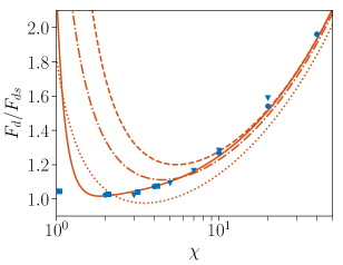
Figure 2: Drag on a finite-length cylinder aligned with the flow direction, normalized by the drag $F_{ds}$ of a sphere of same volume. Dotted, dash-dotted and dashed lines: predictions of $2^{nd}$-, $3^{rd}$- and $4^{th}$-order slender-body approximations, respectively; solid line: semiempirical formula (1); $\bullet$: numerical results of [26]; $\blacksquare$: experimental results of [27]; $\blacktriangledown$: present numerical results for $\text{Re}=0.05$.

Figure 2 displays the drag force $F_{d}\equiv\bf{F}\cdot\bf{e_{x}}$ on the body, normalized by the force $F_{ds}$ on a sphere of same volume (i.e. with diameter $\mathfrak{D}/D=\left(\frac{3}{2}\raisebox{1.5pt}{$\chi$})^{1/3}\right)$), as a function of $\chi$. Clearly, the second-order slender-body approximation (see appendix B) is quite inaccurate, even for large aspect ratios. The third-order approximation provides a better agreement, but significant deviations ($>5\%$) still exist for $\raisebox{1.5pt}{$\chi$}=20$. The fourth-order approximation computed in appendix B approaches the experimental and numerical results down to $\raisebox{1.5pt}{$\chi$}\approx 10$ significantly better. However, all slender-body approximations inherently diverge when $\raisebox{1.5pt}{$\chi$}\rightarrow 1/2$. Actually, Fig. 2 indicates that they are all inaccurate for $\raisebox{1.5pt}{$\chi$}\lesssim 5$; the higher the order of the expansion the larger the aspect ratio below which the slender-body approximation becomes inaccurate. To extend the domain of validity of the theoretical approximation towards short cylinders, we empirically correct the fourth-order approximation by introducing an ad hoc additional term. This term must attenuate the divergence of the slender-body approximation for $\raisebox{1.5pt}{$\chi$}\rightarrow 1/2$ and become negligible for $\raisebox{1.5pt}{$\chi$}=\mathcal{O}(10)$. Therefore we sought it in the form $\raisebox{1.5pt}{$\chi$}^{1/3}(\raisebox{1.5pt}{$\chi$}-1/2)^{-p}$, in such a way that only a $(\raisebox{1.5pt}{$\chi$}-1/2)^{-p}$ correction is introduced in the normalized force $F_{d}/F_{ds}$. The best fit with experimental and numerical data in the range $2\leq\raisebox{1.5pt}{$\chi$}\leq 10$ is obtained with $p=1.75$, a $\pm 3\%$-difference on $p$ leading to a significantly poorer agreement.

The full expression for the drag force incorporating this empirical term then reads

$$F_{d}^{Re=0}\approx 2\pi\mu LU\left(\frac{a^{(1)}}{\ln(2\raisebox{1.5pt}{$\chi$})}+\frac{a^{(2)}}{(\ln(2\raisebox{1.5pt}{$\chi$}))^{2}}+\frac{a^{(3)}}{(\ln(2\raisebox{1.5pt}{$\chi$}))^{3}}+\frac{a^{(4)}}{(\ln(2\raisebox{1.5pt}{$\chi$}))^{4}}-\frac{2.4}{\raisebox{1.5pt}{$\chi$}^{2/3}(\raisebox{1.5pt}{$\chi$}-\frac{1}{2})^{1.75}}\right)\,,$$ (1)

with $U=\bf{U}\cdot\bf{e_{x}}$ and the expressions for the $a^{(i)}$ as provided in appendix B. As Fig. 2 shows, the modified drag law fits the numerical and experimental results well for $\raisebox{1.5pt}{$\chi$}\gtrsim 2$. It still diverges for lower $\chi$, but the drag is then close to that experienced by the equivalent sphere ($F_{d}/F_{ds}\leq 1.05$). Present numerical predictions in the range $3\leq\raisebox{1.5pt}{$\chi$}\leq 10$ are also seen to agree well with results available in the literature. The slight deviation observed for $\raisebox{1.5pt}{$\chi$}=20$ is not unexpected. Indeed, the Reynolds number based on the body length is of $\mathcal{O}(1)$ in this case, making inertial corrections to the drag significant (see below).

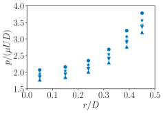
Figure 3: Radial pressure distribution on the upstream end of the cylinder for $\text{Re}=0.05$. $\bullet$: $\raisebox{1.5pt}{$\chi$}=3$; $\star$: $\raisebox{1.5pt}{$\chi$}=5$; $+$: $\raisebox{1.5pt}{$\chi$}=7$; $\blacktriangledown$: $\raisebox{1.5pt}{$\chi$}=10$; $\blacktriangle$: $\raisebox{1.5pt}{$\chi$}=20$. The pressure is assumed to be zero in the far field.

The pressure component to the drag, $F_{dp}$, results from the difference between the pressure distributions on the upstream and downstream ends of the cylinder. Owing to the fore-aft symmetry of the flow in the Stokes regime, these two distributions only differ by the sign of the corresponding pressure, since $p(r,x=L/2)=-p(r,x=-L/2)$. Figure 3 displays the radial pressure distribution on the upstream end. For each $\chi$, the pressure is seen to increase with the distance $r$ to the symmetry axis. At a given radial position, pressure variations are only mildly influenced by the aspect ratio, but this influence becomes larger as the lateral surface is approached.

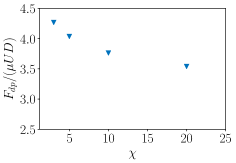
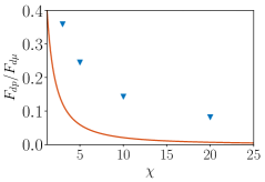
$(a)$                                                    $(b)$

Figure 4: Contributions to the drag force. $(a)$: pressure contribution; $(b)$: ratio of the pressure to the shear stress contributions. $\blacktriangledown$: numerical results for $\text{Re}=0.05$; solid line: low-Re prediction (2) for a prolate spheroid.

Figure 4$(a)$ indicates that $F_{dp}$ only varies weakly with $\chi$. It consistently decreases with the aspect ratio but its variation is less than 20 % from $\raisebox{1.5pt}{$\chi$}=3$ to $\raisebox{1.5pt}{$\chi$}=20$. Figure 4$(b)$ shows the ratio of the pressure contribution to the viscous stress contribution to the drag as a function of $\chi$. This ratio is close to $1/3$ for $\raisebox{1.5pt}{$\chi$}=3$. Then it decreases gradually as $\chi$ increases, and becomes less than $1/10$ for $\raisebox{1.5pt}{$\chi$}=20$. Hence, as expected from purely geometrical considerations, $F_{dp}$ becomes negligible with respect to $F_{d\mu}$ for large $\chi$. It is of some interest to compare this variation with that found for prolate spheroids, namely [28]

$$\frac{F_{dp}}{F_{d\mu}}=\frac{\raisebox{1.5pt}{$\chi$}\ln(\raisebox{1.5pt}{$\chi$}+(\raisebox{1.5pt}{$\chi$}^{2}-1)^{1/2})-(\raisebox{1.5pt}{$\chi$}^{2}-1)^{1/2}}{\raisebox{1.5pt}{$\chi$}^{2}(\raisebox{1.5pt}{$\chi$}^{2}-1)^{1/2}-\raisebox{1.5pt}{$\chi$}\ln(\raisebox{1.5pt}{$\chi$}+(\raisebox{1.5pt}{$\chi$}^{2}-1)^{1/2})}\,.$$ (2)

As Fig. 4$(b)$ indicates, the pressure drag decreases much more slowly with the aspect ratio in the case of a cylindrical body with flat ends. This difference underlines the importance of end effects even for long cylindrical bodies.
Next we consider the influence of inertial effects at low-to-moderate Reynolds number. The slender-body theory initially derived under Stokes flow conditions was extended to small-but-finite Reynolds numbers in [4], still assuming $\text{Re}\ll 1$ but considering that the Reynolds number based on the body length, $\chi$Re, may be arbitrarily large. Lopez and Guazzelli [29] and Roy et al. [30] provided experimental confirmations of the relevance of the finite-Re corrections derived in [4] by examining the settling of long fibers ($10\lesssim\raisebox{1.5pt}{$\chi$}\lesssim 35$) in a Taylor-Green type vortical flow and the sedimentation of isolated fibers with $\raisebox{1.5pt}{$\chi$}=20$ and $100$ in a fluid at rest, respectively. Nevertheless, we are not aware of any detailed validation of the finite-Re theory of [4] in the case of a body aligned with the upstream flow. According to this theory (see also [29] and [30]), the drag force on a long cylindrical body aligned with the flow, disregarding terms of $\mathcal{O}((1/\ln\raisebox{1.5pt}{$\chi$})^{3})$ and higher, reads

$$F_{d}^{\raisebox{1.5pt}{$\chi$}\text{Re}=\mathcal{O}(1)}\approx 2\pi\mu LU\left(\frac{a^{(1)}}{\ln\raisebox{1.5pt}{$\chi$}}+\frac{a^{(2)}-\ln 2+f_{\parallel}}{(\ln\raisebox{1.5pt}{$\chi$})^{2}}\right)\,,$$ (3)

where

$$f_{\parallel}=\frac{1}{2}\left(\frac{E_{1}(\raisebox{1.5pt}{$\chi$}\text{Re})+\ln(\raisebox{1.5pt}{$\chi$}\text{Re})-e^{-\raisebox{1.5pt}{$\chi$}\text{Re}}+\gamma+1}{\raisebox{1.5pt}{$\chi$}\text{Re}}+E_{1}(\raisebox{1.5pt}{$\chi$}\text{Re})+\ln(\raisebox{1.5pt}{$\chi$}\text{Re})+\gamma-2\right)\,,$$ (4)

with $E_{1}(X)=\int_{X}^{+\infty}{\frac{e^{-t}}{t}dt}$ (related to the exponential integral $\text{Ei}(X)$ through $E_{1}(X)=-\text{Ei}(-X)$), and $\gamma$ the Euler constant. In the limit of small $\chi$Re, the inertial correction factor reduces to $f_{\parallel}\approx\frac{1}{8}\raisebox{1.5pt}{$\chi$}\text{Re}$. Note that in (1) and throughout the rest of the paper, the slender-body solution is expanded with respect to $1/\ln(2\raisebox{1.5pt}{$\chi$})$, similar to [1], [3] and [25]. In contrast, an expansion with respect to $1/\ln(\raisebox{1.5pt}{$\chi$})$ was used in [4]. Once truncated at the same order, the two formulations are of course equivalent for $\raisebox{1.5pt}{$\chi$}\gg 2$, but significant differences exist for moderate aspect ratios. This is why we keep the original formulation in (3) and in similar expressions of Sec. IV involving the inertial corrections derived in [4].
The main shortcoming of (3) is obviously the truncation at second order with respect to $1/\ln\raisebox{1.5pt}{$\chi$}$. This limitation is confirmed in Fig. 5, where the influence of inertial effects on the drag force is shown for cylindrical bodies with different aspect ratios. Significant deviations between numerical results and predictions of (3) are observed whatever Re and $\chi$.

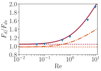
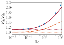
$(a)$                                           $(b)$

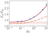
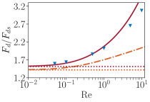
$(c)$                                           $(d)$
$\raisebox{1.5pt}{$\chi$}=3$                                           $\raisebox{1.5pt}{$\chi$}=5$
$\raisebox{1.5pt}{$\chi$}=10$                                         $\raisebox{1.5pt}{$\chi$}=20$

Figure 5: Influence of inertial effects on the drag of finite-length cylinders aligned with the upstream flow. The drag is normalized by that of a sphere of same volume. $\blacktriangledown$: numerical results; solid line: semiempirical prediction (5); dash-dotted line: theoretical prediction (3); dotted line: predictions (1) (upper line) and (3) with $\text{Re}=0$ (lower line).

It is thus desirable to include higher-order corrections with respect to $1/\ln(2\raisebox{1.5pt}{$\chi$})$ to improve the validity of (3). The analysis of [4] was recently extended to third order in [31] using the reciprocal theorem. However, the pre-factor of the third-order term is found in the form of a volume integral to be evaluated in Fourier space. To obtain a more straightforward formula accounting for small-but-finite inertial effects, we use present numerical results to empirically modify (3) by taking advantage of the higher-order corrections present in (1). The best agreement with the numerical results is obtained with the expression

$$F_{d}^{\raisebox{1.5pt}{$\chi$}\text{Re}=\mathcal{O}(1)}\approx 2\pi\mu LU\left[\frac{a^{(1)}}{\ln(2\raisebox{1.5pt}{$\chi$})}+\frac{a^{(2)}+f_{\parallel}}{(\ln(2\raisebox{1.5pt}{$\chi$}))^{2}}+\frac{a^{(3)}+f_{3}f_{\parallel}}{(\ln(2\raisebox{1.5pt}{$\chi$}))^{3}}+\frac{a^{(4)}+f_{4}f_{\parallel}}{(\ln(2\raisebox{1.5pt}{$\chi$}))^{4}}-\frac{2.4}{\raisebox{1.5pt}{$\chi$}^{2/3}(\raisebox{1.5pt}{$\chi$}-\frac{1}{2})^{1.75}}\right]\,,$$ (5)

with $f_{3}=(\raisebox{1.5pt}{$\chi$}\text{Re})^{0.07\chi^{0.5}}$ and $f_{4}=(\raisebox{1.5pt}{$\chi$}\text{Re})^{0.03\chi^{0.9}}$. Predictions of (5) are compared with numerical results in Fig. 5. The agreement is found to be good up to $\text{Re}\approx 1$ whatever the aspect ratio. This is quite remarkable since the derivation of (5) assumes $\text{Re}\ll 1$ (but possibly $\raisebox{1.5pt}{$\chi$}\text{Re}\gtrsim 1$ since $\raisebox{1.5pt}{$\chi$}\gg 1$). Khair and Chisholm [31] also found that their analytical prediction agrees well with the numerically computed drag on a long prolate spheroid up to $\text{Re}\approx 2$ for $\raisebox{1.5pt}{$\chi$}=10$.

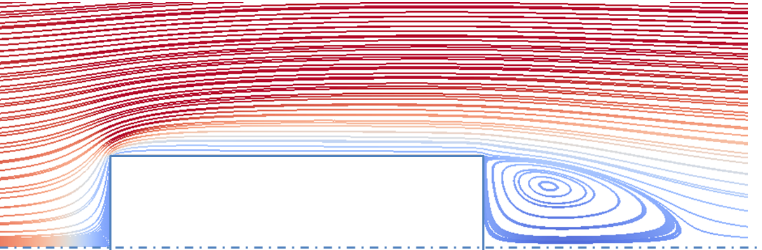
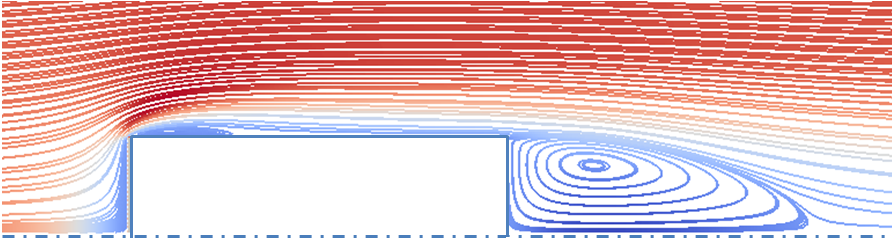
$(a)$                                                                $(b)$

Figure 6: Streamlines pattern for $\raisebox{1.5pt}{$\chi$}=2$ colored with the magnitude of the axial velocity (from $-0.25$ to $1$). $(a)$ $\text{Re}=140$; $(b)$ $\text{Re}=300$.

III.2 From $\mathcal{O}(10)$ to $\mathcal{O}(4\times 10^{2})$ Reynolds numbers

Increasing the Reynolds number, we considered six aspect ratios ranging from $2$ to $10$ and twenty Reynolds numbers from $\text{Re}=20$ to $\text{Re}=400$. The flow past the cylinder was found to reach a steady state in all cases. Nevertheless, the flow structure revealed new features as the Reynolds number increases.
Figure 6$(a)$ displays the streamlines around a cylinder with $\raisebox{1.5pt}{$\chi$}=2$ for $\text{Re}=140$. In this regime, the flow is attached to the body all along the lateral surface but the separation of the boundary layer at the downstream edge results in the generation of a toroidal eddy in the near wake. Simulations indicate that this standing eddy sets in for $\text{Re}\approx 10$ for $\raisebox{1.5pt}{$\chi$}=2$ and $\text{Re}\approx 20$ for $\raisebox{1.5pt}{$\chi$}=7$.

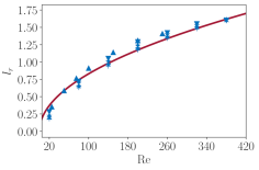
Figure 7: Variation of the length $l_{r}$ of the toroidal eddy vs. the Reynolds number past cylinders with different aspect ratios; $l_{r}$ is measured along the symmetry axis, from the downstream end of the cylinder to the point at which the axial velocity changes sign. $\blacktriangle$: $\raisebox{1.5pt}{$\chi$}=1$ from [23]; $\blacktriangledown$: $\raisebox{1.5pt}{$\chi$}=2$; $\bullet$: $\raisebox{1.5pt}{$\chi$}=3$; $\times$: $\raisebox{1.5pt}{$\chi$}=4$; $\star$: $\raisebox{1.5pt}{$\chi$}=5$; $+$: $\raisebox{1.5pt}{$\chi$}=7$; solid line: $l_{r}(\text{Re})=0.083\text{Re}^{1/2}$.

The length of the standing eddy is plotted in Fig. 7 as a function of the Reynolds number. Remarkably, it is found to be almost independent of $\chi$ and grows approximately as the square root of the Reynolds number.

As the Reynolds number increases, a thin secondary annular eddy sets in along the upstream part of the lateral surface of the body (Fig. 6$(b)$), owing to the detachment of the boundary layer along the upstream edge. The critical Reynolds number $\text{Re}_{c0}$ beyond which this flow pattern is detected is a slowly increasing function of the aspect ratio: from $\text{Re}_{c0}\approx 180$ for $\raisebox{1.5pt}{$\chi$}=2$, to $\text{Re}_{c0}\approx 200$ for $\raisebox{1.5pt}{$\chi$}=5$, $\text{Re}_{c0}\approx 220$ for $\raisebox{1.5pt}{$\chi$}=7$, until $\text{Re}_{c0}\approx 240$ for $\raisebox{1.5pt}{$\chi$}=10$. It will be seen later that this secondary eddy has a strong influence on the viscous friction experienced by the cylinder

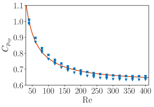
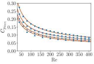
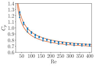
$(a)$                                               $(b)$                                               $(c)$

Figure 8: Pressure drag coefficient $C_{p}$ as a function of Re for different aspect ratios. $(a)$: upstream end; $(b)$: downstream end; $(c)$: sum of the two contributions. $\blacktriangledown$: $\raisebox{1.5pt}{$\chi$}=2$; $\times$: $\raisebox{1.5pt}{$\chi$}=4$; $+$: $\raisebox{1.5pt}{$\chi$}=7$; $\blacktriangle$: $\raisebox{1.5pt}{$\chi$}=10$; solid line in $(a)$: empirical fit (6); solid line in $(b)$: empirical fit (7); solid line in $(c)$: sum (6)+(7) for $\raisebox{1.5pt}{$\chi$}=2$ (upper line) and $\raisebox{1.5pt}{$\chi$}=10$ (lower line).

Figures 8$(a)-(b)$ display the variation with Re of the pressure drag coefficient $C_{p}=8F_{dp}/(\pi\rho D^{2}U^{2})$ on the upstream and downstream ends of the body for various $\chi$. For each aspect ratio, both contributions decrease monotonically with Re. The pressure coefficient on the downstream end ($C_{p_{down}}$) is $3-4$ times smaller than that on the upstream end ($C_{p_{up}}$) for $\text{Re}\approx 100$ and becomes only a small fraction of the latter for $\text{Re}\approx 400$. Moreover, $C_{p_{up}}$ is almost independent of $\chi$ (except for the shortest cylinder), while $C_{p_{down}}$ gradually decreases as the aspect ratio increases. Last, for $\raisebox{1.5pt}{$\chi$}>2$ and $\text{Re}\gtrsim 300$, $C_{p_{up}}$ is seen to tend toward an almost constant value slightly larger than $0.6$. Based on these remarks, approximate expressions for the two contributions take the form

$$C_{p_{up}}(\raisebox{1.5pt}{$\chi$},\text{Re}) \approx 0.62+\frac{11.7}{\text{Re}^{0.9}(1+0.004\text{Re}^{0.9})}$$ (6)

$$C_{p_{down}}(\raisebox{1.5pt}{$\chi$},\text{Re}) \approx 2.05\raisebox{1.5pt}{$\chi$}^{-1/4}\text{Re}^{-1/2}$$ (7)

As Fig. 8$(c)$ confirms, numerical data for the total pressure drag coefficient $C_{p}=C_{p_{up}}+C_{p_{down}}$ are accurately fitted by the sum of (6) and (7).

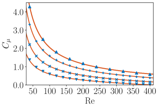
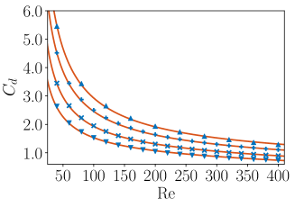
$(a)$                                                            $(b)$

Figure 9: Drag coefficient as a function of Re for different aspect ratios. $(a)$: viscous contribution $C_{\mu}$; $(b)$: total drag coefficient $C_{d}$. $\blacktriangledown$: $\raisebox{1.5pt}{$\chi$}=2$; $\times$: $\raisebox{1.5pt}{$\chi$}=4$; $+$: $\raisebox{1.5pt}{$\chi$}=7$; $\blacktriangle$: $\raisebox{1.5pt}{$\chi$}=10$; for each aspect ratio, the solid lines in $(a)$ and $(b)$ represent the fits (8) and (9), respectively.

Figure 9$(a)$ displays the variation of the viscous drag coefficient, $C_{\mu}(\raisebox{1.5pt}{$\chi$},\text{Re})$. This contribution is seen to be an increasing function of $\chi$. Indeed, the area of the lateral surface of the body may be expressed in the form $\pi D^{2}\raisebox{1.5pt}{$\chi$}$. Hence the normalized viscous force $C_{\mu}=8F_{d\mu}/(\pi\rho D^{2}U^{2})$ is expected to increase almost linearly with the aspect ratio. As usual, $C_{\mu}$ is also a decreasing function of the Reynolds number. However, the observed decrease is much steeper than the classical $\text{Re}^{-1/2}$ behavior expected on the basis of the boundary layer theory. The reason for this stands in the presence of the secondary annular eddy along the lateral surface. The corresponding backflow generates a negative local shear stress which lowers the overall viscous drag. For sufficiently short cylinders and large enough Reynolds numbers, this negative contribution may exceed the positive contribution of the shear stress on the rest of the lateral surface, yielding an overall negative viscous drag. This change of sign takes place at $\text{Re}\approx 420$ for $\raisebox{1.5pt}{$\chi$}=2$. Based on the previous findings, a simple fit for $C_{\mu}$ is found to be

$$C_{\mu}(\raisebox{1.5pt}{$\chi$},\text{Re})\approx 16.45\raisebox{1.5pt}{$\chi$}^{0.7}\text{Re}^{-0.8}+(a_{1}\raisebox{1.5pt}{$\chi$}-a_{2})\text{Re}\,,\quad\mbox{with}\quad a_{1}=4.1\times 10^{-5}\quad\mbox{and}\quad\,a_{2}=6\times 10^{-4}\,.$$ (8)

As Fig. 9$(a)$ shows, the above fit describes the variations of $C_{\mu}$ well throughout the entire range of aspect ratios and Reynolds numbers explored numerically. The last term in the right-hand side of (8) accounts for the influence of the annular eddy. Note that according to (8), the dependence of $C_{\mu}$ with respect to $\chi$ is slightly weaker than expected on the basis of the above simple geometrical argument.
As Figs. 8 and 9 evidence, pressure effects contribute less to the drag than viscous friction for $\text{Re}\lesssim 100$. For Reynolds numbers in the range $100\lesssim\text{Re}\lesssim 300$ and short cylinders ($\raisebox{1.5pt}{$\chi$}\leq 4$), both contributions have a comparable magnitude. However, due to the sharp decrease of the viscous contribution for $\text{Re}\gtrsim 400$ for such short cylinders, the latter eventually becomes smaller than the pressure contribution in the upper part of the Re-range covered by present computations. Adding the approximate expressions (6), (7) and (8), the total drag coefficient is approached as

$$C_{d}(\raisebox{1.5pt}{$\chi$},\text{Re})\approx C_{p_{up}}(\raisebox{1.5pt}{$\chi$},\text{Re})+C_{p_{down}}(\raisebox{1.5pt}{$\chi$},\text{Re})+C_{\mu}(\raisebox{1.5pt}{$\chi$},\text{Re})\,.$$ (9)

As Fig. 9$(b)$ indicates, this fit is in good agreement with the numerically predicted drag throughout the range of $\chi$ and Re covered by the simulations. Note that the upper limit of validity of this fit is presumably $\text{Re}_{max}\approx 400$. In particular, the linear variation of $C_{\mu}$ with Re predicted by (8) cannot continue at very large Reynolds number, as the drag coefficient is expected to decrease with Re for $\text{Re}>\text{Re}_{max}$ and become Re-independent in the limit $\text{Re}\rightarrow\infty$. Conversely, it may be checked that the above fit properly matches the modified low-but-finite $Re$ prediction (5). Consider for instance a cylinder with $\raisebox{1.5pt}{$\chi$}=7$ and $Re=5$. On the one hand, (6)-(9) predict $C_{d}\approx 21.6$ for this set of parameters. On the other hand, according to Fig. 5, the ratio $F_{d}/F_{ds}$ predicted by (5) is approximately $1.85$. Keeping in mind that the diameter $\mathcal{D}$ of the equivalent sphere is related to $D$ through $\mathcal{D}/D=(\frac{3}{2}\raisebox{1.5pt}{$\chi$})^{1/3}$, one has $C_{d}=24\text{Re}^{-1}(\frac{3}{2}\raisebox{1.5pt}{$\chi$})^{1/3}F_{d}/F_{ds}\approx 21.9$. Similarly, for the same Reynolds number but $\raisebox{1.5pt}{$\chi$}=20$, one has $C_{d}\approx 40.7$ from (6)-(9) and $C_{d}\approx 40.3$ from Fig. 5 where $F_{d}/F_{ds}\approx 2.70$. This agreement, which is confirmed with other sets of parameters, allows us to conclude that combining (5) for Reynolds numbers less than a few units with (6)-(9) for larger Re provides an accurate description of drag variations from $\text{Re}=0$ up to $\text{Re}=400$.

IV Forces and torque on a moderately inclined cylinder at low-to-moderate Reynolds number

Figure 10: Schematic of the force components on an inclined cylinder. In this configuration, the inertial torque is negative, tending to rotate the cylinder clockwise.

We now move to the more general configuration in which the cylinder is inclined with respect to the incoming flow by a nonzero angle. For reasons discussed in Sec. I, we limit ourselves to maximum inclinations of $30^{\circ}$. The present section focuses on the low-to-moderate Reynolds number range $[0.1-5]$. Higher Reynolds numbers are considered in the next section.
The nonzero inclination breaks the flow axial symmetry. Therefore, in addition to the force component $F_{\parallel}$ parallel to the cylinder axis, a perpendicular force component ($F_{\perp}$) takes place, together with a spanwise torque ($T$) (Fig. 10). These components are linearly related to the drag and lift forces $F_{d}$ and $F_{l}$, respectively parallel and perpendicular to the incoming velocity U, via the geometric relations

$$F_{\parallel}(\raisebox{1.5pt}{$\chi$},\theta,\text{Re}) = F_{d}(\raisebox{1.5pt}{$\chi$},\theta,\text{Re})\cos\theta-F_{l}(\raisebox{1.5pt}{$\chi$},\theta,\text{Re})\sin\theta\,,$$ (10)

$$F_{\perp}(\raisebox{1.5pt}{$\chi$},\theta,\text{Re}) = F_{l}(\raisebox{1.5pt}{$\chi$},\theta,\text{Re})\cos\theta+F_{d}(\raisebox{1.5pt}{$\chi$},\theta,\text{Re})\sin\theta\,.$$ (11)

In the Stokes regime, the linearity of the loads with respect to the boundary conditions implies that the force acting on the inclined cylinder is linearly related to the drag acting on the same body in the two extreme configurations $\theta=0^{\circ}$ and $\theta=90^{\circ}$ through

$$F_{\parallel}(\raisebox{1.5pt}{$\chi$},\theta) = F_{\parallel}^{\theta=0^{\circ}}(\raisebox{1.5pt}{$\chi$})\cos\theta\,,$$ (12)

$$F_{\perp}(\raisebox{1.5pt}{$\chi$},\theta) = F_{\perp}^{\theta=90^{\circ}}(\raisebox{1.5pt}{$\chi$})\sin\theta\,.$$ (13)

These simple ‘Stokes laws’ are not expected to remain valid when inertial effects become significant. To assess and possibly extend their validity, an approximate expression for $F_{\perp}^{\theta=90^{\circ}}$, similar to (5) for $F_{\parallel}$, is required. In appendix C, we establish the fourth-order slender-body approximation of $F_{\perp}^{\theta=90^{\circ}}(\raisebox{1.5pt}{$\chi$},\text{Re}=0)$, and modify it empirically to extend its validity toward aspect ratios and Reynolds numbers of $\mathcal{O}(1)$. To get some insight into the way inertial effects alter (12)-(13), it is informative to consider the finite-Reynolds-number approximate expressions for $F_{d}$ and $F_{l}$ established for arbitrary inclinations by Khayat and Cox [4]. Evaluating these expressions in the limit $\raisebox{1.5pt}{$\chi$}\text{Re}\ll 1$ and making use of (10)-(11) yields

$$\frac{F_{\parallel}(\raisebox{1.5pt}{$\chi$},\theta,\raisebox{1.5pt}{$\chi$}\text{Re}\ll 1)}{2\pi\mu UL} \approx \left(F_{\parallel}^{*\theta=0^{\circ}}(\raisebox{1.5pt}{$\chi$},\raisebox{1.5pt}{$\chi$}\text{Re}\ll 1)-\frac{1}{16}\sin^{2}\theta\frac{\raisebox{1.5pt}{$\chi$}Re}{(\ln\raisebox{1.5pt}{$\chi$})^{2}}\right)\cos\theta\,,$$ (14)

$$\frac{F_{\perp}(\raisebox{1.5pt}{$\chi$},\theta,\raisebox{1.5pt}{$\chi$}\text{Re}\ll 1)}{4\pi\mu UL} \approx \left(F_{\perp}^{*\theta=90^{\circ}}(\raisebox{1.5pt}{$\chi$},\raisebox{1.5pt}{$\chi$}\text{Re}\ll 1)+\frac{1}{16}\cos^{2}\theta\frac{\raisebox{1.5pt}{$\chi$}Re}{(\ln\raisebox{1.5pt}{$\chi$})^{2}}\right)\sin\theta\,,$$ (15)

where $F_{\parallel}^{*}$ and $F_{\perp}^{*}$ stand for the dimensionless second-order expansion of the corresponding force with respect to $1/\ln\raisebox{1.5pt}{$\chi$}$ in the limit of low-but-finite $\chi$Re, as provided by (3) and (32), respectively. According to (3) and the asymptotic form of the inertial correction $f_{\parallel}$ in the limit $\raisebox{1.5pt}{$\chi$}\text{Re}\rightarrow 0$, one has $F_{\parallel}^{*\theta=0^{\circ}}(\raisebox{1.5pt}{$\chi$},\raisebox{1.5pt}{$\chi$}\text{Re}\ll 1)=[\text{ln}\raisebox{1.5pt}{$\chi$}]^{-1}+(\frac{3}{2}-2\text{ln}2+\frac{1}{8}\raisebox{1.5pt}{$\chi$}\text{Re})[\text{ln}\raisebox{1.5pt}{$\chi$}]^{-2}$. Similarly, (32) and the asymptotic form of $f_{\perp}$ yield $F_{\perp}^{*\theta=0^{\circ}}(\raisebox{1.5pt}{$\chi$},\raisebox{1.5pt}{$\chi$}\text{Re}\ll 1)=[\text{ln}\raisebox{1.5pt}{$\chi$}]^{-1}+(\frac{1}{2}-2\text{ln}2+\frac{1}{4}\raisebox{1.5pt}{$\chi$}\text{Re})[\text{ln}\raisebox{1.5pt}{$\chi$}]^{-2}$. Expressions (14)-(15) indicate that the angular dependence of $F_{\parallel}$ and $F_{\perp}$ becomes more complex in the presence of inertial effects, involving higher-order harmonics of $\theta$. Moreover they suggest that the $\theta$-dependent inertial corrections tend to decrease $F_{\parallel}$ and increase $F_{\perp}$, compared to the prediction of the extrapolated ‘Stokes law’ based on the finite-Re drag forces $F_{\parallel}^{*\theta=0^{\circ}}$ and $F_{\perp}^{*\theta=90^{\circ}}$.

Still in the Stokes regime, the spanwise torque is zero whatever $\theta$, owing to the geometrical symmetries of the cylinder and the reversibility of Stokes equations. However, nonlinearities inherent to inertial effects result in a finite torque. In the limit $Re\raisebox{1.5pt}{$\chi$}\ll 1$, the finite-Reynolds-number expression for this torque obtained in [4] reduces to

$$\frac{T(\raisebox{1.5pt}{$\chi$},\theta,\raisebox{1.5pt}{$\chi$}\text{Re}\ll 1)}{\mu U(L/2)^{2}}\approx-\frac{5\pi}{12}\frac{\raisebox{1.5pt}{$\chi$}Re}{(\ln\raisebox{1.5pt}{$\chi$})^{2}}\sin 2\theta\,.$$ (16)

This negative torque tends to rotate the cylinder perpendicular to the flow direction.
In what follows we make use of the numerical results to examine the validity of ‘Stokes laws’ (12)-(13) and of the predictions of [4] for low-to-moderate Reynolds numbers.

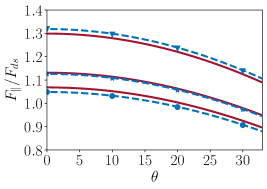
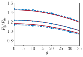
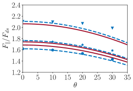
$(a)$                                         $(b)$                                         $(c)$
$\text{Re}=0.1$                                 $\text{Re}=0.5$                                 $\text{Re}=5$

Figure 11: Parallel force component $F_{\parallel}$ vs. the inclination angle $\theta$ for $\bullet$: $\raisebox{1.5pt}{$\chi$}=3$, $\star$: $\raisebox{1.5pt}{$\chi$}=5$, $\blacktriangledown$: $\raisebox{1.5pt}{$\chi$}=10$. Dashed line: prediction (12) based on the numerical value of $F_{\parallel}^{\theta=0^{\circ}}$; solid line: prediction (12) based on the semiempirical approximation (5) for $F_{\parallel}^{\theta=0^{\circ}}$.

Figure 11 displays the parallel force component $F_{\parallel}$ for three Reynolds numbers and aspect ratios $\raisebox{1.5pt}{$\chi$}=3,\,5$ and $10$, respectively. At the lower two Re, variations of $F_{\parallel}$ closely follow the $\cos\theta$-behavior predicted by (12) whatever the aspect ratio. This implies that the $\sin^{2}\theta$-inertial correction in (14) has only a marginal influence at moderate inclinations for $\raisebox{1.5pt}{$\chi$}\text{Re}\lesssim 5$. Indeed, for $\theta=30^{\circ}$, this correction is less that $2\%$ of $F_{\parallel}^{*\theta=0^{\circ}}$ whatever the aspect ratio. However, the inertial correction included in $F_{\parallel}^{*}$ reaches $16\%$ for $\raisebox{1.5pt}{$\chi$}=10$, indicating that inertial effects are already significant. In other words, in the range of moderate inclinations considered here, the ‘Stokes law’ still accurately predicts $F_{\parallel}(\raisebox{1.5pt}{$\chi$},\theta,\text{Re})$ for $\text{Re}\lesssim 1$, provided the prediction makes use of the inertia-corrected drag $F_{\parallel}^{\theta=0^{\circ}}(\raisebox{1.5pt}{$\chi$},\text{Re})$.
At $\text{Re}=5$, influence of inertial effects has become dominant. Since the magnitude of $\theta$-dependent inertial correction also increases with Re$\chi$, the larger the aspect ratio the stronger these effects at a given Re. This may be appreciated in Fig. 11$(c)$, where the difference between the computed force and the prediction of the ‘Stokes law’ is seen to increase significantly with $\chi$ for $\theta>10^{\circ}$, from less than $2\%$ for $\raisebox{1.5pt}{$\chi$}=3$ at $\theta=30^{\circ}$ to $9\%$ for $\raisebox{1.5pt}{$\chi$}=10$ at the same inclination. Interestingly, the under-prediction of $F_{\parallel}$ by the Stokes law is at odds with the low-$\chi$Re prediction (14) which suggests that this ‘law’ should overestimate $F_{\parallel}$, since it ignores the negative $\sin^{2}\theta$-inertial contribution. This contradiction emphasizes the fact that the $\theta$-dependences of inertial effects in the low-$\chi$Re range and in the range $10\lesssim\raisebox{1.5pt}{$\chi$}\text{Re}\lesssim 10^{2}$ are drastically different.

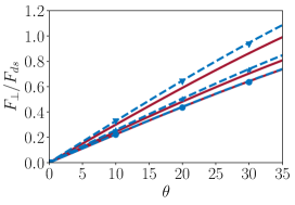
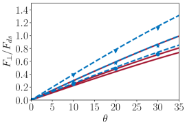
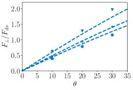
$(a)$                                         $(b)$                                         $(c)$
$\text{Re}=0.1$                                 $\text{Re}=0.5$                                 $\text{Re}=5$

Figure 12: Perpendicular force component $F_{\perp}$ as a function of $\theta$ for $\bullet$: $\raisebox{1.5pt}{$\chi$}=3$, $\star$: $\raisebox{1.5pt}{$\chi$}=5$, $\blacktriangledown$: $\raisebox{1.5pt}{$\chi$}=10$. Solid line: ‘Stokes law’ (13) based on the semiempirical creeping-flow estimate (31) for $F_{\perp}^{\theta=90^{\circ}}(\raisebox{1.5pt}{$\chi$})$; dashed line: same with $F_{\perp}^{\theta=90^{\circ}}$ based on the semiempirical finite-Re estimate (34). In $(a)$, the two estimates overlap for $\raisebox{1.5pt}{$\chi$}=3$; in $(b)$, the prediction for $\raisebox{1.5pt}{$\chi$}=10$ based on (31) overlaps with that for $\raisebox{1.5pt}{$\chi$}=5$ based on (34).

Figure 12 shows the variations of the perpendicular force component in the same low-to-moderate Re-range. At $\text{Re}=0.1$ (Fig. 12$(a)$), $F_{\perp}$ is accurately approximated for the two cylinders with $\raisebox{1.5pt}{$\chi$}=3$ and $\raisebox{1.5pt}{$\chi$}=5$ by the ‘Stokes law’ based on the creeping-flow prediction (31) for $F_{\perp}^{\theta=90^{\circ}}(\raisebox{1.5pt}{$\chi$})$. This is no longer the case for $\raisebox{1.5pt}{$\chi$}=10$, where a significant underestimate may be noticed. In this case, the length-based Reynolds number $\chi$Re is unity, implying that inertial effects are already significant. This is why the Stokes law based on the composite expression (34) for $F_{\perp}^{\theta=90^{\circ}}$, which incorporates the inertial correction derived in [4], closely approaches the numerical data set. The validity of the Stokes law based on (34) is maintained for $\text{Re}=0.5$ whatever the aspect ratio. For $\text{Re}=5$ (Fig. 12$(c)$), predictions of the same law are found to deviate significantly from numerical results, overestimating $F_{\perp}$ by more than $10\%$ for $\raisebox{1.5pt}{$\chi$}=3$ and underestimating it by a similar percentage for $\raisebox{1.5pt}{$\chi$}=10$. This is no surprise, since the inertial corrections involved in (34) are based on the finite-Re theory of [4] which assumes $\text{Re}\ll 1$. In this respect, the deviations observed in Fig. 12$(c)$ may even be considered as surprisingly small.
Variations of the spanwise torque with $\raisebox{1.5pt}{$\chi$},\,\theta$ and Re are displayed in Fig. 13. As expected, the torque is negative, tending to orient the cylinder broadside on. Variations with the cylinder inclination closely follow the $\sin 2\theta$-dependence predicted in the low-$\chi$Re limit by (16). The magnitude of the torque increases with the Reynolds number, in line with its inertial nature. For a given Re, the shorter the cylinder the stronger the normalized torque. Numerical results are compared with the full theoretical prediction of Khayat and Cox [4], namely

$$\frac{T(\raisebox{1.5pt}{$\chi$},\theta,\text{Re}\ll 1)}{\mu U(L/2)^{2}} = \frac{2\pi}{(\ln{\raisebox{1.5pt}{$\chi$}})^{2}}\left\{\cos\theta\left[\mathcal{Z}(X)-\frac{E_{1}(X)+\ln X+\gamma}{X}+\mathcal{Z}(Y)-\frac{E_{1}(Y)+\ln Y+\gamma}{Y}\right]\right.$$ (17)

$$\bigg{.}\frac{}{}+\mathcal{Z}(Y)-\mathcal{Z}(X)\bigg{\}}\sin\theta+\mathcal{O}\left(\frac{1}{(\ln{\raisebox{1.5pt}{$\chi$}})^{3}}\right)\,,$$

where $\mathcal{Z}(X)=\frac{2}{X}\left(1+\frac{e^{-X}-1}{X}\right)$, $X=\frac{1}{2}\raisebox{1.5pt}{$\chi$}\text{Re}(1-\cos\theta)$, $Y=\frac{1}{2}\raisebox{1.5pt}{$\chi$}\text{Re}(1+\cos\theta)$ and $E_{1}$ and $\gamma$ as defined in (4). According to Fig. 13, this prediction closely approaches the numerical results for the longest cylinder up to Re=0.5, together with those for the intermediate cylinder at $\text{Re}=0.1$. It is no surprise that the low-but-finite Re theory is unable to provide a reasonable prediction for any of the three cylinders at $\text{Re}=5$. In their experiments, Roy et al. [30] considered cylindrical fibers with $\text{Re}\approx 0.15$. With $\raisebox{1.5pt}{$\chi$}=20$ they found the theory of [4] to over-predict the torque by more than $20\%$ for $\raisebox{1.5pt}{$\chi$}=20$ at $\theta=30^{\circ}$, and to slightly under-predict it (by $7-8\%$) for $\raisebox{1.5pt}{$\chi$}=100$. Present results provide a stronger support to the theory, since the difference observed in Fig. 13$(a)$ is only of the order of $5\%$ for $\raisebox{1.5pt}{$\chi$}=10$ and clearly decreases with increasing $\chi$. The fact that the asymptotic prediction, in which terms of $\mathcal{O}\left((\ln{\raisebox{1.5pt}{$\chi$}})^{-3}\right)$ are neglected, correctly estimates the torque on a $\raisebox{1.5pt}{$\chi$}=5$ cylinder at $\text{Re}=0.1$ but not at $\text{Re}=0.5$, while it still provides an accurate prediction at the same Reynolds number for $\raisebox{1.5pt}{$\chi$}=10$ is noticeable. It suggests that the conditions $\text{Re}\ll 1$ and $\raisebox{1.5pt}{$\chi$}\gg 1$ on which the asymptotic prediction is grounded must rather been understood as $\text{Re}\ll 1$ and $\text{Re}/\raisebox{1.5pt}{$\chi$}^{2}\ll 1$. Indeed, the ratio $\text{Re}/\raisebox{1.5pt}{$\chi$}^{2}$ stands below $0.005$ in all three configurations correctly predicted by (17), while it is beyond $0.01$ in all other cases. For practical purposes, we sought an empirical fit of the torque valid for long enough cylinders and reducing to (16) (the limit form of (17)) for $\raisebox{1.5pt}{$\chi$}\text{Re}\rightarrow 0$. As all three panels in Fig. 13 indicate, numerical data corresponding to $\raisebox{1.5pt}{$\chi$}=10$ and $\raisebox{1.5pt}{$\chi$}=5$ are accurately approached by the formula

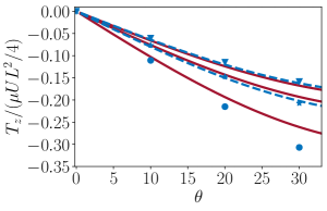
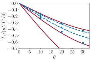
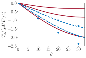
$(a)$                                         $(b)$                                         $(c)$
$\text{Re}=0.1$                                    $\text{Re}=0.5$                                    $\text{Re}=5$

Figure 13: Torque as a function of $\theta$ for $\bullet$: $\raisebox{1.5pt}{$\chi$}=3$, $\star$: $\raisebox{1.5pt}{$\chi$}=5$, $\blacktriangledown$: $\raisebox{1.5pt}{$\chi$}=10$. Solid line: asymptotic prediction (17) for low-but-finite Re; dashed line: approximate fit (18) for $\raisebox{1.5pt}{$\chi$}=5$ and $10$.

$$\frac{T(\raisebox{1.5pt}{$\chi$}\gg 1,\theta,\text{Re})}{\mu U(L/2)^{2}}\approx-\frac{5\pi}{12}\frac{\text{Re}}{(1+\raisebox{1.5pt}{$\chi$}\text{Re}^{1.1})^{0.5}}\left\{\frac{\raisebox{1.5pt}{$\chi$}}{(\ln\raisebox{1.5pt}{$\chi$})^{2}}+\frac{13.5-30\,\text{Re}^{1/2}}{\raisebox{1.5pt}{$\chi$}(\ln\raisebox{1.5pt}{$\chi$})^{3}}e^{-0.7\text{Re}}\right\}\sin 2\theta\,.$$ (18)

The $\mathcal{O}\left(\raisebox{1.5pt}{$\chi$}^{-1}(\ln{\raisebox{1.5pt}{$\chi$}})^{-3}\right)$-term only provides a marginal contribution for $\raisebox{1.5pt}{$\chi$}=10$. Consequently the leading-order $\mathcal{O}\left(\raisebox{1.5pt}{$\chi$}(\ln{\raisebox{1.5pt}{$\chi$}})^{-2}\right)$-truncation of (18) is sufficient to correctly estimate the torque on cylindrical fibers with $\raisebox{1.5pt}{$\chi$}\gtrsim 10$ up to $\text{Re}=5$. A correction proportional to $(\ln{\raisebox{1.5pt}{$\chi$}})^{-4}$ may certainly be incorporated in (18) to properly estimate the torque on very short cylinders.

V Fully inertial stationary regime

As pointed out in Sec. III.2, the flow past a cylinder aligned with the incoming velocity is stationary and axisymmetric within the full range of Re investigated here. Although the axial symmetry breaks down when $\theta$ is nonzero, the flow remains stationary up to a critical Reynolds number, $\text{Re}_{c}(\raisebox{1.5pt}{$\chi$},\,\theta)$, larger than $300$. Details on the first unsteady regimes that take place beyond this threshold are provided as Supplemental Material. Here we concentrate on the stationary non-axisymmetric regime extending from Reynolds numbers of $\mathcal{O}(10)$ up to $\text{Re}_{c}$. To limit the computational cost, simulations in this regime were only carried out for cylinders with aspect ratios $\raisebox{1.5pt}{$\chi$}=3,5$ and $7$. However, the results to be discussed hereinafter suggest that the flow structure and loads are only weakly affected by finite-length effects beyond $\raisebox{1.5pt}{$\chi$}\approx 5$ in this range of Reynolds number, although the inertial load coefficients defined below may well continue to depend on $\chi$, even for $\raisebox{1.5pt}{$\chi$}\gg 1$. Consequently, the physical phenomena involved and the simulation-based approximate expressions for the loads provided below are expected to apply without significant changes to cylinders with $\raisebox{1.5pt}{$\chi$}\gg 1$, which makes them relevant to analyze the motion of long cylindrical fibers in inertia-dominated regimes.
In Sec. III.2, we showed that, for Reynolds numbers of $\mathcal{O}(10^{2})$, the flow structure past a cylinder aligned with the incoming velocity exhibits the presence of a thin annular standing eddy along the upstream part of the lateral surface. This feature was found to significantly influence the drag force, being able to change the sign of the viscous drag for sufficiently short cylinders and large Reynolds numbers. The situation is qualitatively similar in the $(\theta,\,\text{Re})$-range considered hereinafter since, for large enough inclinations and Reynolds numbers, the flow field exhibits specific features which directly affect the loads on the body. Consequently, it is relevant to examine first how the flow close to the body varies with the control parameters, which is the purpose of Sec. V.1. Then, the possibility to use numerical data to derive simple laws for the force components is considered in Sec. V.2, before empirical fits for the axial force and spanwise torque are built in Sec. V.3.

 
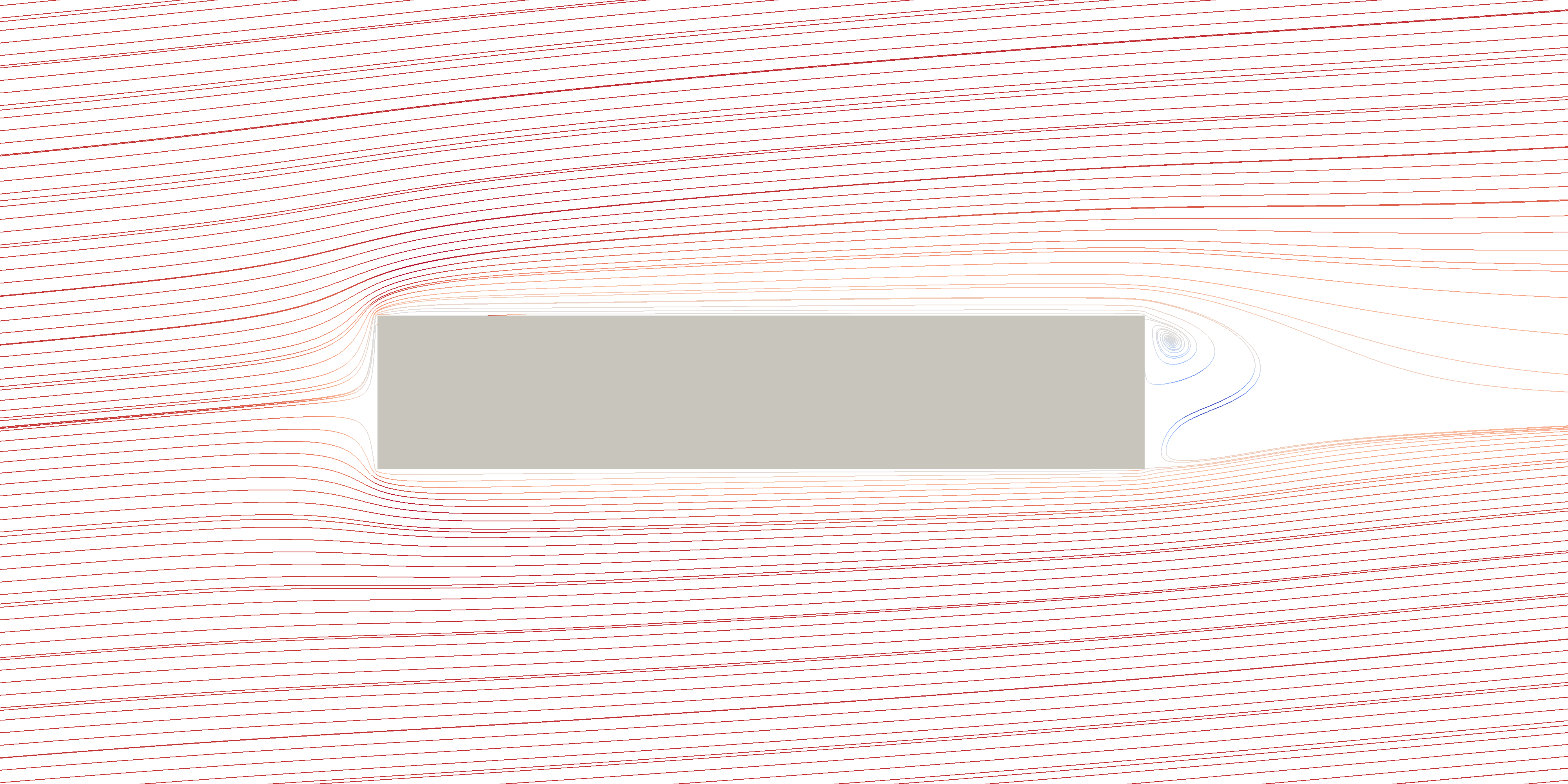
$S^{-}$
$fs^{-}$
$(a)$                                                            $(b)$
 
$fs^{+}$
$E$
$S^{+}$       A
$fs^{-}$
                                           $\mathcal{R}_{b}$
                                             $S^{+}$        A
                                           $\mathcal{R}_{f}$
$(c)$                                                            $(d)$
 
$fs^{+}$
$E$
$S^{+}$        A
$fs^{-}$
                                           $\mathcal{R}_{b}$
                                               $S^{+}$           A
                                           $\mathcal{R}_{f}$
$(e)$                                                            $(f)$

Figure 14: Streamlines in the symmetry plane $z=0$ (left) and in the plane $y=D/2$ tangent to the lateral surface along the top generatrix (right) for a cylinder with $\raisebox{1.5pt}{$\chi$}=5$ at $\text{Re}=140$. Streamlines are colored according to the magnitude and sign of the axial velocity from $-0.25$ (deep blue) to $+1$ (deep red). $(a)-(b)$: $\theta=5^{\circ}$; $(c)-(d)$: $\theta=15^{\circ}$; $(e)-(f)$: $\theta=30^{\circ}$.

V.1 Flow structure

Throughout the regime under consideration, the flow field exhibits a mirror symmetry with respect to the $(x,y)$-plane which contains both the body axis and the incoming velocity. Figure 14 helps to understand how the flow structure past the cylinder varies with the inclination angle. Several generic features emerge. First, the front stagnation point standing in the symmetry plane $z=0$ is seen to move downward (i.e. toward negative $y$) as $\theta$ increases, almost reaching the bottom generatrix ($y=-D/2)$ for $\theta=30^{\circ}$ whatever Re. At the back of the body, the fluid that has passed over the upper part of the lateral surface is entrained downwards. It recirculates toward the downstream end within a region whose length in the streamwise $(x)$ direction is typically of the order of the cylinder radius for $\text{Re}=140$. Examination of this recirculating region at other Reynolds numbers (not shown) indicates that its length increases gradually with Re, becoming of the order of $D$ for $\text{Re}=300$. Unlike the standing eddy existing in the axisymmetric configuration (Sec. III.2), this recirculating zone is no longer a closed toroid. Indeed, once the fluid entrained downward gets very close to the lowest generatrix (point $S^{-}$ in Fig. 14$(a)$), it is expelled downstream in the main flow, just above the open streamline $fs^{-}$ emanating from $S^{-}$. Out of the symmetry plane, the three-dimensional streamlines displayed in Fig. 15 (for $\text{Re}=300$, to magnify the regions in which the fluid recirculates) reveal that fluid particles entrapped in the recirculating region describe successive loops before being sucked into the wake and advected downstream. This scenario is similar to that observed in [32] at the back of a sphere in the first (steady) non-axisymmetric wake regime.

For $\text{Re}=140$ and $\theta=5^{\circ}$ (Fig. 14$(a)$), the flow along the body remains attached everywhere to the lateral surface. The lower (resp. higher) the Reynolds number, the larger (resp. smaller) the critical inclination at which separation occurs along the upper part of this surface. For instance, the flow is still unseparated at $\theta=15^{\circ}$ for $\text{Re}=40$ but is already separated at $\theta=5^{\circ}$ for $\text{Re}=300$. Separation starts at the intersection of the upstream end and the upper generatrix (point $S^{+}$ in Figs. 14$(c)-(f)$). Beyond the corresponding critical $\theta$ and/or Re, separation takes place over an open surface of finite extent, the most downstream point of which (point $A$ in Figs. 14$(c)-(f)$) stands on the symmetry plane. Still in the plane $y=D/2$, the separating line starting at $A$ develops upstream on the sides of the cylinder (regions $\mathcal{R}_{b}$ and $\mathcal{R}_{f}$ in Figs. 14$(d)$ and $(f)$) before joining the incoming flow. Not visible in Fig. 14, the lower part of the separation surface ($y<D/2$) on the sides of the cylinder exhibits a structure qualitatively similar to that of regions $\mathcal{R}_{b}$ and $\mathcal{R}_{f}$ and ends in some intermediate plane $0<y<D/2$, the position of which depends on $\theta$ and Re. Moving away from the lateral surface above the upper generatrix ($y>D/2$), the extent of the separation surface in the spanwise direction decreases gradually until its trace reduces to a single point some distance above the cylinder. This apex (point $E$ in Figs. 14$(c)$ and $(e)$) looks like the ‘eye of the storm’ of the separated region. The larger $\theta$ and Re, the larger the distance between points $S^{+}$ and $E$ in both the $x$- and $y$-directions. Fluid is brought in the neighborhood of $E$ from both sides of the cylinder in a way similar to that observed in Figs. 14$(d)$ and $(f)$ in the plane $y=D/2$ (see Fig. 15). Then it is sent back toward the upstream end in between the ‘eye’ and the cylinder. The dividing streamline joining the region of the ‘eye’ to point $A$ gets very close to the uppermost point $S^{+}$ of the upstream end. There, fluid particles are deviated by the ‘fresh’ fluid flowing along the free streamline $fs^{+}$ and advected downstream, just below this free streamline. Streamlines that pass closer to to the ‘eye’ stay further away from the cylinder surface within the recirculating region. Consequently they also stay further away from $fs^{+}$ once they escape this region, the corresponding fluid filling the intermediate region in between $fs^{+}$ and the cylinder at the back of the separation surface. Overall, the flow past the cylinder looks massively separated in between the free streamlines $fs^{-}$ and $fs^{+}$, the position of the ‘eye’ governing the flow structure in the intermediate region. A similar open separation configuration was recently observed over inclined prolate spheroids in the range $5\leq\text{Re}\leq 100$ in [33].

Figure 15: Three-dimensional streamlines past an inclined cylinder with $\raisebox{1.5pt}{$\chi$}=5$, $\theta=15^{\circ}$ and $\text{Re}=300$.

V.2 Are ‘Stokes laws’ valid for inclined cylinders at moderate-to-large Reynolds number?

We now make use of the numerical results to build approximate force and torque laws valid for $|\theta|\lesssim 30^{\circ}$ and $\text{Re}\gtrsim 10$ in the stationary non-axisymmetric flow regime. For this purpose, we characterize the force components through the parallel and perpendicular force coefficients defined via the identify $(F_{\perp},F_{\parallel})\equiv(C_{\perp},C_{\parallel})\rho U^{2}LD/2$. Similarly, we introduce the torque coefficient $C_{t}$ related to the spanwise torque $T$ through $T\equiv C_{t}\rho U^{2}L^{2}D$.

To assess the validity of the ‘Stokes laws’ in this regime, we inject the numerical results in (10)-(11) and compare the resulting $C_{\parallel}(\raisebox{1.5pt}{$\chi$},\theta,\text{Re})$ and $C_{\perp}(\raisebox{1.5pt}{$\chi$},\theta,\text{Re})$ with the predictions of (12)-(13) at the relevant Reynolds number and aspect ratio. To achieve this comparison, the two coefficients $C_{\parallel}^{\theta=0^{\circ}}$ and $C_{\perp}^{\theta=90^{\circ}}$ are required for every value of $\chi$ and Re. $C_{\parallel}^{\theta=0^{\circ}}(\raisebox{1.5pt}{$\chi$},\text{Re})$ is directly related to the drag determined in Sec. III up to a normalization factor. More specifically, in the Re-range considered in Sec. III.2, $C_{\parallel}$ and the drag coefficient $C_{d}$ resulting from (6)-(9) are linked through the relation $C_{\parallel}^{\theta=0^{\circ}}(\raisebox{1.5pt}{$\chi$},\text{Re})=\frac{\pi}{4}\raisebox{1.5pt}{$\chi$}^{-1}C_{d}(\raisebox{1.5pt}{$\chi$},\text{Re})$. At lower Reynolds number, $C_{\parallel}^{\theta=0^{\circ}}$ is readily obtained through the approximate expression (5) as $C_{\parallel}^{\theta=0^{\circ}}(\raisebox{1.5pt}{$\chi$},\text{Re})=4\pi\text{Re}^{-1}\mathcal{F}(\raisebox{1.5pt}{$\chi$},\text{Re})$, where $\mathcal{F}(\raisebox{1.5pt}{$\chi$},\text{Re})$ denotes the quantity within brackets in (5). A direct graphical estimate of $\mathcal{F}(\raisebox{1.5pt}{$\chi$},\text{Re})$ is provided for several aspects ratios in Fig. 5, noting that the relation between $\mathcal{F}(\raisebox{1.5pt}{$\chi$},\text{Re})$ and the normalized drag $F_{d}/F_{ds}$ is $\mathcal{F}(\raisebox{1.5pt}{$\chi$},\text{Re})=\left(\frac{81}{16}\raisebox{1.5pt}{$\chi$}^{-2}\right)^{1/3}F_{d}/F_{ds}$.
Since we did not compute the loads on a cylinder held perpendicular to the flow, we use data from the literature to estimate $C_{\perp}^{\theta=90^{\circ}}(\raisebox{1.5pt}{$\chi$},\text{Re})$. A large number of experimental data obtained with long cylinders was compiled in [34]. The corresponding curves for the drag per unit length were fitted in [24] in the form

$$C_{\perp}^{\theta=90^{\circ}}(\raisebox{1.5pt}{$\chi$}\gg 1,\text{Re})\approx 9.69\text{Re}^{-0.78}(1+a\text{Re}^{n})\,,$$ (19)

with $a=0.227$ and $n=0.55$ for $5<\text{Re}\leq 40$, and $a=0.084$ and $n=0.82$ for $40<\text{Re}\leq 400$, respectively. Comparisons between predictions of (19) and experimental results from [35] for finite-length cylinders falling perpendicular to their axis indicate that the drag is only marginally affected by end effects as soon as $\raisebox{1.5pt}{$\chi$}\gtrsim 2$ and $\text{Re}\gtrsim 10$ [24]. This is why we consider that (19) provides a relevant estimate of $C_{\perp}^{\theta=90^{\circ}}(\raisebox{1.5pt}{$\chi$},\text{Re})$ throughout the range of aspect ratios and Reynolds numbers of interest here.
The resulting comparison between numerical results and predictions of (12)-(13) is presented in Fig. 16. The parallel force coefficients are seen to decrease significantly as $\chi$ increases. In Sec. III, where the drag was normalized using the frontal area $\pi D^{2}/4$, we found that the pressure contribution to the drag in the configuration $\theta=0^{\circ}$ is almost independent of $\chi$. For this reason, the corresponding contribution to $C_{\parallel}^{\theta=0^{\circ}}(\raisebox{1.5pt}{$\chi$},\text{Re})$, which involves a normalization by $LD$, behaves as $\raisebox{1.5pt}{$\chi$}^{-1}$ and is responsible for the most part of the large variations of $C_{\parallel}(\raisebox{1.5pt}{$\chi$},\theta,\text{Re})$ with $\chi$ observed in Figs. 16$(a),(c),(e)$. Variations of $C_{\parallel}$ with $\theta$ are remarkable in that they clearly contradict the ‘Stokes law’. Indeed, it is seen that $C_{\parallel}$ is almost independent of $\theta$ for $\text{Re}=20$ (apart from a modest decrease at $\theta=30^{\circ}$ for $\raisebox{1.5pt}{$\chi$}=3$), while it increases with the cylinder inclination for larger Reynolds numbers. Still modest for $\text{Re}=80$, this increase makes $C_{\parallel}$ $40-50\%$ larger for $\theta=30^{\circ}$ than for $\theta=0^{\circ}$ at $\text{Re}=300$. Clearly the ‘Stokes law’ (12) is unable to reproduce the observed trends.

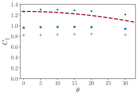
$(a)$	$(b)$
$\text{Re}=20$	$\text{Re}=20$

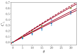
$(c)$	$(d)$
$\text{Re}=80$	$\text{Re}=80$

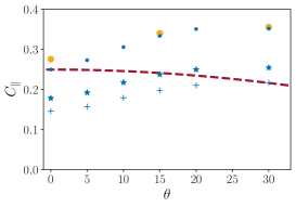
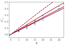
$(e)$	$(f)$
$\text{Re}=300$	$\text{Re}=300$

Figure 16: Parallel and perpendicular force coefficients ($C_{\parallel},C_{\perp}$ ) vs. $\theta$ for $\bullet$: $\raisebox{1.5pt}{$\chi$}=3$, $\star$: $\raisebox{1.5pt}{$\chi$}=5$, +: $\raisebox{1.5pt}{$\chi$}=7$. Dashed lines: ‘Stokes laws’ (12)-(13) based on the value of $C_{\parallel}^{\theta=0^{\circ}}(\raisebox{1.5pt}{$\chi$}=3)$ and $C_{\perp}^{\theta=90^{\circ}}(\raisebox{1.5pt}{$\chi$}\gg 1)$ at the relevant Reynolds number; solid line: approximate fit (20). The yellow bullets in panels $(c)-(d)$ and $(e)-(f)$ refer to the results of [13] for $\raisebox{1.5pt}{$\chi$}=3$ at $\text{Re}=75$ and $250$, respectively.

The situation is markedly different with the perpendicular force coefficient, which is found to follow closely the $\sin\theta$-dependence predicted by (13) throughout the entire range of $\theta$ and Re. Moreover, $C_{\perp}$ only mildly varies with the aspect ratio, with less than $20\%$ differences between the shortest and longest cylinders whatever Re (Figs. 16$(b),(d),(f)$). However, it is also clear from these panels that the predictions of (13) based on the expression (19) for $C_{\perp}^{\theta=90^{\circ}}(\raisebox{1.5pt}{$\chi$}\gg 1,\text{Re})$ over-predict $C_{\perp}(\raisebox{1.5pt}{$\chi$},\theta,\text{Re})$ for the highest two Reynolds numbers, the overestimate increasing with Re. This is actually no surprise, since in the Re-range considered here, the flow structure past an inclined cylinder with $0^{\circ}\leq\theta\leq 30^{\circ}$ has little in common with that past a cylinder held perpendicular to the incoming velocity. While the wake of the latter becomes unsteady for $\text{Re}\approx 47$ and three-dimensional for $\text{Re}\approx 180$ [11], all inclined configurations considered here are stationary and inherently three-dimensional. Therefore, the connection between the two configurations becomes loose beyond Reynolds numbers of a few tens. Nevertheless, to keep the advantage of (13) which is asymptotically correct in the creeping-flow limit, we sought an empirical Re-dependent correction capable of properly approaching the numerical results while vanishing for both $\text{Re}\rightarrow 0$ and $\theta=90^{\circ}$. We sought another correction to account for the dependence of $C_{\perp}$ with respect to the aspect ratio, requesting that this correction also vanishes for $\theta=90^{\circ}$ for the aforementioned reasons. Ideally, one would like this correction to recover the proper behavior $C_{\perp}\propto\text{Re}^{-1}(\ln\raisebox{1.5pt}{$\chi$})^{-1}$ for $\text{Re}\rightarrow 0$. However, due to the singular nature of the problem in the limit $\text{Re}\rightarrow 0,\,\raisebox{1.5pt}{$\chi$}\rightarrow\infty$ (Stokes paradox), it is known that $C_{\perp}^{\theta=90^{\circ}}(\raisebox{1.5pt}{$\chi$}\gg 1,\text{Re}\rightarrow 0)\propto-(\text{Re}\log\text{Re})^{-1}$ [36], which makes the ratio $C_{\perp}/C_{\perp}^{\theta\approx 90^{\circ}}$ ill-defined in this limit. Consequently, we merely built the finite-length correction on the basis of present numerical data. We found this correction to be almost Re-independent, and eventually obtained the approximate expression for $C_{\perp}(\raisebox{1.5pt}{$\chi$},\theta,\text{Re})$ in the form

$$C_{\perp}(\raisebox{1.5pt}{$\chi$},\theta,\text{Re})=C_{\perp}^{\theta\approx 90^{\circ}}(\raisebox{1.5pt}{$\chi$}\gg 1,\text{Re})\frac{1+1.15e^{-0.45\raisebox{1.5pt}{$\chi$}}\cos\theta}{1+0.04\text{Re}^{1/2}\cos\theta}\sin\theta\,.\vspace{0mm}$$ (20)

Figures 16$(b)$, $(d)$ and $(f)$ show that the main trends of the numerical data are properly captured by the above fit. Additional improvements could easily be introduced, such as a $\sin 6\theta$-correction to compensate for the slight overestimates noticed at intermediate inclinations ($\theta\approx 15^{\circ}$) as $\chi$ and Re increase. The finite-length correction suggests that the transverse force is virtually proportional to the cylinder length beyond $\raisebox{1.5pt}{$\chi$}\approx 10$. For shorter cylinders, the increase of $C_{\perp}$ as $\chi$ decreases is qualitatively reminiscent of the $(\ln\raisebox{1.5pt}{$\chi$})^{-1}$ low-Re behavior. However finite-length effects are much weaker in the inertial regime. For instance, Fig. 24 indicates that $C_{\perp}^{\theta=90^{\circ}}$ is $60\%$ larger for $\raisebox{1.5pt}{$\chi$}=3$ than for $\raisebox{1.5pt}{$\chi$}=10$ in the creeping-flow regime, a difference reduced to $25\%$ in the fully inertial regime according to (20). From (19) (see also figure 3 in [35]), it may be inferred that $C_{\perp}^{\theta=90^{\circ}}(\raisebox{1.5pt}{$\chi$}\gg 1,\text{Re})$ only weakly decreases with the Reynolds number for $\text{Re}\gtrsim 100$. Therefore, the fit (20) indicates that $C_{\perp}(\raisebox{1.5pt}{$\chi$},\theta,\text{Re})$ is almost proportional to $\text{Re}^{-1/2}$ in this range of Re, suggesting that the dominant contribution to the perpendicular force arises from boundary layer effects. Although (20) correctly reduces to $C_{\perp}(\raisebox{1.5pt}{$\chi$},\theta,\text{Re})=C_{\perp}^{\theta=90^{\circ}}(\raisebox{1.5pt}{$\chi$}\gg 1,\text{Re})$ when $\theta=90^{\circ}$, it is not clear up to which maximum inclination this expression provides a reliable approximation of the actual transverse force. The numerical results of [13] for $\raisebox{1.5pt}{$\chi$}=3$ suggest that this maximum is close to $50^{\circ}$. Computations with higher inclinations are required to clarify this issue.
Interestingly, Sanjeevi and Padding [16] recently concluded that ‘Stokes laws’, especially the sine-squared drag law $C_{d}(\raisebox{1.5pt}{$\chi$},\theta)=C_{\parallel}^{\theta=0^{\circ}}(\raisebox{1.5pt}{$\chi$})+(C_{\perp}^{\theta=90^{\circ}}(\raisebox{1.5pt}{$\chi$})-C_{\parallel}^{\theta=0^{\circ}}(\raisebox{1.5pt}{$\chi$}))\sin^{2}\theta$ which results from the combination of (10)-(11) and (12)-(13), hold for prolate spheroids (and moderately oblate spheroids) up to Reynolds numbers (based on the diameter of the equivalent sphere) of $\mathcal{O}(10^{3})$. They argued that the reason for this surprising agreement is due to a partial compensation between contributions to the pressure drag arising from the regions close to the two stagnation points, in such a way that the overall pressure drag follows a sine-squared law, while the viscous contribution to the drag is almost insensitive to the inclination. Clearly this scenario does not hold for cylinders with flat ends. In the present case, wake effects are strong, with massive separation at the back of the cylinder, even for $\theta=0^{\circ}$, as soon as Re exceeds some tens (see Fig. 6). These effects are deeply influenced by the body inclination (see Fig. 14) and, as Fig. 16 reveals, result in non-monotonic variations of $C_{\parallel}(\raisebox{1.5pt}{$\chi$},\theta,\text{Re})$ with $\chi$ and Re which cannot be reduced to a simple geometric law. Therefore, it must be concluded that the scenario suggested in [16] to explain the validity of the sine-squared drag law applies only to streamlined bodies for which wake effects weakly affect the surface stress distribution.
To better understand why the perpendicular force follows the approximate law (20) throughout the parameter range explored here, it is useful to isolate the contributions to $C_{\perp}$ provided by the various parts of the body surface, and split each of them into a pressure and a viscous stress term. Since the body ends are flat and we are focusing here on the perpendicular force, no pressure contribution arises from the ends. Figure 17 displays the variations of the remaining four nonzero terms with $\theta$ for two markedly different Reynolds numbers. The viscous contribution arising from the downstream end ($C_{\perp\mu_{down}}$) is seen to be negligibly small in all cases (note the $10^{3}$ magnification factor in Fig. 17$(d)$). Hence, virtually no contribution to $C_{\perp}$ is provided by this part of the body surface, on which wake effects concentrate in the range of $\theta$ and Re relevant here. Examining panels $(a)-(c)$ in Fig. 17 makes it clear that the various contributions to $C_{\perp}$ exhibit little dependence with respect to $\chi$, apart from the viscous stress on the upstream end ($C_{\perp\mu_{up}}$) at $\text{Re}=20$. Nevertheless, this term is one order of magnitude smaller than the total (pressure+viscous stress) contribution from the lateral surface. Consequently, the behavior of $C_{\perp}$ is essentially dictated by the latter. Among the corresponding two terms, the viscous contribution ($C_{\perp\mu_{lat}}$) is virtually independent of $\chi$ at large Re, while some finite-length influence subsists in $C_{\perp p_{lat}}$. This weak dependence with respect to the aspect ratio implies that the perpendicular force increases almost linearly with the body length, given the chosen normalization factor $\rho U^{2}LD/2$. The quasi-linearity of the two dominant contributions to $C_{\perp}$ with respect to the inclination angle and their weak $\chi$-dependence for $\text{Re}\gg 1$ imply that, for $\text{Re}\gtrsim 100$, the dimensional transverse force behaves approximately as

$$F_{\perp}(\raisebox{1.5pt}{$\chi$},\theta,\text{Re})\approx\frac{C_{\perp\theta\approx 90^{\circ}}(\raisebox{1.5pt}{$\chi$}\gg 1,\text{Re})}{1+0.04\text{Re}^{1/2}\cos\theta}\rho LD\frac{||{\bf{U}}||U_{\perp}}{2}\,,$$ (21)

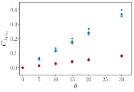
$(a)$                                                    $(b)$
      
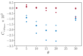
$(c)$                                                    $(d)$

Figure 17: Contributions to $C_{\perp}(\raisebox{1.5pt}{$\chi$},\theta,\text{Re})$ at $\text{Re}=20$ (blue) and $\text{Re}=300$ (red) for $\bullet$: $\raisebox{1.5pt}{$\chi$}=3$, $\star$: $\raisebox{1.5pt}{$\chi$}=5$, +: $\raisebox{1.5pt}{$\chi$}=7$. $(a)$ pressure on the lateral surface; $(b)$ viscous stress on the lateral surface; $(c),\,(d)$ viscous stress on the upstream and downstream ends, respectively.

where $U_{\perp}=||\bf{U}||\sin\theta$ is the component of the upstream velocity normal to the lateral surface and the Reynolds number Re is based on the norm of the upstream velocity. In this Reynolds number range, $C_{\perp}^{\theta=90^{\circ}}$ is almost constant according to (19), so that (21) indicates that the perpendicular force is approximately proportional to the power three-half of the incoming velocity, while it still varies almost linearly with $\theta$. In contrast, the Independence Principle frequently invoked in the area of vortex-induced vibrations [10, 15] suggests that the perpendicular force on a long cylinder should only depend on the normal component $U_{\perp}$ of the incoming flow, which would imply $F_{\perp}=\frac{1}{2}C_{\perp}^{\theta=90^{\circ}}(\raisebox{1.5pt}{$\chi$}\gg 1,Re_{\perp})\rho LD||{\bf{U}}_{\perp}||U_{\perp}$, with $\text{Re}_{\perp}=\rho||{\bf{U}}_{\perp}||D/\mu$. If this were true in the present situation, a $\sin^{2}\theta$-dependence of $C_{\perp}$ would be observed for $\text{Re}_{\perp}=\mathcal{O}(10^{2})$ (i.e. $\text{Re}=300$ here in practice), and the force would vary as the square of the incoming velocity. As Fig. 16$(f)$ indicates, no quadratic dependence with respect to the inclination angle is noticed, which implies that the Independence Principle does not apply to the flow configurations under consideration. This is in line with the conclusions of [12] where it was observed at somewhat lower Reynolds numbers that this ‘principle’ only holds for inclinations larger than $70^{\circ}$ but overestimates the force by more than $50\%$ for $\theta\leq 30^{\circ}$, even for long cylinders with $\raisebox{1.5pt}{$\chi$}=15$. In other words, this ‘principle’ is approximately valid when the upstream flow is almost normal to the cylinder lateral surface but can by no means be used to approximate the transverse force when the cylinder inclination is moderate.

V.3 Approximate laws for the parallel force and spanwise torque

Figure 18 shows the main contributions to $C_{\parallel}(\raisebox{1.5pt}{$\chi$},\theta,\text{Re})$ arising from pressure and viscous stress distributions over the various parts of the cylinder surface. On both ends, the latter (not shown) are found to be more than one order of magnitude smaller than the former. Therefore, $C_{\parallel}$ is essentially controlled by the viscous stress acting on the lateral surface and the pressure distribution on both ends. All contributions are seen to decrease for increasing aspect ratios, similar to what happens when the body is aligned with the incoming flow. This influence weakens significantly as Re increases, again in line with the observations reported for $\theta=0^{\circ}$. In particular, the viscous contribution arising from the lateral surface (Fig. 18$(c)$) is found to be virtually independent of $\chi$ for $\text{Re}=300$. That these features subsist for all inclinations considered here suggests that seeking an empirical expression relating $C_{\parallel}(\raisebox{1.5pt}{$\chi$},\theta,\text{Re})$ to $C_{\parallel\theta=0^{\circ}}(\raisebox{1.5pt}{$\chi$},\text{Re})$ is reasonable. Variations with $\theta$ follow different and sometimes opposite trends on the various surfaces. For instance, Fig. 18$(a)$ indicates that $C_{\parallel p_{up}}$ decreases as the inclination increases, an effect weakening at large Reynolds number.

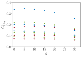
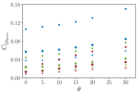
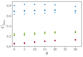
$(a)$                                         $(b)$                                          $(c)$

Figure 18: Contributions to $C_{\parallel}(\raisebox{1.5pt}{$\chi$},\theta,\text{Re})$ at $\text{Re}=20$ (blue), $\text{Re}=80$ (green) and $\text{Re}=300$ (red) for $\bullet$: $\raisebox{1.5pt}{$\chi$}=3$, $\star$: $\raisebox{1.5pt}{$\chi$}=5$, +: $\raisebox{1.5pt}{$\chi$}=7$. $(a)-(b)$ pressure on the upstream and downstream ends, respectively; $(c)$ viscous stress on the lateral surface.

In contrast, $C_{\parallel p_{down}}$ (Fig. 18$(b)$) increases gradually with $\theta$. This is because the recirculating region at the back of the cylinder tends to shrink when $\theta$ increases, as noticed in Sec. V.1. A significant increase of $C_{\parallel\mu_{lat}}$ is also noticed at $\text{Re}=300$ (Fig. 18$(c)$), but this trend weakens as Re decreases and is no longer present at $\text{Re}=20$.
To approximate the variations of $C_{\parallel}$ with $\raisebox{1.5pt}{$\chi$},\,\theta$ and Re, we started from the fits (6)-(8) established for $\theta=0^{\circ}$ in Sec. III.2. We took into account the constraint that $C_{\parallel}$ cannot depend on the sign of $\theta$ and must change sign for $\theta=90^{\circ}$, although this configuration is well beyond the maximum inclination considered in the simulations. This led us to assume that the leading-order angular dependence of the correction to the ‘Stokes law’ is proportional to $\sin^{2}\theta\cos\theta$. Then, we first considered the case $\raisebox{1.5pt}{$\chi$}=7$ for which finite-length effects are the weakest, and started to fit the dependence with respect to Re for $\theta=30^{\circ}$, the maximum inclination. The behavior of $C_{\parallel}$ at median inclinations suggests that the angular dependence also involves a secondary contribution that may be approached by a term proportional to $\sin^{2}6\theta\cos\theta$. Last, we considered finite-length effects, starting with $\raisebox{1.5pt}{$\chi$}=3$ for which they are most severe. All empirical pre-factors were constrained to vanish for $\text{Re}\rightarrow 0$, so that $C_{\parallel}$ reduces to its low-Re form in this limit. The whole process was carried out iteratively, to optimize the pre-factors and exponents for the three aspect ratios over the whole range of Re and $\theta$. Keeping in mind that the drag coefficient $C_{d}(\raisebox{1.5pt}{$\chi$},Re)$ determined in Sec. III.2 by summing (6)-(8) has to be multiplied by a factor $\frac{\pi}{4}\raisebox{1.5pt}{$\chi$}^{-1}$ to be used in the prediction of $C_{\parallel}$, the final fit takes the form

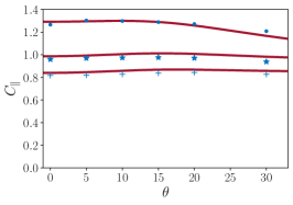
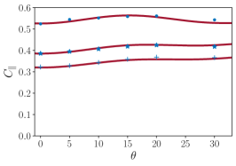
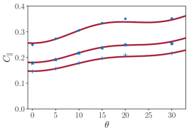
$(a)$                                           $(b)$                                           $(c)$
$\text{Re}=20$                                     $\text{Re}=80$                                     $\text{Re}=300$

Figure 19: Parallel force coefficient $C_{\parallel}(\raisebox{1.5pt}{$\chi$},\theta,\text{Re})$ vs. $\theta$ for $\bullet$: $\raisebox{1.5pt}{$\chi$}=3$, $\star$: $\raisebox{1.5pt}{$\chi$}=5$, +: $\raisebox{1.5pt}{$\chi$}=7$. Solid line: empirical fit (22).

$$C_{\parallel}(\raisebox{1.5pt}{$\chi$},\theta,\text{Re})\approx\frac{\pi}{4}\raisebox{1.5pt}{$\chi$}^{-1}C_{d}(\raisebox{1.5pt}{$\chi$},Re)\biggl{\{}1+\left[(0.7-6.3\raisebox{1.5pt}{$\chi$}^{-2})(1-e^{-0.15\text{Re}})+0.01\text{Re}^{0.95}\right]\sin^{2}\theta+2\times 10^{-3}\text{Re}^{0.8}\sin^{2}6\theta\biggr{\}}\cos\theta\,.$$ (22)

As Fig. 19 shows, this fit provides a correct estimate of $C_{\parallel}$ throughout the range of parameters explored in the present investigation. Expression (22) highlights the fact that inertial effects act to increase $C_{\parallel}$ and counteract the $\cos\theta$-decrease associated with viscous effects, and even overtake them for high enough Re (for large $\chi$ and $\text{Re}\gtrsim 10$, the dominant contribution to the term within curly brackets is $1+\left(0.7+0.01\text{Re}^{0.95}\right)\sin^{2}\theta$). Obviously, the above fit is not expected to be valid for Reynolds numbers significantly larger than the upper bound considered in the simulations, as it predicts a diverging drag in the limit $\text{Re}\rightarrow\infty$. Similarly, (22) is not expected to hold for larger inclinations: in [13] it was observed that, for $\raisebox{1.5pt}{$\chi$}=3$ and $\text{Re}=250$, $C_{\parallel}$ sharply decreases in the range $30^{\circ}<\theta<45^{\circ}$, a trend that the above fit is clearly unable to reproduce.

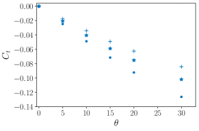
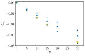
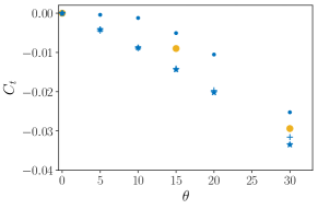
$(a)$                                               $(b)$                                               $(c)$
$\text{Re}=20$                                         $\text{Re}=80$                                         $\text{Re}=300$

Figure 20: Torque coefficient vs. $\theta$ for $\bullet$: $\raisebox{1.5pt}{$\chi$}=3$, $\star$: $\raisebox{1.5pt}{$\chi$}=5$, + $\raisebox{1.5pt}{$\chi$}=7$. The yellow bullets in panels $(b)$ and $(c)$ refer to the results of [13] for $\raisebox{1.5pt}{$\chi$}=3$ at $\text{Re}=75$ and $250$, respectively.

Figure 20 shows the variations of the torque coefficient as a function of $\theta$. Similar to the low-to-moderate Re regime, the torque is always negative, tending to orient the cylinder axis perpendicular to the upstream flow. The torque coefficient exhibits a quasilinear increase with the inclination angle for $\raisebox{1.5pt}{$\chi$}=5$ and $7$. This may be seen as a natural extension of the $\sin 2\theta$-variation characterizing the $C_{t}$-variations at low Re. $|C_{t}|$ is also found to decrease for increasing $\chi$ at $\text{Re}=20$ and $\text{Re}=80$. The behavior observed at $\text{Re}=300$ is more complex, especially in the case of the shortest cylinder for which the angular dependence is strongly nonlinear for $\theta\lesssim 15^{\circ}$. Moreover, while the corresponding $|C_{t}|$ is larger than those of the other two cylinders at $\text{Re}=20$ and $\text{Re}=80$, the situation is reversed at $\text{Re}=300$. Some additional insight into these variations may again be obtained by splitting the torque into pressure and viscous contributions provided by each part of the cylinder surface. The main contributions resulting from this decomposition are displayed in Fig. 21. The two dominant terms are seen to result from the pressure distribution on the lateral surface ($C_{{tp}_{lat}}$) and the viscous stress on the upstream end ($C_{{t\mu}_{up}}$). Both terms decrease in magnitude with increasing $\chi$ and Re, keeping a negative sign in all cases. The third and fourth contributors, $C_{{tp}_{up}}$ and $C_{{t\mu}_{lat}}$, result from the pressure and viscous stress distributions on the same surfaces. The contributions of the downstream end (not shown) are one order of magnitude smaller than the dominant terms in all cases. In contrast to its viscous counterpart ($C_{{t\mu}_{up}}$), $C_{{tp}_{up}}$ is seen to keep a positive sign in all cases. The three contributions $C_{{tp}_{lat}}$, $C_{{tp}_{up}}$ and $C_{{t\mu}_{up}}$ vary almost linearly with $\theta$ whatever $\chi$ and Re. The viscous contribution associated with the lateral surface, $C_{{t\mu}_{lat}}$ (Fig. 21$(d)$), reveals a more complex behavior. First, its sign changes with $\chi$ and Re. It stays positive whatever $\theta$ for the shortest cylinder, increasing in magnitude as Re increases. Conversely, it is negative for the longest two cylinders at $\text{Re}=20$, gradually decreasing until changing sign at all inclinations for $\text{Re}=300$. Second, variations of $C_{{t\mu}_{lat}}$ with $\theta$ become increasingly nonlinear as $\chi$ decreases and/or Re increases. This complex behavior is responsible for the markedly nonlinear variations of $C_{t}$ with $\theta$ noticed above for the shortest cylinder at $\text{Re}=300$. The open separation process discussed in Sec. V.1 is responsible for these features. Indeed, the dominant local viscous contribution to the spanwise torque provided by the the lateral surface is, in dimensional form, $-\mu\frac{D}{2}\frac{{\bf{r}}\cdot{\bf{e_{y}}}}{||{\bf{r}}||}({\bf{n}}\cdot\nabla)u_{\parallel}$, where $u_{\parallel}$ is the fluid velocity component parallel to this surface (along the $x$-direction), ${\bf{n}}$ is the unit normal directed into the fluid and ${\bf{r}}$ is the local position with respect to the cylinder geometrical center. As far as the fluid does not recirculate, this term is positive on the lower part of the surface (${\bf{r}}\cdot{\bf{e_{y}}}<0$) and negative on the upper part (${\bf{r}}\cdot{\bf{e_{y}}}>0$). However, when separation takes place, $u_{\parallel}$ is negative in the corresponding region of the upper part, which then provides a positive viscous contribution, making $C_{{t\mu}_{lat}}$ positive if the recirculation is strong enough. The larger the area percentage of the lateral surface corresponding to the separated region, the larger the positive value of $C_{{t\mu}_{lat}}$.

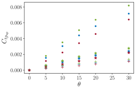
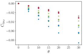
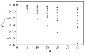
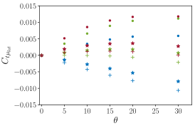
$(a)$                                               $(b)$
$(c)$                                               $(d)$

Figure 21: Contributions to $C_{t}(\raisebox{1.5pt}{$\chi$},\theta,\text{Re})$ at $\text{Re}=20$ (blue), $\text{Re}=80$ (green) and $\text{Re}=300$ (red) for $\bullet$: $\raisebox{1.5pt}{$\chi$}=3$, $\star$: $\raisebox{1.5pt}{$\chi$}=5$, +: $\raisebox{1.5pt}{$\chi$}=7$. $(a)-(b)$ pressure on the upstream end and the lateral surface, respectively; $(c)-(d)$ viscous stress on the upstream end and the lateral surface, respectively.

Following a fitting procedure similar to that described for $C_{\parallel}$, we approached the behaviors observed in Fig. 20 with the empirical expression

$$C_{t}(\raisebox{1.5pt}{$\chi$},\theta,\text{Re})\approx\raisebox{1.5pt}{$\chi$}^{-0.47}\left\{-0.69\text{Re}^{-0.35-b_{1}(\text{Re}/\raisebox{1.5pt}{$\chi$})^{3.1}}\sin 2\theta+1\times 10^{-4}\text{Re}^{0.8+b_{2}(\text{Re}/\raisebox{1.5pt}{$\chi$})^{3.1}}\sin 6\theta\right\}\,,$$ (23)

with $b_{1}=7\times 10^{-8}$ and $b_{2}=5\times 10^{-8}$.

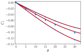
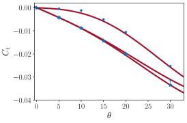
$(a)$                                             $(b)$                                             $(c)$
$\text{Re}=20$                                       $\text{Re}=80$                                      $\text{Re}=300$

Figure 22: Torque coefficient $C_{t}(\raisebox{1.5pt}{$\chi$},\theta,\text{Re})$ vs. $\theta$ for $\bullet$: $\raisebox{1.5pt}{$\chi$}=3$, $\star$: $\raisebox{1.5pt}{$\chi$}=5$, +: $\raisebox{1.5pt}{$\chi$}=7$. Solid line: empirical fit (23).

As Fig. 22 shows, the above fit provides a correct estimate of $C_{t}$ throughout the range of parameters explored in the present investigation. For large enough aspect ratios, the dominant contribution to $C_{t}$ is still proportional to $\sin 2\theta$, similar to the low-Re-regime, and its magnitude varies as $\raisebox{1.5pt}{$\chi$}^{-0.47}Re^{-0.35}$. The torque coefficient is seen to be approximately proportional to $\raisebox{1.5pt}{$\chi$}^{-1/2}$ whatever Re, which suggests that the dimensional torque behaves roughly like $L^{3/2}$ for long enough cylinders. Finite-length high-Re effects associated with the open separation are translated into the above fit through the slight but sharp $(\text{Re}/\raisebox{1.5pt}{$\chi$})^{3.1}$-increase of the Reynolds number exponent. Similar to the case of $C_{\parallel}$, the above fit is not expected to be valid for Reynolds numbers significantly larger than the upper bound considered in the simulations. Moreover, although (23) respects the constraint that the torque changes sign for $\theta=90^{\circ}$, the results of [13] for a cylinder with $\raisebox{1.5pt}{$\chi$}=3$ indicate that the behavior of $C_{t}$ changes significantly for $\theta\gtrsim 45^{\circ}$, suggesting that the present fit is appropriate only below this critical inclination.

VI Summary and concluding remarks

With the practical objective of providing approximate laws for predicting the translation-induced drag, lift and torque acting on long cylindrical rods and fibers, we employed fully-resolved simulations to investigate the flow around a finite-length circular cylinder held fixed in a uniform stream making some angle with the body axis.
We first focused on the specific case where the cylinder is aligned with the incoming flow. Considering the Stokes regime and the weakly inertial regime corresponding to $\text{Re}\lesssim 1$, we combined numerical results with available predictions from the slender-body theory (which we slightly improved by computing the next-order term in the expansion with respect to the small parameter $1/\ln(2\raisebox{1.5pt}{$\chi$})$) to build the approximate drag laws (1) and (5). The former is valid down to $\raisebox{1.5pt}{$\chi$}\approx 1.5$, while the inertial corrections contained in the latter allow an accurate estimate of the drag up to $\text{Re}=\mathcal{O}(1)$, and even up to $\text{Re}=\mathcal{O}(10)$ for $\raisebox{1.5pt}{$\chi$}\gtrsim 20$. For larger Reynolds numbers (up to $\text{Re}=400$), the flow structure becomes more complex, although it remains stationary and axisymmetric. Beyond a $\chi$-dependent critical Reynolds number of the order of $200$, a second recirculating region emerges along the upstream part of the lateral surface. Being associated with local negative shear stresses, this lateral eddy acts to reduce the friction drag, which may even become negative if Re is large enough and the cylinder is short enough. We used the numerical data to build approximate fits for this friction drag and for the pressure drag contribution of the upstream and downstream ends. With this procedure, we obtained the empirical drag law (9) which approximates the drag well for $\raisebox{1.5pt}{$\chi$}\gtrsim 2$ in the range $20\leq\text{Re}\leq 400$ and properly matches (5) for $\text{Re}=\mathcal{O}(1)$. The friction drag still represents a substantial part of the total drag at Reynolds numbers of several hundreds if the body aspect ratio is large enough ($45\%$ at $\text{Re}=400$ for a cylinder with $\raisebox{1.5pt}{$\chi$}=10$).
In the next step, we examined the case of moderately inclined cylinders ($\theta\leq 30^{\circ}$) in the low-to-moderate Reynolds number regime ($\text{Re}\leq 5$). For Reynolds numbers less than unity and aspect ratios up to $10$, we observed that the force component parallel to the cylinder axis closely follows the $\cos\theta$-variation predicted under creeping-flow conditions. The agreement deteriorates as the length-based Reynolds number $\chi$Re exceeds values of $\mathcal{O}(10)$. Under more inertial conditions, the $\cos\theta$-law under-predicts the actual parallel force, the difference increasing with both $\chi$Re and $\theta$. The force component perpendicular to the cylinder axis was found to closely follow the $\sin\theta$-variation typical of creeping-flow conditions up to $\text{Re}=5$, irrespective of $\chi$. However, the corresponding pre-factor deviates from the creeping-flow prediction as soon as $\raisebox{1.5pt}{$\chi$}\text{Re}\gtrsim 0.5$, beyond which inertial effects become significant. Accurate predictions are obtained up to $\raisebox{1.5pt}{$\chi$}\text{Re}\approx 10$ by estimating the pre-factor of the $\sin\theta$-law through the semi-empirical formula (34) which provides a finite-Reynolds-number approximation of $F_{\perp}^{\theta=90^{\circ}}$. Throughout the low-to-moderate Reynolds number range, the inertial torque follows the $\sin 2\theta$-variation predicted by the asymptotic theory of Khayat and Cox [4] in the limit $\raisebox{1.5pt}{$\chi$}\text{Re}\ll 1$. However the magnitude of the torque is correctly predicted by this theory only up to $\text{Re}=\mathcal{O}(1)$ and provided $\text{Re}/\raisebox{1.5pt}{$\chi$}^{2}\lesssim 0.01$. To obtain a correct estimate of the torque over a broader range of conditions, we derived the semiempirical law (18) which correctly reduces to the theoretical prediction in the limit $\raisebox{1.5pt}{$\chi$}\text{Re}\ll 1,\raisebox{1.5pt}{$\chi$}\gg 1$ and closely approaches numerical data for cylinders with $\raisebox{1.5pt}{$\chi$}\geq 5$ up to $\text{Re}=5$.
Last we considered the three-dimensional flow past moderately inclined cylinders with aspect ratios in the range $3-7$ for $20\leq\text{Re}\leq 300$. For $\theta\leq 30^{\circ}$, the flow remains stationary irrespective of the inclination and preserves a symmetry with respect to the plane containing the body axis and the incoming velocity. For sufficiently low inclinations and Reynolds numbers, the flow separates only at the back of the body, the recirculating region looking like an open toroid. In contrast, beyond a critical inclination decreasing as Re increases, an open separated region emerges on the ‘extrados’ of the lateral surface, near its ‘leading edge’. In such configurations, the flow past the cylinder looks massively separated in between the two free streamlines emanating from its ‘trailing’ and ‘leading’ edges.
We used numerical data collected in this fully inertial regime to obtain approximate laws for the loads acting on the cylinder. Similar to the the low-Re behavior, the perpendicular force obeys essentially a $\sin\theta$-variation with a mild dependence with respect to the aspect ratio. We found that the corresponding force coefficient $C_{\perp}$ may be related to the drag coefficient of a cylinder held perpendicular to the incoming flow through the emprical law (20) which involves two simple independent corrections, one proportional to $\text{Re}^{-1/2}$ accounting for inertial effects, the other for finite-length effects.

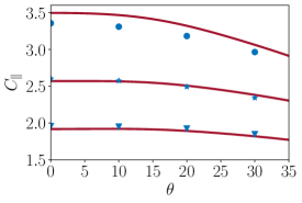
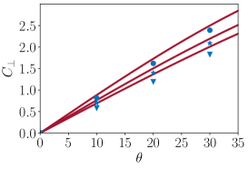
$(a)$                                             $(b)$                                               $(c)$

Figure 23: Extrapolated predictions at $\text{Re}=5$ of fits derived in the fully inertial regime for $\bullet$: $\raisebox{1.5pt}{$\chi$}=3$, $\star$: $\raisebox{1.5pt}{$\chi$}=5$, +: $\raisebox{1.5pt}{$\chi$}=7$. $(a)$ $C_{\parallel}$ and fit (22); $(b)$ $C_{\perp}$ and fit (20); $(c)$ $C_{t}$ and fit (23).

In contrast, variations of the parallel force do not follow the $\cos\theta$-law prevailing in the low-Re regime. Instead, the force coefficient $C_{\parallel}$ barely varies with $\theta$ in the moderate-Re regime and even increases with the inclination at large Reynolds number. A fitting procedure with respect to the three control parameters allowed us to mimic the influence of inertial and finite-length effects on $C_{\parallel}$ through the empirical law (22) which reproduces all observed trends well. Variations of the spanwise torque at moderate Reynolds number are qualitatively similar to those observed for $\text{Re}\leq 5$. However strong finite-length effects manifest themselves at high Reynolds number, in connection with the separation process affecting the upstream part of the lateral surface in this regime. A fitting approach similar to that employed for $C_{\parallel}$ yielded the empirical law (23) which correctly approximates $C_{t}$ throughout the explored range of $\chi$ and $\theta$ in the fully inertial regime. For application purposes, it is of course of interest to know how robust these fits determined from data in the range $20\leq\text{Re}\leq 300$ are when the Reynolds number is decreased to the upper limit of the low-to-moderate Re regime considered in Sec. IV. The results or this test are summarized in Fig. 23. It turns out that the empirical formula established in the fully inertial regime still perform quite well for $\text{Re}=5$. Predictions depart from numerical data by less than $5\%$ for $C_{\parallel}$, $10\%$ for $C_{\perp}$ and $15\%$ for $C_{t}$. Therefore, the semi-empirical predictions derived in Sec. IV combined with the fits established in Sec. V offer a complete and almost smooth description of load variations from the creeping-flow regime up to $\text{Re}=300$.
Most computations only considered aspect ratios below $10$ or even $7$ for $\text{Re}\geq 20$, owing to the rapid increase of computational costs with $\chi$. However, finite-length effects were found to decrease monotonically and sharply as $\chi$ increases, making us confident that the various empirical laws derived in the course of this study remain valid for cylindrical particles with larger aspect ratios, and therefore apply to long fibers. Obviously this does not mean that the load coefficients become independent of $\chi$ for $\raisebox{1.5pt}{$\chi$}\gg 1$, but simply that their asymptotic dependence with respect to $\chi$ in the limit of large aspect ratios is already captured by considering $\mathcal{O}(10)$-aspect ratios as we did. The situation is less clear regarding their range of validity with respect to the inclination angle. All of them were calibrated in the range $|\theta|\leq 30^{\circ}$ and satisfy the required geometrical constraints for $|\theta|=90^{\circ}$ and the associated symmetry conditions. Nevertheless, as soon as the Reynolds number exceeds a few tens, the dynamics of the flow past a cylinder in the configuration $\theta=90^{\circ}$ drastically differs from that past the same cylinder for $\theta=0^{\circ}$. Hence, physical features that are not present in the low-to-moderate inclination range considered here take place in the near-body flow when the inclination exceeds $45^{\circ}$ or so, which is likely to make the empirical laws proposed here invalid for such large inclinations.
The present investigation leaves several important configurations and parameter ranges unexplored. First, for Reynolds numbers similar to those considered in Secs. IV and V, the above discussion calls for a specific study focused on large inclinations, say $45^{\circ}\lesssim|\theta|\leq 90^{\circ}$, for which the flow past the cylinder is expected to be massively separated and most of the time unsteady. Another series of questions arises when the cylinder is allowed to rotate about an axis perpendicular to its symmetry axis and passing through its geometrical center, as rodlike particles and fibers customarily do. The torque on a slender rotating cylinder was predicted in the creeping flow limit in [1, 2] but no theoretical attempt to derive inertial corrections in this configuration has been reported so far. This is even more true for the general situation in which the cylinder undergoes both a translation and a rotation. In such a case, inertial effects couple the two types of motion, yielding specific contributions to the loads, which are for instance responsible for the well-known Magnus effect on a spinning sphere. To the best of our knowledge, such couplings have not been considered for slender cylinders. We are currently investigating numerically the configuration in which the cylinder undergoes an imposed rotation, and plan to apply the same methodology to the combined translation+rotation case in the near future.

Appendix A Specific numerical validations

As mentioned in Sec. II, the JADIM code was extensively used in the past to compute flows past axisymmetric bodies. In particular, transitional flows past disks and short cylinders were considered in [18, 19, 20]. Nevertheless, we performed additional validations relevant to the present physical configuration by considering the flow past an inclined cylinder of aspect ratio $\raisebox{1.5pt}{$\chi$}=3$ for different Reynolds numbers and inclination angles.

	Number of cells across the boundary layer	$C_{d}$	Error %
$\text{Re}=100,\theta=5^{\circ}$	5	0.478	0.62
	8	0.479	0.4
	10	0.481	-
$\text{Re}=100,\theta=15^{\circ}$	5	0.546	2.2
	8	0.534	0.37
	10	0.532	-
$\text{Re}=200,\theta=15^{\circ}$	5	0.416	1.4
	8	0.411	0.2
	10	0.410	-

Table 1: Drag coefficient obtained with three different grids (with 5, 8 and 10 cells across the boundary layer, respectively), and three different flow configurations. The relative error is based on the most refined grid.

We first performed runs with an increasing number of cells across the boundary layer, the thickness of which is estimated as $D\text{Re}^{-1/2}$. Table 1 shows the effect of the grid refinement on the drag coefficient (here defined as the drag force normalized by${LD\rho U^{2}}/2$) for three different configurations. Clearly, eight cells across the boundary layer suffice to properly capture viscous effects, since the relative difference with the drag obtained on the most refined grid is less than 1% in each configuration.

Re	$\theta$	$C_{d}$		$E(C_{d})\%$
		[13]	Present results
100	$5^{\circ}$	0.472	0.479	1.4
	$10^{\circ}$	0.499	0.501	0.4
	$15^{\circ}$	0.536	0.534	0.3
	$30^{\circ}$	0.693	0.680	1.4
200	$10^{\circ}$	0.350	0.345	$1.4$
	$15^{\circ}$	0.405	0.411	1.5

Table 2: Comparison of the drag coefficient obtained with the present numerical methodology with results of [13] for $5^{\circ}\leq\theta\leq 30^{\circ}$ and two moderate Reynolds numbers. $E(C_{d})$ is the relative difference between the drag coefficients provided by the two sources.

Then we checked present results obtained with eight cells across the boundary layer against those of [13] based on the PELIGRIFF code [37]. Table 2 shows how the two sets of the results compare for six different flow configurations. The drag coefficients are seen to differ by less than $1.5\%$ in all cases.

Appendix B Higher-order zero-Reynolds-number slender-body prediction for the drag on a finite-length cylinder aligned with the flow or perpendicular to it

The hydrodynamic force experienced by a slender body immersed in a nonuniform flow was derived independently by Batchelor [1], Cox [2] and Keller and Rubinow [25] in the form of an expansion with respect to the small parameter $1/\ln(2\raisebox{1.5pt}{$\chi$})$ for $\raisebox{1.5pt}{$\chi$}\gg 1$. References [1] and [25] provide an expansion up to order 3 in this small parameter. However, the logarithmic dependence of the force with respect to $\chi$ makes higher-order contributions significant as soon as $\chi$ becomes of $\mathcal{O}(10)$ or less. This is why a higher-order prediction is desirable to obtain a more accurate evaluation of the force on moderately-long cylinders. In this appendix, restricting ourselves to the case where the cylinder is aligned with the incoming flow, we provide the expression for the drag valid up to order 4, based on the expansion carried out in [25].
The total force experienced by a slender fiber of length $L$ immersed in a viscous flow may be expressed in the form

$$\mathbf{F}=-8\pi\mu L\int_{0}^{1}\mathbf{f}(s)\mathrm{d}s\,,$$ (24)

where $\mathbf{f}(s)$ is the density of the Stokeslet distribution along the body centerline and $s$ denotes the arc length. The density $\mathbf{f}$ is obtained through a matched asymptotic procedure, the details of which may be found in [25]. If the body is a circular cylinder aligned with the flow direction, one has $\mathbf{f}(s)=f_{x}(x)\mathbf{e_{x}}$ with

$$f_{x}(x)=-\frac{1}{2\ln\left(2\raisebox{1.5pt}{$\chi$}\right)}\left(\frac{U_{x}}{2}+f_{x}(x)\left(\ln(4x(1-x))-1\right)+\int_{-x}^{1-x}\frac{f_{x}(x+t)-f_{x}(x)}{|t|}dt\right)\,,$$ (25)

where $U_{x}=\bf{U}\cdot\bf{e_{x}}$. An approximate solution of (25) may be obtained by successive approximations. Setting $f_{x}=0$ in the right-hand side, the first-order approximation is found to be $f_{x}^{(1)}=-U_{x}/(4\ln\left(2\raisebox{1.5pt}{$\chi$})\right)$. The iterative solution was obtained in [25] up to order 3 in the form

$$f_{x}^{(3)}(x)=-\frac{U_{x}}{4\ln\left(2\raisebox{1.5pt}{$\chi$}\right)} \left(1-\frac{1}{2\ln\left(2\raisebox{1.5pt}{$\chi$}\right)}\left(\ln(4x(1-x))-1\right)+\frac{1}{(2\ln\left(2\raisebox{1.5pt}{$\chi$}\right))^{2}}\left(\ln(4x(1-x))-1\right)^{2}\right.$$

$$\left.+\frac{1}{(2\ln\left(2\raisebox{1.5pt}{$\chi$}\right))^{2}}\int_{-x}^{1-x}\frac{\ln((x+t)(1-x-t))-\ln(x(1-x))}{|t|}dt\right).$$ (26)

Integrating the penultimate term in (26), we obtain

$$F_{x}^{(3)}= -8\pi\mu L\int_{0}^{1}f_{x}^{(3)}(x)\mathrm{d}x=2\pi\mu LU_{x}\left(\frac{a_{x}^{(1)}}{\ln(2\raisebox{1.5pt}{$\chi$})}+\frac{a_{x}^{(2)}}{(\ln(2\raisebox{1.5pt}{$\chi$}))^{2}}+\frac{a_{x}^{(3)}}{(\ln(2\raisebox{1.5pt}{$\chi$}))^{3}}\right)\,,$$ (27)

with $a_{x}^{(1)}=1$, $a_{x}^{(2)}=3/2-\ln 2\approx 0.80685$, and $a_{x}^{(3)}=13/4-\pi^{2}/12+\ln 2(\ln 2-3)\approx 0.82854$. This result agrees with those of [1] and [25]. At next order, the force density may be obtained by inserting (26) in the right-hand side of (25), yielding

$$f_{x}^{(4)}(x) =-\frac{U_{x}}{4\ln\left(2\raisebox{1.5pt}{$\chi$}\right)}\left(1-\frac{1}{2\ln\left(2\raisebox{1.5pt}{$\chi$}\right)}\left(\ln(4x(1-x))-1\right)+\frac{1}{(2\ln\left(2\raisebox{1.5pt}{$\chi$}\right))^{2}}\left(\ln(4x(1-x))-1\right)^{2}\right.$$

$$\left.-\frac{1}{(2\ln\left(2\raisebox{1.5pt}{$\chi$}\right))^{3}}\left[\left(\ln(4x(1-x))-1\right)^{3}+\left(\ln(4x(1-x))-1\right)\int_{-x}^{1-x}\frac{\ln((x+t)(1-x-t))-\ln(x(1-x))}{|t|}dt\right]\right.$$

$$\left.-\frac{1}{(2\ln\left(2\raisebox{1.5pt}{$\chi$}\right))^{3}}\int_{-x}^{1-x}\frac{f_{x}^{(3)}(x+t)-f_{x}^{(3)}(x)}{|t|}dt\right).$$ (28)

The drag acting on the body is eventually obtained by making use of the previous expression in (24) and integrating along the body centerline. Since the last term in (28) does not contribute to the force [25], one is left with

$$F_{x}^{(4)}=F_{x}^{(3)}+2\pi\mu LU_{x}\left(\frac{a_{x}^{(4)}}{(\ln(2\raisebox{1.5pt}{$\chi$}))^{4}}\right)\,,$$ (29)

with $a_{x}^{(4)}=\left[-10\zeta(3)+79+\pi^{2}(\ln 4-3)-\ln 4(39+(\ln 4)^{2}-9\ln 4)\right]/8\approx 1.45243$, $\zeta$ denoting the Riemann zeta function. The main difficulty in the integration required to obtain $a^{(4)}$ results from the first integral in the right-hand side of (28). A formal computation using Mathematica^TM indicates that this term provides a contribution of $2\zeta(3)$.

Appendix C Drag force on a cylinder held perpendicular to the flow: Slender-body approximation and semiempirical laws at zero and low-but-finite Reynolds number

Due to the linearity of the Stokes equation, the force acting on an arbitrarily inclined cylinder in the low-Re regime may be obtained by suitably combining linearly the drag forces corresponding to the aligned ($\theta=0^{\circ}$) and perpendicular ($\theta=90^{\circ}$) configurations. This is why an accurate estimate of the zero-Re drag force on a finite-length cylinder held perpendicular to the incoming flow is desirable. To our surprise, such an estimate does not seem to be available in the literature. Clift et al. [24] proposed an empirical relationship accurate for moderate aspect ratios but did not match it with the prediction of the the slender-body theory in the limit of large aspect ratios. In this appendix, we first use the methodology employed in appendix B to establish the $4^{th}$-order slender-body approximation of the corresponding drag force at $\text{Re}=0$. Then we modify the corresponding expression in an ad hoc manner to extend its validity to short cylinders, before incorporating the finite-$Re$ correction derived in [4].
Duplicating the technique used in appendix B, the density of the Stokeslet distribution $f_{y}$ required to obtain the force $F_{y}$ on the cylinder is obtained by replacing $\ln(4x(1-x))-1$ everywhere with $\ln(4x(1-x))+1$, and $U_{x}$ with $2U_{y}$ in (28) [25]. Then the total force is found to be

$$F_{y}^{(4)}= -8\pi\mu L\int_{0}^{1}f_{y}^{(4)}(x)\mathrm{d}x=4\pi\mu LU_{y}\left(\frac{a_{y}^{(1)}}{\ln(2\raisebox{1.5pt}{$\chi$})}+\frac{a_{y}^{(2)}}{(\ln(2\raisebox{1.5pt}{$\chi$}))^{2}}+\frac{a_{y}^{(3)}}{(\ln(2\raisebox{1.5pt}{$\chi$}))^{3}}+\frac{a_{y}^{(4)}}{(\ln(2\raisebox{1.5pt}{$\chi$}))^{4}}\right)\,,$$ (30)

with $a_{y}^{(1)}=1$, $a_{y}^{(2)}=1/2-\ln 2\approx-0.19315$, $a_{y}^{(3)}=5/4-\pi^{2}/12+\ln 2(\ln 2-1)\approx 0.21484$ and $a_{y}^{(4)}=\left[-10\zeta(3)+29+\pi^{2}(\ln 4-1)-\ln 4(15+(\ln 4)^{2}-3\ln 4)\right]/8\approx 0.38735$.

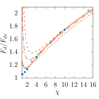
Figure 24: Drag on a finite-length cylinder held perpendicular to the flow direction, normalized by the drag $F_{ds}$ of a sphere of same volume. Dotted, dash-dotted and dashed lines: slender-body approximation (30) truncated at $2^{nd}$, $3^{rd}$ and $4^{th}$ order, respectively; solid line: semiempirical formula (31); $\bullet$: numerical results of [38]; $\blacksquare$: experimental results of [27]; $\blacktriangledown$: experimental results of [39].

Figure 24 displays the corresponding successive predictions and compares them with experimental and numerical data. The $3^{rd}$-order approximation provides a fairly good agreement for small-to-moderate aspect ratios. However, neither the $2^{nd}$-order nor the $3^{rd}$-order approximation properly matches available data in the limit of high aspect ratios. The $4^{th}$-order approximation provides a better prediction at high $\chi$ but quickly diverges as $\chi$ becomes less than $\approx 4$. Based on these observations, we empirically modify (30) by weighting the third- and fourth-order terms with a pre-factor that quickly varies from $1$ for moderate-to-large $\chi$ to $0$ for $\chi\rightarrow 1/2$, in such a way that the behavior of the $3^{rd}$-order expansion is recovered for moderate aspect ratios. The corresponding modified drag law reads

$$F_{y}^{(4)}=-8\pi\mu L\int_{0}^{1}f_{y}^{(4)}(x)\mathrm{d}x=4\pi\mu LU_{y}\left(\frac{a_{y}^{(1)}}{\ln(2\raisebox{1.5pt}{$\chi$})}+\frac{a_{y}^{(2)}}{(\ln(2\raisebox{1.5pt}{$\chi$}))^{2}}+\left(1-e^{-c_{1}\raisebox{1.5pt}{$\chi$}^{c_{2}}}\right)\left(\frac{a_{y}^{(3)}}{(\ln(2\raisebox{1.5pt}{$\chi$}))^{3}}+\frac{a_{y}^{(4)}}{(\ln(2\raisebox{1.5pt}{$\chi$}))^{4}}\right)\right)\,,$$ (31)

with $c_{1}=0.01$ and $c_{2}=2.5$. As Fig. 24 shows, (31) properly approximates available experimental and numerical results down to $\chi\approx 2$.
A second step is to capture the drag increase due to finite-Re effects. Khayat and Cox [4] computed such effects up to second order with respect to $1/\text{ln}(2\raisebox{1.5pt}{$\chi$})$ and obtained (see also [29] and [30])

$$F_{y}^{\raisebox{1.5pt}{$\chi$}\text{Re}=\mathcal{O}(1)}\approx 4\pi\mu LU\left(\frac{a_{y}^{(1)}}{\ln\raisebox{1.5pt}{$\chi$}}+\frac{a_{y}^{(2)}-\ln 2+f_{\perp}}{(\ln\raisebox{1.5pt}{$\chi$})^{2}}\right)\,,$$ (32)

with

$$f_{\perp}=E_{1}(\frac{\raisebox{1.5pt}{$\chi$}\text{Re}}{2})+\ln(\frac{\raisebox{1.5pt}{$\chi$}\text{Re}}{2})-2\left(\frac{e^{-{\chi\text{Re}}/2}-1}{\raisebox{1.5pt}{$\chi$}\text{Re}}\right)+\gamma-1\,,$$ (33)

so that $f_{\perp}\rightarrow\frac{1}{4}\raisebox{1.5pt}{$\chi$}\text{Re}$ when $\raisebox{1.5pt}{$\chi$}\text{Re}\rightarrow 0$. As in the $\theta=0^{\circ}$-case, the main shortcoming of (32) is the second-order truncation with respect to $1/\text{ln}(2\raisebox{1.5pt}{$\chi$})$. To partly alleviate this limitation, we take advantage of the higher-order corrections present in (31) and merely add the second-order finite-Re correction while leaving higher-order terms unchanged. This yields the empirical composite approximation

$$F_{y}^{\raisebox{1.5pt}{$\chi$}\text{Re}=\mathcal{O}(1)}\approx 4\pi\mu LU_{y}\left(\frac{a_{y}^{(1)}}{\ln(2\raisebox{1.5pt}{$\chi$})}+\frac{a_{y}^{(2)}+f_{\perp}}{(\ln(2\raisebox{1.5pt}{$\chi$}))^{2}}+\left(1-e^{c_{1}\raisebox{1.5pt}{$\chi$}^{c_{2}}}\right)\left(\frac{a_{y}^{(3)}}{(\ln(2\raisebox{1.5pt}{$\chi$}))^{3}}+\frac{a_{y}^{(4)}}{(\ln(2\raisebox{1.5pt}{$\chi$}))^{4}}\right)\right).$$ (34)

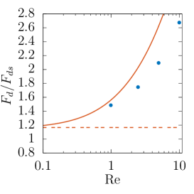
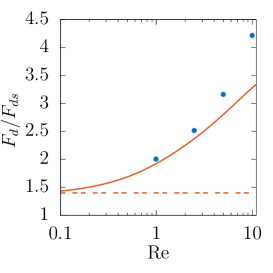
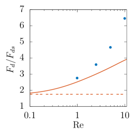
$(a)$                                        $(b)$                                        $(c)$
$\raisebox{1.5pt}{$\chi$}=2$                                    $\raisebox{1.5pt}{$\chi$}=5$                                    $\raisebox{1.5pt}{$\chi$}=10$

Figure 25: Influence of inertial effects on the drag of finite-length cylinders held perpendicular to the upstream flow. The drag is normalized by that of a sphere of same volume. Solid line: semiempirical prediction (34); dashed line: prediction (31); $\bullet$: numerical results of [12].

As Fig. 25 indicates, predictions from (34) almost match the numerical results of [12] for $\text{Re}=1$. Not surprisingly, they increasingly deviate from these results as Re increases beyond this point, over- (under-) predicting the actual drag for $\raisebox{1.5pt}{$\chi$}=2$ ($\raisebox{1.5pt}{$\chi$}=5,\,10$).

References

- Batchelor [1970] G. K. Batchelor. Slender-body theory for particles of arbitrary cross-section in Stokes flow. J. Fluid Mech., 44:419–440, 1970.
- Cox [1970] R. G. Cox. The motion of long slender bodies in a viscous fluid. Part 1. General theory. J. Fluid Mech., 44:791–810, 1970.
- Tillett [1970] J. P. K. Tillett. Axial and transverse Stokes flow past slender axisymmetric bodies. J. Fluid Mech., 44:401–417, 1970.
- Khayat and Cox [1989] R. E. Khayat and R. G. Cox. Inertia effects on the motion of long slender bodies. J. Fluid Mech., 209:435–462, 1989.
- Mackaplow and Shaqfeh [1998] M. B. Mackaplow and E. S. B. Shaqfeh. A numerical study of the sedimentation of fibre suspensions. J. Fluid Mech., 376:149–182, 1998.
- Butler and Shaqfeh [2002] J. E. Butler and E. S. G. Shaqfeh. Dynamic simulations of the inhomogeneous sedimentation of rigid fibres. J. Fluid Mech., 468:205–237, 2002.
- Shin and Koch [2005] M. Shin and D. L. Koch. Rotational and translational dispersion of fibres in isotropic turbulent flows. J. Fluid Mech., 540:143–173, 2005.
- Marchioli et al. [2010] C. Marchioli, M. Fantoni, and A. Soldati. Orientation, distribution, and deposition of elongated, inertial fibers in turbulent channel flow. Phys. Fluids, 22:033301, 2010.
- Voth and Soldati [2017] G. A. Voth and A. Soldati. Anisotropic particles in turbulence. Annu. Rev. Fluid Mech., 49:249–276, 2017.
- Ramberg [1983] S. E. Ramberg. The effects of yaw and finite length upon the vortex wakes of stationary and vibrating circular cylinders. J. Fluid Mech., 128:81–107, 1983.
- Williamson [1996] C. H. K. Williamson. Vortex dynamics in the cylinder wake. Annu. Rev. Fluid Mech., 28:477–539, 1996.
- Vakil and Green [2009] A. Vakil and S. I. Green. Drag and lift coefficients of inclined finite circular cylinders at moderate Reynolds numbers. Comput. Fluids, 38:1771–1781, 2009.
- Pierson et al. [2019] J. L. Pierson, F. Auguste, A. Hammouti, and A. Wachs. Inertial flow past a finite-length axisymmetric cylinder of aspect ratio 3: Effect of the yaw angle. Phys. Rev. Fluids, 4:044802, 2019.
- Sears [1948] W. R. Sears. The boundary layer of yawed cylinders. J. Aeronaut. Sci., 15:41–52, 1948.
- Zdravkovich [1997] M. M. Zdravkovich. Flow Around Circular Cylinders: Vol. 2: Applications. Oxford Univ. Press, 1997.
- Sanjeevi and Padding [2017] S. K. P. Sanjeevi and J. T. Padding. On the orientational dependence of drag experienced by spheroids. J. Fluid Mech., 820:R1, 2017.
- Magnaudet et al. [1995] J. Magnaudet, M. Rivero, and J. Fabre. Accelerated flows past a rigid sphere or a spherical bubble. Part 1. Steady straining flow. J. Fluid Mech., 284:97–135, 1995.
- Fabre et al. [2008] D. Fabre, F. Auguste, and J. Magnaudet. Bifurcations and symmetry breaking in the wake of axisymmetric bodies. Phys. Fluids, 20:051702, 2008.
- Auguste et al. [2010] F. Auguste, D. Fabre, and J. Magnaudet. Bifurcations in the wake of a thick circular disk. Theor. Comput. Fluid Dyn., 24:305–313, 2010.
- Auguste et al. [2013] F. Auguste, J. Magnaudet, and D. Fabre. Falling styles of disks. J. Fluid Mech., 719:388–405, 2013.
- Auguste and Magnaudet [2018] F. Auguste and J. Magnaudet. Path oscillations and enhanced drag of light rising spheres. J. Fluid Mech., 841:228–266, 2018.
- Calmet and Magnaudet [1997] I. Calmet and J. Magnaudet. Large-eddy simulation of high-Schmidt number mass transfer in a turbulent channel flow. Phys. Fluids, 9:438–455, 1997.
- Auguste [2010] F. Auguste. Instabilités de sillage et trajectoires d’un corps solide cylindrique immergé dans un fluide visqueux. PhD thesis, Université Paul Sabatier, Toulouse, France (available online at http://thesesups.ups-tlse.fr/1186/), 2010.
- Clift et al. [1978] R. Clift, J. R. Grace, and M. E. Weber. Bubbles, Drops, and Particles. Academic Press, 1978.
- Keller and Rubinow [1976] J. B. Keller and S. I. Rubinow. Slender-body theory for slow viscous flow. J. Fluid Mech., 75:705–714, 1976.
- Youngren and Acrivos [1975] G. K. Youngren and A. Acrivos. Stokes flow past a particle of arbitrary shape: a numerical method of solution. J. Fluid Mech., 69:377–403, 1975.
- Heiss and Coull [1952] J. F. Heiss and J. Coull. The effect of orientation and shape on the settling velocity of nonisometric particles in a viscous medium. Chem. Eng. Progr., 48:133–140, 1952.
- Masliyah and Epstein [1970] J. H. Masliyah and N. Epstein. Numerical study of steady flow past spheroids. J. Fluid Mech., 44:493–512, 1970.
- Lopez and Guazzelli [2017] D. Lopez and E. Guazzelli. Inertial effects on fibers settling in a vortical flow. Phys. Rev. Fluids, 2:024306, 2017.
- Roy et al. [2019] A. Roy, R. J. Hamati, L. Tierney, D. L. Koch, and G. A. Voth. Inertial torques and a symmetry breaking orientational transition in the sedimentation of slender fibres. J. Fluid Mech., 875:576–596, 2019.
- Khair and Chisholm [2018] A. S. Khair and N. G. Chisholm. A higher-order slender-body theory for axisymmetric flow past a particle at moderate Reynolds number. J. Fluid Mech., 855:421–444, 2018.
- Johnson and Patel [1999] T. A. Johnson and V. C. Patel. Flow past a sphere up to a reynolds number of 300. J. Fluid Mech., 378:19–70, 1999.
- Fröhlich et al. [2020] K. Fröhlich, M. Meinke, and W. Schröder. Correlations for inclined prolates based on highly resolved simulations. J. Fluid Mech., 901:A5, 2020.
- Pruppacher et al. [1970] H. R. Pruppacher, B. P. Le Clair, and A. E. Hamielec. Some relations between drag and flow pattern of viscous flow past a sphere and a cylinder at low and intermediate Reynolds numbers. J. Fluid Mech., 44:781–790, 1970.
- Jayaweera and Mason [1965] K. Jayaweera and B. J. Mason. The behaviour of freely falling cylinders and cones in a viscous fluid. J. Fluid Mech., 22:709–720, 1965.
- Lamb [1932] Sir H. Lamb. Hydrodynamics. Cambridge Univ. Press, 1932.
- Wachs [2009] A. Wachs. A DEM-DLM/FD method for direct numerical simulation of particulate flows: Sedimentation of polygonal isometric particles in a Newtonian fluid with collisions. Comput. Fluids, 38:1608–1628, 2009.
- Ui et al. [1984] T. J. Ui, R. G. Hussey, and R. P. Roger. Stokes drag on a cylinder in axial motion. Phys. Fluids, 27:787–795, 1984.
- Kasper et al. [1985] G. Kasper, T. Niida, and M. Yang. Measurements of viscous drag on cylinders and chains of spheres with aspect ratios between 2 and 50. J. Aerosol Sci., 16:535–556, 1985.