Continuum Percolation and Stochastic Epidemic Models
on Poisson and Ginibre Point Processes

Abstract

The most studied continuum percolation model in two dimensions is the Boolean model consisting of disks with the same radius whose centers are randomly distributed on the Poisson point process (PPP). We also consider the Boolean percolation model on the Ginibre point process (GPP) which is a typical repelling point process realizing hyperuniformity. We think that the PPP approximates a disordered configuration of individuals, while the GPP does a configuration of citizens adopting a strategy to keep social distancing in a city in order to avoid contagion. We consider the SIR models with contagious infection on supercritical percolation clusters formed on the PPP and the GPP. By numerical simulations, we studied dependence of the percolation phenomena and the infection processes on the PPP- and the GPP-underlying graphs. We show that in a subcritical regime of infection rate the PPP-based models show emergence of infection clusters on clumping of points which is formed by fluctuation of uncorrelated Poissonian statistics. On the other hand, the cumulative numbers of infected individuals in processes are suppressed in the GPP-based models.

[inst1]organization=Department of Information Physics and Computing, Graduate School of Information Science and Technology, The University of Tokyo, addlessline=Hongo, Bunkyo-ku, Tokyo 113-0033, Japan

[inst2]organization=Department of Physics, Faculty of Science and Engineering, Chuo University, addlessline=Kasuga, Bunkyo-ku, Tokyo 112-8551, Japan

1 Introduction

The study of stochastic and statistical-mechanics modeling of epidemics has a long history, and a variety of types of model has been proposed and extensively studied [1, 2, 3, 4, 5, 6, 7, 8, 9]. We choose a type of model or decide to invent a new model depending on the purpose of analysis of infection processes using mathematical models. Here we are interested in contagious disease of human beings which is spreading in a city, so spatial structures should be included in a model. In usual modeling, we choose a graph and consider that each site represents an individual and edges between neighboring sites do interactions between individuals. For example, we fix a finite but large-scale subdomain $\Lambda$ of the square lattice $\mathbb{Z}^{2}$ with some boundary condition, and to each site $x\in\Lambda$ put a random variable $\eta(x)$, which takes one of the three states, being susceptible (S), infected (I), or recovered (R) [1]. We consider the global configuration of individuals $\eta_{t}:=\{\eta_{t}(x)\}_{x\in\Lambda}$ and define a stochastic process $(\eta_{t})_{t\geq 0}$ by specifying transition rules of random variables in continuous time $t\geq 0$. The main topic of study on such a lattice SIR model [10, 11, 12, 13, 14, 15] is to clarify the dependence of the time-evolution of global configuration $\eta_{t}$ on spacial structures and relevant parameters specifying the transition rules (e.g., infection rate and recovering rate).

In a real city, however, when a serious contagious disease is spreading, citizens try to change their behavior in order to avoid contagion. A typical strategy is to keep social distancing. It is obvious that if all individuals keep the distances from their neighbors be greater than the range of contagion, then the disease will be extinct. The problem is however, that real individuals are not fixed at sites of a regular lattice, and hence they occasionally break social distancing and form groups, and it causes a risk to make infection clusters.

A system of points in a space which are randomly distributed following a specified probability law is generally called a point process. Note that this mathematical terminology means a purely static system without any time evolution [16]. The purpose of the present study is to introduce stochastic epidemic models of individuals whose locations are given by a random point process, and to clarify dependence of the infection processes on the underlying graph $\mathcal{G}$ given by a point process.

Figure 1: Typical realizations of point configurations in the Poisson point process (PPP) in the left, and in the Ginibre point process (GPP) in the right. In both figures, the total number of points is 200.

In the present paper we use two distinct point processes on a plane $\mathbb{R}^{2}$ to define underlying graphs; the Poisson point process (PPP) and the Ginibre point process (GPP) [17]. The left figure of Fig. 1 shows a typical realization of 200 points of the PPP, while the right one shows that of the GPP. The GPP is realized as a bulk scaling limit of eigenvalue distributions on a complex plane $\mathbb{C}$ of Gaussian complex random matrices, which has been extensively studied in random matrix theory [18, 19]. It is a typical two-dimensional example of a large family of repelling point processes called the determinantal (fermion) point processes [20, 21, 22, 23, 24, 25]. On the other hand, there is no correlation among points in the PPP. In this sense, the PPP can be said to be a uniform distribution of point process. We observe in the left figure of Fig. 1, however, that clumping of points and vacant spaces happen to occur. In the PPP the variance of the number of points included in the disk with center $x\in\mathbb{R}^{2}$ and radius $r>0$, $B_{r}(x):=\{y\in\mathbb{R}^{2}:|y-x|<r\}$, is proportional to $r^{2}$; that is, the fluctuation of the number of points in a disk is in the same order with the total number of points in it. In the GPP, due to the repulsive interactions among points, the variance of the number of points in $B_{r}(x)$ is only proportional to $r$ in $r\to\infty$. (Note that both point processes are translationally invariant and then the center $x$ of disk is arbitrary in the above assertions.) Such a suppression of number fluctuations is a common feature of deterministic lattices, determinantal point processes, and other correlated particle systems, and called hyperuniformity [26, 27]. The GPP will mimic locations of citizens in a city who try to keep social distancing, while the PPP will do a society in which such a strategy to avoid contagion is not adopted at all.

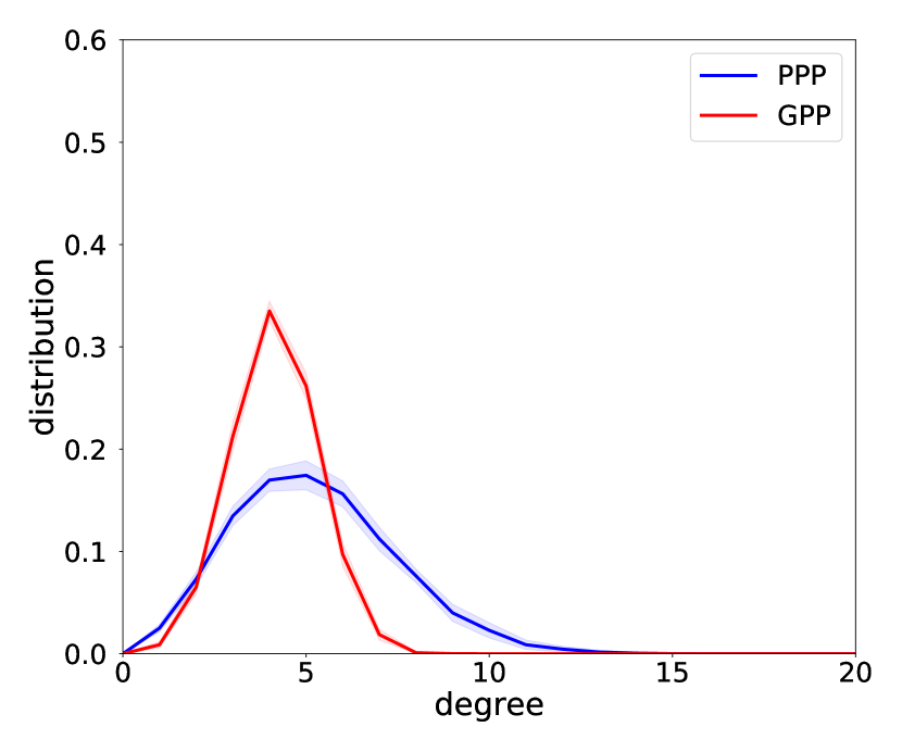
Figure 2: Distributions of degree of each points in the PPP-underlying graph $\mathcal{G}^{\rm PPP}$ and the GPP-underlying graph $\mathcal{G}^{\rm GPP}$. Solid lines show the means of ten distinct samples of random graphs and shaded strips show the standard deviations of them. The mean values of degree are given by 5.23 for $\mathcal{G}^{\rm PPP}$ and 4.15 for $\mathcal{G}^{\rm GPP}$.

We express the range of infection by a parameter $r>0$ and consider an infection process such that only if the distance between two individuals is less than $2r$, contagion can occur. In other words, the maximum set of individuals who have the possibility to be infected is given by a set of points $x$ each of which has at least one neighboring point $y$ such that $B_{r}(x)\,{\cap}\,B_{r}(y)\not=\emptyset$. Such a set is known as a percolation cluster of the Boolean percolation model or the standard Gilbert disk model [28] in the continuum percolation theory [29, 30, 31, 32, 33]. We have numerically generated typical samples of large percolation clusters on the PPP and the GPP and regarded them as a pair of distinct underlying graphs $\mathcal{G}^{\rm PPP}$ and $\mathcal{G}^{\rm DPP}$ for our epidemic models. In order to compare essential differences between them, we have imposed the condition on the Boolean percolation models from which $\mathcal{G}^{\rm PPP}$ and $\mathcal{G}^{\rm GPP}$ are obtained such that the filling factors, defined by (4) below, take the same value $\kappa$. The specified value of $\kappa$ is greater than the critical values of percolation transitions on the PPP and on the GPP; $\kappa>\kappa_{\rm c}^{\rm PPP}>\kappa_{\rm c}^{\rm GPP}$. One of the differences between these two graphs is represented by the distributions of degrees of each point, where the degree of each point means the number of neighboring points in the graph. As shown by Fig. 2, points with larger values of degrees are realized in $\mathcal{G}^{\rm PPP}$ compared to $\mathcal{G}^{\rm GPP}$.

We have numerically studied the SIR models [1] on $\mathcal{G}^{\rm PPP}$ and on $\mathcal{G}^{\rm GPP}$ starting from the same initial configuration with only one infected (I) individual at a randomly chosen point in a field of susceptible (S) individuals. The infection process $\mathrm{S}\to\mathrm{I}$ takes place with rate $\lambda\Psi(n)$ and the recovering $\mathrm{I}\to\mathrm{R}$ with rate $\mu\equiv 1$, where the infectivity $\lambda>0$, $\Psi$ is a positive function, and $n$ gives the total number of neighbors who are infected. The recovered (R) individuals are stable and never to be infected again. If $\lambda$ is large, infection spreads more efficiently on $\mathcal{G}^{\rm GPP}$ than on $\mathcal{G}^{\rm PPP}$ due to the hyperuniformity of the GPP. In such a case, the strategy such as keeping social distancing does not work.

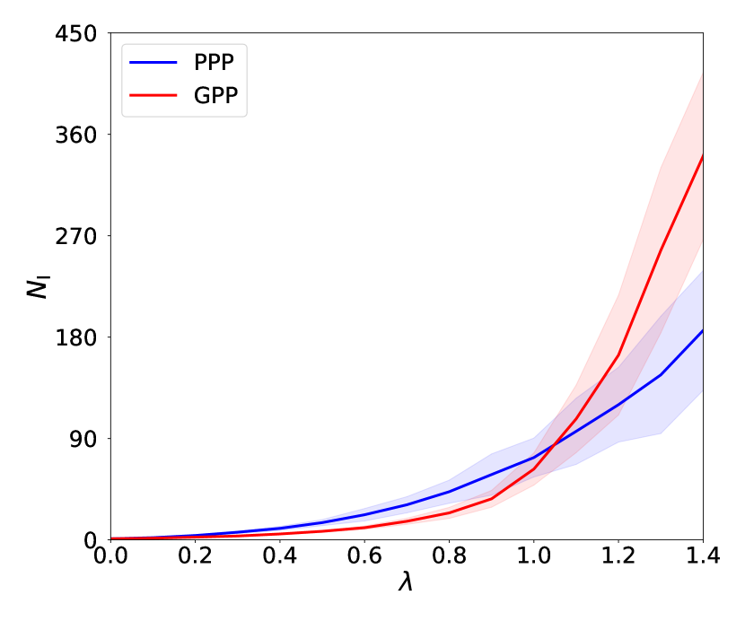
Figure 3: For each underlying graph $\mathcal{G}$ we performed 100 runs of the SIR models in which the infection rate is given by $\lambda\widehat{\Psi}(n)$ with a quadratic function $\widehat{\Psi}(n)=n^{2}$, and $n$ denotes the number of infected neighbors. We defined the cumulative number of infected individuals $\mathcal{N}_{\mathrm{I}}$ by the mean value of the 100 runs. The quenched averages $\langle\mathcal{N}_{\mathrm{I}}\rangle$ over ten distinct samples of $\mathcal{G}$ are shown versus $\lambda$ for the PPP-based model by a blue curve and for the GPP-based model by a red curve. The standard deviations in the ten samples are shown by shaded strips around the curves. We find a crossing point at $\lambda_{*}\simeq 1.0$ of these two curves.

In the present work, we are interested in the situation in which $\lambda$ is relatively small and infection clusters do not spread over large-scale. The main assertion of the preset paper is that in this case the cumulative number of infected individuals $\mathcal{N}_{\mathrm{I}}$ in an infection process can be suppressed in the GPP-based model compared to the PPP-based model. It was confirmed that this phenomenon is realized in the simple ‘linear model’ in which $\Psi(n)=n,n\in\mathbb{N}:=\{1,2,\dots\}$, and then we studied its dependence on the functional form of $\Psi(n)$. Figure 3 shows dependence of $\mathcal{N}_{\mathrm{I}}$ on $\lambda$ for the ‘quadratic model’ in which we assume $\widehat{\Psi}(n)=n^{2},n\in\mathbb{N}$. In each sample of $\mathcal{G}$, the SIR model with a given value of $\lambda$ was simulated 100 times using the Gillespie algorithm [34, 35, 36] and $\mathcal{N}_{\mathrm{I}}$ is defined by the mean value of 100 runs. Then we evaluate the average $\langle\mathcal{N}_{\mathrm{I}}\rangle$ and the standard deviation over ten distinct samples of $\mathcal{G}$. This procedure should be regarded as quenched averaging of the SIR model on random environments given by underlying graphs $\mathcal{G}$. We find a special value $\lambda_{*}\simeq 1.0$ such that $\langle\mathcal{N}_{\mathrm{I}}^{\rm PPP}\rangle>\langle\mathcal{N}_{\mathrm{I}}^{\rm GPP}\rangle$ if $0<\lambda<\lambda_{*}$, while $\langle\mathcal{N}_{\mathrm{I}}^{\rm PPP}\rangle<\langle\mathcal{N}_{\mathrm{I}}^{\rm GPP}\rangle$ if $\lambda>\lambda_{*}$. Since $\lambda_{*}$ is much less than the critical infection rate $\lambda_{\rm c}$, infection processes cease sooner or later and final configurations are expressed by a confined and connected domain consisting of $\mathrm{R}$-individuals embedded in a field of $\mathrm{S}$-individuals. Typical final configurations are shown in Fig. 4 for the PPP-based model in the left and for the GPP-based model in the right. We observe an accumulation of $\mathrm{R}$-individuals on a clumping of points in $\mathcal{G}^{\rm PPP}$. Emergence of such infection clusters is suppressed in the model on $\mathcal{G}^{\rm GPP}$ when $\lambda<\lambda_{*}$. Remember that there is no correlation at all in the PPP and clumping of points is formed accidentally. This implies that infection clusters can be caused by fluctuation of point processes even though the infectivity $\lambda$ is relatively small.

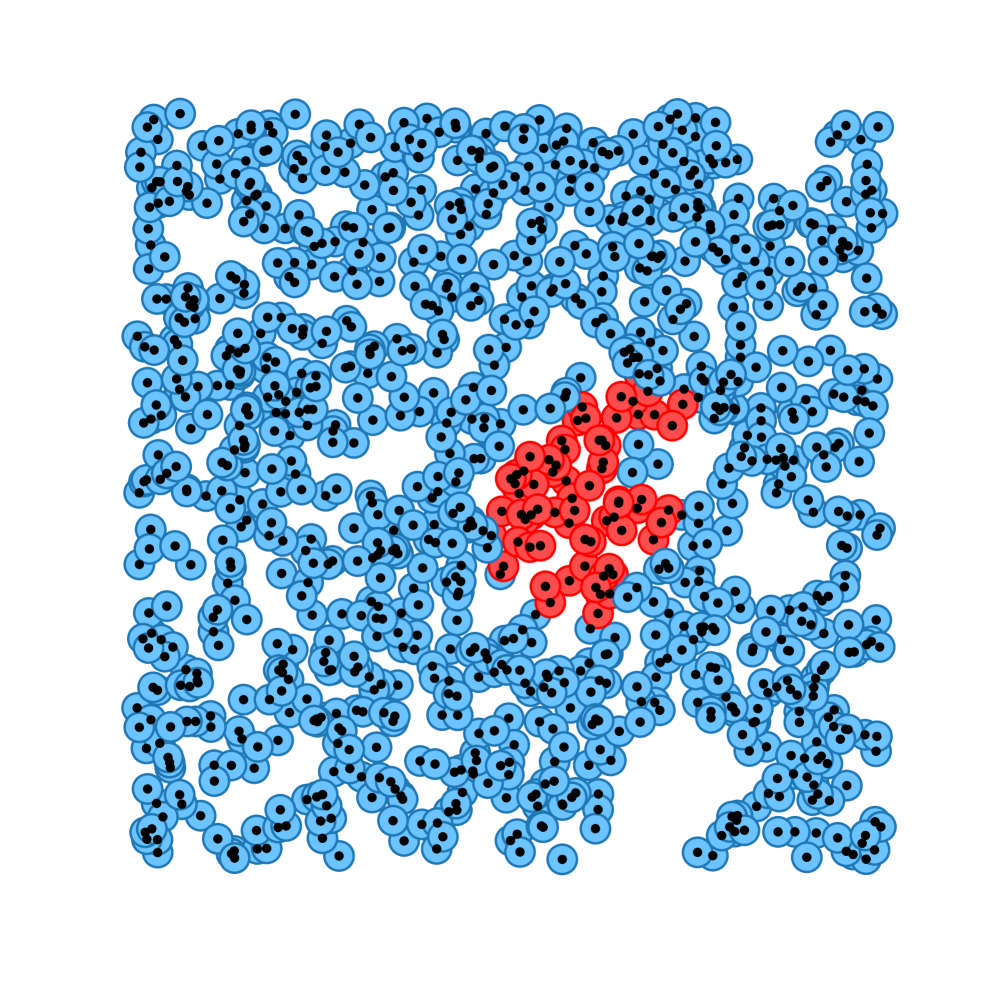
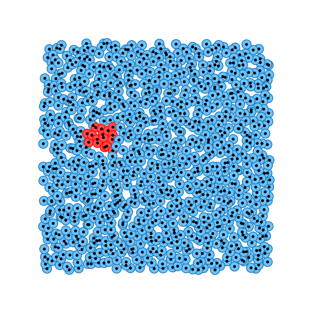
Figure 4: Examples of final configuration of the SIR model on $\mathcal{G}^{\rm PPP}$ in the left and on $\mathcal{G}^{\rm GPP}$ in the right. Here $\lambda=0.8$ and the quadratic function $\widehat{\Psi}(n)=n^{2},n\in\mathbb{N}$ is assumed. Blue and red disks show $\mathrm{S}$- and $\mathrm{R}$-individuals, respectively. The numbers of $\mathrm{R}$-individuals in the final configurations, which are equal to $\mathcal{N}_{\mathrm{I}}$, are 68 in the left and 18 in the right, respectively.

The paper is organized as follows. In Section 2 first we give the mathematical definitions of the PPP and the GPP, and then the Boolean percolation models on them are introduced. We briefly explain the percolation transition at the critical filling factor $\kappa_{\rm c}$, and we use an infinite percolation cluster which can appear in the supercritical phase $\kappa>\kappa_{\rm c}$ as a underlying graph $\mathcal{G}$ for our epidemic models. We define the SIR models with contagious infections on $\mathcal{G}$. We report our numerical results on the Boolean percolation models on the PPP and the GPP in Section 3. Numerical estimations of $\kappa_{\rm c}^{\rm PPP}$ and $\kappa_{\rm c}^{\rm GPP}$ are given there. Section 4 is devoted to the simulation results of the SIR models and dependence of infection processes on the two distinct underlying graphs $\mathcal{G}^{\rm PPP}$ and $\mathcal{G}^{\rm GPP}$ is studied. We performed simulations of the SIR models by modifying the function $\Psi$. Dependence of the ratio $\langle\mathcal{N}_{\mathrm{I}}^{\rm GPP}\rangle/\langle\mathcal{N}_{\mathrm{I}}^{\rm PPP}\rangle$ on $\lambda$ is shown for each version of model, which will help us to understand the suppression mechanism of infection clusters in the GPP-based model in the parameter regime $0<\lambda<\lambda_{*}$. Concluding remarks are listed out in Section 5.

2 The Models and their Basic Properties

2.1 The Poisson point process (PPP)

For a domain $A\subset\mathbb{R}^{2}$, its area is denoted by $|A|$. So if $A$ is bounded, then $|A|<\infty$. We write the Poisson point process (PPP) on $\mathbb{R}^{2}$ as $\Xi^{\rm PPP}$. $\Xi^{\rm PPP}$ is a counting measure of randomly distributed points on $\mathbb{R}^{2}$ such that, for any bounded $A\subset\mathbb{R}^{2}$, the number of points included in $A$ is given by a random variable $\Xi^{\rm PPP}(A)$. $\Xi^{\rm PPP}$ with intensity $\alpha>0$ satisfies the following [16, 29].

1. For mutually disjoint bounded domains $A_{1},\dots,A_{m}$, $m\in\mathbb{N}$; that is, $A_{j}\cap A_{k}=\emptyset$, $\forall j\not=k$, the random variables $\Xi^{\rm PPP}(A_{1}),\dots,\Xi^{\rm PPP}(A_{m})$ are mutually independent.

2. For any bounded domain $A\subset\mathbb{R}^{2}$,

   $$\mathrm{P}(\Xi^{\rm PPP}(A)=\ell)=e^{-\alpha|A|}\frac{\alpha^{\ell}|A|^{\ell}}{\ell!},$$ (1)

   $\ell\in\mathbb{N}_{0}:=\{0,1,\dots\}$.

By (1), the mean value of $\Xi^{\rm PPP}(A)$ is calculated as

$$\langle\Xi^{\rm PPP}(A)\rangle :=\sum_{\ell=0}^{\infty}\ell\mathrm{P}(\Xi^{\rm PPP}(A)=\ell)$$

$$=e^{-\alpha|A|}\sum_{\ell=0}^{\infty}\ell\frac{\alpha^{\ell}|A|^{\ell}}{\ell!}=\alpha|A|,$$

for $A\subset\mathbb{R}^{2}$ with $|A|<\infty$, and hence the density $\rho^{\rm PPP}$ is equal to the intensity,

$$\rho^{\rm PPP}:=\frac{\langle\Xi^{\rm PPP}(A)\rangle}{|A|}=\alpha.$$

Similarly, the variance of the number of points included in a bounded domain $A\subset\mathbb{R}^{2}$ is calculated as

$$\mathrm{var}(\Xi^{\rm PPP}(A)):=\langle(\Xi^{\rm PPP}(A)-\langle\Xi^{\rm PPP}(A)\rangle)^{2}\rangle=\alpha|A|,$$

which implies that as $|A|\to\infty$ the variance grows in the same order of the mean of the number of points,

$$\lim_{|A|\to\infty}\frac{\mathrm{var}(\Xi^{\rm PPP}(A))}{\langle\Xi^{\rm PPP}(A)\rangle}=1.$$

2.2 The Ginibre point process (GPP)

Here we identify the real two-dimensional plane $\mathbb{R}^{2}$ with a complex plane $\mathbb{C}$. For $z=x+iy\in\mathbb{C}$ with $i:=\sqrt{-1}$, $x,y\in\mathbb{R}$, we write $\overline{z}:=x-iy$, $dz=dxdy$. For $z=x+iy,z^{\prime}=x^{\prime}+iy^{\prime}\in\mathbb{C}$, $z\overline{z^{\prime}}=(xx^{\prime}+yy^{\prime})-i(xy^{\prime}-x^{\prime}y)$; in particular $|z|^{2}:=z\overline{z}=x^{2}+y^{2}$.

Consider an $L\times L$ matrix $M_{L}=(m_{jk})_{1\leq j,k\leq L}$, $L\in\mathbb{N}$, whose entries are independently and identically distributed (i.i.d.) complex Gaussian random variable with mean zero and variance $\sigma^{2}$;

$$\mathrm{P}(m_{jk}\in dz)=\frac{1}{\pi\sigma^{2}}e^{-|z|^{2}/\sigma^{2}}dz,\quad j,k=1,2,\dots,L.$$ (2)

We can prove that the eigenvalues of $M_{L}$, $\{Z_{j}\}_{j=1}^{L}$ in uniform random order, obey the following joint probability distribution,

$$\mathrm{P}(Z_{1}\in dz_{1},\dots,Z_{L}\in dz_{L})$$

$$\quad=\frac{1}{\pi^{L}\sigma^{L(L-1)}\prod_{\ell=1}^{L}\ell!}e^{-\sum_{\ell=1}^{L}|z_{\ell}|^{2}/\sigma^{2}}$$

$$\qquad\times\prod_{1\leq j<k\leq L}|z_{k}-z_{j}|^{2}dz_{1}\cdots dz_{L},$$

$z_{1},\dots,z_{L}\in\mathbb{C}$. The factor $\prod_{1\leq j<k\leq L}|z_{k}-z_{j}|^{2}$ gives repulsive correlation between any pair of points.

Such a correlated point process is generally characterized by correlation functions [18, 19, 25]. For a point process $\Xi$, the $n$-th correlation function $\rho_{n}$, $n\in\mathbb{N}$, is defined as the following. Again we consider mutually disjoint bounded domains $A_{1},\dots,A_{m}\subset\mathbb{R}^{2}$, $m\in\mathbb{N}$. For any set of integers $k_{1},\dots,k_{m}\in\mathbb{N}_{0}$ satisfying $\sum_{\ell=1}^{m}k_{\ell}=n\in\mathbb{N}_{0}$,

$$\left\langle\prod_{\ell=1}^{m}\frac{\Xi(A_{\ell})}{(\Xi(A_{\ell})-k_{\ell})!}\right\rangle$$

$$\quad=\int_{A_{1}^{k_{1}}\times\cdots\times A_{m}^{k_{m}}}\rho_{n}(z_{1},\dots,z_{n})dz_{1}\cdots dz_{n},$$

where if $\Xi(A_{\ell})-k_{\ell}<0$, we interpret $\Xi(A_{\ell})!/(\Xi(A_{\ell})-k_{\ell})!=0$. For any $L\in\mathbb{N}$, the eigenvalues $\{Z_{j}\}_{j=1}^{L}$ provides a determinantal point process (DPP) in the sense that any correlation function is expressed by a determinant

$$\rho^{L}_{n}(z_{1},\dots,z_{L})=\det_{1\leq j,k\leq L}[K_{L}(z_{j},z_{k})],$$

$n\in\{1,2,\dots,L\}$. All correlation functions are specified by a two-point function called the correlation kernel, and in the present case it is given by [17]

$$K_{L}(z,z^{\prime})=\frac{1}{\pi\sigma^{2}}e^{-(|z|^{2}+|z^{\prime}|^{2})/2\sigma^{2}}\sum_{\ell=0}^{L-1}\frac{1}{\ell!}\left(\frac{z\overline{z^{\prime}}}{\sigma^{2}}\right)^{\ell}.$$

As $L\to\infty$, this function converges to

$$K^{\rm GPP}(z,z^{\prime})=\frac{1}{\pi\sigma^{2}}e^{-(|z|^{2}+|z^{\prime}|^{2})/2\sigma^{2}+z\overline{z^{\prime}}/\sigma^{2}},$$

$z,z^{\prime}\in\mathbb{C}$, which is hermitian; $\overline{K^{\rm GPP}(z,z^{\prime})}=K^{\rm GPP}(z^{\prime},z)$. This limit correlation kernel defines a DPP with an infinite number of points on $\mathbb{R}^{2}$ through the correlation functions $\rho^{\rm GPP}_{n}(z_{1},\dots,z_{n})=\det_{1\leq j,k\leq n}[K^{\rm GPP}(z_{j},z_{k})]$, $n\in\mathbb{N}$. This infinite point process is called the Ginibre point process (GPP) and denoted by $\Xi^{\rm GPP}$ [17, 18, 23, 24, 19].

The GPP is a uniform point process with density

$$\rho^{\rm GPP}=\rho_{1}^{\rm GPP}=K^{\rm GPP}(z,z)=\frac{1}{\pi\sigma^{2}}.$$

The two-point correlation function is given by

$$\rho^{\rm GPP}_{2}(z,z^{\prime}) =\det\left[\begin{array}[]{ll}K^{\rm GPP}(z,z)&K^{\rm GPP}(z,z^{\prime})\cr K^{\rm GPP}(z^{\prime},z)&K^{\rm GPP}(z^{\prime},z^{\prime})\end{array}\right]$$

$$=K^{\rm GPP}(z,z)K^{\rm GPP}(z^{\prime},z^{\prime})-|K^{\rm GPP}(z,z^{\prime})|^{2}$$

$$=(\rho^{\rm GPP})^{2}-|K^{\rm GPP}(z,z^{\prime})|^{2},$$

$z,z^{\prime}\in\mathbb{C}$. The inequality $\rho^{\rm GPP}_{2}(z,z^{\prime})-(\rho^{\rm GPP})^{2}<0$ holds and it implies negative correlation; that is, $\Xi^{\rm GPP}$ is a repelling point process.

It was proved by [23] that

$$\mathrm{var}(\Xi^{\rm GPP}(B_{r}))\sim\frac{r}{\sqrt{\pi}\sigma}\quad\mbox{as $r\to\infty$}.$$

This implies that the GPP is hyperuniform in the sense [26],

$$\frac{\mathrm{var}(\Xi^{\rm GPP}(B_{r}))}{\langle\Xi^{\rm GPP}(B_{r})\rangle}\propto r^{-1}\to 0\quad\mbox{as $r\to\infty$},$$

as mentioned in Section 1. See also [27].

2.3 The Boolean percolation model and critical filling factor

Let $\Xi$ be a point process on $\mathbb{R}^{2}$. So far $\Xi$ has been considered as a measure of random points on $\mathbb{R}^{2}$; for instance, given a bounded domain $A\subset\mathbb{R}^{2}$, $\Xi(A)$ counts the number of points included in $A$. Here we regard a point process simply as a set of points. Corresponding to $\Xi$, we define

$$\widehat{\Xi}:=\{x\in\mathbb{R}^{2}:\Xi(\{x\})\geq 1\}.$$ (3)

Notice that, by negative correlation, there is no multiple points in the GPP; $\Xi^{\rm GPP}(\{x\})\in\{0,1\}$, with probability one [24]. So the inequality ‘$\geq$’ in (3) can be replaced by the equality ‘$=$’ for the GPP.

Now we introduce a real number $r>0$. For two points $x,y\in\widehat{\Xi}$, if the Euclidean distance $|x-y|<2r$, then we say that $x$ and $y$ are neighbors of each other. We place disks of radius $r$ around each point; $B_{r}(x),x\in\widehat{\Xi}$. Then if and only if $B_{r}(x)\cap B_{r}(y)\not=\emptyset$, the two points $x$ and $y$ are neighbors. Two points $x$ and $y$ are connected if there is a finite sequence of points $x_{0},x_{1},\dots,x_{n}\in\widehat{\Xi}$ such that $x_{0}=x,x_{n}=y$ and $x_{j+1}$ is a neighbor of $x_{j}$, $j=0,1,\dots,n-1$. The above defines the Boolean percolation model on the point process $\widehat{\Xi}$ with radius $r$ [28, 29, 30, 31, 32, 33].

The maximal connected components are called percolation clusters. The size of a percolation cluster is the number of points in $\widehat{\Xi}$ included in the percolation cluster. We say that the system percolates if there is at least one infinite cluster, whose size is infinity [37, 30]. The uniqueness of the infinite cluster with probability one was proved for the Boolean percolation on the PPP and the GPP [29, 30, 33]. The probability that the system percolates is called the percolation probability and denoted by $\Theta$. In the present Boolean percolation model on $\mathbb{R}^{2}$, $\Theta$ is a function of the product of the density $\rho$ of the point process $\widehat{\Xi}$ and the area of a disk $a=\pi r^{2}$,

$$\kappa:=\rho a=\rho\pi r^{2},$$ (4)

which is called the filling factor [38]. There is a unique critical value of filling factor $\kappa_{\rm c}$ such that $\Theta(\kappa)=0$, if $\kappa\leq\kappa_{\rm c}$. In the supercritical phase $\kappa>\kappa_{\rm c}$, $\Theta(\kappa)>0$, and in the vicinity of $\kappa_{\rm c}$, $\Theta(\kappa)$ behaves as [37],

$$\Theta(\kappa)\simeq\mbox{const.}\times(\kappa-\kappa_{\rm c})^{\beta},\quad\kappa\gtrsim\kappa_{\rm c}$$ (5)

with a critical exponent $\beta$. It has been argued that continuum percolation and lattice percolation will belong to the same universality class [39, 40]. The critical exponent of the percolation models on usual planar lattices is known as $\beta=5/36=0.1388\cdots$ [37].

2.4 The SIR models on an infinite percolation cluster

Now we construct epidemic models on percolation clusters. By definition of neighbors given above, a sequence of contagion should be limited within the percolation cluster. We set $\kappa>\kappa_{\rm c}$ and consider an infinite cluster $\mathcal{G}$ as a underlying graph on which our epidemic model is constructed. As will be explained in Section 3 below, we will perform numerical simulations on finite point processes put on a finite two-dimensional region with the periodic boundary condition. In such a case we will use the largest cluster found in the finite system as an underlying graph. If we consider the SIR models starting from one infected individual with weak infectivity, $\lambda\ll\lambda_{\rm c}$, an infection region is confined in a relatively small area. Then the finite-size effect of underlying graph will be irrelevant.

Assume that an underlying graph is given by $\mathcal{G}$. At each point $x\in\mathcal{G}$, we put a random variable $\eta(x)\in\{\mathrm{S},\mathrm{I},\mathrm{R}\}$. We consider a continuous-time Markov process, $(\eta_{t})_{t\geq 0}$, where $\eta_{t}:=\{\eta_{t}(x)\}_{x\in\mathcal{G}}$. The transition mechanism is specified by two positive parameters $\lambda,\mu$ and a positive function $c(x,\eta)$ as

$$\mathbf{P}^{\eta}(\eta_{t}(x)=\mathrm{I},\eta(x)=\mathrm{S}) =\lambda c(x,\eta)t+\mathrm{o}(t),$$

$$\mathbf{P}^{\eta}(\eta_{t}(x)=\mathrm{R},\eta(x)=\mathrm{I}) =\mu t+\mathrm{o}(t)\quad\mbox{as $t\to 0$},$$

where $\mathbf{P}^{\eta}$ denotes the probability in this Markov process starting from the configuration $\eta$. That is, if an individual at point $x$ is in the susceptible (S) state, it is infected (I) at rate $\lambda c(x,\eta)$, while if it is infected (I), it becomes recovered at rate $\mu$. Note that once $\eta(x)=\mathrm{R}$, the state does not change forever. We require that only one-variable-change happens in each transition; that is, $\mathbf{P}^{\eta}(\eta_{t}(x)\not=\eta(x),\eta_{t}(y)\not=\eta(y))=\mathrm{o}(t)$ as $t\to 0$ for each $x,y\in\mathcal{G}$ with $x\not=y$ given a configuration $\eta$ on $\mathcal{G}$. See [4, 6] for the mathematical construction of interacting particle systems.

Now we introduce a positive function $\Psi(n)$, $n\in\mathbb{N}_{0}$ and specify the function $c(x,\eta)$ as follows,

$$c(x,\eta)=\Psi\left(\sum_{y:|y-x|<2r}1_{(\eta(y)=\mathrm{I})}\right),$$ (6)

where $1_{(\omega)}$ is the indicator function of an event $\omega$; $1_{(\omega)}=1$ if $\omega$ is satisfied and $1_{(\omega)}=0$ otherwise. On an infinite percolation cluster $\mathcal{G}$, we can discuss the percolation problem for an infection cluster consisting of $\mathrm{I}$-individuals and $\mathrm{R}$-individuals. When $\Psi(n)$ is an increasing function of $n$, the percolation probability of infection cluster $\Theta^{\rm SIR}$ on $\mathcal{G}$ is increasing in $\lambda$. Moreover, a unique critical value $\lambda_{\rm c}$ is defined so that [10, 41, 11, 12, 15]

$$\Theta^{\rm SIR}(\lambda)=0,\quad\mbox{if $\lambda\leq\lambda_{\rm c}$},$$

$$\Theta^{\rm SIR}(\lambda)>0,\quad\mbox{if $\lambda>\lambda_{\rm c}$}.$$

For each SIR model with a specified $\Psi$, it is expected that $\lambda_{\rm c}$ does not depend on each sample of infinite underlying graph $\mathcal{G}$ and it is determined only by the filling factor $\kappa$ of the Boolean percolation model from which $\mathcal{G}$ is defined.

When $\Psi(n)=n$, the infection rate is just given by the total number of infected neighbors multiplied by $\lambda$. We call this case the linear model.

3 Numerical Simulations and Results of the Percolation Problem

3.1 Percolation probability and critical filling factor

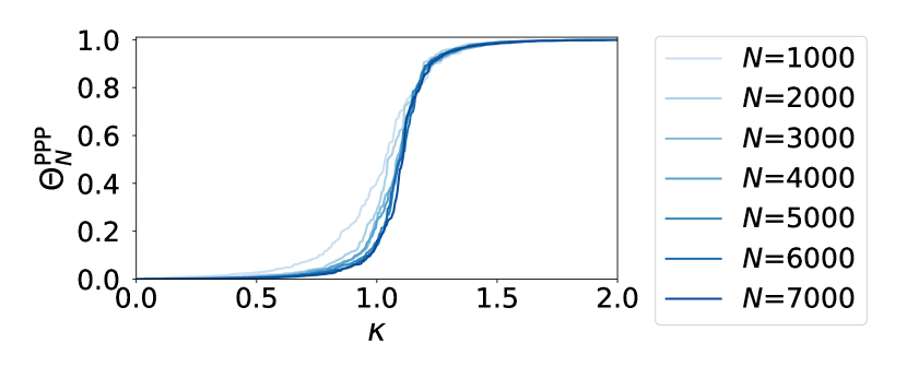
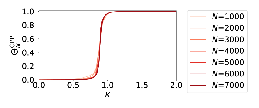
Figure 5: Approximation curves of the percolation probability, $\Theta^{\rm PPP}_{N}$ (resp. $\Theta^{\rm GPP}_{N}$) are plotted in the top (resp. bottom) figure with respect to the filling factor $\kappa$ for several values of $N$.

It is easy to generate samples of the PPP with finite number of points $N$ in the unit square $[0,1]^{2}$ on $\mathbb{R}^{2}$, since it is a uniform point process without any correlation. The obtained point process is denoted by $\Xi^{\rm PPP}_{N}$ which has density $\rho^{\rm PPP}_{N}=N$. For the GPP, we have first prepared $L\times L$ random matrices with $L=2N$, whose complex entries are i.i.d. and following (2) with $\sigma^{2}=2$; that is, the real and the imaginary parts of each entry are i.i.d. real standard Gaussian random variables. Then we calculated $L=2N$ complex eigenvalues and plot them on $\mathbb{C}$. We have confirmed that the eigenvalues follows the circle law [18, 19]. That is, almost all of them are distributed in a disk around the origin with radius $\sqrt{2N}$, and within the disk, except for a very narrow region near the edge of the disk (i.e., near the circumference), their distribution is uniform. Here we have used only the point distribution in the central $\sqrt{\pi N}\times\sqrt{\pi N}$ square and performed a scale change by factor $1/\sqrt{\pi N}$ to obtain a point process $\Xi^{\rm GPP}_{N}$ on the unit square $[0,1]^{2}$ having density $\rho^{\rm GPP}_{N}=N$, which approximates the GPP. In this way we have generated samples of finite approximations $\Xi^{\rm PPP}_{N}$ and $\Xi^{\rm GPP}_{N}$ with seven different $N$ from $N=1000$ to $N=7000$.

For each finite point processes $\Xi^{\rm PPP}_{N}$, $\Xi^{\rm GPP}_{N}$ plotted on $[0,1]^{2}$, we impose the periodic boundary condition. Then the percolation probability $\Theta$ is approximated by the ratio $\Theta_{N}$ of the number of points included in the largest cluster to the total number of points $N$ [37]. Figure 5 shows the curves of $\Theta_{N}$ as functions of the filling factor $\kappa$ defined by (4) for the Boolean percolation models on $\Xi^{\rm PPP}_{N}$ in the top and on $\Xi^{\rm GPP}_{N}$ in the bottom figure, respectively, with increasing $N$ from 1000 to 7000 by 1000.

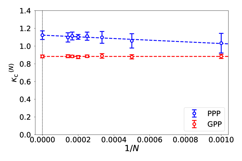
Figure 6: Approximate values of critical filling factor $\kappa_{\rm c}^{{\rm PPP}(N)}$ and $\kappa_{\rm c}^{{\rm GPP}(N)}$ are plotted versus $1/N$. The error bars are estimated by ten samples of finite point processes of each size $N$.

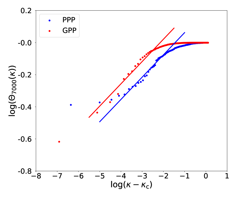
Figure 7: The least-square linear regression was applied to the log-log plot of (5) with $\beta=5/36$ for the data of the largest systems with $N=7000$. The evaluated values of the critical filling factors are $\kappa_{\rm c}^{\rm PPP}=1.13$ and $\kappa_{\rm c}^{\rm GPP}=0.894$, respectively.

For each curve $\Theta_{N}$, an approximate value of critical filling factor, denoted by $\kappa_{\rm c}^{(N)}$, is defined by the value of $\kappa$ at which the numerical value of $d\Theta_{N}(\kappa)/d\kappa$ attains the maximum. We plot $\kappa_{\rm c}^{{\rm PPP}(N)}$ and $\kappa_{\rm c}^{{\rm GPP}(N)}$ versus $1/N$ in Fig. 6. They behave well as $\kappa_{\rm c}^{(N)}\simeq{\rm const.}/N\,+\,\kappa_{\rm c}$ as $N\to\infty$, and we obtained the following estimations for the critical values,

$$\kappa_{\rm c}^{\rm PPP} =1.12\pm 0.05,$$

$$\kappa_{\rm c}^{\rm GPP} =0.884\pm 0.016.$$ (7)

Using the data of the largest systems with $N=7000$, we performed another method to evaluate $\kappa_{\rm c}$ as follows. We assumed the critical behavior (5) of $\Theta(\kappa)$ with the exponent $\beta=5/36$ and applied the least-square linear regression to log-log plots of the data $\Theta_{7000}(\kappa)$ versus $\kappa-\kappa_{\rm c}$, where $\kappa_{\rm c}$ is a fitting parameter and the slope of fitting line is fixed to be $5/36$. Figure 7 shows the best fitting, which gives the estimates,

$$\kappa_{\rm c}^{\rm PPP}=1.13,\quad\kappa_{\rm c}^{\rm GPP}=0.894.$$ (8)

The present evaluations of $\kappa_{\rm c}^{\rm PPP}$ are consistent with the value reported in [38] evaluated using efficient algorithms [42, 43, 44, 45], $\kappa_{\rm c}^{\rm PPP}=1.12808737(6)$. To the best of the knowledge of the present authors, the above are the first numerical estimations of the critical filling factor $\kappa_{\rm c}^{\rm GPP}$ of the Boolean percolation model on the GPP.

3.2 Largest percolation clusters as underlying graphs for the SIR models

From now on we consider the supercritical percolation models. We fix the filling factor of the Boolean percolation model as $\kappa=1.3$, which is greater than the both critical values $\kappa_{\rm c}^{\rm PPP}$ and $\kappa_{\rm c}^{\rm GPP}$ evaluated as (7) and (8). We pick up only the largest cluster found in the Boolean percolation models simulated as explained above. Figure 8 shows the typical samples for the PPP in the left and the GPP in the right. In the both systems, the total number of disks in the largest cluster is 1000. We will use such a pair of percolation clusters made from point processes as the underlying graphs $\mathcal{G}$ of our contagious epidemic model of the SIR type.

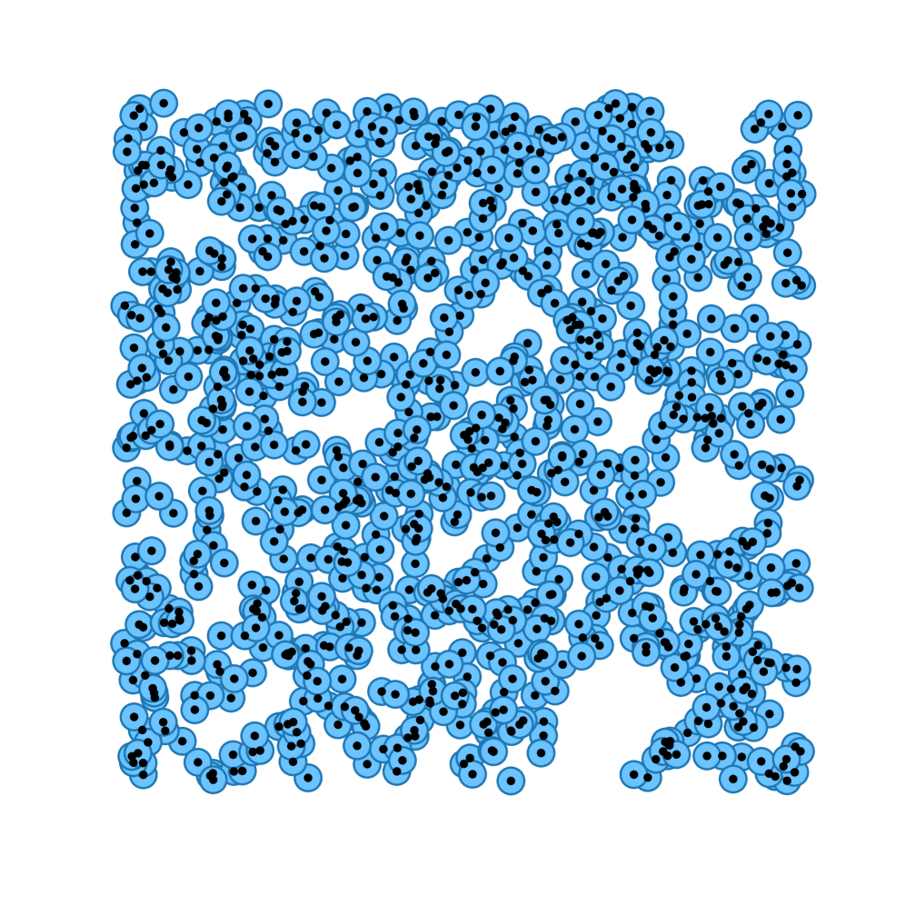
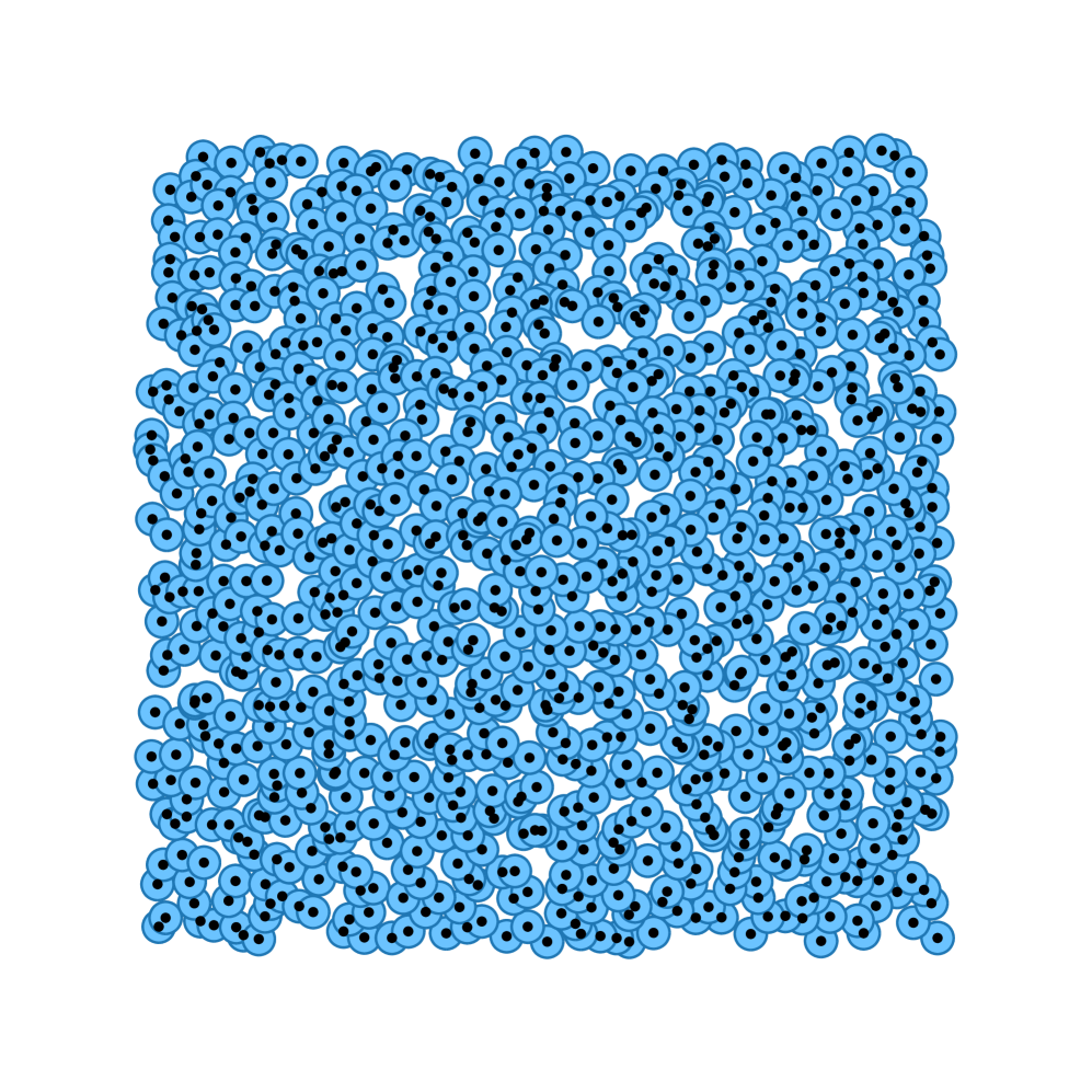
Figure 8: A pair of samples of underlying graphs for our contagious epidemic models. The left graph $\mathcal{G}^{\rm PPP}_{N}$ (resp. the right graph $\mathcal{G}^{\rm GPP}_{N}$) is a finite approximation with $N=1000$ of an infinite percolation cluster $\mathcal{G}^{\rm PPP}$ (resp. $\mathcal{G}^{\rm GPP}$).

Although the filling factor $\kappa$ is the same in the original Boolean percolation models, it is obvious that these two kinds of $\mathcal{G}_{N}$ obtained from them are different from each other. The difference can be clearly shown by the distributions of degree of each point, which was already shown by Fig. 2 and explained in Section 1.

4 Numerical Simulations and Results of the SIR Models

4.1 The Gillespie algorithm

Since time scale is arbitrary in computer simulations, we can put the recovering rate $\mu\equiv 1$ without loss of generality. We consider the SIR model defined in Section 2.4 on finite underlying graphs $\mathcal{G}_{N}$ which were constructed above from the PPP and the GPP. If we specify $\lambda$ and $\Psi$, and a configuration $\eta=\{\eta(x)\}_{\mathcal{G}_{N}}$ is given, a non-negative transition rate $\gamma(x)$ is assigned to each point $x\in\mathcal{G}_{N}$. We compute the sum $\gamma=\sum_{x\in\mathcal{G}_{N}}\gamma(x)$. The time $T_{1}$ at which the configuration is changed from $\eta$ is assumed to follow the exponential distribution with the rate $\gamma$;

$$\mathbf{P}(T_{1}\in dt)=\gamma e^{-\gamma t}dt,\quad t\geq 0.$$

At time $T_{1}$, a site $x\in\mathcal{G}_{N}$ is chosen with probability $\gamma(x)/\gamma$ and we change the variable $\eta(x)$ according to the transition having the rate $\gamma(x)$, and a new configuration $\eta_{T_{1}}$ is obtained. Then we repeat the same procedure on $\eta_{T_{1}}$ to determine the next time $T_{2}$ and update the configuration to $\eta_{T_{2}}$. This method to simulate continuous Markov process is known as the Gillespie algorithm [34, 35, 36]. (It is also called the n-fold way algorithm for spin systems [46].) The initial configuration $\eta_{0}$ is given by the following; one point $x\in\mathcal{G}_{N}$ is chosen at random and put $\eta_{0}(x)=\mathrm{I}$ and $\eta_{0}(y)=\mathrm{S}$, $\forall y\not=x,y\in\mathcal{G}_{N}$.

4.2 Critical infection rates

First we studied the linear SIR model in which we assume

$$\Psi(n)=n,\quad n\in\mathbb{N}$$ (9)

for (6). That is, the infection rate is proportional to the total number of infected neighbors. Since $|\mathcal{G}_{N}|=N<\infty$, any infection process on $\mathcal{G}_{N}$ ceases sooner or later and in a final configuration we have a percolation cluster consisting of $\mathrm{R}$-individuals embedded in a field of $\mathrm{S}$-individuals. For each $\lambda$, we simulated the SIR model from a single infected individual 100 times and evaluated the mean ratio of total number of $\mathrm{R}$-individuals to $|\mathcal{G}_{N}|=N$ in a final configuration. We regard this as an approximation of infection probability $\Theta^{\rm SIR}_{N}(\lambda)$ with size $N$ [10, 41, 11, 12, 15]. Increasing the size of system $N$ systematically, we prepare a series of approximations $\{\Theta^{\rm SIR}_{N}(\lambda)\}_{N}$. Following the procedures similar to those reported in Section 3.1, for the SIR models based on the Boolean percolation models with $\kappa=1.3$ we evaluated as

$$\lambda_{\rm c}^{\rm PPP} =4.88\pm 0.88,$$

$$\lambda_{\rm c}^{\rm GPP} =1.91\pm 0.02.$$ (10)

It will be an important problem to compare the critical infection rates of the present SIR models with those of the lattice SIR models. For example, Tomé and Ziff reported the value $\lambda_{\rm c}=4.66571(3)$ for the models on a square lattice [12]. We should notice, however, that the present SIR models are off-lattice models and hence $\lambda_{\rm c}$ depends on the filling factor $\kappa$ of underlying point processes. The above values (10) are for the SIR models on the PPP and the GPP, respectively, both with a specified value $\kappa=1.3$. In a forthcoming paper, we will report a systematic study of the dependence of $\lambda_{\rm c}$ on $\kappa$ both for the PPP-based and the GPP-based SIR models [47]. Comparison with the lattice SIR models will be discussed there.

4.3 Cumulative number of infected individuals in subcritical regime

In the following, we study the SIR models when the infectivity $\lambda$ is much smaller than $\lambda_{\rm c}$ both for the PPP-based model and for the GPP-based model; for instance, $\lambda\lesssim 1.4$ as shown in Fig. 3. Therefore, the finite-size effect is irrelevant and $\mathcal{G}_{N}$ with $N=1000$ shown by Fig. 8 will approximate an infinite percolation cluster $\mathcal{G}$ very well in our study. We prepared ten distinct samples $\mathcal{G}^{\rm PPP}_{N}$ and $\mathcal{G}^{\rm GPP}_{N}$ with $N=1000$. From now on, we write a pair of such samples as $\mathcal{G}^{\rm PPP}$ and $\mathcal{G}^{\rm GPP}$ omitting the subscript $N$ and call them simply the PPP- and GPP-underlying graphs.

In order to measure the whole size of an infection process starting from one infected individual, we define the cumulative number of individuals who were infected during the process,

$$\mathcal{N}_{\mathrm{I}}:=1+\sum_{j\geq 1}\sum_{x\in\mathcal{G}}1_{(\eta_{T_{j}}(x)=\mathrm{I},\eta_{T_{j-1}}(x)=\mathrm{S})},$$ (11)

where $0=:T_{0}<T_{1}<T_{2}<\cdots$ is a sequence of times at each of which a transition with one-variable-change occurred. Notice that $\mathcal{N}_{\mathrm{I}}$ is equal to the total number of $\mathrm{R}$-individuals in the final configuration. With a given value of $\lambda$ the SIR process was simulated 100 times and the average of $\mathcal{N}_{\mathrm{I}}$ was calculated. Then we evaluate the mean $\langle\mathcal{N}_{\mathrm{I}}\rangle$ and the standard deviation over ten distinct samples of $\mathcal{G}$. Since underlying graph $\mathcal{G}$ is generated from a random point process $\Xi$ using the notion of percolation cluster, it is regarded as a random environment, and the present SIR model is a random process in random environment. If we use the notations used in Section 2, the averaging over 100 runs of the SIR model following the Gillespie algorithm is a statistical procedure with respect to the probability law $\mathbf{P}$ given one sample of $\mathcal{G}$, and this will be said to be a quenched averaging. The averaging over ten samples of $\mathcal{G}$ is regarded as a procedure with respect to the probability law $\mathrm{P}$ which governs the underlying point processes. The results are shown in Fig. 9. We find a special value $\lambda_{*}\simeq 1.2$ such that $\langle\mathcal{N}_{\mathrm{I}}^{\rm PPP}\rangle>\langle\mathcal{N}_{\mathrm{I}}^{\rm GPP}\rangle$ if $0<\lambda<\lambda_{*}$, while $\langle\mathcal{N}_{\mathrm{I}}^{\rm PPP}\rangle<\langle\mathcal{N}_{\mathrm{I}}^{\rm GPP}\rangle$ if $\lambda>\lambda_{*}$.

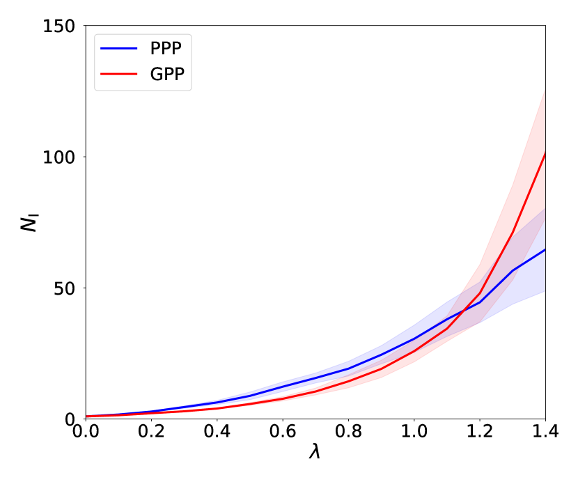
Figure 9: For the SIR model with (9) the quenched averages $\langle\mathcal{N}_{\mathrm{I}}\rangle$ of the cumulative numbers of infected individuals (11) are shown versus $\lambda$ for the PPP-based model by a blue curve and for the GPP-based model by a red curve. The standard deviations in the ten samples are shown by shaded strips around the curves. We find a crossing point of these two curves at $\lambda_{*}\simeq 1.2$.

We thought that the difference between $\langle\mathcal{N}_{\mathrm{I}}^{\rm PPP}\rangle$ and $\langle\mathcal{N}_{\mathrm{I}}^{\rm GPP}\rangle$ can be simply attribute to the difference in the distributions of degree shown by Fig. 2 in Section 1. In order to verify this naive conjecture, we considered the following modifications of (9),

$$\Psi_{\leq 1}(n) =1,\quad\forall n\geq 1,$$

$$\Psi_{\leq 2}(n) =\begin{cases}n,&\quad(n=1,2),\cr 1,&\quad(n\geq 3),\end{cases}$$

$$\Psi_{\leq 4}(n) =\begin{cases}n,&\quad(n=1,2,3,4),\cr 1,&\quad(n\geq 5),\end{cases}$$

$$\Psi_{\geq 5}(n) =\begin{cases}1,&\quad(n=1,2,3,4),\cr n,&\quad(n\geq 5).\end{cases}$$

The ratios $\langle\mathcal{N}_{\mathrm{I}}^{\rm GPP}\rangle/\langle\mathcal{N}_{\mathrm{I}}^{\rm PPP}\rangle$ are plotted versus $\lambda$ in Fig. 10 for these different models as well as for the original linear model (9) and for the quadratic model with $\widehat{\Psi}(n)=n^{2}$. We found the similarities between the models with $\Psi_{\leq 1}$ and with $\Psi_{\geq 5}$, and between the model with $\Psi_{\leq 4}$ and the original linear model (9). These observations imply that the cases with $n\geq 5$ do not contribute to the present phenomenon. So we reconsidered the original linear model more carefully.

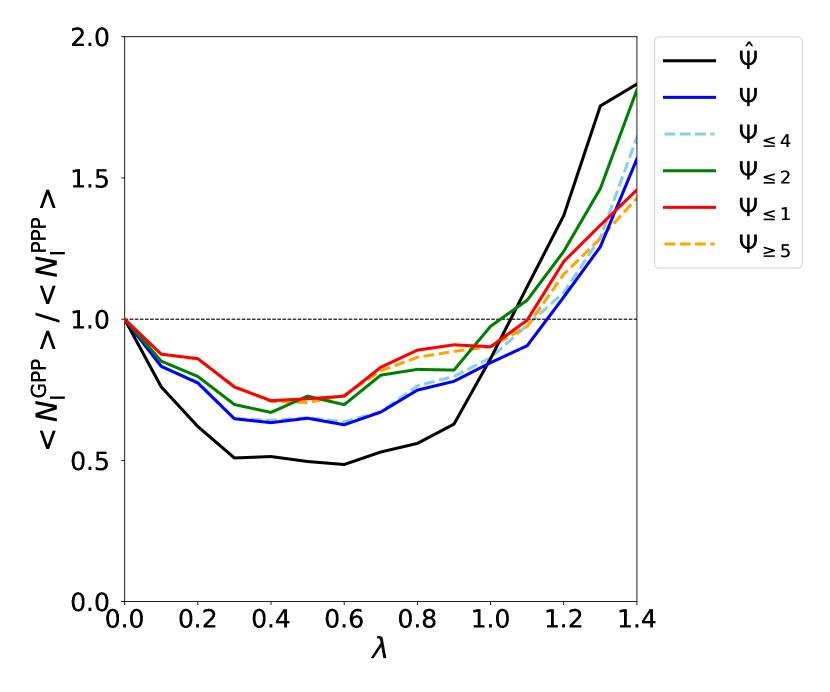
Figure 10: Ratios $\langle\mathcal{N}^{\rm GPP}_{\mathrm{I}}\rangle/\langle\mathcal{N}^{\rm PPP}_{\mathrm{I}}\rangle$ are plotted versus $\lambda$ for several models with different choices of $\Psi$.

In each realization of process, we traced a time-sequence of points at each of which a transition $\mathrm{S}\to\mathrm{I}$ was taken place, and counted the number of infected individuals in the neighborhood of each point. We obtained the distribution of the number of infected neighbors $n$ using the data of 100 runs on each underlying graph $\mathcal{G}$, and then we calculated the quenched average of distributions over ten samples of $\mathcal{G}$. Figure 11 shows the distributions of $n$ when $\lambda=0.5$ for the PPP-based and the GPP-based models.

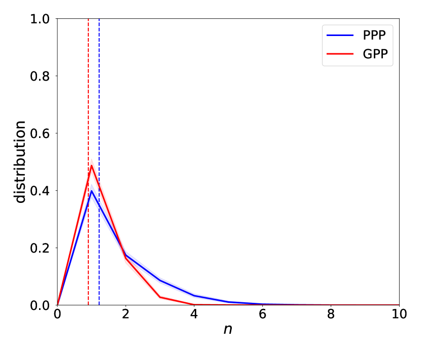
Figure 11: Distributions of $n$ are shown for the PPP-based and the GPP-based SIR model with (9), when $\lambda=0.5$. Solid lines show the quenched averages of ten distinct samples of $\mathcal{G}$ and shaded strips show the standard deviations of them. The means of $n$ in the PPP-based model and the GPP-based model are 1.22 and 0.904, respectively.

Compared with the distributions of degree in underlying graphs shown by Fig. 2, any contribution from hubs with a large number of neighbors [9] are truncated in the ‘effective network’ for the present SIR models. The difference of distributions of $n$ between the PPP-based model and the GPP-based model seems to be very small in Fig. 11, but this difference definitely causes the discrepancy between the curve for the model with $\Psi_{\leq 1}$ (to which the curve for the model with $\Psi_{\geq 5}$ is similar) and that with the original linear function (9) (to which the curve with $\Psi_{\leq 4}$ is similar) shown in Fig. 10. We should notice that even in the model with $\Psi_{\leq 1}$, which has no dependence on $n\geq 1$, Fig. 10 shows the suppression $\langle\mathcal{N}_{\mathrm{I}}^{\rm GPP}\rangle/\langle\mathcal{N}_{\mathrm{I}}^{\rm PPP}\rangle<1$ for $\lambda<\lambda_{*}$. This effect will be attributed to blobs in underlying percolation cluster $\mathcal{G}$ [37]. A blob is constructed on clumping of points in the PPP caused by the Poissonian large fluctuation. And it is observed as an infection cluster which seems to be compact but included relatively large number of infected individuals. The comparison to the GPP-based model was already demonstrated by Fig. 4 in Section 1.

As shown by Fig. 3 and Fig. 10, the suppression of infection clusters in the GPP-based model is much enhanced, when the contagion is described by the ‘quadratic SIR model’ with $\widehat{\Psi}(n)=n^{2}$, $n\in\mathbb{N}$.

5 Concluding Remarks

Among a variety of continuum percolation models (see, for instance, Chapter 8 of [29] and Chapter 8 of [30]) we have focused on the Boolean model with same-radius disks (the standard Gilbert disk model [28]) on $\mathbb{R}^{2}$ in this paper. Even in this simplest model, many works have been done in the case that the model is driven by the uniform PPP. On the other hand, the GPP and other determinantal point processes (DPPs) have been extensively studied in random matrix theory [18, 19, 25] and the hyperuniformity of such repelling point processes has attracted much attention in many research fields [26, 27]. Recently comparison of clustering properties between the PPP and non-Poisson point processes is mathematically studied [31, 32]. The continuum percolation models driven by DPPs are also studied in probability theory [33]. In the present paper we reported a numerical study on the Boolean percolation models defined on the PPP and the GPP. The purpose of the comparison between these two kinds of continuum percolation models here is to construct the SIR models of infection processes on them and to clarify differences in stochastic properties of infection clusters between the PPP-based and the GPP-based models. We are interested in hierarchical modeling such that the underlying graph $\mathcal{G}$ is formed using a random point process and a notion of continuum percolation, and then a time-dependent system is constructed on $\mathcal{G}$.

We list out remarks on open problems and future directions.

1. We reported the numerical evaluation of the critical filling factor $\kappa_{\rm c}^{\rm GPP}$ for the Boolean percolation model on $\mathbb{R}^{2}$ defined on the GPP. We can find a series of papers on numerical evaluations of $\kappa_{\rm c}^{\rm PPP}$; see [42, 43, 45, 38] and references therein. Further study on more precise enumeration of $\kappa_{\rm c}^{\rm GPP}$ should be done.

2. Our estimations of the critical infection rates $\lambda_{\rm c}^{\rm PPP}(\kappa)$ and $\lambda_{\rm c}^{\rm GPP}(\kappa)$ of the SIR models are preliminary and they are given only for a special value $\kappa=1.3$ of the filling factor in the underlying Boolean percolation models. Since we have been interested in infection processes with $\lambda$ which is much smaller than $\lambda_{\rm c}$ in the present work, we did not need precise values of $\lambda_{\rm c}$. Systematic study on the critical value $\lambda_{\rm c}(\kappa)$ as a function of $\kappa$ as well as on the critical phenomena [10, 41, 48, 49, 11, 12, 15] observed in the vicinity of the critical line $\lambda=\lambda_{\rm c}(\kappa)$, $\kappa>0$ is required [47].

3. The present numerical results show the strict inequalities $\kappa_{\rm c}^{\rm GPP}<\kappa_{\rm c}^{\rm PPP}$ and $\lambda_{\rm c}^{\rm GPP}<\lambda_{\rm c}^{\rm PPP}$. They suggest that covering processes and spreading phenomena can be achieved more efficiently in the GPP-based models than the PPP-based models. We find interesting examples of this fact in the work on modeling and analysis of cellular networks [50, 51, 52]. In the present paper, however, we have reported an opposite tendency such that emergence of infection clusters in contagious processes is suppressed in the GPP-based model compared to the PPP-based model, if the infectivity $\lambda$ is less than a special value denoted by $\lambda_{*}$. We are planning to proceed the study reported in Section 4.3 in order to understand the mechanism determining the values of $\lambda_{*}$. Moreover, effect of nonlinearity of the function $\Psi(n),n\in\mathbb{N}$ on this phenomenon should be clarified in the future study [47].

4. As well-defined random point processes with positive correlations, permanental (Boson) point processes have been studied in probability theory [21, 22, 53, 54, 24, 55]. Infection models on permanental point processes shall be studied and compared with the present SIR models on the Poisson point process and the Ginibre point process.

CRediT authorship contribution statement

Machiko Katori: Conceptualization, Methodology, Analytical results, Numerical results, Writing. Makoto Katori: Conceptualization, Methodology, Writing.

References

- [1] W. O. Kermack, A. G. McKendrick, A contribution to the mathematical theory of epidemics, Proc. R. Soc. London. Ser. A, Contain. Pap. a Math. Phys. Character 115 (772) (1927) 700–721. doi:10.1098/rspa.1927.0118.
- [2] N. T. J. Bailey, The total size of a general stochastic epidemic, Biometrika 40 (1/2) (1953) 177. doi:10.2307/2333107.
- [3] N. T. J. Bailey, The Mathematical Theory of Epidemics, Hafner, New York, 1957.
- [4] T. M. Liggett, Interacting Particle Systems, Classics in Mathematics, Springer, Berlin, Heidelberg, 1985. doi:10.1007/b138374.
- [5] R. M. Anderson, R. M. May, Infectious Diseases of Humans: Dynamics and Control., Oxford University Press, Oxford, UK, 1991.
- [6] T. M. Liggett, Stochastic Interacting Systems: Contact, Voter and Exclusion Processes, Vol. 324 of Grundlehren der mathematischen Wissenschaften, Springer, Berlin, Heidelberg, 1999. doi:10.1007/978-3-662-03990-8.
- [7] O. Diekmann, J. A. P. Heesterbeek, Mathematical Epidemiology of Infectious Diseases: Model Building, Analysis and Interpretation, John Wiley and Sons, Chichester, 2000.
- [8] G. Chowell, J. M. Hyman, L. M. A. Bettencourt, C. Castillo-Chavez (Eds.), Mathematical and Statistical Estimation Approaches in Epidemiology, Springer Netherlands, Dordrecht, 2009. doi:10.1007/978-90-481-2313-1.
- [9] A.-L. Barabási, Network Science, Cambridge University Press, Cambridge, 2016.
- [10] P. Grassberger, On the critical behavior of the general epidemic process and dynamical percolation, Math. Biosci. 63 (2) (1983) 157–172. doi:10.1016/0025-5564(82)90036-0.
- [11] D. R. de Souza, T. Tomé, Stochastic lattice gas model describing the dynamics of the SIRS epidemic process, Phys. A Stat. Mech. its Appl. 389 (5) (2010) 1142–1150. doi:10.1016/j.physa.2009.10.039.
- [12] T. Tomé, R. M. Ziff, Critical behavior of the susceptible-infected-recovered model on a square lattice, Phys. Rev. E 82 (5) (2010) 051921. doi:10.1103/PhysRevE.82.051921.
- [13] S. Saha, A. Mishra, S. K. Dana, C. Hens, N. Bairagi, Infection spreading and recovery in a square lattice, Phys. Rev. E 102 (5) (2020) 052307. doi:10.1103/PhysRevE.102.052307.
- [14] G. Santos, T. Alves, G. Alves, A. Macedo-Filho, R. Ferreira, Epidemic outbreaks on two-dimensional quasiperiodic lattices, Phys. Lett. A 384 (2) (2020) 126063. doi:10.1016/j.physleta.2019.126063.
- [15] R. M. Ziff, Percolation and the pandemic, Phys. A Stat. Mech. its Appl. 568 (2021) 125723. doi:10.1016/j.physa.2020.125723.
- [16] D. Daley, D. Vere-Jones, An Introduction to the Theory of Point Processes, 2nd Edition, Probability and its Applications, Springer-Verlag, New York, 2003. doi:10.1007/b97277.
- [17] J. Ginibre, Statistical ensembles of complex, quaternion, and real matrices, J. Math. Phys. 6 (3) (1965) 440–449. doi:10.1063/1.1704292.
- [18] M. L. Mehta, Random Matrices, 3rd Edition, Elsevier, Amsterdam, 2004. doi:10.1016/C2009-0-22297-5.
- [19] P. J. Forrester, Log-Gases and Random Matrices, Princeton University Press, Princeton, 2010. doi:10.1515/9781400835416.
- [20] A. Soshnikov, Determinantal random point fields, Russ. Math. Surv. 55 (5) (2000) 923–975. doi:10.1070/RM2000v055n05ABEH000321.
- [21] T. Shirai, Y. Takahashi, Random point fields associated with certain Fredholm determinants I: fermion, Poisson and boson point processes, J. Funct. Anal. 205 (2) (2003) 414–463. doi:10.1016/S0022-1236(03)00171-X.
- [22] T. Shirai, Y. Takahashi, Random point fields associated with certain Fredholm determinants II: fermion shifts and their ergodic and Gibbs properties, Ann. Probab. 31 (3) (2003) 1533–1564. doi:10.1214/aop/1055425789.
- [23] T. Shirai, Large deviations for the fermion point process associated with the exponential kernel, J. Stat. Phys. 123 (3) (2006) 615–629. doi:10.1007/s10955-006-9026-x.
- [24] J. Hough, M. Krishnapur, Y. Peres, B. Virág, Zeros of Gaussian Analytic Functions and Determinantal Point Processes, Vol. 51 of University Lecture Series, American Mathematical Society, Providence, Rhode Island, 2009. doi:10.1090/ulect/051.
- [25] M. Katori, Bessel Processes, Schramm–Loewner Evolution, and the Dyson Model, Vol. 11 of SpringerBriefs in Mathematical Physics, Springer, Singapore, 2016. doi:10.1007/978-981-10-0275-5.
- [26] S. Torquato, Hyperuniform states of matter, Phys. Rep. 745 (2018) 1–95. doi:10.1016/j.physrep.2018.03.001.
- [27] T. Matsui, M. Katori, T. Shirai, Local number variances and hyperuniformity of the Heisenberg family of determinantal point processes, J. Phys. A Math. Theor. 54 (16) (2021) 165201. doi:10.1088/1751-8121/abecaa.
- [28] E. N. Gilbert, Random plane networks, J. Soc. Ind. Appl. Math. 9 (4) (1961) 533–543.
- [29] R. Meester, R. Roy, Continuum Percolation, Cambridge Tracts in Mathematics, Cambridge University Press, Cambridge, 1996. doi:10.1017/CBO9780511895357.
- [30] B. Bollobas, O. Riordan, Percolation, Cambridge University Press, Cambridge, 2006. doi:10.1017/CBO9781139167383.
- [31] B. Błaszczyszyn, D. Yogeshwaran, Clustering and percolation of point processes, Electron. J. Probab. 18 (72) (2013) 1. doi:10.1214/EJP.v18-2468.
- [32] B. Błaszczyszyn, D. Yogeshwaran, On comparison of clustering properties of point processes, Adv. Appl. Probab. 46 (1) (2014) 1–20. doi:10.1239/aap/1396360100.
- [33] S. Ghosh, M. Krishnapur, Y. Peres, Continuum percolation for Gaussian zeroes and Ginibre eigenvalues, Ann. Probab. 44 (5) (2016) 3357–3384. doi:10.1214/15-AOP1051.
- [34] D. T. Gillespie, A general method for numerically simulating the stochastic time evolution of coupled chemical reactions, J. Comput. Phys. 22 (4) (1976) 403–434. doi:10.1016/0021-9991(76)90041-3.
- [35] D. T. Gillespie, Exact stochastic simulation of coupled chemical reactions, J. Phys. Chem. 81 (25) (1977) 2340–2361. doi:10.1021/j100540a008.
- [36] R. Erban, S. J. Chapman, Stochastic Modelling of Reaction–Diffusion Processes, Cambridge Texts in Applied Mathematics, Cambridge University Press, 2020. doi:10.1017/9781108628389.
- [37] D. Stauffer, A. Aharony, Introduction to Percolation Theory, Taylor & Francis, London, 1992. doi:10.1201/9781315274386.
- [38] S. Mertens, C. Moore, Continuum percolation thresholds in two dimensions, Phys. Rev. E 86 (6) (2012) 061109. doi:10.1103/PhysRevE.86.061109.
- [39] E. T. Gawlinski, H. E. Stanley, Continuum percolation in two dimensions: Monte Carlo tests of scaling and universality for non-interacting discs, J. Phys. A. Math. Gen. 14 (8) (1981) L291–L299. doi:10.1088/0305-4470/14/8/007.
- [40] I. Balberg, N. Binenbaum, C. H. Anderson, Critical behavior of the two-dimensional sticks system, Phys. Rev. Lett. 51 (18) (1983) 1605–1608. doi:10.1103/PhysRevLett.51.1605.
- [41] J. L. Cardy, P. Grassberger, Epidemic models and percolation, J. Phys. A. Math. Gen. 18 (6) (1985) L267–L271. doi:10.1088/0305-4470/18/6/001.
- [42] J. Quintanilla, S. Torquato, Percolation for a model of statistically inhomogeneous random media, J. Chem. Phys. 111 (13) (1999) 5947–5954. doi:10.1063/1.479890.
- [43] J. Quintanilla, S. Torquato, R. M. Ziff, Efficient measurement of the percolation threshold for fully penetrable discs, J. Phys. A. Math. Gen. 33 (42) (2000) L399–L407. doi:10.1088/0305-4470/33/42/104.
- [44] M. E. J. Newman, R. M. Ziff, Fast Monte Carlo algorithm for site or bond percolation, Phys. Rev. E 64 (1) (2001) 016706. doi:10.1103/PhysRevE.64.016706.
- [45] J. A. Quintanilla, R. M. Ziff, Asymmetry in the percolation thresholds of fully penetrable disks with two different radii, Phys. Rev. E 76 (5) (2007) 051115. doi:10.1103/PhysRevE.76.051115.
- [46] A. B. Bortz, M. H. Kalos, J. L. Lebowitz, A new algorithm for Monte Carlo simulation of Ising spin systems, J. Comput. Phys. 17 (1) (1975) 10–18. doi:10.1016/0021-9991(75)90060-1.
- [47] Machiko Katori, Makoto Katori, Spreading and suppression of infection clusters on the Ginibre continuum percolation clusters, arXiv (2021). arXiv:2105.04142.
- [48] H. Hinrichsen, Non-equilibrium critical phenomena and phase transitions into absorbing states, Adv. Phys. 49 (7) (2000) 815–958. doi:10.1080/00018730050198152.
- [49] T. Vojta, A. Farquhar, J. Mast, Infinite-randomness critical point in the two-dimensional disordered contact process, Phys. Rev. E 79 (1) (2009) 011111. doi:10.1103/PhysRevE.79.011111.
- [50] N. Miyoshi, T. Shirai, A cellular network model with Ginibre configured base stations, Adv. Appl. Probab. 46 (3) (2014) 832–845. doi:10.1239/aap/1409319562.
- [51] Y. Li, F. Baccelli, H. S. Dhillon, J. G. Andrews, Statistical modeling and probabilistic analysis of cellular networks with determinantal point processes, IEEE Trans. Commun. 63 (9) (2015) 3405–3422. doi:10.1109/TCOMM.2015.2456016.
- [52] N. Miyoshi, T. Shirai, Spatial modeling and analysis of cellular networks using the Ginibre point process: A tutorial, IEICE Trans. Commun. E99.B (11) (2016) 2247–2255. doi:10.1587/transcom.2016NEI0001.
- [53] H. Tamura, K. R. Ito, A canonical ensemble approach to the fermion/boson random point processes and its applications, Commun. Math. Phys. 263 (2) (2006) 353–380. doi:10.1007/s00220-005-1507-2.
- [54] H. Tamura, K. R. Ito, A random point field related to Bose–Einstein condensation, J. Funct. Anal. 243 (1) (2007) 207–231. doi:10.1016/j.jfa.2006.10.014.
- [55] I. Armendáriz, P. A. Ferrari, S. Yuhjtman, Gaussian random permutation and the boson point process, arXiv (2019). arXiv:1906.11120.