Asymptotic absorption-time distributions in extinction-prone Markov processes

Abstract

We characterize absorption-time distributions for birth-death Markov chains with an absorbing boundary. For “extinction-prone” chains (which drift on average toward the absorbing state) the asymptotic distribution is Gaussian, Gumbel, or belongs to a family of skewed distributions. The latter two cases arise when the dynamics slow down dramatically near the boundary. Several models of evolution, epidemics, and chemical reactions fall into these classes; in each case we establish new results for the absorption-time distribution. Applications to African sleeping sickness are discussed.

Modeling extinction-prone dynamics is essential to our understanding of epidemics, disease incubation, and evolution. For example, a key goal in epidemiology is to implement control measures (such as social distancing or vaccination) that push the dynamics toward a state where the disease is eradicated on a reasonable timescale [1, 2, 3]. Similarly, disease incubation [4, 5] and evolution [6, 7] involve highly fit infectious cells or mutant species outcompeting their less fit counterparts.

In these fields the distribution of extinction times, rather than just the mean, is crucial. For example, how long must a patient wait after exposure to a disease to be sure they are not infected? In the best and worst case scenarios, how long must epidemiological control measures be imposed to stop an outbreak? Knowledge of the extinction-time distribution provides an answer to these questions. Incubation period distributions have long been measured empirically to inform treatment regimens or public health initiatives [4]. Similarly, a recent study used a data-driven model of African sleeping sickness in the Democratic Republic of Congo to predict the distribution of times until the disease is eradicated [3].

In this Letter, we show that two particular extinction-time distributions—Gaussian and Gumbel distributions—arise generically from basic features of the stochastic dynamics driving the system. These distributions were found previously in several models of evolutionary dynamics [5, 8, 9]. We show now that these same distributions appear in much more general classes of birth-death Markov chains, along with a family of skewed distributions that include the Gumbel. Extending the approach introduced in Ref. [9], we provide analytical criteria that predict when the asymptotic absorption-time distribution is normal, Gumbel, or a member of the family of skewed distributions. We apply our results to models of epidemiology [10, 11, 12], ecology [13, 14, 15], stochastic chemical reactions [16, 17], and evolutionary games [18], for which the predicted distributions agree with those measured via simulation. To our knowledge, this is the first calculation of the asymptotic absorption-time distributions for these models. As an application, we show that the Gumbel distribution closely resembles eradication-time distributions for African sleeping sickness.

We analyze birth-death Markov processes with a linear chain of states $m=0,1,\dots,N$. For example, $m$ might represent the number of infected individuals in an epidemic. The system has an absorbing state at $m=0$ (where nobody is infected) and a reflecting state at $m=N$ (the maximum allowed infected population). Transitions occur only between neighboring states, i.e., the population can only increment by 1 in either direction. The dynamics of $p_{m}(t)$, the probability of occupying state $m$ at time $t$, obey the master equation,

$$\dot{p}_{m}(t)=b_{m-1}p_{m-1}(t)+d_{m+1}p_{m+1}(t)-(b_{m}+d_{m})p_{m}(t),$$ (1)

where $b_{m}$ and $d_{m}$ are respectively the birth and death rates at which the state increases or decreases from state $m$. The master equation can also be expressed as $\dot{\mathbf{p}}(t)=\Omega\cdot\mathbf{p}(t)$, where $\Omega$ is the transition matrix containing the birth and death rates. Since the state at $m=0$ is absorbing and the state $m=N$ is reflecting, we have $b_{0}=b_{N}=0$. For simplicity we assume the system starts in an initial state $m=N$, i.e. $p_{m}(0)=\delta_{m,N}$, but our results apply more broadly [19]. The quantity we are interested in is the first-passage time $T$ to the absorbing state $m=0$; here we focus on obtaining the probability distribution about the mean.

Building on our recent results [9], we develop an approach to determine the absorption-time distributions for general classes of birth-death Markov chains in the limit of large system size. The key insight is to introduce a change of variables, $D_{m}=b_{m}+d_{m}$ and $r_{m}=b_{m}/d_{m}$. If the system is in state $m$, it waits on average a time $D_{m}^{-1}$ before increasing or decreasing. The probabilities of the next step being forward or backward are $r_{m}/(1+r_{m})$ and $1/(1+r_{m})$ respectively; $r_{m}$ is the ratio of these probabilities. Thus, our coordinate change separates the random-walk portion of the Markov process, which describes the relative probabilities of stepping forward or backward at each state, from the times spent waiting in each state. This change of variables leads to a transition matrix decomposition, $\Omega=\Omega_{RW}D$, where $D$ is diagonal with elements $D_{m}$ and $\Omega_{RW}$ is the transition matrix for a biased random walk. The number of times the system visits each state depends only on the random-walk portion of the process. The elements $V_{ij}$ of $V=-\Omega_{RW}^{-1}$ encode the average number of visits to state $i$ before absorption, starting from state $j$.

To characterize the asymptotic distributions, we compute the cumulants $\kappa_{n}(N)$ of the absorption time $T$, which describe the shape of the distribution. For instance, $\kappa_{1}$ is the mean, $\kappa_{2}$ is the variance, and $\kappa_{3}/\kappa_{2}^{3/2}$ is the skew. Following Ref. [9] we use the matrix decomposition above to derive the cumulants (generalizing the previous result to non-constant $r_{j}$):

$$\color[rgb]{0,0,0}\kappa_{n}(\{r_{j}\},N)=\sum_{1\leq i_{1}\leq i_{2}\leq\dots\leq i_{n}\leq N}\frac{w_{i_{1}i_{2}\cdots i_{n}}^{n}(\{r_{j}\})}{(b_{i_{1}}+d_{i_{1}})\cdots(b_{i_{n}}+d_{i_{n}})}.$$ (2)

Here $w_{i_{1}i_{2}\cdots i_{n}}^{n}(\{r_{j}\})$ are weighting factors that depend only on the visit statistics of the random walk; for example, $w_{i}^{1}(\{r_{j}\})=V_{i,i}$. See the Supplemental Material [19] for a derivation of this formula and explicit expressions for the first few weighting factors, each of which are polynomials of the visit numbers $V_{ij}$. Equation (2) is equivalent to well known recursive relations for absorption time moments [20], but this form enables the asymptotic analysis leading to the results below.

The weighting factors have some convenient properties. First, they appear to be non-negative: $w_{i_{1}i_{2}\cdots i_{n}}^{n}(\{r_{j}\})\geq 0$ and increasing functions of each $r_{j}$. We show the non-negativity and monotonicity explicitly up to order $n=4$ [19] and conjecture these properties hold for all orders. Second, the weighting factors appear to fall off exponentially away from the diagonal. For constant $r_{j}=r$, this exponential decay can be shown explicitly [9]. We conjecture that the same decay holds for arbitrary transition probabilities $\{r_{j}\}$. The intuition is that the visits to state $i$ are uncorrelated with those to state $j$ (for $N\gg 1$ and $i-j=\mathcal{O}(N)$), due to the Markov property.

The first universality class of birth-death Markov chains we consider have normally distributed absorption times. As an instructive special case, consider the process $b_{m}=0$, $d_{m}=d$, which visits each state exactly once before absorption, waiting a time $d^{-1}$ on average at each. The time to absorption is simply $T=\sum_{m}\mathcal{E}_{m}(d)$ where $\mathcal{E}_{m}(d)$ is an exponential random variable. Since $T$ is a sum of identical random variables we expect it to be normally distributed by the central limit theorem. Alternatively, the cumulants of $T$ are $\kappa_{n}=N/d^{n}$. In units of the standard deviation the higher order cumulants vanish: $\kappa_{n}/\kappa_{2}^{n/2}=N^{1-n/2}\to 0$ as $N\rightarrow\infty$. Hence the distribution is asymptotically normal.

We might also expect this asymptotic normality to hold for transition rates with mild state dependence: if $b_{m}+d_{m}$ does not vary too much (we will give a precise condition below), the absorption time is a sum of nearly identical exponential random times. Similarly, for $r_{m}=b_{m}/d_{m}>0$, the system randomly walks back and forth, but as long as $r_{m}<1$ the average number of visits to each state is finite. Under either of these generalizations the distribution is asymptotically normal.

To characterize more precisely which Markov chains lead to normally distributed absorption times, we compute the asymptotic form of the cumulants in Eq. (2) by introducing two auxiliary Markov chains. These have the same $b_{i}+d_{i}$ as the original system, but $b_{i}$ and $d_{i}$ are adjusted so that the ratios are $r_{j}=r_{\max}$ or $r_{j}=r_{\min}$, where $r_{\max}=\lim_{N\rightarrow\infty}\max_{1<j<N}r_{j}$ and $r_{\min}=\lim_{N\rightarrow\infty}\min_{1<j<N}r_{j}$. In other words, we construct two Markov chains where the time spent waiting in each state is identical to that for the original system, but the odds of moving toward the absorbing state are increased or decreased to be uniform.

Above we noted that the weighting factors $w^{n}$ in Eq. (2) are increasing functions of $r_{j}$. Thus, we can bound the cumulants in our system by those for the auxiliary Markov chains, $\kappa_{n}(r_{\min},N)\leq\kappa_{n}(\{r_{j}\},N)\leq\kappa_{n}(r_{\max},N)$. The asymptotic form of $\kappa_{n}(r,N)$ (where $r$ is constant across states) was computed in Ref. [9]; we summarize the calculation in the Supplemental Material [19]. To nail down the asymptotics of $\kappa_{n}(r,N)$ we require the waiting times to be ‘flat’ in the following sense:

$$\color[rgb]{0,0,0}\frac{1}{N}\sum_{m=1}^{N}t_{m}\sim c\max_{1\leq m\leq N}t_{m},$$ (3)

where $t_{m}=(b_{m}+d_{m})^{-1}$ is the mean waiting time at state $m$ and $c$ is a constant independent of $N$. In other words, the mean waiting time $\langle t_{m}\rangle$ across all states is the same asymptotic order as the maximum waiting time: the process fluctuates at an approximately uniform rate across the entire Markov chain, without spending a disproportionate amount of time in any one state. Gaussian absorption times have also been found in the continuum limit via the linear-noise approximation, which removes state dependence from the noise [21]. This approximation is similar to the condition (3), which requires the noise amplitude $b_{m}+d_{m}$ to vary only mildly across states.

If Eq. (3) holds, then $\kappa_{n}(r,N)\sim c_{n}(r)f(N)^{n}N$, where $f(N)\sim\max_{1\leq i\leq N}(b_{i}+d_{i})^{-1}$. Since these asymptotics hold for $r=r_{\min}$ and $r=r_{\max}$, it follows that $\kappa_{n}(\{r_{j}\},N)\sim c_{n}(\{r_{j}\})f(N)^{n}N$ as well.

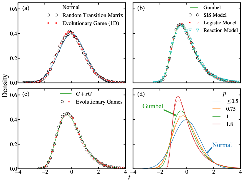
Figure 1: Absorption-time distributions for (a) the random transition matrix model (large black circles) and the evolutionary game on a ring (small red circles), (b) SIS model (large black circles), logistic model (small red circles), and autocatalytic chemical reaction model (cyan triangles), (c) the well-mixed evolutionary game, and (d) the process $b_{m}=rd_{m}=rm^{p}$, for $r=0$ and $p=0.3$ (blue), $p=0.75$ (orange), $p=1$ (green), and $p=1.8$ (red). The $r=0.8$ distributions are indicated by dotted lines (when they differ from the $r=0$ counterparts). See [19] for models and parameters. We used system sizes (a-b) $N=500$ and (c-d) $N=1000$ and simulated (a) $5\times 10^{4}$, (b-c) $10^{5}$, and (d) $10^{6}$ trials to measure the distributions, which have been standardized to have zero mean and unit variance. In (c) the distributions are a convolution of Gumbel distributions with relative weighting $s\approx 0.73$. Deviations from predicted normal and Gumbel distributions in (a-c) are due to finite system size.

With the asymptotic form of the cumulants established, we analyze the shape of the distribution using the standardized cumulants $\tilde{\kappa}_{n}=\kappa_{n}/\kappa_{2}^{n/2}$ for $n\geq 2$ (which are rescaled so that the variance $\tilde{\kappa}_{2}=1$). Using the asymptotic form obtained above, we find $\tilde{\kappa}_{n}\sim\tilde{c}_{n}N^{1-n/2}$. In particular, $\tilde{\kappa}_{n}\rightarrow 0$ as $N\rightarrow\infty$ for $n>2$, so that the distribution becomes Gaussian for large $N$ (the cumulants past second order vanish for normal distributions).

For finite $N$, the dominant correction to the normal distribution comes from the non-zero skew $\tilde{\kappa}_{3}\sim\tilde{c}_{3}/\sqrt{N}$. The coefficient in this scaling depends on the ratios $r_{j}$; in the Supplemental Material [19] we compute a bound on this coefficient, which is useful for estimating the rate of convergence in applications. The ratio of the standard deviation $\kappa_{2}^{1/2}$ to the mean $\kappa_{1}$ also scales like $\kappa_{2}^{1/2}/\kappa_{1}\sim\tilde{c}_{1}/\sqrt{N}$, similar to the skew. As the distribution converges to the Gaussian, the relative width of the distribution narrows at the same rate. To summarize, any birth-death Markov chain that satisfies the ‘flatness’ condition, Eq. (3), and has an absorbing state toward which the system flows on average ($r_{j}<1$) will have asymptotically Gaussian distributed absorption times.

Our first example of a Markov chain with normally distributed absorption times is a toy model with random transition probabilities. Here we select $b_{m}+d_{m}$ uniformly at random between 0.1 and 2 and $r_{m}$ uniformly at random between $0$ and $0.9$, which satisfies the conditions described above. This example shows that the transition rates need not be smooth in $m$; systems with disordered transition rates still belong to this universality class.

Next we study evolutionary game dynamics on a one-dimensional ring [22, 23]. Mutant and wild-type individuals compete via the following dynamics: an individual is chosen randomly, proportional to its (frequency dependent) fitness. The selected individual gives birth to an offspring of the same type, which in turn replaces a random neighbor. The model runs until the mutation spreads to the entire population.

Figure 1(a) shows simulation results for the random transition system and the evolutionary game. Both display the expected normal distribution. Interestingly, for the evolutionary game, the normal distribution appears for a wide range of parameters, while the mean absorption time and absorption probability depend more intricately on parameters [22, 23].

Gumbel distributions, known for their role in extreme value theory [24], also arise generically in absorption processes. This second universality class is closely related to the ‘coupon collector’ problem in probability theory, which asks the following: if there are $N$ distinct coupons and we are given a random one (with replacement) at each time step, how long does it take to collect all $N$ coupons? The collection process displays a characteristic slowdown: when nearly all coupons have been collected, it takes a long time to acquire the final few because duplicates keep getting selected. Erdős and Rényi showed that for large $N$ the time to complete the collection follows a Gumbel distribution [25].

The coupon collector problem can be modeled using Markov chains. Let $m$ be the number of coupons missing from the collection of $N$ total coupons. The probability of obtaining a new coupon (thereby decreasing $m$) is $m/N$ and the number of missing coupons never increases. Thus, the coupon collection process is described by birth-death dynamics with $b_{m}=0$ and $d_{m}=m/N$. The linear decay of the transition probability $d_{m}$ near the absorbing boundary is the key feature that gives rise to the characteristic slowdown. For this case the cumulants can be computed exactly, $\tilde{\kappa}_{n}=(n-1)!\zeta(n)/\zeta(2n)^{n/2}$, and match those for a Gumbel distribution. Similar to the Gaussian class above, we find that the Gumbel distribution is preserved for non-zero $r_{m}<1$ and nonlinear transition rates as long as the linear decay is dominant near $0$. Specifically, if $b_{m}+d_{m}=f(N)m[1+\mathcal{O}(m/N)]$, with $b_{\alpha N}+d_{\alpha N}$ of order at least $\mathcal{O}(Nf(N))$ for any $0<\alpha\leq 1$, and if $r_{m}=r+\mathcal{O}(m/N)$ for large $N$, then the absorption-time distribution is asymptotically Gumbel .

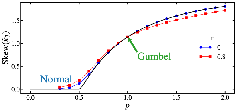
Figure 2: Absorption-time skew for the process $b_{m}=rd_{m}=rm^{p}$ with $r=0$ (blue circles) and $r=0.8$ (red squares), plotted as a function of the power-law exponent $p$. Skews were numerically computed for $N=10^{5}$ using the recurrence relation approach described in Ref. [9]. The black line shows the asymptotic skew $2\zeta(3p)/\zeta(2p)^{3/2}$ for $r=0$. The curves cross at $p=1$ where the distribution is Gumbel, independent of $r$. For $p\leq 0.5$ the skew approaches zero and the distribution is Gaussian. The numerical skew is slightly larger than expected for $p\lesssim 0.6$ due to finite size effects.

By bounding the cumulants (2), we show [19] their leading order behavior for $N\gg 1$ is dominated by the states near 0, where the approximations $b_{m}+d_{m}\approx f(N)m$ and $r_{m}\approx r$ become asymptotically exact, so that

$$\kappa_{n}(\{r_{j}\},N)\sim\frac{1}{f(N)^{n}}\sum_{1\leq i_{1}\leq i_{2}\leq\dots\leq i_{n}\leq N}\frac{w_{i_{1}i_{2}\cdots i_{n}}^{n}(r)}{i_{1}i_{2}\cdots i_{n}}.$$ (4)

The factors $f(N)^{n}$ set the timescale of the process but do not affect the shape of the distribution (they cancel in $\tilde{\kappa}_{n}=\kappa_{n}/\kappa_{2}^{n/2}$). Thus, we have shown that the cumulants are asymptotic to those for a process with $b_{m}+d_{m}=m$ and $b_{m}/d_{m}=r$. The absorption-time distribution for this process can be computed exactly (see Ref. [14, Appendix B]) and approaches a Gumbel distribution as $N\to\infty$ [19]. Therefore, any system with transition rates vanishing linearly and ratios $r_{j}$ that approach a constant near the absorbing boundary will fall into the Gumbel universality class.

As in the Gaussian class, the relative width of the Gumbel distributions becomes small for $N\gg 1$. In this case, however, the standard deviation-to-mean ratio scales like $\kappa_{2}^{1/2}/\kappa_{1}\sim C_{1}/\ln N$. On the other hand, the deviations from the Gumbel cumulants decay like $\delta\tilde{\kappa}_{n}=\tilde{\kappa}_{n}-\tilde{\kappa}_{n}^{\mathrm{Gumbel}}\sim C_{n}N^{-1}\ln N$ (see Supplemental Material, Section S3.A [19] and [26]). Thus the distribution narrows very slowly compared to the convergence to the Gumbel shape. Therefore, in applications we expect to see the Gumbel distribution appear before the fluctuations become negligible.

Finally, if the transition rates vanish near the initial condition $N$, scaling like $b_{m}+d_{m}=\tilde{f}(N)(N-m)+\mathcal{O}((N-m)^{2})$, there will be another coupon-collection slowdown at the beginning of the process. An identical analysis to that above shows that the contributions from the two coupon collection regions simply add together to give the cumulants. The resulting absorption-time distribution is therefore a convolution of two Gumbels, with one weighted by $s=\lim_{N\rightarrow\infty}f(N)/\tilde{f}(N)$.

To illustrate the Gumbel universality class we use the susceptible-infected-susceptible (SIS) model of epidemiology [12], the logistic model from ecology [13], and an autocatalytic chemical reaction model [16, 17] (details in Supplemental Material [19]). In each case the transition rates decrease linearly near the absorbing state. For example, in the SIS model, $b_{m}=\Lambda m(1-m/N)$ and $d_{m}=m$, where $\Lambda$ is the infection rate.

Our simulations show that these models each have the expected Gumbel distribution [Fig. 1(b)]. The distribution is also insensitive to parameter choices (e.g., a Gumbel appears in the SIS model for any $\Lambda<1$).

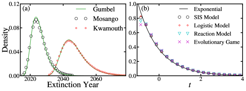
Figure 3: Generalizations to high-dimensional models and Markov chains with internal sinks. (a) Extinction-time distributions for sleeping sickness predicted using a 17-dimensional compartmental model that was fit to case data from the Mosango (large black circles) and Kwamouth (small red circles) regions of the Democratic Republic of Congo (data from Ref. [3]). Mean extinction times (measured from 2016) are approximately 9.5 and 31 years for the Mosango and Kwamouth regions respectively, with standard deviations of 4.8 and 7.9 years. Disease eradication times approximately follow a Gumbel distribution (fit using the mean and variance). (b) Simulations of the SIS, logistic, reaction, and well-mixed evolutionary game models have exponential absorption-time distributions (standardized to zero mean and unit variance) if parameters are chosen so that the dynamics have an internal sink state. For each case, we used $N=50$ and simulated $10^{6}$ trials. See [19] for model details and parameters.

If we study the aforementioned evolutionary game in a well-mixed population, the transition rates vanish linearly as $m\rightarrow 0$ and $m\rightarrow N$ [27, 19]. As discussed above, we expect a convolution of Gumbel distributions with relative weighting $s$ given by the ratio of the linear coefficients at these two boundaries. Figure 1(c) shows that this prediction is borne out in simulations.

In addition to Gumbel and Gaussian classes, other absorption-time distributions arise if the transition rates have power-law decay: $b_{m}+d_{m}=f(N)m^{p}[1+\mathcal{O}(m/N)]$. For $p<1/2$, the decay is sufficiently slow that the normal distribution is maintained: the system still fluctuates at an approximately uniform rate across states. On the other hand, if $p>1/2$ we find a generalized coupon collection phenomenon giving rise to a family of skewed distributions. Slowdown near the boundary dominates the absorption process and the distribution is asymptotic to that for the minimal model $b_{m}=rd_{m}=rm^{p}$ [19]. When $r=0$ the cumulants can be computed analytically: $\tilde{\kappa}_{n}=(n-1)!\zeta(np)/\zeta(2p)^{n/2}$ [5, 8]. Figure 1(d) shows the resulting distributions for a few values of $p$. Interestingly for $p\neq 1$, the shape of the distribution depends subtly on $r$. Figure 2 shows the skew of these distributions as a function of $p$, elucidating the transition from normal distributions to the skewed family.

Beyond simple one-dimensional Markov processes, the eradication-time distributions for African sleeping sickness predicted by a 17-dimensional data-driven model [3] closely resemble the Gumbel [Fig. 3(a)]. This result suggests that the Gumbel distribution is also generic in higher dimensions if the dynamics collapse onto a one-dimensional slow manifold near absorption. Crucially, although the distributions have converged to the Gumbel shape, the fluctuations still matter: the probable extinction times span years. The ratio between the standard deviation and the mean is approximately $0.5$ and $0.25$ for the Mosango and Kwamouth regions respectively. Similar results hold for a variety of high-dimensional systems. Their dynamics are accurately approximated by birth-death processes with transition rates that vanish as a power-law $m^{p}$ near the boundary. Examples include evolutionary dynamics on $D$-dimensional lattices ($p=1-1/D$) and complex networks [28, 5, 8] as well as epidemics on networks [29].

In this Letter we have characterized universality classes for absorption times in birth-death Markov chains. While our results are formulated in terms of the transition rates $b_{i}$ and $d_{i}$, we can also connect the shape of the absorption-time distribution to the spectrum of the transition matrix. Discussion and derivation of these results are provided in the Supplemental Material, sections S2.B and S3.C [19]. Future work might focus on characterizing additional universality classes beyond those studied here. For example, simulations [Fig. 3(b)] show that exponential absorption-time distributions arise frequently in systems with an internal sink state, toward which transitions are more likely [30]. The emergence of the exponential distribution makes sense intuitively: the system quickly settles into a quasiequilibrium mode around the sink, whose slow exponential decay dominates the absorption process [31]. To our knowledge, however, there is no rigorous classification of this case. It would also be fascinating to investigate whether there is a universal crossover between different members of our family of absorption-time distributions. For example, how do the distributions change if the transition rates have mixed decay $m^{p}+\epsilon m^{q}$? Understanding the crossover scaling between these cases will enable the classification for an even broader class of extinction-prone Markov chains.