Learning in Markets: Greed Leads to Chaos but
Following the Price is Right

Abstract

We study learning dynamics in distributed production economies such as blockchain mining, peer-to-peer file sharing and crowdsourcing. These economies can be modelled as multi-product Cournot competitions or all-pay auctions (Tullock contests) when individual firms have market power, or as Fisher markets with quasi-linear utilities when every firm has negligible influence on market outcomes. In the former case, we provide a formal proof that Gradient Ascent (GA) can be Li-Yorke chaotic for a step size as small as $\Theta(1/n)$, where $n$ is the number of firms. In stark contrast, for the Fisher market case, we derive a Proportional Response (PR) protocol that converges to market equilibrium. The positive results on the convergence of the PR dynamics are obtained in full generality, in the sense that they hold for Fisher markets with any quasi-linear utility functions. Conversely, the chaos results for the GA dynamics are established even in the simplest possible setting of two firms and one good, and they hold for a wide range of price functions with different demand elasticities. Our findings suggest that by considering multi-agent interactions from a market rather than a game-theoretic perspective, we can formally derive natural learning protocols which are stable and converge to effective outcomes rather than being chaotic.

1 Introduction

Multi-agent learning in production economies is an important yet underexplored domain. Production economies are classically modelled as Cournot competitions [47] or imperfectly discriminating all-pay auctions (Tullock contests) [28]. In these models, participating firms have market power, and they can significantly influence aggregate outcomes (prices or total exerted effort) with their decisions. However, the advancement of the internet has prompted a rapid paradigm shift in economic competition. Blockchain mining [2, 31], peer-to-peer file sharing [36] and crowdsourcing [34], among others, all constitute distributed production economies with large numbers of small competitors (miners, individuals or firms). In contrast to the classic Cournot or Tullock models, firms that participate in these economies typically engage in multiple concurrent competitions. Moreover, due to their relative small sizes, each firm only has negligible influence on prices and hence, become price-takers. As a result, this form of competition more closely resembles the economic model of Fisher markets in which firms take prices as independently given signals, and purchase optimal bundles of goods (or invest on optimal portfolios to produce goods) given their budget (or capital) constraints.

The question of which adaptive or learning protocols behave well in these economies is largely open and still actively researched. In both Cournot competition and Fisher markets, firms repeatedly observe the aggregate production, and adjust their production outputs over time to improve their own profits. However, empirical results regarding Cournot competition suggest that standard adaptive algorithms, e.g., best response, can lead to rather unstable and irregular adjustments, even in very simple instances (e.g., when there are only two firms and one good) [45, 41, 50]. In contrast, when firms ignore their market power and act as price-takers, the outcomes can be more stable. A line of recent works [51, 52, 5, 16, 15, 17, 9, 18] showed that natural adaptive algorithms, including tâtonnement and proportional response, lead to stable adjustments in many families of Fisher markets, where they converge to market equilibria.

Our contribution.

Motivated by the above, our aim is to study the behavior of learning dynamics in production economies from a theoretical perspective. Our research goals are 1) to establish formal mathematical arguments that explain the irregular behavior of greedy learning rules, such as Gradient Ascent and Best Response dynamics, and 2) to seek protocols that behave well under general conditions. In these directions, we make the following two contributions.

Concerning the first goal, we present the first rigorous mathematical proof that the constant step-size Gradient Ascent (GA) algorithm can exhibit Li-Yorke chaos [37] in Cournot competition (equivalently, in all-pay auctions or Tullock contests) even when the firms are homogeneous. This provides a formal explanation for the unpredictable evolution of these systems that is frequently observed in practice. To derive this result, we leverage Sharkovsky’s theorem which provides a tractable way to verify the conditions in Li-Yorke’s characterization of chaos [40]. In the case of GA, our findings are robust in two aspects: first, chaos emerges for a large family of price functions induced by different demand elasticities, and second, chaos emerges even when the step-size is as small as $\Theta\left(1/n\right)$. Our results in this direction contribute to the growing literature that studies various forms of chaos in game dynamics. [43, 42, 32, 19, 20, 21, 22, 4, 23, 35].

Informally, a dynamical system is Li-Yorke chaotic if there are uncountably many pairs of trajectories which get arbitrarily close together (but never intersect) and move apart indefinitely. When two trajectories are very close to each other, they become essentially indistinguishable due to the precision limitation inherent with the environment or computer. In other words, we cannot tell which of the two trajectories will be realized in the future — this is exactly what unpredictable means. A primary reason for the chaos to arise is that each firm uses its own market power to strategically influence the price. When all firms make such strategic manipulations simultaneously, they aggregately drive prices up and down without proper control.

While the previous technique does not lead to a formal proof of Li-Yorke chaos in the case of Best Response (BR) dynamics, we formalize the (in)-stability properties of the latter via eigenvalue analysis of a first-order linear approximation of the non-linear dynamical system. Here, instability refers to abrupt changes in the long term behavior of the dynamics in response to small perturbations of the systems’ parameters (e.g., firms costs).

Since robustness is an essential property in distributed production economies both from a normative and a descriptive perspective, the above results provide a convincing argument against the use of game-theoretically motivated protocols. This brings us to our second goal which is to seek learning protocols that result in stable outcomes.

Our main result in this direction is to propose a market-motivated Proportional Response (PR) algorithm and show that it is stable and robust: from any initial condition, the PR update rule converges to the market equilibrium of an ensuing Fisher market that captures production economies, namely Fisher market with quasi-linear utility functions. The protocol is simple and can be run by each firm independently using only local and observable (market level) information, which makes it particularly suitable for these distributed settings. It can be interpreted as a naturally motivated adaptive algorithm from a firm’s perspective: in each round, each firm appropriates a certain amount of money, and invests it to the productions of different goods in proportion to the revenues received from selling them in the previous round.

One necessary assumption to establish this result is that as economies grow larger, firms have a negligible influence on aggregate outputs (prices or total exerted efforts). However, we formally argue that in the distributed production economy setting, market equilibria are approximate Nash equilibria. This finding is in line with the largeness concept in [25], who showed that when markets grow large, they become asymptotically efficient even under agents’ strategic behaviors. This implies that the assumption of diminished influence on outcomes does not significantly affect the equilibrium outcome of the system. However, it does have important implications from a technical perspective. In particular, by modeling production economies as Fisher markets, we can leverage their Eisenberg-Gale convex-program formulation [30, 29] to draw direct analogue between our PR algorithm and standard optimization methods like mirror descent. This allows us to apply tools from optimization theory and provides a principled approach to derive proofs of convergence.

Other Related Work.

The Cournot model dates back to the early 19th century [26]. Since then, it became a foundation for many models of production economies [47]. As game theory subsequently matured, the competition between firms was revisited via the popular perspective of Nash equilibrium [39]. The mathematical equivalence between Cournot competition and imperfectly discriminating all-pay auctions with proportional success functions or simply Tullock contests [46] when price functions are isoelastic is documented in [44, 50] (among others). The study of markets is also among the most classical topics in Economics, dating back to [49]. Many markets have efficient equilibria, which is not true in games. But their assumption of non-strategic (i.e., price-taking) behavior of agents is consistently being challenged. Some recent works remedy this by injecting strategic considerations into the market models [1, 13, 12, 3, 8]. [25] showed that when markets grow large, they become asymptotically efficient even under agents’ strategic behaviors; this largeness concept captures the distributed production economies that we study.

[36] were the first to model peer-to-peer networks as distributed markets. Along with [51] who showed convergence of the PR algorithm to equilibria in these models, they stimulated a sequence of works, already discussed above, on the stability of PR algorithms in various applications. Recently, the study of distributed production economies regained traction in the context of the emerging cryptocurrency markets [14]. However, although critical for their stability, the incentives of miners to allocate resources among multiple markets are still not well understood, [6, 31, 33].

Another line of research focuses on explaining the growth of (production) economies in the long run, rather than equilibration in the short run. Recently, [10] proposed a dynamical variant of von Neumann’s pioneering model on economic growth [48]. They showed that the use of PR algorithm to exchange produced goods (which are then used as resources for future productions) leads to universal growth of economies under mild conditions on the efficiencies of the firms.

Finally, various forms of chaos in market dynamics are receiving increasingly more attention  [42, 32, 40, 19, 20, 21, 22, 4, 23, 35].

Paper Outline.

Section 2 presents our three models: Cournot competition with multiple-goods, Tullock contests and Fisher Markets. We discuss their mathematical connections. Section 3 presents our main results: convergence of PR dynamics and chaos and instabilities of GA and BR dynamics. Detailed proofs are delegated to the appendix, but in Sections 4 and 5 we discuss the techniques we use.

2 Models and Definitions

In this section, we describe the Cournot competition and Fisher market models. In their classical descriptions, quantities of goods produced are used as the driving variables to define the notions of Nash and market equilibria. However, it will be more convenient to use spendings/investments on the production of a good as the driving variables here, since this is the domain of the PR algorithm. In all models, $N=\{1,2,\cdots,n\}$ is the set of firms (agents) and $M=\{1,2,\cdots,m\}$ is the set of goods.

Multi-good Cournot Competition (CC) with Isoelastic Demands.

Each firm $i$ invests an amount $b_{ij}\geq 0$ on producing good $j$. We write $\mathbf{b}_{i}:=(b_{ij})_{j\in M}$ and $\mathbf{b}:=\left(\mathbf{b}_{i}\right)_{i\in N}$. Each firm $i$ has only finite amount of capital, $K_{i}$, to invest, thus it is subject to a capital constraint $\sum_{j}b_{ij}\leq K_{i}$. We assume that the marginal cost of producing good $j$ is the same for all firms, which we denote by $\alpha_{j}$. Thus, the quantity of good $j$ produced by firm $i$ is $b_{ij}/\alpha_{j}$. Each good $j$ has isoelastic demand, i.e., the total sales revenue of the good is constant, denoted by $v_{j}$. Thus, the price function for good $j$ is $P_{j}(\mathbf{b})~{}:=~{}v_{j}/\left(\sum_{i}b_{ij}/\alpha_{j}\right)$, and the revenue of firm $i$ received from the sales of good $j$ is $P_{j}(\mathbf{b})\cdot(b_{ij}/\alpha_{j}):=v_{j}\cdot y_{ij}$, where $y_{ij}$ denotes the market share of firm $i$ on good $j$:

$$y_{ij}:=b_{ij}/\sum_{k}b_{kj}.$$ (1)

The profit of firm $i$ is its revenue from the sales of all goods minus its total investment: $\sum_{j}v_{j}y_{ij}-\sum_{j}b_{ij}$.

Tullock Contest (TC).

The above setting admits a correspondence to multiple Tullock contests. According to this interpretation, each firm $i$ invests an amount of $b_{ij}\geq 0$ on producing good $j$, but now the goods are considered as prizes, and the probability that firm $i$ wins good $j$ is $y_{ij}$ as defined in (1). This probabilistic interpretation is natural in the applications of e.g., blockchain mining and imperfectly discriminating all-pay auctions (crowdsourcing). Now, different firms can have different valuations on the prize, so the parameter $v_{j}$ in CC may be distinct for different firms; we let $v_{ij}$ denote the valuation of firm $i$ on good $j$. The expected profit of firm $i$ is

$$u_{i}(\mathbf{b}_{i}):=\sum_{j}v_{ij}y_{ij}-\sum_{j}b_{ij}.$$ (2)

While CC and TC have differences in their rationales, they admit a correspondence in mathematical terms, by replacing deterministic profit in CC with expected profit in TC, and $v_{j}$ with $v_{ij}$ for different firms $i$. Accordingly, we will henceforth refer to this model as CC/TC or simply TC.

Definition 1 (Nash equillibrium).

For any $\delta\geq 0$, we say that $\mathbf{b}^{*}$ is a $\delta$-Nash Equilibrium ($\delta$-NE) of a CC/TC if for each agent $i\in N$,

$$\max_{\mathbf{b}_{i}:\sum_{j}b_{ij}\leq K_{i}}u_{i}(\mathbf{b}_{i},\mathbf{b}^{*}_{-i})\leq(1+\delta)\cdot u_{i}(\mathbf{b}^{*}_{i},\mathbf{b}^{*}_{-i}).$$

In other words, agent $i$ cannot improve her utility by more than an $\delta$ fraction at $\mathbf{b}^{*}$ by unilaterally changing her own investment portfolio. We call a $0$-NE simply a NE.

Fisher Market (FM).

In a Fisher market, each good $j$ has a supply which is normalized to one unit. Again, $b_{ij}$ denotes the spending of firm $i$ on good $j$, and each firm $i$ has a budget of $K_{i}$, so the constraint $\sum_{j}b_{ij}\leq K_{i}$ applies. Let $\mathbf{p}=\left(p_{j}\right)_{j\in M}$, where $p_{j}$ denotes the price of good $j$. At $\mathbf{b}_{i}$, firm $i$ gets $b_{ij}/p_{j}$ units of good $j$ and has a quasi-linear utility function, $u_{i}\left(\mathbf{b}_{i}\mid\mathbf{p}\right)$, which takes the form

$$u_{i}(\mathbf{b}_{i}\mid\mathbf{p})=\sum_{j}v_{ij}\cdot(b_{ij}/p_{j})-\sum_{j}b_{ij},$$ (3)

where $v_{ij}$ denotes firm $i$’s valuation of one unit of good $j$. At price vector $\mathbf{p}$, each firm $i$ select an optimal budget allocation $\mathbf{b}_{i}^{\#}$ in $\operatorname*{arg\,max}_{\mathbf{b}_{i}}u_{i}(\mathbf{b}_{i}\mid\mathbf{p})$ which maximizes its utility subject to the constraint $\sum_{j}b_{ij}\leq K_{i}$. At an optimal budget vector $\mathbf{b}^{\#}_{i}$, a vector $\mathbf{x}^{\#}_{i}:=(b_{ij}^{\#}/p_{j})_{j\in M}$ is called a production bundle of agent $i$ at price vector $\mathbf{p}$.

Definition 2 (Market equilibrium).

A price vector $\mathbf{p}^{\#}=(p^{\#}_{j})_{j\in M}$ is a market equilibrium (ME) if there exists an optimal budget allocation $\mathbf{b}^{\#}=(\mathbf{b}_{i}^{\#})_{i\in N}$ at $\mathbf{p}^{\#}$, such that for each good $j$, $\sum_{i}b^{\#}_{ij}=p^{\#}_{j}$. The vector $\mathbf{b}^{\#}$ is called a market equilibrium spending.

Connection between TC and FM.

The crucial difference between TC and FM is that in TC, prices are determined endogenously as a function of $\mathbf{b}$, whereas in FM, prices are viewed as independent inputs that do not explicitly depend on $\mathbf{b}$. Thus, while both models require each firm $i$ to make an allocation $\mathbf{b}_{i}$ that is subject to the same budget constraint $\sum_{j}b_{ij}\leq K_{i}$, the methods to determine outcomes differ.

However, if $\left(\mathbf{p},\mathbf{b}\right)$ are market equilibrium and market equilibrium spending respectively of an FM, then $\sum_{i}b_{ij}/p_{j}=1$ for each good $j$. Thus, we can translate $b_{ij}/p_{j}$, which is the quantity of good $j$ that firm $i$ gets at the market equilibrium, to the probability that firm $i$ wins good $j$ in the corresponding TC. Under this translation, the outcome in the FM is the same as the outcome in the TC. Due to the well-known properties of Fisher markets, this outcome is Pareto-optimal, and it is envy-free if $K_{i}$ is identical for all $i$.

The above suggest that if there is an algorithm that converges to the market equilibrium spending (our Theorem 4 establishes this) of the FM, then it yields a feasible solution of the corresponding TC. The remaining question is the quality of this feasible solution, i.e., how close it is to a Nash equilibrium of the TC. It turns out that if the underlying distributed production economy satisfies a natural largeness property, then the market equilibrium spending is also a $\delta^{\prime}$-NE for some small $\delta^{\prime}>0$. In particular, as we show in Proposition 3 below, this is the case if the budget of each firm is small compared to any market equilibrium price, i.e., if $\max_{i,j}\{K_{i}/p^{\#}_{j}\}\leq\delta$ for a small $\delta>0$. We may view $\delta$ as a parameter that describes the largeness of the economy: the smaller $\delta$ is, the larger the economy is. (We also need the bang-per-buck ratio $\beta_{i}:=\max_{j}\{v_{ij}/p^{\#}_{j}\}$ to be sufficiently high for all firms $i$, because otherwise a firm might invest nothing thus attain zero utility, forcing $\delta^{\prime}$ to be $+\infty$.)

Proposition 3.

Suppose that $\mathbf{b}^{\#}$ is a market equilibrium spending vector of a quasi-linear FM, and $\mathbf{p}^{\#}$ is the corresponding market equilibrium price vector. For every $i\in N$, let $\beta_{i}:=\max_{j}\{v_{ij}/p^{\#}_{j}\}$. If $\max_{i,j}\{K_{i}/p^{\#}_{j}\}\leq\delta$, then $\mathbf{b}^{\#}$ is also a $\delta^{\prime}$-NE of the corresponding TC, where $\delta^{\prime}=\max_{i:\beta_{i}>1}\left\{\left(\frac{\beta_{i}}{1-\delta}-1\right)/\left(\beta_{i}-1\right)\right\}-1$, provided that there is no firm $k$ with $1-\delta<\beta_{k}<1$.

It is easy to see that if $\min_{i}\{\beta_{i}\}$ grows, then $\delta^{\prime}$ tends toward $\delta/(1-\delta)$. The proof of Proposition 3 can be found in Section A.1.

3 Our Main Results

We present our two main results here. We discuss the methodology of proving them in Sections 4 and 5.

Proportional Response (PR) in Quasi-linear Fisher Market.

In a quasi-linear Fisher market, our PR protocol starts with each firm $i\in N$ investing an arbitrary portfolio $\mathbf{b}_{i}^{\circ}$ which is positive, i.e., $b_{ij}^{\circ}>0$ for all $j\in M$. In each round, firms update their portfolios simultaneously according to the PR-QLIN protocol in Algorithm 1.

The PR-QLIN protocol can be naturally interpreted. After all firms update their investment portfolios in round $t$, one unit of each good $j$ is allocated to the firms in proportion to their investments on the good. Thus, firm $i$ gets $y_{ij}^{t}$ units of good $j$ (line 3). Then each firm $i$ computes its attained utility, $S_{i}^{t}$, without subtracting investment cost (line 5). If $S_{i}^{t}>K_{i}$, then firm $i$ will appropriate all of its capital, $K_{i}$, for investment in round $t+1$; otherwise it will only appropriate an amount of $S_{i}^{t}$ for investment. Then each firm invests its appropriated capital on each good in proportion to the utility attained from that good in the previous round, i.e., firm $i$ invests a fraction of $v_{ij}y_{ij}^{t}/S_{i}^{t}$ of its appropriated capital on good $j$. Our main result is stated below.

Theorem 4.

Given any positive starting point $\mathbf{b}^{\circ}$, the algorithm PR-QLIN converges to the set of market equilibrium spending vectors of the quasi-linear Fisher market.

Algorithm 1 PR-QLIN Learning Protocol

Input: $\left(K_{i},v_{i1},v_{i2},\ldots,v_{im},\mathbf{b}_{i}^{\circ}\right)$ for each firm $i$
Output: market equilibrium spending $\mathbf{b}^{\#}$.

1:for $t=0,1,2,\ldots$ do

2:     for every firm $i$ and good $j$ do

3:         $y_{ij}^{t}\leftarrow b_{ij}^{t}/\sum_{k}b_{kj}^{t}$      

4:     for every firm $i$ do

5:         $S_{i}^{t}\leftarrow\sum_{j}v_{ij}y_{ij}^{t}$

6:         for every good $j$ do

7:              if $S_{i}^{t}>K_{i}$ then

8:                  $b_{ij}^{t+1}\leftarrow(v_{ij}y_{ij}^{t}/S_{i}^{t})\cdot K_{i}$

9:              else

10:                  $b_{ij}^{t+1}\leftarrow v_{ij}y_{ij}^{t}$ $\lx@algorithmicx@hfill\left(\triangleright\right)\text{same as }(v_{ij}y_{ij}^{t}/S_{i}^{t})\cdot S_{i}^{t}$                             

Gradient Ascent Dynamics and Li-Yorke Chaos.

To establish our chaos results of the GA dynamics in CC (hence, also in TC), we consider a CC with one good and $n$ firms. Since there is only one good, we omit the subscript $j=1$ and use the shorthand $\alpha\equiv\alpha_{1}$ to denote the marginal cost of producing the good (recall from Section 2 that this is equal for all firms). In this setting, it is more convenient to use the quantities of the good produced, i.e., the variables $x_{i}=b_{i1}/\alpha$, as the driving variables. Without loss of generality, let $v_{1}=1$. Then the utility of firm $i$ is $u_{i}(\mathbf{x})=x_{i}/(\sum_{k}x_{k})-\alpha x_{i}$. The Gradient Ascent (GA) update rule is given by $x_{i}^{t+1}\leftarrow x_{i}^{t}+\eta\cdot\nabla_{i}u_{i}\left(\mathbf{x}^{t}\right)$, where $\eta$ is the step-size.

Assuming that the initial point is symmetric, i.e., that $x_{i}^{\circ}$ is identical for all $i$, then, in each round $t>0$, the $x_{i}^{t}$’s remain identical for all $i$. Thus, a symmetric GA dynamic is essentially one-dimensional, and its trajectory can be represented by the sequence $\{x_{1}^{t}\}_{t\geq 0}$ generated by the GA update rule:

$$\textstyle x_{1}^{t+1}\leftarrow x_{1}^{t}+\eta\cdot\left(\frac{n-1}{n^{2}x_{1}^{t}}-\alpha\right).$$ (4)

Our main result states that even for such an apparently simple one-dimensional dynamical system, chaos occurs with step-size $\eta$ as small as $\Theta(1/n)$. Here, we refer to Li-Yorke chaos which is formally defined below.

Definition 5 (Li-Yorke Chaos).

A discrete time dynamical system $\left(x^{t}\right)_{t\in\mathbb{N}}$ such that $x^{t}:=f^{t}\left(x^{\circ}\right)$ for a continuous update rule $f:X\to X$ on a compact set $X\subseteq\mathbb{R}$ is called Li-Yorke chaotic, if (i) for each $k\in\mathbb{N}$, there exists a periodic point $\hat{x}\in X$ with period $k$, and (ii) there is an uncountably infinite set $S\subset X$ that is scrambled, i.e., if for each $x\neq x^{\prime}\in S$ it holds that $\lim\inf_{t\to\infty}|f^{t}\left(x\right)-f^{t}\left(x^{\prime}\right)|=0<\lim\sup_{t\to\infty}|f^{t}\left(x\right)-f^{t}\left(x^{\prime}\right)|$.

Theorem 6 (Li-Yorke Chaos in $n$-Player CC/TC).

Consider a symmetric GA dynamic with $n$ firms and marginal cost $\alpha>0$. Then for any step-size $\eta\geq 3(n-1)/n^{2}\alpha^{2}$, the essentially-one-dimensional dynamical system (4) is Li-Yorke chaotic.

This theorem applies with isoelastic price function. In Section 5, we consider a larger family of price functions and prove that Li-Yorke chaos also occurs in the corresponding symmetric GA dynamics. We also present theoretical and empirical evidences that instability arises when the GA rule is replaced by the Best Response rule.

Remark.

In practice, firms may choose to use a large step-size in a myopic, greedy approach to profit maximization. Given that chaos occurs with a vanishingly small step-size $\Theta\left(1/n\right)$ as the number of firms increases (cf. Theorem 6), our result is practically relevant for distributed production economies in which many small firms are involved. Stability results should be possible for smaller step sizes, however, such step sizes are not particularly interesting from a practical perspective. Finally, the presence of a centralised planner who may enforce small step sizes is a rather unnatural assumption for the settings and applications that we consider.

4 Proportional Response Dynamics

Program	Description	Variables
(EG)	Eisenberg-Gale	$x_{ij}$	$=$	allocations	$i\in N,j\in M$
(D)	Dual	$p_{j}$	$=$	prices	$j\in M$
(TD)	Transformed dual	$q_{j}$	$=$	$\ln{\left(p_{j}\right)}$	$j\in M$
(SH)	Shmyrev-type	$b_{ij}$	$=$	spending	$i\in N,j\in M$

Figure 1: Convex programs in the derivation of the PR-QLIN protocol via the Mirror Descent (MD) protocol. Starting from the dual (D) of a generalized Eisenberg-Gale convex program (EG), we go to the transformed dual (TD) and by convex duality to a Shmyrev-type primal program (SH) which is hence, equivalent to the initial program (EG). The objective functions of (SH) for quasi-linear utilities is 1-Bregman convex which implies convergence of the MD protocol.

Our proof of Theorem 4 consists of two major steps. In the first, we derive a convex program that captures the market equilibrium (ME) spending of the quasi-linear Fisher market via the approach of [5, 24, 17]. In the second, we show that a general Mirror Descent (MD) algorithm converges to the optimal solution of this convex program; PR-QLIN is an instantiation of this MD algorithm.

Convex Program Framework.

We first utilize a convex optimization framework to derive a convex program that captures the ME spendings of any quasi-linear FM. The ensuing framework is summarized in Figure 1. In short, via duality and variable transformations, the market equilibria of a FM can be captured by various convex programs, each with a different domain. Our starting point is a convex program proposed by [27] that captures ME prices of quasi-linear Fisher market (which belongs to type (D) in Figure 1). From this, we derive a new convex program with captures the ME spendings of the market (which belongs to type (SH)); see Section A.2 for the details. The convex program is

$$\min_{\mathbf{b},\mathbf{w},\mathbf{p}} ~{}~{}-\sum_{i=1}^{n}\sum_{j=1}^{m}b_{ij}\ln{v_{ij}}+\sum_{i=1}^{n}w_{i}+\sum_{j=1}^{m}p_{j}\ln{p_{j}}$$

s.t. $$\sum_{i=1}^{n}b_{ij}=p_{j},\hskip 38.0pt\forall j\in M,$$

$$\sum_{j=1}^{m}b_{ij}+w_{i}=K_{i},~{}~{}~{}\forall i\in N,$$ (SH)

$$b_{ij},w_{i}\geq 0,\hskip 47.0pt\forall i\in N,j\in M.$$

For convenience, we will write $F(\mathbf{b},\mathbf{w},\mathbf{p}):=-\sum_{i=1}^{n}\sum_{j=1}^{m}b_{ij}\ln{v_{ij}}+\sum_{i=1}^{n}w_{i}+\sum_{j=1}^{m}p_{j}\ln{p_{j}}$. Observe that the first and second constraints determine the values of $\mathbf{w},\mathbf{p}$ in terms of $b_{ij}$’s. Thus, we can rewrite the convex program to have variables $\mathbf{b}$ only, and the remaining constraints are $b_{ij}\geq 0$ and $\sum_{j=1}^{m}b_{ij}\leq K_{i}$; we slightly abuse notation by using $F(\mathbf{b})$ to denote the objective of this convex program.

From Mirror Descent to Proportional Response.

After having the convex program with variables $\mathbf{b}$ only, we can compute a ME spending by the optimization algorithm of Mirror Descent (MD). To begin, we recap a general result about MD [11, 5].

Definition 7 (KL-divergence and $L$-Bregman convexity).

Let $C$ be a compact and convex set and let $h$ be a convex function on $C$. Then, for any $\mathbf{z}^{\prime}\in C,\mathbf{z}\in\mathsf{rint}(C)$ where $\mathsf{rint}(C)$ is the relative interior of $C$, the Bregman divergence, $d_{h}\left(\mathbf{z}^{\prime},\mathbf{z}\right)$, generated by $h$ is defined by

$$d_{h}(\mathbf{z}^{\prime},\mathbf{z}):=h(\mathbf{z}^{\prime})-\left[h(\mathbf{z})+\left\langle\nabla h(\mathbf{z}),\mathbf{z}^{\prime}-\mathbf{z}\right\rangle\right].$$

The Kullback-Leibler (KL) divergence between $\mathbf{z}^{\prime}$ and $\mathbf{z}$ is defined by $\mathrm{KL}(\mathbf{z}^{\prime}\|\mathbf{z}):=\sum_{j}z^{\prime}_{j}\cdot\ln\frac{z^{\prime}_{j}}{z_{j}}-\sum_{j}z^{\prime}_{j}+\sum_{j}z_{j}$, which is the same as the Bregman divergence $d_{h}$ with regularizer $h\left(\mathbf{z}\right):=\sum_{j}(z_{j}\cdot\ln z_{j}-z_{j})$. A function $F$ is $L$-Bregman convex w.r.t. the Bregman divergence $d_{h}$ if for any $\mathbf{z}^{\prime}\in C$ and $\mathbf{z}\in\mathsf{rint}(C)$, $F(\mathbf{z})+\left\langle\nabla F(\mathbf{z}),\mathbf{z}^{\prime}-\mathbf{z}\right\rangle\leq f(\mathbf{z}^{\prime})\leq f(\mathbf{z})+\left\langle\nabla f(\mathbf{z}),\mathbf{z}^{\prime}-\mathbf{z}\right\rangle+L\cdot d_{h}(\mathbf{z}^{\prime},\mathbf{z})$.

For the problem of minimizing a convex function $F(\mathbf{z})$ subject to $\mathbf{z}\in C$, the MD protocol w.r.t. the KL divergence is presented in Algorithm 2. In the protocol, $1/\Gamma$ is the step-size, which may vary with $t$ (and typically diminishes with $t$). However, in the current application of distributed dynamics, a time-varying step-size is undesirable or even impracticable, since it requires firms to keep track of a global clock.

Algorithm 2 MD protocol w.r.t. $\mathrm{KL}$-divergence

Input: A convex set $C$, a function $F$ defined on $C$, a parameter $\Gamma$ and a point $\mathbf{z}^{\circ}\in C$.
Output: $\mathbf{z}^{*}=\operatorname*{arg\,min}_{\mathbf{z}\in C}F(z)$.

1:for $t=0,1,2,\ldots$ do

2:     $g\left(\mathbf{z},\mathbf{z}^{t}\right)\leftarrow\left\langle\nabla F(\mathbf{z}^{t}),\mathbf{z}-\mathbf{z}^{t}\right\rangle+\Gamma\cdot\mathrm{KL}(\mathbf{z}\|\mathbf{z}^{t})$

3:     $\mathbf{z}^{t+1}\leftarrow\operatorname*{arg\,min}_{\mathbf{z}\in C}\{g\left(\mathbf{z},\mathbf{z}^{t}\right)\}$

Theorem 8.

Suppose $F$ is an $L$-Bregman convex function w.r.t. the Bregman divergence $d_{h}$, and $\mathbf{z}^{t}$ is the point reached after $t$ applications of the MD update rule in Algorithm 2 with parameter $\Gamma=L$. Then $F(\mathbf{z}^{t})-F(\mathbf{z}^{*})~{}\leq~{}L\cdot d(\mathbf{z}^{*},\mathbf{z}^{\circ})/t,$ where $\mathbf{z}^{*}=\operatorname*{arg\,min}_{\mathbf{z}\in C}F(z)$.

In Appendix B, we first prove Lemma 9 below. Then, we show that PR-QLIN is an instantiation of Algorithm 2 with $\Gamma=1$. This is achieved by identifying the variables $\mathbf{b}$ in PR-QLIN as the variables $\mathbf{z}$ in Algorithm 2, and the domain $\{\mathbf{b}~{}|~{}b_{ij}\geq 0~{}\text{and}~{}\sum_{j=1}^{m}b_{ij}\leq K_{i}\}$ as the convex set $C$ in Algorithm 2. Thus, Theorem 8 guarantees the updates of PR-QLIN converge to an optimal solution of the convex program (SH), and hence Theorem 4 follows.

Lemma 9.

The objective function $F(\mathbf{b})$ of (SH) is a $1$-Bregman convex function w.r.t. the KL-divergence.

5 Gradient Ascent & Best Response Dynamics

To establish the statement of Theorem 6 about the GA dynamics in equation (4) for $n=2$ (the technique is similar for any $n>2$), let $f\left(x\right):=x+\eta\left(\frac{1}{4x}-\alpha\right)$. To prove that Li-Yorke chaos occurs, we use a seminal theorem of [37], which states that if $f$ has two easy-to-verify properties, then the dynamical system is Li-Yorke chaotic. The two properties are: (i) an invariant set of $f$ that includes a fixed point $x^{*}$, i.e., an interval $I=[L,U]$ such that $f\left(I\right)\subseteq I$ with a point $L<x^{*}<U$ satisfying $f(x^{*})=x^{*}$, and (ii) a point $x^{\prime}\in I$ other than $x^{*}$ with period $3$, i.e., $f^{\left(3\right)}\left(x^{\prime}\right)=x^{\prime}$, where $f^{\left(3\right)}\left(x\right):=\left(f\circ f\circ f\right)\left(x\right)$. These properties are formally established in Lemma 13 and Proposition 14 respectively. A visualization of Theorem 6 is provided in the first two panels of Figure 2. It can be seen that chaos may emerge even for small step-size and for asymmetric marginal costs.

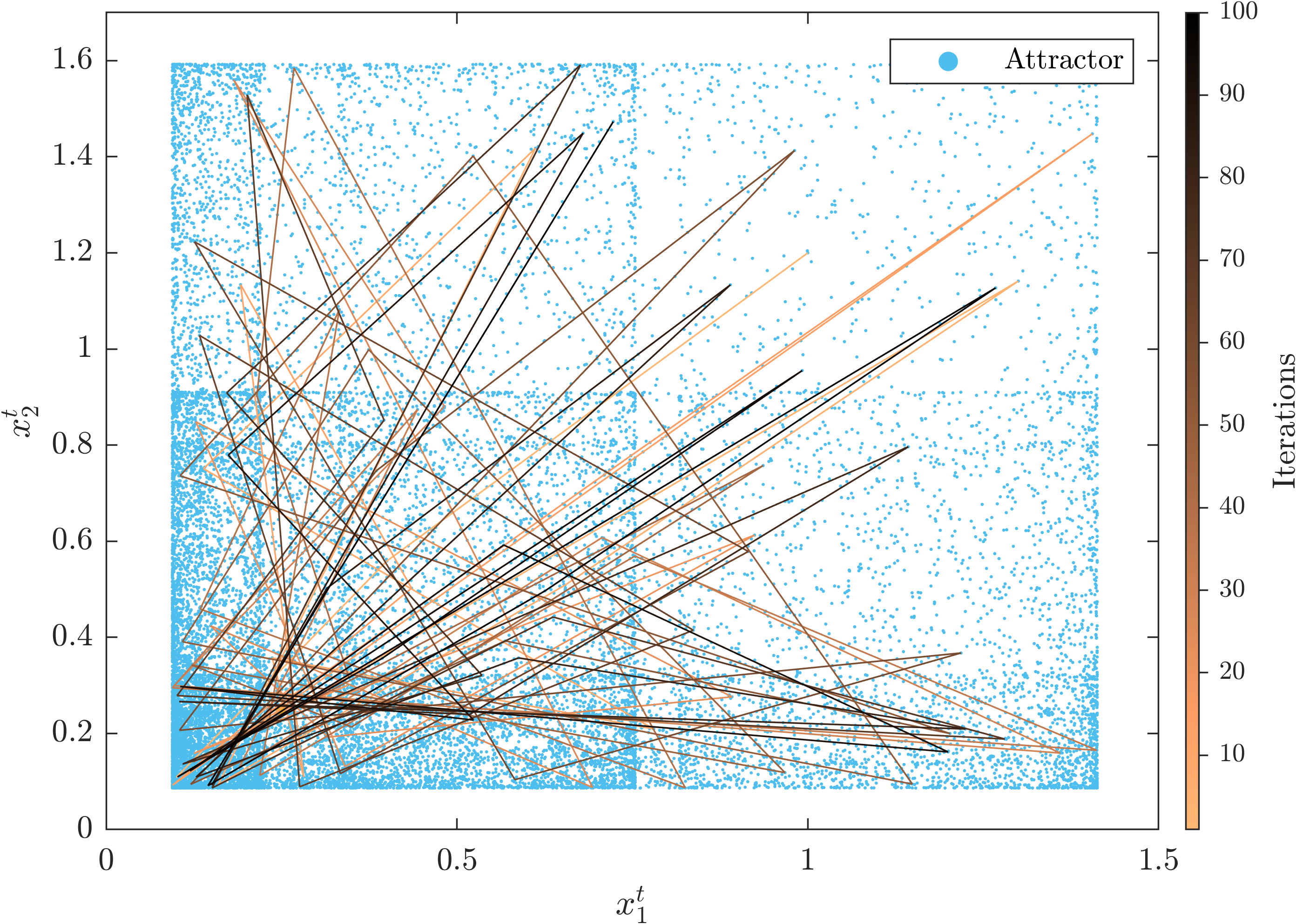
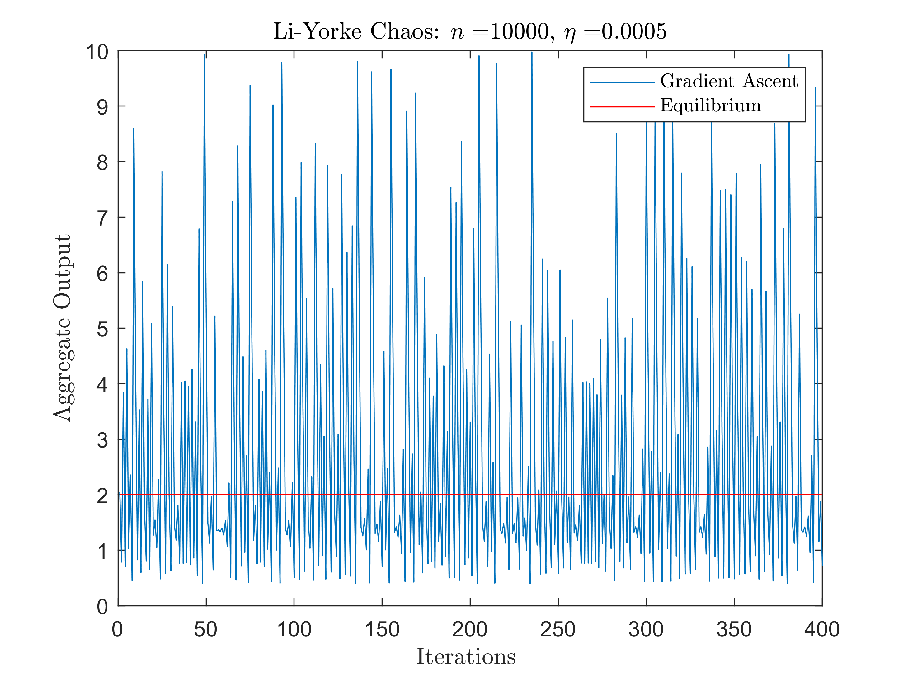
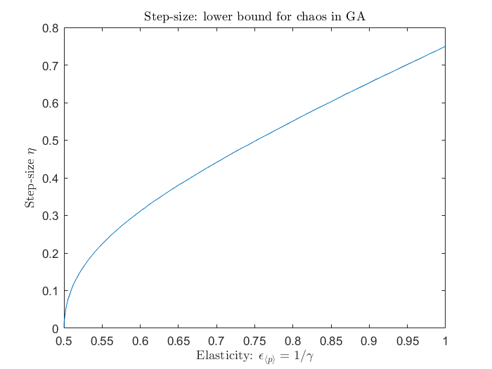
Figure 2: Li-Yorke chaos of the Gradient Ascent (GA) dynamics with constant step-size in $n$-firm Cournot competition with isoelastic inverse demand function (equivalently, Tullock contest with proportional success function). First panel: chaotic trajectories (light to dark lines) of the output pairs of two firms that start from different initial outputs for $t\in[1,200]$. The planar dots denote their projections for $t\in[1,10^{4}]$ and fill the plane as $t$ grows. Second panel: aggregate output in a market with $n=10^{4}$ firms with different costs $a_{i}\in[10^{-5},1],i=1,\dots,10^{4}$ starting from a randomly selected initial output vector and using GA with step-size $\eta=5\cdot 10^{-4}$ for $t\in[0,400]$. Third panel: Minimum step-size for which chaos provably occurs under the GA update rule in 2-firm Cournot competition with inverse demand function $\left(x_{1}+x_{2}\right)^{-\gamma}$, for $\gamma>0$. Interestingly, chaotic behavior is more likely when demand is inelastic.

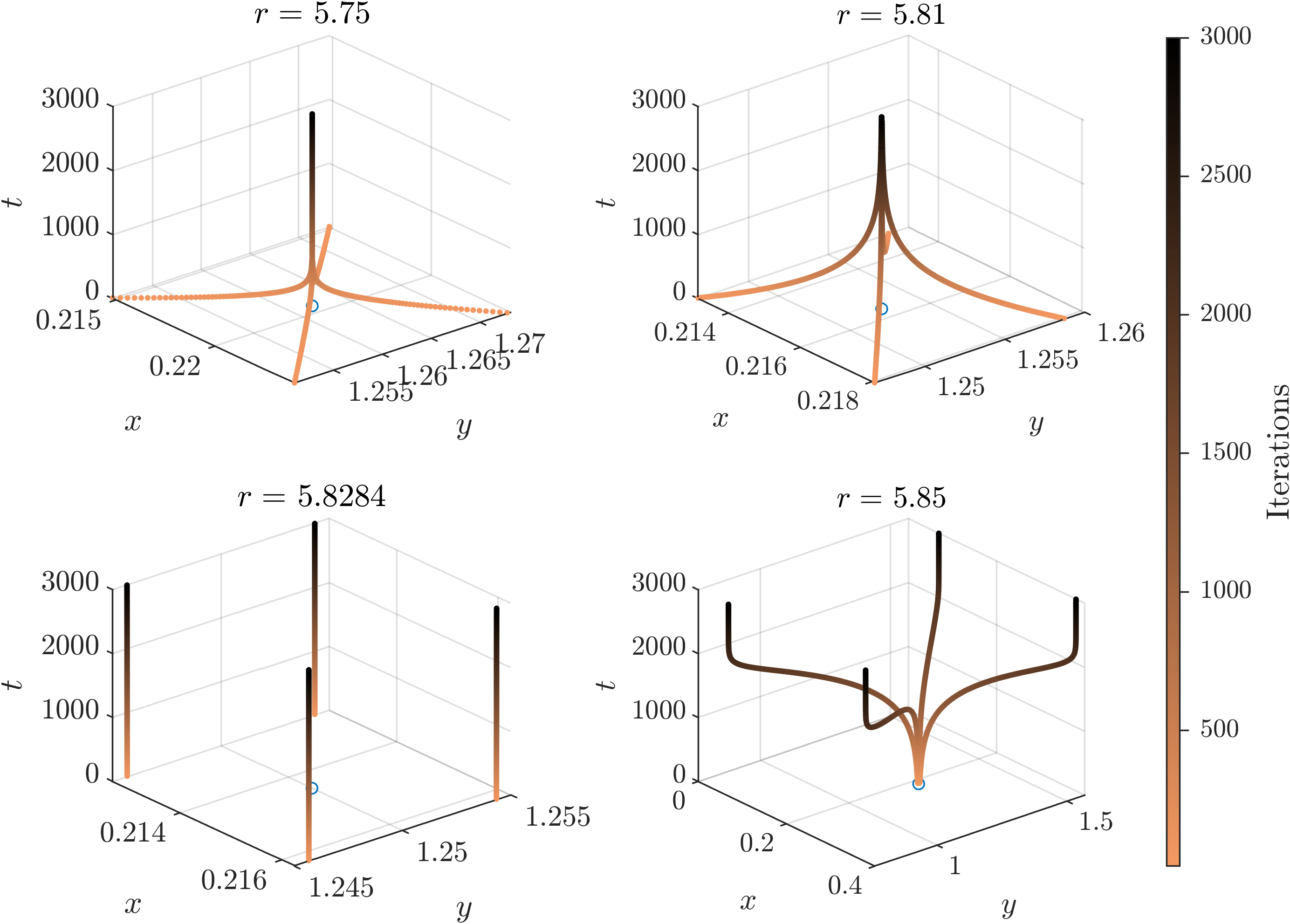
Figure 3: Firms’ outputs $\left(x^{t},y^{t}\right)$ (horizontal plane) with respect to time $t\in[10,250]$ (vertical axis). Parameter $r$ captures the cost asymmetry between the two firms. The dynamics spiral inwards towards the equilibrium (red circle on the $\left(x,y\right)$-plane) for lower asymmetry between the two firms (upper panels), cycle around the equilibrium when $r$ is equal to the critical level $r_{0}\approx 5.8284$ (bottom left panel) and spiral outwards (till they become cyclic) for values of $r>r_{0}$ (bottom right panel). This is in agreement with Proposition 15 in Appendix C which shows that the attractors of the BR dynamics may change significantly for only small perturbations in the system parameters as expressed by the cost asymmetry-ratio $r$.

General Price Functions.

The emergence of chaos is not tied to the particular choice of the isoelastic price function of the form $v_{1}/X$, where $X:=\sum_{i}x_{i}$. More generally, we may consider the parametric price function $X^{-\gamma}$, where $\gamma>0$ is the inverse of the demand elasticity $\varepsilon_{\langle p\rangle}$. This is a special case of the more general price functions $P\left(X\right)=A+BX^{-\gamma}$, see e.g., [38], for $A=0,B=1$ and $\gamma>0$. For these functions, we verify the two conditions required in the theorem of Li and Yorke, for a range of choices of $\gamma$ numerically (via computer software). The lower bound of the step-size $\eta$ at which chaos emerges (in the symmetric case) is depicted in the third panel of Figure 2. The interesting observation is that chaos is more likely for less elastic demand.

Best Response Dynamics.

We conclude by revisiting the well-studied Best Response (BR) dynamics and formally establish that they can be unstable even in the simplest setting of two firms and one good. The general BR update rule is $x_{i}^{t+1}\leftarrow\operatorname*{arg\,max}_{x_{i}}u_{i}(x_{i},x_{-i}^{t})$. For TC with isoelastic demand, the BR dynamics take the form $x_{i}^{t+1}\leftarrow\sqrt{x_{-i}^{t}/\alpha_{i}}-x_{-i}^{t},$ for $i=1,2$, where $\alpha_{i}$ is the marginal cost of firm $i$. BR dynamics in Cournot duopoly with isoelastic functions have been (empirically) studied by [41] and, in the framework of contests, in [50]. Both papers suggest that the stability of the unique fixed point, $\left(x_{1}^{*},x_{2}^{*}\right)$, depends on the degree of asymmetry between the two firms, captured by the ratio $r:=\alpha_{1}/\alpha_{2}$ with instabilities emerging as the asymmetry increases. While our previous technique does not lead to a formal proof of Li-Yorke chaos in BR dynamics, we formalize the (in)-stability properties of the latter via eigenvalue analysis of a first-order linear approximation of the original non-linear system, cf. Proposition 15. The result is visualized in Figure 3 which shows how the trajectories of the dynamics may change dramatically in response to even small perturbations of the model parameters (firms’ costs).

6 Conclusions

The current work brings together multi-agent learning with optimization, market theory and chaos theory. Our findings suggest that by considering production economies from a market rather than a game-theoretic perspective, we can formally derive a natural learning protocol (PR) which is stable and converges to effective outcomes rather than being chaotic (GA). Due to its simple form and mild informational requirements, PR can be used to study real-world multi-agent settings from an AI perspective. Since distributed production economies capture many important applications (blockchain, peer-to-peer networks, crowdsourcing), our contributions are significant both for theoretical and practical purposes.

Appendix A Convex Programs and Equilibrium Characterizations

In this appendix, we prove Proposition 3. To do so, our first task is to characterise the Nash equilibria of the multi-good Cournot competition (CC) and simultaneous Tullock contests (TC) models and compare them to the Market equilibria of the ensuing Fisher Market with quasi-linear utilities. This can be conveniently done by expressing all relevant quantities via proper convex optimization problems and leveraging techniques from convex duality. These are done in Sections A.1 and A.2. The proof of Proposition 3 is presented in Section A.3.

A.1 Nash Equilibria in Cournot Competition and Tullock Contests

To proceed, let $\Gamma=\left(N,M,\left(u_{i}\right)_{i\in N}\right)$ denote a CC or TC model and recall that a Nash equilibrium $\mathbf{b}^{*}=\left(\mathbf{b}^{*}_{i}\right)_{i\in N}$ of is a strategy profile such that the strategy $\mathbf{b}_{i}^{*}=\left(b^{*}_{i,j}\right)_{j\in M}$ of each firm $i\in N$ maximizes its own utility given the strategies $\mathbf{b}^{*}_{-i}$ of the other players. Setting $p_{j}:=\sum_{i=1}^{n}b_{ij}$, for each $j\in M$, the equilibrium strategy $\mathbf{b}_{i}^{*}$ can be expressed as the solution of the following maximization problem

$$\max_{\mathbf{b}_{i}}\,\, u_{i}\left(\mathbf{b}_{i};\mathbf{b}^{*}_{-i}\right)=\sum_{j=1}^{m}b_{ij}\left(\frac{v_{ij}}{p_{j}}-1\right)$$

s.t. $$\sum_{j=1}^{m}b_{ij}\leq K_{i},$$ (NE)

$$b_{ij}\geq 0,\qquad\quad\forall j\in M.$$

The following characterization stems from the first-order conditions.

Proposition 10.

At any Nash Equilibrium, $\mathbf{b}^{*}=\left(\mathbf{b}^{*}_{i}\right)_{i\in N}$, of $\Gamma$, it holds that

1. If firm $i$ exhausts its capacity, i.e., if $\sum_{j=1}^{m}b^{*}_{ij}=K_{i}$, then there exists a constant $C_{i}^{*}\geq 1$ such that

   $$\left(v_{ij}/p^{*}_{j}\right)\left(1-b^{*}_{ij}/p^{*}_{j}\right)\leq C_{i}^{*},\quad\forall j\in M,$$

   with equality whenever $b^{*}_{ij}>0$ for $j\in M$.

2. If firm $i$ does not exhaust its capacity, i.e., if $\sum_{j=1}^{m}b^{*}_{ij}<K_{i}$, then

   $$\left(v_{ij}/p^{*}_{j}\right)\left(1-b^{*}_{ij}/p^{*}_{j}\right)\leq 1,\quad\forall j\in M,$$

   with equality whenever $b^{*}_{ij}>0$ for $j\in M$.

Proof.

By differentiating $u_{i}\left(\mathbf{b}\right)$ with respect to $b_{ij}$, we obtain

$$\frac{\partial}{\partial b_{ij}}u_{i}\left(\mathbf{b}\right) =\frac{v_{ij}}{p_{j}}-1+b_{ij}\left(-\frac{v_{ij}}{p_{j}^{2}}\right)=\frac{v_{ij}}{p_{j}}\left(1-\frac{b_{ij}}{p_{j}}\right)-1$$

and

$$\frac{\partial^{2}}{\partial b^{2}_{ij}}u_{i}\left(\mathbf{b}\right) =\frac{2v_{ij}}{p_{j}}\left(\frac{b_{ij}}{p_{j}}-1\right)\leq 0,$$

where the last inequality follows from the fact that $b_{ij}\leq p_{j}=\sum_{k\in N}b_{kj}$. This shows that the function $u_{i}\left(\mathbf{b}_{i};\mathbf{b}_{-i}\right)$ is concave in $b_{i}$ for all $\mathbf{b}_{-i}$. Hence, the first order conditions for the Nash equilibrium can be formulated as follows.

Case 1:

$\sum_{j=1}^{m}b^{*}_{ij}=K_{i}$. The capacity constraint is satisfied with equality (tight), i.e., player $i$ exhausts its effort capacity in equilibrium. In this case, there exists a constant $C_{i}^{*}\geq 1$ such that

(a)	if $b_{ij}>0$: $\frac{\partial}{\partial b_{ij}}u_{i}\left(\mathbf{b}\right)=C_{i}^{*}$
(b)	if $b_{ij}=0$: $\frac{\partial}{\partial b_{ij}}u_{i}\left(\mathbf{b}\right)\leq C_{i}^{*}$.

To see this, assume by contradiction that there exist $b^{*}_{ij}$ and $b^{*}_{ij^{\prime}}$ with $\frac{\partial}{\partial b_{ij}}u_{i}\left(\mathbf{b}^{*}\right)>\frac{\partial}{\partial b_{ij^{\prime}}}u_{i}\left(\mathbf{b}^{*}\right)$. Then, by using a first-order approximation, the strategy profile

$$\mathbf{b}^{\prime}_{i}=\begin{cases}b_{ik},&\text{for }k\neq j,j^{\prime}\\ b_{ij}+\delta,&\text{for }k=j\\ b_{ij^{\prime}}-\delta,&\text{for }k=j^{\prime}\\ \end{cases}$$

is still feasible for (NE) and yields a higher payoff to player $i$ than $\mathbf{b}^{*}_{i}$ which contradicts the fact that $\mathbf{b}_{i}^{*}$ is a best response to $\mathbf{b}^{*}_{-i}$. The constraint $C_{i}^{*}\geq 1$ stems from $C_{i}^{*}\geq 0$ and by rescaling it with the constant $-1$ that appears in the partial derivative of $u_{i}$.

Case 2:

$\sum_{j=1}^{m}b^{*}_{ij}<K_{i}$. The capacity constraint is satisfied with inequality (not tight). In this case,

(a)	if $b_{ij}>0$: $\frac{\partial}{\partial b_{ij}}u_{i}\left(\mathbf{b}\right)=0$
(b)	if $b_{ij}=0$: $\frac{\partial}{\partial b_{ij}}u_{i}\left(\mathbf{b}\right)\leq 0$.

Since the capacity constrain is not binding, these are essentially the conditions for unconstrained maximization except for the non-negativity constrains on the $b_{ij}$’s for $i\in N,j\in M$. If not all partial derivatives are equal to zero (less or equal than zero if $b_{ij}=0$), then firm $i$ could increase its utility by increasing (decreasing) its effort $b_{ij}$ in any contest $j$ with positive (negative) partial derivative and still remain in the feasible region of (NE). ∎

A.2 Market Equilibria of Quasi-Linear Fisher Markets

We begin by stating a convex program that captures the market equilibrium prices of a quasi-linear Fisher market [27, 24]:

$$\min_{p,\beta}\quad \sum_{j=1}^{m}p_{j}~{}-~{}\sum_{i=1}^{n}K_{i}\ln{\beta_{i}}$$

s.t. $$v_{ij}\beta_{i}\leq p_{j},~{}~{}~{}\forall i\in N,j\in M,$$ (D)

$$\beta_{i}\leq 1,\hskip 28.0pt\forall i\in N.$$

To study the relationship between market equilibria (solutions of (D)) and Nash equilibria (first-order conditions in Proposition 10), we consider the following equivalent problem by taking the logs of the constraints and letting $q_{j}:=\ln{p_{j}}$ and $\gamma_{i}:=-\ln{\beta_{i}}$ for all $i\in N,j\in M$.

$$\min_{q,\gamma}\quad \sum_{j=1}^{m}\exp(q_{j})~{}+~{}\sum_{i=1}^{n}K_{i}\,\gamma_{i}$$

s.t. $$q_{j}+\gamma_{i}\geq\ln{v_{ij}},~{}~{}~{}\forall i\in N,j\in M,$$ (TD)

$$\qquad\,\gamma_{i}\geq 0,\hskip 28.0pt\forall i\in N.$$

where the constraints $\gamma_{i}\geq 0$ correspond to the initial constraints $\beta_{i}\leq 1$ for all $i\in N$. We can now construct the dual of (TD) and gain intuition about our original problem.

Lemma 11.

The dual of (TD) is given by

$$\max_{b,w,p}\,\, \sum_{i=1}^{n}\sum_{j=1}^{m}b_{ij}\ln{v_{ij}}~{}-~{}\sum_{j=1}^{m}p_{j}\ln{p_{j}}~{}-~{}\sum_{i=1}^{n}w_{i}$$

s.t. $$\sum_{i=1}^{n}b_{ij}=p_{j},\hskip 38.5pt\forall j\in M,$$

$$\sum_{j=1}^{m}b_{ij}+w_{i}=K_{i},~{}~{}~{}\forall i\in N,$$ (SH)

$$b_{ij},w_{i}\geq 0,\hskip 47.0pt\forall i\in N,j\in M.$$

Variable $b_{ij}$ can be physically interpreted as the spending of player $i\in N$ on good $j\in M$. Accordingly, variable $w_{i}$, corresponds to the unspent budget of firm $i\in N$. While variable $w_{i}$ can be eliminated via the second constraint in the convex program, it will be useful to retain it in describing the solution of (SH) (see Proposition 12).

Proof.

Let $\mathcal{L}\left(\left(q,\gamma\right),\left(b,p,w\right)\right)$ denote the Lagrange function of (TD), where $\left(q,\gamma\right)$ denote the primal variables and $\left(b,p,w\right)$ the dual variables (to be properly defined). Then, we have that

$$\mathcal{L}\left(\left(q,\gamma\right),\left(b,p,w\right)\right) =\sum_{j=1}^{m}\exp{q_{j}}+\sum_{i=1}^{n}K_{i}\gamma_{i}+\sum_{i=1}^{n}\sum_{j=1}^{m}b_{ij}\left(\ln{v_{ij}}-\gamma_{i}-q_{j}\right)+\sum_{i=1}^{n}w_{i}\left(-\gamma_{i}\right)$$

$$=\left(-p\right)^{T}q+\sum_{j=1}^{m}\exp{q_{j}}+\sum_{i=1}^{n}\sum_{j=1}^{m}b_{ij}\ln{v_{ij}}+\sum_{i=1}^{n}(K_{i}-w_{i}-\sum_{j=1}^{m}x_{ij})\gamma_{i},$$

where $p_{j}=\sum_{i=1}^{n}b_{ij}$ for all $j\in M$ and $b_{ij},w_{i}\geq 0$ for all $i\in N,j\in M$. To proceed with the non-linear part involving the variables $q=\left(q_{j}\right)_{j\in M}$, let $f\left(q\right):=\sum_{j=1}^{m}f_{j}\left(q_{j}\right)=\sum_{j=1}^{m}\exp{q_{j}}$. Minimization of $\mathcal{L}$ with the respect to $q$ yields

$$\min_{q}\left\{\left(-p\right)^{T}q+\sum_{j=1}^{m}\exp{q_{j}}\right\}=-\max_{q}\left\{p^{T}q-\sum_{j=1}^{m}\exp{q_{j}}\right\}=-f^{*}\left(p\right),$$

where $f^{*}\left(q\right)$ denotes the convex conjugate of $f$, see e.g., [27, 7]. Using the separability of $f\left(q\right)$ in $q_{j},j\in M$, we have that $f^{*}\left(p\right)=\sum_{j=1}^{n}f^{*}_{j}\left(q_{j}\right)$. To determine $f^{*}_{j}\left(p_{j}\right)$, observe that $\nabla f_{j}\left(q_{j}\right)=\exp{q_{j}}$ and hence that $p_{j}:=\exp{q_{j}}$, i.e., $q_{j}=\ln{p_{j}}$. This implies that

$$f^{*}_{j}\left(p_{j}\right)=p_{j}\ln{p_{j}}-f_{j}\left(\ln{p_{j}}\right)=p_{j}\ln{p_{j}}-p_{j}.$$

Putting everything together, we obtain the convex program

$$\max ~{}~{}~{}\sum_{i=1}^{n}\sum_{j=1}^{m}b_{ij}\ln{v_{ij}}~{}- \sum_{j=1}^{m}p_{j}\ln{p_{j}}+\sum_{j=1}^{m}p_{j}$$

s.t. $$~{}~{}~{}\sum_{i=1}^{n}b_{ij}=p_{j}, \quad\forall j\in M,$$

$$~{}~{}~{}\sum_{j=1}^{m}b_{ij}+w_{i}=K_{i}, \quad\forall i\in N,$$

$$~{}~{}~{}b_{ij},w_{i}\geq 0, \quad\forall i\in N,j\in M.$$

By summing up the first set of constraints with respect to $j\in M$ and the second set of constraints with respect to $i\in N$, we obtain that

$$\sum_{j=1}^{m}p_{j}=\sum_{j=1}^{m}\sum_{i=1}^{n}b_{ij}=\sum_{i=1}^{n}K_{i}-\sum_{i=1}^{n}w_{i}.$$

Since $\sum_{i=1}^{n}K_{i}$ is a constant (and can, thus, be omitted from the objective function), we substitute $\sum_{j=1}^{m}p_{j}$ with $\sum_{i=1}^{n}w_{i}$ in the objective function of the (SH) to obtain the formulation in the statement of Lemma 11. This concludes the proof. ∎

Next, we derive the first-order conditions of (SH).

Proposition 12.

At any $\mathbf{b}^{\#}=\left(\mathbf{b}^{\#}_{i}\right)_{i\in N}$ market equilibrium spending of $\Gamma$, it holds that

1. If firm $i$ exhausts its capacity, i.e., if $\sum_{j=1}^{m}b_{ij}^{\#}=K_{i}$ or equivalently if $w^{\#}_{i}=0$, then there exists a constant $\tilde{C}_{i}\geq 1$ such that

   $$v_{ij}/p^{\#}_{j}\leq\tilde{C}_{i},\quad\forall j\in M$$

   with equality holds whenever $b_{ij}^{\#}>0$ for $j\in M$.

2. If firm $i$ does not exhaust its capacity, i.e., if $\sum_{j=1}^{m}b_{ij}^{\#}<K_{i}$ or equivalently if $w_{i}>0$, then

   $$v_{ij}/p^{\#}_{j}\leq 1,\quad\forall j\in M,$$

   with equality whenever $b_{ij}^{\#}>0$ for $j\in M$.

Proof.

We will show that the solution to (SH) yields a market equilibrium, by showing that the first-order conditions for the objective function of (SH) are the same as the first order conditions for each firm’s individual utility $u_{i}\left(\mathbf{b}\right)$ as given in the objective function of (NE). From the market equilibrium perspective, the contribution $b_{ij}$ of each firm $i\in N$ is negligible when compared to the aggregate effort $p_{j}=\sum_{i\in N}b_{ij}$ contributed to contest $j\in M$ by all firms $i\in N$ and hence $p_{j}$ can be thought as constant and be independent of $b_{ij}$. This implies that differentiating $u_{i}\left(\mathbf{b}\right)$ with respect to $b_{ij}$ yields

$$\frac{\partial}{\partial b_{ij}}u_{i}\left(\mathbf{b}\right)=\frac{v_{ij}}{p_{j}}-1.$$

By the same reasoning as in Proposition 10, we obtain the first-order conditions in the statement of Proposition 12.

It remains to show that the solution yields the same first order conditions and hence that its solution corresponds to a market equilibrium. To proceed, let $\phi\left(\mathbf{b},\mathbf{w}\right)$ with $\left(\mathbf{b},\mathbf{w}\right)=\left(\left(b_{ij}\right)_{i\in N,j\in M},\left(w_{i}\right)_{i\in N}\right)$, denote the objective function of (SH), i.e.,

$$\phi\left(b,w\right):=\, \sum_{i=1}^{n}\sum_{j=1}^{m}b_{ij}\ln{v_{ij}}-\sum_{j=1}^{m}p_{j}\ln{p_{j}}-\sum_{i=1}^{n}w_{i}.$$

Taking the partial derivative of $\phi\left(\mathbf{b},\mathbf{w}\right)$ with respect to $b_{ij}$ yields

$$\frac{\partial}{\partial b_{ij}}\phi\left(\mathbf{b},\mathbf{w}\right)=\ln{v_{ij}}-\ln{p_{j}}-1=\ln{\frac{v_{ij}}{p_{j}}}-1,$$

where the fraction $v_{ij}/p_{j}$ denotes the marginal utility and

$$\frac{\partial^{2}}{\partial b_{ij}^{2}}\phi\left(\mathbf{b},\mathbf{w}\right)=-\frac{1}{p_{j}}<0.$$

The shows that $\phi\left(\mathbf{b},\mathbf{w}\right)$ is concave in $\mathbf{b}_{i}$ for all $\mathbf{b}_{-i}$. Hence, the first-order conditions can be now formulated as follows.

Case 1:

$w^{\#}_{i}=0$, or equivalently $\sum_{j=1}^{m}b_{ij}^{\#}=K_{i}$. In this case, at $\mathbf{b}^{\#}$, there exists a constant $\tilde{C}_{i}\geq 1$ such that

(a)	if $b_{ij}>0$: $\frac{\partial}{\partial b_{ij}}\phi\left(\mathbf{b},\mathbf{w}\right)=\tilde{C}_{i}$
(b)	if $b_{ij}=0$: $\frac{\partial}{\partial b_{ij}}\phi\left(\mathbf{b},\mathbf{w}\right)\leq\tilde{C}_{i}$.

The reasoning is the same as in the proof of Proposition 10.

Case 2:

$w^{\#}_{i}>0$, or equivalently $\sum_{j=1}^{m}b_{ij}^{\#}<K_{i}$. Since $\frac{\partial}{\partial w_{i}}\phi\left(\mathbf{b},\mathbf{w}\right)=-1$, in this case, we have that

(a)	if $b_{ij}>0$: $\frac{\partial}{\partial b_{ij}}\phi\left(\mathbf{b},\mathbf{w}\right)=-1$
(b)	if $b_{ij}=0$: $\frac{\partial}{\partial b_{ij}}\phi\left(\mathbf{b},\mathbf{w}\right)\leq-1$.

To see this, rewrite $\frac{\partial}{\partial w_{i}}\phi\left(\mathbf{b},\mathbf{w}\right)=\ln{\frac{1}{1}}-1$ and observe that $\mathbf{w}$ can be seen as an additional good $m+1$ with constant marginal utility $v_{i,m+1}/p_{m+1}=1$. Hence, under the assumption that $w^{\#}_{i}>0$, if there exists a good $j\in M$ with $b_{ij}^{\#}>0$ and $\frac{\partial}{\partial b_{ij}}\phi\left(\mathbf{b}^{\#},\mathbf{w}^{\#}\right)>-1$ (resp. $\frac{\partial}{\partial b_{ij}}\phi\left(\mathbf{b}^{\#},\mathbf{w}^{\#}\right)<-1$), then firm $i$ would be better off to reduce (resp. increase) $w^{\#}_{i}$ and increase (resp. decrease) $b_{ij}^{\#}$ by the same amount. This implies that

$$\frac{\partial}{\partial b_{ij}}\phi\left(\mathbf{b}^{\#},\mathbf{w}^{\#}\right)=-1,\forall i\in N,\forall j\in M\text{ with }b_{ij}^{\#}>0,$$

which is equivalent to the statement in (a). Statement (b) follows by the same reasoning with the additional assumption that now $\tilde{b}_{ij}$ is on the boundary of the feasible region. ∎

A.3 Proof of Proposition 3: Market Equilibria are Approximate Nash Equilibria

Using the Nash and market equilibrium characterizations from Propositions 10 and 12, we can now prove Proposition 3.

Step 1.

Note that $v_{ij}/p^{\#}_{j}-1$ is the marginal utility return per unit of spending on good $j$ (the $-1$ occurs because we need to subtract the budget spent in quasi-linear utility). At a market equilibrium $\mathbf{p}^{\#}$, for each firm $i$ with quasi-linear utility, it only produces goods $j$ that maximizes $v_{ij}/p^{\#}_{j}-1$, and its attained utility is thus $\left(\max_{j}\left\{\frac{v_{ij}}{p^{\#}_{j}}\right\}-1\right)K_{i}=(\beta_{i}-1)K_{i}$.

Step 2.

Recall that $p^{\#}_{j}=\sum_{k}b^{\#}_{kj}$. Let $i$ be any firm. Since $b_{ij}^{\#}\leq K_{i}$, $\sum_{k\neq i}b^{\#}_{kj}=p^{\#}_{j}-b_{ij}^{\#}\geq p^{\#}_{j}-K_{i}\geq(1-\delta)p^{\#}_{j}$.

Step 3.

Now, consider the situation when all firms except $i$ have fixed their spendings at $\mathbf{b}^{\#}_{-i}$. For any spending $\mathbf{b}_{i}$ of firm $i$, the component about good $j$ in $u_{i}^{\mathsf{CC}}$ is $v_{ij}\cdot\frac{b_{ij}}{b_{ij}+\sum_{k\neq i}b^{\#}_{kj}}-b_{ij}$. Thus,

$$\frac{\partial u_{i}^{\mathsf{CC}}}{\partial b_{ij}}=v_{ij}\cdot\frac{\sum_{k\neq i}b^{\#}_{kj}}{(b_{ij}+\sum_{k\neq i}b^{\#}_{kj})^{2}}-1\leq\frac{v_{ij}}{\sum_{k\neq i}b^{\#}_{kj}}-1.$$

Due to Step 2, we have $\frac{\partial u_{i}^{\mathsf{CC}}}{\partial b_{ij}}\leq\frac{v_{ij}}{(1-\delta)p^{\#}_{j}}-1$ for any feasible $\mathbf{b}_{i}$ that satisfies $\sum_{j}b_{ij}\leq K_{i}$.

Step 4.

Due to Step 3, when all firms except $i$ have fixed their spendings at $\mathbf{b}^{\#}_{-i}$, no matter how firm $i$ spends its budget, its maximum possible utility is either zero (when its spends nothing), or $\max_{j}\left\{\frac{v_{ij}}{(1-\delta)p^{\#}_{j}}-1\right\}\cdot K_{i}=\left(\frac{\beta_{i}}{1-\delta}-1\right)K_{i}$.

Step 5.

If $\beta_{i}>1$, then by comparing the results of Step 1 and Step 4, firm $i$ can improve its utility by a ratio of at most $\frac{\frac{\beta_{i}}{1-\delta}-1}{\beta-1}$.

If $\beta_{i}<1$ and $\frac{\beta_{i}}{1-\delta}\leq 1$, then firm $i$ spends nothing at both market equilibrium and in the situation depicted by Steps 3 and 4, so its utility cannot be improved.

However, if $\beta_{i}<1$ but $\frac{\beta_{i}}{1-\delta}>1$, then firm $i$ spends nothing at market equilibrium, thus attaining utility zero, but it will spend some money in the situation depicted by Steps 3 and 4, yielding a positive utility. This forces $\mathbf{b}^{\#}$ not be a $\delta^{\prime}$-NE for any finite $\delta^{\prime}$.

Summarizing the three cases discussed in Step 5, Proposition 3 follows.

Appendix B Missing Proofs in Section 4

The high-level structure of the proof of Theorem 4 was already given in Section 4. In Section A.2, we showed that the convex program (SH) captures the market equilibrium spending of a quasi-linear Fisher market. Thus, there are two remaining components of the proof which we will complete here: proving Lemma 9 and deriving the PR-QLIN Algorithm from the Mirror Descent procotol in Algorithm 2.

B.1 Proof of Lemma 9

Recall that the function $F$ with domain $(\mathbf{b},\mathbf{w},\mathbf{p})$ is

$$F(\mathbf{b},\mathbf{w},\mathbf{p}):=-\sum_{i=1}^{n}\sum_{j=1}^{m}b_{ij}\ln{v_{ij}}+\sum_{i=1}^{n}w_{i}+\sum_{j=1}^{m}p_{j}\ln{p_{j}}.$$

As we have discussed in Section 4, we can eliminate $\mathbf{p},\mathbf{w}$ since they are functions of $\mathbf{b}$, via the equalities $\sum_{i}b_{ij}=p_{j}$ for each $j$ and $K_{i}-\sum_{j}b_{ij}=w_{i}$ for each $i$. In the proof below, we will keep the notation $\mathbf{w},\mathbf{p}$ as doing so will help to ease the clustering of algebra (however, we keep in mind that $\mathbf{p},\mathbf{w}$ are now functions of $\mathbf{b}$ rather than independent variables). To prove Lemma 9, it suffices to show

$$0\leq F(\mathbf{b}^{\prime})-F(\mathbf{b})-\left\langle\nabla F(\mathbf{b}),\mathbf{b}^{\prime}-\mathbf{b}\right\rangle\leq\mathrm{KL}\left(\mathbf{b}^{\prime}\|\mathbf{b}\right).$$ (5)

Note that

$$\frac{\partial F}{\partial b_{ij}}~{}=~{}\ln p_{j}-\ln v_{ij}.$$

To proceed, let for convenience $\Phi(\mathbf{b},\mathbf{b}^{\prime}):=F(\mathbf{b}^{\prime})-F(\mathbf{b})-\left\langle\nabla F(\mathbf{b}),\mathbf{b}^{\prime}-\mathbf{b}\right\rangle$. Then we have

$$\Phi(\mathbf{b},\mathbf{b}^{\prime}) =-\sum_{i=1}^{n}\sum_{j=1}^{m}\left(b_{ij}^{\prime}-b_{ij}\right)\ln{v_{ij}}+\sum_{j=1}^{m}\left(p_{j}^{\prime}\ln p_{j}^{\prime}-p_{j}\ln p_{j}\right)+\sum_{i=1}^{n}(w^{\prime}_{i}-w_{i})$$

$$\phantom{=\,\,}-\sum_{i=1}^{n}\sum_{j=1}^{m}(b_{ij}^{\prime}-b_{ij})(\ln p_{j}-\ln{v_{ij}})$$

$$=\sum_{j=1}^{m}\left(p_{j}^{\prime}\ln p_{j}^{\prime}-p_{j}\ln p_{j}\right)+\sum_{i=1}^{n}\left((K_{i}-\sum_{j=1}^{m}b_{ij}^{\prime})-(K_{i}-\sum_{j=1}^{m}b_{ij})\right)$$

$$\phantom{=\,\,}-\sum_{j=1}^{m}(\ln p_{j})\sum_{i=1}^{n}(b_{ij}^{\prime}-b_{ij}).$$

Recall that $\sum_{i}b_{ij}=p_{j}$, $\sum_{i}b_{ij}^{\prime}=p^{\prime}_{j}$. Thus,

$$\Phi(\mathbf{b},\mathbf{b}^{\prime}) =\sum_{j=1}^{m}\left(p_{j}^{\prime}\ln p_{j}^{\prime}-p_{j}\ln p_{j}\right)+\sum_{j=1}^{m}(p_{j}-p^{\prime}_{j})-\sum_{j=1}^{m}(\ln p_{j})(p^{\prime}_{j}-p_{j})$$

$$=\sum_{j=1}^{m}p^{\prime}_{j}\ln\frac{p^{\prime}_{j}}{p_{j}}+\sum_{j=1}^{m}(p_{j}-p^{\prime}_{j})=\mathrm{KL}(\mathbf{p}^{\prime}\|\mathbf{p}).$$

Since $\mathrm{KL}$ is always non-negative, this shows the first inequality in equation (5). The second inequality in equation (5) is also straightforward since $\mathbf{b}$ is a refinement of $\mathbf{p}$ and $\mathbf{b}^{\prime}$ is a refinement of $\mathbf{p}^{\prime}$, so due to a well-known property of KL divergence (see the proof of Lemma 7 in [5]),

$$\mathrm{KL}\left(\mathbf{p}^{\prime}\|\mathbf{p}\right)~{}\leq~{}\mathrm{KL}\left(\mathbf{b}^{\prime}\|\mathbf{b}\right),$$

which concludes the proof.

B.2 Deriving the PR-QLIN Algorithm from Mirror Descent

The Mirror Descent update rule for the objective function $F$ in (SH) is (cf. Algorithm 2)

$$(\mathbf{b}^{t+1},\mathbf{w}^{t+1})=\, \operatorname*{arg\,min}_{(\mathbf{b},\mathbf{w})\in C}\left\{\sum_{i=1}^{n}(w_{i}-w_{i}^{t})+\sum_{i=1}^{n}\sum_{j=1}^{m}\left(b_{ij}-b_{ij}^{t}\right)\left(1-\ln{\frac{v_{ij}}{p_{j}^{t}}}\right)+\sum_{i=1}^{n}\mathrm{KL}(\mathbf{b}_{i}\|\mathbf{b}_{i}^{t})\right\}.$$

Since $\sum_{j=1}^{m}b_{ij}+w_{i}$ is a constant in the domain $C$, we may ignore any term that does not depend on $\mathbf{b}$ and $\mathbf{w}$, and any positive constant factor in the objective function and simplify the above update rule to

$$(\mathbf{b}^{t+1},\mathbf{w}^{t+1})=\operatorname*{arg\,min}_{(\mathbf{b},\mathbf{w})\in C}\left\{-\sum_{i=1}^{n}\sum_{j=1}^{m}b_{ij}\left(\ln{\frac{v_{ij}}{p_{j}^{t}}}-\ln\frac{b_{ij}}{b_{ij}^{t}}+1\right)\right\}=:\operatorname*{arg\,min}_{(\mathbf{b},\mathbf{w})\in C}\overline{F}(\mathbf{b},\mathbf{w}).$$

We have that $\frac{\partial}{\partial w_{i}}\overline{F}(\mathbf{b},\mathbf{w})=0$ and

$$\frac{\partial}{\partial b_{ij}}\overline{F}(\mathbf{b},\mathbf{w})=\ln{\frac{b_{ij}}{b_{ij}^{t}}}-\ln{\frac{v_{ij}}{p_{j}^{t}}}\,.$$

As before, for each fixed $i$, the values of $\ln\frac{b_{ij}}{b_{ij}^{t}}-\ln\frac{v_{ij}}{p_{j}^{t}}$ for all $j$ are identical. In other words, there exists $c_{i}>0$ such that

$$b_{ij}=c_{i}\cdot\frac{v_{ij}b_{ij}^{t}}{p_{j}^{t}}\,.$$

There are two cases which depend on $S_{i}^{t}:=\sum_{j=1}^{m}\frac{v_{ij}b_{ij}^{t}}{p_{j}^{t}}$ as follows

• If $S^{t}_{i}\geq K_{i}$, then for each $j$ we set $b_{ij}^{t+1}=K_{i}\cdot\frac{v_{ij}b_{ij}^{t}}{p_{j}^{t}}/S^{t}_{i}$, and $w_{i}^{t+1}=0$. At this point, we have $\frac{\partial}{\partial b_{ij}}\overline{F}(\mathbf{b},\mathbf{w})=\ln\frac{K_{i}}{S^{t}_{i}}\leq 0=\frac{\partial}{\partial w_{i}}\overline{F}(\mathbf{b},\mathbf{w})$, so the optimality condition is satisfied.

• if $S^{t}_{i}<K_{i}$, then for each $j$, we set $b_{ij}^{t+1}=\frac{v_{ij}b_{ij}^{t}}{p_{j}^{t}}$, and $w^{t+1}=K_{i}-\sum_{j=1}^{m}b_{ij}^{t+1}>0$. At this point, $\frac{\partial}{\partial b_{ij}}\overline{F}(\mathbf{b},\mathbf{w})=0=\frac{\partial}{\partial w_{i}}\overline{F}(\mathbf{b},\mathbf{w})$, so the optimality condition is again satisfied.

Appendix C Missing Proofs in Section 5

Lemma 13.

For any $\alpha\geq 1$, let $f\left(x\right)=x+\eta\left(\frac{1}{4x}-\alpha\right)$. Then, for any $\eta\in\left[3/4\alpha^{2},1/\alpha^{2}\right)$, the interval $I\left(\eta\right):=\left[L\left(\eta\right),U\left(\eta\right)\right]$, with

$$L\left(\eta\right) =\sqrt{\eta}\left(1-\alpha\sqrt{\eta}\right),$$

$$U\left(\eta\right) =\frac{\sqrt{\eta}}{4\left(1-\alpha\sqrt{\eta}\right)}\cdot\left(5-12\alpha\sqrt{\eta}+8\alpha^{2}\eta\right)$$

is invariant under $f$, i.e., $f\left(I\left(\eta\right)\right)\subseteq I\left(\eta\right)$, and $x^{*}=1/4\alpha\in I\left(\eta\right)$ for all $\eta$.

Proof of Lemma 13..

The first and second derivatives of $f\left(x\right)$ are $f^{\prime}\left(x\right)=1-\frac{\eta}{4x^{2}}$ with $f^{\prime}\left(x\right)=0$, iff $x=\sqrt{\eta}/2$ and $f^{\prime\prime}\left(x\right)=\eta/2x^{3}>0$ for any $x>0$. Hence, $f$ is concave and attains its global minimum at $x=\sqrt{\eta}/2$, with

$$f\left(\sqrt{\eta}/2\right)=\sqrt{\eta}\left(1-\alpha\sqrt{\eta}\right).$$

This is precisely the lower bound $L\left(\eta\right)$ of the interval $I\left(\eta\right)$. Observe that since $\eta\in[3/4\alpha^{2},1/\alpha^{2})$ by assumption, we also have that

$$\frac{\sqrt{\eta}}{2}\geq\frac{\sqrt{3}/2\alpha}{2}=\sqrt{3}\cdot\frac{1}{4\alpha}>\frac{1}{4\alpha}\,,$$

which implies that the fixed point $x^{*}=1/4\alpha$ is less than the argmin $x=\sqrt{\eta}/2$ of $f$. By taking the derivative with respect to $\eta$, $L\left(\eta\right)$ is decreasing for any $\eta\in[3/4\alpha^{2},1/\alpha^{2})$, and hence, we have that

$$L\left(\eta\right)\leq L\left(3/4\alpha^{2}\right)=\frac{\sqrt{3}}{2\alpha}\left(1-\alpha\cdot\frac{\sqrt{3}}{2\alpha}\right)<\frac{1}{4\alpha}\,,$$ (6)

for all $\eta$ in this range. By the observation above, this also implies that $L\left(\eta\right)<\sqrt{\eta}/2$. To obtain the upper bound $U\left(\eta\right)$, we need to evaluate $f$ at $f\left(\sqrt{\eta}/2\right)$, since $f$ is (steeply) decreasing for small values. Hence, after some algebraic manipulations, we get

$$f\left(\sqrt{\eta}\left(1-\alpha\sqrt{\eta}\right)\right) =\sqrt{\eta}\left(1-\alpha\sqrt{\eta}\right)+\eta\left(\frac{1}{4\sqrt{\eta}\left(1-\alpha\sqrt{\eta}\right)}-\alpha\right)=\frac{\sqrt{\eta}\cdot\left(5-12\alpha\sqrt{\eta}+8\alpha^{2}\eta\right)}{4\left(1-\alpha\sqrt{\eta}\right)}\,.$$

Let $U\left(\eta\right):=f\left(\sqrt{\eta}\left(1-\alpha\sqrt{\eta}\right)\right)$. Next, we observe that $U\left(\eta\right)>\sqrt{\eta}/2$ for any $\eta\in[3/4\alpha^{2},1/\alpha^{2})$, which – by the observation above, that $1/4\alpha<\sqrt{\eta}/2$ in this range – also implies that $1/4\alpha<U\left(\eta\right)$. To show that

$$U\left(\eta\right)=\frac{\sqrt{\eta}}{4\left(1-\alpha\sqrt{\eta}\right)}\cdot\left(5-12\alpha\sqrt{\eta}+8\alpha^{2}\eta\right)>\frac{\sqrt{\eta}}{2}\,,$$ (7)

we note that $1-\alpha\sqrt{\eta}>0$ for all $\eta$ in this range, and hence, after some manipulations, this is equivalent to

$$8\alpha^{2}\eta-10\alpha\sqrt{\eta}+3>0.$$

The roots of the expression on the left side of the inequality are $\sqrt{\eta}=\frac{3}{4\alpha}$ and $\sqrt{\eta}=\frac{1}{2\alpha}$. Hence, for $\eta>\frac{9}{16\alpha^{2}}$, in particular for $\eta\in[3/4\alpha^{2},1/\alpha^{2})$, the above inequality holds and hence, we have that $U\left(\eta\right)>\sqrt{\eta}/2$. Summing up, equations (6) and (7) establish that

$$L\left(\eta\right)<\frac{1}{4\alpha}<\frac{\sqrt{\eta}}{2}<U\left(\eta\right)\,,$$

for all $\eta\in[3/4\alpha^{2},1/\alpha^{2})$. It remains to show that $f\left(I\left(\eta\right)\right)\subseteq I\left(\eta\right)$. This indeed follows by the construction of $I\left(\eta\right)$. Specifically, $x\in[L\left(\eta\right),\sqrt{\eta}/2]$ implies that

$$f\left(x\right)\in[f\left(\sqrt{\eta}/2\right),f\left(L\left(\eta\right)\right)]=[L\left(\eta\right),U\left(\eta\right)]\,,$$

since $f$ is (strictly) decreasing in $[L\left(\eta\right),\sqrt{\eta}/2]$ (cf. $f^{\prime}$ above). Similarly, $x\in[\sqrt{\eta}/2,U\left(\eta\right)]$ implies that

$$f\left(x\right)\in[f\left(\sqrt{\eta}/2\right),f\left(U\left(\eta\right)\right)]=[L\left(\eta\right),f\left(U\left(\eta\right)\right)]\,,$$

since $f$ is (strictly) increasing in $[\sqrt{\eta}/2,U\left(\eta\right)]$. Now, since $U\left(\eta\right)>1/4\alpha$, where $1/4\alpha$ is the unique fixed point of $f$ and since $1/4\alpha$ lies at the part at which $f$ is decreasing, it follows that

$$U\left(\eta\right)>f\left(U\left(\eta\right)\right)\,,$$

and hence that $[L\left(\eta\right),f\left(U\left(\eta\right)\right)]\subset[L\left(\eta\right),U\left(\eta\right)]=I\left(\eta\right)$ which completes the proof. ∎

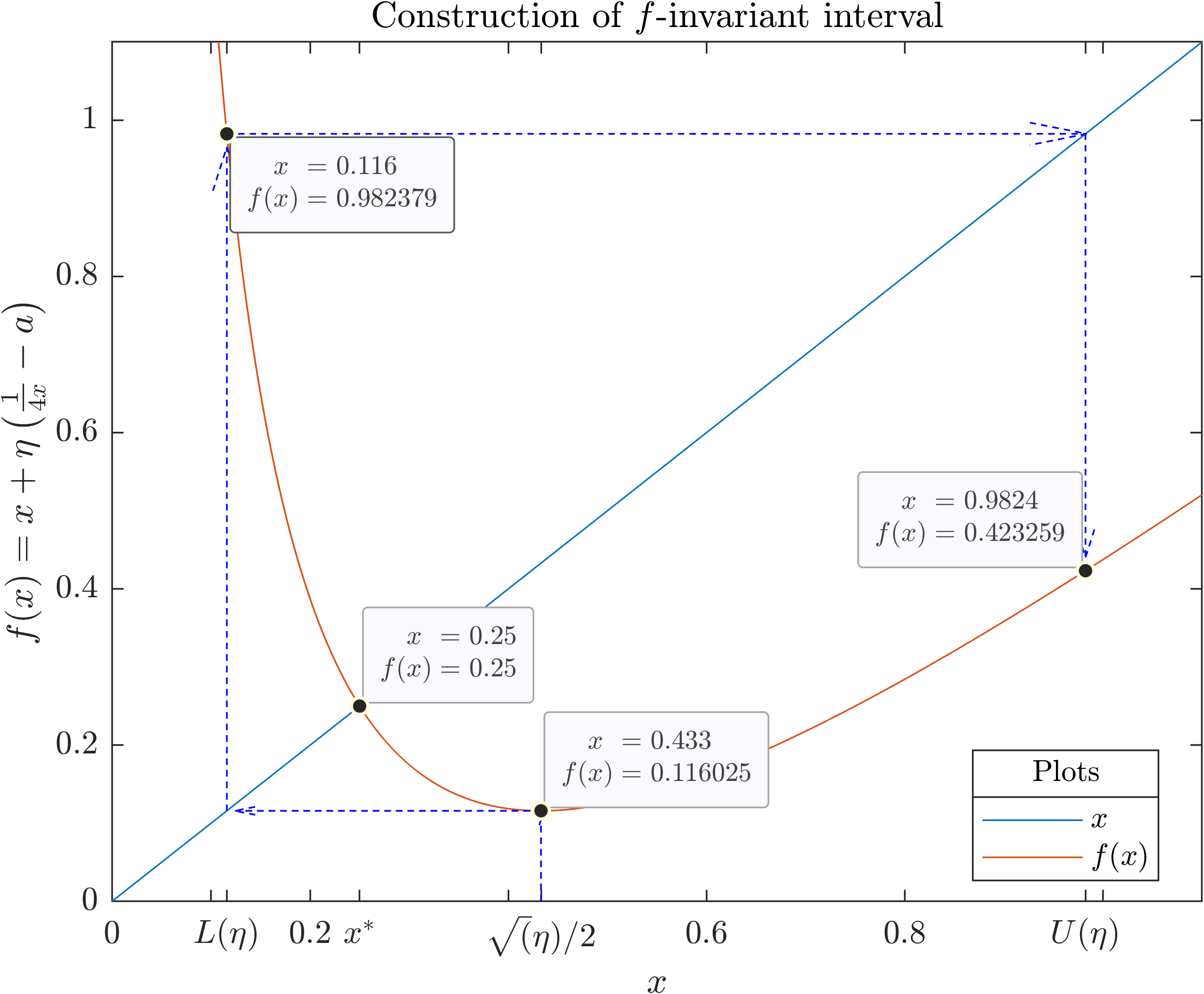
Figure 4: Sketch of the construction of the invariant interval of $f$ for $\alpha=1$ and $\eta=3/4$ in the proof of Lemma 13. Starting from the argmin of $f$ at $x=\sqrt{\eta}/2$ and following the blue dashed arrows, we get the interval $I\left(\eta\right)=[L\left(\eta\right),U\left(\eta\right)]$ with $f\left(I\left(\eta\right)\right)\subseteq I\left(\eta\right)$ and $x^{*}=1/4\alpha\in I\left(\eta\right)$.

Remark.

The selected interval, $\eta\in[3/4\alpha^{2},1/\alpha^{2})$, in the statement of Lemma 13 is not minimal, in the sense that Li-Yorke chaos also appears for values of $\eta$ outside these bounds. However, it is sufficient for our purposes. A sketch of the constructive proof of Lemma 13 is given in Figure 4. In the depicted instantiation, $\alpha=1$ and $\eta=3/4$, yet the image is qualitatively the same for all values of $\eta$ in the above range.

Next, we turn to the existence of a fixed point $p\neq x^{*}\in I\left(\eta\right)$ of $f^{\left(3\right)}\left(x\right):=\left(f\circ f\circ f\right)\left(x\right)$. The result is formally established in Proposition 14, which concludes the two-step proof of Li-Yorke chaos.

Proposition 14.

Let $\alpha\geq 1$ arbitrary and let $f^{\left(3\right)}\left(x\right):=\left(f\circ f\circ f\right)\left(x\right)$. Then, for any $\eta\in\left[3/4\alpha^{2},1/\alpha^{2}\right)$, $f^{\left(3\right)}\left(x\right)$ is continuous for $x>0$ and

$$f^{\left(3\right)}\left(\sqrt{\eta}/2\right)-\sqrt{\eta}/2\geq 0>f^{\left(3\right)}\left(U\left(\eta\right)\right)-U\left(\eta\right),$$

where $U\left(\eta\right)$ is defined in Lemma 13. In particular, $f^{\left(3\right)}\left(x\right)$ has an additional fixed point $p\neq x^{*}=1/4\alpha$ with $p\in\left[\sqrt{\eta}/2,U\left(\eta\right)\right]$.

Proof.

Since $\eta\in\left[3/4\alpha^{2},1/\alpha^{2}\right)$, it will be convenient to parametrize $\eta$ as

$$\eta:=\frac{c}{4\alpha^{2}},\vspace*{0.1in}$$

with $c\in[3,4)$. We present here the proof for $c\in[3+\delta,4)$ for $\delta\approx 0.00918$ which is more intuitive and omit the case $c\in[3,3+\delta)$. The argument is essentially the same for values of $\eta\in[3/4\alpha^{2},(3+\delta)/4\alpha^{2}]$. However, the numerical evaluation of $f^{\left(3\right)}\left(x\right)$ is more involved and is thus omitted. In any case, the exact interval for which existence of an additional fixed point is established does not affect the overall result.

We first prove that $f^{\left(3\right)}\left(\sqrt{\eta}/2\right)-\sqrt{\eta}/2\geq 0$. The proof exploits the fact that $f^{\left(3\right)}\left(x\right)$ is locally maximized at the argmin $x=\sqrt{\eta}/2$ of $f\left(x\right)$. Hence, (using mathematical software), we obtain that

$$f^{\left(3\right)}\left(\sqrt{\eta}/2\right)-\sqrt{\eta}/2=\frac{1}{2\alpha}\cdot\frac{64c^{3/2}+6c^{5/2}-32c^{2}-57c+19\sqrt{c}}{-4c^{3/2}+20c-34\sqrt{c}+20}\,,$$

which can be shown to be increasing in $c$. A visual representation of $f^{\left(3\right)}\left(\sqrt{\eta}/2\right)-\sqrt{\eta}/2$ is given in the left panel of Figure 5. Since equality with zero occurs for $c\approx 3.00918$, it follows that the expression remains positive for $c\in[3.00918,4]$, or equivalently for $\eta\in[3.00918/4\alpha^{2},1/\alpha^{2}]$.

Next, we prove that $f^{\left(3\right)}\left(U\left(\eta\right)\right)-U\left(\eta\right)<0$. Recall by the proof of Lemma 13 that $U\left(\eta\right)=f^{\left(2\right)}\left(\sqrt{\eta}/2\right)$, where $f^{\left(2\right)}\left(x\right):=\left(f\circ f\right)\left(x\right)$. Hence,

$$f^{\left(3\right)}\left(U\left(\eta\right)\right)-U\left(\eta\right)=f^{\left(5\right)}\left(\sqrt{\eta}/2\right)-f^{\left(2\right)}\left(\sqrt{\eta}/2\right)\,,$$

which can be evaluated again by mathematical software. The result is

$$f^{\left(3\right)}\left(U\left(\eta\right)\right)-U\left(\eta\right)=-\frac{1}{2\alpha}\cdot\frac{\left(\sqrt{c}-1\right)^{3}\sqrt{c}\left(-6c^{3/2}+26c-38\sqrt{c}+19\right)^{2}}{\left(2c-6\sqrt{c}+5\right)\left(-34c^{3/2}+6c^{2}+74c-74\sqrt{c}+29\right)}\cdot$$

$$\cdot\frac{\left(-1268c^{3/2}-196c^{5/2}+24c^{3}+677c^{2}+1361c-796\sqrt{c}+199\right)}{\left(-15592c^{3/2}-7486c^{5/2}-536c^{7/2}+48c^{4}+2638c^{3}+13420c^{2}+11490c-4922\sqrt{c}+941\right)}\,.$$

As above, the right hand side can be shown to be decreasing in $c$, cf. right panel of Figure 5. Again, equality with zero occurs $c\approx 3.00918$ and hence the expression remains negative for negative for any $c\in[3.00918,4]$, or equivalently for $\eta\in\left(3.00918/4\alpha^{2},1/\alpha^{2}\right)$. The existence follows from the continuity of $f^{\left(3\right)}\left(x\right)$ in this interval – which can be shown by a standard exercise for values of $\eta<1/\alpha^{2}$ – and the intermediate value theorem. This proves the statement of the Proposition.

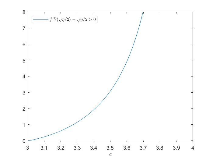
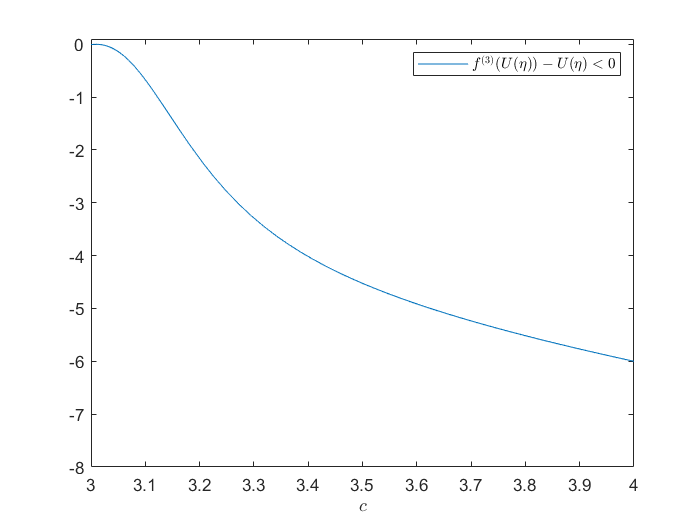
Figure 5: The graphs of $f^{\left(3\right)}\left(\sqrt{\eta}/2\right)-\sqrt{\eta}/2$ (left panel) and $f^{\left(3\right)}\left(U\left(\eta\right)\right)-U\left(\eta\right)$ (right panel) for values of $c[3,4]$ or equivalently for $\eta\in\left[3/4\alpha^{2},1/\alpha^{2}\right)$. The first expression is increasing and remains positive for any $c\geq 3.00918$ and the second expression is decreasing and remains negative for any $c\geq 3.00918$.

∎

The statement of Proposition 14 is illustrated in Figure 6.

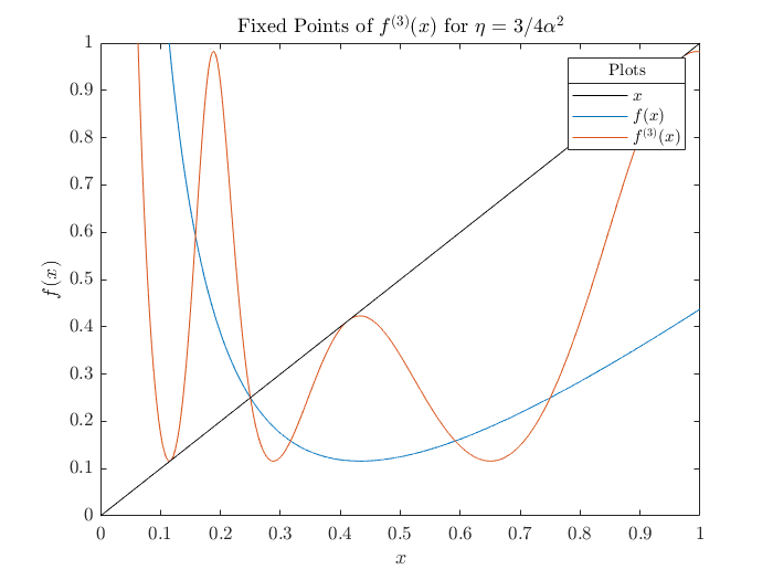
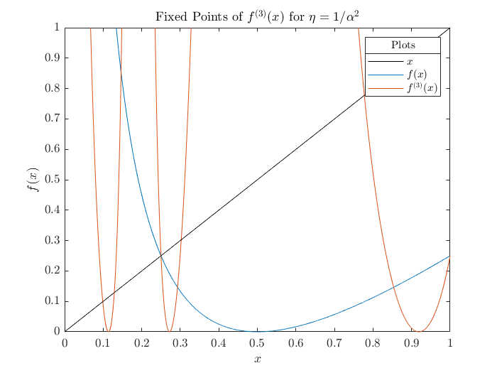
Figure 6: Points of period $3$, i.e., fixed points of the function $f^{\left(3\right)}\left(x\right)=\left(f\circ f\circ f\right)\left(x\right)$ in the interval $\left(0,1\right)$. The plots of $f\left(x\right)$ and $f^{\left(3\right)}\left(x\right)$ have one common fixed point (common intersection point with the diagonal), however $f^{\left(3\right)}\left(x\right)$ has more fixed points. For intermediate cases, i.e., for $3/4\alpha^{2}<\eta<1/\alpha^{2}$, the graph of $f^{\left(3\right)}\left(x\right)$ stretches continuously from the image in the left panel to the image in the right panel. For the illustrations $\alpha=1$, but the outcome is qualitatively equivalent for any choice of $\alpha$ in the admissible range.

C.1 Best Response Dynamics

While the previous technique does not allow us to establish Li-Yorke chaos in the case of Best Response (BR) Dynamics, we complement the existing empirical results of [41] and [50] with a formal proof of the stability properties of the BR dynamics via eigenvalue analysis of a first order linear approximation of the original non-linear system. Due to the first order approximation, the boundary cases are not precise, however, qualitatively, the result is robust. Recall, that for TC with isoelastic demand, the BR dynamics take the form

$$x_{i}^{t+1}\leftarrow\sqrt{x_{-i}^{t}/\alpha_{i}}-x_{-i}^{t},\,\,\text{for }i=1,2\text{ and }t\in\mathbb{N}.$$ (8)

Proposition 15.

Under the Best Response (BR) update rule, (8), the evolution of the sequence $\left(x^{t},y^{t}\right)$ of effort level pairs around the unique equilibrium depends on the value of the ratio $r:=\alpha/\beta$ of the abilities of the two firms relative to the points $r_{0}:=3+2\sqrt{2}$ and $r_{0}^{-1}$

• If $r_{0}^{-1}<r<r_{0}$, the effort levels are spiralling inwards towards the unique equilibrium (stable spiral focus).

• If $r=r_{0}^{-1}$ or $r=r_{0}$, the effort levels cycle around the unique equilibrium effort level (neutral center).

• If $r<r_{0}^{-1}$ or $r>r_{0}$, the effort levels are spiralling outwards away from the unique equilibrium effort level (unstable spiral focus).

An instantiation of the result of Proposition 15 is shown in Figure 7.

Proof.

The unique resting point of the best response dynamics is given by the simultaneous solutions of the equations in equation (8) which yields

$$\left(x^{*},y^{*}\right)=\left(v\beta,v\alpha\right)/\left(\alpha+\beta\right)^{2}.$$

The stability of the dynamical system (8) around the equilibrium $\left(x^{*},y^{*}\right)$ can be determined by the eigenvalues of the Jacobian of the system at the equilibrium point,

$$J =\left.\begin{pmatrix}\frac{\partial}{\partial x}x^{t+1}\left(x,y\right)&\frac{\partial}{\partial y}x^{t+1}\left(x,y\right)\\ \frac{\partial}{\partial x}y^{t+1}\left(x,y\right)&\frac{\partial}{\partial y}y^{t+1}\left(x,y\right)\end{pmatrix}\right|_{\left(x,y\right)=\left(x^{*},y^{*}\right)}=\begin{pmatrix}0&-\frac{1}{2r}\left(r-1\right)\\ \frac{1}{2}\left(r-1\right)&0\end{pmatrix},$$

which yields the characteristic equation

$$\det\left(J-\lambda I\right)=\lambda^{2}+\frac{1}{4r}\left(r-1\right)^{2},$$

and hence, the complex conjugate eigenvalues $\lambda_{1,2}$ with absolute value $|\lambda_{1}|=|\lambda_{2}|=\frac{1}{2\sqrt{r}}|r-1|$. This implies that the dynamics oscillate around the equilibrium with the exact behavior depending on whether the absolute value of $\lambda_{1,2}$ is less than, equal to or larger than $1$. In particular,

$$\frac{1}{2\sqrt{r}}|r-1|=1 \iff r^{2}-6r+1=0\iff\left(r-r_{0}\right)\left(r-r_{0}^{-1}\right)=0,$$

with $r_{0}:=3+2\sqrt{2}$, which concludes the proof. ∎

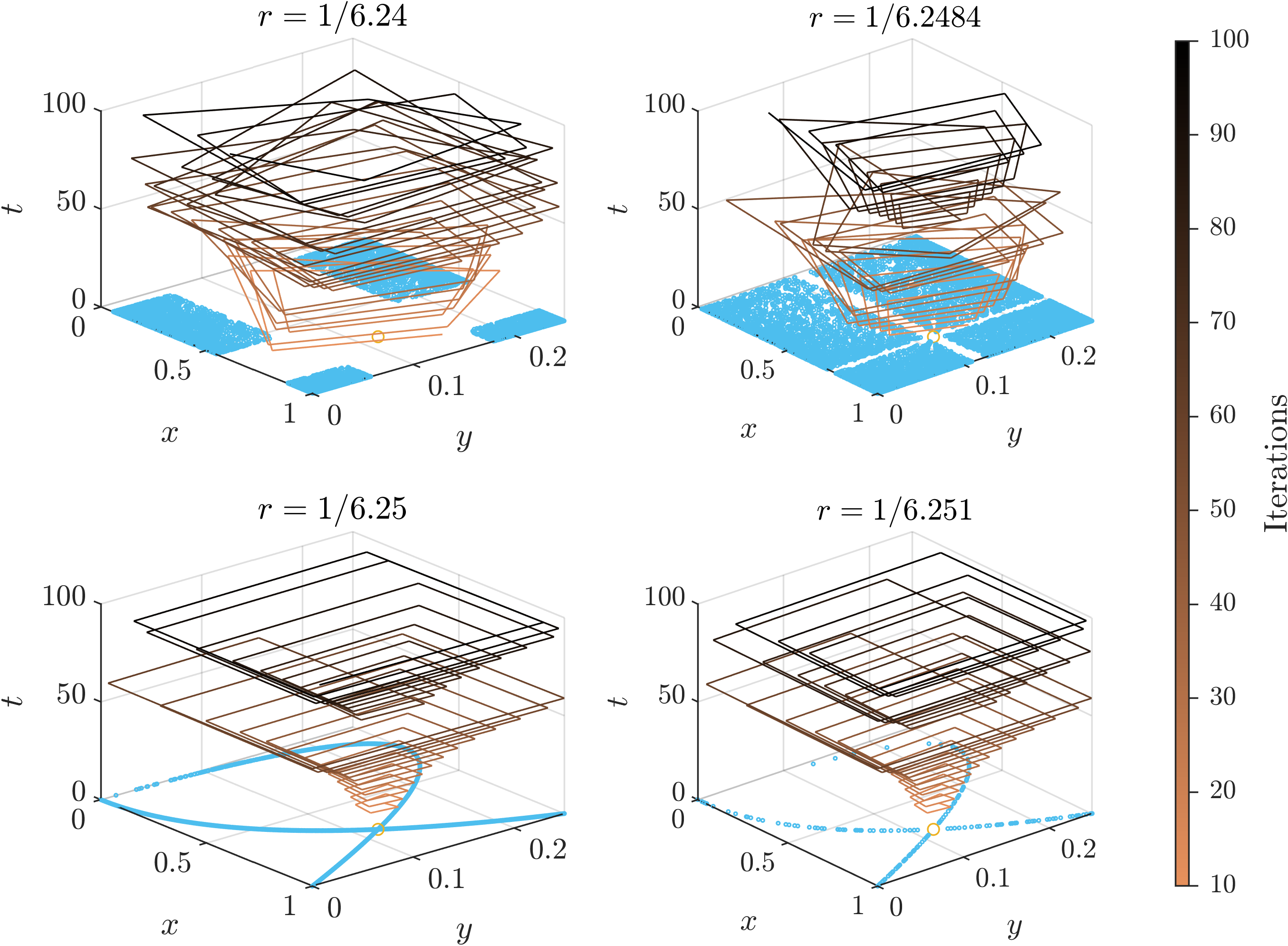
Figure 7: The trajectories (light to dark lines) of outputs $\left(x^{t},y^{t}\right)$ with respect to time $t\in[10,100]$ (vertical axis). The light blue dots denote their projections on the $x-y$ plane for a longer time span $t\in[10^{3},2\cdot 10^{3}]$. While all dynamics spiral away from the unique equilibrium (red circle on the $x-y$ plane) in agreement with Proposition 15, their attractors change significantly for only small perturbations in the parameters of the game as expressed by the asymmetry-ratio $r$.

References

- [1] B. Adsul, Ch. S. Babu, J. Garg, R. Mehta, and M. A. Sohoni. Nash Equilibria in Fisher Market. In 3rd SAGT, pages 30–41, 2010.
- [2] N. Arnosti and S. M. Weinberg. Bitcoin: A Natural Oligopoly. In Avrim Blum, editor, 10th ITCS, volume 124, pages 5:1–5:1, 2018.
- [3] Moshe Babaioff, Brendan Lucier, Noam Nisan, and Renato Paes Leme. On the efficiency of the walrasian mechanism. In ACM Conference on Economics and Computation, EC ’14, pages 783–800, 2014.
- [4] J. Bielawski, T. Chotibut, F. Falniowski, G. Kosiorowski, M. Misiurewicz, and G. Piliouras. Follow the Regularized Leader Routes to Chaos in Routing Games. arXiv e-prints, page arXiv:2102.07974, February 2021.
- [5] B. Birnbaum, N. R. Devanur, and L. Xiao. Distributed Algorithms via Gradient Descent for Fisher Markets. In EC’11, pages 127–136. ACM, 2011.
- [6] G. Bissias, B. N. Levine, and D. Thibodeau. Greedy but Cautious: Conditions for Miner Convergence to Resource Allocation Equilibrium, 2019.
- [7] S. Boyd and L. Vandenberghe. Convex Optimization. Cambridge University Press, New York, NY, USA, 2004.
- [8] S. Brânzei, Y. Chen, X. Deng, A. Filos-Ratsikas, S.K.S. Frederiksen, and J. Zhang. The Fisher Market Game: Equilibrium and Welfare. In 28th AAAI, pages 587–593, 2014.
- [9] S. Brânzei, N. R. Devanur, and Y. Rabani. Proportional Dynamics in Exchange Economies. CoRR, abs/1907.05037, 2019.
- [10] S. Brânzei, R. Mehta, and N. Nisan. Universal Growth in Production Economies. In NeurIPS 2018, volume 31, pages 1973–1973, 2018.
- [11] G. Chen and M. Teboulle. Convergence Analysis of a Proximal-Like Minimization Algorithm Using Bregman Functions. SIAM J. Optim., 3(3):538–543, 1993.
- [12] Ning Chen, Xiaotie Deng, Hongyang Zhang, and Jie Zhang. Incentive ratios of fisher markets. In Automata, Languages, and Programming - 39th International Colloquium, ICALP 2012, pages 464–475, 2012.
- [13] Ning Chen, Xiaotie Deng, and Jie Zhang. How profitable are strategic behaviors in a market? In Algorithms - ESA 2011 - 19th Annual European Symposium, pages 106–118, 2011.
- [14] X. Chen, C. Papadimitriou, and T. Roughgarden. An Axiomatic Approach to Block Rewards. In Proceedings of the 1st ACM Conference on Advances in Financial Technologies, AFT ’19, pages 124–131, New York, NY, USA, 2019. ACM.
- [15] Y. K. Cheung, R. Cole, and N. R. Devanur. Tatonnement beyond gross substitutes? Gradient descent to the rescue. Games and Economic Behavior, 123:295–326, 2020.
- [16] Y. K. Cheung, R. Cole, and A. Rastogi. Tatonnement in ongoing markets of complementary goods. In EC’12, pages 337–354, 2012.
- [17] Y. K. Cheung, R. Cole, and Y. Tao. Dynamics of Distributed Updating in Fisher Markets. In EC’18, pages 351–368, 2018.
- [18] Y. K. Cheung, M. Hoefer, and P. Nakhe. Tracing equilibrium in dynamic markets via distributed adaptation. In AAMAS, pages 1225–1233, 2019.
- [19] Y. K. Cheung and G. Piliouras. Vortices Instead of Equilibria in MinMax Optimization: Chaos and Butterfly Effects of Online Learning in Zero-Sum Games. In COLT, pages 807–834, 2019.
- [20] Y. K. Cheung and G. Piliouras. Chaos, Extremism and Optimism: Volume Analysis of Learning in Games. In NeurIPS (Pre-proceedings), 2020.
- [21] Y. K. Cheung and Y. Tao. Chaos of Learning Beyond Zero-Sum and Coordination via Game Decompositions. In ICLR, 2021.
- [22] T. Chotibut, F. Falniowski, M. Misiurewicz, and G. Piliouras. Family of chaotic maps from game theory. Dynamical Systems, pages 1–16, 2020. Published online.
- [23] T. Chotibut, F. Falniowski, M. Misiurewicz, and G. Piliouras. The route to chaos in routing games: When is Price of Anarchy too optimistic? In H. Larochelle, M. Ranzato, R. Hadsell, M. F. Balcan, and H. Lin, editors, Advances in Neural Information Processing Systems, volume 33, pages 766–777. Curran Associates, Inc., 2020.
- [24] R. Cole, N. R. Devanur, V. Gkatzelis, K. Jain, T. Mai, V. V. Vazirani, and S. Yazdanbod. Convex Program Duality, Fisher Markets, and Nash Social Welfare. In EC’17, pages 459–460, 2017.
- [25] R. Cole and Y. Tao. Large Market Games with Near Optimal Efficiency. In EC’16, pages 791–808, New York, NY, USA, 2016. ACM.
- [26] A. A. Cournot. Recherches sur les principes mathematiques de la theorie des richesses / Pref. de Henri Guitton. Hachette Paris, 1838.
- [27] N. R. Devanur. Fisher Markets and Convex Programs. Unpublished manuscript, 2009.
- [28] D. DiPalantino and M. Vojnovic. Crowdsourcing and All-Pay Auctions. In EC ’09, pages 119–128, 2009.
- [29] E. Eisenberg. Aggregation of utility functions. Management Sciences, 7(4):337–350, 1961.
- [30] E. Eisenberg and D. Gale. Consensus of Subjective Probabilities: The Pari-Mutuel Method. Ann. Math. Statist., 30(1):165–168, 1959.
- [31] A. Fiat, A. Karlin, E. Koutsoupias, and C. Papadimitriou. Energy Equilibria in Proof-of-Work Mining. In EC’19, pages 489–502, 2019.
- [32] T. Galla and J. D. Farmer. Complex Dynamics in Learning Complicated Games. PNAS, 110(4):1232–1236, 2013.
- [33] G. Goren and A. Spiegelman. Mind the Mining. In EC ’19, pages 475–487, 2019.
- [34] J. J. Horton and L. B. Chilton. The Labor Economics of Paid Crowdsourcing. In Proceedings of the 11th ACM Conference on Electronic Commerce, EC ’10, pages 209–218, 2010.
- [35] S. Leonardos, B. Monnot, D. Reijsbergen, S. Skoulakis, and G. Piliouras. Dynamical Analysis of the EIP-1559 Ethereum Fee Market. arXiv e-prints, page arXiv:2102.10567, February 2021.
- [36] D. Levin, K. LaCurts, N. Spring, and B. Bhattacharjee. Bittorrent is an Auction: Analyzing and Improving Bittorrent’s Incentives. SIGCOMM Comput. Commun. Rev., 38(4):243–254, 2008.
- [37] T.-Y. Li and J. A. Yorke. Period Three Implies Chaos. The American Mathematical Monthly, 82(10):985–992, 1975.
- [38] Á. L. López and X. Vives. Overlapping Ownership, R&D Spillovers, and Antitrust Policy. Journal of Political Economy, 127(5):2394–2437, 2019.
- [39] John Nash. Non-cooperative games. Annals of Mathematics, 54(2):286–295, 1951.
- [40] G. Palaiopanos, I. Panageas, and G. Piliouras. Multiplicative Weights Update with Constant Step-Size in Congestion Games: Convergence, Limit Cycles and Chaos. In NIPS’17, pages 5874–5884, 2017.
- [41] T. Puu. Chaos in duopoly pricing. Chaos, Solitons & Fractals, 1(6):573–581, 1991.
- [42] Y. Sato, E. Akiyama, and J. D. Farmer. Chaos in Learning a Simple Two-person Game. PNAS, 99(7):4748–4751, 2002.
- [43] B. Skyrms. Chaos in game dynamics. Journal of Logic, Language and Information, 1(2):111–130, 1992.
- [44] F. Szidarovszky and K. Okuguchi. On the Existence and Uniqueness of Pure Nash Equilibrium in Rent-Seeking Games. Games and Economic Behavior, 18(1):135–140, 1997.
- [45] R. D. Theocharis. On the Stability of the Cournot Solution on the Oligopoly Problem1. The Review of Economic Studies, 27(2):133–134, 02 1960.
- [46] G. Tullock. Efficient Rent Seeking. In J. Buchanan, R. Tollison, and G. Tullock, editors, Toward a Theory of Rent Seeking Society, pages 97–112. Texas A&M University Press, College Station, 1980.
- [47] H. R. Varian. Intermediate Microeconomics: A Modern Approach. W.W. Norton & Co., New York, eighth edition, 2010.
- [48] John Von Neumann. A model of general economic equilibrium. In F. H. Hahn, editor, Readings in the Theory of Growth: a selection of papers from the Review of Economic Studies, pages 1–9. Palgrave Macmillan UK, London, 1971.
- [49] L. Walras. Éléments d’économie politique pure ou théorie de la richesse sociale (Elements of Pure Economics, or the theory of social wealth). Lausanne, Paris, 1874. (1899, 4th ed.; 1926, rev ed., 1954, Engl. transl.).
- [50] K. Wärneryd. Chaotic dynamics in contests. Economic Inquiry, 56(3):1486–1491, 2018.
- [51] F. Wu and L. Zhang. Proportional Response Dynamics Leads to Market Equilibrium. In STOC ’07, pages 354–363, 2007.
- [52] L. Zhang. Proportional response dynamics in the Fisher market. Theor. Comput. Sci., 412(24):2691–2698, 2011.