JUNO sensitivity to low energy atmospheric neutrino spectra
Abstract
Atmospheric neutrinos are one of the most relevant natural neutrino sources that can be exploited to infer properties about cosmic rays and neutrino oscillations. The Jiangmen Underground Neutrino Observatory (JUNO) experiment, a 20 kton liquid scintillator detector with excellent energy resolution is currently under construction in China. JUNO will be able to detect several atmospheric neutrinos per day given the large volume. A study on the JUNO detection and reconstruction capabilities of atmospheric and fluxes is presented in this paper. In this study, a sample of atmospheric neutrino Monte Carlo events has been generated, starting from theoretical models, and then processed by the detector simulation. The excellent timing resolution of the 3” PMT light detection system of JUNO detector and the much higher light yield for scintillation over Cherenkov allow to measure the time structure of the scintillation light with very high precision. Since and interactions produce a slightly different light pattern, the different time evolution of light allows to discriminate the flavor of primary neutrinos. A probabilistic unfolding method has been used, in order to infer the primary neutrino energy spectrum from the detector experimental observables. The simulated spectrum has been reconstructed between 100 MeV and 10 GeV, showing a great potential of the detector in the atmospheric low energy region.
1 Introduction
Atmospheric neutrinos are a naturally occurring neutrino source. They originate from the decays of and produced in extensive air showers initiated by the interaction of cosmic rays with the Earth’s atmosphere [1, 2, 3, 4]. The energy spectrum of primary cosmic rays above 100 MeV can be described by a power law , where the spectral index is for GeV and above that value [5]. At energies larger than GeV, the spectrum becomes steeper ()[6] and it flattens again when GeV. In the interaction of a single high energy Cosmic Ray with the nuclei of the Earth’s atmosphere, hundreds or thousands mesons can be produced. The atmospheric neutrino energy spectrum spans a wide range from the MeV up to the PeV scale and can be roughly described by a power law [7, 8, 9, 10, 11]. The spectral index is, in general, steeper than that of primary cosmic rays, since the parent mesons lose a large fraction of their energy before decaying. The spectrum intensity is suppressed at sub–GeV energies reflecting the rigidity cutoff, that describes the shielding provided by the geomagnetic field against the arrival of cosmic rays particles from outside the magnetosphere. Neutrinos originating from muon decays contribute mainly up to a few GeV. The flavor ratio (+)/(+) is around two at 1 GeV and increases as the energy increases, since more muons are likely to reach the Earth’s surface without decaying. At energies above hundreds of GeV, the decay length of and becomes longer than their path length in the atmosphere, leading to a neutrino flux reduction. At the highest energies, the decay of heavy charmed mesons is expected to dominate the atmospheric neutrino production. Given the very short lifetime of these particles, the associated neutrino flux is commonly referred as “prompt” [12, 13, 14].
Since the Earth is mostly transparent to neutrinos below the PeV energy scale, an atmospheric neutrino detector is able to see neutrinos coming from all directions. The distance from the production point to the detector varies from to km, depending on the zenith angle [15]. The angular distribution has a characteristic shape with an increased flux towards the horizontal direction (with respect to the vertical direction), due to the longer path length of parent particles in the atmosphere. In the sub–GeV energy region there is an asymmetry along the East–West axis, which reflects the azimuthal dependence of the rigidity cutoff of the cosmic rays.
Atmospheric neutrinos were detected for the first time in the 1960s [16, 17]. Further measurements led to the discovery of neutrino flavor oscillations in 1998 [18]. Some of the missing pieces in the puzzle of neutrino physics are going to be addressed also by means of atmospheric neutrinos. The field of research is currently very active and several experiments are scheduled in the coming years to answer the unsolved questions. Next-generation detectors for atmospheric neutrino physics plan to significantly improve performances, compared to present ones, by increasing their size and detection granularity. The efforts are mostly concentrated on flavor oscillation physics, pushing the detectors sensitivity for the neutrino mass ordering (MO) and the CP phase in the neutrino sector. The most prominent examples are DUNE [19], Hyper-Kamiokande [20], INO [21], ORCA [22], and PINGU [23].
In Figure 1, present measurements of the energy spectrum of atmospheric neutrinos are reported, including predictions from theoretical models.
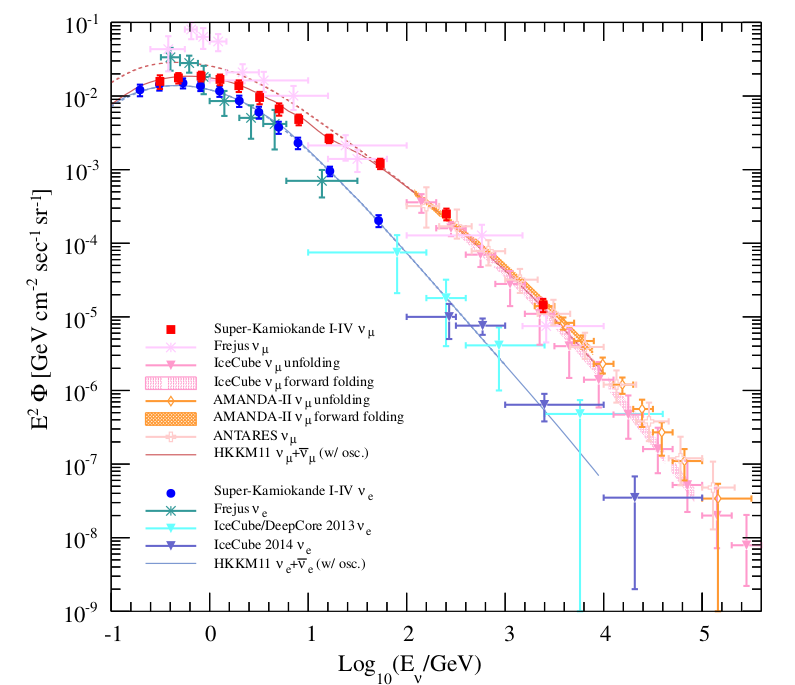
Measurements performed over the last decades, up to present times, are able to cover a very wide range in the neutrino energy, from several hundreds of MeV to several hundreds of TeV. This sector has been explored predominantly by Cherenkov detectors, such as Super-Kamiokande [7] and IceCube [8, 9, 10, 24]. The Jiangmen Underground Neutrino Observatory (JUNO), currently under construction in China, will be able to detect several atmospheric neutrinos per day. JUNO is going to become the largest liquid scintillator (LS) based detector ever built, having a target LS mass more than one order of magnitude larger than present ones. The large detector mass is one of the key-points for atmospheric neutrino detection, since it is comparable to the largest present water-based detector, Super-Kamiokande. Despite the limited ability of JUNO in tracking single particles after a neutrino interaction, with respect to large Cherenkov detectors, and a slightly reduced accessible statistics, the LS nature of the detector allows more precise measurements towards the low energy region. This sector of the energy spectrum is still not fully covered by present and past experiments. Furthermore, it also corresponds to the region where theoretical models have the largest uncertainties.
The atmospheric neutrino flux measurements by means of the JUNO detector allow to investigate the neutrino MO and the octant. It is possible to pursue also the CP phase measurement. In our work, we investigate JUNO’s potential for measuring the atmospheric and fluxes in the energy range 100 MeV – 10 GeV.
2 JUNO experiment
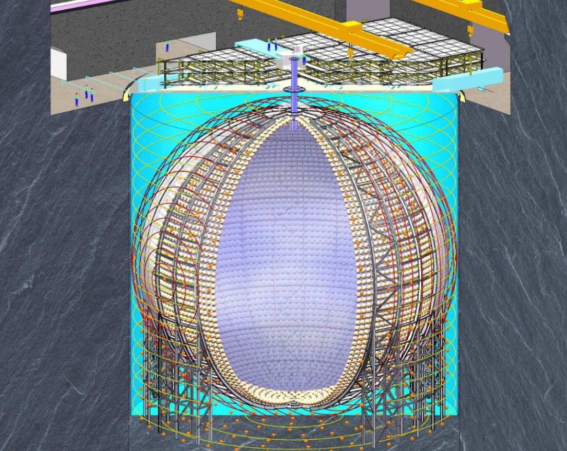
The JUNO experiment [25, 26] is a LS neutrino detector currently under construction in a dedicated underground laboratory (about 700 m deep, 1800 m.w.e.) near Kaiping, Jiangmen city, Guandong province (P. R. China). A sketch of the detector is shown in Figure 2. The central detector (CD) consists of 20 kton of LS, contained in a 12 cm thick, highly transparent, acrylic sphere with a diameter of 35.4 m. The light produced in the LS is read out by 17612 20” high quantum efficiency (QE) photomultiplier tubes (PMTs) and 25600 3” PMTs, providing a total photo–coverage of more than 75%. About 13000 of the 20” PMTs are Microchannel Plate (MCP) PMTs, developed by the JUNO collaboration and currently being produced by the North Night Vision Technology company. The remaining 5000 20” PMTs consist of the R12860 model produced by Hamamatsu. Both of these PMTs have a photon detection efficiency greater than 27%. For the 20” PMTs, the full waveform will be acquired. Their large photon collection area, however, has the consequence of a large dark noise rate, on average of the order of 30 kHz, and a time resolution on single photo-electrons in the range from 1 ns to 10 ns. The additional 3” PMTs, built by the HZC company, are deployed in the 20” PMTs’ lattice structure, in order to reduce any possible systematics due to the loss of linearity in charge reconstruction and to improve the timing measurements [27]. Due to their small area, the 3” PMTs will operate in digital mode, thus being an independent readout system that can be exploited for cross-calibrating the 20” PMTs energy response. This feature becomes extremely important for high-energy events, where millions of photons are produced. Furthermore, due to the size difference, the Transit Time Spread (TTS) of 3” PMTs is of the order of the nanosecond, while the 20” PMTs one is larger, on average.
The acrylic sphere is surrounded by a stainless steel truss structure, which has a diameter of about 40 m and constitutes the mechanical support for both the acrylic sphere and the PMTs. The central detector is submerged in a 44 m deep water pool (WP) filled with 30 kton of ultrapure water and instrumented with 2400 20” MCP-PMTs. It acts as an active Cherenkov muon veto and shields the CD against external radioactivity. The walls of the pool are covered with high–reflectivity Tyvek film, in order to increase the photon collection and allowing to veto Cosmic Ray muons with 95% efficiency. A Top Tracker (TT) is placed on top of the water pool, to improve the total veto efficiency and the reconstruction of atmospheric muons. The TT consists of three layers of scintillator strip detectors, refurbished after the decommissioning of the OPERA experiment Target Tracker [28]. It has a granularity of cm2 and a coverage of about 60% of the WP top surface.
The JUNO LS mixture consists of three components: Linear Alkylbenzene (LAB) as solvent, 2.5 g/l of 2,5-Diphenyloxazole (PPO) as scintillation fluor and 3 mg/l of 1,4–Bis(2–methylsyryl) benzene (bis–MSB) as wavelength shifter [29]. This mixture ensures an effective light yield of photons per MeV of deposited energy and an attenuation length greater than 20 m for 430 nm photons. The designed radio-purity levels of the JUNO LS are g/g for the bulk 238U, 232Th, and 40K contaminants [30]. The calibration of the JUNO CD will be performed by four different systems [31]. An Automated Calibration Unit (ACU) will deploy different radioactive sources along the detector vertical axis. The ACU system is also designed to deploy a laser source, with a photon intensity that can cover a range from hundreds of keV up to (TeV) equivalent energy. Two Cable Loop Systems (CLS) will instead place sources across two planes. A guide tube (GT) system, installed on the outer circumference of the sphere, will provide information regarding non-uniformity at the CD boundary. A Remote Operated Vehicle (ROV) will finally deploy sources in the whole detector volume. Periodical calibration campaigns will ensure to keep the overall energy resolution around 3%/ in the MeV energy region, where the analysis for the neutrino MO will focus. Atmospheric neutrinos interacting inside JUNO can produce different final states, depending on the nature of the interaction they undergo. A first distinction can be done between charged-current (CC) and neutral-current (NC) interactions. In the first case, the lepton of the same flavor of the interacting neutrino is produced and therefore the original neutrino information is preserved. In NC interactions, on the contrary, only a hadronic state is visible and the flavor of the interacting neutrino cannot be inferred. In the energy of interest for atmospheric neutrinos, the dominant interaction is the neutrino-nucleon scattering. The most prominent channels are the elastic and quasi-elastic scattering, the resonant production, and the deep inelastic scattering [32]. This last classification concerns only about the final hadronic products, which give information about the original energy of the neutrino, but are not sensitive to the interaction flavor. Instead, the CC or the NC nature of the neutrino interaction implies a fundamental difference in the visible products. Apart from the flavor information, the absence of the flavor-corresponding lepton in the final state for NC interactions means also that the neutrino carries away part of its initial energy, which is not released inside the detector. NC events are therefore expected to be concentrated at lower values of the visible energy, while CC ones dominate at higher energy.
3 Monte Carlo dataset
The study of the atmospheric neutrino flux is usually based on the predictions of the expected flux made by Monte Carlo simulations. In this work, we consider the predictions from the latest version of the HKKM model [33], which we refer to as HKKM14 hereafter. The model assumes a Cosmic Ray spectrum based on BESS [34, 35] and AMS-01 [36] measurements. The DPMJET-III [37] and the JAM [38] hadronic interaction models are used for the simulation of the interaction with the Earth’s atmosphere. The HKKM model provides the calculation of the expected atmospheric neutrino flux at different locations, taking into account the latitude and longitude of the detector. The energy range spans from 100 MeV up to 10 TeV. Solar modulation and the asymmetry in the azimuthal distribution are also considered. In the HKKM parametrization, the neutrino flux is calculated at the source and therefore no oscillation effects are included. The HKKM14 atmospheric neutrino flux prediction, calculated at the JUNO experimental site, is shown in Figure 3. Hereafter, and will be used to label both neutrinos and antineutrinos of electron and muon flavor, respectively.
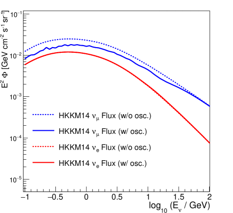
In order to get a realistic prediction, neutrino oscillations have been applied to the original flux, including matter effects. The impact of the oscillation effects has been evaluated according to the standard 3-neutrinos mixing scheme [39].
The interaction of atmospheric neutrinos with the JUNO detector has been simulated by means of the GENIE Neutrino Monte Carlo Generator [40, 41] inside an energy range up to 20 GeV. The elemental composition of the neutrino target has been set as the one of the JUNO LS (mainly 12C and 1H, with relative composition of 0.88 and 0.12, respectively). The output of the simulation contains information about the type of interaction that neutrinos undergo, either a CC or a NC one, and the full list of secondary particles and their associated properties (Particle ID, momentum, direction, ). The contribution of CC interactions has been found not to affect the analysis results by independent evaluations and have been therefore not considered in the present work. Secondary particles produced in the interaction between neutrinos and the JUNO target material have been propagated in the detector by using a GEANT4-based Monte Carlo simulation. The JUNO detector simulation code has been developed within the SNiPER framework [42]. In the detector simulation, several physical processes are included: electromagnetic interaction, decay, hadronic elastic and inelastic interactions, scintillation (including re-emission), Cherenkov emission, and optical absorption. A detailed optical model, including the optical properties of all the detector materials, is also implemented. The output relevant for the analysis includes the timestamp, the number of photoelectrons, and the position of each PMT hit. A data sample of about events have been generated, hereafter called large data sample, in order to set up the procedure used to reconstruct the atmospheric neutrino spectrum and to understand the detector response over a large statistics of events. A sample of 6500 events have been injected in the simulation as a separate Monte Carlo data sample, corresponding to a detector live time of about 5 years. This smaller data sample is hereafter identified as small data sample.
4 Analysis strategy
As a large LS detector, JUNO achieves its best performance on events which are Fully–Contained within the volume, where a calorimetric measurement can be performed. Partially–Contained events, having some secondaries escaping from the CD active volume, are reconstructed with a worse energy resolution. This analysis therefore targets fully–contained events, to be accounted for reconstruction. This sets an intrinsic upper limit of 10 GeV on the flux, since the high–energy muons produced in a CC interaction always escape the CD volume. For (), the “golden” events consist of () fully–contained and CC events and the components to reduce are partially–contained and NC events of all flavor neutrinos. Through–going muons, that may be produced in interactions with materials surrounding the CD, are not considered in this study.
4.1 Fiducial cuts
Before applying the analysis selection to isolate and populations, some preliminary cuts are applied to the large neutrino sample, with the aim of removing low–quality events. A first cut on the interaction vertex position is applied, in order to remove events which release their energy near the edge of the acrylic sphere. These events typically exhibit a loss of linearity between the deposited and the collected energy, because part of the energy is released in the acrylic and water and not in the LS and because the closest PMTs collect a great amount of light and can undergo saturation. A Gaussian smearing with = 1 m has been applied to the MC interaction point (hereafter called vertex), in order to reproduce the uncertainty on the reconstructed position. We require that (i.e. the distance between the vertex and the center of the detector) is less than 16 m to ensure a linear detector response. The precision in the reconstruction vertex at lower energy (in the MeV range) is in general much better than 1 m; on the contrary, at the GeV energy scale, secondary particles can deposit their energy on a long track and the events can no longer be considered as point-like. It has been checked that even an error of few meters on the vertex position does not affect the performance of the selection procedure.
As described in Section 2, the CD is surrounded by a water Cherenkov detector acting as veto for atmospheric muons. Both muons and secondaries coming from partially–contained neutrino events can release a certain amount of energy in the WP and produce a large amount of Cherenkov photons. Therefore, in order to remove partially–contained neutrino events and suppress the atmospheric muon background, we require the total number of hits seen by the water pool veto PMTs to be less than 50, including the contribution from PMT dark noise. This latter term can become important for WP PMTs, because the single-count rate due to WP PMTs dark noise is high (up to several tens of kHz) and the total number of prompt hits from muons Cherenkov light can be small. Hits on WP PMTs are considered in a 200 ns time window, which is approximately the time needed by a muon to cross the entire detector. The dark hits contribution is simulated on a statistical basis, assuming a binomial distribution.
After applying the fiducial cuts described previously, the simulated large neutrino sample is composed at 97% of fully–contained event. The remaining partially–contained events are composed at 96% of CC interactions. The total efficiency for all events is 68%, for events is 63%.
4.2 Atmospheric muon background
The atmospheric muon background consists of the secondary muon flux produced after the interaction of cosmic rays with the atmosphere, in the same way as for neutrinos. The JUNO detector location is about 700 m underground, therefore part of the muon radiation is able to penetrate the rock overburden and release energy inside the detector. The energy released by atmospheric muons inside JUNO is comparable with that of particles coming from atmospheric neutrino interactions (hundreds of MeV - several GeV). Muons can mimic the topology of atmospheric neutrino events and can therefore be a source of background. Although the external water Cherenkov veto is designed to reject these events with high efficiency, the atmospheric muon event rate is several orders of magnitude higher than that from atmospheric neutrino interactions. From preliminary calculations, their event rate inside the JUNO CD is around 3 - 4 Hz, corresponding to roughly times the atmospheric neutrino event rate, considering that the average energy of atmospheric muons reaching JUNO is 207 GeV. The desired acceptance rate for the atmospheric muon background must be therefore at least of the order of . In order to get a comprehensive picture of the atmospheric muon flux within the framework of this study, a full MC simulation is necessary. Atmospheric muons produce several millions of photons in the JUNO LS and the full detector simulation requires high CPU power and storage. For this purpose, a sample of only muon events has been generated, according to the energy and angular distributions evaluated at the JUNO site. The expected muon flux in the detector is calculated within the JUNO Collaboration according to a parametrized model at Earth surface [43] and simulating muons propagation through matter [44]. A detector simulation has been performed. Atmospheric muons in JUNO appear as high-energy tracks which release a large amount of energy both in the WP and in the CD. The fiducial cuts described in Section 4.1 require instead a low collected light inside the WP.
Hereafter, the readout charge of the event, in terms of the number of PEs collected by CD 20” PMTs, is called NPE. NPE represents the observable used to reconstruct the neutrino energy. The same fiducial cuts have been applied to the muon sample, with the additional request of more than NPE, which is the region of interest for the analysis. An acceptance of at 90% confidence level is achieved. The accuracy in the estimation of the acceptance will be improved by increasing the Monte Carlo statistics.
4.3 Neutrino flavor identification
As mentioned above, () CC interactions are the preferred detection channels, since the corresponding charged leptons have very different behaviours. Electrons lose energy quickly via bremsstrahlung and ionization and even at GeV energies their track length is no more than 1-2 meters. On the contrary, muons with energy greater than 1 GeV have longer tracks inside the detector volume. Low–energy muons, moreover, may decay inside the scintillator volume and give a delayed energy release from the Michel electron. The above differences make CC events more extended in time and space, with respect to CC events. The latter component has indeed a much shorter evolution. Hadronic particles are common to all classes of events and make up the visible part of NC events. Hadrons, in general, have a long energy release, because of their interactions and decays.
The event time profile can be therefore exploited to discriminate between different classes of events [45]. A high–precision measurement of the photon arrival time is an important requirement. For this reason, the timing information is taken from the data of the 3” PMT system of the JUNO detector, which have a low TTS value. A Gaussian smearing with a typical width ns (taken from preliminary measurements) has been applied to the true Monte Carlo hit time over each 3” PMT. In order to be aligned to a realistic DAQ window, only events inside a 1.2 time window have been considered. A time residual is then defined for each hit on the i–th 3” PMT as:
| (1) |
where is the hit time on the i–th 3” PMT, is the refraction index of the JUNO liquid scintillator and is the distance between the reconstructed vertex position and the i–th 3” PMT. The time profile of the scintillation light emitted by and CC events is different and the latter has a more prominent tail; therefore, the RMS of the distribution - hereafter called - over the fired 3” PMTs can be used as discrimination parameter. In Figure 4, the distribution is reported for the three populations: CC, CC, and NC events. The variable is also reported separately in 4 different intervals of NPE, selected such as to have equal statistics in each of them.
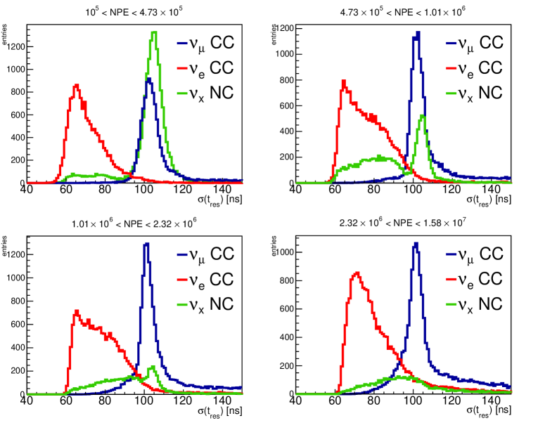
The plots in Figure 4 show a good separation between the CC and the CC component, over the whole energy range. The NC component appears to be overlapped mainly to CC events, with a tail also in the CC region. The reason is that a large fraction of the hadronic component of the secondaries is made of pions, that either decay to + () or to two gammas (). The first category is almost indistinguishable from CC events, while the second one results in electromagnetic showers and resembles the CC component. The relative weight of charged and neutral pions in the final state changes across the energy, as well as that of nucleons. This feature is at the origin of the different shape of the distribution for NC events in Figure 4, since each of the four bins of NPE corresponds to a different energy interval. Protons and neutrons, moreover, have a time profile similar to the one of muons, because they result in a long-lasting energy release inside the LS. The contribution of NC component, however, becomes less significant at high energy, due to its steeper spectral shape. In NC events, indeed, part of the initial energy of the interacting neutrino is carried away by the neutrino itself and is not deposited inside the detector. Given the different features, two separate selection criteria are used to maximize CC events. In order to separate events, a value of < 75 ns is required. The cut results in an efficiency for events 42%, with respect to the large sample after fiducial cuts, and a residual contamination from less than 6%. A requirement of > 95 ns is required to isolate events. In order to reduce the contribution from NC events at low energy, an additional requirement of NPE has been set for selection, thus limiting the analysis to events with a neutrino energy 400 MeV. The efficiency for events is 85% with respect to the large sample after fiducial cuts and the residual contamination is less than 20%. The residual NC events are populated both by and .
The flavor identification procedure has been extensively checked by means of an independent analysis. A variation of the cut has been applied and the resulting efficiency and contamination are in a very good agreement within the statistical and systematic errors reported in this work.
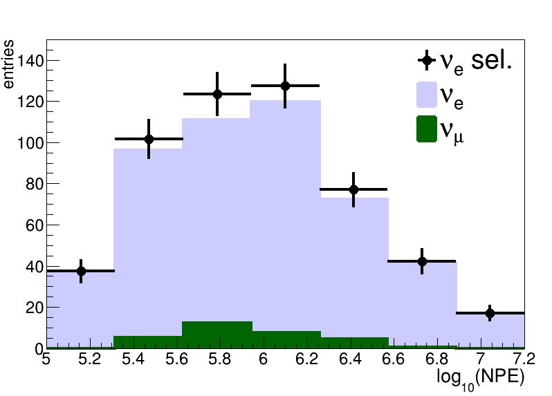
In order to test the JUNO performance in reconstructing the atmospheric neutrino flux, we used the small Monte Carlo sample corresponding to 5 years of data-taking described in Section 3. The energy range considered for the atmospheric flux is , expressed in units and is divided in seven bins. The corresponding (NPE) range is , divided in seven bins as well. Similarly, the energy range for is , divided in seven bins, and the corresponding (NPE) range is , divided in eight bins. The distribution of (NPE) is reported in Figure 5, in the bins used in the analysis. A summary of the small sample population is in Table 1, as a function of the flavor and of the cuts applied, in the NPE regions considered.

| Events injected in the simulation | 6500 | |
| Charge region | 1725 | 1241 |
| Fiducial cuts | 1167 | 773 |
| cut | 495 | 661 |
| Residual background | 30 | 163 |
4.4 Unfolding
The determination of the atmospheric neutrino energy spectrum, starting from the detector experimental observables, is a classical unfolding problem. In this case, the true spectrum is deconvolved from the distribution of the experimental observables, knowing the detector response. In the classical fitting method, on the other hand, the true distribution is extracted from the observables by directly comparing the experimental distribution with the results of a model prediction. The main benefit of the unfolding is that it does not require a particular choice of the spectrum parametrization. In a liquid scintillator detector like JUNO, the main observable for the energy reconstruction is the total number of photoelectrons NPE detected by the 20” PMTs. This value is related to the total energy deposit in the LS and therefore to the neutrino energy. The neutrino energy spectrum is then unfolded from the NPE spectrum. In general, the observable NPE spectrum can be expressed in terms of the primary neutrino spectrum as
| (2) |
where is the likelihood matrix, which can be estimated by means of a full detector simulation. The relationship in Eq. 2 can be inverted by using the unfolding matrix :
| (3) |
The unfolding matrix can be evaluated by means of an iterative Bayesian procedure [46]. In this case, the likelihood matrix can be expressed as the probability of detecting an event in the –th bin of the NPE spectrum produced by the interaction of a neutrino in the –th bin of the energy spectrum . The values of are evaluated by means of a Monte Carlo detector simulation and normalized as , where takes into account the inefficiency in measuring the energy . The wrong–flavor events are also included in . Using Bayes’ theorem, the unfolding matrix can be written as:
| (4) |
The prior is the probability for a single event to fall into the –th energy bin. Once the unfolding matrix is known, a first estimation of the spectrum can be produced:
| (5) |
The normalized values of are used iteratively as the new set of probabilities , in order to obtain an updated value of and therefore of . The particular choice of the prior and the number of iterations may cause a small bias on the shape of the unfolded spectrum. A small number of iteration may not reflect the information given by the data, while a high number of iteration may amplify statistical fluctuations and distort the spectrum. Since the Bayesian method is strongly data driven, the effect of the particular choice of the prior is in general small, but is still taken into account as a source of systematic uncertainty. The prior should reflect, in principle, the best knowledge of the primary spectrum. The minimum bias is then achieved by adopting the true MC distribution. The strong data–driven nature of the iterative Bayesian method ensures very good results after few iterations. In this work, two iterations have been performed. A soft smoothing is applied to the first value of the probability . As prior distribution, the HKKM14 model has been used. Further details are given in Section 4.5.
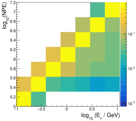
Figure 6 shows the likelihood matrix for both and events, evaluated according to the binning described in Section 4.3 and including the contribution of the background.
4.5 Uncertainties
The total uncertainty on the atmospheric neutrino spectrum reconstruction is evaluated in each energy bin, including both contributions from statistics and systematic effects.
Statistics
The statistical uncertainty is due to the stochastic fluctuations that occur in the data bins. The amount of this fluctuations is visible in Figure 5, for each observable bin. In order to evaluate their impact in the final unfolded spectrum, 1000 toy data sets have been generated, each time varying the bin content according to a Poisson distribution. The final distribution in each bin of the unfolded spectrum is then fit with a Gaussian function, whose is quoted as the statistical uncertainty. The statistical contribution ranges from 5% in the bins with highest statistics up to 15% in the highest-energy bins.
Selection criteria
The selection procedure is in general not intended to produce any bias on the final sample. As explained in Section 4.1, fiducial cuts have been used in the unfolding procedure in order to improve the accuracy of the probability evaluations. The energy range of the final reconstructed spectrum is well contained inside the energy range of the Monte Carlo generated events, guaranteeing that the fiducial cuts do not introduce any bias. The neutrino flavor identification based on the time residual selection, on the other hand, could bring some uncertainty in the data bins where the statistics is low: an even small variation in the chosen cut value of could result in a substantially different value of the unfolded flux, due to the wide stochastic fluctuations. The whole analysis has been therefore performed by varying the nominal cut value of by 1 ns steps in a [ -5 ns, +5 ns ] time window. The differences in the unfolded flux are relevant in the bins with less statistics, for the reasons explained above. The total contribution to the bin uncertainty is evaluated as the standard deviation of the flux values distribution in each bin.
Flavor oscillation
The current uncertainties on the global fit oscillation parameters are reported in Table 2, which are assumed to be Gaussian. A toy MC has been used to generate 1000 data sets, randomly varying the oscillation parameters within the experimental uncertainties, including the mass ordering and assuming no correlation. The final distribution in the unfolded flux is fit in each bin with a Gaussian function. Since the resulting dispersion is rather small in every bin, the total per-bin uncertainty contribution is quoted as the displacement of the distribution fit peak with respect to the nominal flux value. The total contribution from oscillation parameters uncertainty is estimated to be below 1% on the entire spectrum. The only exception is the first bin of the spectrum, where oscillation effects are not negligible, which results into an uncertainty corresponding to a of 1.2%.
| Parameter | NH | IH |
Cross–section
The uncertainties on neutrino cross-section impact directly on the number of observed events. In the MC simulation process, as described in Section 3, neutrino interactions are managed by the GENIE software. The full list of uncertainty sources considered by GENIE is provided in [41]. A comprehensive handling of the whole list is not trivial, since it requires the simultaneous calculation of modified interaction probabilities in a wide parameter space. In this study, the evaluation of the cross-section uncertainty is based on experimental measurements provided by the T2K Collaboration [47, 48, 49], extrapolated from the associated data releases. Assuming the uncertainty on the measured cross section values to be Gaussian, the related visible spectrum is modified accordingly, within 1 interval. The propagated uncertainty on the unfolded flux is evaluated by unfolding 1000 toy MC data sets, with NPE bin contents altered according to random variations of the cross section parameters. The unfolded spectra distributions are then fit in each bin with a Gaussian function, whose is quoted as the related uncertainty contribution. The uncertainty in the neutrino cross-section values has a large impact in the final reconstructed flux, up to 20%.
Unfolding procedure
Although the iterative Bayesian unfolding method is data-driven, the particular MC sample may have an influence on the final result. This means that the initial estimation of the likelihood matrix may have an intrinsic bias, as well as the choice of the prior. The relative impact should be small, but it can have an impact in the unfolding bins with low statistics. The net effect cannot be exactly computed, but a reliable estimation can be achieved by unfolding modified data sets, generated by assuming a primary MC distribution reasonably far from the one used to evaluate the probabilities.
The modified spectra are produced from the original MC by means of a re-weighting procedure. The new spectrum can be expressed in the -th unfolding bin as:
| (6) |
where acts on the absolute normalization and on the shape of the primary spectrum. These two parameters are considered to range in the following intervals: 0.05 for and 0.2 for .
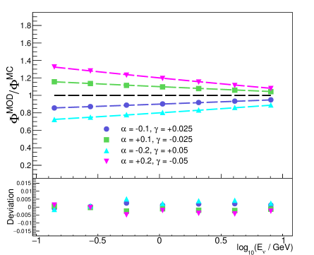
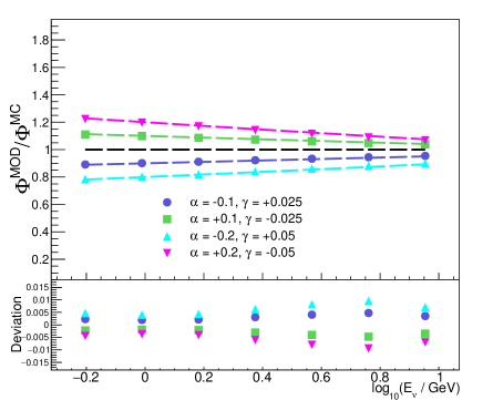
The size of variation corresponds approximately to a 1 uncertainty interval in the predicted spectra. In Figure 7 the comparison between each toy data sample and the corresponding unfolding result is reported, together with the fractional deviation between the input and the unfolded result. The deviation is below 1% and turns out to be slightly higher in the case of maximum variation of and in the bins with lower statistics. The conditional probabilities used in the unfolding procedure have been carefully evaluated by using different methods for both and samples. The relative deviations obtained for different energy bins and different NPE bins are reported in Table 3, as an example, for the sample. The effect on the obtained spectra turns out to be negligible.
| -1 – -0.5 | -0.5 – 0.36 | 0.36 – 1.1 | |
| 5 – 5.5 | 0.030 | 0.055 | 0.040 |
| 5.5 – 6.3 | – | 0.005 | 0.075 |
| 6.3 – 7.2 | – | – | 0.005 |
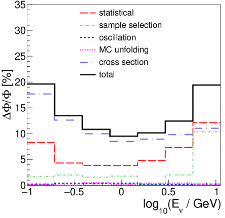
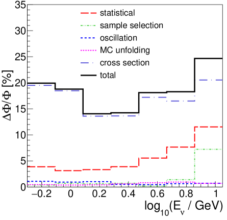
The contributions of each uncertainty source are reported in Figure 8, for each unfolding bin. The total uncertainty reported is calculated as the sum in quadrature of all contributions. The neutrino cross-section uncertainty represents the dominant contribution over the whole unfolded spectrum. The statistical uncertainty has also an important weight in high-energy bins. The total flux uncertainty ranges from a minimum value of 10-15% in the (1 GeV) energy region, up to a 20-25% in the edge bins.
5 Results and discussion
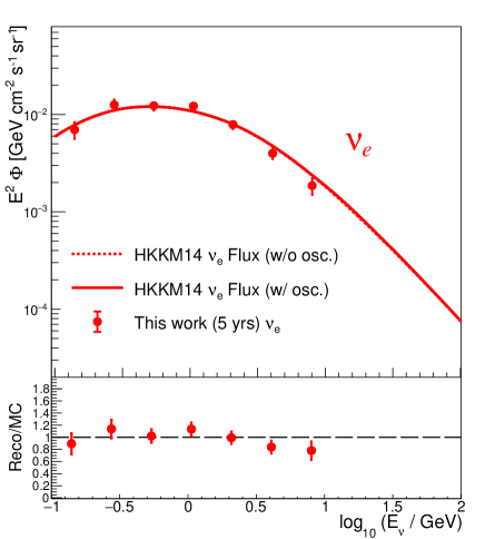
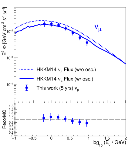
The unfolded and energy spectra are shown In Figure 9. The binning is described in Section 4.4. The predicted HKKM14 flux [33] is also reported, both at the source and including oscillation effects along the baseline. The oscillation-induced flux deficit in the flux below 10 GeV is clearly visible.
JUNO is able to reconstruct the energy spectrum of atmospheric neutrinos in the energy range [100 MeV - 10 GeV], usually referred to as the low-energy” region. This work, although based on simulated data only, shows the good capabilities of a large LS based detector like JUNO to measure the atmospheric neutrino flux. The energy region considered is already populated by other measurements, however some discrepancies still remain. JUNO can provide additional information about this interesting energy region, helping models in constraining their predictions. The quoted uncertainty is competitive with present experimental results and shows a margin of improvement by the increase of exposure time. Although JUNO’s design is not optimized for atmospheric neutrino physics, the extremely good performances in the atmospheric neutrino energy reconstruction can be fully exploited for the measurement of the energy spectrum. Moreover, atmospheric neutrinos are a natural source which will be fully accessible from the beginning of data taking.
6 Conclusions
The JUNO detector has been designed from the beginning as a state-of-the-art detector for neutrino physics. The large dimensions of the detector, as well as its dense instrumentation, pave the way to an entire series of measurements, in a multi-purpose approach. The atmospheric neutrino flux is a natural source that can be observed, from the very beginning of data-taking. Although the detector design is not optimized for this class of events, the large active volume and the fine energy resolution allow to reconstruct the energy spectrum with a competitive precision, especially in the low-energy region.
In this work, a large set of MC events has been generated to evaluate the detector performances. A smaller set has been used to simulate the real data. Thanks to the timing performances of JUNO, the flavor of primary neutrinos can be separated with a limited residual contamination. A rejection power of the order of has been applied to reduce atmospheric muon background. The atmospheric neutrino energy spectrum has been reconstructed in the energy range [100 MeV - 10 GeV], separately for and , assuming a 5 years detector livetime. The reconstructed spectra lie inside an interesting energy region, where previous measurements show some discrepancies. The results obtained show the good performance of JUNO in detecting the atmospheric neutrino flux in the low energy region, where theoretical models have large uncertainties. The inferred information can provide a fruitful input to constrain flux predictions, which are essential to evaluate the impact of atmospheric neutrinos in the search of rare events.
Acknowledgements
We are grateful for the ongoing cooperation from the China General Nuclear Power Group. This work was supported by the Chinese Academy of Sciences, the National Key R&D Program of China, the CAS Center for Excellence in Particle Physics, Wuyi University, and the Tsung-Dao Lee Institute of Shanghai Jiao Tong University in China, the Institut National de Physique Nucléaire et de Physique de Particules (IN2P3) in France, the Istituto Nazionale di Fisica Nucleare (INFN) in Italy, the Italian-Chinese collaborative research program MAECI-NSFC, the Fond de la Recherche Scientifique (F.R.S-FNRS) and FWO under the “Excellence of Science - EOS in Belgium, the Conselho Nacional de Desenvolvimento Científico e Tecnològico in Brazil, the Agencia Nacional de Investigacion y Desarrollo in Chile, the Charles University Research Centre and the Ministry of Education, Youth, and Sports in Czech Republic, the Deutsche Forschungsgemeinschaft (DFG), the Helmholtz Association, and the Cluster of Excellence PRISMA+ in Germany, the Joint Institute of Nuclear Research (JINR) and Lomonosov Moscow State University in Russia, the joint Russian Science Foundation (RSF) and National Natural Science Foundation of China (NSFC) research program, the MOST and MOE in Taiwan, the Chulalongkorn University and Suranaree University of Technology in Thailand, and the University of California at Irvine in USA.
References
-
[1]
G. D. Barr, T. K. Gaisser, P. Lipari, S. Robbins, T. Stanev,
Three-dimensional
calculation of atmospheric neutrinos, Phys. Rev. D 70 (2004) 023006.
doi:10.1103/PhysRevD.70.023006.
URL https://link.aps.org/doi/10.1103/PhysRevD.70.023006 -
[2]
M. Honda, T. Kajita, K. Kasahara, S. Midorikawa, T. Sanuki,
Calculation of
atmospheric neutrino flux using the interaction model calibrated with
atmospheric muon data, Phys. Rev. D 75 (2007) 043006.
doi:10.1103/PhysRevD.75.043006.
URL https://link.aps.org/doi/10.1103/PhysRevD.75.043006 -
[3]
T. K. Gaisser, M. Honda,
Flux of
Atmospheric Neutrinos, Annual Review of Nuclear and Particle Science
52 (1) (2002) 153–199.
arXiv:https://doi.org/10.1146/annurev.nucl.52.050102.090645, doi:10.1146/annurev.nucl.52.050102.090645.
URL https://doi.org/10.1146/annurev.nucl.52.050102.090645 - [4] M. Guan, et al., A parametrization of the cosmic-ray muon flux at sea-level (2015). arXiv:1509.06176.
- [5] T. K. Gaisser, Cosmic Rays and Particle Physics, 1991.
- [6] J. R. Hoerandel, Models of the knee in the energy spectrum of cosmic rays, Astropart. Phys. 21 (2004) 241–265. arXiv:astro-ph/0402356, doi:10.1016/j.astropartphys.2004.01.004.
-
[7]
E. Richard, et al.,
Measurements of
the atmospheric neutrino flux by Super-Kamiokande: Energy spectra,
geomagnetic effects, and solar modulation, Phys. Rev. D 94 (2016) 052001.
doi:10.1103/PhysRevD.94.052001.
URL https://link.aps.org/doi/10.1103/PhysRevD.94.052001 -
[8]
M. G. Aartsen, et al.,
Measurement of
the atmospheric flux in IceCube, Phys. Rev. Lett. 110 (2013)
151105.
doi:10.1103/PhysRevLett.110.151105.
URL https://link.aps.org/doi/10.1103/PhysRevLett.110.151105 -
[9]
M. G. Aartsen, et al.,
Measurement of the
atmospheric Spectrum with IceCube, Phys. Rev. D 91 (2015) 122004.
doi:10.1103/PhysRevD.91.122004.
URL https://link.aps.org/doi/10.1103/PhysRevD.91.122004 -
[10]
R. Abbasi, et al.,
Measurement of the
atmospheric neutrino energy spectrum from 100 GeV to 400 TeV with
IceCube, Phys. Rev. D 83 (2011) 012001.
doi:10.1103/PhysRevD.83.012001.
URL https://link.aps.org/doi/10.1103/PhysRevD.83.012001 -
[11]
K. Daum, et al., Determination of the
atmospheric neutrino spectra with the Fréjus detector, Zeitschrift
für physik C Particles and Fields 66 (3) (1995) 417–428.
doi:10.1007/BF01556368.
URL https://doi.org/10.1007/BF01556368 -
[12]
R. Enberg, M. H. Reno, I. Sarcevic,
Prompt neutrino
fluxes from atmospheric charm, Phys. Rev. D 78 (2008) 043005.
doi:10.1103/PhysRevD.78.043005.
URL https://link.aps.org/doi/10.1103/PhysRevD.78.043005 - [13] M. R. A.D. Martin, A. Stasto, Prompt neutrinos from atmospheric c-cbar and b-bbar production and the gluon at very small x, Acta Phys. Polon. B 34 (2003) 3273.
-
[14]
G. Fiorentini, V. A. Naumov, F. L. Villante,
Atmospheric
neutrino flux supported by recent muon experiments, Physics Letters B
510 (1) (2001) 173 – 188.
doi:https://doi.org/10.1016/S0370-2693(01)00572-X.
URL http://www.sciencedirect.com/science/article/pii/S037026930100572X -
[15]
M. Aartsen, et al.,
Measurement of
atmospheric neutrino oscillations at 6–56 GeV with IceCube DeepCore,
Phys. Rev. Lett. 120 (2018) 071801.
doi:10.1103/PhysRevLett.120.071801.
URL https://link.aps.org/doi/10.1103/PhysRevLett.120.071801 -
[16]
C. Achar, et al.,
Detection
of muons produced by cosmic ray neutrinos deep underground, Physics Letters
18 (2) (1965) 196 – 199.
doi:https://doi.org/10.1016/0031-9163(65)90712-2.
URL http://www.sciencedirect.com/science/article/pii/0031916365907122 -
[17]
F. Reines, et al.,
Evidence for
High-Energy Cosmic-Ray Neutrino Interactions, Phys. Rev. Lett.
15 (1965) 429–433.
doi:10.1103/PhysRevLett.15.429.
URL https://link.aps.org/doi/10.1103/PhysRevLett.15.429 -
[18]
Y. Fukuda, et al.,
Evidence for
Oscillation of Atmospheric Neutrinos, Phys. Rev. Lett. 81 (1998)
1562–1567.
doi:10.1103/PhysRevLett.81.1562.
URL https://link.aps.org/doi/10.1103/PhysRevLett.81.1562 - [19] B. Abi, et al., Deep Underground Neutrino Experiment (DUNE), Far Detector Technical Design Report, Volume II: DUNE Physics (2020). arXiv:2002.03005.
- [20] H.-K. Proto-Collaboration, :, K. Abe, et al., Hyper-Kamiokande Design Report (2018). arXiv:1805.04163.
-
[21]
A. Kumar, others., Physics
potential of the ICAL detector at the India-based Neutrino
Observatory (INO), Pramana - J Phys 88 (5) (2017) 79.
doi:10.1007/s12043-017-1373-4.
URL https://doi.org/10.1007/s12043-017-1373-4 -
[22]
S. Adrián-Martínez, others.,
Letter of intent for
KM3net 2.0, Journal of Physics G: Nuclear and Particle Physics 43 (8)
(2016) 084001.
doi:10.1088/0954-3899/43/8/084001.
URL https://doi.org/10.1088/0954-3899/43/8/084001 -
[23]
M. G. Aartsen, others.,
PINGU: a vision for
neutrino and particle physics at the South Pole, Journal of Physics G:
Nuclear and Particle Physics 44 (5) (2017) 054006.
doi:10.1088/1361-6471/44/5/054006.
URL https://doi.org/10.1088/1361-6471/44/5/054006 -
[24]
M. G. Aartsen, et al.,
Measurement of the
energy spectrum with IceCube-79, The European Physical Journal C
77 (10) (2017) 692.
doi:10.1140/epjc/s10052-017-5261-3.
URL https://doi.org/10.1140/epjc/s10052-017-5261-3 -
[25]
F. An, et al.,
Neutrino physics
with JUNO, Journal of Physics G: Nuclear and Particle Physics 43 (3)
(2016) 030401.
doi:10.1088/0954-3899/43/3/030401.
URL https://doi.org/10.1088%2F0954-3899%2F43%2F3%2F030401 - [26] T. Adam, et al., JUNO Conceptual Design Report (2015). arXiv:1508.07166.
- [27] C. Cao, et al., Mass production and characterization of 3-inch PMTs for the JUNO experiment, submitted to Nucl. Instr. Meth. A. (2021). arXiv:2102.11538.
-
[28]
T. Adam, et al.,
The
OPERA experiment Target Tracker, Nuclear Instruments and Methods in
Physics Research Section A: Accelerators, Spectrometers, Detectors and
Associated Equipment 577 (3) (2007) 523 – 539.
doi:https://doi.org/10.1016/j.nima.2007.04.147.
URL http://www.sciencedirect.com/science/article/pii/S0168900207007553 -
[29]
A. Abusleme, et al.,
Optimization
of the JUNO liquid scintillator composition using a Daya Bay
antineutrino detector, Nuclear Instruments and Methods in Physics Research
Section A: Accelerators, Spectrometers, Detectors and Associated Equipment
(2020) 164823doi:10.1016/j.nima.2020.164823.
URL http://www.sciencedirect.com/science/article/pii/S0168900220312201 -
[30]
P. Lombardi, et al.,
Distillation
and stripping pilot plants for the JUNO neutrino detector: Design,
operations and reliability, Nuclear Instruments and Methods in Physics
Research Section A: Accelerators, Spectrometers, Detectors and Associated
Equipment 925 (2019) 6 – 17.
doi:https://doi.org/10.1016/j.nima.2019.01.071.
URL http://www.sciencedirect.com/science/article/pii/S0168900219301299 - [31] A. Abusleme, et al., Calibration strategy of the JUNO Experiment, accepted for publication by JHEP (2020). arXiv:2011.06405.
-
[32]
J. A. Formaggio, G. P. Zeller,
From ev to EefV:
Neutrino cross sections across energy scales, Rev. Mod. Phys. 84 (2012)
1307–1341.
doi:10.1103/RevModPhys.84.1307.
URL https://link.aps.org/doi/10.1103/RevModPhys.84.1307 -
[33]
M. Honda, M. S. Athar, T. Kajita, K. Kasahara, S. Midorikawa,
Atmospheric
neutrino flux calculation using the NRLMSISE-00 atmospheric model, Phys.
Rev. D 92 (2015) 023004.
doi:10.1103/PhysRevD.92.023004.
URL https://link.aps.org/doi/10.1103/PhysRevD.92.023004 -
[34]
T. Sanuki, et al., Precise measurement
of cosmic-ray proton and helium spectra with the BESS spectrometer, The
Astrophysical Journal 545 (2) (2000) 1135–1142.
doi:10.1086/317873.
URL https://doi.org/10.1086%2F317873 - [35] S. Haino, et al., Measurements of primary and atmospheric cosmic-ray spectra with the BESS-TeV spectrometer, Physics Letters B 594 (1) (2004) 35 – 46. doi:https://doi.org/10.1016/j.physletb.2004.05.019.
- [36] J. Alcaraz, et al., Protons in near Earth orbit, Physics Letters B 472 (1) (2000) 215 – 226. doi:https://doi.org/10.1016/S0370-2693(99)01427-6.
- [37] S. Roesler, R. Engel, J. Ranft, The Monte Carlo Event Generator DPMJET-III, Advanced Monte Carlo for Radiation Physics, Particle Transport Simulation and Applications (2001) 1033–1038doi:10.1007/978-3-642-18211-2_166.
-
[38]
K. Niita, T. Sato, H. Iwase, H. Nose, H. Nakashima, L. Sihver,
Phits—a
particle and heavy ion transport code system, Radiation Measurements 41 (9)
(2006) 1080–1090, space Radiation Transport, Shielding, and Risk Assessment
Models.
doi:https://doi.org/10.1016/j.radmeas.2006.07.013.
URL https://www.sciencedirect.com/science/article/pii/S1350448706001351 -
[39]
M. Tanabashi, et al.,
Review of
Particle Physics, Phys. Rev. D 98 (2018) 030001.
doi:10.1103/PhysRevD.98.030001.
URL https://link.aps.org/doi/10.1103/PhysRevD.98.030001 -
[40]
C. Andreopoulos, et al.,
The
GENIE neutrino Monte Carlo generator, Nuclear Instruments and Methods in
Physics Research Section A: Accelerators, Spectrometers, Detectors and
Associated Equipment 614 (1) (2010) 87 – 104.
doi:https://doi.org/10.1016/j.nima.2009.12.009.
URL http://www.sciencedirect.com/science/article/pii/S0168900209023043 - [41] C. Andreopoulos, et al., The GENIE Neutrino Monte Carlo Generator: Physics and User Manual, 2015. arXiv:1510.05494.
-
[42]
J. H. Zou, et al.,
SNiPER: an
offline software framework for non-collider physics experiments, Journal of
Physics: Conference Series 664 (7) (2015) 072053.
doi:10.1088/1742-6596/664/7/072053.
URL https://doi.org/10.1088%2F1742-6596%2F664%2F7%2F072053 - [43] M. Guan, et al., A parametrization of the cosmic-ray muon flux at sea-level (2015). arXiv:1509.06176.
-
[44]
V. Kudryavtsev,
Muon
simulation codes MUSIC and MUSUN for underground physics, Computer
Physics Communications 180 (3) (2009) 339 – 346.
doi:https://doi.org/10.1016/j.cpc.2008.10.013.
URL http://www.sciencedirect.com/science/article/pii/S0010465508003640 -
[45]
G. Settanta, et al.,
e- discrimination at
high energy in the JUNO detector, EPJ Web Conf. 209 (2019) 01011.
doi:10.1051/epjconf/201920901011.
URL https://doi.org/10.1051/epjconf/201920901011 -
[46]
G. D’Agostini,
A
multidimensional unfolding method based on Bayes’ theorem, Nuclear
Instruments and Methods in Physics Research Section A: Accelerators,
Spectrometers, Detectors and Associated Equipment 362 (2) (1995) 487 – 498.
doi:https://doi.org/10.1016/0168-9002(95)00274-X.
URL http://www.sciencedirect.com/science/article/pii/016890029500274X -
[47]
K. Abe, et al.,
Measurement
of the Inclusive Electron Neutrino Charged Current Cross Section on Carbon
with the T2K Near Detector, Phys. Rev. Lett. 113 (2014) 241803.
doi:10.1103/PhysRevLett.113.241803.
URL https://link.aps.org/doi/10.1103/PhysRevLett.113.241803 -
[48]
K. Abe, et al.,
Measurement of the
charged-current quasielastic cross
section on carbon with the ND280 detector at T2K, Phys. Rev. D 92 (2015)
112003.
doi:10.1103/PhysRevD.92.112003.
URL https://link.aps.org/doi/10.1103/PhysRevD.92.112003 -
[49]
K. Abe, et al.,
First measurement
of the muon neutrino charged current single pion production cross section on
water with the T2K near detector, Phys. Rev. D 95 (2017) 012010.
doi:10.1103/PhysRevD.95.012010.
URL https://link.aps.org/doi/10.1103/PhysRevD.95.012010
The JUNO Collaboration
Angel Abusleme5,
Thomas Adam45,
Shakeel Ahmad66,
Rizwan Ahmed66,
Sebastiano Aiello55,
Muhammad Akram66,
Fengpeng An29,
Guangpeng An10,
Qi An22,
Giuseppe Andronico55,
Nikolay Anfimov67,
Vito Antonelli57,
Tatiana Antoshkina67,
Burin Asavapibhop71,
João Pedro Athayde Marcondes de André45,
Didier Auguste43,
Andrej Babic70,
Wander Baldini56,
Andrea Barresi58,
Eric Baussan45,
Marco Bellato60,
Antonio Bergnoli60,
Enrico Bernieri64,
Thilo Birkenfeld48,
Sylvie Blin43,
David Blum54,
Simon Blyth40,
Anastasia Bolshakova67,
Mathieu Bongrand47,
Clément Bordereau44,40,
Dominique Breton43,
Augusto Brigatti57,
Riccardo Brugnera61,
Riccardo Bruno55,
Antonio Budano64,
Mario Buscemi55,
Jose Busto46,
Ilya Butorov67,
Anatael Cabrera43,
Hao Cai34,
Xiao Cai10,
Yanke Cai10,
Zhiyan Cai10,
Antonio Cammi59,
Agustin Campeny5,
Chuanya Cao10,
Guofu Cao10,
Jun Cao10,
Rossella Caruso55,
Cédric Cerna44,
Jinfan Chang10,
Yun Chang39,
Pingping Chen18,
Po-An Chen40,
Shaomin Chen13,
Xurong Chen26,
Yi-Wen Chen38,
Yixue Chen11,
Yu Chen20,
Zhang Chen10,
Jie Cheng10,
Yaping Cheng7,
Alexey Chetverikov67,
Davide Chiesa58,
Pietro Chimenti3,
Artem Chukanov67,
Gérard Claverie44,
Catia Clementi62,
Barbara Clerbaux2,
Selma Conforti Di Lorenzo43,
Daniele Corti60,
Salvatore Costa55,
Flavio Dal Corso60,
Olivia Dalager74,
Christophe De La Taille43,
Jiawei Deng34,
Zhi Deng13,
Ziyan Deng10,
Wilfried Depnering52,
Marco Diaz5,
Xuefeng Ding57,
Yayun Ding10,
Bayu Dirgantara73,
Sergey Dmitrievsky67,
Tadeas Dohnal41,
Dmitry Dolzhikov67,
Georgy Donchenko69,
Jianmeng Dong13,
Evgeny Doroshkevich68,
Marcos Dracos45,
Frédéric Druillole44,
Shuxian Du37,
Stefano Dusini60,
Martin Dvorak41,
Timo Enqvist42,
Heike Enzmann52,
Andrea Fabbri64,
Lukas Fajt70,
Donghua Fan24,
Lei Fan10,
Can Fang28,
Jian Fang10,
Wenxing Fang10,
Marco Fargetta55,
Dmitry Fedoseev67,
Vladko Fekete70,
Li-Cheng Feng38,
Qichun Feng21,
Richard Ford57,
Andrey Formozov57,
Amélie Fournier44,
Haonan Gan32,
Feng Gao48,
Alberto Garfagnini61,
Christoph Genster50,
Marco Giammarchi57,
Agnese Giaz61,
Nunzio Giudice55,
Maxim Gonchar67,
Guanghua Gong13,
Hui Gong13,
Oleg Gorchakov67,
Yuri Gornushkin67,
Alexandre Göttel50,48,
Marco Grassi61,
Christian Grewing51,
Vasily Gromov67,
Minghao Gu10,
Xiaofei Gu37,
Yu Gu19,
Mengyun Guan10,
Nunzio Guardone55,
Maria Gul66,
Cong Guo10,
Jingyuan Guo20,
Wanlei Guo10,
Xinheng Guo8,
Yuhang Guo35,50,
Paul Hackspacher52,
Caren Hagner49,
Ran Han7,
Yang Han43,
Muhammad Sohaib Hassan66,
Miao He10,
Wei He10,
Tobias Heinz54,
Patrick Hellmuth44,
Yuekun Heng10,
Rafael Herrera5,
Daojin Hong28,
YuenKeung Hor20,
Shaojing Hou10,
Yee Hsiung40,
Bei-Zhen Hu40,
Hang Hu20,
Jianrun Hu10,
Jun Hu10,
Shouyang Hu9,
Tao Hu10,
Zhuojun Hu20,
Chunhao Huang20,
Guihong Huang10,
Hanxiong Huang9,
Qinhua Huang45,
Wenhao Huang25,
Xin Huang10,
Xingtao Huang25,
Yongbo Huang28,
Jiaqi Hui30,
Lei Huo21,
Wenju Huo22,
Cédric Huss44,
Safeer Hussain66,
Antonio Insolia55,
Ara Ioannisian1,
Roberto Isocrate60,
Beatrice Jelmini61,
Kuo-Lun Jen38,
Ignacio Jeria5,
Xiaolu Ji10,
Xingzhao Ji20,
Huihui Jia33,
Junji Jia34,
Siyu Jian9,
Di Jiang22,
Xiaoshan Jiang10,
Ruyi Jin10,
Xiaoping Jing10,
Cécile Jollet44,
Jari Joutsenvaara42,
Sirichok Jungthawan73,
Leonidas Kalousis45,
Philipp Kampmann50,
Li Kang18,
Michael Karagounis51,
Narine Kazarian1,
Waseem Khan35,
Khanchai Khosonthongkee73,
Denis Korablev67,
Konstantin Kouzakov69,
Alexey Krasnoperov67,
Zinovy Krumshteyn67,
Andre Kruth51,
Nikolay Kutovskiy67,
Pasi Kuusiniemi42,
Tobias Lachenmaier54,
Cecilia Landini57,
Sébastien Leblanc44,
Victor Lebrin47,
Frederic Lefevre47,
Ruiting Lei18,
Rupert Leitner41,
Jason Leung38,
Demin Li37,
Fei Li10,
Fule Li13,
Haitao Li20,
Huiling Li10,
Jiaqi Li20,
Mengzhao Li10,
Min Li11,
Nan Li10,
Nan Li16,
Qingjiang Li16,
Ruhui Li10,
Shanfeng Li18,
Tao Li20,
Weidong Li10,14,
Weiguo Li10,
Xiaomei Li9,
Xiaonan Li10,
Xinglong Li9,
Yi Li18,
Yufeng Li10,
Zhaohan Li10,
Zhibing Li20,
Ziyuan Li20,
Hao Liang9,
Hao Liang22,
Jingjing Liang28,
Daniel Liebau51,
Ayut Limphirat73,
Sukit Limpijumnong73,
Guey-Lin Lin38,
Shengxin Lin18,
Tao Lin10,
Jiajie Ling20,
Ivano Lippi60,
Fang Liu11,
Haidong Liu37,
Hongbang Liu28,
Hongjuan Liu23,
Hongtao Liu20,
Hui Liu19,
Jianglai Liu30,31,
Jinchang Liu10,
Min Liu23,
Qian Liu14,
Qin Liu22,
Runxuan Liu50,48,
Shuangyu Liu10,
Shubin Liu22,
Shulin Liu10,
Xiaowei Liu20,
Xiwen Liu28,
Yan Liu10,
Yunzhe Liu10,
Alexey Lokhov69,68,
Paolo Lombardi57,
Claudio Lombardo55,
Kai Loo52,
Chuan Lu32,
Haoqi Lu10,
Jingbin Lu15,
Junguang Lu10,
Shuxiang Lu37,
Xiaoxu Lu10,
Bayarto Lubsandorzhiev68,
Sultim Lubsandorzhiev68,
Livia Ludhova50,48,
Fengjiao Luo10,
Guang Luo20,
Pengwei Luo20,
Shu Luo36,
Wuming Luo10,
Vladimir Lyashuk68,
Bangzheng Ma25,
Qiumei Ma10,
Si Ma10,
Xiaoyan Ma10,
Xubo Ma11,
Jihane Maalmi43,
Yury Malyshkin67,
Fabio Mantovani56,
Francesco Manzali61,
Xin Mao7,
Yajun Mao12,
Stefano M. Mari64,
Filippo Marini61,
Sadia Marium66,
Cristina Martellini64,
Gisele Martin-Chassard43,
Agnese Martini63,
Davit Mayilyan1,
Ints Mednieks65,
Yue Meng30,
Anselmo Meregaglia44,
Emanuela Meroni57,
David Meyhöfer49,
Mauro Mezzetto60,
Jonathan Miller6,
Lino Miramonti57,
Salvatore Monforte55,
Paolo Montini64,
Michele Montuschi56,
Axel Müller54,
Pavithra Muralidharan51,
Massimiliano Nastasi58,
Dmitry V. Naumov67,
Elena Naumova67,
Diana Navas-Nicolas43,
Igor Nemchenok67,
Minh Thuan Nguyen Thi38,
Feipeng Ning10,
Zhe Ning10,
Hiroshi Nunokawa4,
Lothar Oberauer53,
Juan Pedro Ochoa-Ricoux74,5,
Alexander Olshevskiy67,
Domizia Orestano64,
Fausto Ortica62,
Rainer Othegraven52,
Hsiao-Ru Pan40,
Alessandro Paoloni63,
Nina Parkalian51,
Sergio Parmeggiano57,
Yatian Pei10,
Nicomede Pelliccia62,
Anguo Peng23,
Haiping Peng22,
Frédéric Perrot44,
Pierre-Alexandre Petitjean2,
Fabrizio Petrucci64,
Oliver Pilarczyk52,
Luis Felipe Piñeres Rico45,
Artyom Popov69,
Pascal Poussot45,
Wathan Pratumwan73,
Ezio Previtali58,
Fazhi Qi10,
Ming Qi27,
Sen Qian10,
Xiaohui Qian10,
Zhen Qian20,
Hao Qiao12,
Zhonghua Qin10,
Shoukang Qiu23,
Muhammad Usman Rajput66,
Gioacchino Ranucci57,
Neill Raper20,
Alessandra Re57,
Henning Rebber49,
Abdel Rebii44,
Bin Ren18,
Jie Ren9,
Taras Rezinko67,
Barbara Ricci56,
Markus Robens51,
Mathieu Roche44,
Narongkiat Rodphai71,
Aldo Romani62,
Bedřich Roskovec74,
Christian Roth51,
Xiangdong Ruan28,
Xichao Ruan9,
Saroj Rujirawat73,
Arseniy Rybnikov67,
Andrey Sadovsky67,
Paolo Saggese57,
Giuseppe Salamanna64,
Simone Sanfilippo64,
Anut Sangka72,
Nuanwan Sanguansak73,
Utane Sawangwit72,
Julia Sawatzki53,
Fatma Sawy61,
Michaela Schever50,48,
Jacky Schuler45,
Cédric Schwab45,
Konstantin Schweizer53,
Alexandr Selyunin67,
Andrea Serafini56,
Giulio Settanta50,64,
Mariangela Settimo47,
Zhuang Shao35,
Vladislav Sharov67,
Arina Shaydurova67,
Jingyan Shi10,
Yanan Shi10,
Vitaly Shutov67,
Andrey Sidorenkov68,
Fedor Šimkovic70,
Chiara Sirignano61,
Jaruchit Siripak73,
Monica Sisti58,
Maciej Slupecki42,
Mikhail Smirnov20,
Oleg Smirnov67,
Thiago Sogo-Bezerra47,
Sergey Sokolov67,
Julanan Songwadhana73,
Boonrucksar Soonthornthum72,
Albert Sotnikov67,
Ondřej Šrámek41,
Warintorn Sreethawong73,
Achim Stahl48,
Luca Stanco60,
Konstantin Stankevich69,
Dušan Štefánik70,
Hans Steiger52,53,
Jochen Steinmann48,
Tobias Sterr54,
Matthias Raphael Stock53,
Virginia Strati56,
Alexander Studenikin69,
Gongxing Sun10,
Shifeng Sun11,
Xilei Sun10,
Yongjie Sun22,
Yongzhao Sun10,
Narumon Suwonjandee71,
Michal Szelezniak45,
Jian Tang20,
Qiang Tang20,
Quan Tang23,
Xiao Tang10,
Alexander Tietzsch54,
Igor Tkachev68,
Tomas Tmej41,
Konstantin Treskov67,
Andrea Triossi45,
Giancarlo Troni5,
Wladyslaw Trzaska42,
Cristina Tuve55,
Nikita Ushakov68,
Johannes van den Boom51,
Stefan van Waasen51,
Guillaume Vanroyen47,
Nikolaos Vassilopoulos10,
Vadim Vedin65,
Giuseppe Verde55,
Maxim Vialkov69,
Benoit Viaud47,
Moritz Vollbrecht50,48,
Cristina Volpe43,
Vit Vorobel41,
Dmitriy Voronin68,
Lucia Votano63,
Pablo Walker5,
Caishen Wang18,
Chung-Hsiang Wang39,
En Wang37,
Guoli Wang21,
Jian Wang22,
Jun Wang20,
Kunyu Wang10,
Lu Wang10,
Meifen Wang10,
Meng Wang23,
Meng Wang25,
Ruiguang Wang10,
Siguang Wang12,
Wei Wang27,
Wei Wang20,
Wenshuai Wang10,
Xi Wang16,
Xiangyue Wang20,
Yangfu Wang10,
Yaoguang Wang10,
Yi Wang13,
Yi Wang24,
Yifang Wang10,
Yuanqing Wang13,
Yuman Wang27,
Zhe Wang13,
Zheng Wang10,
Zhimin Wang10,
Zongyi Wang13,
Muhammad Waqas66,
Apimook Watcharangkool72,
Lianghong Wei10,
Wei Wei10,
Wenlu Wei10,
Yadong Wei18,
Liangjian Wen10,
Christopher Wiebusch48,
Steven Chan-Fai Wong20,
Bjoern Wonsak49,
Diru Wu10,
Fangliang Wu27,
Qun Wu25,
Wenjie Wu34,
Zhi Wu10,
Michael Wurm52,
Jacques Wurtz45,
Christian Wysotzki48,
Yufei Xi32,
Dongmei Xia17,
Yuguang Xie10,
Zhangquan Xie10,
Zhizhong Xing10,
Benda Xu13,
Cheng Xu23,
Donglian Xu31,30,
Fanrong Xu19,
Hangkun Xu10,
Jilei Xu10,
Jing Xu8,
Meihang Xu10,
Yin Xu33,
Yu Xu50,48,
Baojun Yan10,
Taylor Yan73,
Wenqi Yan10,
Xiongbo Yan10,
Yupeng Yan73,
Anbo Yang10,
Changgen Yang10,
Huan Yang10,
Jie Yang37,
Lei Yang18,
Xiaoyu Yang10,
Yifan Yang10,
Yifan Yang2,
Haifeng Yao10,
Zafar Yasin66,
Jiaxuan Ye10,
Mei Ye10,
Ziping Ye31,
Ugur Yegin51,
Frédéric Yermia47,
Peihuai Yi10,
Na Yin25,
Xiangwei Yin10,
Zhengyun You20,
Boxiang Yu10,
Chiye Yu18,
Chunxu Yu33,
Hongzhao Yu20,
Miao Yu34,
Xianghui Yu33,
Zeyuan Yu10,
Zezhong Yu10,
Chengzhuo Yuan10,
Ying Yuan12,
Zhenxiong Yuan13,
Ziyi Yuan34,
Baobiao Yue20,
Noman Zafar66,
Andre Zambanini51,
Vitalii Zavadskyi67,
Shan Zeng10,
Tingxuan Zeng10,
Yuda Zeng20,
Liang Zhan10,
Aiqiang Zhang13,
Feiyang Zhang30,
Guoqing Zhang10,
Haiqiong Zhang10,
Honghao Zhang20,
Jiawen Zhang10,
Jie Zhang10,
Jingbo Zhang21,
Jinnan Zhang10,
Peng Zhang10,
Qingmin Zhang35,
Shiqi Zhang20,
Shu Zhang20,
Tao Zhang30,
Xiaomei Zhang10,
Xuantong Zhang10,
Xueyao Zhang25,
Yan Zhang10,
Yinhong Zhang10,
Yiyu Zhang10,
Yongpeng Zhang10,
Yuanyuan Zhang30,
Yumei Zhang20,
Zhenyu Zhang34,
Zhijian Zhang18,
Fengyi Zhao26,
Jie Zhao10,
Rong Zhao20,
Shujun Zhao37,
Tianchi Zhao10,
Dongqin Zheng19,
Hua Zheng18,
Minshan Zheng9,
Yangheng Zheng14,
Weirong Zhong19,
Jing Zhou9,
Li Zhou10,
Nan Zhou22,
Shun Zhou10,
Tong Zhou10,
Xiang Zhou34,
Jiang Zhu20,
Kejun Zhu10,
Zhihang Zhu10,
Bo Zhuang10,
Honglin Zhuang10,
Liang Zong13,
Jiaheng Zou10.
1Yerevan Physics Institute, Yerevan, Armenia
2Université Libre de Bruxelles, Brussels, Belgium
3Universidade Estadual de Londrina, Londrina, Brazil
4Pontificia Universidade Catolica do Rio de Janeiro, Rio, Brazil
5Pontificia Universidad Católica de Chile, Santiago, Chile
6Universidad Tecnica Federico Santa Maria, Valparaiso, Chile
7Beijing Institute of Spacecraft Environment Engineering, Beijing, China
8Beijing Normal University, Beijing, China
9China Institute of Atomic Energy, Beijing, China
10Institute of High Energy Physics, Beijing, China
11North China Electric Power University, Beijing, China
12School of Physics, Peking University, Beijing, China
13Tsinghua University, Beijing, China
14University of Chinese Academy of Sciences, Beijing, China
15Jilin University, Changchun, China
16College of Electronic Science and Engineering, National University of Defense Technology, Changsha, China
17Chongqing University, Chongqing, China
18Dongguan University of Technology, Dongguan, China
19Jinan University, Guangzhou, China
20Sun Yat-Sen University, Guangzhou, China
21Harbin Institute of Technology, Harbin, China
22University of Science and Technology of China, Hefei, China
23The Radiochemistry and Nuclear Chemistry Group in University of South China, Hengyang, China
24Wuyi University, Jiangmen, China
25Shandong University, Jinan, China, and Key Laboratory of Particle Physics and Particle Irradiation of Ministry of Education, Shandong University, Qingdao, China
26Institute of Modern Physics, Chinese Academy of Sciences, Lanzhou, China
27Nanjing University, Nanjing, China
28Guangxi University, Nanning, China
29East China University of Science and Technology, Shanghai, China
30School of Physics and Astronomy, Shanghai Jiao Tong University, Shanghai, China
31Tsung-Dao Lee Institute, Shanghai Jiao Tong University, Shanghai, China
32Institute of Hydrogeology and Environmental Geology, Chinese Academy of Geological Sciences, Shijiazhuang, China
33Nankai University, Tianjin, China
34Wuhan University, Wuhan, China
35Xi’an Jiaotong University, Xi’an, China
36Xiamen University, Xiamen, China
37School of Physics and Microelectronics, Zhengzhou University, Zhengzhou, China
38Institute of Physics, National Yang Ming Chiao Tung University, Hsinchu
39National United University, Miao-Li
40Department of Physics, National Taiwan University, Taipei
41Charles University, Faculty of Mathematics and Physics, Prague, Czech Republic
42University of Jyvaskyla, Department of Physics, Jyvaskyla, Finland
43IJCLab, Université Paris-Saclay, CNRS/IN2P3, 91405 Orsay, France
44Univ. Bordeaux, CNRS, CENBG, UMR 5797, F-33170 Gradignan, France
45IPHC, Université de Strasbourg, CNRS/IN2P3, F-67037 Strasbourg, France
46Centre de Physique des Particules de Marseille, Marseille, France
47SUBATECH, Université de Nantes, IMT Atlantique, CNRS-IN2P3, Nantes, France
48III. Physikalisches Institut B, RWTH Aachen University, Aachen, Germany
49Institute of Experimental Physics, University of Hamburg, Hamburg, Germany
50Forschungszentrum Jülich GmbH, Nuclear Physics Institute IKP-2, Jülich, Germany
51Forschungszentrum Jülich GmbH, Central Institute of Engineering, Electronics and Analytics - Electronic Systems (ZEA-2), Jülich, Germany
52Institute of Physics, Johannes-Gutenberg Universität Mainz, Mainz, Germany
53Technische Universität München, München, Germany
54Eberhard Karls Universität Tübingen, Physikalisches Institut, Tübingen, Germany
55INFN Catania and Dipartimento di Fisica e Astronomia dell Università di Catania, Catania, Italy
56Department of Physics and Earth Science, University of Ferrara and INFN Sezione di Ferrara, Ferrara, Italy
57INFN Sezione di Milano and Dipartimento di Fisica dell Università di Milano, Milano, Italy
58INFN Milano Bicocca and University of Milano Bicocca, Milano, Italy
59INFN Milano Bicocca and Politecnico of Milano, Milano, Italy
60INFN Sezione di Padova, Padova, Italy
61Dipartimento di Fisica e Astronomia dell’Università di Padova and INFN Sezione di Padova, Padova, Italy
62INFN Sezione di Perugia and Dipartimento di Chimica, Biologia e Biotecnologie dell’Università di Perugia, Perugia, Italy
63Laboratori Nazionali di Frascati dell’INFN, Roma, Italy
64University of Roma Tre and INFN Sezione Roma Tre, Roma, Italy
65Institute of Electronics and Computer Science, Riga, Latvia
66Pakistan Institute of Nuclear Science and Technology, Islamabad, Pakistan
67Joint Institute for Nuclear Research, Dubna, Russia
68Institute for Nuclear Research of the Russian Academy of Sciences, Moscow, Russia
69Lomonosov Moscow State University, Moscow, Russia
70Comenius University Bratislava, Faculty of Mathematics, Physics and Informatics, Bratislava, Slovakia
71Department of Physics, Faculty of Science, Chulalongkorn University, Bangkok, Thailand
72National Astronomical Research Institute of Thailand, Chiang Mai, Thailand
73Suranaree University of Technology, Nakhon Ratchasima, Thailand
74Department of Physics and Astronomy, University of California, Irvine, California, USA