From one-way streets to percolation on random mixed graphs

Abstract

In most studies, street networks are considered as undirected graphs while one-way streets and their effect on shortest paths are usually ignored. Here, we first study the empirical effect of one-way streets in about $140$ cities in the world. Their presence induces a detour that persists over a wide range of distances and characterized by a non-universal exponent. The effect of one-ways on the pattern of shortest paths is then twofold: they mitigate local traffic in certain areas but create bottlenecks elsewhere. This empirical study leads naturally to consider a mixed graph model of 2d regular lattices with both undirected links and a diluted variable fraction $p$ of randomly directed links which mimics the presence of one-ways in a street network. We study the size of the strongly connected component (SCC) versus $p$ and demonstrate the existence of a threshold $p_{c}$ above which the SCC size is zero. We show numerically that this transition is non-trivial for lattices with degree less than $4$ and provide some analytical argument. We compute numerically the critical exponents for this transition and confirm previous results showing that they define a new universality class different from both the directed and standard percolation. Finally, we show that the transition on real-world graphs can be understood with random perturbations of regular lattices. The impact of one-ways on the graph properties were already the subject of a few mathematical studies, and our results show that this problem has also interesting connections with percolation, a classical model in statistical physics.

I Introduction

In most countries a majority of individuals commute by car Verbavatz:2019 and smart monitoring of traffic in cities has become crucial for enhancing productivity while reducing transport emissions Dodman:2009 ; Newman:2006 . Historically, a simple and efficient way to manage traffic is by using dedicated traffic codes, including the design of one-way streets Lay:1992 . The first official attempt to create dedicated one-way roads is said to date back to 1617 in London Homer:2006 . The ‘No Entry’ sign was officially adopted for standardization at the League of Nations convention in Geneva in 1931 Lay:1992 . To this day, one-way streets are created in order to smooth motor traffic in cities Stemley:1998 , to reduce driving time and congestion, or to preserve specific neighborhoods Venerandi:2004 from traffic.

Mathematically, street networks can be represented by graphs where the vertices are intersections and the links road segments between consecutive intersections. Almost all studies on street networks Jiang:2004 ; Buhl:2006 ; Strano:2013 ; Xie:2007 ; Lammer:2006 ; Strano:2012 ; Crucitti:2006 ; Louf:2014 ; Barthelemy:2018 ; Boeing:2019 describe street network as undirected graph but formally a network of both undirected links and one-way streets (represented by directed edges) is called a mixed graph Beck:2013 . Despite their relevance for practical applications Roberts:1978 , there are very few results available for directed street networks, except for the following one: Robbins’ theorem Robbins:1939 states that it is possible to choose a direction for each edge - called hereafter a strong orientation - of an undirected graph $G$ turning it into a directed graph that has a path from every vertex to every other vertex, if and only if $G$ is connected and has no bridge (i.e. an edge whose deletion increases the graph’s number of connected components). Robbins’ seminal result can be extended to mixed graphs Boesch:1980 , stating that if $G$ is a strongly connected mixed graph, then any undirected edge of $G$ that is not a bridge may be made directed without changing the connectivity of $G$. Hence, it is possible to turn streets into one-ways as long as their removal does not disconnect the whole street network. It is thus recursively possible for any bridgeless network to be turned into a fully directed graph. In most cities, it should then be possible to find a street-orientation that keep the network strongly connected. This theorem however does not say anything about how one-way streets modify shortest paths. In this respect, very few results were obtained: for the diameter for example, Chvatal and Thomassen Chvatal:1978 proved that if the undirected graph has a diameter $d$, then there exist a strong orientation with diameter less than the (best possible) bound $2d+2d^{2}$, but that it is also a NP-hard problem to find. It is interesting to note that for some applications, it is desirable to find a strong orientation that is not efficient, i.e. doesn’t minimize the diameter in order to discourage people from driving in certain sections Roberts:1978 .

Here, we will first discuss some empirical results about the fraction of one-way streets in cities and their effect on shortest paths. This will naturally leads us to consider the problem of percolation in mixed graphs and the corresponding critical exponents that define a new universality class. We will then discuss the case of real-world random graphs.

II Empirical results

Information about one-way streets in cities is available from OpenStreetMap, an open source map of the world OSM . We mined this dataset with the open software OSMnX Boeing:2017 that allowed us to extract directly the street network from $146$ cities defined by their administrative boundaries. The graph analysis of real networks was done with networkx Hagberg:2008 and the theoretical analysis of regular lattices, computations of the percolation threshold and of the critical exponents were done with the C/C++ network analysis package igraph Csardi:2006 . The code is available at GitVV .

II.1 Fraction of one-ways and detour index

We define the fraction of one-way streets as $p=L_{1}/L(G)$ where $L_{1}$ is the total length of one-way streets and $L(G)$ the total length of the network $G$ of size $N$. We observe that this fraction ranges from very low values such as $8\%$ for the average of African cities up to $31\%$ for the average of European ones. We show in Table 1 the empirical value of $p$ in five different cities (compared to the SCC-percolation threshold in the corresponding graphs, see below).

City	Country	One-way share ($\%$)	Threshold
Beijing	China	$37$	$0.63(2)$
Casablanca	Morocco	$19$	$0.73(2)$
Paris	France	$66$	$0.78(2)$
New York City	USA	$55$	$0.77(2)$
Buenos Aires	Argentina	$71$	$0.78(2)$

Table 1: Empirical fraction (in length) of one-way streets in five different cities compared to the SCC-percolation threshold in the corresponding graphs. The percolation threshold is measured when the probability to have a giant cluster (connecting opposite sides) crosses $1/2$.

We also show in Fig. 1 the distribution of $p$ in different continents. In particular, we observe that one-way streets are significantly more common in Europe than in the rest of the world.

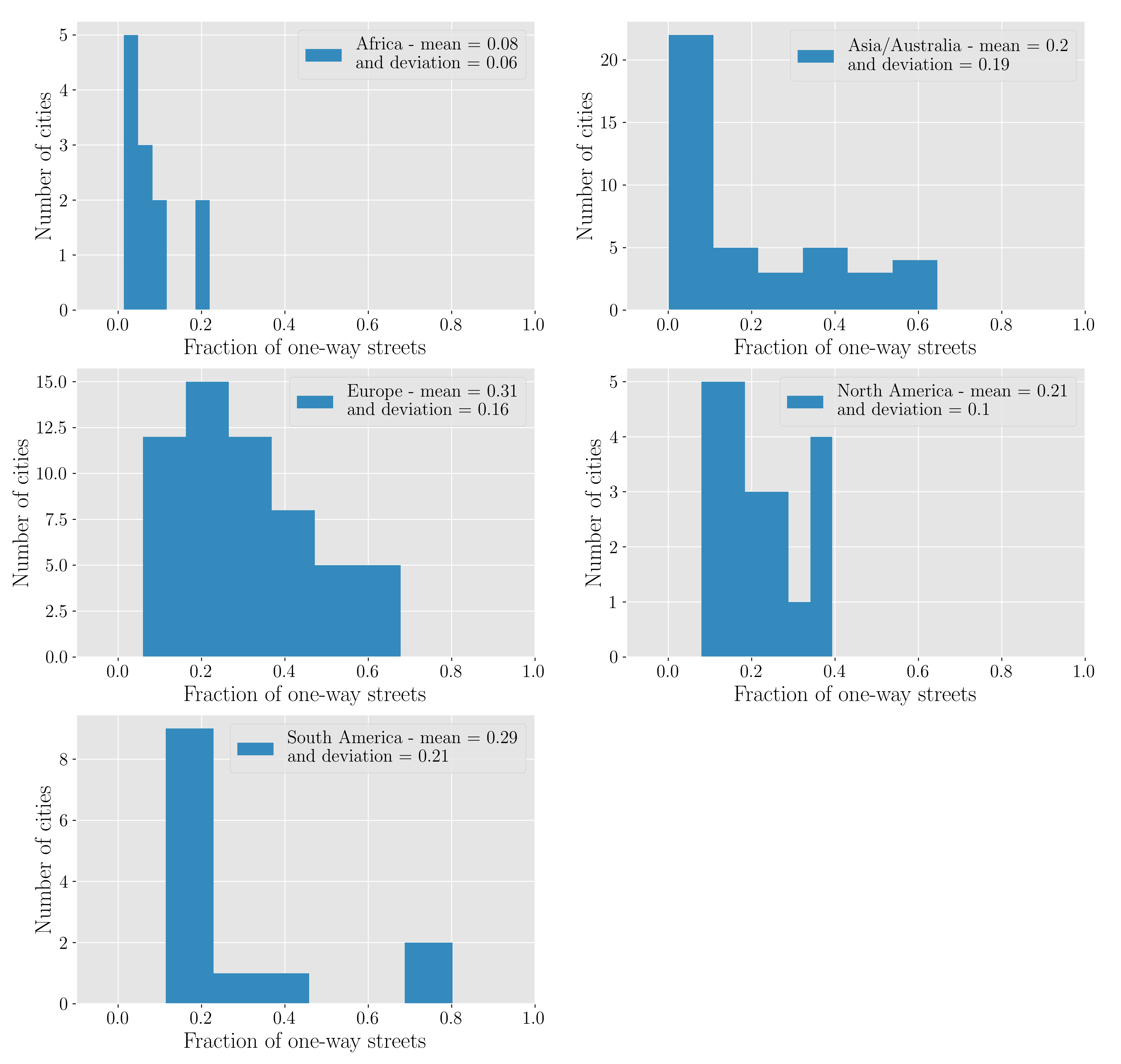
Figure 1: Distribution of the fraction $p$ of one-way streets for the five continents (the fraction is defined as the total length of one-way streets over the total length of the network).

The occurrence of one-way streets seems thus to be connected to more complex street plans Boeing:2019 .

We denote by $d_{G}(i,j)$ the shortest path distance from node $i$ to node $j$ on the undirected graph $G$ and $d_{\vv{G}}(i,j)$ the corresponding quantity for the mixed graph denoted by $\vv{G}$ (when one-ways are taken into account). The average detour due to one-ways is then defined as $\overline{\eta}=\frac{1}{N(N-1)}\sum_{(i,j)\in G}\frac{d_{\vv{G}}(i,j)}{d_{G}(i,j)}-1$. Figure 2a shows how the average detour increases with the fraction of one-way streets $p$ in the dataset of world cities we use. We first observe that the detour increases roughly linearly with the fraction of one-ways (a power law fit gives an exponent of 0.8) and that most cities have an average detour less than $10\%$. We also note that there is a large dispersion of this detour for a given value of the one-way fraction. For example, for $p\approx 0.6$ the detour varies from about $6\%$ for Singapore up to $15\%$ for Beirut (and even $5\%$ for $p=0.7$ for Buenos Aires), showing that the impact on shortest paths depends strongly on the precise location of one-ways. Furthermore, we can separate the impact of one-ways on various distances by defining the detour profile given by

$$\eta(d)=\frac{1}{N(N-1)}\sum_{(i,j)\;s.t.\;d_{G}(i,j)=d}\frac{d_{\vv{G}}(i,j)}{d_{G}(i,j)}-1$$ (1)

We observe for various cities on Fig. 2b that $\eta(d)$ roughly decreases as a power law of the form $\eta(d)\sim d^{-\theta}$ demonstrating the impact of one-way streets even for large distance (in this figure, the distance is normalized by its maximum value for each city). In particular, we note that if on average the detour due to one-way streets is of the order of 10%, which seems small, detours at short distances may be significantly higher (up to the order of 100%). Also, even if $10\%$ is small at an individual level, this has a non-neglibible effect in terms of time cost and congestion at the city scale when summed over all car users.

The exponent $\theta$ does not seem to be universal and ranges between $0.2$ and $0.8$ for different cities. We note that we expect in general $\theta\in[0,1]$ where the upper-bound $\theta=1$ corresponds to the case where one-way streets create a constant detour in the directed network, implying $d_{\vv{G}}(i,j)=C+d_{G}(i,j)$ and therefore $\eta(d)\sim 1/d$. The case $\theta=0$ corresponds to the situation where the detour is proportional to the distance traveled: $d_{\vv{G}}(i,j)\propto d_{G}(i,j)$ implying $\eta(d)\sim const$. In any case, this slow decrease of $\eta(d)$ with $d$ signals the long-range effect of one-ways on shortest paths.

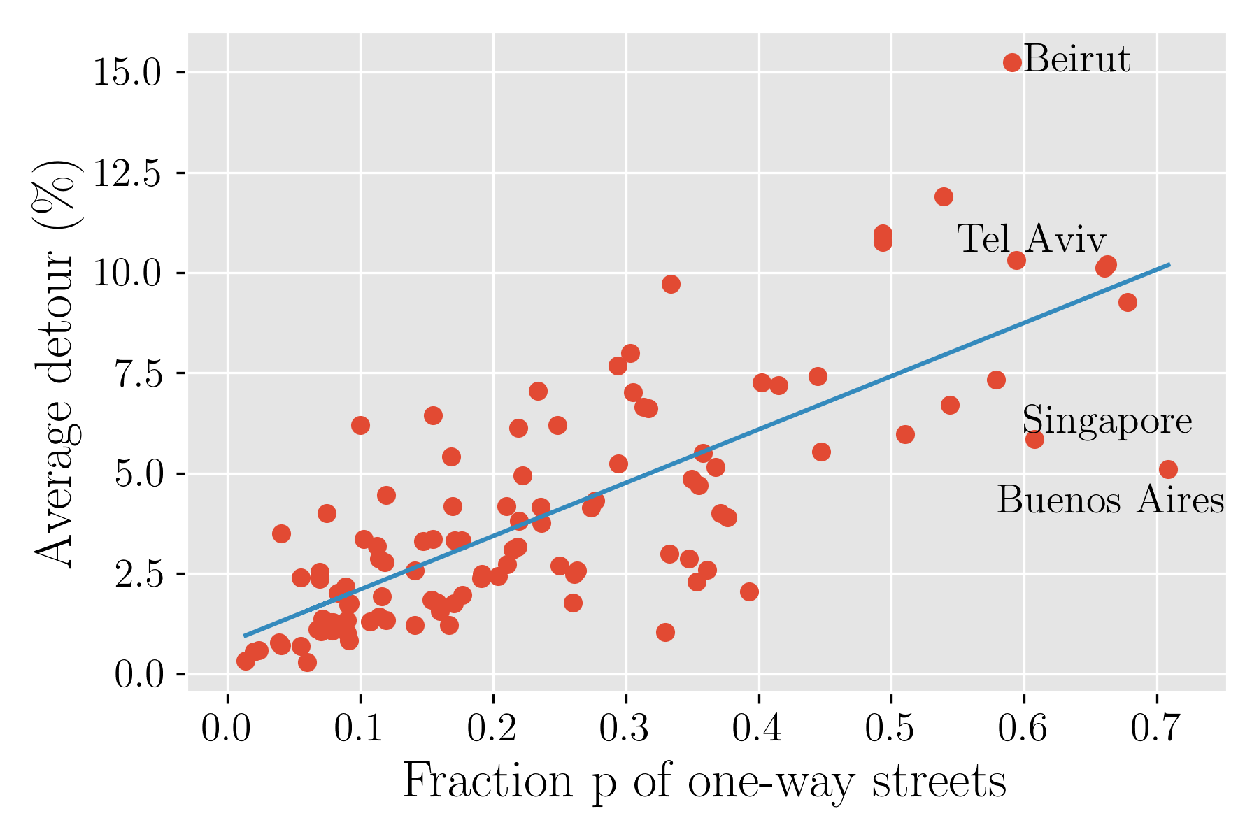
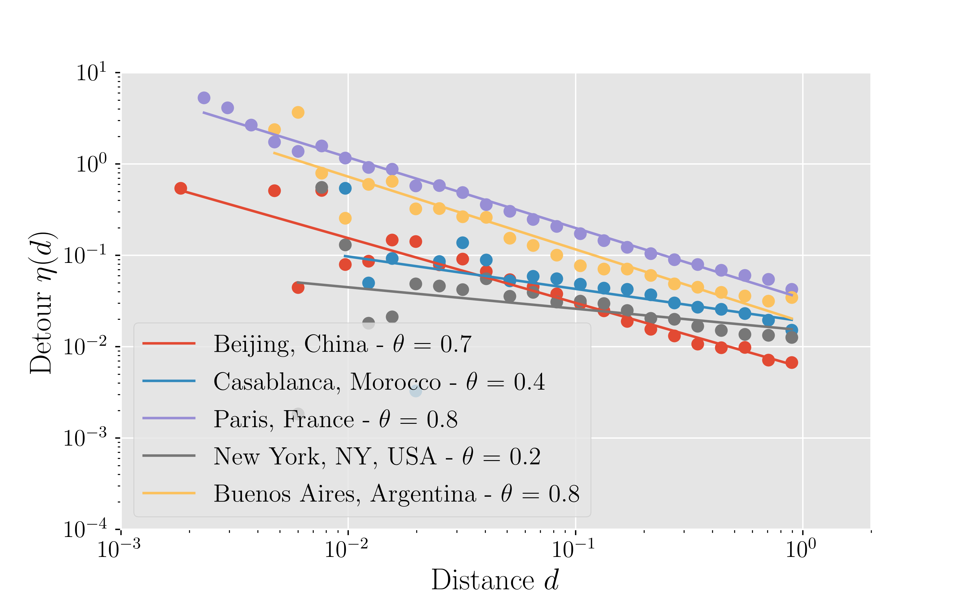
Figure 2: (a) Distribution of the average detour ($\%$) as a function of fraction $p$ of one-way streets for 146 world cities ($R^{2}=0.59$). (b) For five selected cities in the world, we plot the average detour $\eta(d)$ due to one-way streets for a trip of distance $d$ as a function of $d$ (normalized by the maximum distance obtained for each city). The detour can be fitted by a power $\eta(d)\sim d^{-\theta}$. We find that $\theta$ differs from one city to another and ranges roughly from $0.2$ to $0.8$. In particular, small exponent values (such as in the case of NYC) might be correlated with the presence of very long one-way streets leading to a large detour even at very large spatial scales. We have $R^{2}=0.87$ for Beijing, $R^{2}=0.25$ for Casablanca, $R^{2}=0.99$ for Paris, $R^{2}=0.12$ for NYC and $R^{2}=0.90$ for Buenos Aires.

II.2 Betweenness centrality

Cars have to follow the direction of links and consequently one-way streets govern the spatial structure of traffic. The theoretical question is then to understand what happens to the patterns of shortest paths when we turn an undirected link into a one-way street. This can for instance be measured by comparing the betweenness centrality (BC) of nodes (see for example Kirkley:2018 ; Barthelemy:2018 and references therein). We denote by $g_{G}(i)$ the BC of node $i$ on the graph $G$ defined as

$$g_{G}(i)=\frac{1}{{\cal N}}\sum_{s\neq t}\frac{\sigma_{st}(i)}{\sigma_{st}}$$ (2)

where $\sigma_{st}$ is the number of shortest paths from node $s$ to node $t$ and $\sigma_{st}(i)$ the number of these shortest paths that go through node $i$. The quantity ${\cal N}$ is a normalization that we choose here ${\cal N}=(N-1)(N-2)$. We denote by $g_{\vv{G}}(i)$ the BC of node $i$ when we include one-ways, and we analyze the relative variation $\Delta=(g_{\vv{G}}(i)-g_{G}(i))/g_{G}(i)$. In the case of Paris for example, we find that $53\%$ of the nodes have a smaller BC ($\Delta<0$) due to one-way streets with $27\%$ of them having less than half the undirected BC and $3\%$ less than $10\%$. For the other $47\%$ with $\Delta>0$ the BC is increased, more than doubled for $31\%$ of them and the BC is ten times higher in $3\%$ of cases. We thus observe here the dual effect of one-way streets: certain nodes are preserved and experience a reduced traffic while this simultaneously create bottlenecks where the BC can be very large. More generally, we observe (see Fig 3) that the distribution of $\Delta$ is not symmetric (with a global average of $\sim 0.59$) and skewed towards positive values indicating that the bottlenecks due to the deviated traffic can be extremely busy.

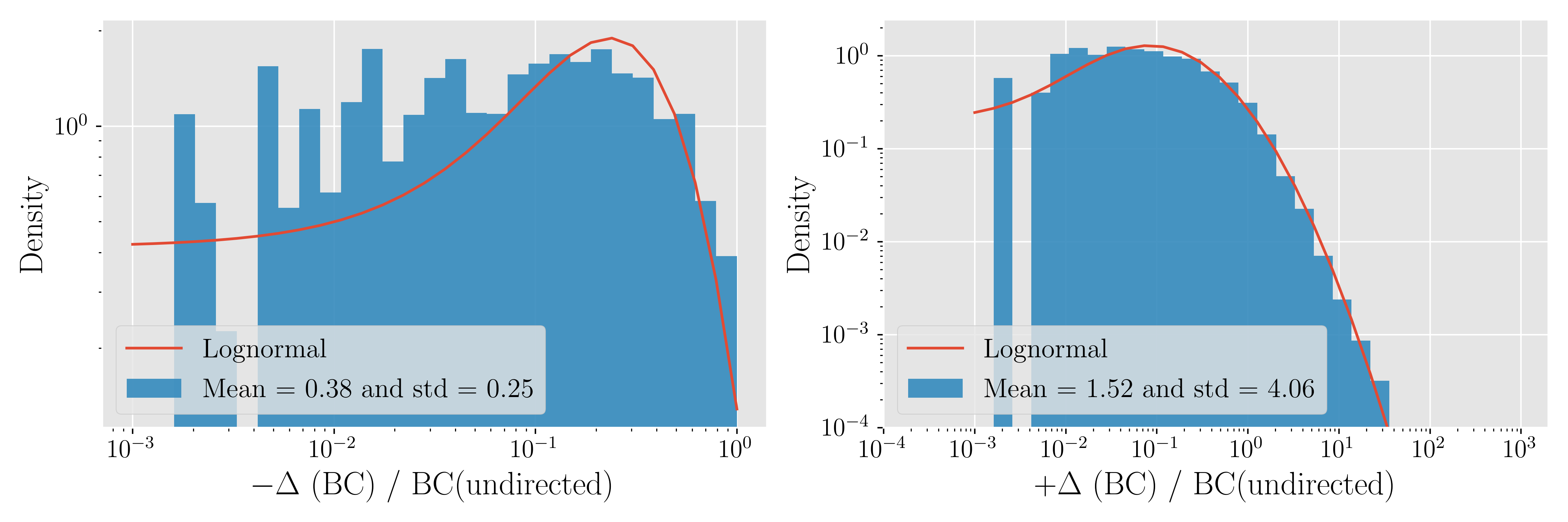
Figure 3: Distribution of the relative variation $\Delta$ of the betweenness centrality (BC) due to one-way streets in the Parisian network for negative (the BC decreases) and positive values of $\Delta$ (the BC increases with one-ways). Both distributions can be fitted by a lognormal and parameters are: $\mu=0.38$, $\sigma=0.25$ (negative values) and $\mu=1.52$ and $\sigma=4.06$. The distribution for positive values of $\Delta$ is much broader with large values of the relative variation of the BC demonstrating the creation of critical bottlenecks in the network. (a) For $53\%$ of the nodes, we have $\Delta<0$ which correspond to nodes having a smaller BC due to one-way streets. In this case, $27\%$ of the nodes have less than half the undirected BC and $3\%$ less than $10\%$. (b) For $47\%$ of nodes, the BC is increased by one-way streets. For $31\%$ of these nodes, their BC doubled or more, and for $3\%$ it is ten times larger.

II.3 Strongly connected component

The strongly connected component (SCC) in the directed graph is the set of nodes such that there is a directed path connecting any pairs in it Roberts:1978 . We note that for a weakly connected graph such as the street network, there is one SCC only. We first show (see Fig. 4 left column) the distribution of degrees of nodes (junctions) in five different cities in the world, whose fraction $p$ of one-way streets ranges from $19\%$ to $71\%$ (see Table 1). As we could anticipate, we note significant differences in the degree distribution between old cities like Paris or Beijing where and newer cities like New York City, where important areas are in the form of a square grid. Except in the cases of Casablanca and Beijing, one-way streets represent more than half of the total length of the network. It is even more pronounced in the case of square-gridded cities such as Manhattan where the percentage of one-ways is $69\%$ (with many east/west or north/south oriented avenues and streets) which probably correspond to the need for decreasing congestion and for simplifying the navigation in the city. For each of these cities, we keep the underlying bidirectional structure of the graph (that we call the substrate of the real network) and we vary the fraction $p$ of one-way streets from $0$ to $1$ by randomly turning a share $p$ of streets into one-way streets (and $1-p$ is therefore the remaining fraction of undirected links representing two-ways streets). In that process, bidirectional streets in the real world may be turned into one-way streets while one-way streets may be bidirectional. Hence, for each value of $p$, we randomly allocate one-way streets (with random orientation) and compute the size $S$ of the strongly connected component, normalized by the number $N$ of nodes. We construct many realizations of this process allowing us to compute statistical properties.

This measure of $S/N$ enables us to understand how many streets can be randomly turned into one-way streets before parts of the city become disconnected. We compare in Fig. 4 (right column) the resulting curve for the same process on regular lattices of 3-point junctions (honeycomb lattice) and 4-point junctions (square lattice). For every city, we observe an abrupt percolation-like transition for the SCC size when the fraction of random one-way streets increases. We notice that for each city the real share $p_{real}$ (represented by the star) of one-way streets is below the transition threshold and that in general $({S/N})_{real}\approx 1$, which means that - fortunately - cities are not disconnected in the real life. This is expected for practical reasons and Robbins’ theorem Robbins:1939 states the existence of such a solution whatever the fraction of directed links. We note, however, that this solution is statistically not frequent and may be very far from the average of ${S/N}$ over all random configurations at share $p_{real}$.

Figure 4: (Left column): The degree distribution of junctions for 5 different cities from 5 different continents. The average degree for these cities is $\langle k\rangle\sim 3.4$ (Casablanca), $\sim 3.1$ (Beijing), $\sim 3.5$ (New York), $\sim 3.4$ (Paris), $\sim 3.7$ (Buenos Aires). The most common junction is a 3-points fork in Casablanca, Paris and Beijing, while 4-points crossroads are more frequent in New York City and Buenos Aires. (Right column) The blue points are obtained by picking a fraction $p$ of streets in the underlying bidirectional structure of the city (that we call the substrate of the real network) and turning them into one-way streets. In that statistical process, bidirectional streets in the real world may be turned into one-way streets while one-way streets may be bidirectional. We then plot the largest strongly connected component size ($S$) in the total network normalized by the number $N$ of nodes as a function of $p$. Results are obtained for 10 different disorder realizations.

III Percolation analysis

III.1 Percolation and digraphs. The model.

These empirical results bring us to study in more depth this percolation-like transition observed for mixed graphs. We first note that this problem is different from the rare results available for digraphs (see for example Luczak:1990 ; Newman:2001 ; Schwartz:2002 ; Doro:2001 ; Boguna:2005 ; Bianconi:2008 and references therein). For example, similarly to the Erdős-Renyi transition Erdos:1960 , adding directed links to a digraph leads to a transition for the strongly connected component Luczak:1990 : for $M/N>1$, there is an infinite SCC ($M$ is the number of directed arcs, and $N$ the number of nodes). The control parameter is then the number of edges which are all directed. Other studies generalized percolation in random fully directed – generally uncorrelated – networks Newman:2001 ; Schwartz:2002 ; Doro:2001 ; Boguna:2005 but whose results cannot be directly applied to regular lattices due to the strong degree correlations and the non-random nature of links. Our model is also different from the well-known model of directed percolation in statistical physics Obukhov:1980 ; Broadbent:1957 where a preferred direction is chosen for all bonds on a regular lattice and which defines a universality class different from usual percolation.

This type of percolation model was introduced by Redner in a series of papers Redner:1982a ; Redner:1982b ; Redner:1982c as the random resistor diode percolation, and was studied further in Inui:1999 ; Janssen:2000 ; Zhou:2012 ; DeNoronha:2018 . In the more general version of this model defined on lattices, bonds can be absent, be a resistor that can transmit an electrical current in either direction along their length, or diodes that connect in one direction only. The general phase diagram was discussed in Redner:1982a ; Redner:1982b using real-space renormalization arguments which predict fixed points associated with standard percolation, directed percolation, and other new transitions. The crossover between isotropic and directed percolation was further studied in Inui:1999 ; Janssen:2000 ; Stenull:2001 ; Zhou:2012 . In relation to the problem discussed here, Redner Redner:1982a observed a ‘reverse percolation’ transition from a one-way connectivity in a given direction to a two-way (isotropic) connectivity when connected paths oriented opposite to the diode polarization begin to span the lattice. This transition from a connected component to a strongly connected component corresponds to what we observe here.

The model discussed in this paper was previously considered in DeNoronha:2018 where critical exponents are computed on isotropically directed lattices where bonds can be either absent, directed or undirected (in Hillebrand:2018 the authors considered some properties in the critical case). The particular case where bonds are either undirected or directed (but cannot be absent) is the specific case that applies to road networks and that we will focus on. We recall here the precise definition of this model. We consider a mixed graph $\vv{G}$ whose edges can be either directed or undirected. As in the previous section, we denote by $p$ the fraction of directed edges and the limits $p=0$ and $p=1$ correspond then to the undirected and the fully directed graph, respectively. We assume that the directed links have a random direction without any bias (i.e. each direction has a probability $1/2$). We vary the fraction $p$ and measure various quantities and we will consider regular lattices such as the square and the honeycomb lattices.

III.2 Detour properties

We will first consider the average detour on the honeycomb lattice and observe that it increases with $p$ (Fig. 5 for Paris.

Figure 5: Average detour $\overline{\eta}$ as a function of the fraction $p$ of randomly chosen one-way streets in the city of Paris (France). In this statiscal process, the detour increases with the fraction $p$. We note, however, that the empirical detour in the real world (indicated by a star symbol) remains below the result expected from a random uniform distribution of one-way streets. This indicates that the actual choice of one-way streets in Paris is far from what would be obtained by a random choice of one-way streets and favors small detours. We compare these results to the obtained for a honeycomb lattice, whose degree distribution is close the Paris.

We also see in Fig. 5 that the real detour is below the result obtained for a random distribution of one-way streets (similar results are obtained for other cities). This demonstrates the importance of the precise location of one-ways that can affect in very different ways the shortest paths statistics.

For the honeycomb lattice (Fig. 6), the average detour $\eta(d)$ due to directed links for a trip of distance $d$ scales as a power-law of $d$ with $\eta(d)\sim d^{-\theta}$ (the quantity $d$ is here normalized by its maximum value). We find $\theta=0.5\pm 0.1$ as shown in the data collapse of Fig. 6(a). More precisely, we also show that the relation is of the form $\eta(d)=A(p)d^{-1/2}$ that remains valid for all $p$ and with $A(p)\sim p^{2.3}$ (see Fig. 6b). This result in $1/\sqrt{d}$ suggests the possibility of an argument relying on the sum of random quantities leading to $d_{\vv{G}}(i,j)-d_{G}(i,j)\sim\sqrt{d}$.

Figure 6: Average detour for the honeycomb lattice. (a) We show the quantity $\eta(d)\sqrt{d}$ versus d normalized by its value at $d=0.1$. The curves collapse onto a single one independent from d and the observed discrepancies for $d$ close to $1$ and $d$ small come from finite-size effects. (b) The collapse suggest a form $\eta(d)=A(p)d^{-1/2}$, and a power law fit gives $A(p)\sim p^{\gamma}$ with $\gamma\approx 2.3$ ($R^{2}=0.94$). We, however, observe discrepancies at large $p$.

III.3 Percolation threshold

In the following, we will focus on the size of the SCC and related properties. In order to distinguish the new transition from the usual percolation we will use the term ‘SCC-percolation’ when needed. Similarly to classical percolation Sykes:1964 ; Kesten:1982 ; Sahimi:1994 ; Callaway:2000 ; Christensen:2005 ; wiki ; Stauffer:2018 , we denote by $P_{\infty}$ the probability to belong to the strongly connected component and which will be the order parameter. We observe numerically (over $1000$ runs) that both lattices exhibit a phase transition (see Fig. 8 and 9) at a percolation threshold $p_{c}$ above which the size of the SCC is negligible. We determine the percolation threshold $p_{c}(L)$ for a finite lattice of linear size $L$ using the method described in Yonezawa:1989 . In order to determine the percolation threshold numerically, we define the threshold $p_{c}(L)$ for a finite lattice of linear size $L$ as the fraction of directed graphs for which the probability $P(L)$ to observe a strongly connected cluster connecting two opposite sides of the system is $0.5$ Yonezawa:1989 . In practice, we compute $p_{c}(L)$ as the average threshold between the last time such that $P(L)>0.5$ and the first time such that $P(L)<0.5$ when $p$ increases. Having the threshold $p_{c}(L)$ for different sizes $L$, we use the classical ansatz Yonezawa:1989

$$p_{c}(L)=p_{c}(\infty)-A/L^{\nu}$$ (3)

where $\nu$ is the exponent that describes the divergence of the correlation length $\xi\sim|p-p_{c}|^{-\nu}$. Using this method, we find for the honeycomb lattice $p_{c}=0.6935\pm 0.0005$ and $p_{c}=0.998\pm 0.002$ for the square lattice (see Fig. 8 and Fig. 9). For honeycomb lattices we thus observe a threshold $p_{c}<1$ while for the square lattice we have $p_{c}=1$. This means here that for a degree equal or larger than $4$, the number of different paths between any pair of points is large enough so that the SCC is always large. In contrast, for the honeycomb lattice with a degree $k=3$, some nodes can more easily constitute ‘blocking points’ with one-way streets ending at it (see below for a more detailed argument). Interestingly enough, real street networks have an average degree between $3$ and $4$ implying a non-trivial threshold and the corresponding curve to lie between those for the two lattices. The scaling ansatz also gives the value $\nu=1.1\pm 0.2$ (and the same value for the square lattice) which is slightly different from the isotropic percolation value $4/3$.

For this model, de Noronha et al. DeNoronha:2018 proposed a conjecture for computing the percolation threshold which is based on the idea that it is governed by the probability that the nearest-neighbor can be reached from a given site. Using duality arguments, this conjecture can be proven to be exact for the square, triangular, and honeycomb lattices DeNoronha:2018 . For the model where bonds are either undirected or directed (but not absent), this conjecture reads

$$p_{c}=2(1-p_{c}^{0})$$ (4)

where $p_{c}^{0}$ is the corresponding threshold for the usual percolation on the lattice. For the honeycomb lattice, $p_{c}^{0}=1-2\sin\pi/18$ which implies $p_{c}=4\sin\pi/18\approx 0.6926...$ in agreement with our numerical estimate. This conjecture was tested on both the honeycomb and square lattices only and we tested it on real-world random graphs for different cities. We show the results in Table 2.

City	$p_{c}(SCC)$	$p_{c}=1-\frac{1}{2}p_{c}(SCC)$	$p_{c}$ (measured)
Beijing	$0.63$	$0.685$	$0.67(3)$
Casablanca	$0.73$	$0.635$	$0.62(3)$
Paris	$0.78$	$0.61$	$0.57(3)$
NYC	$0.77$	$0.615$	$0.57(3)$
Buenos Aires	$0.88$	$0.56$	$0.52(3)$

Table 2: We show here the SCC percolation threshold for different cities ($p_{c}(SCC)$), the percolation threshold predicted using the conjecture Eq. 4 proposed in DeNoronha:2018 , and the measured threshold.

We observe that there is a good agreement between the value predicted by the conjecture Eq. 4 and our direct measure for different cities: the conjecture seems to be correct for these random graphs (within our error bars).

This conjecture shows that once $p_{c}^{0}$ is smaller than $1/2$, there is no transition. For a regular lattice of degree $k$ (which is $k=2d$ for a hypercubic lattice in dimension $d$), we can then ask what is the value of $k$ above which there is no transition anymore. The percolation threshold is obviously an increasing function of the lattice degree $k$, as it is easier to find a strongly connected component on graphs with more neighbors, and there seems to be no transition for lattices with average degree larger than $4$. It is easy to show that $p_{c}=0$ for the one-dimensional lattice (which corresponds to a regular lattice with degree $k=2$). We propose the following approximation in order to understand how the threshold varies with the degree $k$ in a regular lattice. We adapt to our case the argument proposed in Schwartz:2002 : we assume that a node has an incoming link and we compute its average outdegree $\langle k_{o}\rangle$ (which varies from $0$ to $k-1$, we do not take into account the incoming link here). The notations used are defined in Fig. 7.

Figure 7: Notations: a node of degree $k$ has an incoming link and $k-1$ outgoing links. Among those, we have $m$ outgoing links, $n-m$ incoming links and $k-1-n$ bidirectional edges.

The probability of having the links defined by $(n,m)$ is given by

$$p_{nm}=\left(\frac{p}{2}\right)^{n}(1-p)^{k-1-n}$$ (5)

We take into account that the incoming link can be either undirected (with probability $1-p$) or directed and incoming with probability $p/2$ leading to a prefactor $p/2+1-p$. The outdegree for the configuration defined by $n$ and $j$ is $k-1-n+m$. Considering also the combinatorial factors, we obtain

$$\langle k_{o}\rangle =\sum_{n=0}^{k-1}\left(\frac{p}{2}\right)^{n}(1-p)^{k-1-n}\sum_{m=0}^{n}\binom{k-1}{m}\binom{k-1-m}{n-m}$$ (6)

$$\times(k-1-n+m)\left[\frac{p}{2}+1-p\right]$$ (7)

These sums can easily be computed and we find

$$\langle k_{o}\rangle=\left(1-\frac{p}{2}\right)^{2}(k-1)$$ (8)

The percolation condition is then $\langle k_{o}\rangle\geq 1$ which means that a directed path can go through this node which is a necessary condition for belonging to the SCC. Writing $\langle k_{o}\rangle=1$ then gives the percolation threshold

$$p_{c}(k)=2\left(1-\frac{1}{\sqrt{k-1}}\right)$$ (9)

which is valid in the interval $[2,5]$. This approximate formula gives the exact result $p_{c}(k=2)=0$ and $p_{c}(k\geq 5)=1$. The latter is obviously an approximation but it is in agreement, at least qualitatively with our numerical results. It however overestimates - as expected for a necessary but not sufficient condition - the degree above which $p_{c}=1$, and it would be interesting to find how to modify this argument in order to recover the numerical result $p_{c}(k=4)=1.0$.

III.4 Critical exponent estimates: a new universality class

The critical exponents for this model were already estimated in DeNoronha:2018 and we determine them independently for both the honeycomb (Fig. 8) and the square lattices (Fig. 9). In particular, in DeNoronha:2018 it is assumed that the exponent $\nu$ is the same as in isotropic percolation and given by $\nu=4/3$. We replaced here this assumption by the scaling ansatz Eq. 3 form for the percolation threshold.

Below the percolation threshold, the order parameter scales as $P_{\infty}\sim|p-p_{c}|^{\beta}$ and a direct fit (Fig. 8d) gives $\beta=0.26\pm 0.02$ ($0.27\pm 0.02$ for the square). Above the percolation threshold, the maximal cluster size scales as $s_{\max}\sim|p-p_{c}|^{\sigma}$ and at the threshold exactly, the probability $n_{s}$ to belong to a cluster of size $s$ scales as $n_{s}\sim s^{-\tau}$. These classical exponents take here the following values (Fig. 8): $\tau=2.14\pm 0.05$ ($2.11\pm 0.05$ for the square lattice) and $\sigma=0.56\pm 0.05$ (the exponent $\sigma$ is not defined for the square lattice where $p_{c}=1$). We note here that too close to criticality however, finite-size effects become important when the correlation length is of order the system size which reduces the range over which the fit can be made.

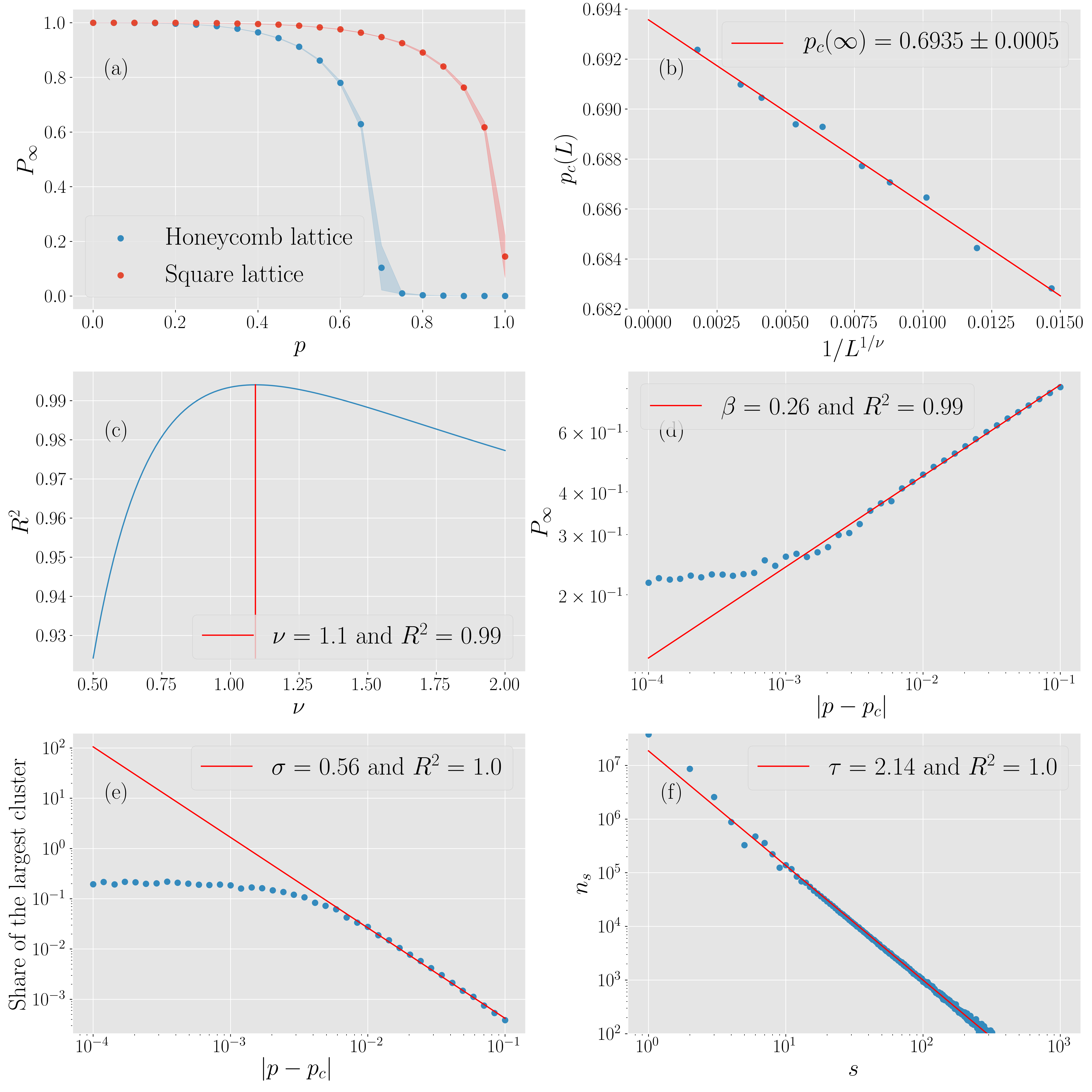
Figure 8: SCC-percolation transition for the mixed honeycomb lattice and the calculation of critical exponents (too close to criticality, finite-size effects become important when the correlation length is of order the system size which reduces the range over which the fit can be made). (a) The probability to belong to the infinite cluster $P_{\infty}$ drops dramatically when the fraction $p$ of one-way streets is close to $0.69$ in the honeycomb lattice and $1$ in the square lattice. (b) Calculation of $p_{c}=0.6935\pm 0.0005$. (c) The regression of the finite-size percolation threshold as a function of $L$ gives the exponent $\nu=1.1\pm 0.2$. (d) Below criticality, the behavior of $P_{\infty}$ with $|p-p_{c}|$ gives the exponent $\beta=0.26\pm 0.02$. (e) Above criticality, the maximal normalized cluster size scales as $s_{max}\sim|p-p_{c}|^{\sigma}$ and we find $\sigma=0.56\pm 0.05$. (f) At criticality, the number of clusters of sizes $s$ scales as $n_{s}\sim s^{-\tau}$ and we find $\tau=2.14\pm 0.05$.

For the square lattice, we obtain the exponents in a similar way (Fig. 9).

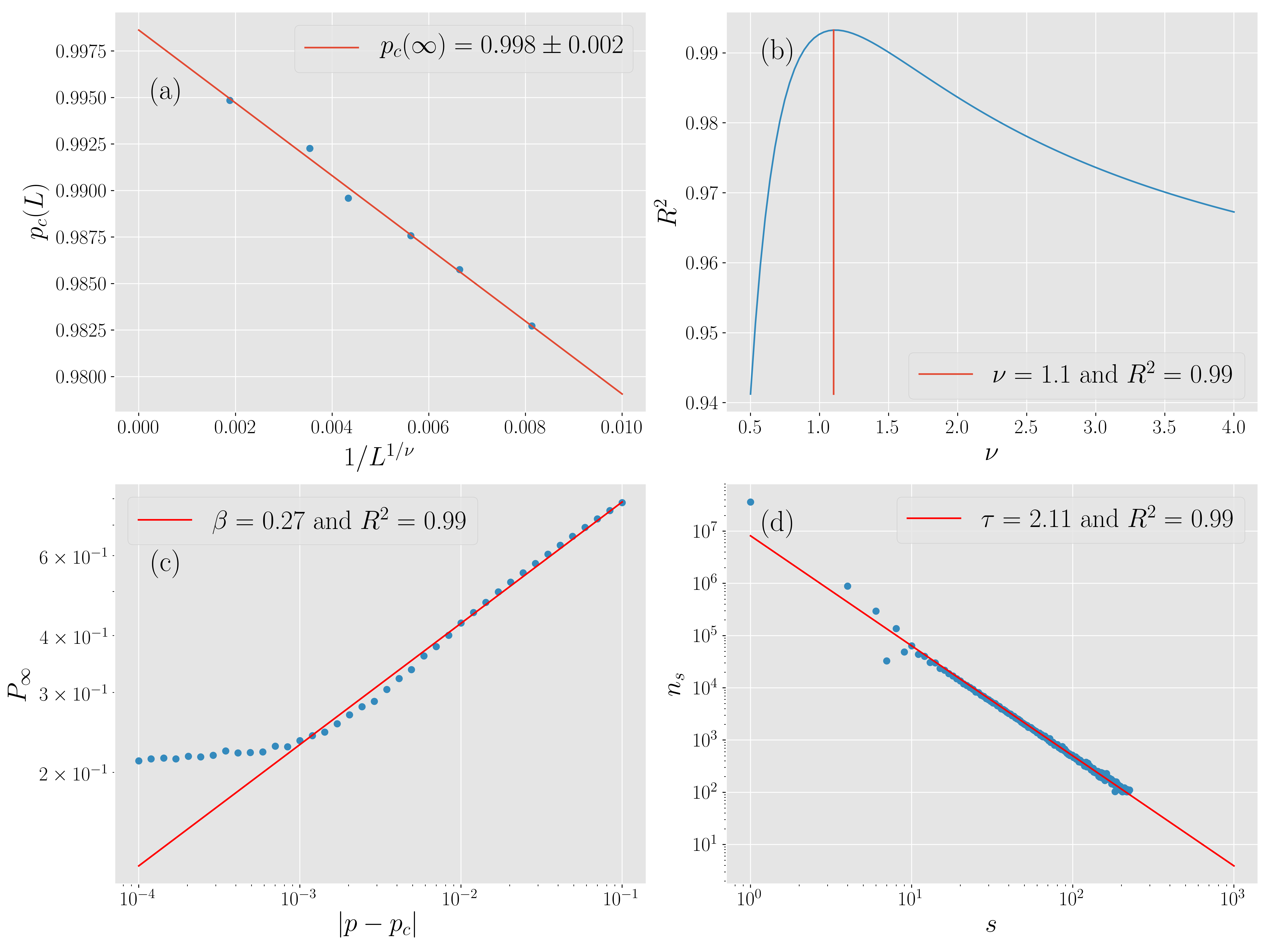
Figure 9: (a) The percolation threshold for an infinite square lattice is calculated as an extrapolation for various finite-size lattices of side size ranging from $L=100$ to $L=1000$. We find $p_{c}=0.998\pm 0.002$. (b) The regression of the finite-size percolation threshold as a function of the linear size also gives the critical exponent $\nu$, and we obtain $\nu=1.1\pm 0.2$. (c) Below criticality, the behavior of $P_{\infty}$ with $|p-p_{c}|$ gives the exponent $\beta=0.26$. (d) At criticality, the number of clusters of sizes $s$ scales as a power-law of the size with critical exponent $\tau$ and we find $\tau=2.14\pm 0.05$.

We note that these exponents satisfy the hyper-scaling relations Christensen:2005 $\tau=d\sigma\nu+1$ and $\beta=(\tau-2)/\sigma$ (where the dimension is here $d=2$), which is expected as these relations are independent from the fact that links are oriented or not. From the classical relations $d_{f}=d/(\tau-1)$ we get for the fractal dimension of the SCC at the threshold the value $d_{f}=1.75\pm 0.08$.

We summarize these results in Table 3. We observe that the exponents are very different from the ones obtained for the percolation on regular undirected lattices or for the directed percolation, in agreement with the results obtained in DeNoronha:2018 and pointing to a new universality class in contrast with the analysis presented in Stenull:2001 ; Zhou:2012 that showed that this model is in the same universality class as standard percolation. There are however some numerical discrepancies (for $\nu$, $\sigma$, and $d_{f}$) between our results and those of DeNoronha:2018 and further work would be needed for a precise determination of the exponents.

Critical	2d	2d directed	Results	This study
exponent	percolation	percolation	of DeNoronha:2018
$\nu$	$4/3$	$1.73$ (parallel)	$4/3$	$1.1\pm 0.2$
		$1.09$ (perp.)
$\beta$	$0.14$	$0.28$	$0.27\pm 0.01$	$0.26\pm 0.02$
$\sigma$	$0.40$	$0.31$	$0.41\pm 0.01$	$0.56\pm 0.05$
$d_{f}$	$1.90$	$1.84$	$1.80\pm 0.01$	$1.75\pm 0.08$
$\tau$	$2.05$	$1.46$	$2.12\pm 0.08$	$2.14\pm 0.05$

Table 3: Critical exponents for standard percolation wiki ; Jensen:1999 compared to directed percolation Deng:2018 , the results obtained in DeNoronha:2018 , and our results for SCC-percolation on mixed graphs.

IV Understanding the transition in disordered real-world networks

Real-life street networks differ from the theoretical square and honeycomb lattices. In particular, the degree distribution of vertices (junctions) in city networks can exhibit different shapes (see Fig. 4 left), either being centered around 3-point junctions - like in Beijing - and hence closer to the honeycomb lattice, or being centered around 4-point junctions – as in Buenos Aires for instance - and closer to the square lattice, or being a combination of both like in New York City. In order to test the effect of disorder on the percolation behavior, we build various graphs starting from regular lattices, and add or remove randomly edges. Removing links from the honeycomb lattice shifts the SCC-percolation threshold towards lower values in a linear way (Fig. 10a) while the average degree $\langle k\rangle$ drops below $3$. When the fraction of removed links is about $35\%$ which corresponds to the standard bond percolation threshold of the regular undirected honeycomb lattice (the exact value is $2\sin\pi/18$ Sykes:1964 ), the giant component vanishes even without directed links (an obvious necessary condition for having a SCC is indeed the existence of a weakly connected giant component). On the contrary, adding random edges to this graph increases the percolation threshold until they are too many edges in the system and the transition does not occur anymore, as there is always a directed path connecting any pair of nodes (Fig. 10b).

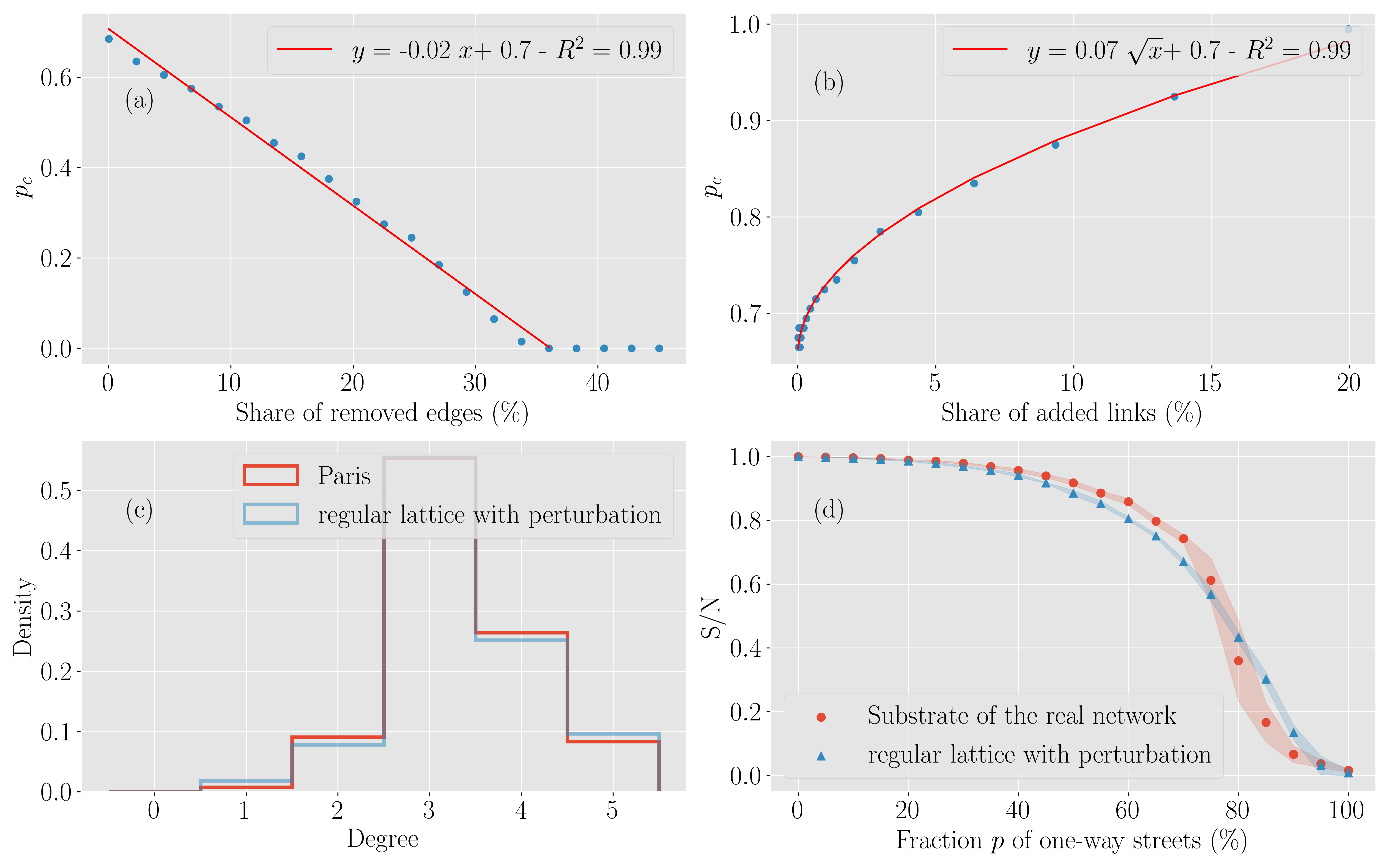
Figure 10: (a) The SCC-percolation threshold decreases linearly with the share of edges removed from the honeycomb lattice. When the fraction of removed links is about $35\%$, the giant component of the undirected honeycomb lattice breaks down and the SCC-percolation threshold is 0. (b) The SCC-percolation threshold increases with the number of edges added to the honeycomb lattice. The behavior is here well fitted by a square root function. (c) Starting from a regular square lattice, we construct various random planar graphs by both addition and removal of edges until the distribution of degrees is close to Paris. (d) On average, we recover the SCC-percolation transition of the Paris real network.

As observed above (Fig. 4 right column), underlying graphs of real-world networks exhibit different non-trivial SCC-percolation behaviors that result from the disorder in their structure. We model these graphs by removal and addition of links in the regular graph. There are several different ways of generating a random planar graph whose distribution of degrees is close a given distribution. To approximate the degree distribution of real world cities, we use the following heuristic algorithm: starting from a regular square lattice, we delete a certain share $\alpha_{4}$ of links for which at least one of the endpoints has degree 4. We then do the same operation by removing a certain share of links $\alpha_{3}$ for which at least one of the endpoints has degree 3, then 2. Finally, we add a share of links $\beta_{4}$ between nodes of degree 4 and other nodes. We then adjust step by step the parameters $\alpha_{1}$, $\alpha_{2}$, $\alpha_{3}$, $\alpha_{4}$ and $\beta_{4}$ until we find a distribution of degrees that is reasonably close to the real one. We test this model on the case of Paris (France) and we construct a random mixed graph whose distribution of degrees is close to the real one: starting from a regular square lattice, we construct various random planar graphs by both addition and removal of edges until the distribution of degrees is close to the empirical one (for Paris here). With this theoretical network, we are able to recover the observed percolation transition of the underlying network of Paris (Fig. 10c and d) not to be confused with the actual choice of one-way streets in Paris, which was proven to be statistically unlikely. We retrieve the transition both at the level of the percolation threshold and the shape of the function (see Fig. 11 for other cities).

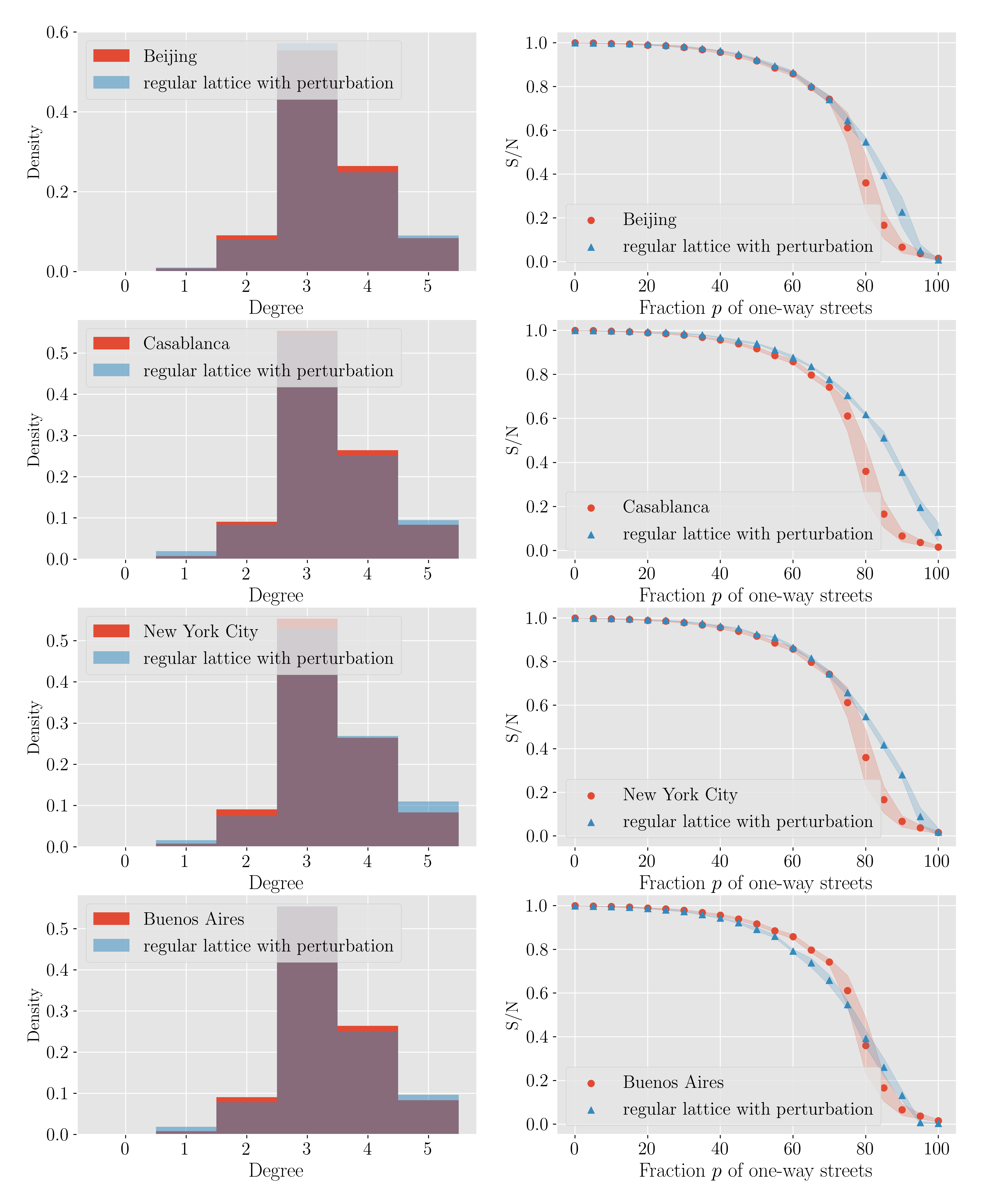
Figure 11: In four cities, starting from a regular square lattice, we construct various random planar graphs by both addition and removal of edges until the distribution of degrees is close to the real one (left panel). On average, we recover the SCC-percolation transition of the corresponding real network (right panel).

These results suggest that the degree distribution is actually the main determinant for the percolation behavior on these real-world graphs. It is important to note that for percolation, bonds are drawn at random, while as noted above, there are correlations between one-way streets locations in real configurations and the degree distribution is not the only determinant in this case.

V Discussion

One-way streets in large cities are of fundamental importance for controlling car traffic with dramatic effects on neighborhoods in terms of pollution and noise. Urban planners have achieved to increase the number of one-way streets in cities while preserving a giant strongly connected component, as ensured by Robbin’s theorem: even if it is a very hard task to do from scratch, adding one-ways by preserving the strong orientation is a working strategy. How to locate one-way streets and their effect on the graph structure were already the subject of a few mathematical studies in graph theory, and we show here that this problem has in addition interesting connections with statistical physics. In particular, this problem naturally leads to a new percolation-like model which belongs to a new universality class. Understanding better this transition on both regular lattices and disordered graphs represents certainly a challenge for theoretical physicists, and might also shed light on the effects of one-way streets in our cities.

Acknowledgements - This paper is dedicated to the memory of Pierre Rosenstiehl who recently passed away. We thank Geoff Boeing for his invaluable help for using OSMnX and Sid Redner for useful discussions about the random resistor-diode network. MB thanks Edouard Brézin for his original suggestion to look at this problem and Fabien Pfaender for discussions at an early stage of this work. This material is based upon work supported by the Complex Systems Institute of Paris Ile-de-France (ISC-PIF). VV thanks the Ecole nationale des Ponts et Chaussées for financial support.

References

- (1) Verbavatz, V. & Barthelemy, M. Critical factors for mitigating car traffic in cities. PLoS one 14, e0219559 (2019).
- (2) Dodman, D. Blaming cities for climate change? An analysis of urban greenhouse gas emissions inventories. Environ. Urban 21, 185–201 (2009).
- (3) Newman, P.G. The environmental impact of cities. Environ. Urban 18, 275–295 (2006).
- (4) Lay, M. A History of the World’s Roads and of the Vehicles That Used Them, Rutgers University Press, 1992.
- (5) Homer, T. The Book of Origins. London: Portrait., 2006.
- (6) Stemley, J.J. One-way streets provide superior safety and convenience. ITE journal 68, 47-50 (1998).
- (7) Venerandi, A., Zanella, M., Romice, O., Dibble, J., Porta, S. Form and urban change–An urban morphometric study of five gentrified neighbourhoods in London. Environment and Planning B: Urban Analytics and City Science 44, 1056-1076 (2017).
- (8) Jiang, B. & Claramunt, C. Topological analysis of urban street networks. Environment and Planning B: Planning and design 31, 151-162 (2004).
- (9) Buhl, J., Gautrais, J., Reeves, N., Solé, R., Valverde, S., Kuntz, P., Theraulaz, G. Topological patterns in street networks of self-organized urban settlements. The European Physical Journal B-Condensed Matter and Complex Systems 49, 513 (2006).
- (10) Strano, E., Viana, M., da Fontoura Costa, L., Cardillo, A., Porta, S., Latora, V. Urban street networks, a comparative analysis of ten European cities. Environment and Planning B: Planning and Design 40, 1071-1086 (2013).
- (11) Xie, F. & Levinson, D. Measuring the structure of road networks. Geographical analysis 39, 336-356 (2007).
- (12) Lammer, S., Gehlsen, B., Helbing, D. Scaling laws in the spatial structure of urban road networks. Physica A: Statistical Mechanics and its Applications 363, 89-95 (2006).
- (13) Strano, E., Nicosia, V., Latora, V., Porta, S., Barthelemy, M. Elementary processes governing the evolution of road networks. Scientific reports 2, 296 (2012).
- (14) Crucitti, P., Latora, V., Porta, S. Centrality measures in spatial networks of urban streets. Physical Review E 73, 036125 (2006).
- (15) Louf, R. & Barthelemy, M. A typology of street patterns. Journal of The Royal Society: Interface 11, 20140924 (2014).
- (16) Kirkley, A., Barbosa, H., Barthelemy, M., & Ghoshal, G. From the betweenness centrality in street networks to structural invariants in random planar graphs. Nature communications, 9, 1-12 (2018).
- (17) Barthelemy, M. Morphogenesis of spatial networks, Cham, Switzerland: Springer International Publishing., 2018.
- (18) Boeing, G. Urban spatial order: street network orientation, configuration, and entropy. Appl Netw Sci. 4 ( 2019).
- (19) Beck, M., Blado, D., Crawford, J., Jean-Louis T., Young, M. On weak chromatic polynomials of mixed graphs. Graphs and Combinatorics, 2013.
- (20) Roberts, F.S. Graph theory and its applications to problems of society, Philadelphia (USA): Society for industrial and applied mathematics (SIAM), 1978.
- (21) Robbins, H.E. A theorem on graphs, with an application to a problem on traffic control. American Mathematical Monthly 46, 281-283 (1939).
- (22) Boesch, F. & Tindell, R. Robbins’s theorem for mixed multigraphs. The American Mathematical Monthly 87, 716–719 (1980).
- (23) Chvatal, V. & Thomassen, C. Distances in orientations of graphs. Journal of Combinatorial Theory, Series B 24, 61-75, 1978.
- (24) OpenStreetMap,2020. [Online]. Available: https://www.openstreetmap.org/#map=6/46.449/2.210
- (25) Boeing, G. OSMnx: New Methods for Acquiring, Constructing, Analyzing, and Visualizing Complex Street Networks. Computers, Environment and Urban Systems 65, 126-139 (2017).
- (26) Hagberg,A., Swart, P., Chult, D.S. Exploring network structure, dynamics, and function using NetworkX. In Proceedings of the 7th Python in Science Conference (2008).
- (27) Csardi, G. & Nepusz, T. The igraph software package for complex network research. InterJournal, Complex Systems, 1695 (2006).
- (28) https://gitlab.iscpif.fr/vverbavatz/digraphs
- (29) Łuczak, T. The phase transition in the evolution of random digraphs. Journal of graph theory 14, 217-223 (1990).
- (30) Newman, M.E., Strogatz, S.H., Watts, D. Random graphs with arbitrary degree distributions and their applications. Physical review E 64, 026118 (2001).
- (31) Schwartz, N., Cohen, R., Ben-Avraham, D., Barabasi, A.-L., Havlin, S. Percolation in directed scale-free networks. Physical Review E 66, 015104 (2002).
- (32) Dorogovtsev, S.N., Mendes, J.F., Samukhin, A.N. Giant strongly connected component of directed networks. Physical Review E 64, 025101 (2001).
- (33) Bogunà, M. & Angeles, S.M. Generalized percolation in random directed networks. Physical Review E 72, 016106 (2005).
- (34) Bianconi, G., Gulbahce, N., Motter, A.E. Local structure of directed networks. Physical Review Letters 100, 118701 (2008).
- (35) Erdős, P. & Rényi, A. On the evolution of random graphs. Publ. Math. Inst. Hung. Acad. Sci 5, 17-60 (1960).
- (36) Obukhov, S.P. The problem of directed percolation. Physica A 101, 145-155 (1980).
- (37) Broadbent S.R. & Hammersley, J.M. Percolation processes: I. Crystals and mazes. Mathematical Proceedings of the Cambridge Philosophical Society 53, 1957.
- (38) Redner, S. Directed and diode percolation. Phys. Rev. B 25, 3242 (1982).
- (39) Redner, S. Exact exponent relations for random resistor-diode networks. Journal of Physics A: Mathematical and General 15, L685 (1982).
- (40) Redner, S. Conductivity of random resistor-diode networks. Phys. Rev. B 25, 5646 (1982).
- (41) Inui, N., Kakuno, H., Tretyakov, A. Y., Komatsu, G., & Kameoka, K. Critical behavior of a random diode network. Phys. Rev. E, 59, 6513 (1999).
- (42) Janssen, H.-K., Stenull, O. Random resistor-diode networks and the crossover from isotropic to directed percolation. Phys. Rev. E, 62, 3173 (2000).
- (43) Stenull, O., and Janssen, H.-K.. Conductivity of continuum percolating systems. Phys. Rev. E 64, 056105 (2001).
- (44) Zhou, Z., Yang, J., Ziff, R. M., & Deng, Y. Crossover from isotropic to directed percolation. Phys. Rev. E, 86, 021102 (2012).
- (45) De Noronha, A. W., Moreira, A. A., Vieira, A. P., Herrmann, H. J., Andrade Jr, J. S., & Carmona, H. A. Percolation on an isotropically directed lattice. Physical Review E, 98, 062116 (2018).
- (46) Hillebrand, F., Lukovic, M., & Herrmann, H. J. (2018). Perturbing the shortest path on a critical directed square lattice. Physical Review E, 98(5), 052143.
- (47) Sykes, M.F. & Essam, J.W. Exact critical percolation probabilities for site and bond problems in two dimensions. Journal of Mathematical Physics 5, 1117–1127 (1964).
- (48) Kesten, H. Percolation theory for mathematicians, Boston: Birkhäuser (1982).
- (49) Sahimi, M. Applications of percolation theory, CRC Press, 1994.
- (50) Callaway, D.S., Newman, M.E., Strogatz, S.H., Watts, D.J. Network robustness and fragility: Percolation on random graphs. Physical Review Letters 85, 5468 (2000).
- (51) Christensen, K. & Moloney, N.R. Complexity and criticality, World Scientific Publishing Company (2005).
- (52) Wikipedia, ”Percolation threshold,” [Online]. Available: https://en.wikipedia.org/wiki/Percolation_threshold [Accessed October 2020].
- (53) Stauffer, D. & Ammon, A. Introduction to percolation theory, CRC press (2018).
- (54) Yonezawa, F., Sakamoto, S., Hori, M. Percolation in two-dimensional lattices. A technique for the estimation of thresholds. Physical Review B 40, 636 (1989).
- (55) Jensen, I. Low-density series expansions for directed percolation: I. A new efficient algorithm with applications to the square lattice. Journal of Physics A: Mathematical and General 32, 5233 (1999).
- (56) Deng, Y. & Ziff, R.M. The elastic and directed percolation backbone, arXiv preprint arXiv:1805.08201 (2018).