Perturbation theory for solitons of the Fokas–Lenells equation : Inverse scattering transform approach

Abstract

We present perturbation theory based on the inverse scattering transform method for solitons described by an equation with the inverse linear dispersion law $\omega\sim 1/k$, where $\omega$ is the frequency and $k$ is the wave number, and cubic nonlinearity. This equation, first suggested by Davydova and Lashkin for describing dynamics of nonlinear short-wavelength ion-cyclotron waves in plasmas and later known as the Fokas–Lenells equation, arises from the first negative flow of the Kaup–Newell hierarchy. Local and nonlocal integrals of motion, in particular the energy and momentum of nonlinear ion-cyclotron waves, are explicitly expressed in terms of the discrete (solitonic) and continuous (radiative) scattering data. Evolution equations for the scattering data in the presence of a perturbation are presented. Spectral distributions in the wave number domain of the energy emitted by the soliton in the presence of a perturbation are calculated analytically for two cases: (i) linear damping that corresponds to Landau damping of plasma waves, and (ii) multiplicative noise which corresponds to thermodynamic fluctuations of the external magnetic field (thermal noise) and/or the presence of a weak plasma turbulence.

I Introduction

Nonlinear evolution equations are widely used as models to describe many phenomena in various fields of physics. The classical examples are well-known universal models in dispersive nonlinear media, such as the Korteweg-de Vries (KdV) and nonlinear Schrödinger (NLS) equations etc. Dodd_book ; Zakharov_book . A common feature of nonlinear evolution equations is the presence of dispersion and nonlinearity which in some cases can effectively balance each other and lead to soliton formation. Note that, generally speaking, most nonlinear equations encountered in practical applications and admitting analytical soliton solutions (most often in the one-dimensional case, but there are examples for the two-dimensional Petviashvili_book and even three-dimensional cases Lashkin2017 ) are not completely integrable in the sense that they do not have $N$-soliton solutions describing the elastic collisions between solitons. Of particular interest are completely integrable equations that are found in real physical applications and are of important practical interest. In plasma physics, for example, such equations are the KdV and NLS equations, derivative nonlinear Schrödinger (DNLS) equation, and the two-dimensional Kadomtsev-Petviashvili equation.

Davydova and Lashkin Lashkin1991 suggested a nonlinear equation governing the dynamics of short-wavelength ion-cyclotron waves in plasmas (the Bernstein modes) Trievel86 ; Akhiezer , which in the one-dimensional case in dimensionless variables has the form

$$u_{xt}-u-i\sigma|u|^{2}u_{x}=0,$$ (1)

where $u(x,t)$ is the slowly varying complex envelope of the electrostatic potential at the ion gyrofrequency, and $\sigma=\pm 1$. Authors of Ref. Lashkin1991 found bright one-soliton solution of Eq. (1) corresponding to vanishing boundary conditions at infinity, and then the same authors (with Fishchuck) presented solutions of Eq. (1) in the form of bright algebraic soliton, dark and anti-dark solitons for the nonvanishing boundary conditions, as well as solutions in the form of nonlinear periodic waves in elliptic Jacobi functions Lashkin1994 . Since the paper Lashkin1991 is not quite widely available in the literature, note that all results of Ref. Lashkin1991 are included in Ref. Lashkin1994 , except for the analysis of the modulation instability of a monochromatic wave of finite amplitude, which is the simplest solution of Eq. (1). As was noted in Ref. Lashkin1994 , the properties of the solitons of Eq. (1) differ from the properties of the solitons of the KdV, NLS and DNLS equations. For example, the bright soliton of Eq. (1) can not be motionless, as well as for the KdV soliton (unlike the NLS and DNLS solitons), but, on the other hand, its velocity does not depend on the soliton amplitude and is an independent parameter unlike the KdV soliton (and like the bright NLS and DNLS solitons). Equation (1) is universal in the sense that it contains only three terms of the second of which corresponds to weak dispersion ($\omega\sim 1/k\ll 1$) and the third to weak (cubic) nonlinearity. Here, $\omega$ and $k$ are the frequency and wave number respectively, where in the linear part $u\sim\exp(i\omega t-ikx)$. The same situation holds for well-known integrable models like the NLS and DNLS equations with the weak dispersion $\omega\sim k^{2}\ll 1$ (and cubic nonlinearity), and KdV equation with $\omega\sim k^{3}\ll 1$ (and quadratic nonlinearity). Note that the weak dispersion and nonlinearity in all cases follow from the physical derivation of the corresponding equations. Later on, Fokas and Lenells showed Fokas1995 ; Lenells2009_Nonlinearity that Eq. (1) is completely integrable and corresponds to the first negative flow of the Kaup–Newell hierarchy of the DNLS equation Kaup1978 , and, therefore, can be solved by the inverse transform scattering (IST) method Zakharov_book . The original version of the equation considered in Ref. Fokas1995 ; Lenells2009_Nonlinearity has been derived as an integrable generalization of the NLS equation using bi-Hamiltonian methods Fokas1995 and then as a model for nonlinear pulse propagation in monomode optical fibers when certain higher-order nonlinear effects are taken into account Lenells2009_derivation . Under this, the corresponding equation in dimensionless variables is

$$iu_{t}-\nu u_{xt}+\gamma u_{xx}+\sigma|u|^{2}(u+i\nu u_{x})=0,$$ (2)

where $\nu$ and $\gamma$ are real constants, $\sigma\pm 1$ and by gauge transformation and a change of variables can be reduced to Eq. (1). Lenells rediscovered Lenells2009_derivation the bright one-soliton solution of Ref. Lashkin1991 without using IST method. Bright $N$-soliton solutions of Eq. (2) were obtained by Lenells in Ref. Lenells2010_N-soliton with the dressing method and for Eq. (1) by the Hirota bilinearization method in Ref. Matsuno_bright2012 . Dark $N$-soliton solutions, which contain dark and anti-dark soliton solutions of Ref. Lashkin1994 , were found by the bilinearization method in Ref. Matsuno_dark2012 . In what follows, we will refer to Eq. (1) as the Davydova-Lashkin-Fokas-Lenells (DLFL) equation.

In reality, in the DLFL equation which describes short-wavelength nonlinear waves in a collisionless plasma, additional terms may be present. They can include effects of dissipation due to finite electric conductivity of plasma when taking into account the ion viscosity, collisionless damping (linear and/or nonlinear Landau damping), influence of external forces (external electric fields under high-frequency plasma heating or particle beams), inhomogeneity of the plasma density and/or the external magnetic field, turbulent environment etc. Trievel86 ; Rukhadze84 . These terms violate the integrability, but being small in many important practical cases, they can be taken into account by perturbation theory. The most powerful perturbative technique, which fully uses the natural separation of the discrete and continuous (i.e. solitonic and radiative) degrees of freedom of the integrable equations, is based on the IST. Perturbation theory based on the IST was first introduced by Kaup Kaup1976 and, independently, by Karpman and Maslov Karpman1977-1 ; Karpman1977 . An important contribution to the development of IST perturbation theory has been made in Ref. Newell1978 . A detailed review of the IST-based perturbation theory for the KdV, focusing NLS, sine-Gordon and Landau-Lifshitz equations is given by Kivshar and Malomed Kivshar1989 . For the defocusing NLS equation with the nonvanishing boundary conditions this was done in Refs. Lashkin_dark2004 , for the modified NLS equation (combining the NLS and DNLS) in Ref.  Doktorov1999 (for only discrete spectrum, using Riemann-Gilbert problem) and in Ref.  Lashkin_MNLS2004 (discrete and continuous spectrum), for the DNLS with the vanishing and nonvanishing boundary conditions in Refs.  Wyller1984 ; Lashkin_DNLS2006 and Ref. Lashkin_J_Phys2007 respectively.

Note that adiabatic equations for soliton parameters can be obtained, generally speaking, without using the IST, and, accordingly, even for non completely integrable equations. The simplest techniques are based on integrals of motion of the corresponding nonperturbed equation or use the variational formalism and they have been applied successfully to various problems in the theory of solitons. However, these methods are suitable for deriving the corresponding evolution equations only in the lowest approximation, when an unperturbed instantaneous shape of one soliton with slowly varying parameters is assumed. They become inapplicable when considering the $N$-soliton solution or when taking into account the effects that arise in higher orders of perturbation theory. On the other hand, only the perturbation theory based on the IST makes it possible to take into account the excitation of continuous (radiative) degrees of freedom, which leads to qualitatively new effects in one-soliton dynamics. These effects include, in particular, perturbation-induced emission of radiation by a soliton, long-range corrections to the soliton’s shape (tails), and the generation of new (secondary) solitons Kaup1976 ; Karpman1977-1 ; Karpman1977 ; Newell1978 ; Bullough1980 ; Kivshar1989 ; Lashkin_dark2004 . In addition, the IST formalism allows one to obtain a criterion of applicability of the adiabatic approach Newell1978 ; Bullough1980 ; Kivshar1989 ; Lashkin_dark2004 ; Ablowitz_dark2011 .

The aim of this paper is to develop a perturbation theory based on the IST for Eq. (1) and to investigate bright soliton propagation in the presence of a perturbation. The perturbed equation is written in the form

$$u_{xt}-u-i\sigma|u|^{2}u_{x}=p[u,u^{\ast}],$$ (3)

where the perturbation is represented by the term $p[u,u^{\ast}]$.

The paper is organized as follows. In section  II we review a theory of the scattering transform for the linear eigenvalue problem associated with the DLFL equation and calculate the corresponding $N$-soliton Jost functions. In section  III integrals of motion are written in terms of the discrete and continuous scattering data. Evolution equations for the scattering data in the presence of perturbations are derived in Sec.  IV. As an application of the presented theory, two cases: (i) linear damping that corresponds to Landau damping of plasma waves, and (ii) multiplicative noise which corresponds to fluctuations of the external magnetic field or the presence of a weak plasma turbulence are considered in Sec.  V . The conclusion is made in Sec.  VI.

Regarding notations, we will use the stars for complex conjugation (for matrices - elementwise). The Pauli matrices are

$$\sigma_{1}=\begin{pmatrix}0&1\\ 1&0\end{pmatrix},\quad\sigma_{2}=\begin{pmatrix}0&-i\\ i&0\end{pmatrix},\quad\sigma_{3}=\begin{pmatrix}1&0\\ 0&-1\end{pmatrix}.$$ (4)

II Inverse scattering transform for the DLFL equation

Equation (1) can be written as the compatibility condition

$$U_{t}-V_{x}+[U,V]=0,$$ (5)

of two linear matrix equations Lenells2009_Nonlinearity , where $M(x,t,\lambda)$ is a $2\times 2$ matrix-valued function and $\lambda$ is a complex spectral parameter

$$M_{x}=UM,$$ (6)

$$M_{t}=VM,$$ (7)

and

$$U=-i\lambda^{2}\sigma_{3}+\lambda Q_{x},\,\,\,\,Q=\begin{pmatrix}0&u\\ \sigma u^{\ast}&0\end{pmatrix}$$ (8)

$$V=\frac{i}{4\lambda^{2}}\sigma_{3}-\frac{i}{2\lambda}\sigma_{3}Q+\frac{i}{2}\sigma_{3}Q^{2},$$ (9)

The Jost solutions $M^{\pm}(x,t,\lambda)$ of Eq. (6) for real $\lambda^{2}$ and for some fixed $t$ ($t$-dependence will be omitted for now) are defined by the boundary conditions

$$M^{\pm}(x,\lambda)\rightarrow E\equiv\exp(-i\lambda^{2}\sigma_{3}x)$$ (10)

as $x\rightarrow\pm\infty$. Since $\mathrm{Tr}\,U=0$, these boundary conditions guarantee that $\mathrm{det}\,M^{\pm}=1$ for all $x$. The matrix Jost solutions $M^{\pm}$ can be represented in the form $M^{-}=(\varphi,-\tilde{\varphi})$ and $M^{+}=(\tilde{\psi},\psi)$, where $\varphi$ and $\psi$ are independent vector columns. The scattering matrix $S$

$$S(\lambda)=\begin{pmatrix}a(\lambda)&-\tilde{b}(\lambda)\\ b(\lambda)&\tilde{a}(\lambda)\end{pmatrix},$$ (11)

with $a\tilde{a}+b\tilde{b}=1$ relates the two fundamental solutions $M^{-}$ and $M^{+}$

$$M^{-}(x,\lambda)=M^{+}(x,\lambda)S(\lambda),$$ (12)

so that

$$\varphi=a\tilde{\psi}+b\psi,$$ (13)

$$\tilde{\varphi}=-\tilde{a}\psi+\tilde{b}\tilde{\psi}.$$ (14)

It follows from Eqs. (6) and (12) that matrices $M^{\pm}$ and $S$ have the parity symmetry properties,

$$M^{\pm}(x,\lambda)=\sigma_{3}M^{\pm}(x,-\lambda)\sigma_{3},\,\,S(\lambda)=\sigma_{3}S(-\lambda)\sigma_{3},$$ (15)

and the conjugation symmetry properties

$$M^{\pm}(x,\lambda) =\sigma_{1}M^{\pm\ast}(x,\lambda^{\ast})\sigma_{1},\quad\,\mathrm{if}\,\,\,\sigma=1,$$ (16)

$$M^{\pm}(x,\lambda) =\sigma_{2}M^{\pm\ast}(x,\lambda^{\ast})\sigma_{2},\quad\,\mathrm{if}\,\,\,\sigma=-1,$$ (17)

$$\tilde{a}(\lambda) =a^{\ast}(\lambda^{\ast}),\quad\,\tilde{b}(\lambda)=-\sigma b^{\ast}(\lambda^{\ast}).$$ (18)

The coefficients $a(\lambda)$ and $b(\lambda)$ are

$$a(\lambda)=\mathrm{det}\,(\varphi,\psi),\,\,\,b(\lambda)=\mathrm{det}\,(\tilde{\psi},\varphi).$$ (19)

Taking into account the boundary conditions Eq. (10), the corresponding integral equations for $M^{\pm}$ can be obtained from Eq. (6)

$$M^{\pm}(x,\lambda)=E(x,\lambda)-\lambda\int_{x}^{\pm\infty}E(x-y,\lambda)Q_{y}(y)$$

$$\times M^{\pm}(y,\lambda)\,dy.$$ (20)

The standard analysis of these Volterra-type integral equations yields the expressions for the Jost solutions at $\lambda=0$,

$$M^{+}(x,0)=M^{-}(x,0)=E(x,0),$$ (21)

and the asymptotics at $\lambda\rightarrow\infty$

$$\psi(x,\lambda)\mathrm{e}^{-i\lambda^{2}x}=\mathrm{e}^{i\theta^{+}(x)}\begin{pmatrix}\dfrac{u_{x}}{2i\lambda}\\ 1\end{pmatrix}\left[1+O\left(\frac{1}{\lambda^{2}}\right)\right],$$ (22)

$$\varphi(x,\lambda)\mathrm{e}^{i\lambda^{2}x}=\mathrm{e}^{i\theta^{-}(x)}\begin{pmatrix}1\\ \dfrac{\sigma u_{x}^{\ast}}{2i\lambda}\end{pmatrix}\left[1+O\left(\frac{1}{\lambda^{2}}\right)\right],$$ (23)

$$\tilde{\psi}(x,\lambda)\mathrm{e}^{i\lambda^{2}x}=\mathrm{e}^{-i\theta^{+}(x)}\begin{pmatrix}1\\ \dfrac{\sigma u_{x}^{\ast}}{2i\lambda}\end{pmatrix}\left[1+O\left(\frac{1}{\lambda^{2}}\right)\right],$$ (24)

$$\tilde{\varphi}(x,\lambda)\mathrm{e}^{-i\lambda^{2}x}=-\mathrm{e}^{-i\theta^{-}(x)}\begin{pmatrix}\dfrac{u_{x}}{2i\lambda}\\ 1\end{pmatrix}\left[1+O\left(\frac{1}{\lambda^{2}}\right)\right],$$ (25)

where we have introduced the notations

$$\theta^{\pm}(x)=\pm\frac{\sigma}{2}\int_{x}^{\pm\infty}|u_{y}|^{2}\,dy,$$ (26)

From Eq. (22) we have

$$u_{x}=2i\lim_{\lambda\rightarrow\infty}\frac{\lambda\psi_{1}(\lambda)}{\psi_{2}(\lambda)}.$$ (27)

The vector functions $\varphi(x,\lambda)$ and $\psi(x,\lambda)$ are analytically continuable to $\mathrm{Im}\,\lambda^{2}>0$, while $\tilde{\varphi}(x,\lambda)$ and $\tilde{\psi}(x,\lambda)$ are analytically continuable to $\mathrm{Im}\,\lambda^{2}<0$. It then follows from Eq. (19) that the coefficient $a(\lambda)$ as a function of $\lambda$ is analytically continuable to $\mathrm{Im}\,\lambda^{2}>0$ with the asymptotic at $\lambda\rightarrow\infty$,

$$a(\lambda)=\exp(i\theta)(1+1/\lambda^{2}),$$ (28)

where

$$\theta=\theta^{-}+\theta^{+}=\frac{\sigma}{2}\int_{-\infty}^{\infty}|u_{x}|^{2}\,dx.$$ (29)

Likewise $\tilde{a}(\lambda)$ is analytically continuable to $\mathrm{Im}\,\lambda^{2}<0$. For real $\lambda^{2}$ we have $\lambda^{\ast}=\lambda$ if $\lambda^{2}>0$, and $\lambda^{\ast}=-\lambda$ if $\lambda^{2}<0$, and then, using the parity and conjugation properties Eqs. (15) and (18) one can write the normalization condition $\mathrm{det}\,S(\lambda)=1$ as

$$|a(\lambda)|^{2}-\sigma\,\mathrm{sgn}\,\lambda^{2}|b(\lambda)|^{2}=1.$$ (30)

The zeros $\lambda_{j}^{2}=\xi_{j}+i\eta_{j}$ ($j=1\dots N$) of the function $a(\lambda)$ in the region of its analiticity $\mathrm{Im}\,\lambda^{2}>0$ give the discrete spectrum of the linear problem (6) and correspond to solitons. In what follows we will use the Kaup-Newell parametrization Kaup1978 for the discrete eigenvalues $\lambda_{j}^{2}$

$$\lambda_{j}^{2}=\Delta^{2}_{j}(-\sigma\cos\gamma_{j}+i\sin\gamma_{j}),$$ (31)

where $\Delta_{j}>0$ and $0<\gamma_{j}<\pi$. With this parametrization $\lambda_{j}$ and $-\lambda_{j}$ lie in the 1-st and 3-rd quadrants respectively of the complex plane ($\pm\lambda_{j}^{\ast}$ – in the 2-st and 4-th quadrants respectively). Under this, the functions $\varphi(x,\lambda_{j})$ and $\psi(x,\lambda_{j})$ are linearly dependent

$$\varphi(x,\lambda_{j})=b_{j}\psi(x,\lambda_{j}),\quad\tilde{\varphi}(x,\lambda_{j}^{\ast})=-\sigma b_{j}^{\ast}\tilde{\psi}(x,\lambda_{j}^{\ast}).$$ (32)

The Jost coefficients $a(\lambda)$ and $b(\lambda)$ with real $\lambda^{2}$ constitute the continuous spectrum scattering data, and the set of complex numbers $\lambda_{j}$ and $b_{j}$ are the discrete spectrum scattering data. One can express the function $a(\lambda)$ for $\mathrm{Im\,\lambda^{2}>0}$ in terms of its zeros and the values of $|b(\lambda)|$ on the contour $\Gamma=\{\lambda;\,\mathrm{Im}(\lambda^{2})=0\}$ (oriented as in Fig. 1),

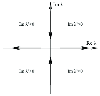
Figure 1: The oriented integration contour $\Gamma$ and regions of analiticity of $a(\lambda)$ (the first and third quadrants) and $\tilde{a}(\lambda)$ (the second and fourth quadrants) respectively.

$$a(\lambda)=\prod_{j=1}^{N}\frac{\lambda^{2}-\lambda_{j}^{2}}{\lambda^{2}-\lambda_{j}^{\ast 2}}\exp\left\{i\theta+\frac{1}{2\pi i}\right.$$

$$\left.\times\int_{\Gamma}\frac{\mu\ln(1+\sigma\,\mathrm{sgn}\,\mu^{2}|\,b(\mu)|^{\,2})}{\mu^{2}-\lambda^{2}}\,d\mu\right\}.$$ (33)

From Eqs. (19) and (21) we have $a(0)=1$, then, setting $\lambda=0$ in Eq. (33), one can find $\theta$ in terms of the scattering data

$$\theta=-4\sum_{j=1}^{N}\arg\lambda_{j}+\frac{1}{2\pi}\int_{\Gamma}\frac{\ln(1+\sigma\,\mathrm{sgn}\,\mu^{2}|\,b(\mu)|^{2})}{\mu}d\mu,$$ (34)

where $\arg\lambda_{j}=\gamma_{j}/2$ for $\sigma=-1$ and $\arg\lambda_{j}=\pi/2-\gamma_{j}/2$ for $\sigma=1$. From Eqs. (33) and (34) we have

$$a(\lambda)=\prod_{j=1}^{N}\frac{\lambda_{j}^{\ast 2}}{\lambda_{j}^{2}}\frac{(\lambda^{2}-\lambda_{j}^{2})}{(\lambda^{2}-\lambda_{j}^{\ast 2})}\exp\left\{\frac{1}{2\pi i}\right.$$

$$\left.\times\int_{\Gamma}\frac{\lambda^{2}\ln(1+\sigma\,\mathrm{sgn}\,\mu^{2}|\,b(\mu)|^{\,2})}{\mu(\mu^{2}-\lambda^{2})}\,d\mu\right\}.$$ (35)

The time evolution of the scattering data can be found, in a standard way Zakharov_book , from Eq. (9) by considering the limit $x\rightarrow\pm\infty$. Then

$$\lambda_{j}(t)=\lambda_{j}(0),$$ (36)

$$b_{j}(t)=b_{j}(0)\exp[-i/(2\lambda^{2}_{j})t],$$ (37)

$$b(\lambda,t)=b(\lambda,0)\exp[-i/(2\lambda^{2})t],$$ (38)

and in the following we denote $\lambda_{j}(0)\equiv\lambda_{j}$, $b_{j}(0)\equiv b_{j}$ and $b(\lambda,0)\equiv b(\lambda)$.

$$a(\lambda)=\prod_{j=1}^{N}\frac{\lambda_{j}^{\ast 2}}{\lambda_{j}^{2}}\frac{(\lambda^{2}-\lambda_{j}^{2})}{(\lambda^{2}-\lambda_{j}^{\ast 2})}$$ (39)

Since $S(\lambda)$ is diagonal in this case, it can be factorized in such a way $S^{\,-}(\lambda)=S^{\,+}(\lambda)S(\lambda)$, that the Jost solution matrices $M^{\,\pm}$ is expressed through a common matrix $A(x,t,\lambda)$

$$M^{\,\pm}(x,t,\lambda)=A(x,t,\lambda)S^{\,\pm}(\lambda),$$ (40)

where

$$S^{\,+}=\mathrm{diag}\,\left(\prod_{j=1}^{N}\frac{\lambda_{j}}{\lambda_{j}^{\ast}(\lambda^{2}-\lambda_{j}^{2})},\prod_{j=1}^{N}\frac{\lambda_{j}^{\ast}}{\lambda_{j}(\lambda^{2}-\lambda_{j}^{\ast 2})}\right)$$ (41)

and $S^{\,-}=\sigma_{1}S^{\,+}\sigma_{1}$. Since $A(\lambda)$ is analytical in the $\lambda$ plane, it follows from Eqs. (22)-(25) and (40) that diagonal and off-diagonal elements of the matrix $A(\lambda)E^{-1}(\lambda)$ are polynomials in $\lambda$ of degrees $2N$ and $2N-1$ respectively, and one can write

$$A(x,t,\lambda)=\begin{pmatrix}A_{11}^{(0)}&0\\ 0&A_{22}^{(0)}\end{pmatrix}\exp(-i\lambda^{2}\sigma_{3}x)$$

$$+\sum_{k=1}^{N}\lambda^{2k-1}\begin{pmatrix}\lambda A_{11}^{(k)}&A_{12}^{(k)}\\ A_{21}^{(k)}&\lambda A_{22}^{(k)}\end{pmatrix}\exp(-i\lambda^{2}\sigma_{3}x),$$ (42)

where $A^{(k)}_{mn}$ with $k=0\dots N$ and $m,n=1,2$ are still unknown functions. Setting here $\lambda=0$, we readily get from Eqs. (21) and (40) the expressions for the functions $A_{11}^{(0)}(x,t)$ and $A_{22}^{(0)}(x,t)$

$$A_{11}^{(0)}=A_{22}^{(0)}=-\prod_{k=1}^{N}|\lambda_{k}|^{2}.$$ (43)

From (32) and the fact $S^{\pm}=S^{\mp}$, it follows that the columns of $A(x,t,\lambda)$ satisfy the relations

$$A_{1}(x,t,\lambda_{j})=b_{j}(t)A_{2}(x,t,\lambda_{j}),$$ (44)

$$A_{2}(x,t,\lambda_{j}^{\ast})=\sigma b_{j}^{\ast}(t)A_{1}(x,t,\lambda_{j}^{\ast}).$$ (45)

Substituting Eqs. (42) and (43) into Eqs. (44) and (45), one can obtain the linear system of equations for the functions $A_{11}^{(k)}(x,t)$ and $A_{12}^{(k)}(x,t)$

$$\sum_{k=1}^{N}\lambda_{j}^{2k}A_{11}^{(k)}-\sum_{k=1}^{N}\lambda_{j}^{2k-1}\,\,c_{j}A_{12}^{(k)}=\prod_{k=1}^{N}|\lambda_{k}|^{2},$$ (46)

$$\sum_{k=1}^{N}\lambda_{j}^{\ast 2k}A_{11}^{(k)}-\sum_{k=1}^{N}\lambda_{j}^{\ast 2k-1}\,\,\sigma c_{j}^{\ast-1}A_{12}^{(k)}=\prod_{k=1}^{N}|\lambda_{k}|^{2},$$ (47)

where

$$c_{j}=b_{j}\exp\left(2i\lambda_{j}^{2}x-i/(2\lambda^{2}_{j})t\right).$$ (48)

The remaining functions $A_{21}^{(k)}(x,t)$ and $A_{22}^{(k)}(x,t)$ can be found from the symmetry properties Eq. (16)

$$A_{22}^{(k)}(x,t)=A_{11}^{(k)\ast}(x,t),\quad A_{21}^{(k)}(x,t)=\sigma A_{12}^{(k)\ast}(x,t).$$ (49)

Equations (40) and (42) determine the $N$-soliton Jost solutions. By direct substitution one can check that Eq. (42) is compatible with Eqs. (6), (7) and (40) if and only if

$$u_{x}=2iA_{12}^{(N)}/A_{22}^{(N)}.$$ (50)

Equation (50) can also be obtained from Eqs. (27) and (40). Although in the case $N=1$ the integration for obtaining $u$ can be performed explicitly, it is practically impossible already for $N\geqslant 2$. However, using the dressing method, Lennels Lenells2010_N-soliton obtained an explicit formula for the $N$-soliton solution of Eq. (2) (later on, an analogues formula was obtained by Matsuno Matsuno_bright2012 by using the Hirota bilinearization method) which in our notations (if $\sigma=-1$) has the form

$$u(x,t)=\sum_{k,j=1}^{N}c_{k}^{\ast}(K^{-1})_{kj},$$ (51)

where the elements of the $N\times N$ matrix $K$ are

$$K_{jk}=\frac{\lambda_{j}\lambda_{k}^{\ast}}{\lambda_{k}^{\ast 2}-\lambda_{j}^{2}}(\lambda_{j}+\lambda_{k}^{\ast}c_{j}c_{k}^{\ast}).$$ (52)

The case $N=1$ corresponds to the one-soliton solution and from Eqs. (51) and (52) one can readily get

$$u=\frac{(\lambda_{1}^{\ast 2}-\lambda^{2}_{1})c^{\ast}_{1}}{|\lambda_{1}|^{2}\left(\lambda_{1}+\lambda_{1}^{\ast}|c_{1}|^{2}\right)}$$ (53)

On the other hand, from Eqs. (47) and (50) we have ($\sigma=-1$)

$$u_{x}=2i(\lambda_{1}^{2}-\lambda_{1}^{\ast 2})\frac{(\lambda_{1}^{\ast}+\lambda_{1}|c_{1}|^{2})c_{1}^{\ast}}{(\lambda_{1}+\lambda_{1}^{\ast}|c_{1}|^{2})^{2}}.$$ (54)

Next, we parametrize the complex numbers $\lambda_{1}$ and $b_{1}$ in terms of four real parameters $\Delta>0$, $0<\gamma<\pi$, $x_{0}$ (the initial position of the soliton) and $\phi_{0}$ (the initial phase) as

$$\lambda_{1}^{2}=\Delta^{2}(\cos\gamma+i\sin\gamma),$$ (55)

$$b_{1}=\exp(2\Delta^{2}x_{0}\sin\gamma+i\phi_{0}).$$ (56)

Then the one-soliton solution Eq. (53) takes the form

$$u=\frac{\sin\gamma\exp(-i\Phi)}{i\Delta\cosh(z+i\gamma/2)},$$ (57)

where

$$z=2\Delta^{2}\left(x-x_{0}+\frac{t}{4\Delta^{4}}\right)\sin\gamma,$$ (58)

and

$$\Phi=2\Delta^{2}\left(x-\frac{t}{4\Delta^{4}}\right)\cos\gamma+\phi_{0}.$$ (59)

From Eqs. (54), (55) and (56) we have

$$u_{x}=-\frac{2\Delta\sin\gamma\cosh(z-i\gamma/2)\exp(-i\Phi)}{\cosh^{2}(z+i\gamma/2)}.$$ (60)

After integration in Eq. (60) we recovered Eq. (57). Under this, $c_{1}=\exp(-z+i\Phi)$. An explicit expression for $u$ in terms of the soliton amplitude and phase is

$$u=\frac{\sin\gamma\exp\{-i\Phi-i\arctan[\tanh z\tan(\gamma/2)]\}}{i\Delta\sqrt{\cosh^{2}z-\sin^{2}(\gamma/2)}}.$$ (61)

Earlier this solution was obtained by Davydova and Lashkin Lashkin1991 ; Lashkin1994 without using the IST. The soliton velocity $v$, amplitude $A$ and the characteristic halfwidth of the soliton $w$ are

$$v=-\frac{1}{4\Delta^{4}},\quad A=\frac{\sin\gamma}{\Delta},\quad w=\frac{1}{2\Delta^{2}\sin\gamma}.$$ (62)

It is seen that the soliton can not be motionless, and it moves only in the negative direction of $x$-axis. Equation (1) admits also rational $N$-soliton solutions, i.e. solitons with algebraic decay at infinity. These solutions arise from the solitons with exponential decay in the limit $\gamma_{j}\rightarrow\pi$. In the case $N=1$, from (57) one can obtain

$$u=\frac{2\exp(-i\Phi)}{i\Delta-4\Delta^{3}y},$$ (63)

where $y=x-x_{0}+t/(4\Delta^{4})$. This algebraic soliton of Eq. (1) was first obtained in Ref. Lashkin1994 and then rediscovered in Ref. Lenells2009_Nonlinearity . In terms of the amplitude and phase, Eq. (63) takes the form

$$u=\frac{2\exp[-i\Phi+i\,\mathrm{arccot}\,(4\Delta^{2}y)]}{\Delta\sqrt{1+16\Delta^{4}y^{2}}}.$$ (64)

Taking the Fourier transform in Eq. (57),

$$u(\omega,q)=\int_{-\infty}^{\infty}u(x,t)\exp(-i\omega t+iqx)\,dx,$$ (65)

one can find the one-soliton field in the spectral space as

$$u(\omega,q)=\frac{2\pi A\exp(-\gamma\varkappa/2+i\psi_{0})}{i\cosh(\pi\varkappa/2)}\delta\left(\omega-qv-\frac{\cos\gamma}{\Delta^{2}}\right),$$ (66)

where $\delta(x)$ is the Dirac delta function, and

$$\varkappa=\cot\gamma-\frac{q}{k_{0}},\quad k_{0}=\frac{1}{w},\quad\psi_{0}=\phi_{0}-k_{0}x_{0}.$$ (67)

The presence of the $\delta$-function reflects the fact that a single soliton is a stationary structure, i. e. it moves with the constant velocity $v$, and the term $\cos\gamma/\Delta^{2}$ corresponds to the nonlinear frequency shift. Thus, as is seen from Eqs. (65) and (66), the soliton can be treated as a localized wavepacket of monochromatic waves with self-consistent amplitudes and phases.

Following Ref. Gerdzhikov80 , and using the fact that the $x$-part of the Lax pair Eq. (6) is simply related to the $x$-part of the Lax pair of the DNLS equation by the replacement $u\rightarrow u_{x}$, one can write $u_{x}(x,t)$ in terms of the scattering data and squared eigenfunctions of Eq. (6) as

$$u_{x}(x,t)=-4i\sum_{j=1}^{N}(C_{j}\psi_{1,j}^{2}+C_{j}^{\ast}\tilde{\psi}_{1,j}^{2})-\frac{1}{\pi}\int_{\Gamma}(r\psi_{1}^{2}+\tilde{r}\tilde{\psi}_{1}^{2})\,d\lambda,$$ (68)

where $r(\lambda)=b(\lambda)/a(\lambda)$ is the reflection coefficient, $\tilde{r}(\lambda)=\tilde{b}(\lambda)/\tilde{a}(\lambda)=r^{\ast}(\lambda^{\ast})$, $C_{j}=b_{j}/\dot{a}_{j}$ with $\dot{a}_{j}=da/d\lambda|_{\lambda=\lambda_{j}}$. Here, the contribution of the discrete spectrum ($\sum_{j=1}^{N}$) is explicitly separated from that of the continuous one ($\int\,d\lambda$). The first term in Eq. (68) is the soliton contribution, while the second one corresponds to the radiative part of the field. In the asymptotic $t\rightarrow\infty$, a generic initial field $u_{x}(x,0)$ will reshape itself into a set of $N$ solitons (if any) and continuous radiation (quasilinear waves). The latter always disperses away and decays, while the solitons will propagate as coherent units. In the linear limit, Eq. (1) describes the linear waves with the dispersion relation $\omega=1/k$ (taking $u(x,t)\sim\exp(i\omega t-ikx)$) that corresponds to the short-wavelength ion-cyclotron (ion Bernstein) waves in a plasma Trievel86 ; Akhiezer (see A). On the other hand, from Eq. (20) in the linear limit we have $\psi_{1}\rightarrow 0$ and $\tilde{\psi}_{1}\rightarrow\exp(-i\lambda^{2}x)$ (note that this situation takes place as well for the NLS equation Bullough1980 ) so that ($t$-dependence remains the same as before) the function $\tilde{\psi}_{1}^{2}$ simply reduces to $\exp[-2i\lambda^{2}x+it/(2\lambda^{2})]$ and $\tilde{r}(\lambda)$ is just the linear Fourier transform of $u_{x}(x,t)$. This reflects the general property of the IST (see, for example, Ref. Bullough1980 ): in the linear limit it is equivalent to the usual Fourier method. Then, considering the radiative component as a superposition of free waves governed by the linearized Eq. (1), one can conclude that the spectral parameter $\lambda$ is connected to the wave number of the emitted quasilinear waves $k$ by the relation

$$k=2\lambda^{2},$$ (69)

where $\lambda^{2}$ is real. Under this, the second term in Eq. (68) that corresponds to the radiative part of the field $u_{x,\,rad}$ can be written as

$$u_{x,\,rad}(x,t)=-\frac{1}{\pi}\int_{-\infty}^{\infty}[r(k)\psi_{1}^{2}(k)+\tilde{r}(k)\tilde{\psi}_{1}^{2}(k)]\,dk.$$ (70)

III Hamiltonian structure and Integrals of motion

In Refs. Lenells2009_Nonlinearity ; Lenells2009_derivation it was shown that Eq. (1) arises from the first negative flow of the Kaup–-Newell hierarchy of the DNLS equation Kaup1978

$$\begin{pmatrix}u_{x}\\ \sigma u_{x}^{\ast}\end{pmatrix}_{t}=\sigma_{1}\frac{\partial}{\partial x}\,\mathrm{grad}\,H_{n-1}=J_{2}\,\mathrm{grad}\,H_{n},$$ (71)

where $\mathrm{grad}\equiv(\delta/\delta u,\sigma\,\delta/\delta u_{x}^{\ast})^{\mathrm{T}}$, the superscript $\mathrm{T}$ denotes transposition, and the operator $J_{2}$ are determined by

$$J_{2}=\begin{pmatrix}-uu_{x}&i+\sigma u_{x}u^{\ast}\\ -i+\sigma uu_{x}^{\ast}&-u^{\ast}u_{x}^{\ast}\end{pmatrix}.$$ (72)

Then, the infinite sequence of conservation laws $H_{n}$ are constructed recursively from the relation

$$\mathrm{grad}\,H_{n+1}=J_{2}^{-1}\sigma_{1}\frac{\partial}{\partial x}\,\mathrm{grad}\,H_{n}.$$ (73)

where the inverse of $J_{2}$ is given by

$$J_{2}^{-1}=\begin{pmatrix}u^{\ast}u_{x}^{\ast}&i+\sigma uu_{x}^{\ast}\\ -i+\sigma u_{x}u^{\ast}&uu_{x}\end{pmatrix}.$$ (74)

Gerdzhikov et. al. showed Gerdzhikov80 that the DNLS equation is completely integrable Hamiltonian system, and calculated the corresponding action-angle variables (see also Ref. Sasaki1982 ). They obtained also the local and nonlocal conservation laws in terms of the spectral data. Following Ref. Gerdzhikov80 , and using the simple relation between Eq. (6) and the $x$-part of the Lax pair of the DNLS equation, one can obtain an explicit expression for the local and nonlocal conservation laws $I_{n}$ of Eq. (1) in the form

$$I_{n}=\frac{1}{4|n|}\left\{i\int_{-\infty}^{\infty}(\sigma u_{x}^{\ast},u_{x})\hat{K}^{n}\begin{pmatrix}u_{x}\\ \sigma u_{x}^{\ast}\end{pmatrix}\,dx\right.$$

$$\left.+4\int_{-\infty}^{\infty}\int_{x}^{\infty}(\sigma u_{y}^{\ast},-u_{y})\hat{K}^{n+1}\begin{pmatrix}u_{y}\\ \sigma u_{y}^{\ast}\end{pmatrix}\,dy\,dx\right\},$$ (75)

where the operator $\hat{K}$ is determined by

$$\hat{K}=\frac{i}{2}\left[1+i\begin{pmatrix}u_{x}\\ \sigma u_{x}^{\ast}\end{pmatrix}(\sigma u_{x}^{\ast},-u_{x})\right]\sigma_{3}\frac{\partial}{\partial x}.$$ (76)

Under this, the functionals $I_{n}$ are the expansion coefficients in $\ln a(\lambda)$

$$\ln a(\lambda)=i\theta+\sum_{n=1}^{\infty}\frac{I_{n}}{\lambda^{2n}}=\sum_{n=0}^{\infty}I_{-n}\lambda^{2n},$$ (77)

and from Eq. (33) one can get the so-called trace formulae

$$I_{n}=-\frac{1}{|n|}\sum_{j=1}^{N}\left(\lambda_{j}^{2n}-\lambda_{j}^{\ast 2n}\right)$$

$$+\frac{i\,\mathrm{sgn}\,n}{2\pi}\int_{\Gamma}\mu^{2n-1}\ln(1+\sigma\,\mathrm{sgn}\,\mu^{2}|\,b(\mu)|^{2})\,d\mu.$$ (78)

From the physical point of view, the quantities $u$ and $-u_{x}$ correspond to the electric potential and electrical field respectively Lashkin1991 ; Lashkin1994 (see Appendix A).Then, the electrical energy $E$ and the momentum $P$ are

$$E=2\sigma\theta=\int_{-\infty}^{\infty}|u_{x}|^{2}\,dx,$$ (79)

$$P=iI_{-1}=\frac{i}{2}\int_{-\infty}^{\infty}(u^{\ast}u_{x}-uu_{x}^{\ast})\,dx.$$ (80)

The energy and momentum can be explicitly expressed in terms of the discrete (solitonic) and continuous (radiative) scattering data. The expression for the energy Eq. (79) follows from Eq. (34) where, for definiteness, we take $\sigma=-1$,

$$E=4\sum_{j=1}^{N}\gamma_{j}-\frac{1}{\pi}\int_{\Gamma}\frac{\ln(1-\mathrm{sgn}\,\lambda^{2}|\,b(\lambda)|^{2})}{\lambda}\,d\lambda.$$ (81)

The expression for the momentum $P$ follows from Eqs. (78) and (80) and has the form

$$P=2\sum_{j=1}^{N}\frac{\sin\gamma_{j}}{\Delta_{j}^{2}}-\frac{1}{2\pi}\int_{\Gamma}\frac{\ln(1-\mathrm{sgn}\,\lambda^{2}|\,b(\lambda)|^{2})}{\lambda^{3}}\,d\lambda.$$ (82)

Using the relation Eq. (69) between the spectral parameter $\lambda$ and the wave number $k$ of the emitted quasilinear waves, one can also write for the energy and the momentum

$$E=4\sum_{j=1}^{N}\gamma_{j}+\int_{-\infty}^{\infty}\mathcal{E}_{rad}(k)\,dk,$$ (83)

and

$$P=4\sum_{j=1}^{N}\gamma_{j}+\int_{-\infty}^{\infty}\mathcal{P}_{rad}(k)\,dk,$$ (84)

where $\mathcal{E}_{rad}(k)$ and $\mathcal{P}_{rad}(k)$ are the spectral energy and momentum densities (in the wave number domain) carried by radiation respectively , determined by

$$\mathcal{E}_{rad}(k)=-\frac{\ln(1-\mathrm{sgn}\,k|\,b(k)|^{2})}{2\pi k},\quad\mathcal{P}_{rad}(k)=\frac{\mathcal{E}_{rad}(k)}{k}.$$ (85)

For a single soliton Eq. (61) one can express the energy and the momentum through the soliton velocity $v$ and the amplitude $A$ as

$$E=4\arcsin[(4|v|)^{-1/4}A]+\int_{-\infty}^{\infty}\mathcal{E}_{rad}(k)\,dk,$$ (86)

and

$$P=2(4|v|)^{1/4}A+\int_{-\infty}^{\infty}\mathcal{P}_{rad}(k)\,dk.$$ (87)

IV Dynamics of the scattering data in the presence of perturbations

Equation (3) can be cast in the matrix form

$$\partial_{t}U-\partial_{x}V+[U,V]=P,$$ (88)

where

$$P=\begin{pmatrix}0&\lambda p\\ \sigma\lambda p^{\ast}&0\end{pmatrix}.$$ (89)

From Eq. (88) and the fact that $M^{\pm}$ satisfies Eq. (6) one can get

$$(\partial_{x}-U)(\partial_{t}-V)M^{\pm}=PM^{\pm}.$$ (90)

Introducing a new unknown $J^{\pm}(x,t,\lambda)$ defined through the relation

$$(\partial_{t}-V)M^{\pm}=M^{\pm}J^{\pm},$$ (91)

and substitute Eq. (91) in Eq. (90) one can see that $J^{\pm}$ should satisfy the equation $\partial_{x}J^{\pm}=M^{\pm\,-1}PM^{\pm}$, and, therefore, by integrating we get $J^{\pm}=C^{\,\pm}+\int_{\pm\infty}^{x}M^{\pm\,-1}PM^{\pm}dx^{\prime}$, where the constant matrices $C^{\,\pm}$ are determined from the boundary conditions at $x\rightarrow\pm\infty$. Since $V=i/(4\lambda^{2})\sigma_{3}$ as $x\rightarrow\pm\infty$, we have from Eq. (91) $C^{\pm}=-i/(4\lambda^{2})\sigma_{3}$, and, hence, the following equations of motion for $M^{\pm}$

$$(\partial_{t}-V)M^{\pm}=M^{\pm}\left[-\frac{i}{4\lambda^{2}}\sigma_{3}+\int_{\pm\infty}^{x}(M^{\pm})^{-1}PM^{\pm}dx^{\prime}\right].$$ (92)

Equation (92) is valid only for $\mathrm{Im}\,\lambda^{2}=0$. Introducing the matrix $M(x,t,\lambda)=(M_{1}^{-},M_{2}^{+})$, columns of which admit analytical continuation to $\mathrm{Im}\,\lambda^{2}>0$, and defining the matrix $J(x,t,\lambda)=(J_{1}^{-},J_{2}^{+})$ we get

$$(\partial_{t}-V)M=MJ,$$ (93)

one can similarly obtain

$$J_{1}=\begin{pmatrix}-\dfrac{i}{4\lambda^{2}}\\ 0\end{pmatrix}+\int_{-\infty}^{x}M^{-1}P\varphi dx^{\prime},$$ (94)

$$J_{2}=\begin{pmatrix}0\\ \dfrac{i}{4\lambda^{2}}\end{pmatrix}-\int_{x}^{\infty}M^{-1}P\psi dx^{\prime}.$$ (95)

Thus, we have the equations of motion valid for $\mathrm{Im\,\lambda^{2}>0}$ except at $\lambda_{j}$, where $M$ fails to be invertible. Making the assumption that the zeros $\lambda=\lambda_{j}$ are simple, one can show (see below), that each singularity is removable since $\det M=a(\lambda)$. Differentiating Eq. (12) with respect to $t$, and using Eq. (92) yields

$$\partial_{t}S(t,\lambda)-\frac{i}{4\lambda^{2}}[\sigma_{3},S(t,\lambda)]$$

$$=\int_{-\infty}^{\infty}(M^{+})^{-1}(x,t,\lambda)PM^{-}(x,t,\lambda)dx.$$ (96)

The equations of motion for the coefficients $a(t,\lambda)$ and $b(t,\lambda)$ are contained in Eq. (96):

$$\frac{\partial a}{\partial t}=\lambda\int_{-\infty}^{\infty}(p\psi_{2}\varphi_{2}-\sigma p^{\ast}\psi_{1}\varphi_{1})\,dx,$$ (97)

$$\frac{\partial b}{\partial t}+\frac{i}{2\lambda^{2}}b=-\lambda\int_{-\infty}^{\infty}(p\tilde{\psi_{2}}\varphi_{2}-\sigma p^{\ast}\tilde{\psi_{1}}\varphi_{1})\,dx.$$ (98)

The expression defining the zeros $\lambda_{j}(t)$ of $a(t,\lambda)$ is $a(t,\lambda_{j}(t))=0$. Differentiating with respect to $t$ gives

$$\partial_{t}a(t,\lambda_{j}(t))+\frac{\partial\lambda_{j}}{\partial t}\,\dot{a}_{j}=0,$$ (99)

where $\dot{a}_{j}=da/d\lambda|_{\lambda=\lambda_{j}}$. Using (97) and (99) we have

$$\frac{\partial\lambda_{j}^{2}}{\partial t}=-\frac{2\lambda_{j}^{2}}{\dot{a}_{j}}\int_{-\infty}^{\infty}(p\psi_{2,j}\varphi_{2,j}-\sigma p^{\ast}\psi_{1,j}\varphi_{1,j})\,dx,$$ (100)

where $\psi_{2,j}$, $\varphi_{2,j}$, $\psi_{1,j}$, and $\varphi_{1,j}$ are the corresponding Jost solutions evaluated at $\lambda=\lambda_{j}$. To obtain evolution equation for $b_{j}$, we differentiate Eq. (32) with respect to $t$, use Eqs. (93), (94) and (95), and take the limit $\lambda\rightarrow\lambda_{j}$ applying (since $\det M(\lambda_{j})=a(\lambda_{j})=0$) the l’Hopitale rule and using again Eq. (32). As a result, one obtains

$$\frac{\partial b_{j}}{\partial t}+\frac{i}{2\lambda_{j}^{2}}b_{j}=\frac{\lambda_{j}}{\dot{a}_{j}}\int_{-\infty}^{\infty}\left\{p\,\varphi_{2}\frac{\partial}{\partial\lambda}\left(\varphi_{2}-b_{j}\psi_{2}\right)\right.$$

$$\left.-\sigma p^{\ast}\,\varphi_{1}\frac{\partial}{\partial\lambda}\left(\varphi_{1}-b_{j}\psi_{1}\right)\right\}dx^{\prime},$$ (101)

where, after differentiating, the integrand is evaluated at $\lambda=\lambda_{j}$. Equations (97), (98), (100) and (101) describe the evolution of the scattering data.

If $p[u,u^{\ast}]$ is a small perturbation, one can substitute the unperturbed $N$-soliton solutions $\psi$, $\tilde{\psi}$, $\varphi$ and $\tilde{\varphi}$ into the right-hand side of Eqs. (97), (98), (100) and (101). This yields evolution equations for the scattering data in the lowest approximation of perturbation theory. This procedure can be iterated to yield higher orders of perturbation theory. The appearing hierarchy of equations are applied to arbitrary number of solitons and, in particular, describe nontrivial many-soliton effects in the presence of perturbations.

V Perturbations in the DLFL equation

In reality, as mentioned above, the DLFL equation describing nonlinear ion-cyclotron waves in a collisionless plasma may contain additional terms which in some cases are treated as small perturbations. Below we give a summary of some of the physical mechanisms that are often encountered in applications to plasma physics, and write out the corresponding terms of the perturbation $p$, where $\epsilon$ is a real constant depending on the specific model. In particular, these are (the first two will be further explored in detail in this section):

• Linear damping in collisionless plasma, see Eq. (112).

• Multiplicative noise, see Eqs. (132) and (133).

• Linear damping in collisional plasma Rukhadze84 ; Volland1984 ,

  $$p=\epsilon u_{xxx},$$ (102)

  where the perturbation has a diffusive character, and $\epsilon$ depends on the plasma ion viscosity and/or resistivity. This type of perturbation is important in weakly ionized plasmas, in particular, in the plasma of Earth’s ionosphere Volland1984 .

• Nonlinear Landau damping Ichikawa1973 ; Scorich2010 ,

  $$p=\epsilon u_{x}\,\mathcal{P}\int_{-\infty}^{\infty}\frac{|u(x^{\prime},t)|^{2}}{x^{\prime}-x}dx^{\prime},$$ (103)

  where $\mathcal{P}$ is the principal value of the integral. The non-local perturbation term $p$ represents the effect of resonant particles on the wave modulations. The coefficient $\epsilon$ depends on the velocity distributions of the particle species.

• External pump used in the method of plasma heating in the ion cyclotron range of frequency in plasma magnetic confinement devices Rukhadze84 ; Adam1987 ,

  $$p=\epsilon\exp(i\omega_{0}t),$$ (104)

  where the pump frequency $\omega_{0}$ is usually close to the ion-cyclotron frequency.

• Density or/and temperature gradient (or arbitrary inhomogeneity), and also curvature of the external magnetic field Petviashvili_book ; Rukhadze84 ; Adam1987 ,

  $$p=\epsilon F(x)u_{x},$$ (105)

  where $F(x)$ is often a linear function of $x$.

• Weak interaction with the low-frequency magnetosonic wave Petviashvili_book ,

  $$p=\epsilon bu_{x},$$ (106)

  with

  $$b_{tt}-\chi b_{xx}=(|u|^{2})_{xx},$$ (107)

  where $b$ is the perturbation of magnetic field associated with the magnetosonic wave, and $\chi$ is the dimensionless Alfvén speed.

In this section we study the effect of the perturbing term in the right-hand side of Eq. (3) on a single soliton ($N=1$) described by Eq. (57) and take $\sigma=-1$. Two different cases will be considered: (i) a linear damping and (ii) an external multiplicative noise. From the physical point of view, the first one corresponds to collisionless Landau damping. The second case corresponds to fluctuations of an external magnetic field or the influence of a turbulent environment.

Note, that in the first case, the damping is irreversible and the energy (both the soliton and the radiative parts) disappears in such a system. In the second case, the perturbation has conservative character and the total energy is conserved.

For the case $N=1$, the evolution equation for the discrete scattering data $\lambda_{1}$ follows from Eq. (100),

$$\frac{\partial\lambda_{1}^{2}}{\partial t}=-\frac{2\lambda_{1}^{2}}{\dot{a}_{1}}\int_{-\infty}^{\infty}(p\psi_{2,1}\varphi_{2,1}+p^{\ast}\psi_{1,1}\varphi_{1,1})dx,$$ (108)

where the unperturbed one-soliton Jost functions $\varphi_{1,1}$,$\varphi_{2,1}$,$\psi_{1,1}$ and $\psi_{1,1}$ are determined by Eqs. (168)-(171). After calculating $\dot{a}_{1}$ from Eq. (161), using Eqs. (58) and (59), and making change of variables $z\rightarrow-z$ in the second term of the integrand in Eq. (108), this equation can be written in a simple form

$$\frac{\partial\lambda_{1}^{2}}{\partial t}=-i\lambda_{1}^{3}\int_{-\infty}^{\infty}\frac{\mathrm{e}^{z}}{\left(\lambda_{1}\mathrm{e}^{-z}+\lambda_{1}^{\ast}\mathrm{e}^{z}\right)^{2}}[R(z)+R^{\ast}(-z)]dz,$$ (109)

where $R(z)=p\exp(i\Phi)$. Taking into account Eqs. (13) and (14), the evolution equation Eq. (98) for the continuous scattering data $b(\lambda)$ can be rewritten as

$$\partial_{t}b+\frac{i}{2\lambda^{2}}b=-\frac{\lambda}{a(\lambda)}\int[p(\tilde{a}\varphi_{2}+b\tilde{\varphi}_{2})\varphi_{2}$$

$$+p^{\ast}(\tilde{a}\varphi_{1}+b\tilde{\varphi}_{1})\varphi_{1}]\,dx,$$ (110)

and has the form

$$\partial_{t}b+\frac{i}{2\lambda^{2}}b=-\frac{\lambda}{a(\lambda)}\int(p\varphi_{2}^{2}+p^{\ast}\varphi_{1}^{2})\,dx,$$ (111)

where we have used that $\varphi=a(\lambda)\tilde{\psi}$ for the unperturbed scattering data $a(\lambda)$ and soliton Jost functions $\varphi_{1,2}$ which are determined by Eqs. (161) and (162).

V.1 Linear damping

Linear damping of waves in a plasma occurs due to collisions or/and, in collisionless plasma, due to collisionless Landau damping. The first case is more typical for a weakly ionized plasma and the damping usually has the character of a diffusion-type dissipation with the damping rate $\Gamma_{k}=\mathrm{Im}\,\omega_{k}\sim k^{2}$, where $\omega_{k}$ is the frequency of plasma wave and $k$ is the wave number. The second case corresponds to a fully ionized plasma where collisionless damping dominates. In this paper, we restrict ourselves to the case of collisionless plasma. As is well known, the Landau damping rate $\Gamma_{k}$ for all types of plasma waves is not a polynomial in the wavenumber $k$ and is an integral operator in $x$-space Trievel86 ; Rukhadze84 , but in practical applications (for optimal wavenumbers) it can be estimated as independent of $k$ so that we use $\Gamma_{k}=\Gamma\ll\mathrm{Re}\,\omega_{k}$. In physical variables, the Landau damping rate $\Gamma$ for the considered short-wavelength ion-cyclotron waves can be found in Ref. Perkins1976 . Thus, the perturbation term in Eq. (3) can be written as

$$p=-\Gamma u_{x},$$ (112)

and treated as a small perturbation.

V.1.1 adiabatic approximation

Substituting Eq. (112) into Eq. (109) and integrating, one can get

$$\frac{\partial\lambda_{1}^{2}}{\partial t}=2\Gamma\lambda_{1}^{2}(1-i\gamma-\gamma\cot\gamma).$$ (113)

Separating the real and imaginary parts in Eq. (113) we get equations for $\Delta$ and $\gamma$

$$\frac{\partial\Delta}{\partial t}=\Gamma\Delta(1-\gamma\cot\gamma),$$ (114)

$$\frac{\partial\gamma}{\partial t}=-2\Gamma\gamma.$$ (115)

From the latter equation we have $\gamma=\gamma_{0}\exp(-2\Gamma t)$, where $\gamma_{0}$ is the initial value of $\gamma$ at the moment $t=0$. Note that from Eq. (3) and the perturbation in the form Eq. (112) one can obtain the exact relation

$$\frac{\partial\theta}{\partial t}=-2\Gamma\theta,$$ (116)

where $\theta$ is defined by Eq. (29) and is an integral of motion in the absence of perturbations. In the terms of the scattering data $\theta$ is determined by Eq. (34) and for the one-soliton solution Eq. (57) we have $\theta=2\gamma$ so that we have Eq. (115). Integrating Eq. (114) yields

$$\Delta=\Delta_{0}\exp\left(\Gamma t-\Gamma\int_{0}^{t}\gamma(t^{{}^{\prime}})\cot\gamma(t^{{}^{\prime}})dt^{{}^{\prime}}\right),$$ (117)

where $\Delta_{0}$ is an initial value of $\Delta$ at $t=0$, and after calculating the integral in Eq. (117) we find $\Delta=\Delta_{0}$. Thus, as is seen from Eq. (62) , the soliton amplitude exponentially decays but the soliton velocity remains constant. Note that for this type of perturbation, the same dependence of the soliton parameters takes place for the NLS equation Kaup1976 . We would like to stress once again that the equations in the adiabatic approximation can be obtained from the corresponding integrals of motion without using the IST method.

V.1.2 radiative effects

The adiabatic approximation implies that $b(\lambda)=0$ and an unperturbed instantaneous shape of the soliton is assumed. Now we consider the radiative effects which are described by the continuous spectrum scattering data $a(\lambda)$ and $b(\lambda)$. In the presence of a perturbation the soliton emits radiation. Indeed, as the soliton’s amplitude is decreasing, as we have seen, it is slowly loosing energy. The total energy exponentially decays and soliton part of this energy is being dissipated away, but part of it is transferred to the quasilinear waves, or in other words, leads to excitation of the continuous spectrum.

In the case when a perturbation has the form Eq. (112) one can simplify Eq. (111) by using the relation

$$(\varphi_{1}\varphi_{2})_{x}=\lambda u_{x}\varphi_{2}^{2}-\lambda u_{x}^{\ast}\varphi_{1}^{2},$$ (118)

which directly follows from Eqs. (6) and (8). Then, taking into account that $u_{x}\rightarrow 0$ as $x\rightarrow\pm\infty$, one can obtain

$$\partial_{t}b+i\omega(\lambda)b=\frac{2\Gamma\lambda}{a(\lambda)}\int u_{x}\varphi_{2}^{2}\,dx,$$ (119)

where $\omega(\lambda)=1/(2\lambda^{2})$. After substituting Eqs. (54) and (162) into Eq. (119) and calculating the integral in the right-hand side of Eq. (119), we find

$$\partial_{t}b+i\omega(\lambda)b=\Gamma\mathrm{e}^{i\beta(\lambda,\gamma)t}F(\lambda,\gamma)$$ (120)

where the functions $\beta(\lambda,\gamma)$ and $F(\lambda,\gamma)$ are defined by

$$\beta(\lambda,\gamma)=\frac{\lambda^{2}}{2\Delta^{4}}-\frac{\cos\gamma}{\Delta^{2}},$$ (121)

and

$$F(\lambda,\gamma)=\frac{2\pi\Delta\lambda^{3}\left(\mathrm{e}^{-\gamma\alpha/2}-\mathrm{e}^{\gamma\alpha/2}\lambda^{2}/\Delta^{2}\right)}{[(\lambda^{2}-\Delta^{2})^{2}+4\lambda^{2}\Delta^{2}\sin^{2}(\gamma/2)]\cosh(\pi\alpha/2)},$$ (122)

respectively, where $\alpha=\cot\gamma-\lambda^{2}/(\Delta^{2}\sin\gamma)$ and the time dependence of $\gamma$ is determined by Eq. (115). Integration of Eq. (120) with an initial condition $b(0)=0$ yields

$$b(t)=\Gamma\mathrm{e}^{-i\omega(\lambda)t}\int_{0}^{t}\mathrm{e}^{i\omega(\lambda)t^{{}^{\prime}}+i\beta(\lambda,\gamma)t^{{}^{\prime}}}F(\lambda,\gamma)\,dt^{{}^{\prime}}.$$ (123)

There are two characteristic times of linear processes in the model – the damping time $\sim 1/\Gamma$ of linear waves with the dispersion $\omega_{k}=1/k$, and the dispersive time $\sim 1/\omega_{k}$ at which the packet of linear waves spreads out due to dispersion. At times $t\ll 1/\Gamma$, i. e. when the soliton has not yet completely decayed, one may simply put $\beta(\lambda,\gamma)=\beta(\lambda,\gamma_{0})$ and $F(\lambda,\gamma)=F(\lambda,\gamma_{0})$. Then

$$b(t)=\frac{i\Gamma F(\lambda,\gamma_{0})}{[\omega(\lambda)+\beta(\lambda,\gamma_{0})]}\left(\mathrm{e}^{-i\omega(\lambda)t}-\mathrm{e}^{i\beta(\lambda,\gamma_{0})t}\right).$$ (124)

In what follows we use the relation Eq. (69) between the wave number of the emitted quasilinear waves $k$ and the spectral parameter $\lambda$ and introduce the inverse soliton halfwidth $k_{0}=1/w$ from Eq. (62). From Eq. (124) for $|b(t)|^{2}$ we have

$$|b(t)|^{2}=\frac{4\sin^{2}(\Omega_{k}t/2)}{\Omega_{k}^{2}}\Gamma^{2}|F(\mu,\gamma_{0})|^{2},$$ (125)

where the function $|F(\mu,\gamma_{0})|^{2}$ is defined by

$$|F(\mu,\gamma_{0})|^{2}=\frac{4\pi^{2}\mu^{3}\sin^{3}\gamma_{0}\left(\mathrm{e}^{-\gamma_{0}\alpha/2}-\mathrm{e}^{\gamma_{0}\alpha/2}\mu\sin\gamma_{0}\right)^{2}}{[(1-\mu\sin\gamma_{0})^{2}+4\mu\sin\gamma_{0}\sin^{2}(\gamma_{0}/2)]^{2}\cosh^{2}(\pi\alpha/2)},$$ (126)

with $\alpha=\cot\gamma_{0}-\mu$, where $\mu=k/k_{0}$ is the ratio of the soliton halfwidth to the wavelength of the emitted waves, and

$$\Omega_{k}=\omega_{k}-\omega^{NL}_{k},\quad\omega_{k}=\frac{1}{k^{2}},\quad\omega^{NL}_{k}=kv+\frac{\cos\gamma_{0}}{\Delta^{2}}.$$ (127)

The frequency $\Omega_{k}$ includes both the linear $\omega_{k}$ and nonlinear frequency shift $\omega^{NL}_{k}$ (see Eq. (66)).

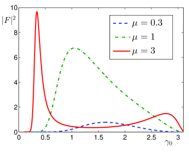
Figure 2: The function $|F(\mu,\gamma_{0})|^{2}$ for different $\mu=k/k_{0}$.

The function $|F(\mu,\gamma_{0})|^{2}$ as a function of $\gamma_{0}$ is plotted in Fig. 2 for different values $\mu$. At times $t\gg 1/\Omega_{k}$ but still $\Gamma t\ll 1$, one may consider an average over the period in Eq. (125) and put $\overline{\mathstrut\sin^{2}}=1/2$, where the overbar denotes the time average over the period. The emission intensity is characterized by its power, i.e. the energy emission rate. The absorbed emission power spectral density is

$$W_{rad}(k)=-\frac{d\mathcal{E}_{rad}(k)}{dt}=2\Gamma\mathcal{E}_{rad}(k).$$ (128)

If the perturbation is small enough then $|\,b(k)|\ll 1$ and from Eq. (85) we have

$$\mathcal{E}_{rad}(k)=\frac{|\,b(k)|^{2}}{2\pi|k|},$$ (129)

so that the absorbed emission power spectral density is

$$W_{rad}(k)=\frac{2\Gamma^{3}|F(\mu,\gamma_{0})|^{2}}{\pi|k|\Omega_{k}^{2}}.$$ (130)

In particular, for $\gamma_{0}=\pi/2$ that corresponds to the largest soliton amplitude for the fixed $\Delta$, we find

$$W_{rad}(\mu)=\frac{8\pi\Gamma^{3}k_{0}\mu^{4}\left(\mathrm{e}^{\pi\mu/4}-\mu\mathrm{e}^{-\pi\mu/4}\right)^{2}}{(1+\mu^{2})^{4}\cosh^{2}(\pi\mu/2)}.$$ (131)

The corresponding dependence is shown in Fig. 3

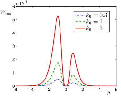
Figure 3: Spectral density of power emitted by the soliton v.s. $\mu=k/k_{0}$ for different $k_{0}$, $\Gamma=0.1$.

In coordinate space, the continuous spectrum appears as small oscillations (quasilinear waves) moving away from the soliton, where the wavelengths of these oscillations will be of the order of the width of the soliton ($\mu\sim 1$) as is seen from Fig. 3. As the soliton decays and its width increases, so does the typical wavelength of these oscillations. The width of the soliton is of order $1/k_{0}$, which is also the characteristic width $1/k$ of the emitted radiation.

At the end of this subsection, an important remark has to be made. It is well known Newell1978 ; Bullough1980 that the action of a perturbation in the form of linear damping (the effect of depth change) on a soliton of the KdV equation leads to the appearance of a long shelf containing as much mass as the original soliton. Under this, the total motion is not adiabatic, for although the soliton amplitude and the height the shelf itself are slowly varying quantities, the range of the shelf is not. Thus, the contribution of the continuous spectrum gives rise to a qualitatively new effect. Kaup and Newell Newell1978 noted that the presence of the shelf is connected with a singularity of the reflection coefficient in the framework of the IST and then correctly calculated the contribution corresponding to the continuous spectrum (the shelf). The singularity of the reflection coefficient on the real axis and, as a consequence, the emergence of the shelf in the presence of a perturbation also takes place for the dark soliton of the defocusing NLS equation Lashkin_dark2004 . Note that the shelf of the dark soliton of the defocusing NLS equation was studied in detail in Ref. Ablowitz_dark2011 using the so-called direct method. In our case of an exponentially localized soliton Eq. (57), one can see that a singularity in the reflection coefficient $r(k)=b(k)/a(k)$ does not arise (just like for the bright soliton of the focusing NLS equation) and the adiabatic approximation is valid, but the singularity appears for the algebraic soliton Eq. (63) since $\gamma\rightarrow\pi$. Then the adiabatic approximation is inapplicable and one can expect the emergence of a shelf.

V.2 Multiplicative noise

We now consider the perturbation in the form of a random multiplicative noise. In the presence of fluctuations of the magnetic field one can represent (for a given realization) the magnetic field Eq. (159) as $|u|^{2}\rightarrow|u|^{2}+\varepsilon$, where $\varepsilon$ stands for the random part of the field. Under this, the perturbation term in Eq. (3) takes the form

$$p=-i\varepsilon(x,t)u_{x},$$ (132)

where $\varepsilon(x,t)$ is assumed to be real gaussian homogeneous random field with the zero average $\langle\varepsilon\rangle=0$ and the correlator

$$\langle\varepsilon(x,t)\varepsilon(x^{\prime},t^{\prime})\rangle=D(x-x^{\prime})B(t-t^{\prime}),$$ (133)

where the angular brackets denote ensemble averaging.

Here we would like to make an important remark. If the function $\varepsilon(x,t)$ in Eq. (132) is independent of $x$, then the DLFL equation (3) with this kind of perturbation $p$ turns out to be (somewhat unexpectedly) completely integrable Kundu2010 . In this case, as can be easily verified, in the Eq. (9) for $V$ it is sufficient to make the substitution $i/(4\lambda^{2})\rightarrow i/(4\lambda^{2})-i\varepsilon(t)/2$ and the compatibility condition Eq. (5) still holds. In such a situation, of course, the term in the right-hand side of Eq. (3) is not a perturbation. In the NLS, DNLS, DLFL equations and some others with some specific additional terms, one speaks of "integrable perturbations" KunduTMF ). Below we consider only the case with the $x$-dependence in $\varepsilon(x,t)$.

Note that there is an important difference between the perturbations Eq. (112) and Eq. (132). In the case of a dissipative perturbation Eq. (112), the total energy vanishes over time, while for the perturbation Eq. (132), as can be easily shown, energy is conserved. Accordingly, for the dissipative perturbation we considered the initial problem at time $t=0$. For a conservative perturbation, we will focus on the stationary regime and assume that the perturbation, which is absent at infinity $t=-\infty$, turns on adiabatically. Thus, we use the Fourier transform, and not the Laplace transform, for which the problem is posed at $t=0$ and the causality condition requires $u=0$ at $t<0$. Although the total energy is conserved, a nonlinear interaction between soliton and radiation in the presence of a perturbation results in energy redistribution between the discrete and continuous parts of the spectrum.

One can see that in the approximation, when the right hand side in Eq. (108) depends only on unperturbed initial soliton eigenvalue and unperturbed soliton Jost functions, we get $\partial\langle\lambda_{1}^{2}/\partial t\rangle=0$ since $\langle\varepsilon(x,t)\rangle=0$. We are interested in an averaged emission power spectral density $\langle W_{rad}(k)\rangle=d\langle E_{rad}(k)\rangle/dt$. In the follows it is convenient to introduce the function $f=b\exp(-i\omega_{k}t)$, and then assuming, as in the previous subsection, that $|b(\lambda)|\ll 1$ and using Eq. (129) we have

$$\langle W_{rad}(k)\rangle=\frac{1}{\pi|k|}\mathrm{Re}\,\langle f\partial_{t}f^{\ast}\rangle.$$ (134)

Substituting Eq. (132) into Eq. (111) gives

$$\partial_{t}f=\frac{i\lambda}{a(\lambda)}\mathrm{e}^{i\omega_{k}t}\int_{-\infty}^{\infty}\varepsilon(x,t)G(x,t)\,dx,$$ (135)

where $G(x,t)=u_{x}\varphi_{2}^{2}-u_{x}^{\ast}\varphi_{1}^{2}$. Multiplying the right-hand side of Eq. (135) by $\exp(\epsilon t)$ with an infinitely small $\epsilon>0$ that implies adiabatically turning on a perturbation that was absent at $t=-\infty$, and integrating, we get

$$f=\frac{i\lambda}{a(\lambda)}\int_{-\infty}^{t}\mathrm{e}^{i\omega_{k}t^{{}^{\prime}}+\epsilon t^{{}^{\prime}}}\int_{-\infty}^{\infty}\varepsilon(x,t^{{}^{\prime}})G(x,t^{{}^{\prime}})\,dxdt^{{}^{\prime}}.$$ (136)

Using Eq. (133) and $|a(\lambda)|^{2}=1$ and Eq. (69)

$$\langle f\partial_{t}f^{\ast}\rangle=\frac{|k|}{2}\mathrm{e}^{-i\omega_{k}t}\int_{-\infty}^{t}\int_{-\infty}^{\infty}\int_{-\infty}^{\infty}\mathrm{e}^{i\omega_{k}t^{{}^{\prime}}}$$

$$\times B(t-t^{{}^{\prime}})D(x^{{}^{\prime}}-x^{{}^{\prime\prime}})G(x^{{}^{\prime}},t^{{}^{\prime}})G^{\ast}(x^{{}^{\prime\prime}},t)\,dt^{{}^{\prime}}dx^{{}^{\prime}}dx^{{}^{\prime\prime}}.$$ (137)

Taking account that $B(t)$ and $D(x)$ are even functions, we write the Fourier transforms of $B(t)$, $D(x)$ and $G(x,t)$ in the form

$$\hat{B}(\omega)=2\int_{0}^{\infty}\cos\omega tB(t)\,dt,$$ (138)

$$\hat{D}(q)=2\int_{0}^{\infty}\cos qxD(x)\,dx,$$ (139)

$$\hat{G}(q,t)=\int_{-\infty}^{\infty}\exp(-iqx)G(x,t)\,dx.$$ (140)

Then performing integration over $x^{{}^{\prime}}$ and $x^{{}^{\prime\prime}}$ one can get

$$\langle f\partial_{t}f^{\ast}\rangle=\frac{\lambda^{2}}{8\pi^{2}}\int_{-\infty}^{t}\int_{0}^{\infty}\int_{-\infty}^{\infty}\hat{B}(\omega)\hat{D}(q)$$

$$\times\exp[i\omega_{k}(t^{{}^{\prime}}-t)+\epsilon t^{{}^{\prime}}]\cos[\omega(t^{{}^{\prime}}-t)]$$

$$[\hat{G}(q,t^{{}^{\prime}})\hat{G}^{\ast}(-q,t)+\hat{G}(-q,t^{{}^{\prime}})\hat{G}^{\ast}(q,t)]\,dt^{{}^{\prime}}d\omega dq,$$ (141)

Using Eq. (118) we have $G(x,t)=(\varphi_{1}\varphi_{2})_{x}/\lambda$. Using Eq. (140) we have for the vanishing at infinity boundary conditions

$$\hat{G}(q,t)=\frac{iq}{\lambda}\int_{-\infty}^{\infty}\exp(-iqx)\varphi_{1}\varphi_{2}\,dx.$$ (142)

And then calculating integrals in Eq. (142) we have

$$\hat{G}(q,t)=\mathrm{e}^{-i(qv+\omega_{k}^{NL})t}\tilde{G}(q),$$ (143)

where

$$\tilde{G}(q)=\frac{\pi q\mathrm{e}^{-2i\gamma}\left(\mathrm{e}^{-\gamma\alpha/2}-\mathrm{e}^{\gamma\alpha/2}\mu\sin\gamma\right)}{2\Delta[\exp(-i\gamma)-\mu\sin\gamma]\cosh(\pi\alpha/2)},$$ (144)

where $\alpha=\cot\gamma-\mu-q/k_{0}$, and $\omega_{k}^{NL}$ is defined in Eq. (127) and $\gamma=\gamma_{0}$ is the initial value at $t=0$. Integrating over $t^{{}^{\prime}}$ with Eq. (143) and using Eq. (144) we find

$$\langle f\partial_{t}f^{\ast}\rangle=\frac{|k|}{4i\Delta^{2}}\int_{-\infty}^{\infty}\int_{-\infty}^{\infty}\frac{\hat{B}(\omega)\hat{D}(q)q^{2}}{(1+\mu^{2}\sin^{2}\gamma-\mu\sin 2\gamma)}$$

$$\times\frac{[\exp(-\gamma\beta)+\mu^{2}\sin^{2}\gamma\exp(\gamma\beta)-2\mu\sin\gamma\cosh(\gamma q/k_{0})]}{[\cosh(\pi\beta)+\cosh(\pi q/k_{0})]}$$

$$\times\,\frac{\Omega_{k}(\Omega_{k}^{2}-\omega^{2}-q^{2}v^{2})}{[\Omega_{k}^{2}-(\omega+qv)^{2}][\Omega_{k}^{2}-(\omega-qv)^{2}]+i\epsilon}d\omega dq,$$ (145)

where $\beta=\cot\gamma-\mu$. The denominator in Eq. (145) has the simple poles at $\omega=\pm qv+\Omega_{k}$ and $\omega=\pm qv-\Omega_{k}$ on the real axis of the complex $\omega$-plane and integration is performed according to the prescription $\lim_{\epsilon\rightarrow 0}(y+i\epsilon)^{-1}=P(1/y)-i\pi\delta(y)$, where $P$ is the symbol of the principal value. The pole on the real axis and the appearance of the imaginary part means, as can be seen from Eqs. (127) and (145), the resonance of a soliton with quasilinear waves. A similar situation arises, for example, in the linear theory of plasma when solving the Vlasov kinetic equation in Fourier space results in the pole corresponding to the wave-particle resonance leading to collisionless damping of the wave at which the total energy of the wave-particle system is conserved. Substituting Eq. (145) into Eq. (134) one can find for the averaged emission power spectral density

$$\langle W_{rad}(k)\rangle=-\frac{1}{4\Delta^{2}}\int_{-\infty}^{\infty}\hat{D}(q)V_{k}(q)[\hat{B}(\Omega_{k}+qv)$$

$$+\hat{B}(\Omega_{k}-qv)+\hat{B}(-\Omega_{k}+qv)+\hat{B}(-\Omega_{k}-qv)]\,dq,$$ (146)

where the function $V_{k}(q)$ is defined by

$$V_{k}(q)=\frac{q^{2}[\exp(-\gamma\beta)+\exp(\gamma\beta)\mu^{2}\sin^{2}\gamma-2\mu\sin\gamma\cosh(\gamma q/k_{0})]}{(1+\mu^{2}\sin^{2}\gamma-\mu\sin 2\gamma)[\cosh(\pi\beta)+\cosh(\pi q/k_{0})]}.$$ (147)

As is seen from Eqs. (146) and (147), if $\hat{D}(q)=\delta(q)$ that is the noise does not depend on the spatial coordinate, we have $\langle W_{rad}(k)\rangle=0$. This is in accordance with the fact that, as said above, the Eq. (3) with the perturbation Eq. (132) depending only on $t$ is completely integrable Kundu2010 ; KunduTMF . Consider now the case when the spatial part $\varepsilon(x)$ of the random function $\varepsilon(x,t)$ has the form

$$\varepsilon(x)=\varepsilon_{0}\cos(q_{0}x+\vartheta),$$ (148)

where the random amplitude $\varepsilon_{0}$ is a zero mean, normally distributed value with variance $\sigma^{2}$, and the random phase $\vartheta$ is uniformly distributed between $0$ and $2\pi$. The correlation function of such a process is $D(x)=(\sigma^{2}/2)\cos(q_{0}x)$ or, in the wave number domain

$$\tilde{D}(q)=\frac{\sigma^{2}}{4}[\delta(q-q_{0})+\delta(q+q_{0})].$$ (149)

In this case the space noise has an infinite correlation length and is concentrated at the wave number $q_{0}$. Then the averaged power spectral density $\langle W_{rad}(k)\rangle$ can be written in a closed form for the arbitrary frequency correlator $\tilde{B}(\omega)$, and, for example, for the gaussian shape

$$\hat{B}(\omega)=B_{0}\exp(-\omega^{2}/\omega_{c}^{2}),$$ (150)

where $\tau_{c}=1/\omega_{c}$ is the correlation time, one can write

$$\langle W_{rad}(k)\rangle=-2\sqrt{|v|}\sigma^{2}B_{0}V_{k}(q_{0})\exp[-(\Omega_{k}^{2}+q^{2}_{0}v^{2})/\omega_{c}^{2}]$$

$$\times\cosh(2\Omega_{k}q_{0}v/\omega_{c}^{2}).$$ (151)

The case $\tau_{c}=0$ is the $\delta$-time correlated field (the white noise). Then consider two important cases when the frequency correlator in Eq. (146) has the form

$$\hat{B}(\omega)=B_{0}[\delta(\omega-\omega_{k})+\delta(\omega-\omega_{k})].$$ (152)

The first case corresponds to thermodynamic fluctuations of the magnetic field (thermal noise) Sitenko in Eq. (159) and the second one to the presence of weak electromagnetic turbulence Tsytovich . Then

$$\langle W_{rad}(k)\rangle=-\sqrt{|v|}\sum_{\pm}\hat{D}(\pm q_{1})V_{k}(\pm q_{1})$$

$$+\hat{D}(\pm q_{2})V_{k}(\pm q_{2}),$$ (153)

where $q_{1}=\omega_{k}^{NL}/v$ and $q_{2}=(\omega_{k}^{NL}-2\omega_{k})/v$. Note that in the first case the correlator $\hat{D}(q)$ does not depend on $q$ Sitenko and is simply proportional electron and ion temperatures (in the case under consideration, the derivation of the specific expression for the correlator is beyond the scope of this paper). In the case of a weak turbulence, the correlator $\hat{D}(q)$ usually has a Lorentz shape Tsytovich . In contrast to the damping case, the emitted energy is not damped but transferred to infinity. Far from the emitting soliton, the radiation field looks like a traveling monochromatic wave. Since the averaged total energy is conserved, from Eq. (83) one can immediately write for the averaged soliton parameter $\gamma$

$$4\frac{\langle\gamma\rangle}{\partial t}=-\int_{-\infty}^{\infty}\langle W_{rad}(k)\rangle\,dk.$$ (154)

In conclusion of this subsection, we note that the special case of a perturbation of the form $\varepsilon(x,t)=gx$ in Eq. (132), when $g$ is the deterministic constant, corresponds to the gradient of the external magnetic field. Under this, using the relation Eq. (118), the corresponding evolution equations for $\lambda_{1}$ and $b(\lambda)$ are simplified and, in particular, it can be shown that, depending on the sign of $g$, the amplitude of the soliton either decreases or increases. Detailed analysis will be presented elsewhere.

VI Conclusions

We have presented a perturbation theory based on the IST for solitons of the completely integrable equation with the inverse linear dispersion law $\omega\sim 1/k$ and cubic nonlinearity. This equation governs the dynamics of nonlinear short-wavelength ion-cyclotron waves in plasmas. An approach based on the IST fully uses the natural separation of the discrete and continuous degrees of freedom of the unperturbed equation. Local and nonlocal integrals of motion, in particular the energy and momentum of nonlinear ion-cyclotron waves, were explicitly expressed in terms of the discrete (solitonic) and continuous (radiative) scattering data. We have derived evolution equations for the scattering data in the presence of perturbations. As an application, we considered two cases: (i) linear damping that corresponds to Landau damping of plasma waves, and (ii) multiplicative noise which corresponds to thermodynamic fluctuations of the external magnetic field (thermal noise) and/or the presence of a weak turbulence. In both cases spectral distributions of the energy emitted by the soliton were calculated analytically. In the case of the linear damping, the amplitude of the soliton decreases exponentially while its velocity remains constant.

Appendix A physical application

For a plasma in an uniform external magnetic field $\mathbf{H}_{0}=H_{0}\hat{\mathbf{z}}$ oriented along the $z$-axis, a general linear dispersion relation for the electrostatic ion-cyclotron waves (the Bernstein modes) in the short-wavelength limit $k_{\perp}\rho_{i}\gg 1$ under the conditions $k_{\perp}\rho_{e}\ll 1$ and $\omega\ll k_{z}v_{Te}$ is,

$$\omega(\mathbf{k})=n\omega_{ci}\left[1+\frac{1}{\sqrt{2\pi}(1+T_{i}/T_{e})k_{\perp}\rho_{i}}\right]$$

$$\equiv n\omega_{ci}[1+R(k_{\perp})],$$ (155)

where $R(k)_{\perp}\ll 1$ Akhiezer . Here $\omega$ and $\mathbf{k}$ are the frequency and wave vector respectively, $\omega_{ci}$ is the ion gyrofrequency, $\rho_{\alpha}$, $v_{T\alpha}$ and $T_{\alpha}$ are the Larmor radius, thermal velocity and temperature of particle species $\alpha$ ($e$ for electrons and $i$ for ions) respectively, $n=1,2,\dots$ and next only the case of the lowest harmonics $n=1$ is considered. The nonlinear equation Lashkin1991 ; Lashkin1994 for the envelope $\Phi$ of the electrostatic potential $\tilde{\Phi}$ at the ion gyrofrequency

$$\tilde{\Phi}=\frac{1}{2}[\Phi\exp(-i\omega_{ci}t)+\mathrm{c}.\,\mathrm{c}]$$ (156)

has the form,

$$\Delta_{\perp}\left(\frac{i}{\omega_{ci}}\frac{\partial\Phi}{\partial t}-\hat{R}\Phi\right)=\nabla_{\perp}\cdot(h\nabla\Phi),$$ (157)

where $\Delta_{\perp}=\partial^{2}/\partial x^{2}+\partial^{2}/\partial y^{2}$, $\nabla_{\perp}=(\partial/\partial x,\partial/\partial y)$, and the operator $\hat{R}$ is defined by

$$\hat{R}\Phi(\mathbf{r},t)=\int R(k_{\perp})\hat{\Phi}(\mathbf{k}_{\perp},t)\exp(i\mathbf{k}_{\perp}\cdot\mathbf{r}),$$ (158)

and

$$h=\frac{\delta H_{z}}{H_{0}}=-\frac{\omega_{pe}^{2}mT_{i}|\Phi|^{2}}{4H_{0}^{2}T_{e}},$$ (159)

where $\delta H_{z}$ is the nonlinear perturbation of the magnetic field, $\omega_{pe}$ and $m$ are the electron plasma frequency and the electron mass respectively. In the one-dimensional case, and in the dimensionless variables

$$x\rightarrow\frac{x}{\sqrt{2\pi}(1+T_{i}/T_{e})\rho_{i}},\quad u\rightarrow\Phi\frac{\omega_{pe}\sqrt{mT_{i}}}{2H_{0}T_{e}}$$ (160)

equation (157) reduces to Eq. (1).

Appendix B one-soliton scattering data and Jost solutions

One-soliton scattering data are

$$a(\lambda)=\frac{\lambda_{1}^{\ast 2}(\lambda^{2}-\lambda_{1}^{2})}{\lambda_{1}^{2}(\lambda^{2}-\lambda_{1}^{\ast 2})},\quad b(\lambda)=0,\quad(\mathrm{Im}\,\lambda^{2}\geqslant 0).$$ (161)

One-soliton Jost solutions are

$$\begin{pmatrix}\varphi_{1}\\ \varphi_{2}\end{pmatrix}=\mathrm{e}^{-i\lambda^{2}x}\frac{\lambda_{1}^{\ast}}{\lambda_{1}(\lambda^{2}-\lambda_{1}^{\ast 2})}\begin{pmatrix}\lambda^{2}A_{11}^{(1)}-|\lambda_{1}|^{2}\\ \lambda A_{21}^{(1)}\end{pmatrix},$$ (162)

and

$$\begin{pmatrix}\psi_{1}\\ \psi_{2}\end{pmatrix}=\mathrm{e}^{i\lambda^{2}x}\frac{\lambda_{1}^{\ast}}{\lambda_{1}(\lambda^{2}-\lambda_{1}^{\ast 2})}\begin{pmatrix}\lambda A_{12}^{(1)}\\ \lambda^{2}A_{22}^{(1)}-|\lambda_{1}|^{2}\end{pmatrix},$$ (163)

where

$$A_{11}^{(1)}=\frac{\lambda_{1}^{\ast}-\lambda_{1}\sigma|c_{1}|^{2}}{\lambda_{1}-\lambda_{1}^{\ast}\sigma|c_{1}|^{2}},\,\,\,A_{22}^{(1)}=A_{11}^{(1)\ast},$$ (164)

and

$$A_{12}^{(1)}=-\frac{(\lambda^{2}_{1}-\lambda_{1}^{\ast 2})\sigma c_{1}^{\ast}}{\lambda_{1}-\sigma\lambda_{1}^{\ast}|c_{1}|^{2}},\,\,\,A_{21}^{(1)}=\sigma A_{12}^{(1)\ast},$$ (165)

where $c_{1}=\exp(-z+i\Phi)$ and $z$ and $\Phi$ are determined by Eq. (58) and (59) respectively. The remaining Jost solutions can be found from the symmetry properties Eq. (16)

$$\tilde{\varphi}_{1}(\lambda)=\sigma\varphi_{2}^{\ast}(\lambda^{\ast}),\,\,\,\tilde{\varphi}_{2}(\lambda)=\varphi_{1}^{\ast}(\lambda^{\ast}),$$ (166)

$$\tilde{\psi}_{1}(\lambda)=\psi_{2}^{\ast}(\lambda^{\ast}),\,\,\,\tilde{\psi}_{2}(\lambda)=\sigma\psi_{1}^{\ast}(\lambda^{\ast}).$$ (167)

One soliton Jost solutions evaluated at $\lambda_{1}$ are

$$\varphi_{1,1}(\lambda_{1})=-\mathrm{e}^{-i\lambda_{1}^{2}x}\frac{\lambda_{1}^{\ast}\sigma|c_{1}|^{2}}{(\lambda_{1}-\lambda_{1}^{\ast}\sigma|c_{1}|^{2})},$$ (168)

$$\varphi_{2,1}(\lambda_{1})=\mathrm{e}^{-i\lambda_{1}^{2}x}\frac{\lambda_{1}^{\ast}c_{1}}{(\lambda_{1}^{\ast}-\lambda_{1}\sigma|c_{1}|^{2})}.$$ (169)

$$\psi_{1,1}(\lambda_{1})=-\mathrm{e}^{i\lambda_{1}^{2}x}\frac{\lambda_{1}^{\ast}\sigma c_{1}^{\ast}}{(\lambda_{1}-\lambda_{1}^{\ast}\sigma|c_{1}|^{2})},$$ (170)

$$\psi_{2,1}(\lambda_{1})=\mathrm{e}^{i\lambda_{1}^{2}x}\frac{\lambda_{1}^{\ast}}{(\lambda_{1}^{\ast}-\lambda_{1}\sigma|c_{1}|^{2})}.$$ (171)

References

- (1) R. K. Dodd, J. C. Eilbeck, J. D. Gibbon, and H. C. Morris, Solitons and Nonlinear Wave Equations (Academic, London, 1982).
- (2) S. P. Novikov, S. V. Manakov, L. P. Pitaevski, and V. E. Zakharov, Theory of Solitons: The Inverse Scattering Method (Consultants Bureau, New York, 1984).
- (3) V. I. Petviashvili and O. A. Pokhotelov, Solitary Waves in Plasmas and in the Atmosphere (Gordon and Breach, Reading, PA, 1992).
- (4) V. M. Lashkin, Phys. Rev E 96, 032211 (2017).
- (5) T. A. Davydova, V. M. Lashkin, Sov. J. Plasma Phys. 17, 568 (1991).
- (6) Krall N. A. and Trivelpiece A. W., Princiles of Plasma Physics (McGraw-Hill, New York, 1973).
- (7) A. I. Akhiezer, I. A. Akhiezer, R. V. Polovin, A. G. Sitenko, and K. N. Stepanov, Plasma Electrodynamics: Linear Theory (Pergamon, Oxford, 1975), Vol. 1.
- (8) T. A. Davydova, A. I. Fishchuck and V. M. Lashkin, J. Plasma Physics 52, 353 (1994).
- (9) A. S. Fokas, Physica D 87, 145 (1995).
- (10) J. Lenells and A. S. Fokas, Nonlinearity 22, 11 (2009).
- (11) D. J. Kaup, A. C. Newell, J. Math. Phys. 4, 798 (1978).
- (12) J. Lenells, Stud. Appl. Math. 123, 215 (2009).
- (13) J. Lenells , J. Nonlinear Sci. 20, 709 (2010).
- (14) Y. Matsuno, J. Phys. A: Math. Theor. 45, 235202 (2012).
- (15) Y. Matsuno, J. Phys. A: Math. Theor. 45, 475202 (2012).
- (16) A. F. Alexandrov, L. S. Bogdankevich, and A. A. Rukhadze, Principles of Plasma Electrodynamics (Springer, Berlin, 1984).
- (17) D. J. Kaup, SIAM J. Appl. Math. 31, 121 (1976).
- (18) V. I. Karpman, JETP Lett. 25, 271 (1977).
- (19) V. I. Karpman and E. M. Maslov, Sov. Phys. JETP 46, 281 (1977).
- (20) D. J. Kaup and A. C. Newell, Proc. R. Soc. A 361, 413 (1978).
- (21) A. C. Newell, in Solitons, edited by R. K. Bullough and P. J. Caudrey (Springer-Verlag, Berlin, 1980).
- (22) Y. S. Kivshar and B. A. Malomed, Rev. Mod. Phys. 61, 763 (1989).
- (23) V. M. Lashkin, Phys. Rev. E 70, 066620 (2004).
- (24) V.S. Shchesnovich, E. V. Doktorov, Physica D 129, 115 (1999).
- (25) V. M. Lashkin, Phys. Rev. E 69, 016611 (2004).
- (26) J. Wyller and E. Mjølhus, Physica D 13, 234 (1984).
- (27) V. M. Lashkin, Phys. Rev. E 74, 016603 (2006).
- (28) V. M. Lashkin, J. Phys. A: Math. Theor. 40, 6119 (2007).
- (29) V. S. Gerdzhikov, M. I. Ivanov, and P. P. Kulish, Theor. Math. Phys. 44, 784 (1980).
- (30) R. Sasaki, Physica 5D , 66 (1982).
- (31) J. Wyller , Phys. Scripta 40, 717 (1989).
- (32) N. N. Akhmediev and A. Ankiewicz, Solitons: Nonlinear Pulses and Beams (Chapman and Hall, New York, 1997).
- (33) J. A. Besley, P. D. Miller, and N. N. Akhmediev, Phys. Rev. E 61, 7121 (2000).
- (34) H. Volland, Atmospheric Electrodynamics (Springer, Heidelberg, 1984).
- (35) Y. H. Ichikawa and T. Taniuti, J. Phys. Soc. Jpn. 34, 513 (1973).
- (36) M. Kono and M. M. Ŝkoriĉ, Nonlinear Physics of Plasmas (Springer, Heidelberg, 2010).
- (37) J. Adam, Plasma Phys. Control. Fusion 29, 443 (1987).
- (38) R. L. Berger and F. W. Perkins, Phys. Fluids 19, 406 (1976).
- (39) M. J. Ablowitz, S. D. Nixon , T. P. Horikis and D. J. Frantzeskakis, Proc. R. Soc. A 467, 2597 (2011).
- (40) A. Kundu, J. Math. Phys. 51, 022901 (2010).
- (41) A. Kundu, Theor. Math. Phys. 167, 800 (2011).
- (42) A. G. Sitenko, Fluctuations and Nonlinear Wave Interactions in Plasmas (Pergamon, Oxford, 1982).
- (43) V. N. Tsytovich, Theory of Turbulent Plasma (Consultants Bureau, New York 1977).