Abstract

We perform a numerical computation of the anomalous magnetic moment ($g-2$) of the electron in QED by using the stochastic perturbation theory. Formulating QED on the lattice, we develop a method to calculate the coefficients of the perturbative series of $g-2$ without the use of the Feynman diagrams. We demonstrate the feasibility of the method by performing a computation up to the $\alpha^{3}$ order and compare with the known results. This program provides us with a totally independent check of the results obtained by the Feynman diagrams and will be useful for the estimations of not-yet-calculated higher order values. This work provides an example of the application of the numerical stochastic perturbation theory to physical quantities, for which the external states have to be taken on-shell.

1 Introduction

Feynman diagrams depict correlation functions in quantum field theories as an expansion in terms of small coupling constants in the Lagrangian. They provide us with the prime tool to calculate physical quantities once the expansion parameters are identified. Indeed, the most successful prediction of the quantum field theory, the anomalous magnetic moment ($g-2$) in QED, has been calculated up to $O(\alpha^{5})$ by the method of the Feynman diagrams (see Ref. [1] for a review), and the value is confirmed at the experiments with precisions of $O(10^{-12})$ [2]!

The computation based on Feynman diagrams, however, becomes pretty much complicated at higher orders. Already at $O(\alpha^{2})$, it took about a decade to converge on the correct value [3, 4] since the famous leading-order formula, $g-2=\alpha/\pi$, was obtained by Schwinger in 1948 [5]. Even today, only experts can go beyond two-loop. (See Ref. [6] for the analytic expression at the three-loop level, which is obtained after a number of numerical works [7, 8, 9, 10, 11, 12].) Recently, Aoyama, Hayakawa, Kinoshita, and Nio have achieved the calculation up to the five-loop level, which requires evaluations of more than ten thousand diagrams [13, 14, 15, 16, 17, 18, 19, 20, 21, 22, 23, 1], for which a numerical method has been used for the integration over Feynman parameters. The current numerical uncertainties of the highest order coefficient are of order a few percent. An independent numerical calculation has been performed for a subset of diagrams in Ref. [24]. There is a discrepancy between two groups beyond the statistical uncertainties although it is not a very serious problem in the current experimental precisions. It would not be feasible to go beyond five loops in near future due to the explosion of the number of diagrams and also to the increase of the dimension of the integrals. It is desired to have another method, which does not use the Feynman diagrams, for higher order calculations as well as for the check of the results up to five loops. Not only limited to the $g-2$ computation, new methods to calculate the perturbative series will be quite welcome in general.

There is indeed a simple numerical method to obtain the perturbative series developed in Refs. [25, 26, 27, 28] (see Ref. [29] for a review), which uses the stochastic quantization method [30]. Correlation functions in the stochastic quantization are evaluated as long-time averages of fictitious time evolutions governed by the Langevin equation, and they are formally equivalent to the results of the path integral quantization. In the Langevin equation, one can expand the fields in terms of a coupling constant, $\lambda$, such as $\phi=\phi^{(0)}+\lambda\phi^{(1)}+\cdots$, and write down the evolution equations for each $\phi^{(i)}$. The correlation functions at a fixed order $O(\lambda^{n})$ can be calculated as a sum of time averages, such as $\displaystyle\sum_{i=0}^{n}\langle\phi^{(i)}\phi^{(n-i)}\rangle$ in the case of two-point functions. There is no need of the Feynman diagrams in this method. All the diagrams are automatically summed in solving the set of the Langevin equations. If one tries to obtain analytic results, however, we simply recover calculations similar to the Feynman rules [30]. The formalism is more suited for a numerical simulation. By putting the theory on the lattice to make the degrees of freedom finite, the direct integration of the Langevin equation becomes possible. This provides us with an independent numerical method for the evaluation of the coefficients of perturbation series. Simplicity of the method is especially beneficial for higher-order computations.

There have been recent works on the applications of the stochastic perturbation theory in Yang-Mills theory and in QCD, where the expectation values of the Wilson loop operator are calculated up to $O(\alpha_{S}^{35})$ [31, 32]! The calculation is quite similar to the usual Monte-Carlo simulations of lattice QCD. The major differences are the expansion in terms of the coupling constant and also the way to treat the fermions on the lattice. The Langevin equation contains the inverse of the Dirac operator, which is the most time consuming part in the lattice simulation, while in the case of perturbative calculations, the fast Fourier transform significantly reduces the cost of the fermion part [27, 28]. This makes it possible to evaluate the coefficients at very high orders in QCD with dynamical fermions. The behavior of the expectation value at high orders has been used to extract the renormalon contributions [33, 32].

In this paper, we perform a QED computation of the electron $g-2$ in the numerical stochastic perturbation theory. Since the $g-2$ factor in perturbative QED is one of the simplest physical quantities (and thus scheme independent) in particle physics, it is a good testing ground for the formalism. Also, if it is successful, one can provide a non-trivial check of the diagrammatic calculations as well as the predictions of higher order coefficients. We construct the action of lattice QED suitable for the stochastic calculation, and perform the $g-2$ evaluation up to $O(\alpha^{3})$ on small lattices. The results are encouraging and we expect that simulations in currently available large scale computers and/or more optimized simulation codes can confirm the $O(\alpha^{5})$ results of the diagrammatic methods.

Matching to the continuum theory requires various extrapolations such as the large volume limit, the continuum limit, as well as the limit to the on-shell fermion momentum. Among them, the on-shell extrapolation needs some indirect method as we work in the Euclidean space. In this work, we scan the fermion energies in the Euclidean region, and infer on-shell values by using analytic continuation. We discuss how such extrapolations cause uncertainties in the estimates of $g-2$. We also discuss infrared (IR) problems in QED in a finite volume.

2 Lattice QED action

We first define the action of lattice QED which is to be used in the simulation. Unlike the non-perturbative lattice simulation, the fermion mass, $m_{f}$, is the only dimensionful parameter in question as the Landau pole does not show up in the perturbative fixed-order calculations. The continuum limit is, therefore, obtained by taking the dimensionless combination $m_{f}a$ to be zero while fixing the pole mass, $m_{f}$, to be finite, where $a$ is the lattice spacing. For this purpose, it is desirable to maintain the chiral symmetry on the lattice so that the fermion mass parameter $m$ in the Lagrangian is not additively renormalized. If $m\propto m_{f}$, one can simply take $ma\to 0$ as the continuum limit.

In the practical calculation, we need an IR regulator to eliminate the zero mode of the gauge field to avoid its numerically unstable random-walk evolution under the Langevin equation. We also need a gauge fixing term to eliminate the gauge degrees of freedom. Although the ultraviolet (UV) part is already regulated by the lattice, we introduce a UV cut-off to avoid large logarithmic corrections, which makes the continuum limit far away.

Considering those requirements, we define the action in the lattice unit ($a=1$) as follows:

$$S_{\rm lattice}=S_{\rm g}+S_{\rm gf}+S_{\rm mass}+S_{\rm f},$$ (1)

where

$$S_{\rm g}={1\over 4}\sum_{n,\mu,\nu}\left[e^{-\nabla^{2}/\Lambda_{\rm UV}^{2}}\left(\nabla_{\mu}A_{\nu}(n)-\nabla_{\nu}A_{\mu}(n)\right)\right]^{2},$$ (2)

$$S_{\rm gf}={1\over 2\xi}\sum_{n}\left[e^{-\nabla^{2}/\Lambda_{\rm UV}^{2}}\sum_{\mu}\nabla_{\mu}^{*}A_{\mu}(n)\right]^{2},$$ (3)

$$S_{\rm mass}={1\over 2}\sum_{n,\mu}m_{\gamma}^{2}\left[e^{-\nabla^{2}/\Lambda_{\rm UV}^{2}}A_{\mu}(n)\right]^{2},$$ (4)

and

$$S_{\rm f}=-{1\over 16}\ln{\rm det}D.$$ (5)

The derivatives are defined by

$$\nabla_{\mu}f(n)=f(n+\hat{\mu})-f(n),\quad\nabla_{\mu}^{*}f(n)=f(n)-f(n-\hat{\mu}),$$ (6)

and $\nabla^{2}=\nabla_{\mu}^{*}\nabla_{\mu}$. The Dirac operator $D$ is that of the naive fermion,

$$(D)_{nm}=m\delta_{nm}+{1\over 2}\sum_{\mu}\left[\gamma_{\mu}e^{ieA_{\mu}(n)}\delta_{n+\hat{\mu},m}-\gamma_{\mu}e^{-ieA_{\mu}(n-\hat{\mu})}\delta_{n-\hat{\mu},m}\right],$$ (7)

with $m$ the fermion mass parameter. The chiral symmetry is maintained on the lattice because we use the naive Dirac operator, with which the fermion propagator has sixteen poles. Those doublers are taken care by the factor of $1/16$ in Eq. (5). By this treatment, the action describes the system with a single fermion at least for perturbative calculations of quantities which do not involve $\gamma_{5}$ in the internal line. For the external fermion lines, one can choose the external momenta such that the doubler poles are not important.

The terms $S_{\rm g}$ and $S_{\rm f}$ are invariant under the gauge transformation:

$$A_{\mu}(n)=A_{\mu}(n)+{1\over e}\nabla_{\mu}\theta(n).$$ (8)

The gauge fixing term $S_{\rm gf}$ eliminates the gauge degrees of freedom [34]. We take the non-compact QED action $S_{\rm g}$ so that there is no self interactions of photons. This simplifies the perturbative expansion of the Langevin equation compared to the case of QCD. The QED coupling constant $e$ only appears in Eq. (7).

A UV regulator is introduced through the factor $e^{-\nabla^{2}/\Lambda_{\rm UV}^{2}}$ in the gauge action $S_{\rm g}+S_{\rm gf}+S_{\rm mass}$. This factor reduces the strength of the gauge interaction at high photon virtuality $\hat{k}^{2}$ in a gauge invariant way. By an appropriate choice of $\Lambda_{\rm UV}$, one can reduce large logarithmic corrections which appear in the renormalization factors. In the continuum limit, we should send the UV cut-off to infinity while the physical fermion mass $m_{f}\propto m$ fixed. This means we need to take the dimensionless quantity $ma$ sufficiently small, while $\Lambda_{\rm UV}a$ is fixed. Therefore, in the actual simulation, we can simply use a fixed value of $\Lambda_{\rm UV}$ in the $a=1$ unit. In the numerical calculation, this UV regularization is quite cheaply implemented by the use of the fast Fourier transform: going to the momentum space, multiply $e^{\hat{k}^{2}/\Lambda_{\rm UV}^{2}}$ and coming back to the position space.

We introduce the photon mass $m_{\gamma}$ as the IR regulator as we usually do in the perturbative calculations in the on-shell scheme. We should take the limit of $m_{\gamma}/m\to 0$ later. The gauge invariance is broken by this procedure, but there are modified Ward-Takahashi identities that restrict the form of the quantum corrections. For detail, see Appendix A. Since the zero mode is regulated by the mass term, one can simply take the periodic boundary conditions for the gauge field.

In the literature, different IR regularizations in the lattice perturbation theories have been discussed. One is to remove the zero mode from the summation of the momentum [35, 36]. Although this would be the simplest implementation, the estimation of the finite volume effects is quite non-trivial after the removal of the zero mode as discussed in Ref. [37]. When the zero mode is just removed, the theory is no longer a local field theory. Since we will heavily use the analyticity of the correlation functions in later discussions, non-locality of the theory may introduce an additional complication to the argument.

Imposing the twisted boundary condition is another way to remove the zero mode from the gauge field in the case of $SU(N)$ gauge theories [38]. In $U(1)$ gauge theories, a similar regularization may be possible by introducing a background magnetic flux on one of the two tori, $\int_{T^{2}}dA=2\pi/e$. However, since we use the non-compact QED action, where $A_{\mu}(n)$ is treated as the fundamental field, there cannot be a magnetic monopole background to realize the flux.

For these reasons, we employ the simple IR regularization by the photon mass term. The effects due to the mass term are studied in Refs. [39, 40], and it is found that the zero mode does modify the analytic structure, but in a controlled way. We will discuss it in Section 9.

3 Langevin equation

In the stochastic quantization, one can obtain the expectation values of operator products as a “time” average of the field products. The gauge field $A_{\mu}(n)$ is promoted to obtain another “time” coordinate $\tau$, $A_{\mu}(n,\tau)$, and the evolution in the $\tau$ direction is governed by the Langevin equation:

$${\partial A_{\mu}(n,\tau)\over\partial\tau}=-{\delta S_{\rm lattice}\over\delta A_{\mu}(n,\tau)}+\eta_{\mu}(n,\tau).$$ (9)

The Gaussian noise $\eta_{\mu}(n,\tau)$ satisfies:

$$\langle\eta_{\mu}(n,\tau)\rangle_{\eta}=0,\quad\langle\eta_{\mu}(n,\tau)\eta_{\nu}(n^{\prime},\tau^{\prime})\rangle_{\eta}=2\delta_{\mu\nu}\delta_{nn^{\prime}}\delta(\tau-\tau^{\prime}),$$ (10)

where $\langle\cdots\rangle_{\eta}$ denotes an ensemble average over the random noise. The ensemble average of field products converges to the correlation functions obtained by the path integral quantization:

$$\langle A_{\mu_{1}}(n_{1},\tau)\cdots A_{\mu_{k}}(n_{k},\tau)\rangle_{\eta}\to\langle A_{\mu_{1}}(n_{1})\cdots A_{\mu_{k}}(n_{k})\rangle,$$ (11)

as $\tau\to\infty$. This can be understood by the fact that the probability distribution of the path integral, $e^{-S}$, is the fixed point of the Fokker-Planck equation derived from the Langevin equation in Eq. (9). The ensemble average in the left-hand-side can be evaluated as the “time” average of the Langevin trajectories of the field product, i.e.,

$$\langle A_{\mu_{1}}(n_{1})\cdots A_{\mu_{k}}(n_{k})\rangle=\lim_{\Delta\tau\to\infty}{1\over\Delta\tau}\int_{\tau_{0}}^{\tau_{0}+\Delta\tau}d\tau A_{\mu_{1}}(n_{1},\tau)\cdots A_{\mu_{k}}(n_{k},\tau).$$ (12)

Therefore, by following long enough Langevin trajectories of fields, one can calculate the correlation functions. For a numerical method to integrate the Langevin equation, see Appendix B.

For our QED action, the only non-trivial part in the right-hand-side of Eq. (9) is the fermion part:

$${\delta S_{\rm f}\over\delta A_{\mu}(n)}=-{1\over 16}{\rm Tr}\left({\delta D\over\delta A_{\mu}(n)}D^{-1}\right).$$ (13)

The inverse of the Dirac operator, $D^{-1}$, is evaluated perturbatively as we see later. The trace of the space-time and spinor indices are taken by using a noise spinor $\zeta$ as:

$${\rm Tr}\left({\delta D\over\delta A_{\mu}(n)}D^{-1}\right)=\left\langle\zeta^{\dagger}{\delta D\over\delta A_{\mu}(n)}D^{-1}\zeta\right\rangle_{\zeta},$$ (14)

where the noise spinor satisfies

$$\langle\zeta(n)_{\alpha}\zeta(m)^{\dagger}_{\beta}\rangle_{\zeta}=\delta_{nm}\delta_{\alpha\beta}.$$ (15)

The indices $\alpha$ and $\beta$ denote those of the spinor. In practice, we generate only one noise spinor $\zeta$ for each discretized time step of the numerical Langevin simulation. The average is, therefore, taken during the large time evolution.

4 Perturbative expansion

We decompose the Langevin equation into those for each order in the perturbative expansion. We follow the formalism of Refs. [27, 29] for the treatment of the fermions.

We expand the field $A_{\mu}(n,\tau)$ as

$$A_{\mu}(n,\tau)=\sum_{p=0}^{\infty}e^{p}A_{\mu}^{(p)}(n,\tau),$$ (16)

and solve the Langevin equation for each $A_{\mu}^{(p)}$. The equation for gauge fields in each order $p$ is given by

$${\partial A_{\mu}^{(p)}(n,\tau)\over\partial\tau}=-{\delta S_{\rm lattice}\over\delta A_{\mu}(n,\tau)}\Bigg{|}_{(p)}+\eta_{\mu}(n,\tau)\delta_{p0},$$ (17)

where $|_{(p)}$ denotes the $p$-th order term. The noise is applied only for the lowest order, $A_{\mu}^{(0)}$. Higher order fields get fluctuated through interactions with lower order fields.

The expansion of the force term, $\delta S/\delta A_{\mu}$, is straightforward except for the fermion part, for which

$${\delta S_{\rm f}\over\delta A_{\mu}(n)}\Bigg{|}_{(p)} =-{\rm Tr}\left({\delta D\over\delta A_{\mu}(n)}D^{-1}\right)\Bigg{|}_{(p)}$$

$$=-\sum_{q=0}^{p}{\rm Tr}\left({\delta D\over\delta A_{\mu}(n)}\Bigg{|}_{(p-q)}D^{-1}\Big{|}_{(q)}\right).$$ (18)

The vertex factor $\delta D/\delta A_{\mu}$ is evaluated as

$$\left({\delta D\over\delta A_{\mu}(n)}\right)_{lm}\Bigg{|}_{(0)}=0,$$ (19)

$$\left({\delta D\over\delta A_{\mu}(n)}\right)_{lm}\Bigg{|}_{(p)}={i\over 2}\left[\gamma_{\mu}U_{n,\mu}^{(p-1)}\delta_{n+\hat{\mu},m}\delta_{nl}+\gamma_{\mu}(U_{n,\mu}^{(p-1)})^{*}\delta_{n,m}\delta_{l-\hat{\mu},n}\right].$$ (20)

where

$$U_{n,\mu}^{(p)} =e^{ieA_{\mu}(n)}\Big{|}_{(p)}.$$ (21)

The inverse of the Dirac operator, $D^{-1}$, can be obtained recursively [27] as

$$(D^{-1})\Big{|}_{(0)}=D_{0}^{-1},\quad(D^{-1})\Big{|}_{(p)}=-\left[D_{0}^{-1}D\sum_{q=0}^{p-1}e^{q}\left(D^{-1}\right)\Big{|}_{(q)}\right]\Bigg{|}_{(p)}.$$ (22)

Here, the propagator at the lowest order, $D_{0}^{-1}$, is given explicitly by

$$\left(D_{0}^{-1}\right)_{nm} =\int{d^{4}p\over(2\pi)^{4}}{-i\not{s}(p)+m\over s(p)^{2}+m^{2}}e^{ip\cdot(x_{n}-x_{m})},$$ (23)

where

$$s_{\mu}(p)=\sin(p_{\mu}).$$ (24)

The momentum integration should be understood as

$$\int{dp\over 2\pi}\to{1\over L}\sum_{k=0}^{L-1},$$ (25)

with $p=2\pi k/L$ for the periodic boundary conditions.

The propagator $D_{0}^{-1}$ is diagonal in the momentum space, while $D$ is local in the position space. Therefore, the multiplication of the Dirac operators in Eq. (22) can be effectively performed by the use of the fast Fourier transform in the numerical calculation. This significantly reduces the computational cost of the fermion implementation in the stochastic perturbation theory.

In the calculation, all the fields as well as their correlation functions are expanded in terms of the coupling constant $e$ as in Eq. (16). The operations of the expanded quantities, such as the multiplication and the exponentiation are performed perturbatively as

$${\cal O}_{1}{\cal O}_{2}=\sum_{p}e^{p}\sum_{q=0}^{p}{\cal O}_{1}^{(q)}{\cal O}_{2}^{(p-q)},$$ (26)

$$\exp(ie{\cal O})=\sum_{p}{(ie)^{p}{\cal O}^{p}\over p!},$$ (27)

where ${\cal O}^{p}$ is defined by repeatedly using Eq. (26). General functions such as the inverse and the square root of some operator are defined by the Taylor expansion in $e$, where the lowest order value, ${\cal O}^{(0)}$, is formally assumed to be non-zero.

5 Correlation functions

For the calculation of $g-2$, we first compute the following set of correlation functions by using the Langevin evolutions. In the following discussion, all the correlation functions are implicitly expanded in terms of $e$. The parameters in the Lagrangian, $ma$, $m_{\gamma}a$, $\Lambda_{\rm UV}a$, and $\xi$ on the other hand, are kept as constants of $O(e^{0})$. In practice, we store the gauge field and the correlation functions as arrays of perturbative coefficients, and their operations such as multiplication are performed by applying the rule in Eq. (26).

5.1 Photon two-point function

The two-point function of the gauge field in the momentum space has the form

$$\langle\tilde{A}_{\mu}(k)\tilde{A}_{\nu}(k^{\prime})\rangle= e^{-2\hat{k}^{2}/\Lambda_{\rm UV}^{2}}\left[{\left(g_{\mu\nu}-{\hat{k}_{\mu}\hat{k}_{\nu}\over\hat{k}^{2}}\right)}{1\over\hat{k}^{2}+m_{\gamma}^{2}-\Pi(\hat{k}^{2})}+{\hat{k}_{\mu}\hat{k}_{\nu}\over\hat{k}^{2}}{\xi\over\hat{k}^{2}+\xi m_{\gamma}^{2}}\right]$$

$$\times(2\pi)^{4}\delta^{4}(k+k^{\prime}),$$ (28)

where $\hat{k}_{\mu}=2\sin(k_{\mu}/2)$, and $\hat{k}^{2}=\hat{k}_{\mu}\hat{k}_{\mu}$. The projection operators, $g_{\mu\nu}-\hat{k}_{\mu}\hat{k}_{\nu}/\hat{k}^{2}$ and $\hat{k}_{\mu}\hat{k}_{\nu}/\hat{k}^{2}$, are ambiguous at $\hat{k}^{2}=0$, but it is not important in the following discussion, because we only use the two-point function at finite $\hat{k}^{2}$. The Fourier modes are defined as

$$A_{\mu}(n)=\int{d^{4}k\over(2\pi)^{4}}\tilde{A}_{\mu}(k)e^{ik\cdot(x_{n}+\hat{\mu}/2)},\quad\tilde{A}_{\mu}(k)=\sum_{n}A_{\mu}(n)e^{-ik\cdot(x_{n}+\hat{\mu}/2)},$$ (29)

where $x_{n}+\hat{\mu}/2$ stands for the mid point of the link specified by the site $x_{n}$ and the direction $\mu$. The vacuum polarization, $\Pi(\hat{k}^{2})$, is vanishing at the tree level, and is implicitly expanded as the perturbative series through the expansion of the two-point function in Eq. (28). The longitudinal part has no quantum correction as it is guaranteed by the Ward-Takahashi identity (see Appendix A):

$$\hat{k}_{\mu}\langle\tilde{A}_{\mu}(k)\tilde{A}_{\nu}(q)\rangle=e^{-2\hat{k}^{2}/\Lambda_{\rm UV}^{2}}{\xi\hat{k}_{\nu}\over\hat{k}^{2}+\xi m_{\gamma}^{2}}(2\pi)^{4}\delta^{4}(k+q).$$ (30)

This fact is useful for the check of the gauge invariance.

We define the renormalization factor $Z_{3}$ as

$$Z_{3}^{-1}(\hat{k}^{2}) =e^{2\hat{k}^{2}/\Lambda_{\rm UV}^{2}}\left(1-{\Pi(\hat{k}^{2})\over\hat{k}^{2}}\right).$$ (31)

By this $Z_{3}$ factor, one can obtain the physical coupling constant, $e_{\rm P}$, as a power series of $e$ as follows:

$$e_{\rm P}=Z_{3}^{1/2}(0)e,$$ (32)

where the limit of $m_{\gamma}^{2}\to 0$ should be taken before $\hat{k}^{2}\to 0$. This coupling constant, $e_{\rm P}$, characterizes the coefficient of the long-range Coulomb force, and thus it is identified as the fine-structure constant

$$\alpha={e_{\rm P}^{2}\over 4\pi}$$ (33)

in the quantum mechanics.

We define the full photon propagator as

$${\cal D}_{\mu\nu}(k)\equiv{1\over V}\langle\tilde{A}_{\mu}(k)\tilde{A}_{\nu}(-k)\rangle,$$ (34)

where $V$ is the space-time volume, $L^{3}\times T$.

5.2 Fermion two-point function

The two-point function of the fermions is computed as

$$\left\langle\tilde{D}^{-1}(p,q)\right\rangle=\sum_{n,m}\left\langle(D^{-1})_{nm}\right\rangle e^{-ip\cdot x_{n}}e^{-iq\cdot x_{m}},$$ (35)

where $\tilde{D}(p,q)$ is the Dirac operator in the momentum space. The propagator should have poles at the on-shell energy:

$$\left\langle\tilde{D}^{-1}(p,q)\right\rangle\bigg{|}_{s(p)^{2}\to-m_{f}^{2}}\to Z_{2}{-i\not{s}(p)+m_{f}\over s(p)^{2}+m_{f}^{2}}(2\pi)^{4}\delta^{4}(p+q),$$ (36)

where $Z_{2}$ denotes the renormalization factor for the fermion wave function. Doubler poles are included as we do not try to eliminate them in the action. We define the full fermion propagator as

$$S(p)\equiv{1\over V}\left\langle\tilde{D}^{-1}(p,-p)\right\rangle.$$ (37)

5.3 Three-point function

We are interested in the three-point function in the momentum space,

$$G_{\mu}(p,k) ={1\over V}\sum_{n,m,l}\langle\psi(n)\bar{\psi}(m)A_{\mu}(l)\rangle e^{-ip\cdot x_{n}}e^{-i(-p-k)\cdot x_{m}}e^{-ik\cdot(x_{l}+\mu/2)},$$

$$={1\over V}\langle\tilde{D}^{-1}(p,-p-k)\tilde{A}_{\mu}(k)\rangle.$$ (38)

The photon momentum is denoted as $k$, and two external fermions have the momentum $p$ and $p+k$, respectively. The three-point function includes diagrams where the external photon is not attached to the line of the external fermions (in the language of Feynman diagrams). Among such diagrams, one-particle irreducible ones (the light-by-light scattering) start to appear from the $e^{7}$ order, i.e., at the three-loop level. Since we are interested in the three-loops and higher coefficients as well, we use the three-point function defined above rather than $\langle\tilde{D}^{-1}\gamma_{\mu}\tilde{D}^{-1}\rangle$, which is commonly used in the lattice calculations of flavor non-singlet form factors.

The effective vertex function can be defined by amputating the external legs as

$$-ie_{\rm P}\Gamma_{\mu}(p,k)= \kappa{\cal D}^{-1}_{\mu\nu}(k)S(p)^{-1}G_{\nu}(p,k)S(p+k)^{-1}.$$ (39)

The prefactor $\kappa$ is a product of the appropriate wave-function renormalization factors, which are not needed to be specified in the following discussion. For on-shell fermions, $s(p)^{2}+m_{f}^{2}=0$ and $s(p+k)^{2}+m_{f}^{2}=0$, the vertex function can be expressed by form factors as

$$-ie_{\rm P}\bar{u}(p)\Gamma_{\mu}(p,k)u(p+k) =-ie_{\rm P}\bar{u}(p)\left(F_{1}(\hat{k}^{2})\gamma_{\mu}-F_{2}(\hat{k}^{2}){\sigma_{\mu\nu}\hat{k}_{\nu}\over 2m_{f}}\right)u(p+k)+\mathcal{O}(a^{2}),$$ (40)

where $u(p)$ and $u(p+k)$ are fermion wave functions, and $\sigma_{\mu\nu}=(i/2)[\gamma_{\mu},\gamma_{\nu}]$. We used the equation of motion to obtain this formula. On the Euclidean lattice, one cannot directly go to the on-shell momentum because of $s(p)^{2}\geq 0$. We will discuss how on-shell values can be extracted in the next section.

In the above expression, the $\mathcal{O}(a^{2})$ correction contains the violation of the Lorentz invariance on the lattice. At the tree level, the form factor $F_{1}$ has the form $F_{1}^{\rm tree}=\cos(p_{\mu}+k_{\mu}/2)$ in the unit of $a=1$ and thus depends on the direction. In the continuum limit, it is reduced to $F_{1}^{\rm tree}(0)=1$ and thus the Lorentz invariance is recovered.

The physical QED coupling, $e_{\rm P}$, is defined such that

$$F_{1}(0)=1$$ (41)

in the continuum limit to all orders in perturbation theory. This should coincide with the definition in terms of the long-range Coulomb force in Eq. (32).

The $g$-factor to represent the magnetic moment is given by

$${g\over 2}={F_{1}(0)+F_{2}(0)\over F_{1}(0)}.$$ (42)

Our goal is to express this quantity as a power series of the renormalized coupling $e_{\rm P}$. At the tree level, $F_{2}(0)=0$, and thus it seems automatic to obtain $g=2$. However, as we will see later, we evaluate the numerator and the denominator separately by projecting $\Gamma_{\mu}$ in the spatial and the time directions, respectively. Since $F_{1}(0)$ depends on the direction as already noted, we do not obtain $g=2$ exactly at finite lattice spacings in our calculation.

The Ward identity:

$$-ie_{\rm P}\hat{k}_{\mu}\Gamma_{\mu}(p,k)\cdot\kappa^{-1}=-e\left(S^{-1}(p+k)-S^{-1}(p)\right)$$ (43)

holds for non-vanishing photon masses. (See Appendix A.) Noting Eq. (39), we can calculate the left-hand side as the product of the correlation functions and there is no need to know $\kappa$ or $e_{\rm P}$. This relation is useful for the check of the gauge invariance in the numerical calculations.

6 Magnetic moments

We discuss how the ratio of the form factors at the on-shell fermion momenta are extracted from the correlation functions calculated on the Euclidean lattice. In the following discussion, we take a particular configuration of the external momenta ${\bf p}=-{\bf k}/2$ and $k_{4}=0$. The fermion energy $p_{4}$ is left as a variable.

Since we take the ratio in Eq. (42), we do not need to evaluate the normalization factor, $\kappa$, in Eq. (39). We first remove the photon propagator from the three-point function $G_{\mu}$ in Eq. (38) by

$$\hat{G}_{\mu}={\cal D}^{-1}_{\mu\nu}(k)G_{\nu}(p,k).$$ (44)

We also define

$$\hat{G}_{\mu}^{\rm(norm)}=-iS(p)\gamma_{\mu}S(p+k),$$ (45)

by using the fermion two-point functions. Since we choose $p_{4}=p_{4}+k_{4}$ and ${\bf p}=-({\bf p}+{\bf k})$, the two-point functions have a relation,

$$S(p)=\gamma_{4}S(p+k)\gamma_{4},$$ (46)

by parity transformation. Therefore, in the numerical calculation, we only need to evaluate $\tilde{D}^{-1}(p^{\prime},-p-k)$, which is obtained by the multiplication of $\tilde{D}^{-1}$ to the source spinor at $p+k$ in the momentum space. The propagator $S(p+k)$ is extracted as the component at $p^{\prime}=p+k$, and the above relation gives $S(p)$, simultaneously. The three-point function in Eq. (38) is obtained as the $p^{\prime}=p$ component multiplied by $\tilde{A}_{\mu}(k)$.

We scan all possible values of $p_{4}$ on the lattice, and calculate the Fourier transform of appropriately projected functions:

$${\cal F}_{E}(t)=\int{dp_{4}\over 2\pi}{\rm tr}\left[\gamma_{4}\hat{G}_{4}\right]e^{ip_{4}t},$$ (47)

and

$${\cal F}_{M}(t)=\int{dp_{4}\over 2\pi}\sum_{i,j,k=1}^{3}i\epsilon_{ijk}{\rm tr}\left[\gamma_{5}\gamma_{i}\hat{G}_{j}\right]\hat{k}_{k}e^{ip_{4}t}.$$ (48)

We note that the above integrals are understood as the abbreviation of the loop sums [cf. Eq. (25)]. We repeat the same calculation for $\hat{G}_{\mu}^{\rm(norm)}$ to obtain ${\cal F}_{E}^{\rm(norm)}(t)$ and ${\cal F}_{M}^{\rm(norm)}(t)$. By defining a function $g(t)$ as

$${g(t)\over 2}={{{\cal F}_{M}(t)/{\cal F}_{E}(t)}\over{{\cal F}_{M}^{\rm(norm)}(t)/{\cal F}_{E}^{\rm(norm)}(t)}},$$ (49)

the $g$ factor is obtained from $g(t)$ in the limit of $t\to\infty$ and $\hat{k}\to 0$.

One can understand this formula as follows. First, there are useful formulae,

$${\rm tr} \left[P_{\rm E}\left(F_{1}(\hat{k}^{2})\gamma_{4}-F_{2}(\hat{k}^{2}){\sigma_{4\mu}\hat{k}_{\mu}\over 2m_{f}}\right)\right]=F_{1}(\hat{k}^{2})-{\hat{\bf k}^{2}\over 4m_{f}^{2}}F_{2}(\hat{k}^{2}),$$ (50)

$$\sum_{i,j,k=1}^{3}\epsilon_{ijk}{\rm tr} \left[(P_{\rm M})_{i}\left(F_{1}(\hat{k}^{2})\gamma_{j}-F_{2}(\hat{k}^{2}){\sigma_{j\mu}\hat{k}_{\mu}\over 2m_{f}}\right)\right]\hat{k}_{k}=F_{1}(\hat{k}^{2})+F_{2}(\hat{k}^{2}),$$ (51)

where the projection operators, $P_{E}$ and $P_{M}$, are defined as

$$P_{\rm E} ={1\over 8m_{f}^{2}}\left(-i\gamma_{4}(iE)-i{\bm{\gamma}}\cdot{\bm{s}}(p+k)+m_{f}\right)\gamma_{4}\left(-i\gamma_{4}(iE)-i{\bm{\gamma}}\cdot{\bm{s}}(p)+m_{f}\right),$$ (52)

and

$$(P_{\rm M})_{\mu} ={i\over 8\hat{\bf k}^{2}E}\left(-i\gamma_{4}(iE)-i{\bm{\gamma}}\cdot{\bm{s}}(p+k)+m_{f}\right)\gamma_{5}\gamma_{\mu}\left(-i\gamma_{4}(iE)-i{\bm{\gamma}}\cdot{\bm{s}}(p)+m_{f}\right).$$ (53)

Here $E$ and $m_{f}$ are the fermion on-shell energy and the pole mass, respectively, that satisfy

$$E^{2}=m_{f}^{2}+\sum_{i}s_{i}(p)^{2}=m_{f}^{2}+\sum_{i}s_{i}(p+k)^{2}.$$ (54)

Under the projection operators, the equation of motion can be used, and thus we obtain

$$F_{1}(\hat{k}^{2})-{\hat{\bf k}^{2}\over 4m_{f}^{2}}F_{2}(\hat{k}^{2}) ={\rm tr}\left[P_{\rm E}\Gamma_{4}\right]\bigg{|}_{\rm on\mathchar 45\relax shell},$$ (55)

$$F_{1}(\hat{k}^{2})+F_{2}(\hat{k}^{2}) =\sum_{i,j,k=1}^{3}\epsilon_{ijk}{\rm tr}\left[(P_{\rm M})_{i}\Gamma_{j}\right]\hat{k}_{k}\bigg{|}_{\rm on\mathchar 45\relax shell}.$$ (56)

Now, by defining a complex variable $z=e^{ip_{4}}$, the integrals in Eqs. (47) and (48) can be written as contour integrals on the unit circle. Inside the unit circle, the integrand has poles of the external fermion propagators as well as a cut from the fermion-photon intermediate states on the real axis of $z$. The external fermion propagators form double poles,

$${1\over s(p)^{2}+m_{f}^{2}}{1\over s(p+k)^{2}+m_{f}^{2}}={w(z)\over(z-z_{*})^{2}(z+z_{*})^{2}},$$ (57)

where

$$z_{*}=-E+\sqrt{E^{2}+1},$$ (58)

is the location of the physical pole, and the pole at $-z_{*}$ represents that of the doubler degree of freedom. The function in the numerator, $w(z)$, is a regular function at $z=\pm z_{*}$. Each of the fermion propagators has the simple poles at the same locations, $z=\pm z_{*}$, because of the relation, $p^{2}=(p+k)^{2}$. Since the matrices

$$-i\gamma_{4}(iE)-i{\bm{\gamma}}\cdot{\bm{s}}(p+k)+m_{f}$$ (59)

and

$$-i\gamma_{4}(iE)-i{\bm{\gamma}}\cdot{\bm{s}}(p)+m_{f}$$ (60)

in the projection operators are residues of the external fermion propagators, we see that the integrals in Eqs. (47) and (48) contain terms which are proportional to the desired form factors in Eqs. (55) and (56). For example, the first integral (47) is evaluated as

$${\cal F}_{E}(t) ={1\over 2\pi i}\oint_{|z|=1}dz\,{\rm tr}\left[\gamma_{4}\hat{G}_{4}\right]z^{t-1}$$

$$={d\over dz}\left({\rm tr}\left[\gamma_{4}\hat{G}_{4}\right](z-z_{*})^{2}z^{t-1}\right)\bigg{|}_{z=z_{*}}+(z_{*}\to-z_{*})+\cdots$$

$$=t\left({\rm tr}\left[\gamma_{4}\hat{G}_{4}\right](z-z_{*})^{2}z^{t-2}\right)\bigg{|}_{z=z_{*}}+(z_{*}\to-z_{*})+\cdots,$$ (61)

where $\cdots$ are terms which are subleading at large $t$. There are contributions from the cut, but those are collections of simple poles and thus there is no $t$ enhancement. Also, they are suppressed by $e^{-m_{\gamma}t}$ at large $t$. We see that the leading term is indeed the one which is proportional to the right-hand-side of Eq. (55). The ratio in the numerator in Eq. (49) takes care of most of the normalization factors except for the differences of the coefficients in Eqs. (52) and (53), which are taken care by the ratio in the denominator. Therefore, by looking at the large $t$ behavior of Eq. (49) and removing $O(1/t)$ suppressed contributions, one can obtain the $g$ factor.

The Fourier transform of the three-point function is related to the position-space quantity as

$$\int{dp_{4}\over 2\pi}G_{\mu}(p,k)e^{ip_{4}t} ={1\over L^{3}}\langle\psi({\bf p},t+t_{2})\bar{\psi}(-{\bf p}-{\bf k},t_{2})\tilde{A}_{\mu}(k)\rangle e^{ik_{4}t_{2}},$$ (62)

where

$$\psi({\bf p},t)=\sum_{\bf x}\psi({\bf x},t)e^{i{\bf p}\cdot{\bf x}},\quad\bar{\psi}({\bf p},t)=\sum_{\bf x}\bar{\psi}({\bf x},t)e^{i{\bf p}\cdot{\bf x}}.$$ (63)

The photon field $\tilde{A}_{\mu}$ is kept in the momentum space. The right-hand-side of Eq. (62) is independent of $t_{2}$ by the translational invariance. The phase factor $e^{ik_{4}t_{2}}$ can be ignored for $k_{4}=0$. The variable $t$ simply represents the separation of the fermion operators in the $x_{4}$ direction.

On the lattice, contributions from the doubler pole make the values of ${\cal F}_{E}(t)$ and ${\cal F}_{M}(t)$ vanishing for even integer values of $t$, while, for odd integer $t$, the values are doubled since the doubler contributions are the same as the physical ones. The values of ${\cal F}_{E}^{\rm(norm)}(t)$ and ${\cal F}_{M}^{\rm(norm)}(t)$ are, on the other hand, vanishing for odd and even $t$, respectively. This is problematic when we take the ratio for each $t$ in Eq. (49). In order to avoid the problem, we replace the vanishing Fourier coefficients with the geometric means of the next and previous coefficients before taking the ratio. The factor of two caused by the doubler properly cancels in the quantity (49).

7 Parameter choices

There are several requirements for the parameters in order to approximate the continuum theory. It is summarized as

$${1\over T}\ll m_{\gamma}a\ll{|\hat{\bf k}|}a\ll ma\ll\Lambda_{\rm UV}a.$$ (64)

With the first condition $1/T\ll m_{\gamma}a$, we can get rid of the fermion-photon intermediate states $\sim e^{-m_{\gamma}t}$ at large $t$. The second condition $m_{\gamma}a\ll{|\hat{\bf k}|}a$ allows us to regard that the photon is “massless”. The third condition ${|\hat{\bf k}|}a\ll ma$ corresponds to taking the external photon momentum low enough compared to the fermion mass. The last condition corresponds to setting the UV cutoff sufficiently higher than the typical scale of the observable.

The smallest momentum one can take on the lattice is

$$|\hat{\bf k}|_{\rm min}a=2\sin\frac{\pi}{L}.$$ (65)

Let us fix $|\hat{\bf k}|=|\hat{\bf k}|_{\rm min}$ and $\Lambda_{\rm UV}a=O(1)$. A possible choice of $ma$ and $m_{\gamma}a$ would be such that

$$(ma)^{2}={|\hat{\bf k}|^{2}\over 4m^{2}}={m_{\gamma}^{2}\over{|\hat{\bf k}|^{2}}}.$$ (66)

Each of them represents the size of errors from discretization, the finite photon momentum, and the finite photon mass, respectively. We also need to take a large enough $T$ such that $T\gtrsim(m_{\gamma}a)^{-1}$. The choice of Eq. (66) leads to

$$(ma)^{2}=\sin{\pi\over L},\quad{\mbox{and}}\quad(m_{\gamma}a)^{2}=4\sin^{3}{\pi\over L}.$$ (67)

Therefore, by fixing the relation in Eq. (66), one can take $L\to\infty$ to approach the continuum theory while IR regulators are sent to zero, i.e., $\hat{\bf k}\to 0$ and $m_{\gamma}\to 0$. The error of the $g$ factor at a finite $L$ is of $O(\pi/L)$.

In fact, there are contributions which diverge as $m_{\gamma}\to 0$, where the photon mass cannot be regarded as perturbations, at intermediate steps. However, such contributions do not affect our final results. These issues are discussed in Sec. 9.

8 Numerical simulations

We perform a simulation by keeping up to the $e^{7}$ order, which corresponds to the three-loop level in the Feynman diagrams. A set of the Langevin equations are solved by the Runge-Kutta improved algorithm [41] explained in Appendix B. We also employ the momentum dependent step size to avoid the critical slowing down in the evolution of the low-momentum modes [42]. The Langevin time $\tau$ is discretized with an interval $\epsilon$ times the momentum dependent factor,

$${e^{-2\hat{k}^{2}/\Lambda_{\rm UV}^{2}}\over\hat{k}^{2}+m_{\gamma}^{2}},$$ (68)

for each momentum mode. The configurations are stored for each $1/\epsilon$ steps of the Runge-Kutta algorithm. We take $1/\epsilon=50$ in this study. The accuracy of the calculation is checked by comparing the $g$ factor and the $Z_{3}$ factor obtained by the stochastic method with those from the standard Feynman-diagram method at one-loop level based on the same lattice action in Eq. (1) and the same definitions in Eqs. (49) and (31). We will show the comparison later. The procedures of the Runge-Kutta improvement and the momentum dependent step size are quite effective in reducing the number of steps necessary for the convergence.

We use NEC SX-Aurora TSUBASA A500 at KEK for the generation of the configurations and for the measurements of the correlation functions. Simulations are performed on the lattice with sizes $12^{3}\times 24$, $16^{3}\times 32$, $20^{3}\times 40$, and $24^{3}\times 48$. The parameters are set according to Eq. (66). The UV cut-off is set to $(\Lambda_{\rm UV}a)^{2}=2.0$. We take the gauge fixing parameter $\xi=1$. We list the parameters and the number of analyzed configurations in Tab. 1.

$L^{3}\times T$	$ma$	$(\Lambda_{\rm UV}a)^{2}$	$\xi$	$m_{\gamma}a$	$\epsilon$	$N_{\rm conf}$
$12^{3}\times 24$	$0.51$	$2.0$	$1.0$	$0.26$	$0.02$	4800
$16^{3}\times 32$	$0.44$	$2.0$	$1.0$	$0.17$	$0.02$	6400
$20^{3}\times 40$	$0.39$	$2.0$	$1.0$	$0.12$	$0.02$	7040
$24^{3}\times 48$	$0.36$	$2.0$	$1.0$	$0.094$	$0.02$	9600

Table 1: Simulation parameters. They are chosen according to the relation in Eq. (66) so that the $L\to\infty$ limit is the continuum theory as in Eq. (67).

We evaluate the two- and three-point functions by setting the external photon momentum to be the minimal ones, ${\bf k}=(2\pi/L,0,0,0)$, $(0,2\pi/L,0,0)$, and $(0,0,2\pi/L,0)$, and take an average of those three measurements. The momentum of the external fermion is accordingly set by ${\bf p}=-{\bf k}/2$, where half-integer wave numbers are realized by imposing the anti-periodic boundary conditions on the Dirac operators used in the measurements. The gauge configurations are, on the other hand, generated by using the Dirac operator with the periodic boundary conditions. The energy of the external fermions, $p_{4}$, is scanned for all values, which are used for the Fourier transform in Eqs. (47) and (48). By the evaluation of Eq. (49), we obtain the $g$ factor as a perturbative series of $e^{2}$. We reexpress the series by that of $e_{\rm P}^{2}$ by reverting the relation in Eq. (32) as $e^{2}=(Z_{3}^{(0)})^{-1}e_{\rm P}^{2}-(Z_{3}^{(0)})^{-3}Z_{3}^{(2)}e_{\rm P}^{4}+\cdots$, where $Z_{3}=Z_{3}^{(0)}+Z_{3}^{(2)}e^{2}+\cdots$. In that calculation, we use the $Z_{3}$ factor evaluated at $\hat{k}^{2}=\hat{\bf k}^{2}$, where $\hat{\bf k}$ is the external photon momentum of the three-point function. The treatment is justified since we send $\hat{\bf k}\to 0$ in the $L\to\infty$ limit.

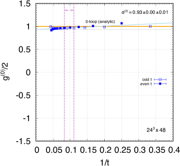
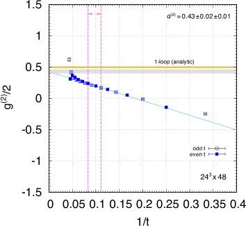
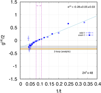
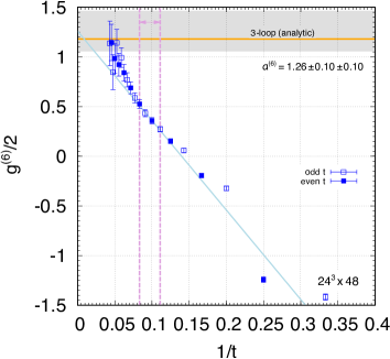
Figure 1: Calculation of the $g$ factor on the $24^{3}\times 48$ lattice. Four points between the dashed lines are used for the extrapolations to $1/t\to 0$. Lines of the extrapolation are drawn by using the central values of $a^{(2n)}$ and $b^{(2n)}$ in Eq. (70).

We show in Fig. 1 the function $g(t)$ in Eq. (49) as a function of $1/t$ for the $24^{3}\times 48$ lattice. The points are shown for $3\leq t<L/2$. At each order, coefficients, $g^{(2n)}(t)/2$, of the expansion,

$${g(t)\over 2}={g^{(0)}(t)\over 2}+{g^{(2)}(t)\over 2}\left({\alpha\over\pi}\right)+{g^{(4)}(t)\over 2}\left({\alpha\over\pi}\right)^{2}+{g^{(6)}(t)\over 2}\left({\alpha\over\pi}\right)^{3}+\cdots,$$ (69)

are plotted. We see the expected behavior discussed in the previous section,

$${g^{(2n)}(t)\over 2}\simeq a^{(2n)}+b^{(2n)}/t,$$ (70)

where deviation can be seen at $1/t\lesssim 1/12\sim 0.08$. We extrapolate to the $t\to\infty$ limit, i.e., $a^{(2n)}$, as follows. We identify the linearly scaling region; the data at too small $t$ are affected by subleading $t$ dependence, whereas those at too large $t$ are contaminated by contributions from backward propagations. We then select the points to be used in the extrapolation to $1/t\to 0$ as $t=T/4-3$, $T/4-2$, $T/4-1$, and $T/4$. We perform two linear extrapolations; one line connects the two even points among these four points, and the other does the odd points. We then take an average of the two extrapolated values. As we discussed before, even and odd points are calculated in a different manner due to vanishing Fourier coefficients by the doubler contributions. We see in the figure that the even and odd points separately behave as linear functions but eventually merge at large $t$. We take the difference between the even and odd extrapolations as a systematic error. By this procedure, one obtains the $g$ factor at a finite lattice spacing. The lines $a^{(2n)}+b^{(2n)}/t$ obtained in this way are shown in the figure. The grey shaded regions are the values of $a^{(2n)}$ with statistical and systematic errors whereas the horizontal lines show the known coefficients by the standard Feynman diagram method:

$$a^{(0)}=1,\quad a^{(2)}=0.5,\quad a^{(4)}=-0.328\dots\quad a^{(6)}=1.18\dots$$ (71)

We see that our parameter choice at $L=24$ is not too far from the continuum limit.

Repeating the same calculations for other sizes of lattices, one can see the $L$ dependence of the $g$ factors. The results are listed in Table 2. The statistical errors are estimated by the jackknife method with the bin size $n_{\rm bin}=10$. With the parameter relations in Eq. (66), it is expected for large $L$ that the values approach to the continuum limit as

$$g(L)\sim g(\infty)+{c\pi\over L},$$ (72)

with an $O(1)$ coefficient, $c$. The coefficient, $c$, however, can have logarithmic dependence on $L$ reflected by the logarithmic UV divergences in the relation between $m_{f}$ and $m$. Since the continuum limit $a\to 0$ should be taken with the physical fermion mass $m_{f}$ fixed, the actual discretization error is $O(m_{f}^{2}a^{2})$ rather than $O(m^{2}a^{2})\sim O(\pi/L)$. The size of the logarithmic correction is controlled by the UV cut-off parameter $\Lambda_{\rm UV}$ in the action. We take $(\Lambda_{\rm UV}a)^{2}=2.0$ which makes the logarithmic correction to be of $O(1)$. For $\Lambda_{\rm UV}a\to\infty$, the continuum limit gets far away as we discuss later.

$L^{3}\times T$	$a^{(0)}$	$a^{(2)}$	$a^{(4)}$	$a^{(6)}$
$12^{3}\times 24$	$0.85(0)(4)$	$0.46(2)(6)$	$-0.54(2)(11)$	$1.14(4)(17)$
$16^{3}\times 32$	$0.90(0)(2)$	$0.45(2)(2)$	$-0.43(3)(6)$	$0.96(6)(6)$
$20^{3}\times 40$	$0.92(0)(1)$	$0.43(2)(2)$	$-0.38(4)(5)$	$1.03(8)(8)$
$24^{3}\times 48$	$0.93(0)(1)$	$0.43(2)(1)$	$-0.28(5)(3)$	$1.26(10)(10)$
(analytic)	1	0.5	$-0.328\dots$	$1.18\dots$

Table 2: Simulation results. Parameters are listed in Table 1. The first and second parentheses represent statistical and systematic errors, respectively. We estimate the total errors as the sum of two numbers. The values in the continuum theory are listed in the last row.

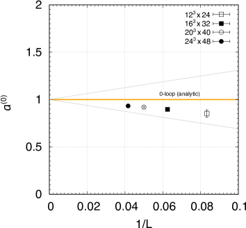
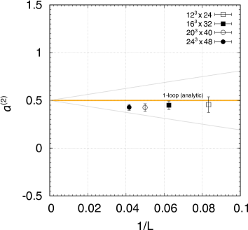
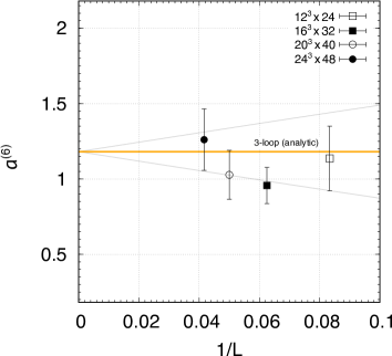
Figure 2: $L$ dependence of the perturbative coefficienets of the $g$ factor on the lattice. $1/L\to 0$ corresponds to the continuum limit by fixing the parameter relations in Eq. (66). The grey lines represent expected sizes of the discretization errors, $\pm(ma)^{2}$.

We show in Fig. 2 the $L$ dependence of the $g$ factor coefficients, $a^{(2n)}$, for each order of perturbations. The horizontal lines are again the known analytic results in the continuum theory. The grey lines represent the typical sizes of the discretization errors, $\pm(ma)^{2}$. We see a good agreement with the analytic results within the expected uncertainties. At the tree level, there is no statistical error even though we use $A_{\mu}^{(0)}$ in Eq. (38), which fluctuates in the Langevin evolutions. This is because at the tree-level $A_{\mu}$ appears only at the external line and its fluctuation is exactly canceled when the photon propagator is removed as in Eq. (44) in each configuration. Also, in the renormalization of the charge in Eq. (32), we use the analytic expression, $Z_{3}^{(0)}(\hat{k}^{2})=e^{-2\hat{k}^{2}/\Lambda_{\rm UV}^{2}}$, for the tree-level value. The deviation from the continuum theory seen in the figure is due to the $O(a^{2})$ correction in the fermion-fermion-photon vertex in the lattice Dirac operator. We do not try to obtain the extrapolated values in the $1/L\to 0$ limit as a reliable estimation seems to require points with larger lattice sizes to control the logarithmic correction of the form $(1/L)\ln L$.

To confirm the validity of our calculation, e.g., the validity of the discretized Langevin steps, we also perform one-loop calculations with the method using Feynman diagrams. First, we compare the wave-function renormalization factor of the photon, $Z_{3}$. We obtain $Z_{3}^{-1}=1.30728+0.563(3)(e^{2}/(4\pi^{2}))+\cdots$ with the stochastic method, whereas the diagrammatic calculation gives $Z_{3}^{-1}=1.30728+0.555891(e^{2}/(4\pi^{2}))+\cdots$. While discrepancy beyond the statistical error is seen in the one-loop coefficient, agreement at the level of a percent is confirmed. The vacuum polarization is obtained by the expansion of the fermion determinant in the stochastic calculation. One may need to increase the number of Langevin steps and/or to generate more noise spinors in Eq. (14) if better precision is necessary. The function $g(t)$ in the $12^{3}\times 24$ lattice with a diagrammatic method is also compared with the stochastic result in Fig. 3 at the one-loop level. We find good consistency within the statistical uncertainties.

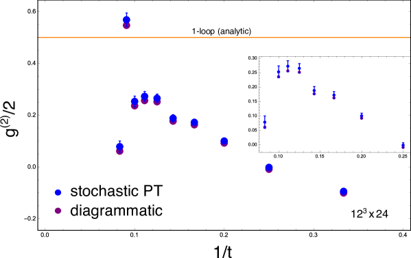
Figure 3: Comparison of the function $g(t)$ at one-loop level between the stochastic perturbation theory (blue) and the conventional lattice perturbation theory using Feynman diagrams (purple) on $12^{3}\times 24$ lattice. Magnified figure is also shown.

The $a^{(2n)}$ factors depend on the UV cutoff parameter $\Lambda_{\rm UV}$ at finite lattice spacings. We show in Fig. 4 the $\Lambda_{\rm UV}$ dependence of the one-loop coefficient, $a^{(2)}$, on the $16^{3}\times 32$ lattice. We take $(\Lambda_{\rm UV}a)^{2}$ to be $2.0$, $8.0$, and $32.0$, respectively, while keeping other parameters to be the same as the ones listed in Table 1. The same numbers of configurations (6,400 confs) are analyzed for each $({\Lambda_{\rm UV}}a)^{2}$. The grey lines represent the typical discretization errors, $\pm(ma)^{2}$, as before. In principle, one can take any value of $\Lambda_{\rm UV}a\neq 0$ as long as we take the continuum limit in the end, but too large $\Lambda_{\rm UV}a$ makes the continuum limit far away as we can see from the figure. This demonstrates that the introduction of a UV regulator is essential in this calculation, otherwise we would need much larger lattice volumes to see the convergence to the continuum values.

One may also employ the gradient flow [43] to reduce the UV fluctuations rather than modifying the action. Also, one can suppress the UV modes by modifying the noise term in the Langevin equation to be momentum dependent as discussed in Ref. [44]. Those two treatments are equivalent to the method of the modified action at the tree level, and may be useful in QCD or in general theories where a gauge invariant UV regularization cannot be simply implemented. An advantage of the modified action is that one can manifestly maintain the equivalence with the path integral formalism, and thus the way to going back to the original theory is theoretically clear.

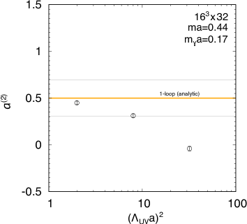
Figure 4: $\Lambda_{\rm UV}$ dependence of the one-loop coefficient, $a^{(2)}$, on the $16^{3}\times 32$ lattice. The grey lines represent the typical size of discretization errors, $\pm(ma)^{2}$, when we ignore the logarithmic correction. Only the statistical errors are shown.

9 IR and finite volume effects

As we modify the QED action to include the finite photon mass, the gauge invariance is broken. In particular, the effects of the photon zero mode should be carefully treated. We also have finite volume effects in the calculation of the function $g(t)$. We discuss those issues in this section.

We first discuss the effects of the photon zero mode. Although we assumed that $\hat{G}_{\mu}$ and $\hat{G}^{\rm(norm)}_{\mu}$ in Eqs. (44) and (45) have the double poles due to the on-shell divergences of the external fermions, they actually have higher poles. These poles show up, in the language of Feynman diagrams, as an IR divergence where internal fermion propagators hit on-shell when the photon loop momentum vanishes. For instance, at one loop, since we have four fermion propagators at most, $\hat{G}_{\mu}$ has a quartic pole. With this higher pole, the functions $\mathcal{F}_{E}(t)$ and $\mathcal{F}_{M}(t)$ behave as $\sim t^{3}z_{*}^{t-2}$ with a prefactor of $O(1/(L^{3}Tm_{\gamma}^{2}))$. This unwanted growth of the functions are worse for smaller $m_{\gamma}$. Moreover, since we fix $m_{\gamma}^{2}\sim 4(\pi/L)^{3}$ in Eq. (67), the effects do not disappear in the $L\to\infty$ limit at large $t$.

However, these seemingly problematic contributions are cancelled in the function $g(t)$ of Eq. (49). This can be understood from the fact that the contributions from the photon zero mode is factorized as an overall factor $\propto e^{-xt^{2}}$ with $x=e^{2}/(2L^{3}Tm_{\gamma}^{2})$ [39, 40] in the fermion two-point functions and the three-point function we consider.

The effects of the backward propagation in the correlation functions are more serious in the extraction of the $g$ factor we developed. For instance in Eq. (47), related to the symmetry of the loop sum under $t\to T-t$, the leading $t$ dependent part should be accompanied with the backward propagating contribution:

$$\mathcal{F}_{E}(t) \sim tz_{*}^{t}e^{-xt^{2}}+(T-t)z_{*}^{(T-t)}e^{-x(T-t)^{2}}$$

$$\sim te^{-Et}e^{-xt^{2}}\left[1+\left(\frac{T}{t}-1\right)e^{-E(T-2t)}e^{-xT(T-2t)}\right]$$

$$=te^{-Et}e^{-xt^{2}}\left[1+\left(\frac{T}{t}-1\right)e^{-E_{0}(T-2t)}\left(1-e^{2}\left(E_{1}+{1\over 2L^{3}m_{\gamma}^{2}}\right)(T-2t)+\cdots\right)\right].$$ (73)

By ignoring the backward propagation, one obtains $\mathcal{F}_{E}(t)\sim te^{-Et}$ up to the $e^{-xt^{2}}$ factor which is to be canceled in the ratio. The extra terms disturb this behavior. In principle, one can fit the function $g(t)$ by using the above expected behavior. Rather than trying such an analysis, for simplicity, we choose a strategy to look for a region of the extrapolation where the extra term is not important. In future works, it is worth trying such an analysis.

The extra contributions are more and more important for higher orders. In the last line, we express the correction term as a perturbative series. The fermion energy as well as the factor of the photon zero mode are expanded as $E=E_{0}+e^{2}E_{1}+\cdots$ and $e^{-xT(T-2t)}=1-(e^{2}/(2L^{3}m_{\gamma}^{2}))(T-2t)+\cdots$, respectively. One can see that the powers of $(T-2t)$ grow as $(T-2t)^{n}$ at the $e^{2n}$ order. Since there is an overall suppression factor $e^{-E_{0}(T-2t)}$, one can avoid this problem for sufficiently large $T$ while keeping the region of extrapolation to be $t\ll T/2$. Nevertheless, for a fixed $T$, there is a certain perturbative order beyond which the extrapolation by Eq. (70) is not reliable.

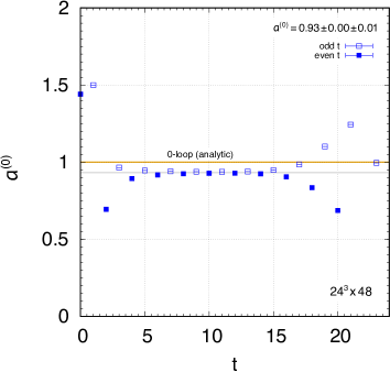
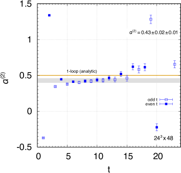
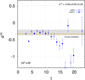
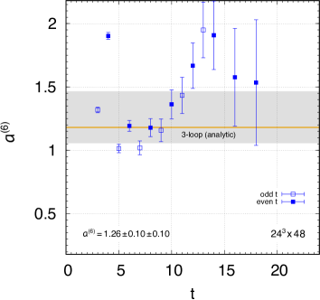
Figure 5: Dependence of the $n$-loop perturbative coefficients $a^{(2n)}$ on the points used in the extrapolation of $g(t)$. The $a^{(2n)}$ factors obtained by the extrapolations based on Eq. (70) by using $g(t)$ at $t$ and $t+2$ are shown. The grey bands correspond to our results in Table 2.

Such a limitation is already observed in Fig. 1, where the deviation from the straight line starts to show up at smaller $t$ for higher orders. In order to visualize the deviation, we show in Fig. 5 the $a^{(2n)}$ factors obtained by the extrapolation of points at $t$ and $t+2$. Up to the two-loop level, we see clear plateaus, which indicate that the results are not significantly sensitive to the range of extrapolations. The plateaus are indeed consistent with our results with the estimated error given in Table 2. At the three-loop order, the plateau seems to start disappearing. A simulation with larger $T$ will be necessary to perform a more reliable estimate, especially for computation beyond three loops.

10 Summary

We apply the numerical stochastic perturbation theory to QED and evaluate the perturbative coefficients of the $g$ factor of the electron up to $O(\alpha^{3})$. We demonstrate that the method reproduces the known results from the diagrammatic method, and expect that it may be able to confirm or predict the higher order perturbative coefficients. Since the method does not rely on the Feynman diagrams, going to higher orders is a matter of computational time and the memory footprint. For example, the increase of the computational cost to accumulate the same number of configurations at the five-loop level is about a factor of two compared to the present work. Although we need more statistics as well as more data points at larger lattice volumes to approach the continuum limit with controlled systematic effects, the results obtained on a small-scale computer in this work are quite encouraging.

The numerical stochastic perturbation theory has been successfully applied to QCD to compute the quantities such as the vacuum energy density and the heavy-quark self-energy, which can be naturally defined on the Euclidean space-time. The challenge we faced in this work is to obtain the physical quantity, $g-2$, defined for an electron on its mass-shell. Thus, an analytic continuation from the Euclidean momentum to the on-shell electron is inevitable. We introduce the Cauchy integral of the vertex function in terms of the imaginary temporal momentum $p_{4}$ and design an appropriate combination, from which the $g$-factor can be obtained at large Euclidean time separations.

The main practical limitation of the method is to separate various energy scales including the electron mass, the external photon momentum and the photon mass. The latter two of these have to be sent to zero in order to obtain the physical result. The photon mass is introduced to avoid an infrared divergence due to finite volume, and it also plays the role to lift the energy of multi-particle states made of an electron and photon so that the single electron state can be easily isolated. Therefore, the extrapolation to the massless photon limit has to be done with great care. In this work, we set the parameters such that these energy scales are separated equally in the logarithmic scale. The systematic error then scales rather slowly, $\sim 1/L$, as a function of the lattice extent $L$. The largest lattice volume in this work is $L=24$; we expect that the simulation at $L\sim 128$ would be possible on the large-scale machines currently used for modern QCD simulations.

For the complete evaluation of the $g-2$ of the electron or the muon, we need to include fermions with different masses to incorporate the mass-dependent contributions. It is straightforward to include those in the Lengiven equation, but having the mass hierarchy as well as the separation of different energy scales poses an extra complication to the parameter setting and extrapolation as described above. We leave such investigations for future works.

Of course, the stochastic method would not replace the diagrammatic computations due to limited accuracy. Especially, for higher orders, in addition to growing statistical uncertainties, the logarithmically enhanced discretization may become an important limiting factor, because they cannot be easily eliminated by numerical extrapolations. Nevertheless, even with, for example, of order of ten percent accuracy, it would provide useful estimate of the higher order coefficients for which the diagrammatic calculation is difficult to reach.

This work provides an evidence that the stochastic quantization method is practically useful in the perturbative calculation of physical quantities, and it may be more effective than the Feynman diagrams at higher loops. We expect that the range of the applications to be much wider than QCD and QED. In general, once we encounter a problem which is sufficiently complicated in the diagrammatic approach, the stochastic method may provide an efficient means to approach.

Appendix A Ward-Takahashi identities

The lattice action with $m_{\gamma}=0$ is invariant under the following BRS transformation:

$$\delta_{\rm BRS}\psi=i\lambda c\psi,$$ (A.1)

$$\delta_{\rm BRS}\bar{\psi}=-i\bar{\psi}\lambda c,$$ (A.2)

$$\delta_{\rm BRS}A_{\mu}=-{1\over e}\lambda\nabla_{\mu}c,$$ (A.3)

$$\delta_{\rm BRS}\bar{c}=-{i\over e}\lambda B,$$ (A.4)

$$\delta_{\rm BRS}c=0,$$ (A.5)

$$\delta_{\rm BRS}B=0.$$ (A.6)

Here $\lambda$ is an anticommuting parameter. The fields $B$, $c$, and $\bar{c}$ are the Nakanishi-Lautrup field, the ghost field, and the anti-ghost field, respectively, with the action:

$$S_{B+c}=\sum_{n}\left[\hat{B}(n)\nabla_{\mu}^{*}\hat{A}_{\mu}(n)-{\xi\over 2}\hat{B}(n)^{2}+i\hat{\bar{c}}(n)\nabla_{\mu}^{*}\nabla_{\mu}\hat{c}(n)\right],$$ (A.7)

where the symbol “$\ \hat{}\$” represents the fields multiplied by the UV regulator, $\hat{\Phi}(n)=e^{-\nabla^{2}/\Lambda_{\rm UV}^{2}}\Phi(n)$. The gauge fixing term is obtained by integrating out the $B$ field. The equation of motion

$$B={1\over\xi}\nabla_{\mu}^{*}A_{\mu},$$ (A.8)

holds as the operator equation, i.e.,

$$\langle B(n){\cal O}_{1}\cdots{\cal O}_{m}\rangle={1\over\xi}\langle\nabla_{\mu}^{*}A_{\mu}(n){\cal O}_{1}\cdots{\cal O}_{m}\rangle,$$ (A.9)

where ${\cal O}$’s are local operators which do not contain $B$. Also, the ghosts are free fields in QED. Therefore,

$$\langle c(n)\bar{c}(m)\rangle=i\int{d^{4}k\over(2\pi)^{4}}{e^{-2\hat{k}^{2}/\Lambda_{\rm UV}^{2}}\over\hat{k}^{2}}e^{ik\cdot(x_{n}-x_{m})}.$$ (A.10)

The BRS symmetry tells us

$$\langle\delta_{\rm BRS}\left(A_{\mu}(n_{1})\bar{c}(n_{2})\right)\rangle=0,$$ (A.11)

and

$$\langle\delta_{\rm BRS}\left(\psi(n_{1})\bar{\psi}(n_{2})\bar{c}(n_{3})\right)\rangle=0.$$ (A.12)

These two equations lead the following Ward-Takahashi identities:

$$\hat{k}_{\nu}{\cal D}_{\mu\nu}(k)={\xi\hat{k}_{\mu}\over\hat{k}^{2}}e^{-2\hat{k}^{2}/\Lambda_{\rm UV}^{2}},$$ (A.13)

$$\hat{k}_{\mu}G_{\mu}(p,k)={e\xi\over\hat{k}^{2}}\left(S(p+k)-S(p)\right)e^{-2\hat{k}^{2}/\Lambda_{\rm UV}^{2}}.$$ (A.14)

Here ${\cal D}_{\mu\nu}$, $S(p)$, and $G_{\mu}(p,k)$ are defined in Eqs. (34), (37), and (38), respectively.

The first identity (A.13) implies that the longitudinal part of the propagator is exact at tree level, and thus

$$\hat{k}_{\mu}{\cal D}^{-1}_{\mu\nu}(k)={\hat{k}^{2}\over\xi}\hat{k}_{\nu}e^{2\hat{k}^{2}/\Lambda_{\rm UV}^{2}}.$$ (A.15)

By using Eqs. (A.14), (A.15) and the definition in Eq. (39), one finds

$$\hat{k}_{\mu}\left(-ie_{\rm P}\Gamma_{\mu}(p,k)\right)=e\kappa\left(S(p)^{-1}-S(p+k)^{-1}\right).$$ (A.16)

The Ward-Takahashi identities are modified when we include the mass term. The identities are

$$\langle\delta_{\rm BRS}\left(A_{\mu}(n_{1})\bar{c}(n_{2})\right)\rangle=\left\langle\sum_{n_{3}}m_{\gamma}^{2}\hat{A}_{\nu}(n_{3})\left(-{1\over e}\lambda\nabla_{\nu}\hat{c}(n_{3})\right)A_{\mu}(n_{1})\bar{c}(n_{2})\right\rangle,$$ (A.17)

and

$$\langle\delta_{\rm BRS}\left(\psi(n_{1})\bar{\psi}(n_{2})\bar{c}(n_{3})\right)\rangle=\left\langle\sum_{n_{4}}m_{\gamma}^{2}\hat{A}_{\nu}(n_{4})\left(-{1\over e}\lambda\nabla_{\nu}\hat{c}(n_{4})\right)\psi(n_{1})\bar{\psi}(n_{2})\bar{c}(n_{3})\right\rangle.$$ (A.18)

These identities lead to

$$\hat{k}_{\mu}{\cal D}_{\mu\nu}(k)={\xi\hat{k}_{\nu}\over\hat{k}^{2}+\xi m_{\gamma}^{2}}e^{-2\hat{k}^{2}/\Lambda_{\rm UV}^{2}},$$ (A.19)

$$\hat{k}_{\mu}G_{\mu}(p,k)={e\xi\over\hat{k}^{2}+\xi m_{\gamma}^{2}}\left(S(p+k)-S(p)\right)e^{-2\hat{k}^{2}/\Lambda_{\rm UV}^{2}}.$$ (A.20)

Again, Eq. (A.19) says that the longitudinal part of the propagator is exact at the tree level. Together with the second identity, one finds that Eq. (A.16) is maintained even with the photon mass term.

Appendix B Numerical integration of the Langevin equation

We are going to solve the following type of equation,

$$\dot{\phi}(n,\tau) =f(n,\tau)+\eta(n,\tau),$$ (B.1)

with the Gaussian noise,

$$\langle\eta(n,\tau)\eta(n^{\prime},\tau^{\prime})\rangle_{\eta}=2\delta_{nn^{\prime}}\delta(\tau-\tau^{\prime}).$$ (B.2)

One can discretize the fictitious time $\tau$ as

$$\phi(n,\tau_{i+1})-\phi(n,\tau_{i})=f(n,\tau_{i})\Delta\tau+\eta(n,\tau_{i})\Delta\tau,$$ (B.3)

with

$$\langle\eta(n,\tau_{i})\eta(n^{\prime},\tau_{j})\rangle_{\eta}=2\delta_{nn^{\prime}}{1\over\Delta\tau}\delta_{ij}.$$ (B.4)

Now $\eta(n,\tau_{i})$ are independent Gaussian noise with the variance

$$\sigma^{2} ={2\over\Delta\tau}.$$ (B.5)

Therefore,

$$\phi(n,\tau_{i+1})-\phi(n,\tau_{i})=f(n,\tau_{i})\Delta\tau+g(n,\tau_{i})\sqrt{2\Delta\tau},$$ (B.6)

where $g(n,\tau_{i})$ are independent Gaussian noises with the variance $\sigma^{2}=1$. By taking the limit of small $\Delta\tau$, one can integrate the Langevin equation.

A simple improvement is possible by using the Runge-Kutta type algorithm [41].

$$\phi(n,\tau_{i+1})-\phi(n,\tau_{i})={1\over 2}\left(f_{1}(n,\tau_{i})+f_{2}(n,\tau_{i})\right)\Delta\tau+g(n,\tau_{i})\sqrt{2\Delta\tau},$$ (B.7)

where

$$f_{1}(n,\tau_{i})=f(n,\tau_{i})\Big{|}_{\phi_{i}},$$ (B.8)

and

$$f_{2}(n,\tau_{i})=f(n,\tau_{i})\Big{|}_{\phi_{i}+f_{1}\Delta\tau+g\sqrt{2\Delta\tau}}.$$ (B.9)

The Gaussian noises are common for Eqs. (B.7) and (B.9).

References

- [1] T. Aoyama, T. Kinoshita, and M. Nio, Theory of the Anomalous Magnetic Moment of the Electron, Atoms, vol. 7, no. 1, p. 28, 2019, doi:10.3390/atoms7010028.
- [2] D. Hanneke, S. Fogwell, and G. Gabrielse, New Measurement of the Electron Magnetic Moment and the Fine Structure Constant, Phys. Rev. Lett., vol. 100, p. 120801, 2008, doi:10.1103/PhysRevLett.100.120801, arXiv:0801.1134 [physics.atom-ph].
- [3] A. Petermann, Fourth order magnetic moment of the electron, Helv. Phys. Acta, vol. 30, pp. 407–408, 1957, doi:10.5169/seals-112823.
- [4] C. M. Sommerfield, Magnetic Dipole Moment of the Electron, Phys. Rev., vol. 107, pp. 328–329, 1957, doi:10.1103/PhysRev.107.328.
- [5] J. S. Schwinger, On Quantum electrodynamics and the magnetic moment of the electron, Phys. Rev., vol. 73, pp. 416–417, 1948, doi:10.1103/PhysRev.73.416.
- [6] S. Laporta and E. Remiddi, The Analytical value of the electron (g-2) at order alpha**3 in QED, Phys. Lett. B, vol. 379, pp. 283–291, 1996, doi:10.1016/0370-2693(96)00439-X, arXiv:hep-ph/9602417.
- [7] P. Cvitanovic and T. Kinoshita, Sixth Order Magnetic Moment of the electron, Phys. Rev. D, vol. 10, p. 4007, 1974, doi:10.1103/PhysRevD.10.4007.
- [8] T. Kinoshita and P. Cvitanovic, Sixth-order radiative corrections to the electron magnetic moment, Phys. Rev. Lett., vol. 29, pp. 1534–1537, 1972, doi:10.1103/PhysRevLett.29.1534.
- [9] M. J. Levine and J. Wright, Anomalous magnetic moment of the electron, Phys. Rev. D, vol. 8, pp. 3171–3179, 1973, doi:10.1103/PhysRevD.8.3171.
- [10] R. Carroll and Y. Yao, Alpha-to-the-3 contributions to the anomalous magnetic moment of an electron in the mass-operator formalism, Phys. Lett. B, vol. 48, pp. 125–127, 1974, doi:10.1016/0370-2693(74)90659-5.
- [11] R. Carroll, Mass Operator Calculation of the electron G-Factor, Phys. Rev. D, vol. 12, p. 2344, 1975, doi:10.1103/PhysRevD.12.2344.
- [12] T. Kinoshita, New value of the alpha**3 electron anomalous magnetic moment, Phys. Rev. Lett., vol. 75, pp. 4728–4731, 1995, doi:10.1103/PhysRevLett.75.4728.
- [13] T. Aoyama, M. Hayakawa, T. Kinoshita, M. Nio, and N. Watanabe, Eighth-Order Vacuum-Polarization Function Formed by Two Light-by-Light-Scattering Diagrams and its Contribution to the Tenth-Order Electron g-2, Phys. Rev. D, vol. 78, p. 053005, 2008, doi:10.1103/PhysRevD.78.053005, arXiv:0806.3390 [hep-ph].
- [14] T. Aoyama, M. Hayakawa, T. Kinoshita, and M. Nio, Tenth-Order Lepton Anomalous Magnetic Moment: Second-Order Vertex Containing Two Vacuum Polarization Subdiagrams, One Within the Other, Phys. Rev. D, vol. 78, p. 113006, 2008, doi:10.1103/PhysRevD.78.113006, arXiv:0810.5208 [hep-ph].
- [15] T. Aoyama, M. Hayakawa, T. Kinoshita, and M. Nio, Tenth-order lepton g-2: Contribution of some fourth-order radiative corrections to the sixth-order g-2 containing light-by-light-scattering subdiagrams, Phys. Rev. D, vol. 82, p. 113004, 2010, doi:10.1103/PhysRevD.82.113004, arXiv:1009.3077 [hep-ph].
- [16] T. Aoyama, K. Asano, M. Hayakawa, T. Kinoshita, M. Nio, and N. Watanabe, Tenth-order lepton g-2: Contribution from diagrams containing sixth-order light-by-light-scattering subdiagram internally, Phys. Rev. D, vol. 81, p. 053009, 2010, doi:10.1103/PhysRevD.81.053009, arXiv:1001.3704 [hep-ph].
- [17] T. Aoyama, M. Hayakawa, T. Kinoshita, and M. Nio, Proper Eighth-Order Vacuum-Polarization Function and its Contribution to the Tenth-Order Lepton g-2, Phys. Rev. D, vol. 83, p. 053003, 2011, doi:10.1103/PhysRevD.83.053003, arXiv:1012.5569 [hep-ph].
- [18] T. Aoyama, M. Hayakawa, T. Kinoshita, and M. Nio, Tenth-Order QED Lepton Anomalous Magnetic Moment — Eighth-Order Vertices Containing a Second-Order Vacuum Polarization, Phys. Rev. D, vol. 85, p. 033007, 2012, doi:10.1103/PhysRevD.85.033007, arXiv:1110.2826 [hep-ph].
- [19] T. Aoyama, M. Hayakawa, T. Kinoshita, and M. Nio, Tenth-Order QED contribution to Lepton Anomalous Magnetic Moment - Fourth-Order Vertices Containing Sixth-Order Vacuum-Polarization Subdiagrams, Phys. Rev. D, vol. 83, p. 053002, 2011, doi:10.1103/PhysRevD.83.053002, arXiv:1101.0459 [hep-ph].
- [20] T. Aoyama, M. Hayakawa, T. Kinoshita, and M. Nio, Tenth-Order Lepton Anomalous Magnetic Moment – Sixth-Order Vertices Containing Vacuum-Polarization Subdiagrams, Phys. Rev. D, vol. 84, p. 053003, 2011, doi:10.1103/PhysRevD.84.053003, arXiv:1105.5200 [hep-ph].
- [21] T. Aoyama, M. Hayakawa, T. Kinoshita, and M. Nio, Tenth-Order QED Contribution to the Lepton Anomalous Magnetic Moment – Sixth-Order Vertices Containing an Internal Light-by-Light-Scattering Subdiagram, Phys. Rev. D, vol. 85, p. 093013, 2012, doi:10.1103/PhysRevD.85.093013, arXiv:1201.2461 [hep-ph].
- [22] T. Aoyama, M. Hayakawa, T. Kinoshita, and M. Nio, Tenth-Order QED Contribution to the Electron g-2 and an Improved Value of the Fine Structure Constant, Phys. Rev. Lett., vol. 109, p. 111807, 2012, doi:10.1103/PhysRevLett.109.111807, arXiv:1205.5368 [hep-ph].
- [23] T. Aoyama, T. Kinoshita, and M. Nio, Revised and Improved Value of the QED Tenth-Order Electron Anomalous Magnetic Moment, Phys. Rev. D, vol. 97, no. 3, p. 036001, 2018, doi:10.1103/PhysRevD.97.036001, arXiv:1712.06060 [hep-ph].
- [24] S. Volkov, Calculating the five-loop QED contribution to the electron anomalous magnetic moment: Graphs without lepton loops, Phys. Rev. D, vol. 100, no. 9, p. 096004, 2019, doi:10.1103/PhysRevD.100.096004, arXiv:1909.08015 [hep-ph].
- [25] F. Di Renzo, G. Marchesini, P. Marenzoni, and E. Onofri, Lattice perturbation theory on the computer, Nucl. Phys. B Proc. Suppl., vol. 34, pp. 795–798, 1994, doi:10.1016/0920-5632(94)90517-7.
- [26] F. Di Renzo, E. Onofri, G. Marchesini, and P. Marenzoni, Four loop result in SU(3) lattice gauge theory by a stochastic method: Lattice correction to the condensate, Nucl. Phys. B, vol. 426, pp. 675–685, 1994, doi:10.1016/0550-3213(94)90026-4, arXiv:hep-lat/9405019.
- [27] F. Di Renzo and L. Scorzato, Fermionic loops in numerical stochastic perturbation theory, Nucl. Phys. B Proc. Suppl., vol. 94, pp. 567–570, 2001, doi:10.1016/S0920-5632(01)00868-4, arXiv:hep-lat/0010064.
- [28] F. Di Renzo, V. Miccio, and L. Scorzato, Unquenched numerical stochastic perturbation theory, Nucl. Phys. B Proc. Suppl., vol. 119, pp. 1003–1005, 2003, doi:10.1016/S0920-5632(03)01744-4, arXiv:hep-lat/0209018.
- [29] F. Di Renzo and L. Scorzato, Numerical stochastic perturbation theory for full QCD, JHEP, vol. 10, p. 073, 2004, doi:10.1088/1126-6708/2004/10/073, arXiv:hep-lat/0410010.
- [30] G. Parisi and Y.-s. Wu, Perturbation Theory Without Gauge Fixing, Sci. Sin., vol. 24, p. 483, 1981.
- [31] G. S. Bali, C. Bauer, and A. Pineda, Perturbative expansion of the plaquette to in four-dimensional SU(3) gauge theory, Phys. Rev. D, vol. 89, p. 054505, 2014, doi:10.1103/PhysRevD.89.054505, arXiv:1401.7999 [hep-ph].
- [32] L. Del Debbio, F. Di Renzo, and G. Filaci, Large-order NSPT for lattice gauge theories with fermions: the plaquette in massless QCD, Eur. Phys. J. C, vol. 78, no. 11, p. 974, 2018, doi:10.1140/epjc/s10052-018-6458-9, arXiv:1807.09518 [hep-lat].
- [33] G. S. Bali, C. Bauer, and A. Pineda, Model-independent determination of the gluon condensate in four-dimensional SU(3) gauge theory, Phys. Rev. Lett., vol. 113, p. 092001, 2014, doi:10.1103/PhysRevLett.113.092001, arXiv:1403.6477 [hep-ph].
- [34] D. Zwanziger, Covariant Quantization of Gauge Fields Without Gribov Ambiguity, Nucl. Phys. B, vol. 192, p. 259, 1981, doi:10.1016/0550-3213(81)90202-9.
- [35] U. M. Heller and F. Karsch, One Loop Perturbative Calculation of Wilson Loops on Finite Lattices, Nucl. Phys. B, vol. 251, pp. 254–278, 1985, doi:10.1016/0550-3213(85)90261-5.
- [36] M. Hayakawa and S. Uno, QED in finite volume and finite size scaling effect on electromagnetic properties of hadrons, Prog. Theor. Phys., vol. 120, pp. 413–441, 2008, doi:10.1143/PTP.120.413, arXiv:0804.2044 [hep-ph].
- [37] Z. Davoudi, J. Harrison, A. Jüttner, A. Portelli, and M. J. Savage, Theoretical aspects of quantum electrodynamics in a finite volume with periodic boundary conditions, Phys. Rev. D, vol. 99, no. 3, p. 034510, 2019, doi:10.1103/PhysRevD.99.034510, arXiv:1810.05923 [hep-lat].
- [38] M. Luscher and P. Weisz, Efficient Numerical Techniques for Perturbative Lattice Gauge Theory Computations, Nucl. Phys. B, vol. 266, p. 309, 1986, doi:10.1016/0550-3213(86)90094-5.
- [39] M. G. Endres, A. Shindler, B. C. Tiburzi, and A. Walker-Loud, Massive photons: an infrared regularization scheme for lattice QCD+QED, Phys. Rev. Lett., vol. 117, no. 7, p. 072002, 2016, doi:10.1103/PhysRevLett.117.072002, arXiv:1507.08916 [hep-lat].
- [40] M. G. Endres, A. Shindler, B. C. Tiburzi, and A. Walker-Loud, Photon mass term as an IR regularization for QCD+QED on the lattice, PoS, vol. LATTICE2015, p. 078, 2016, doi:10.22323/1.251.0078, arXiv:1512.08983 [hep-lat].
- [41] E. Helfand, Numerical integration of stochastic differential equations, The Bell System Techinical Journal, vol. 58, no. 10, p. 2289, 1979.
- [42] G. Batrouni, G. Katz, A. S. Kronfeld, G. Lepage, B. Svetitsky, and K. Wilson, Langevin Simulations of Lattice Field Theories, Phys. Rev. D, vol. 32, p. 2736, 1985, doi:10.1103/PhysRevD.32.2736.
- [43] M. Lüscher, Properties and uses of the Wilson flow in lattice QCD, JHEP, vol. 08, p. 071, 2010, doi:10.1007/JHEP08(2010)071, arXiv:1006.4518 [hep-lat]. [Erratum: JHEP 03, 092 (2014)].
- [44] Z. Bern, M. B. Halpern, and N. G. Kalivas, Heat Kernel Regularization of Gauge Theory, Phys. Rev. D, vol. 35, p. 753, 1987, doi:10.1103/PhysRevD.35.753.