Smoothing and Shrinking the Sparse Seq2Seq Search Space

Abstract

Current sequence-to-sequence models are trained to minimize cross-entropy and use softmax to compute the locally normalized probabilities over target sequences. While this setup has led to strong results in a variety of tasks, one unsatisfying aspect is its length bias: models give high scores to short, inadequate hypotheses and often make the empty string the argmax—the so-called cat got your tongue problem. Recently proposed entmax-based sparse sequence-to-sequence models present a possible solution, since they can shrink the search space by assigning zero probability to bad hypotheses, but their ability to handle word-level tasks with transformers has never been tested. In this work, we show that entmax-based models effectively solve the cat got your tongue problem, removing a major source of model error for neural machine translation. In addition, we generalize label smoothing, a critical regularization technique, to the broader family of Fenchel-Young losses, which includes both cross-entropy and the entmax losses. Our resulting label-smoothed entmax loss models set a new state of the art on multilingual grapheme-to-phoneme conversion and deliver improvements and better calibration properties on cross-lingual morphological inflection and machine translation for 6 language pairs.

1 Introduction

Sequence-to-sequence models (seq2seq: Sutskever et al., 2014; Bahdanau et al., 2015; Vaswani et al., 2017) have become a powerful and flexible tool for a variety of NLP tasks, including machine translation (MT), morphological inflection (MI; Faruqui et al., 2016), and grapheme-to-phoneme conversion (G2P; Yao and Zweig, 2015). These models often perform well, but they have a bias that favors short hypotheses. This bias is problematic: it has been pointed out as the cause (Koehn and Knowles, 2017; Yang et al., 2018; Murray and Chiang, 2018) of the beam search curse, in which increasing the width of beam search actually decreases performance on neural machine translation (NMT). Further illustrating the severity of the problem, Stahlberg and Byrne (2019) showed that the highest-scoring target sequence in NMT is often the empty string, a phenomenon they dubbed the cat got your tongue problem. These results are undesirable because they show that NMT models’ performance depends on the search errors induced by a narrow beam. It would be preferable for models to assign higher scores to good translations than to bad ones, rather than to depend on search errors to make up for model errors.

The most common way to alleviate this shortcoming is by altering the decoding objective (Wu et al., 2016; He et al., 2016; Yang et al., 2018; Meister et al., 2020a), but this does not address the underlying problem: the model overestimates the probability of implausible hypotheses. Other solutions use alternate training strategies (Murray and Chiang, 2018; Shen et al., 2016), but it would be preferable not to change the training algorithm.

In this paper, we propose a solution based on sparse seq2seq models (Peters et al., 2019), which replace the output softmax (Bridle, 1990) with the entmax transformation. Entmax, unlike softmax, can learn locally sparse distributions over the target vocabulary. This allows a sparse model to shrink the search space: that is, it can learn to give inadequate hypotheses zero probability, instead of counting on beam search to prune them. This has already been demonstrated for MI, where the set of possible hypotheses is often small enough to make beam search exact (Peters et al., 2019; Peters and Martins, 2019). We extend this analysis to MT: although exact beam search is not possible for this large vocabulary task, we show that entmax models prune many inadequate hypotheses, effectively solving the cat got your tongue problem.

Despite this useful result, one drawback of entmax is that it is not compatible with label smoothing (Szegedy et al., 2016), a useful regularization technique that is widely used for transformers (Vaswani et al., 2017). We solve this problem by generalizing label smoothing from the cross-entropy loss to the wider class of Fenchel-Young losses (Blondel et al., 2020), which includes the entmax loss as a particular case. We show that combining label smoothing with entmax loss improves results on both character- and word-level tasks while keeping the model sparse. We note that, although label smoothing improves calibration, it also exacerbates the cat got your tongue problem regardless of loss function.

To sum up, we make the following contributions:

• We show empirically that models trained with entmax loss rarely assign nonzero probability to the empty string, demonstrating that entmax loss is an elegant way to remove a major class of NMT model errors.

• We generalize label smoothing from the cross-entropy loss to the wider class of Fenchel-Young losses, exhibiting a formulation for label smoothing which, to our knowledge, is novel.

• We show that Fenchel-Young label smoothing with entmax loss is highly effective on both character- and word-level tasks. Our technique allows us to set a new state of the art on the SIGMORPHON 2020 shared task for multilingual G2P (Gorman et al., 2020). It also delivers improvements for crosslingual MI from SIGMORPHON 2019 (McCarthy et al., 2019) and for MT on IWSLT 2017 German $\leftrightarrow$ English (Cettolo et al., 2017), KFTT Japanese $\leftrightarrow$ English (Neubig, 2011), and WMT 2016 Romanian $\leftrightarrow$ English (Bojar et al., 2016) compared to a baseline with unsmoothed labels.

2 Background

A seq2seq model learns a probability distribution $p_{\boldsymbol{\theta}}(y\mid x)$ over sequences $y$ from a target vocabulary $V$, conditioned on a source sequence $x$. This distribution is then used at decoding time to find the most likely sequence $\hat{y}$:

$$\hat{y}=\operatorname*{\mathsf{argmax}}_{y\in V^{*}}p_{\boldsymbol{\theta}}(y\mid x),$$ (1)

where $V^{*}$ is the Kleene closure of $V$. This is an intractable problem; seq2seq models depend on heuristic search strategies, most commonly beam search (Reddy et al., 1977). Most seq2seq models are locally normalized, with probabilities that decompose by the chain rule:

$$p_{\boldsymbol{\theta}}(y\mid x)=\prod_{i=1}^{|y|}p_{\boldsymbol{\theta}}(y_{i}\mid x,y_{<i}).$$ (2)

This factorization implies that the probability of a hypothesis being generated is monotonically nonincreasing in its length, which favors shorter sequences. This phenomenon feeds the beam search curse because short hypotheses are pruned from a narrow beam but survive a wider one.

The conditional distribution $p_{\boldsymbol{\theta}}(y_{i}\mid x,y_{<i})$ is obtained by first computing a vector of scores (or “logits”) $\boldsymbol{z}=\boldsymbol{f}_{\boldsymbol{\theta}}(x,y_{<i})\in\mathbb{R}^{|V|}$, where $\boldsymbol{f}_{\boldsymbol{\theta}}$ is parameterized by a neural network, and then applying a transformation $\pi:\mathbb{R}^{|V|}\rightarrow\triangle^{|V|}$, which maps scores to the probability simplex $\triangle^{|V|}:=\{\boldsymbol{p}\in\mathbb{R}^{|V|}\colon\boldsymbol{p}\geq 0,\|\boldsymbol{p}\|_{1}=1\}$. The usual choice for $\pi$ is softmax (Bridle, 1990), which returns strictly positive values, ensuring that all sequences $\in V^{*}$ have nonzero probability. Coupled with the short sequence bias, this causes significant model error.

Sparse seq2seq models.

In a sparse model, the output softmax is replaced by a transformation $\pi$ from the entmax family (Peters et al., 2019). Like softmax, entmax transformations return a vector in the simplex and are differentiable (almost) everywhere. However, unlike softmax, they are capable of producing sparse probability distributions. Concretely, this is done by using the so-called “$\beta$-exponential function” (Tsallis, 1988) in place of the exponential, where $\beta\geq 0$:

$$\exp_{\beta}(v):=\left\{\begin{array}[]{ll}[1+(1-\beta)v]_{+}^{1/(1-\beta)},&\beta\neq 1\\ \exp(v),&\beta=1.\end{array}\right.$$ (3)

The $\beta$-exponential function converges to the regular exponential when $\beta\rightarrow 1$. Entmax models assume that $p(y_{i}\mid x,y_{<i})$ results from an $\alpha$-entmax transformation of the scores $\boldsymbol{z}$, defined as

$$[\alpha\text{-}\mathsf{entmax}(\boldsymbol{z})]_{y}:=\exp_{2-\alpha}(z_{y}-\tau_{\alpha}(\boldsymbol{z})),$$ (4)

where $\tau_{\alpha}(\boldsymbol{z})$ is a constant which ensures normalization. When $\alpha=1$, (4) turns to a regular exponential function and $\tau_{1}(\boldsymbol{z})=\log\sum_{y^{\prime}=1}^{|V|}\exp(z_{y^{\prime}})$ is the log-partition function, recovering softmax. When $\alpha=2$, we recover sparsemax (Martins and Astudillo, 2016). For $\alpha\in\{1.5,2\}$, fast algorithms to compute (4) are available which are almost as fast as evaluating softmax. For other values of $\alpha$, slower bisection algorithms exist.

Entmax transformations are sparse for any $\alpha>1$, with higher values tending to produce sparser outputs. This sparsity allows a model to assign exactly zero probability to implausible hypotheses. For tasks where there is only one correct target sequence, this often allows the model to concentrate all probability mass into a small set of hypotheses, making search exact (Peters and Martins, 2019). This is not possible for open-ended tasks like machine translation, but the model is still locally sparse, assigning zero probability to many hypotheses. These hypotheses will never be selected at any beam width.

Fenchel-Young Losses.

Inspired by the softmax generalization above, Blondel et al. (2020) provided a tool for constructing a convex loss function. Let $\Omega:\triangle^{|V|}\rightarrow\mathbb{R}$ be a strictly convex regularizer which is symmetric, i.e., $\Omega(\Pi\boldsymbol{p})=\Omega(\boldsymbol{p})$ for any permutation $\Pi$ and any $\boldsymbol{p}\in\triangle^{|V|}$. Equipped with $\Omega$, we can define a regularized prediction function $\hat{\pi}_{\Omega}:\mathbb{R}^{|V|}\rightarrow\triangle^{|V|}$, with this form:

$$\hat{\pi}_{\Omega}(\boldsymbol{z})=\operatorname*{\mathsf{argmax}}_{\boldsymbol{p}\in\triangle^{|V|}}\boldsymbol{z}^{\top}\boldsymbol{p}-\Omega(\boldsymbol{p})$$ (5)

where $\boldsymbol{z}\in\mathbb{R}^{|V|}$ is the vector of label scores (logits) and $\Omega:\triangle^{|V|}\rightarrow\mathbb{R}$ is a regularizer. Equation 5 recovers both softmax and entmax with particular choices of $\Omega$: the negative Shannon entropy, $\Omega(\boldsymbol{p})=\sum_{y\in{V}}p_{y}\log p_{y}$, recovers the variational form of softmax (Wainwright and Jordan, 2008), while the negative Tsallis entropy (Tsallis, 1988) with parameter $\alpha$, defined as

$$\Omega_{\alpha}(\boldsymbol{p})=\left\{\begin{array}[]{ll}\frac{1}{\alpha(\alpha-1)}\left(\sum_{y\in V}p_{y}^{\alpha}-1\right),&\text{if $\alpha\neq 1$}\\ \sum_{y\in V}p_{y}\log p_{y},&\text{if $\alpha=1$,}\end{array}\right.$$ (6)

recovers the $\alpha$-entmax transformation in (4), as shown by Peters et al. (2019).

Given the choice of $\Omega$, the Fenchel-Young loss function $L_{\Omega}$ is defined as

$$L_{\Omega}(\boldsymbol{z};\boldsymbol{q}):=\Omega^{*}(\boldsymbol{z})+\Omega(\boldsymbol{q})-\boldsymbol{z}^{\top}\boldsymbol{q},$$ (7)

where $\boldsymbol{q}$ is a target distribution, most commonly a one-hot vector indicating the gold label, $\boldsymbol{q}=\boldsymbol{e}_{y^{*}}=[0,\ldots,0,\underbrace{1}_{\text{$y^{*}$-th entry}},0,\ldots,0]$, and $\Omega^{*}$ is the convex conjugate of $\Omega$, defined variationally as:

$$\Omega^{*}(\boldsymbol{z}):=\max_{\boldsymbol{p}\in\triangle^{|V|}}\boldsymbol{z}^{\top}\boldsymbol{p}-\Omega(\boldsymbol{p}).$$ (8)

The name stems from the Fenchel-Young inequality, which states that the quantity (7) is non-negative (Borwein and Lewis, 2010, Prop. 3.3.4). When $\Omega$ is the generalized negative entropy, the loss (7) becomes the Kullback-Leibler divergence between $\boldsymbol{q}$ and $\operatorname*{\mathsf{softmax}}(\boldsymbol{z})$ (KL divergence; Kullback and Leibler, 1951), which equals the cross-entropy when $\boldsymbol{q}$ is a one-hot vector. More generally, if $\Omega\equiv\Omega_{\alpha}$ is the negative Tsallis entropy (6), we obtain the $\alpha$-entmax loss (Peters et al., 2019).

Fenchel-Young losses have nice properties for training neural networks with backpropagation: they are non-negative, convex, and differentiable as long as $\Omega$ is strictly convex (Blondel et al., 2020, Prop. 2). Their gradient is

$$\nabla_{\boldsymbol{z}}L_{\Omega}(\boldsymbol{z};\boldsymbol{q})=\hat{\pi}_{\Omega}(\boldsymbol{z})-\boldsymbol{q},$$ (9)

which generalizes the gradient of the cross-entropy loss. Figure 1 illustrates particular cases of Fenchel-Young losses considered in this paper.

Figure 1: Diagram illustrating Fenchel-Young losses and the particular case of $\alpha$-entmax family. The case $\alpha=1$ corresponds to softmax and the cross-entropy loss, $\alpha=2$ to the sparsemax loss, and $\alpha=1.5$ to the 1.5-entmax loss. Any choice of $\alpha>1$ (in blue) can lead to sparse distributions.

3 Fenchel-Young Label Smoothing

Label smoothing (Szegedy et al., 2016) has become a popular technique for regularizing the output of a neural network. The intuition behind it is that using the gold target labels from the training set can lead to overconfident models. To overcome this, label smoothing redistributes probability mass from the gold label to the other target labels. When the redistribution is uniform, Pereyra et al. (2017) and Meister et al. (2020b) pointed out that this is equivalent (up to scaling and adding a constant) to adding a second term to the loss that computes the KL divergence $D_{\text{KL}}(\boldsymbol{u}\|\boldsymbol{p}_{\boldsymbol{\theta}})$ between a uniform distribution $\boldsymbol{u}$ and the model distribution $\boldsymbol{p}_{\boldsymbol{\theta}}$. While it might seem appealing to add a similar KL regularizer to a Fenchel-Young loss, this is not possible when $\boldsymbol{p}_{\boldsymbol{\theta}}$ contains zeroes because the KL divergence term becomes infinite. This makes vanilla label smoothing incompatible with sparse models. Fortunately, there is a more natural generalization of label smoothing to Fenchel-Young losses. For $\epsilon\in[0,1]$, we define the Fenchel-Young label smoothing loss as follows:

$$L_{\Omega,\epsilon}(\boldsymbol{z},\boldsymbol{e}_{y^{*}}):=L_{\Omega}(\boldsymbol{z},(1-\epsilon)\boldsymbol{e}_{y^{*}}+\epsilon\boldsymbol{u}).$$ (10)

The intuition is the same as in cross-entropy label smoothing: the target one-hot vector is mixed with a uniform distribution.

This simple definition leads to the following result, proved in Appendix A: The Fenchel-Young label smoothing loss can be written as

$$L_{\Omega,\epsilon}(\boldsymbol{z},\boldsymbol{e}_{y^{*}})=L_{\Omega}(\boldsymbol{z},\boldsymbol{e}_{y^{*}})+\epsilon(z_{y^{*}}-\bar{z})+C,$$ (11)

where $C=-\Omega(\boldsymbol{e}_{y^{*}})+\Omega((1-\epsilon)\boldsymbol{e}_{y^{*}}+\epsilon\boldsymbol{u})$ is a constant which does not depend on $\boldsymbol{z}$, and $\bar{z}:=\boldsymbol{u}^{\top}\boldsymbol{z}$ is the average of the logits. Furthermore, up to a constant, we also have

$$L_{\Omega,\epsilon}(\boldsymbol{z},\boldsymbol{e}_{y^{*}})\propto L_{\Omega}(\boldsymbol{z},\boldsymbol{e}_{y^{*}})+\lambda L_{\Omega}(\boldsymbol{z},\boldsymbol{u}),$$ (12)

where $\lambda=\frac{\epsilon}{1-\epsilon}$.

The first expression (11) shows that, up to a constant, the smoothed Fenchel-Young loss equals the original loss plus a linear regularizer $\epsilon(z_{y^{*}}-\bar{z})$. While this regularizer can be positive or negative, we show in Appendix A that its sum with the original loss $L_{\Omega}(\boldsymbol{z},\boldsymbol{e}_{y^{*}})$ is always non-negative – intuitively, if the score $z_{y^{*}}$ is below the average, resulting in negative regularization, the unregularized loss will also be larger, and the two terms balance each other. Figure 2 shows the effect of this regularization in the graph of the loss – we see that a correct prediction is linearly penalized with a slope of $\epsilon$; the larger the confidence, the larger the penalty. In particular, when $\Omega$ is the Shannon negentropy, this result shows a simple expression for vanilla label smoothing which, to the best of our knowledge, is novel. The second expression (12) shows that it can also be seen as a form of regularization towards the uniform distribution. When $-\Omega$ is the Shannon entropy, the regularizer becomes a KL divergence and we obtain the interpretation of label smoothing for cross-entropy provided by Pereyra et al. (2017) and Meister et al. (2020b). Therefore, the same interpretation holds for the entire Fenchel-Young family if the regularization uses the corresponding Fenchel-Young loss with respect to a uniform.

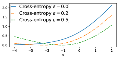
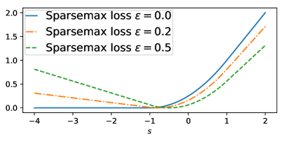
Figure 2: Fenchel-Young label smoothing with various $\epsilon$ values in the two-dimensional case for the cross-entropy loss (left) and sparsemax loss (right). In both cases we define $s=z_{2}-z_{1}$ and assume $y^{*}=1$.

Gradient of Fenchel-Young smoothed loss.

From Prop. 3 and Equation 9, we immediately obtain the following expression for the gradient of the smoothed loss:

$$\nabla_{\boldsymbol{z}}L_{\Omega,\epsilon}(\boldsymbol{z},\boldsymbol{e}_{y^{*}})=$$ (13)

$$= \nabla_{\boldsymbol{z}}L_{\Omega}(\boldsymbol{z},\boldsymbol{e}_{y^{*}})+\epsilon(\boldsymbol{e}_{y^{*}}-\boldsymbol{u})$$

$$= \hat{\pi}_{\Omega}(\boldsymbol{z})-(1-\epsilon)\boldsymbol{e}_{y^{*}}-\epsilon\boldsymbol{u},$$

that is, the computation of this gradient is straightforward by adding a constant vector to the original gradient of the Fenchel-Young loss; as the latter, it only requires the ability of computing the $\hat{\pi}_{\Omega}$ transformation, which is efficient in the entmax case as shown by Peters et al. (2019). Note that, unlike the gradient of the original entmax loss, the gradient of its smoothed version is not sparse (in the sense that it will not contain many zeroes); however, since $\boldsymbol{u}$ is the uniform distribution, it will contain many constant terms with value $-\epsilon/{|V|}$.

4 Experiments

We trained seq2seq models for three tasks: multilingual G2P, crosslingual MI, and MT. These tasks present very different challenges. In G2P and MI, character-level vocabularies are small and there is usually only one correct target sequence. The relative simplicity of these tasks is offset by the small quantity of training data and the strict evaluation: the model must produce exactly the right sequence. This tests Fenchel-Young label smoothing’s ability to learn exactly in a low-resource setting. On the other hand, MT is trained with much larger corpora and evaluated with less strict metrics, but uses subword vocabularies with sizes in the tens of thousands and has to manage more ambiguity because sentences typically have many correct translations.

In all tasks, we vary two hyperparameters:

• Entmax Loss $\alpha$: this influences the sparsity of the probability distributions the model returns, with $\alpha=1$ recovering cross-entropy and larger $\alpha$ values encouraging sparser distributions. We use $\alpha\in\{1,1.5,2\}$ for G2P and MI, and $\alpha\in\{1,1.5\}$ for MT.

• Fenchel-Young Label Smoothing $\epsilon$: higher values give more weight to the uniform smoothing distribution, discouraging sparsity. We use $\epsilon\in\{0,0.01,0.02,\dots,0.15\}$ for G2P, $\epsilon\in\{0,0.01,0.05,0.1\}$ for MI, and $\epsilon\in\{0,0.01,0.1\}$ for MT.

We trained all models with early stopping for a maximum of 30 epochs for MI and 100 epochs otherwise, keeping the best checkpoint according to a task-specific validation metric: Phoneme Error Rate for G2P, average Levenshtein distance for MI, and detokenized BLEU score for MT. At test time, we decoded with a beam width of 5. Our PyTorch code (Paszke et al., 2017) is based on JoeyNMT (Kreutzer et al., 2019) and the entmax implementation from the entmax package.

4.1 Multilingual G2P

		Single		Ensemble
$\alpha$	$\epsilon$	WER $\downarrow$	PER $\downarrow$	WER $\downarrow$	PER $\downarrow$
1	0	18.14 $\pm$ 2.87	3.95 $\pm$ 1.24	14.74	2.96
	0.15	15.55 $\pm$ 0.48	3.09 $\pm$ 0.10	13.87	2.77
1.5	0	15.25 $\pm$ 0.25	3.05 $\pm$ 0.03	13.79	2.77
	0.04	14.18 $\pm$ 0.24	2.86 $\pm$ 0.05	13.47	2.69
2	0	15.08 $\pm$ 0.28	3.04 $\pm$ 0.06	13.84	2.75
	0.04	14.17 $\pm$ 0.20	2.88 $\pm$ 0.04	13.51	2.73
(Yu et al., 2020)				13.81	2.76

Table 1: Multilingual G2P results on the SIGMORPHON 2020 Task 1 test set, macro-averaged across languages. Numbers in the Single column are the average of five independent model runs. The same models are used for the ensembles. Note that $\alpha=1$ and $\alpha=2$ recover cross-entropy and sparsemax loss, respectively.

Data.

We use the data from SIGMORPHON 2020 Task 1 (Gorman et al., 2020), which includes 3600 training examples in each of 15 languages. We train a single multilingual model (following Peters and Martins, 2020) which must learn to apply spelling rules from several writing systems.

Training.

Our models are similar to Peters and Martins (2020)’s RNNs, but with entmax 1.5 attention, and language embeddings only in the source.

Results.

Multilingual G2P results are shown in Table 1, along with the best previous result (Yu et al., 2020). We report two error metrics, each of which is computed per-language and averaged:

• Word Error Rate (WER) is the percentage of hypotheses which do not exactly match the reference. This harsh metric gives no credit for partial matches.

• Phoneme Error Rate (PER) is the sum of Levenshtein distances between each hypothesis and the corresponding reference, divided by the total length of the references.

These results show that the benefits of sparse losses and label smoothing can be combined. Individually, both label smoothing and sparse loss functions ($\alpha>1$) consistently improve over unsmoothed cross-entropy ($\alpha=1$). Together, they produce the best reported result on this dataset. Our approach is very simple, as it requires manipulating only the loss function: there are no changes to the standard seq2seq training or decoding algorithms, no language-specific training or tuning, and no external auxiliary data. In contrast, the previous state of the art (Yu et al., 2020) relies on a complex self-training procedure in which a genetic algorithm is used to learn to ensemble several base models.

4.2 Crosslingual MI

$\alpha$	$\epsilon$	Acc. $\uparrow$	Lev. Dist. $\downarrow$
1	0	50.16	1.12
	$>0$	52.72	1.04
1.5	0	55.21	0.98
	$>0$	57.40	0.92
2	0	56.01	0.97
	$>0$	57.77	0.90
CMU-03		58.79	1.52

Table 2: Macro-averaged MI results on the SIGMORPHON 2019 Task 1 test set. When $\epsilon>0$, it is tuned separately for each language pair.

Data.

Our data come from SIGMORPHON 2019 Task 1 (McCarthy et al., 2019), which includes datasets for 100 language pairs. Each training set combines roughly 10,000 examples from a high resource language with 100 examples from a (simulated) low resource language. Development and test sets only cover the low resource language.

Training.

We reimplemented GatedAttn (Peters and Martins, 2019), an RNN model with separate encoders for lemma and morphological tags. We copied their hyperparameters, except that we used two layers for all encoders. We concatenated the high and low resource training data. In order to make sure the model paid attention to the low resource training data, we either oversampled it 100 times or used data hallucination (Anastasopoulos and Neubig, 2019) to generate synthetic examples. Hallucination worked well for some languages but not others, so we treated it as a hyperparameter.

Results.

We compare to CMU-03 (Anastasopoulos and Neubig, 2019), a two-encoder model with a sophisticated multi-stage training schedule. Despite our models’ simpler training technique, they performed nearly as well in terms of accuracy, while recording, to our knowledge, the best Levenshtein distance on this dataset.

4.3 Machine Translation

$\alpha$	$\epsilon$	de$\shortrightarrow$en	en$\shortrightarrow$de	ja$\shortrightarrow$en	en$\shortrightarrow$ja	ro$\shortrightarrow$en	en$\shortrightarrow$ro
1	0	27.05 $\pm$ 0.05	23.36 $\pm$ 0.10	20.52 $\pm$ 0.13	26.94 $\pm$ 0.32	29.41 $\pm$ 0.20	22.84 $\pm$ 0.12
	$>0$	27.72 $\pm$ 0.11	24.24 $\pm$ 0.28	20.99 $\pm$ 0.12	27.28 $\pm$ 0.17	30.03 $\pm$ 0.05	23.15 $\pm$ 0.27
1.5	0	28.12 $\pm$ 0.01	24.03 $\pm$ 0.06	21.23 $\pm$ 0.10	27.58 $\pm$ 0.34	30.27 $\pm$ 0.16	23.74 $\pm$ 0.08
	$>0$	28.11 $\pm$ 0.16	24.36 $\pm$ 0.12	21.34 $\pm$ 0.08	27.58 $\pm$ 0.16	30.37 $\pm$ 0.04	23.47 $\pm$ 0.04

Table 3: MT results, averaged over three runs. For label smoothing, we select the best $\epsilon$ on the development set.

Having shown the effectiveness of our technique on character-level tasks, we next turn to MT. To our knowledge, entmax loss has never been used for transformer-based MT; Correia et al. (2019) used entmax only for transformer attention.

Data.

We used joint BPE (Sennrich et al., 2016) with 32,000 merges for these language pairs:

• IWSLT 2017 German $\leftrightarrow$ English (de$\leftrightarrow$en, Cettolo et al., 2017): 200k training examples.

• KFTT Japanese $\leftrightarrow$ English (ja$\leftrightarrow$en, Neubig, 2011): 330k training examples.

• WMT 2016 Romanian $\leftrightarrow$ English (ro$\leftrightarrow$en, Bojar et al., 2016): 610k training examples.

Training.

We trained transformers with the base dimension and layer settings (Vaswani et al., 2017). We optimized with Adam (Kingma and Ba, 2015) and used Noam scheduling with 10,000 warmup steps. The batch size was 8192 tokens.

Results.

Table 3 reports our models’ performance in terms of untokenized BLEU (Papineni et al., 2002), which we computed with SacreBLEU (Post, 2018). The results show a clear advantage for label smoothing and entmax loss, both separately and together: label-smoothed entmax loss is the best-performing configuration on 3 out of 6 language pairs, unsmoothed entmax loss performs best on 2 out of 6, and they tie on the remaining one. Although label-smoothed cross-entropy is seen as an essential ingredient for transformer training, entmax loss models beat it even without label smoothing for every pair except en$\shortrightarrow$de.

5 Analysis

$\alpha$	$\epsilon$	de$\shortrightarrow$en	en$\shortrightarrow$de	ja$\shortrightarrow$en	en$\shortrightarrow$ja	ro$\shortrightarrow$en	en$\shortrightarrow$ro
1	0	8.07 $\pm$ 1.21	12.97 $\pm$ 2.58	23.10 $\pm$ 1.01	14.38 $\pm$ 1.06	9.10 $\pm$ 0.82	4.32 $\pm$ 0.20
	0.01	9.66 $\pm$ 1.55	17.87 $\pm$ 1.63	22.96 $\pm$ 1.28	15.41 $\pm$ 1.62	12.19 $\pm$ 0.98	17.56 $\pm$ 5.55
	0.1	22.17 $\pm$ 1.79	30.25 $\pm$ 1.54	34.79 $\pm$ 1.12	31.19 $\pm$ 1.80	54.01 $\pm$ 14.54	47.24 $\pm$ 14.66
1.5	0	0.50 $\pm$ 0.03	0.78 $\pm$ 0.71	0.03 $\pm$ 0.04	0.63 $\pm$ 0.66	0.18 $\pm$ 0.12	0.88 $\pm$ 0.46
	0.01	1.11 $\pm$ 0.70	6.27 $\pm$ 5.37	2.00 $\pm$ 2.59	1.57 $\pm$ 1.74	2.70 $\pm$ 2.26	0.92 $\pm$ 0.44
	0.1	0.96 $\pm$ 0.55	0.65 $\pm$ 0.30	15.67 $\pm$ 22.16	13.89 $\pm$ 19.53	35.13 $\pm$ 24.33	44.12 $\pm$ 2.39

Table 4: Percentage of development set examples for which the model assigns higher probability to the empty string than to the beam-decoded hypothesis.

Model error.

Stahlberg and Byrne (2019) showed that the bias in favor of short strings is so strong for softmax NMT models that the argmax sequence is usually the empty string. However, they did not consider the impact of sparsity or label smoothing. We show in Table 4 how often the empty string is more probable than the beam search hypothesis. This is an upper bound for how often the empty string is the argmax because there can also be other hypotheses that are more probable than the empty string. The results show that $\alpha$ and $\epsilon$ both matter: sparsity substantially reduces the frequency with which the empty string is more probable than the beam search hypothesis, while label smoothing usually increases it. Outcomes vary widely with $\alpha=1.5$ and $\epsilon=0.1$: de$\leftrightarrow$en models did not seriously suffer from the problem, en$\shortrightarrow$ro did, and the other three language pairs differed from one run to another. The optimal label smoothing value with cross-entropy is invariably $\epsilon=0.1$, which encourages the cat got your tongue problem; on the other hand, entmax loss does better with $\epsilon=0.01$ for every pair except ro$\shortrightarrow$en.

Label smoothing and sparsity.

$\epsilon$	de$\shortrightarrow$en	en$\shortrightarrow$de	ja$\shortrightarrow$en	en$\shortrightarrow$ja	ro$\shortrightarrow$en	en$\shortrightarrow$ro
0	0.09	0.08	0.12	0.08	0.11	0.07
0.01	0.17	0.14	0.19	0.15	0.21	0.18
0.1	8.74	5.67	6.13	7.62	1.98	0.84

Table 5: Average percentage of the target vocabulary with nonzero probability with forced decoding for entmax loss MT models. For cross-entropy models, this is always 100%.

Peters et al. (2019) previously showed that RNN models trained with entmax loss become locally very sparse. Table 5 shows that this is true of transformers as well. Label smoothing encourages greater density, although for the densest language pair (de$\shortrightarrow$en) this only equates to an average support size of roughly 1500 out of a vocabulary of almost 18,000 word types. The relationship between density and overestimating the empty string is inconsistent with $\epsilon=0.1$: de$\leftrightarrow$en models become much more dense but rarely overestimate the empty string (Table 4). The opposite occurs for ro$\leftrightarrow$en: models with $\epsilon=0.1$ become only slightly more dense but are much more prone to model error. This suggests that corpus-specific factors influence both sparsity and how easily bad hypotheses can be pruned.

Calibration.

$\alpha$	$\epsilon$	de$\shortrightarrow$en	en$\shortrightarrow$de	ja$\shortrightarrow$en	en$\shortrightarrow$ja	ro$\shortrightarrow$en	en$\shortrightarrow$ro
1	0	0.146	0.149	0.186	0.167	0.166	0.188
	0.01	0.147	0.131	0.175	0.162	0.160	0.176
	0.1	0.078	0.077	0.116	0.095	0.102	0.125
1.5	0	0.123	0.110	0.147	0.147	0.133	0.152
	0.01	0.113	0.090	0.145	0.141	0.132	0.151
	0.1	0.049	0.039	0.099	0.098	0.102	0.123

Table 6: MT development set Expected Calibration Error with 10 bins. Lower values indicate better calibration.

This is the degree to which a model’s confidence about its predictions (i. e. class probabilities) accurately measure how likely those predictions are to be correct. It has been shown (Müller et al., 2019; Kumar and Sarawagi, 2019) that label smoothing improves the calibration of seq2seq models. We computed the Expected Calibration Error (ECE; Naeini et al., 2015) of our MT models and confirmed their findings. Our results, in Table 6, also show that sparse models are better calibrated than their dense counterparts. This shows that entmax models do not become overconfident even though probability mass is usually concentrated in a small set of possibilities. The good calibration of label smoothing may seem surprising in light of Table 4, which shows that label-smoothed models overestimate the probability of inadequate hypotheses. However, ECE depends only on the relationship between model accuracy and the score of the most likely label. This shows the tradeoff: larger $\epsilon$ values limit overconfidence but make the tail heavier. Setting $\alpha=1.5$ with a moderate $\epsilon$ value seems to be a sensible balance.

6 Related Work

Label smoothing.

Our work fits into a larger family of techniques that penalize model overconfidence. Pereyra et al. (2017) proposed the confidence penalty, which reverses the direction of the KL divergence in the smoothing expression. Meister et al. (2020b) then introduced a parameterized family of generalized smoothing techniques, different from Fenchel-Young Label Smoothing, which recovers vanilla label smoothing and the confidence penalty as special cases. In a different direction, Wang et al. (2020) improved inference calibration with a graduated label smoothing technique that uses larger smoothing weights for predictions that a baseline model is more confident of. Other works have smoothed over sequences instead of tokens (Norouzi et al., 2016; Elbayad et al., 2018; Lukasik et al., 2020), but this requires approximate techniques for deciding which sequences to smooth.

MAP decoding and the empty string.

We showed that sparse distributions suffer less from the cat got your tongue problem than their dense counterparts. This makes sense in light of the finding that exact MAP decoding works for MI, where probabilities are very peaked even with softmax (Forster and Meister, 2020). For tasks like MT, this is not the case: Eikema and Aziz (2020) pointed out that the argmax receives so little mass that it is almost arbitrary, so seeking it with MAP decoding (which beam search approximates) itself causes many deficiencies of decoding. On the other hand, Meister et al. (2020a) showed that beam search has a helpful bias and introduced regularization penalties for MAP decoding that encode it explicitly. Entmax neither directly addresses the faults of MAP decoding nor compensates for the locality biases of beam search, instead shrinking the gap between beam search and exact decoding. It would be interesting, however, to experiment with these two approaches with entmax in place of softmax.

7 Conclusion

We generalized label smoothing from cross-entropy to the wider class of Fenchel-Young losses. When combined with the entmax loss, we showed meaningful gains on character and word-level tasks, including a new state of the art on multilingual G2P. In addition, we showed that the ability of entmax to shrink the search space significantly alleviates the cat got your tongue problem in machine translation, while also improving model calibration.

Appendix A Proof of Proposition 3

For full generality, we consider label smoothing with an arbitrary distribution $\boldsymbol{r}\in\triangle^{|V|}$, which may or not be the uniform distribution. We also consider an arbitrary gold distribution $\boldsymbol{q}\in\triangle^{|V|}$, not necessarily a one-hot vector. Later we will particularize for the case $\boldsymbol{r}=\boldsymbol{u}=[1/{|V|},\ldots,1/{|V|}]$ and $\boldsymbol{q}=\boldsymbol{e}_{y^{*}}$, the case of interest in this paper.

For this general case, the Fenchel-Young label smoothing loss is defined analogously to (10) as

$$L_{\Omega,\epsilon,\boldsymbol{r}}(\boldsymbol{z};\boldsymbol{q}):=L_{\Omega}(\boldsymbol{z},(1-\epsilon)\boldsymbol{q}+\epsilon\boldsymbol{r}).$$ (14)

A key quantity in this proof is the Bregman information induced by $\Omega$ (a generalization of the Jensen-Shannon divergence, see Banerjee et al. (2005, §3.1) and Blondel et al. (2020, §3.3)):

$$I_{\Omega,\epsilon}(\boldsymbol{q},\boldsymbol{r}):=-\Omega((1-\epsilon)\boldsymbol{q}+\epsilon\boldsymbol{r})+(1-\epsilon)\Omega(\boldsymbol{q})+\epsilon\Omega(\boldsymbol{r}).$$ (15)

Note that, from the convexity of $\Omega$ and Jensen’s inequality, we always have $I_{\Omega,\epsilon}(\boldsymbol{q};\boldsymbol{r})\geq 0$.

Using the definition of Fenchel-Young loss (7), we obtain

$$L_{\Omega,\epsilon,\boldsymbol{r}}(\boldsymbol{z};\boldsymbol{q}) = \Omega^{*}(\boldsymbol{z})-\boldsymbol{z}^{\top}((1-\epsilon)\boldsymbol{q}+\epsilon\boldsymbol{r})+\Omega((1-\epsilon)\boldsymbol{q}+\epsilon\boldsymbol{r})$$ (16)

$$= (1-\epsilon)\underbrace{\left(\Omega^{*}(\boldsymbol{z})-\boldsymbol{z}^{\top}\boldsymbol{q}+\Omega(\boldsymbol{q})\right)}_{L_{\Omega}(\boldsymbol{z};\boldsymbol{q})}+\epsilon\underbrace{\left(\Omega^{*}(\boldsymbol{z})-\boldsymbol{z}^{\top}\boldsymbol{r}+\Omega(\boldsymbol{r})\right)}_{L_{\Omega}(\boldsymbol{z};\boldsymbol{r})}+$$

$$\underbrace{\Omega((1-\epsilon)\boldsymbol{q}+\epsilon\boldsymbol{r})-(1-\epsilon)\Omega(\boldsymbol{q})-\epsilon\Omega(\boldsymbol{r})}_{:=-I_{\Omega,\epsilon}(\boldsymbol{q};\boldsymbol{r})}$$

$$= (1-\epsilon)L_{\Omega}(\boldsymbol{z};\boldsymbol{q})+\epsilon L_{\Omega}(\boldsymbol{z};\boldsymbol{r})-I_{\Omega,\epsilon}(\boldsymbol{q};\boldsymbol{r}).$$

Therefore, up to a constant term (with respect to $\boldsymbol{z}$) and a scalar multiplication by $1-\epsilon$, the Fenchel-Young smoothing loss is nothing but the original Fenchel-Young loss regularized by $L_{\Omega}(\boldsymbol{z};\boldsymbol{r})$, with regularization constant $\lambda=\frac{\epsilon}{1-\epsilon}$, as stated in Proposition 3. This generalizes the results of Pereyra et al. (2017) and Meister et al. (2020b), obtained as a particular case when $\Omega$ is the negative Shannon entropy and $L_{\Omega}$ is the Kullback-Leibler divergence.

We now derive the expression (11):

$$L_{\Omega,\epsilon,\boldsymbol{r}}(\boldsymbol{z},\boldsymbol{q}) = (1-\epsilon)L_{\Omega}(\boldsymbol{z};\boldsymbol{q})+\epsilon L_{\Omega}(\boldsymbol{z};\boldsymbol{r})-I_{\Omega,\epsilon}(\boldsymbol{q};\boldsymbol{r})$$ (17)

$$= (1-\epsilon)L_{\Omega}(\boldsymbol{z};\boldsymbol{q})+\epsilon\underbrace{\left(\Omega^{*}(\boldsymbol{z})-\boldsymbol{z}^{\top}\boldsymbol{r}+\Omega(\boldsymbol{r})\right)}_{L_{\Omega}(\boldsymbol{z};\boldsymbol{q})+\boldsymbol{z}^{\top}\boldsymbol{q}-\Omega(\boldsymbol{q})-\boldsymbol{z}^{\top}\boldsymbol{r}+\Omega(\boldsymbol{r})}-I_{\Omega,\epsilon}(\boldsymbol{q};\boldsymbol{r})$$

$$= L_{\Omega}(\boldsymbol{z};\boldsymbol{q})+\epsilon(\boldsymbol{z}^{\top}\boldsymbol{q}-\boldsymbol{z}^{\top}\boldsymbol{r})+\epsilon(\Omega(\boldsymbol{r})-\Omega(\boldsymbol{q}))-I_{\Omega,\epsilon}(\boldsymbol{q};\boldsymbol{r})$$

$$= L_{\Omega}(\boldsymbol{z};\boldsymbol{q})+\epsilon(\boldsymbol{z}^{\top}\boldsymbol{q}-\boldsymbol{z}^{\top}\boldsymbol{r})\underbrace{-\Omega(\boldsymbol{q})+\Omega((1-\epsilon)\boldsymbol{q}+\epsilon\boldsymbol{r})}_{:=C\text{\quad(constant)}}.$$

If $-\Omega(\boldsymbol{q})\leq-\Omega(\boldsymbol{r})$ (i.e., if the regularizing distribution $\boldsymbol{r}$ has higher generalized entropy than the model distribution $\boldsymbol{q}$, as is expected from a regularizer), then

$$C = -\Omega(\boldsymbol{q})+\Omega((1-\epsilon)\boldsymbol{q}+\epsilon\boldsymbol{r})$$ (18)

$$= -(1-\epsilon)\Omega(\boldsymbol{q})-\epsilon\Omega(\boldsymbol{q})+\Omega((1-\epsilon)\boldsymbol{q}+\epsilon\boldsymbol{r})$$

$$\leq -(1-\epsilon)\Omega(\boldsymbol{q})-\epsilon\Omega(\boldsymbol{r})+\Omega((1-\epsilon)\boldsymbol{q}+\epsilon\boldsymbol{r})$$

$$= -I_{\Omega,\epsilon}(\boldsymbol{q},\boldsymbol{r})$$

$$\leq 0.$$

Since the left hand side of (17) is by definition a Fenchel-Young loss, it must be non-negative. This implies that

$$L_{\Omega}(\boldsymbol{z};\boldsymbol{q})+\epsilon(\boldsymbol{z}^{\top}\boldsymbol{q}-\boldsymbol{z}^{\top}\boldsymbol{r})\geq 0.$$ (19)

In the conditions of the paper, we have $\boldsymbol{q}=\boldsymbol{e}_{y^{*}}$ and $\boldsymbol{r}=\boldsymbol{u}$, which satisfies the condition $-\Omega(\boldsymbol{q})\leq-\Omega(\boldsymbol{r})$ (this is implied by Blondel et al. (2020, Prop. 4) and the fact that $\Omega$ is strictly convex and symmetric). In this case, $\boldsymbol{z}^{\top}\boldsymbol{q}=z_{y^{*}}$ is the score of the gold label and $\boldsymbol{z}^{\top}\boldsymbol{r}=\frac{1}{|V|}\boldsymbol{z}=\bar{z}$ is the average score.

References

- Anastasopoulos and Neubig (2019) Antonios Anastasopoulos and Graham Neubig. 2019. Pushing the limits of low-resource morphological inflection. In Proceedings of the 2019 Conference on Empirical Methods in Natural Language Processing and the 9th International Joint Conference on Natural Language Processing (EMNLP-IJCNLP), pages 984–996, Hong Kong, China. Association for Computational Linguistics.
- Bahdanau et al. (2015) Dzmitry Bahdanau, Kyunghyun Cho, and Yoshua Bengio. 2015. Neural machine translation by jointly learning to align and translate. In Proc. ICLR.
- Banerjee et al. (2005) Arindam Banerjee, Srujana Merugu, Inderjit S Dhillon, and Joydeep Ghosh. 2005. Clustering with bregman divergences. Journal of machine learning research, 6(Oct):1705–1749.
- Blondel et al. (2020) Mathieu Blondel, André FT Martins, and Vlad Niculae. 2020. Learning with fenchel-young losses. Journal of Machine Learning Research, 21(35):1–69.
- Bojar et al. (2016) Ondřej Bojar, Rajen Chatterjee, Christian Federmann, Yvette Graham, Barry Haddow, Matthias Huck, Antonio Jimeno Yepes, Philipp Koehn, Varvara Logacheva, Christof Monz, Matteo Negri, Aurélie Névéol, Mariana Neves, Martin Popel, Matt Post, Raphael Rubino, Carolina Scarton, Lucia Specia, Marco Turchi, Karin Verspoor, and Marcos Zampieri. 2016. Findings of the 2016 conference on machine translation. In Proceedings of the First Conference on Machine Translation: Volume 2, Shared Task Papers, pages 131–198, Berlin, Germany. Association for Computational Linguistics.
- Borwein and Lewis (2010) Jonathan Borwein and Adrian S Lewis. 2010. Convex analysis and nonlinear optimization: theory and examples. Springer Science & Business Media.
- Bridle (1990) John S Bridle. 1990. Probabilistic interpretation of feedforward classification network outputs, with relationships to statistical pattern recognition. In Neurocomputing, pages 227–236. Springer.
- Cettolo et al. (2017) M Cettolo, M Federico, L Bentivogli, J Niehues, S Stüker, K Sudoh, K Yoshino, and C Federmann. 2017. Overview of the IWSLT 2017 evaluation campaign. In Proc. IWSLT.
- Correia et al. (2019) Gonçalo M. Correia, Vlad Niculae, and André F. T. Martins. 2019. Adaptively sparse transformers. In Proceedings of the 2019 Conference on Empirical Methods in Natural Language Processing and the 9th International Joint Conference on Natural Language Processing (EMNLP-IJCNLP), pages 2174–2184, Hong Kong, China. Association for Computational Linguistics.
- Eikema and Aziz (2020) Bryan Eikema and Wilker Aziz. 2020. Is map decoding all you need? the inadequacy of the mode in neural machine translation. arXiv preprint arXiv:2005.10283.
- Elbayad et al. (2018) Maha Elbayad, Laurent Besacier, and Jakob Verbeek. 2018. Token-level and sequence-level loss smoothing for RNN language models. In Proceedings of the 56th Annual Meeting of the Association for Computational Linguistics (Volume 1: Long Papers), pages 2094–2103, Melbourne, Australia. Association for Computational Linguistics.
- Faruqui et al. (2016) Manaal Faruqui, Yulia Tsvetkov, Graham Neubig, and Chris Dyer. 2016. Morphological inflection generation using character sequence to sequence learning. In Proceedings of the 2016 Conference of the North American Chapter of the Association for Computational Linguistics: Human Language Technologies, pages 634–643, San Diego, California. Association for Computational Linguistics.
- Forster and Meister (2020) Martina Forster and Clara Meister. 2020. SIGMORPHON 2020 task 0 system description: ETH Zürich team. In Proceedings of the 17th SIGMORPHON Workshop on Computational Research in Phonetics, Phonology, and Morphology, pages 106–110, Online. Association for Computational Linguistics.
- Gorman et al. (2020) Kyle Gorman, Lucas F.E. Ashby, Aaron Goyzueta, Arya D. McCarthy, Shijie Wu, and Daniel You. 2020. The sigmorphon 2020 shared task on multilingual grapheme-to-phoneme conversion. In Proc. SIGMORPHON.
- He et al. (2016) Wei He, Zhongjun He, Hua Wu, and Haifeng Wang. 2016. Improved neural machine translation with smt features. In Proceedings of the Thirtieth AAAI Conference on Artificial Intelligence, pages 151–157.
- Kingma and Ba (2015) Diederik Kingma and Jimmy Ba. 2015. Adam: A method for stochastic optimization. In Proc. ICLR.
- Koehn and Knowles (2017) Philipp Koehn and Rebecca Knowles. 2017. Six challenges for neural machine translation. In Proceedings of the First Workshop on Neural Machine Translation, pages 28–39, Vancouver. Association for Computational Linguistics.
- Kreutzer et al. (2019) Julia Kreutzer, Jasmijn Bastings, and Stefan Riezler. 2019. Joey NMT: A minimalist NMT toolkit for novices. In Proc. EMNLP–IJCNLP.
- Kullback and Leibler (1951) Solomon Kullback and Richard A Leibler. 1951. On information and sufficiency. The annals of mathematical statistics, 22(1):79–86.
- Kumar and Sarawagi (2019) Aviral Kumar and Sunita Sarawagi. 2019. Calibration of encoder decoder models for neural machine translation. arXiv preprint arXiv:1903.00802.
- Lukasik et al. (2020) Michal Lukasik, Himanshu Jain, Aditya Menon, Seungyeon Kim, Srinadh Bhojanapalli, Felix Yu, and Sanjiv Kumar. 2020. Semantic label smoothing for sequence to sequence problems. In Proceedings of the 2020 Conference on Empirical Methods in Natural Language Processing (EMNLP), pages 4992–4998, Online. Association for Computational Linguistics.
- Martins and Astudillo (2016) André FT Martins and Ramón Fernandez Astudillo. 2016. From softmax to sparsemax: A sparse model of attention and multi-label classification. In Proc. ICML.
- McCarthy et al. (2019) Arya D. McCarthy, Ekaterina Vylomova, Shijie Wu, Chaitanya Malaviya, Lawrence Wolf-Sonkin, Garrett Nicolai, Christo Kirov, Miikka Silfverberg, Sabrina J. Mielke, Jeffrey Heinz, Ryan Cotterell, and Mans Hulden. 2019. The SIGMORPHON 2019 shared task: Morphological analysis in context and cross-lingual transfer for inflection. In Proceedings of the 16th Workshop on Computational Research in Phonetics, Phonology, and Morphology, pages 229–244, Florence, Italy. Association for Computational Linguistics.
- Meister et al. (2020a) Clara Meister, Ryan Cotterell, and Tim Vieira. 2020a. If beam search is the answer, what was the question? In Proceedings of the 2020 Conference on Empirical Methods in Natural Language Processing (EMNLP), pages 2173–2185, Online. Association for Computational Linguistics.
- Meister et al. (2020b) Clara Meister, Elizabeth Salesky, and Ryan Cotterell. 2020b. Generalized entropy regularization or: There’s nothing special about label smoothing. In Proceedings of the 58th Annual Meeting of the Association for Computational Linguistics, pages 6870–6886, Online. Association for Computational Linguistics.
- Müller et al. (2019) Rafael Müller, Simon Kornblith, and Geoffrey E Hinton. 2019. When does label smoothing help? In Advances in Neural Information Processing Systems, pages 4694–4703.
- Murray and Chiang (2018) Kenton Murray and David Chiang. 2018. Correcting length bias in neural machine translation. In Proceedings of the Third Conference on Machine Translation: Research Papers, pages 212–223, Brussels, Belgium. Association for Computational Linguistics.
- Naeini et al. (2015) Mahdi Pakdaman Naeini, Gregory F Cooper, and Milos Hauskrecht. 2015. Obtaining well calibrated probabilities using bayesian binning. In Proceedings of the Twenty-Ninth AAAI Conference on Artificial Intelligence. AAAI Conference on Artificial Intelligence, volume 2015, page 2901. NIH Public Access.
- Neubig (2011) Graham Neubig. 2011. The Kyoto free translation task. http://www.phontron.com/kftt.
- Norouzi et al. (2016) Mohammad Norouzi, Samy Bengio, Navdeep Jaitly, Mike Schuster, Yonghui Wu, Dale Schuurmans, et al. 2016. Reward augmented maximum likelihood for neural structured prediction. In Advances In Neural Information Processing Systems, pages 1723–1731.
- Papineni et al. (2002) Kishore Papineni, Salim Roukos, Todd Ward, and Wei-Jing Zhu. 2002. Bleu: a method for automatic evaluation of machine translation. In Proceedings of the 40th Annual Meeting of the Association for Computational Linguistics, pages 311–318, Philadelphia, Pennsylvania, USA. Association for Computational Linguistics.
- Paszke et al. (2017) Adam Paszke, Sam Gross, Soumith Chintala, Gregory Chanan, Edward Yang, Zachary DeVito, Zeming Lin, Alban Desmaison, Luca Antiga, and Adam Lerer. 2017. Automatic differentiation in PyTorch. In Proc. NeurIPS Autodiff Workshop.
- Pereyra et al. (2017) Gabriel Pereyra, George Tucker, Jan Chorowski, Łukasz Kaiser, and Geoffrey Hinton. 2017. Regularizing neural networks by penalizing confident output distributions. arXiv preprint arXiv:1701.06548.
- Peters and Martins (2019) Ben Peters and André F. T. Martins. 2019. IT–IST at the SIGMORPHON 2019 shared task: Sparse two-headed models for inflection. In Proceedings of the 16th Workshop on Computational Research in Phonetics, Phonology, and Morphology, pages 50–56, Florence, Italy. Association for Computational Linguistics.
- Peters and Martins (2020) Ben Peters and André F. T. Martins. 2020. One-size-fits-all multilingual models. In Proceedings of the 17th SIGMORPHON Workshop on Computational Research in Phonetics, Phonology, and Morphology, pages 63–69, Online. Association for Computational Linguistics.
- Peters et al. (2019) Ben Peters, Vlad Niculae, and André F. T. Martins. 2019. Sparse sequence-to-sequence models. In Proceedings of the 57th Annual Meeting of the Association for Computational Linguistics, pages 1504–1519, Florence, Italy. Association for Computational Linguistics.
- Post (2018) Matt Post. 2018. A call for clarity in reporting BLEU scores. In Proceedings of the Third Conference on Machine Translation: Research Papers, pages 186–191, Brussels, Belgium. Association for Computational Linguistics.
- Reddy et al. (1977) D Raj Reddy et al. 1977. Speech understanding systems: A summary of results of the five-year research effort. Department of Computer Science. Camegie-Mell University, Pittsburgh, PA, 17.
- Sennrich et al. (2016) Rico Sennrich, Barry Haddow, and Alexandra Birch. 2016. Neural machine translation of rare words with subword units. In Proceedings of the 54th Annual Meeting of the Association for Computational Linguistics (Volume 1: Long Papers), pages 1715–1725, Berlin, Germany. Association for Computational Linguistics.
- Shen et al. (2016) Shiqi Shen, Yong Cheng, Zhongjun He, Wei He, Hua Wu, Maosong Sun, and Yang Liu. 2016. Minimum risk training for neural machine translation. In Proceedings of the 54th Annual Meeting of the Association for Computational Linguistics (Volume 1: Long Papers), pages 1683–1692, Berlin, Germany. Association for Computational Linguistics.