Transformer-Based Attention Networks for Continuous Pixel-Wise Prediction

Abstract

While convolutional neural networks have shown a tremendous impact on various computer vision tasks, they generally demonstrate limitations in explicitly modeling long-range dependencies due to the intrinsic locality of the convolution operation. Initially designed for natural language processing tasks, Transformers have emerged as alternative architectures with innate global self-attention mechanisms to capture long-range dependencies. In this paper, we propose TransDepth, an architecture that benefits from both convolutional neural networks and transformers. To avoid the network losing its ability to capture local-level details due to the adoption of transformers, we propose a novel decoder that employs attention mechanisms based on gates. Notably, this is the first paper that applies transformers to pixel-wise prediction problems involving continuous labels (i.e., monocular depth prediction and surface normal estimation). Extensive experiments demonstrate that the proposed TransDepth achieves state-of-the-art performance on three challenging datasets. Our code is available at: https://github.com/ygjwd12345/TransDepth.

1 Introduction

Over the past decade, convolutional neural networks have become the privileged methodology to address fundamental and challenging computer vision tasks requiring dense pixel-wise prediction, such as semantic segmentation [6, 21], monocular depth prediction  [39, 18], and normal surface computation [43]. Since the seminal work of [27], existing depth prediction models’ have been dominated by encoders implemented with architectures such as ResNet and VGG-Net. The encoder progressively reduces the spatial resolution and learns more concepts with larger receptive fields. Because context modeling is critical for pixel-level prediction, deep feature representation learning is arguably the most critical model component [5]. However, it is still challenging for depth prediction networks to improve their ability in modeling global contexts. Traditionally, both stacked convolution layers and consecutive down-sampling are used in the encoders to generate sufficiently large receptive fields of deep layers. This problem is typically circumvented rather than resolved to some extent. Unfortunately, existing strategies bring several drawbacks: (1) the training of very deep nets is affected by the fact that consecutive multiplications wash out low-level features; (2) the local information crucial to dense prediction tasks is discarded since the spatial resolution is reduced gradually. To overcome these limitations, several methods have been recently proposed. One solution is manipulating the convolutional operation directly by using for example large kernel sizes [42], atrous convolutions [5], and image/feature pyramids [71]. Another solution is to integrate attention modules into the fully convolutional network architecture. Such a module aims to model global interactions of all pixels in the feature map [60]. When applied to monocular depth prediction [65, 64] a general approach is to combine the attention module with a multi-scale fusion method. More recently, Huynh et al. [31] proposed a depth-attention volume to incorporate a non-local coplanarity constraint to the network. Guizilini et al. [26] rely on a fixed pre-trained semantic segmentation network to guide global representation learning. Though these methods’ performance is improved significantly, still the above mentioned issues persist.

Transformers were initially used to model sequence-to-sequence predictions in NLP tasks to obtain a larger receptive field and have recently attracted tremendous interest in the computer vision community. The first purely self-attention-based Vision Transformer (ViT) for image recognition was proposed in [16] attaining excellent results on ImageNet compared with the convolutional networks. Moreover, SETR [72] replaces the encoders with pure Transformers, obtaining competitive results on the CityScapes dataset. Interestingly, we found that a SETR-like pure Transformer-based segmentation network produces unsatisfactory performance due to the lack of spatial inductive bias in modeling the local information. Meanwhile, most previous methods based on deep feature representation learning fail to solve this problem. Nowadays, only few researchers [3] are considering combining the CNNs with Transformers to create a hybrid structure to combine their advantages.

In contrast to treating pixel-level prediction tasks as a sequence-to-sequence prediction problem, we firstly propose to embed Transformers into the ResNet backbone in order to model semantic pixel dependencies. Moreover, we design a new and effective unified attention gate decoder to address the drawback that the pure linear Transformer’s embedding feature lacks spatial inductive bias in capturing the local representation. We show empirically that our method offers a new perspective in model design and achieves state-of-the-art on several challenging benchmarks.

To summarize, our contribution is threefold:

• We are the first to propose the use of Transformers for both monocular depth estimation and surface normal prediction tasks. Transformers can successfully improve the ability of traditional convolutional neural networks to model long-range dependencies.

• We propose a novel and effective unified attention gate structure designed to utilize and fuse multi-scale information in a parallel manner and pass information among different affinities maps in the attention gate decoders for better modeling the multi-scale affinities.

• We conduct extensive experiments on two distinct pixel-wise prediction tasks with three challenging datasets (e.g., NYU [47], KITTI [22], and ScanNet [11]), demonstrating that our TransDepth outperforms previous methods on KITTI (0.956 on $\delta\textless 1.25$), NYU depth (0.900 on $\delta\textless 1.25$), and achieves new state-of-the-art results on NYU surface normal estimation.

2 Related Work

Transformers in Computer Vision. Transformer and self-attention models have revolutionized machine translation and natural language processing [54, 12]. Recently, there were also some explorations for the usage of Transformer structures in computer vision tasks [28, 3, 41, 14, 68, 45]. For instance, LRNet [28] explored local self-attention to avoid the heavy computation brought by global self-attention. Axial-Attention [55] decomposed the global spatial attention into two separate axial attention such that the computation is vastly reduced. Apart from these pure Transformer-based models, there are also CNN-Transformer hybrid ones. For instance, DETR [3] and the following deformable version utilized a Transformer for object detection where the Transformer was appended inside the detection head. LSTR [41] adopted Transformers for disparity estimation and for lane shape prediction. Most recently, ViT [16] was the first work to show that a pure Transformer-based image classification model can achieve the state-of-the-art. This work provides a direct inspiration to exploit a pure Transformer-based encoder design in a semantic segmentation model. Meanwhile, SETR [72] based on ViT, leverages attention for image segmentation. However, there is no related work in continuous pixel prediction. The main reason is that the networks, designed for the continuous label task, extremely rely on deep representation learning and fully-convolutional networks (FCN) with a decoder architecture. In this case, the pure Transformer (without convolution and resolution reduction) regarding an image as a patch sequence is unsuitable for pixel-level prediction with continual labels.

We propose a novel combination framework to put a linear Transformer and ResNet together to address the limitation mentioned above. It leads to that the previous effective methods based on deep representing learning, such as dilated/atrous convolutions and inserting attention modules, are still compatible with our networks. Meanwhile, the position embedding module is removed from our linear Transformer, but we take advantage of multi-scale fusion in the decoder to add position information. It is essential to successfully apply Transformers to depth prediction and surface normal estimation tasks.

Monocular Depth Estimation. Most recent works on monocular depth estimation are based on CNNs [17, 39, 57, 34, 20, 35, 25, 26, 67], which suffer from the limited receptive field problem or from the less global representation learning. For instance, Eigen et al. [18] introduced a two-stream deep network to take into account both coarse global prediction and local information. Fu et al. [20] proposed a discretization strategy to treat monocular depth estimation as a deep ordinal regression problem. They also employed a multi-scale network to capture relevant multi-scale information. Lee et al. [35] introduced local planar guidance layers in the network decoder module to learn more effective features for depth estimation. More recently, PackNet-SfM [25] used 3D convolutions with self-supervision to learn detail-preserving representations. At the same time, Guizilini et al. [26] exploit semantic features into the self-supervised depth network by using a pre-trained semantic segmentation network. The new SOTA, FAL-Net [24], focuses instead on representation learning using stereoscopic view synthesis penalizing the synthetic right-view in all image regions. Though it explicitly increases long-range modeling dependencies, more training steps are added.

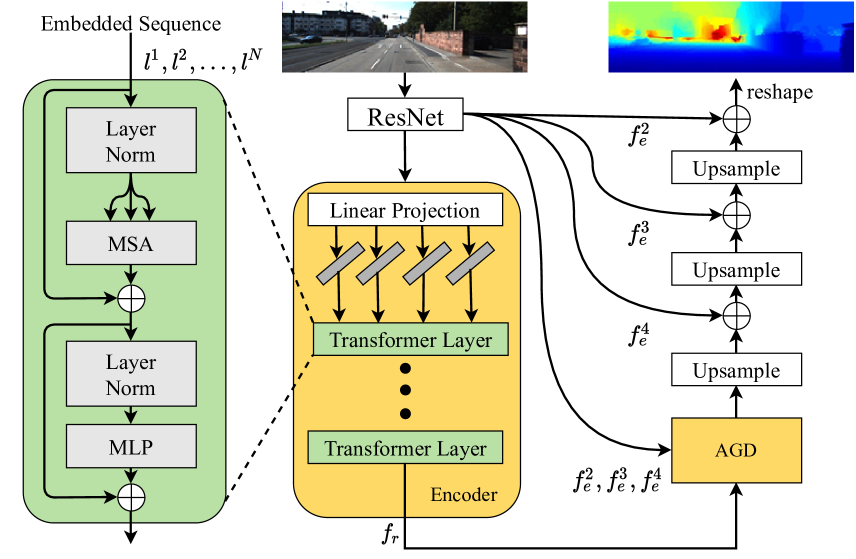
Figure 1: The overview of the proposed TransDepth. The symbols ⓒ and $\oplus$ denote concatenation and addition operations, respectively. AG is short for attention gate.

Our method focuses on representation learning as well but with only one step training strategy. The Transformer mechanism is quite suitable to solve the limited receptive field issue, to guide the generation of depth features. Unlike the previous works [72, 16] reshaping the image into a sequence of flattened 2D patches, we propose a hybrid model combining ResNet [27] and linear Transformer [16]. This is quite different from the previous Transformer mechanism, taking advantage of both sides. This composite structure also holds another advantage: many deep representation learning methods can be easily transferred in this network.

Surface Normal Estimation. Surface normal prediction is regarded as a close task to monocular depth prediction. Extracting 3D geometry from a single image has been a longstanding problem in computer vision. Surface normal estimation is a classical task in this context requiring modeling both global and local features. Typical approaches leverage networks with high capacity to achieve accurate predictions at high resolution. For instance, FrameNet [29] employed the DORN [20] architecture, a modification of DeepLabv3 [5] that removes multiple spatial reductions (2$\times$2 max pool layers), to generate high resolution surface normal maps. A different strategy consists of designing appropriate loss terms. For instance, UprightNet [62] considered an angular loss and showed its effectiveness for the task. More recently, Do et al. [15] proposed a novel truncated angular loss and a tilted image process, keeping the atrous spatial pyramid pooling (ASPP) module to increase the receptive field. Although its performance is SOTA, two extra training phases are added due to the tilted image process.

Attention Models. Several works have considered integrating attention models within deep architectures to improve performance in several tasks, such as image categorization [63], image generation [50, 49, 51, 52], video generation [40], speech recognition [9], and machine translation [54]. Focusing on pixel-level prediction, Chen et al.  [6] were the first to describe an attention model to combine multi-scale features learned by a FCN for semantic segmentation. Zhang et al. [70] designed EncNet, a network equipped with a channel attention mechanism to model the global context. Huang et al. [30] described CCNet, a deep architecture that embeds a criss-cross attention module with the idea of modeling contextual dependencies using sparsely connected graphs to achieve higher computational efficiency. Fu et al. [21] proposed to model semantic dependencies associated with spatial and channel dimensions by using two separate attention modules.

Our work significantly departs from these approaches as we introduce a novel attention gate mechanism, adding spatial- and channel-level attention into the attention decoder. Notably, we also prove that our model can be successfully employed in the case of several challenging dense continual pixel-level prediction tasks, where it significantly outperforms PGA-Net [64].

3 The Proposed TransDepth

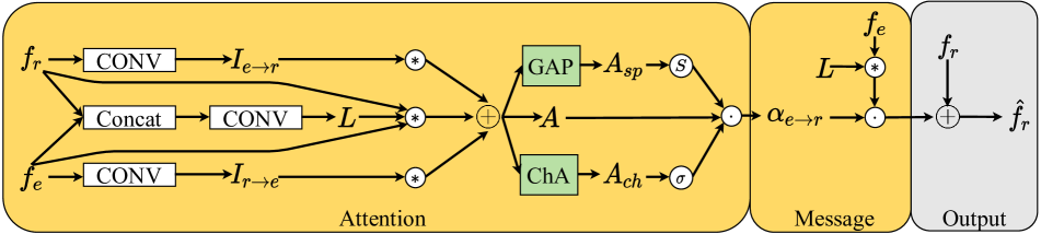
Figure 2: The overview of the proposed attention gate module. The symbols $\odot$, $\oplus$, $\sigma$⃝, $\ast$⃝, and \tiny{S}⃝ denote element-wise multiplication, element-wise addition, sigmoid, convolution, and softmax operation, respectively.

As previously discussed, our work aims to solve limited receptive fields by adding Transformer layers and enhancing the learned representation by an attention gate decoder.

3.1 Transformer for Depth Prediction

An overview of the network is depicted in Figure 1. Unlike the previous works [72, 4, 16] reshaping the image $I{\in}\mathbb{R}^{H\times W\times 3}$ into a sequence of flattened 2D patches $I_{p}{\in}\mathbb{R}^{N\times(p^{2}\cdot 3)}$, we propose a hybrid model. As shown in Figure 1, the input sequence comes from a ResNet backbone [27]. Then the patch embedding is applied to patches extracted from the final feature output of a CNN. This patch embedding’s kernel size should be $p{\times}p$, which means that the input sequence is obtained by simply flattening the spatial dimensions of the feature map and projecting to the Transformer dimension. In this case, we also remove position embedding because the original physical meaning is missing while mapping the vectorized patches $I_{p}$ into a latent embedding space $l_{p}$ using a linear projection. The input of the first Transformer layer is calculated as follow:

$$z_{0}=[l^{1}E;l^{2}E;\cdots;l^{N}E],$$ (1)

where $z_{0}$ is mapped into a latent N-dimensional embedding space using a trainable linear projection layer and $E$ is the patch embedding projection. There are $L$ Transformer layers which consist of multi-headed self-attention (MSA) and multi-layer perceptron (MLP) blocks. At each layer $\ell$, the input of the self-attention block is a triplet of $Q$ (query), $K$ (key), and $V$ (value), similar with [54], computed from $z_{\ell-1}{\in}\mathbb{R}^{L\times C}$ as:

$$Q=z_{\ell-1}\times W_{Q},K=z_{\ell-1}\times W_{K},V=z_{\ell-1}\times W_{V},$$ (2)

where $W_{Q},W_{K},W_{V}{\in}\mathbb{R}^{C\times d}$ are the learnable parameters of weight matrices and $d$ is the dimension of $Q$, $K$, $V$. The self-attention is calculated as:

$${\rm AH}={\rm softmax}(\frac{Q\times K^{T}}{\sqrt{d}})\cdot V,$$ (3)

where AH is short for attention head and $d$ is the dimension of self-attention block. MSA means the attention head will be calculated $m$ times by independent weight matrices. The final ${\rm MSA}(z_{\ell-1})$ is defined as:

$${\rm MSA}(z_{\ell-1})=z_{\ell-1}+{\rm concat}({\rm AH}_{1};{\rm AH}_{2};\cdots;{\rm AH}_{m})\times W_{o},$$ (4)

where $W_{o}{\in}\mathbb{R}^{md\times C}$. The output of ${\rm MSA}$ is then transformed by a MLP block with residual skip as the layer output as:

$$z_{\ell}={\rm MLP}({\rm LN}(z^{\prime}_{\ell}))+z^{\prime}_{\ell},$$ (5)

where ${\rm LN}(\cdot)$ means the layer normalization operator and $z^{\prime}_{\ell}{=}{\rm MSA}(z_{\ell-1})$. The structure of a Transformer layer is illustrated in the left part of Figure 1. After the Transformer layer, the output will be recovered to the original feature shape.

3.2 Attention Gate Decoder

Given an input image $\mathbf{I}$ and a generic front-end CNN model, we consider a set of $S$ multi-scale feature maps $\mathbf{F}{=}\{f^{i}\}_{i=1}^{N}$. Being a generic framework, these feature maps can be the output of $S$ intermediate CNN layers or of another representation, thus $s$ is a virtual scale. Opposite to previous works adopting simple concatenation or weighted averaging schemes [72], we propose to combine the multi-scale feature maps by learning a set of latent kernels ($I_{r\to e}$, $I_{e\to r}$, $L$) with a novel structure Attention-Gated module sketched in Figure 2. We choose $f^{N}$ as a receive feature only, $f_{r}$, while $\{f^{i}\}_{i=1}^{N-1}$ are chosen as emitting features, $f_{e}$, in all tasks. The influence of the fusion of different scales is explained in the ablation part.

In detail, the whole attention gate can be divided into two parts, i.e., attention and message. We propose to bring together recent advances in pixel-wise prediction by formulating a novel attention gate mechanism for the attention part. Inspired by [21], where two spatial- and channel-wise predictions are computed, we opt to infer different spatial and channel attention variables. Our attention tensor can be defined by:

$$A_{sp}^{i} =\frac{1}{C}\sum_{c=1}^{C}(\omega_{sp}*A^{i})[c,h,w],$$ (6)

$$A_{ch}^{i} =\frac{1}{HW}\sum_{h,w=1}^{H,W}(\omega_{sp}*A^{i})[c,h,w],$$

$$\alpha_{e\to r}^{i} ={\rm softmax}(A_{sp}^{i})\cdot\sigma(A_{ch}^{i})\cdot A^{i},$$

where $i$ means $f^{i}$ is chosen as an emitting feature. Different from [21], we adapt a local conditional kernel before generating attention. The kernels $I_{r\to e}$, $I_{e\to r}$, and $L$ are predicted from the input features using a linear transformation as follows:

$$\mathbf{L}^{i,j} ={\mathbf{W}_{L}}^{i,j}\mathrm{concat}(f_{e}^{i},f_{r}^{j})+{\mathbf{b}_{L}}^{i,j},$$ (7)

$$\mathbf{I}_{r\to e}^{i,j} ={\mathbf{W}_{I}}_{r\to e}^{i,j}\ f_{e}^{i}+{\mathbf{b}_{I}}_{r\to e}^{i,j},$$

$$\mathbf{I}_{e\to r}^{i,j} ={\mathbf{W}_{I}}_{e\to r}^{i,j}f_{r}^{j}+{\mathbf{b}_{I}}_{e\to r}^{i,j}.$$

Then, the integrated attention is defined as follow:

$$A^{i}=\mathbf{I}_{e\to r}^{i}*f_{r}+\mathbf{I}_{r\to e}^{i}*f_{e}^{i}+f_{r}*L*f_{e}^{i}.$$ (8)

Compared with the attention part, the message is easy to be calculated by $L^{i}*f_{r}$. Finally, the output of our attention gate decoder is:

$$\hat{f}_{e}^{i}={\rm concat}(L^{1}*f_{e}^{1}\cdot\alpha_{e\to r}^{1}+f_{r},...,L^{N-1}*f_{e}^{N-1}\cdot\alpha_{e\to r}^{N-1}+f_{r}).$$ (9)

Once the hidden variables are updated, we use them to address several different discrete prediction tasks, including monocular depth estimation and surface normal estimation. Following previous works, the network optimization loss for depth prediction, updated from [18], is:

$$\mathcal{L}_{depth}=\alpha\sqrt{\frac{1}{T}\sum_{i}g_{i}^{2}-\frac{\lambda}{T^{2}}(\sum_{i}g_{i})^{2}},$$ (10)

where $g_{i}{=}\log\hat{d}_{i}{-}\log d_{i}$ with the ground truth depth $d_{i}$ and the predicted depth $\hat{d}_{i}$. We set $\lambda$ and $\alpha$ to 0.85 and 10, same with [35]. The angular loss is chosen as the surface normal loss.

4 Experiments

4.1 Datasets

The NYU dataset [47] is used to evaluate our approach in the depth estimation task. We use 120K RGB-Depth pairs with a resolution of $480{\times}640$ pixels, acquired with a Microsoft Kinect device from 464 indoor scenes. We follow the standard train/test split as in [18], using 249 scenes for training and 215 scenes (654 images) for testing. We also use this dataset to evaluate our approach in the surface normal task, including 795 training images and 654 testing images.

The KITTI dataset [22] is a large-scale outdoor dataset created for various autonomous driving tasks. We use it to evaluate the depth estimation performance of our proposed model. Following the standard training/testing split proposed by Eigen et al. [18], we specifically use 22,600 frames from 32 scenes for training and 697 frames from the rest 29 scenes for testing.

The ScanNet dataset [11] is a large RGB-D dataset for 3D scene understanding. We employ it to evaluate the surface normal performance of our proposed model. ScanNet dataset is divided into 189,916 for training and 20,942 for testing with file lists provided in [11].

4.2 Evaluation Metrics

Evaluation Protocol on Monocular Depth Estimation. We follow the standard evaluation protocol as in previous works [17, 18, 57] and adopt the following quantitative evaluation metrics in our experiments:

• Abs relative error (abs-rel): $\frac{1}{K}\sum_{i=1}^{K}\frac{|\tilde{d}_{i}-d_{i}^{\star}|}{d_{i}^{\star}}$;

• Squared Relative difference (sq-rel): $\frac{1}{K}\sum_{i=1}^{K}\frac{||\tilde{d}_{i}-d_{i}^{\star}||^{2}}{d_{i}^{\star}}$;

• Root mean squared error (rms): $\sqrt{\frac{1}{K}\sum_{i=1}^{K}(\tilde{d}_{i}-d_{i}^{\star})^{2}}$;

• Mean log10 error (log-rms): $\sqrt{\frac{1}{K}\sum_{i=1}^{K}\|\log_{10}(\tilde{d}_{i})-\log_{10}(d_{i}^{\star})\|^{2}}$;

• Accuracy with threshold $t$: percentage (%) of $d_{i}^{\star}$, subject to $\max(\frac{d_{i}^{\star}}{\tilde{d}_{i}},\frac{\tilde{d}_{i}}{d_{i}^{\star}}){=}\delta{<}t~{}(t{\in}[1.25,1.25^{2},1.25^{3}])$;

where $\tilde{d}_{i}$ and $d_{i}^{\star}$ is the ground-truth depth and the estimated depth at pixel $i$ respectively; $K$ is the total number of pixels of the test images.

Evaluation Protocol on Surface Normal Estimation. We utilize five standard evaluation metrics [19]. For space limitation, we pick up median angle distance between prediction and ground-truth for valid pixels and the fraction of pixels with angle difference with ground-truth less than $11.25^{\circ}$ listed in the main paper. The results of five standard evaluation metrics are put into supplementary material.

4.3 Implementation Details

The proposed TransDepth is implemented in PyTorch. The experiments are conducted on four Nvidia Tesla V100 GPUs, each with 32 GB memory. The ResNet-50 architecture pretrained on ImageNet [13] is considered in the experiments for initializing the backbone network of our encoder network. For parameters of Transformer, T-layers, Hidden size, and attention multi-head are set to 12, 768, and 12, respectively. As the attention gate decoder structure setting, $f^{5}$ is chosen as the receiving feature, $f_{r}$, while $\{f^{i}\}_{i=3}^{5}$ are taken up as emitting features, $f_{e}$, in all tasks.

For the monocular depth estimation and surface normal prediction tasks, the learning rate is set to $10^{-4}$ with a weight decay of 0.01. The Adam optimizer is used in all our experiments with a batch size of 16 for all tasks. The total training epochs are set to 50 for depth prediction and 20 for surface normal prediction. We train our network on a random crop of size 352$\times$704 for KITTI dataset, 416$\times$512 for NYU dataset for depth prediction while the input image size is uniformly set to 320$\times$256 for surface normal prediction.

(a) Image

(b) GT

(c) FAL-Net

(d) Baseline

(e) Baseline w/ AGD

(f) Baseline w/ ViT

(g) Ours (Full)

Figure 3: Qualitative examples on the KITTI dataset.

Table 1: Depth Estimation: KITTI dataset. K: KITTI. CS: CityScapes [10]. CS$\to$K: CS pre-training. D: Depth supervision. M, Se, V, S: Monocular, segmentation, video, stereo. Sup: supervise.

Method	Sup	Data	Error (lower is better)				Accuracy (higher is better)
			abs rel	sq rel	rms	log rms	$\delta\textless 1.25$	$\delta\textless 1.25^{2}$	$\delta\textless 1.25^{3}$
CC [44]	M+Se	K	0.140	1.070	5.326	0.217	0.826	0.941	0.975
Bian et al. [2]	M+V	K+CS	0.137	1.089	5.439	0.217	0.830	0.942	0.975
DeFeat [48]	M	K	0.126	0.925	5.035	0.200	0.862	0.954	0.980
$S^{3}$Net [8]	M+Se	K	0.124	0.826	4.981	0.200	0.846	0.955	0.982
Monodepth2 [23]	M	K	0.115	0.903	4.863	0.193	0.877	0.959	0.981
pRGBD [53]	M	K	0.113	0.793	4.655	0.188	0.874	0.960	0.983
Johnston et al. [32]	M	K	0.106	0.861	4.699	0.185	0.889	0.962	0.982
SGDepth [33]	M+Se	K+CS	0.107	0.768	4.468	0.180	0.891	0.963	0.982
Shu et al. [46]	M	K	0.104	0.729	4.481	0.179	0.893	0.965	0.984
DORN [20]	D	K	0.072	0.307	2.727	0.120	0.932	0.984	0.994
Yin et al. [69]	M	K	0.072	-	3.258	0.117	0.938	0.990	0.998
PackNet [25]	V	K+CS	0.071	0.359	3.153	0.109	0.944	0.990	0.997
FAL-Net [24]	S	K+CS	0.068	0.276	2.906	0.106	0.944	0.991	0.998
PGA-Net [64]	D	K	0.063	0.267	2.634	0.101	0.952	0.992	0.998
BTS [35]	M	K	0.061	0.261	2.834	0.099	0.954	0.992	0.998
Baseline	M	K	0.106	0.753	3.981	0.104	0.888	0.967	0.986
Ours w/ AGD	M	K	0.065	0.261	2.766	0.101	0.953	0.993	0.998
Ours w/ ViT	M	K	0.064	0.258	2.761	0.099	0.955	0.993	0.999
Ours w/ AGD+ViT (Full)	M	K	0.064	0.252	2.755	0.098	0.956	0.994	0.999

4.4 Results on Monocular Depth Estimation

We compare the proposed method with the leading monocular depth estimation models, i.e., [44, 2, 48, 8, 23, 53, 32, 33, 46, 25, 20, 69, 24, 35]. Comparison results on the KITTI dataset are shown in Table 1. Our method performs favorably versus all previous fully- and self-supervised methods, achieving the best results on the majority of the metrics. Our approach employs the supervised setting using single monocular images in the training and testing phase. Compared with recent SOTA, i.e., FAL-Net, BTS, and PGA-Net, our method is better by a large margin. Meanwhile, unlike FAL-Net using stereo split, two-step training, and post-processing, our method is end-to-end without extra post-processing. The more important thing is that “Ours w/ ViT” has outperformed the SOTA. It can support our standpoint that adding a linear Transformer makes networks improve their ability to capture long-range dependencies. In other words, our network becomes more straightforward but more potent by adapting the linear Transformer.

(a) Image

(b) GT

(c) DORN

(d) BTS

(e) Ours

Figure 4: Qualitative examples on the NYU depth dataset.

Table 2: Depth Estimation: NYU dataset.

Method	Error (lower is better)			Accuracy (higher is better)
	rel	log10	rms	$\delta\textless 1.25$	$\delta\textless 1.25^{2}$	$\delta\textless 1.25^{3}$
PAD-Net [65]	0.214	0.091	0.792	0.643	0.902	0.977
Li et al. [38]	0.152	0.064	0.611	0.789	0.955	0.988
CLIFFNet [56]	0.128	0.171	0.493	0.844	0.964	0.991
Laina et al. [34]	0.127	0.055	0.573	0.811	0.953	0.988
MS-CRF [66]	0.121	0.052	0.586	0.811	0.954	0.987
Lee et al. [36]	0.119	0.050	-	0.870	0.974	0.993
Xia et al. [61]	0.116	-	0.512	0.861	0.969	0.991
DORN [20]	0.115	0.051	0.509	0.828	0.965	0.992
BTS [35]	0.113	0.049	0.407	0.871	0.977	0.995
Yin et al. [69]	0.108	0.048	0.416	0.875	0.976	0.994
Huynh et al. [31]	0.108	-	0.412	0.882	0.980	0.996
Baseline	0.118	0.051	0.414	0.866	0.979	0.995
Ours w/ AGD	0.111	0.048	0.393	0.881	0.979	0.996
Ours w/ ViT	0.109	0.047	0.388	0.887	0.981	0.996
Ours w/ AGD+ ViT (Full)	0.106	0.045	0.365	0.900	0.983	0.996

To demonstrate the competitiveness of our approach in an indoor scenario, we also evaluate the proposed method on the NYU depth dataset. The results are shown in Table 2, compared with the the state-of-the-art methods like [65, 38, 56, 34, 66, 36, 61, 20, 35, 69, 31]. Similar to the experiments on KITTI, it outperforms both state-of-the-art approaches and previous methods based on attention mechanism [66, 65, 31]. Our method successfully improves $\delta\textless 1.25$ from 0.882 (Huynh et al. [31]) to 0.900 while root mean squared error significantly drops to 0.365. Both Table 1 and  2 also show that our AGD can merge more low-level information and can make the network learn a more efficient deep representation. Moreover, Figure 3 shows a qualitative comparison of our method with DORN [20]. The red box marks the significant improvement parts. Results indicate that our method generates more precise boundaries for distant stuff like vehicles and traffic signs and near stuff like humans. Figure 4 shows a similar comparison done on the NYU dataset. Owing to applying the Transformer, the corners of the room are more distinguishable. This can support our standpoint that adapting the linear Transformer makes the CNN backbone network enhance the ability to capture long-range dependencies.

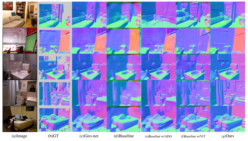
Figure 5: Qualitative examples on the NYU surface normal dataset.

Table 3: Surface Normal Estimation: NYU dataset.

Method	Training Data	Testing Data	median $\downarrow$	$11.25^{\circ}\uparrow$
Li et al. [37]	NYU	NYU	27.8	19.6
Chen et al. [7]			15.8	39.2
Eigen et al. [17]			13.2	44.4
SURGE [58]			12.2	47.3
Bansal et al. [1]			12.0	47.9
GeoNet [43]			12.5	46.0
TransDepth (Ours)			11.8	48.2
FrameNet [29]	ScanNet		11.0	50.7
VPLNet [59]			9.8	54.3
Do et al. [15]			8.1	59.8
TransDepth (Ours)			7.8	61.7

4.5 Results on Surface Normal Estimation

To prove our method universality, we also conduct experiments on surface normal prediction, which is regarded as a related task to depth prediction. We compare the proposed TransDepth with several state-of-the-art methods on surface normal, including GeoNet [43], VPLNet [59], FrameNet [29], and Do et al. [15]. For a fair comparison, we report our result in two different training conditions. Because of limited space, only median angle and $11.25^{\circ}$ are compared in Table 3 while a detailed comparison is shown in the supplementary. Our method outperforms the state-of-the-art on the median angle and $11.25^{\circ}$. Though Do et al. reduces the median angle error much, their method needs to get extra gravity labels with two-step pre-training. Our method covers these drawbacks. The qualitative results are shown in Figure 5. Unsurprisingly, the boundaries of stuff become more precise when AGD and ViT are jointly using.

4.6 Ablation Study

Effect of Attention Gate Decoder. We perform an ablation study on the NYU depth dataset to further demonstrate the impact of the proposed AGD. In Table 4, we indicate the emitting features in the $f_{e}$ column while we design $f_{5}$, the last layer’s output as the only receiving feature in all the experiments. We choose the ResNet-50 with the same prediction head as our baseline. We report four different combinations with the baseline when ViT is not applied to any candidates. Interestingly, the performance does not always get better by adding more scale information. In detail, the performance increases significantly with the emitting feature increasing until the number of emitting features reaches three. Compared with the last two rows in Table 4, some metrics like rel and rms go worse when the number of emitting features further expands. This could be explained by the fact that too many scale features may lead to overfitting the receiving feature. Undoubtedly, we choose three scales of fusion in all tasks. According to Figure 6, the attention granted by different scales fusion can capture information at different range distances. This can prove that the attention gate decoder is helpful to the receive feature to capture more position information.

Table 4: Ablation study on the NYU depth dataset: performance of TransDepth for different scales fusion.

		Error (lower is better)			Accuracy (higher is better)
$f_{e}$	$f_{r}$	rel	log10	rms	$\delta\textless 1.25$	$\delta\textless 1.25^{2}$	$\delta\textless 1.25^{3}$
-	-	0.118	0.051	0.414	0.866	0.979	0.995
$f^{5}$	$f^{5}$	0.120	0.071	0.407	0.878	0.982	0.996
$f^{4},f^{5}$	$f^{5}$	0.108	0.045	0.366	0.897	0.982	0.996
$f^{3},f^{4},f^{5}$	$f^{5}$	0.106	0.045	0.365	0.900	0.983	0.996
$f^{2},f^{3},f^{4},f^{5}$	$f^{5}$	0.107	0.045	0.366	0.899	0.983	0.996

Table 5: Ablation study about different backbone on the NYU depth dataset. R50 is short for ResNet50. B is short for base.

Backbone	Error (lower is better)			Accuracy (higher is better)
	rel	log10	rms	$\delta\textless 1.25$	$\delta\textless 1.25^{2}$	$\delta\textless 1.25^{3}$
ViT-B/32 [16]	0.112	0.048	0.387	0.849	0.927	0.940
ViT-B/16 [16]	0.108	0.046	0.371	0.885	0.967	0.979
ResNet50 [27]	0.118	0.051	0.414	0.866	0.979	0.995
ResNet101 [27]	0.112	0.048	0.387	0.848	0.927	0.939
ResNet152 [27]	0.111	0.047	0.381	0.861	0.941	0.953
R50+ViT-B/32	0.107	0.045	0.368	0.893	0.975	0.988
R50+ViT-B/16 (Ours)	0.106	0.045	0.365	0.900	0.983	0.996

Effect of Different Backbones. We also compare different backbones on the NYU depth dataset on Table 5 while the attention gate decoder is not used in this experiment. The 16/32 are no longer the input path size but the shrinkage scale of the input feature. In other words, 16 means the $f^{4}$ is the input feature of ViT-B, while 32 represents the $f^{5}$ is the input feature of ViT-B. Table 5 can be split into three-part: the top part belongs to the pure Transformer backbone; the middle part belongs to the pure ResNet backbone; the bottom belongs to the mixed backbone. Compared with the middle part results, the mixed backbone overpasses all of the pure ResNet backbones, leaving a significant margin for each metric. Meanwhile, according to Table 5, the mixed backbone is better than the ResNet backbone, and it outperforms the pure Transformer encoder. We finally pick up the ResNet-50 with ViT-B/16 as our network’s encoder for every task.

Figure 6: Qualitative attention examples of monocular depth prediction on the NYU dataset. The first column is the original image and the following three columns are different fusion attention.

5 Conclusions

We propose a novel Transformer-based framework, i.e., TransDepth, for the pixel-wise prediction problems involving continuous labels. We are the first to propose using Transformer to solve continuous pixel-wise prediction problems to the best of our knowledge. The proposed TransDepth leverages the inductive bias of ResNet on modeling spatial correlation and the powerful capability of Transformers on modeling global relationships. Moreover, a new and effective unified attention gate structure with independent channel-wise and spatial-wise attention is applied in the decoder. This can merge more low-level information and can make the network learn a more efficient deep representation. Extensive experiments prove that the proposed TransDepth establishes new state-of-the-art results on KITTI ($0.956$ on $\delta\textless 1.25$), NYU depth ($0.900$ on $\delta\textless 1.25$), and NYU surface normal ($61.7$ on $11.25^{\circ}$) datasets. We hope that this work can bring a new perspective on using Transformer-based architectures for computer vision tasks.

References

- [1] Aayush Bansal, Bryan Russell, and Abhinav Gupta. Marr revisited: 2d-3d alignment via surface normal prediction. In CVPR, 2016.
- [2] Jiawang Bian, Zhichao Li, Naiyan Wang, Huangying Zhan, Chunhua Shen, Ming-Ming Cheng, and Ian Reid. Unsupervised scale-consistent depth and ego-motion learning from monocular video. In NeurIPS, 2019.
- [3] Nicolas Carion, Francisco Massa, Gabriel Synnaeve, Nicolas Usunier, Alexander Kirillov, and Sergey Zagoruyko. End-to-end object detection with transformers. In ECCV, 2020.
- [4] Jieneng Chen, Yongyi Lu, Qihang Yu, Xiangde Luo, Ehsan Adeli, Yan Wang, Le Lu, Alan L Yuille, and Yuyin Zhou. Transunet: Transformers make strong encoders for medical image segmentation. arXiv, 2021.
- [5] Liang-Chieh Chen, George Papandreou, Iasonas Kokkinos, Kevin Murphy, and Alan L Yuille. Deeplab: Semantic image segmentation with deep convolutional nets, atrous convolution, and fully connected crfs. TPAMI, 2017.
- [6] Liang-Chieh Chen, Yi Yang, Jiang Wang, Wei Xu, and Alan L Yuille. Attention to scale: Scale-aware semantic image segmentation. In CVPR, 2016.
- [7] Weifeng Chen, Donglai Xiang, and Jia Deng. Surface normals in the wild. In ICCV, 2017.
- [8] Bin Cheng, Inderjot Singh Saggu, Raunak Shah, Gaurav Bansal, and Dinesh Bharadia. net: Semantic-aware self-supervised depth estimation with monocular videos and synthetic data. In ECCV, 2020.
- [9] Jan K Chorowski, Dzmitry Bahdanau, Dmitriy Serdyuk, Kyunghyun Cho, and Yoshua Bengio. Attention-based models for speech recognition. In NeurIPS, 2015.
- [10] Marius Cordts, Mohamed Omran, Sebastian Ramos, Timo Rehfeld, Markus Enzweiler, Rodrigo Benenson, Uwe Franke, Stefan Roth, and Bernt Schiele. The cityscapes dataset for semantic urban scene understanding. In CVPR, 2016.
- [11] Angela Dai, Angel X Chang, Manolis Savva, Maciej Halber, Thomas Funkhouser, and Matthias Nießner. Scannet: Richly-annotated 3d reconstructions of indoor scenes. In CVPR, 2017.
- [12] Zihang Dai, Zhilin Yang, Yiming Yang, Jaime Carbonell, Quoc V Le, and Ruslan Salakhutdinov. Transformer-xl: Attentive language models beyond a fixed-length context. ACL, 2019.
- [13] Jia Deng, Wei Dong, Richard Socher, Li-Jia Li, Kai Li, and Li Fei-Fei. Imagenet: A large-scale hierarchical image database. In CVPR, 2009.
- [14] Lei Ding, Dong Lin, Shaofu Lin, Jing Zhang, Xiaojie Cui, Yuebin Wang, Hao Tang, and Lorenzo Bruzzone. Looking outside the window: Wider-context transformer for the semantic segmentation of high-resolution remote sensing images. arXiv, 2021.
- [15] Tien Do, Khiem Vuong, Stergios I Roumeliotis, and Hyun Soo Park. Surface normal estimation of tilted images via spatial rectifier. In ECCV, 2020.
- [16] Alexey Dosovitskiy, Lucas Beyer, Alexander Kolesnikov, Dirk Weissenborn, Xiaohua Zhai, Thomas Unterthiner, Mostafa Dehghani, Matthias Minderer, Georg Heigold, Sylvain Gelly, et al. An image is worth 16x16 words: Transformers for image recognition at scale. In ICLR, 2021.
- [17] David Eigen and Rob Fergus. Predicting depth, surface normals and semantic labels with a common multi-scale convolutional architecture. In ICCV, 2015.
- [18] David Eigen, Christian Puhrsch, and Rob Fergus. Depth map prediction from a single image using a multi-scale deep network. In NeurIPS, 2014.
- [19] David F Fouhey, Abhinav Gupta, and Martial Hebert. Data-driven 3d primitives for single image understanding. In ICCV, 2013.
- [20] Huan Fu, Mingming Gong, Chaohui Wang, Kayhan Batmanghelich, and Dacheng Tao. Deep ordinal regression network for monocular depth estimation. In CVPR, 2018.
- [21] Jun Fu, Jing Liu, Haijie Tian, Yong Li, Yongjun Bao, Zhiwei Fang, and Hanqing Lu. Dual attention network for scene segmentation. In CVPR, 2019.
- [22] Andreas Geiger, Philip Lenz, Christoph Stiller, and Raquel Urtasun. Vision meets robotics: The kitti dataset. IJRR, 2013.
- [23] Clément Godard, Oisin Mac Aodha, Michael Firman, and Gabriel J Brostow. Digging into self-supervised monocular depth estimation. In ICCV, 2019.
- [24] Juan Luis Gonzalez and Munchurl Kim. Forget about the lidar: Self-supervised depth estimators with med probability volumes. In NeurIPS, 2020.
- [25] Vitor Guizilini, Rares Ambrus, Sudeep Pillai, Allan Raventos, and Adrien Gaidon. 3d packing for self-supervised monocular depth estimation. In CVPR, 2020.
- [26] Vitor Guizilini, Rui Hou, Jie Li, Rares Ambrus, and Adrien Gaidon. Semantically-guided representation learning for self-supervised monocular depth. In ICLR, 2020.
- [27] Kaiming He, Xiangyu Zhang, Shaoqing Ren, and Jian Sun. Deep residual learning for image recognition. In CVPR, 2016.
- [28] Han Hu, Zheng Zhang, Zhenda Xie, and Stephen Lin. Local relation networks for image recognition. In ICCV, 2019.
- [29] Jingwei Huang, Yichao Zhou, Thomas Funkhouser, and Leonidas J Guibas. Framenet: Learning local canonical frames of 3d surfaces from a single rgb image. In ICCV, 2019.
- [30] Zilong Huang, Xinggang Wang, Lichao Huang, Chang Huang, Yunchao Wei, and Wenyu Liu. Ccnet: Criss-cross attention for semantic segmentation. In ICCV, 2019.
- [31] Lam Huynh, Phong Nguyen-Ha, Jiri Matas, Esa Rahtu, and Janne Heikkilä. Guiding monocular depth estimation using depth-attention volume. In ECCV, 2020.
- [32] Adrian Johnston and Gustavo Carneiro. Self-supervised monocular trained depth estimation using self-attention and discrete disparity volume. In CVPR, 2020.
- [33] Marvin Klingner, Jan-Aike Termöhlen, Jonas Mikolajczyk, and Tim Fingscheidt. Self-supervised monocular depth estimation: Solving the dynamic object problem by semantic guidance. In ECCV, 2020.
- [34] Iro Laina, Christian Rupprecht, Vasileios Belagiannis, Federico Tombari, and Nassir Navab. Deeper depth prediction with fully convolutional residual networks. In 3DV, 2016.
- [35] Jin Han Lee, Myung-Kyu Han, Dong Wook Ko, and Il Hong Suh. From big to small: Multi-scale local planar guidance for monocular depth estimation. arXiv, 2019.
- [36] Jae-Han Lee and Chang-Su Kim. Multi-loss rebalancing algorithm for monocular depth estimation. In ECCV, 2020.
- [37] Bo Li, Chunhua Shen, Yuchao Dai, Anton Van Den Hengel, and Mingyi He. Depth and surface normal estimation from monocular images using regression on deep features and hierarchical crfs. In CVPR, 2015.
- [38] Jun Li, Reinhard Klein, and Angela Yao. A two-streamed network for estimating fine-scaled depth maps from single rgb images. In ICCV, 2017.
- [39] Fayao Liu, Chunhua Shen, and Guosheng Lin. Deep convolutional neural fields for depth estimation from a single image. In CVPR, 2015.
- [40] Gaowen Liu, Hao Tang, Hugo Latapie, Jason Corso, and Yan Yan. Cross-view exocentric to egocentric video synthesis. In ACM MM, 2021.
- [41] Ruijin Liu, Zejian Yuan, Tie Liu, and Zhiliang Xiong. End-to-end lane shape prediction with transformers. In WACV, 2021.
- [42] Chao Peng, Xiangyu Zhang, Gang Yu, Guiming Luo, and Jian Sun. Large kernel matters–improve semantic segmentation by global convolutional network. In CVPR, 2017.
- [43] Xiaojuan Qi, Renjie Liao, Zhengzhe Liu, Raquel Urtasun, and Jiaya Jia. Geonet: Geometric neural network for joint depth and surface normal estimation. In CVPR, 2018.
- [44] Anurag Ranjan, Varun Jampani, Lukas Balles, Kihwan Kim, Deqing Sun, Jonas Wulff, and Michael J Black. Competitive collaboration: Joint unsupervised learning of depth, camera motion, optical flow and motion segmentation. In CVPR, 2019.
- [45] Bin Ren, Hao Tang, Fanyang Meng, Runwei Ding, Ling Shao, Philip HS Torr, and Nicu Sebe. Cloth interactive transformer for virtual try-on. arXiv, 2021.
- [46] Chang Shu, Kun Yu, Zhixiang Duan, and Kuiyuan Yang. Feature-metric loss for self-supervised learning of depth and egomotion. In ECCV, 2020.
- [47] Nathan Silberman, Derek Hoiem, Pushmeet Kohli, and Rob Fergus. Indoor segmentation and support inference from rgbd images. In ECCV, 2012.
- [48] Jaime Spencer, Richard Bowden, and Simon Hadfield. Defeat-net: General monocular depth via simultaneous unsupervised representation learning. In CVPR, 2020.
- [49] Hao Tang, Song Bai, and Nicu Sebe. Dual attention gans for semantic image synthesis. In ACM MM, 2020.
- [50] Hao Tang, Song Bai, Li Zhang, Philip HS Torr, and Nicu Sebe. Xinggan for person image generation. In ECCV, 2020.
- [51] Hao Tang, Dan Xu, Nicu Sebe, Yanzhi Wang, Jason J Corso, and Yan Yan. Multi-channel attention selection gan with cascaded semantic guidance for cross-view image translation. In CVPR, 2019.
- [52] Hao Tang, Dan Xu, Nicu Sebe, and Yan Yan. Attention-guided generative adversarial networks for unsupervised image-to-image translation. In IJCNN, 2019.
- [53] Lokender Tiwari, Pan Ji, Quoc-Huy Tran, Bingbing Zhuang, Saket Anand, and Manmohan Chandraker. Pseudo rgb-d for self-improving monocular slam and depth prediction. In ECCV, 2020.
- [54] Ashish Vaswani, Noam Shazeer, Niki Parmar, Jakob Uszkoreit, Llion Jones, Aidan N Gomez, Lukasz Kaiser, and Illia Polosukhin. Attention is all you need. In NeurIPS, 2017.
- [55] Huiyu Wang, Yukun Zhu, Bradley Green, Hartwig Adam, Alan Yuille, and Liang-Chieh Chen. Axial-deeplab: Stand-alone axial-attention for panoptic segmentation. In ECCV, 2020.
- [56] Lijun Wang, Jianming Zhang, Yifan Wang, Huchuan Lu, and Xiang Ruan. Cliffnet for monocular depth estimation with hierarchical embedding loss. In ECCV, 2020.
- [57] Peng Wang, Xiaohui Shen, Zhe Lin, Scott Cohen, Brian Price, and Alan Yuille. Towards unified depth and semantic prediction from a single image. In CVPR, 2015.
- [58] Peng Wang, Xiaohui Shen, Bryan Russell, Scott Cohen, Brian Price, and Alan Yuille. Surge: Surface regularized geometry estimation from a single image. In NeurIPS, 2016.
- [59] Rui Wang, David Geraghty, Kevin Matzen, Richard Szeliski, and Jan-Michael Frahm. Vplnet: Deep single view normal estimation with vanishing points and lines. In CVPR, 2020.
- [60] Xiaolong Wang, Ross Girshick, Abhinav Gupta, and Kaiming He. Non-local neural networks. In CVPR, 2018.
- [61] Zhihao Xia, Patrick Sullivan, and Ayan Chakrabarti. Generating and exploiting probabilistic monocular depth estimates. In CVPR, 2020.
- [62] Wenqi Xian, Zhengqi Li, Matthew Fisher, Jonathan Eisenmann, Eli Shechtman, and Noah Snavely. Uprightnet: Geometry-aware camera orientation estimation from single images. In ICCV, 2019.
- [63] Tianjun Xiao, Yichong Xu, Kuiyuan Yang, Jiaxing Zhang, Yuxin Peng, and Zheng Zhang. The application of two-level attention models in deep convolutional neural network for fine-grained image classification. In CVPR, 2015.
- [64] Dan Xu, Xavier Alameda-Pineda, Wanli Ouyang, Elisa Ricci, Xiaogang Wang, and Nicu Sebe. Probabilistic graph attention network with conditional kernels for pixel-wise prediction. TPAMI, 2020.
- [65] Dan Xu, Wanli Ouyang, Xiaogang Wang, and Nicu Sebe. Pad-net: Multi-tasks guided prediction-and-distillation network for simultaneous depth estimation and scene parsing. In CVPR, 2018.
- [66] Dan Xu, Elisa Ricci, Wanli Ouyang, Xiaogang Wang, and Nicu Sebe. Multi-scale continuous crfs as sequential deep networks for monocular depth estimation. In CVPR, 2017.
- [67] Dan Xu, Wei Wang, Hao Tang, Hong Liu, Nicu Sebe, and Elisa Ricci. Structured attention guided convolutional neural fields for monocular depth estimation. In CVPR, 2018.
- [68] Guanglei Yang, Hao Tang, Zhun Zhong, Mingli Ding, Ling Shao, Nicu Sebe, and Elisa Ricci. Transformer-based source-free domain adaptation. arXiv, 2021.
- [69] Wei Yin, Yifan Liu, Chunhua Shen, and Youliang Yan. Enforcing geometric constraints of virtual normal for depth prediction. In ICCV, 2019.
- [70] Hang Zhang, Kristin Dana, Jianping Shi, Zhongyue Zhang, Xiaogang Wang, Ambrish Tyagi, and Amit Agrawal. Context encoding for semantic segmentation. In CVPR, 2018.
- [71] Hengshuang Zhao, Jianping Shi, Xiaojuan Qi, Xiaogang Wang, and Jiaya Jia. Pyramid scene parsing network. In CVPR, 2017.
- [72] Sixiao Zheng, Jiachen Lu, Hengshuang Zhao, Xiatian Zhu, Zekun Luo, Yabiao Wang, Yanwei Fu, Jianfeng Feng, Tao Xiang, Philip HS Torr, et al. Rethinking semantic segmentation from a sequence-to-sequence perspective with transformers. In CVPR, 2021.