Online learning with exponential weights in metric spaces

Abstract

This paper addresses the problem of online learning in metric spaces using exponential weights. We extend the analysis of the exponentially weighted average forecaster, traditionally studied in a Euclidean settings, to a more abstract framework. Our results rely on the notion of barycenters, a suitable version of Jensen’s inequality and a synthetic notion of lower curvature bound in metric spaces known as the measure contraction property. We also adapt the online-to-batch conversion principle to apply our results to a statistical learning framework.

1   Introduction

The problem of online convex optimization (Cesa-Bianchi and Lugosi, 2006, Shalev-Shwartz, 2012, Hazan, 2016) has become a strandard model of online learning. Its simple and flexible formulation as a repeated game, devoid of distributional assumptions on the data, has proven effective in framing theoretically a number of online prediction tasks including online recommendation systems, online portfolio selection or network routing problems. Traditionally studied in the context of Euclidean spaces, less seems to be known when the decision space is a more general metric space, with potentially no linear structure. In this paper, we extend the analysis of the exponentially weighted average (ewa) forecaster to some geodesic metric spaces.

Motivations for this level of generality arise, for example, when the decision space is a smooth manifold. Such a scenario is routinely encountered in directional or shape statistics (Mardia, 1999) where observations take values in spheres, projective spaces or shape spaces. Computer vision and medical imaging deal with spaces of transformations that carry a Lie group structure (Younes, 2019). The space of real symmetric positive-definite matrices with Bures metric (Bures, 1969), Log-Euclidean metric (Arsigny et al., 2007) or Log-Cholesky metric (Lin, 2019) have found important applications in quantum information theory or diffusion tensor imaging. Recent works have also demonstrated the use of hyperbolic spaces for applications in natural language processing (Nickel and Kiela, 2017). Other situations of interest involve spaces which cannot be endowed with a formal Riemannian structure such as the $2$-Wasserstein space (Villani, 2009, Santambrogio, 2015), the Billera-Holmes-Vogtmann space of phylogenetic trees (Billera et al., 2001) or the Gromov-Wasserstein space (Mémoli, 2011, Sturm, 2012). For a detailed survey on data analysis in non-standard spaces, we also refer the reader to Huckemann and Eltzner (2020).

All the spaces mentioned above share the characteristic of being geodesic spaces (Bridson and Haefliger, 1999, Burago et al., 2001, Alexander et al., 2019b, a), a structure that turns out to be rich enough to formulate and study the theoretical properties of a generalized version of the ewa forecaster, expanding the range of potential applications for online prediction strategies.

From a technical pespective, the definition of our learning strategy, called the exponentially weighted barycentric (ewb) forecaster, relies on the central notion of barycenters of probability measures. Its analysis is then based on an adapted version of Jensen’s inequality along with a general geometric property referred to as the measure contraction property that may be understood as a general definition of a lower Ricci curvature bound, in spaces that do not have a formal Riemannian structure.

The use the measure contraction property in the Euclidean setting, can be traced back to Blum and Kalai (1999) that use the scale invariance of the Lebesgue measure to analyse the performance of the universal rebalanced porfolio algorithm introduced by Cover (1991). Later, the same argument was leveraged by Hazan et al. (2007) to show that the ewa forecaster achieves logarithmic regret for general exponentially concave losses in Euclidean spaces. The argument we develop builds upon these original ideas, extending them to a more abstract framework.

The paper is organized as follows. Section 2 gathers basic definitions and necessary geometric background for our main results presented in Section 3. Proofs are reported to Section 4.

2   Preliminaries

2.1   Online optimization and the ewa forecaster

We first recall the protocol of online optimization as well as the construction of the classical ewa forecaster and refer the reader to Cesa-Bianchi and Lugosi (2006), Shalev-Shwartz (2012) or Hazan (2016) for more details.

Consider a decision space $M$ and a set $\mathcal{L}$ of loss functions $\ell:M\to\mathbb{R}$. At each round $t\geq 1$, a player has to choose to a point $x_{t}$ in $M$. After the player commits to their choice, the environment reveals a loss function $\ell_{t}\in\mathcal{L}$, the player incurs loss $\ell_{t}(x_{t})$ and moves on to round $t+1$. The goal of the player is to minimize their cumulative loss over time. A traditional performance measure after $n$ rounds of the game is the regret $R_{n}$ that compares the cumulative loss of the player to the cumulative loss of the best fixed point in hindsight, i.e.,

$$R_{n}=\sum_{t=1}^{n}\ell_{t}(x_{t})-\min_{x\in M}\sum_{t=1}^{n}\ell_{t}(x).$$

In this setting, the decision set $M$ is traditionally a convex subset of $\mathbb{R}^{p}$, for some $p\geq 1$, and a popular prediction strategy is given by the ewa forecaster defined as follows. First, let $m$ be a probability measure on the decision set $M$, encoding prior information. Then, given a sequence $(\beta_{t})_{t\geq 1}$ of positive tuning parameters, the ewa forecaster is defined, for all $t\geq 1$, by

$$x_{t}:=\int_{M}x\,\mathrm{d}m_{t}(x),$$ (2.1)

where $m_{1}:=m$ and, for all $t\geq 1$,

$$\mathrm{d}m_{t+1}(x):=\frac{e^{-\beta_{t+1}\ell_{t}(x)}}{\int_{M}e^{-\beta_{t+1}\ell_{t}}\,\mathrm{d}m_{t}}\,\mathrm{d}m_{t}(x).$$ (2.2)

This popular forecaster naturally emphasizes the role of points that exhibit a small cumulative loss over time and its analysis is simplified by the convenient properties of the exponential function. Since its introduction by Vovk (1990) and Littlestone and Warmuth (1994), the ewa forecaster has been analyzed in the Euclidean setting from many perspectives (see, e.g, Cesa-Bianchi and Lugosi, 1999, Blum and Kalai, 1999, Hazan et al., 2007). The use of exponential weights has also found many applications in Statistics in the context of aggregation (Yang, 2004, Leung and Barron, 2006, Catoni, 2007, Dalalyan and Tsybakov, 2007, 2008, 2009, Juditsky et al., 2008, Alquier, 2008, Audibert, 2009, Dalalyan and Tsybakov, 2012a, b).

In the Euclidean setting, the linear and convex structure of the decision space $M$ is important for several reasons. First, it allows to make sense of the integral defining $x_{t}$ in (2.1). Second, it is essential to the traditional notion of convexity of losses $\ell\in\mathcal{L}$ usually invoked in the analysis of $x_{t}$. As it turns out, a simple adaptation of the construction of $x_{t}$ given in (2.1), using the notion of barycenters, makes sense in an abstract metric space and reduces to the ewa forecaster in the Euclidean setting. The rest of this section reports some definitions and tools that will be used in the sequel to define and study this adaptation.

2.2   Geodesic spaces and convexity

Let $(M,d)$ be a metric space. For $\tau>0$, a path $\gamma:[0,\tau]\to M$ is called a geodesic if, for all $0\leq s\leq t\leq\tau$,

$$d(\gamma(s),\gamma(t))=\frac{t-s}{\tau}d(\gamma(0),\gamma(1)).$$ (2.3)

Geodesics can be equivalently defined as constant-speed reparametrizations of length minimizing paths for an appropriate notion of length in metric spaces.

Definition 2.1.

The space $(M,d)$ is called geodesic if, for every $x,y\in M$, there exists a geodesic $\gamma:[0,1]\to M$ connecting $x$ to $y$, i.e., such that $\gamma(0)=x$ and $\gamma(1)=y$.

Fundamental examples of geodesic spaces are complete and connected Riemannian manifolds equipped with the Riemannian distance (Bridson and Haefliger, 1999, Corollary 3.20). The class of geodesic spaces includes however many other examples and we refer the reader to Bridson and Haefliger (1999), Burago et al. (2001), Alexander et al. (2019b, a) for more details.

Definition 2.2.

Let $(M,d)$ be a geodesic space.

1. For $\alpha\in\mathbb{R}$, a function $f:M\to\mathbb{R}$ is called geodesically $\alpha$-convex if, for every geodesic $\gamma:[0,1]\to M$, the function

   $$t\in[0,1]\mapsto f(\gamma(t))-\frac{\alpha}{2}d^{2}(\gamma(0),\gamma(t)),$$

   is convex. We call $f$ geodesically convex if it is geodesically $0$-convex and geodesically concave if $-f$ is geodesically convex.

2. For $\beta>0$, a function $f:M\to\mathbb{R}$ is called geodesically $\beta$-expconcave if the function $\exp(-\beta f)$ is geodesically concave.

Lemma 2.3.

Let $(M,d)$ be a complete geodesic space and $f:M\to\mathbb{R}$ be a given function.

1. Suppose that $f$ is geodesically $\beta$-expconcave for some $\beta>0$. Then, the function $f$ is geodesically convex.

2. Suppose that $f$ is geodesically $\alpha$-convex and $L$-Lipchitz for some $\alpha,L>0$. Then, it is geodesically $\beta$-expconcave for all $0<\beta\leq\frac{\alpha}{L^{2}}$.

These definitions reduce to familiar notions of convexity in the context of Euclidean spaces. In particular, the second statement in Lemma 2.3 extends to geodesic spaces a classical result by Hazan et al. (2007) in the context of Euclidean spaces.

2.3   Alexandrov curvature bounds

For $\kappa\in\mathbb{R}$, a remarkable geodesic space is the $\kappa$-plane $(M^{2}_{\kappa},d_{\kappa})$ defined as the unique (up to isometry) $2$-dimensional, complete and simply connected, Riemannian manifold with constant sectional curvature $\kappa$, equipped with its Riemannian distance $d_{\kappa}$. The diameter $D_{\kappa}$ of $M^{2}_{\kappa}$ is

$$D_{\kappa}:=\left\{\begin{array}[]{cc}+\infty&\mbox{if}\quad\kappa\leq 0,\\ \pi/\sqrt{\kappa}&\mbox{if}\quad\kappa>0,\end{array}\right.$$

and there is a unique geodesic $[0,1]\to M$ connecting $x$ to $y$ in $M^{2}_{\kappa}$ provided $d_{\kappa}(x,y)<D_{\kappa}$.

Given a metric space $(M,d)$, we call triangle in $M$ any set of three points $\{p,x,y\}\subset M$. For $\kappa\in\mathbb{R}$, a comparison triangle for $\{p,x,y\}\subset M$ in $M^{2}_{\kappa}$ is an isometric copy $\{\bar{p},\bar{x},\bar{y}\}\subset M^{2}_{\kappa}$ of $\{p,x,y\}$ in $M^{2}_{\kappa}$ (i.e., pairwise distances are preserved). Such a comparison triangle always exists and is unique (up to an isometry) provided the perimeter $\mathrm{peri}\{p,x,y\}:=d(p,x)+d(p,y)+d(x,y)<2D_{\kappa}$.

Definition 2.4.

For $\kappa\in\mathbb{R}$, we say that a geodesic space $(M,d)$ has curvature bounded below by $\kappa$, and denote ${\rm curv}(M)\geq\kappa$, if for any triangle $\{p,x,y\}\subset M$ with $\mathrm{peri}\{p,x,y\}<2D_{\kappa}$ and any geodesic $\gamma:[0,1]\to M$ connecting $x$ to $y$ in $M$, we have

$$\forall t\in[0,1],\quad d(p,\gamma(t))\geq d_{\kappa}(\bar{p},\bar{\gamma}(t)),$$ (2.4)

where $\{\bar{p},\bar{x},\bar{y}\}$ is the unique comparison triangle of $\{p,x,y\}$ in $M^{2}_{\kappa}$ and where $\bar{\gamma}:[0,1]\to M^{2}_{\kappa}$ is any geodesic connecting $\bar{x}$ to $\bar{y}$ in $M^{2}_{\kappa}$. Similarly, we say that $M$ has curvature bounded above by $\kappa$, and denote ${\rm curv}(M)\leq\kappa$, if the same holds with opposite inequality in (2.4).

The $0$-plane $(M^{2}_{0},d_{0})$ is the familiar Euclidean plane. The properties of the Euclidean plane allow to reformulate, in simpler terms, the definition of curvature bounds in the case $\kappa=0$.

Corollary 2.5.

A geodesic space $(M,d)$ satisfies ${\rm curv}(M)\geq 0$ iff, for all $p,x,y\in M$, any geodesic $\gamma:[0,1]\to M$ connecting $x$ to $y$ in $M$, and any $t\in[0,1]$,

$$d^{2}(p,\gamma(t))\geq(1-t)d^{2}(p,x)+td^{2}(p,y)-t(1-t)d^{2}(x,y).$$ (2.5)

Similarly, ${\rm curv}(M)\leq 0$ if the same holds with opposite inequality in (2.5).

Combining Definition 2.2 and Corollary 2.5, it follows that ${\rm curv}(M)\leq 0$ iff, for all $p\in M$, the function $d^{2}(p,.):M\to\mathbb{R}_{+}$ is $2$-convex. In particular, we deduce directly from Lemma 2.3, and the triangular inequality, the following fact.

Corollary 2.6.

Let $(M,d)$ be a geodesic space satisfying ${\rm curv}(M)\leq 0$ and with finite diameter. Then, for all $p\in M$, the function $d^{2}(p,.):M\to\mathbb{R}_{+}$ is $\beta$-concave for all $0<\beta\leq 1/(2\,\mathrm{diam}(M)^{2})$.

Next is a list of (complete and separable) geodesic spaces that have curvature bounds in the sense of Definition 2.4.

Example 2.7.

1. A normed vector space $V$ has a curvature bound from above, or below, iff it is a pre-Hilbert space, in which case it satisfies ${\rm curv}(V)\geq 0$ and ${\rm curv}(V)\leq 0$ since (2.5) holds as an identity.

2. For any $\kappa\in\mathbb{R}$, a complete Riemannian manifold $M$ with sectional curvature everywhere lower bounded by $\kappa$ satisfies ${\rm curv}(M)\geq\kappa$.

3. For $\kappa\leq 0$, a complete and simply connected Riemannian manifold $M$ with sectional curvature everywhere upper bounded by $\kappa$ satisfies ${\rm curv}(M)\leq\kappa$.

4. The frontier $\partial K$ of a convex body $K\subset\mathbb{R}^{p}$ equipped with its length metric is a geodesic space satisfying $\mathrm{curv}(\partial K)\geq 0$.

5. A (complete and separable) geodesic space $(\Omega,d)$ satisfies $\mathrm{curv}(\Omega)\geq 0$ iff the space $\mathcal{P}_{2}(\Omega)$, equipped with the $2$-Wasserstein metric, satisfies $\mathrm{curv}(\mathcal{P}_{2}(\Omega))\geq 0$ (Sturm, 2006a, Proposition 2.10).

2.4   Barycenters and Jensen’s inequality

Given a metric space $(M,d)$, let $\mathcal{P}_{2}(M)$ be the set of Borel probability measures $m$ on $M$ satisfying, for all $x\in M$,

$$\mathcal{V}_{m}(x):=\int_{M}d^{2}(x,y)\,{\rm d}m(y)<+\infty.$$

For $m\in\mathcal{P}_{2}(M)$, we call $\mathcal{V}_{m}:M\to\mathbb{R}_{+}$ its variance functional and denote

$$\mathcal{V}^{*}_{m}:=\inf_{x\in M}\mathcal{V}_{m}(x).$$ (2.6)

Definition 2.8.

Given a metric space $(M,d)$ and $m\in\mathcal{P}_{2}(M)$, a barycenter of $m$ is any $x^{*}\in M$ such that

$$\mathcal{V}_{m}(x^{*})=\mathcal{V}^{*}_{m}.$$ (2.7)

Barycenters provide a generalization of the notion of mean value when $M$ has no linear structure. While alternative notions of mean value in a metric space have been proposed, barycenters are often favored for their simple interpretation and constructive definition as solution of an optimization problem. The question of existence and uniqueness of barycenters has been addressed in a number of settings. While uniqueness will be of less interest in the sequel, we mention two classical results on the existence of barycenters.

• If $M$ is geodesic and locally compact, then any $m\in\mathcal{P}_{2}(M)$ admits at least one barycenter.

• If $M$ is geodesic, complete and satisfies ${\rm curv}(M)\leq 0$, then any $m\in\mathcal{P}_{2}(M)$ admits a (unique) barycenter (Sturm, 2003, Theorem 4.9).

In specific geodesic spaces which do not necessarily satisfy these assumptions, the existence and uniqueness of barycenters can be obtained via a taylored analysis such as in Wasserstein spaces (see, e.g. Agueh and Carlier, 2011, Le Gouic and Loubes, 2017).

Along with the notion of barycenters, a fundamental result needed next is a suitable version of Jensen’s inequality. We mention two results in this direction.

Lemma 2.9 (Sturm, 2003, Theorem 6.2).

Let $(M,d)$ be a complete geodesic space with ${\rm curv}(M)\leq 0$. Let $m\in\mathcal{P}_{2}(M)$ and let $x^{*}$ be its unique barycenter. Let $f:M\to\mathbb{R}$ be convex and lower semi-continuous. Then we have

$$f(x^{*})\leq\int_{M}f\,\mathrm{d}m,$$

provided $f$ is either positive or in $L^{1}(m)$.

Lemma 2.10 (Paris, 2020, Theorem 1.1).

Let $(M,d)$ be a complete and separable geodesic space with ${\rm curv}(M)\geq\kappa$, for some $\kappa\in\mathbb{R}$. Let $m\in\mathcal{P}_{2}(M)$ and suppose that it admits at least one barycenter $x^{*}$. Let $f:M\to\mathbb{R}$ be $\alpha$-convex, for some $\alpha\in\mathbb{R}$, and Lipschitz in a neighborhood of $x^{*}$. Then we have

$$f(x^{*})\leq\int_{M}f\,\mathrm{d}m-\frac{\alpha}{2}\mathcal{V}^{*}_{m},$$

provided $f$ is either positive or in $L^{1}(m)$.

2.5   The measure contraction property

Curvature bounds in the sense of Alexandrov, defined in paragraph 2.3, generalize the notion of sectional curvature bounds of Riemannian manifolds (see statements $(2)$ and $(3)$ of Example 2.7). In this paragraph, we discuss the measure contraction property (mcp), which generalizes lower Ricci curvature bounds for Riemannian manifolds. In the recent years, a number of synthetic definitions of lower Ricci curvature bounds have been developed in the abstract context of metric-measure spaces (see, e.g., Sturm, 2006a, b, Ohta, 2007, Lott and Villani, 2009). These have shown to imply many of the analytical properties expected in the context of Riemannian manifolds, under a Ricci curvature lower bound, in a wider context. The mcp property defined below is known to be one of the weakest forms of such definitions (see Remark 2.15).

Consider a metric-measure space $(M,d,m)$ where $(M,d)$ is a complete and separable geodesic space and $m$ is a reference positive Borel measure on $M$. Suppose in addition that $0<m(B(x,r))<+\infty$ for all $x\in M$ and all $r>0$, where $B(x,r):=\{y\in M:d(x,y)<r\}$.

Definition 2.11.

Given $x\in M$, we call geodesic homothety of center $x$ any measurable map $h_{x}:M\times[0,1]\to M$ such that, for $m$-a.e. $y\in M$, the map $h_{x}(y,.):[0,1]\to M$ is a geodesic connecting $x$ to $y$.

A geodesic homothety is to be understood as a generalization of the map $h_{x}(y,\varepsilon):=(1-\varepsilon)x+\varepsilon y$, in a Euclidean space, contracting points towards the center $x$ with ratio $\varepsilon$. The mcp property defined next, quantifies the way Borel subsets of $M$ contract toward the center $x$ under the the action of $h_{x}$. For $\kappa\in\mathbb{R}$ and $r\geq 0$, we denote

$$s_{\kappa}(r):=\left\{\begin{array}[]{cc}\frac{\sin(r\sqrt{\kappa})}{\sqrt{\kappa}}&\mbox{if }\kappa>0,\\ r&\mbox{if }\kappa=0,\\ \frac{\sinh(r\sqrt{-\kappa})}{\sqrt{-\kappa}}&\mbox{if }\kappa<0.\end{array}\right.$$ (2.8)

Definition 2.12 (Ohta, 2007, Lemma 2.3).

For $\kappa\in\mathbb{R}$ and $p>1$, the space $(M,d,m)$ is said to satisfy the measure contraction property mcp$(\kappa,p)$ if, for all $x\in M$, there exists a geodesic homothety $h_{x}$ with center $x$ such that, for every measurable subset $A\subset M$ (with $A\subset B(x,\pi\sqrt{(p-1)/\kappa})$ if $\kappa>0$) and every $\varepsilon\in[0,1]$,

$$m(A^{\varepsilon}_{x})\geq\int_{A}\varepsilon\left(\frac{s_{\kappa}(\varepsilon d(x,y)/\sqrt{p-1})}{s_{\kappa}(d(x,y)/\sqrt{p-1})}\right)^{p-1}\,m(\mathrm{d}y),$$

where $A^{\varepsilon}_{x}:=\{h_{x}(y,\varepsilon):y\in A\}$ and with the convention $0/0=1$.

Example 2.13.

1. Suppose $M$ is a complete Riemannian manifold of dimension $p$. Let $d$ be the Riemannian distance and $m$ the volume measure. Then $\mathrm{Ric}_{M}\geq\kappa$ iff $(M,d,m)$ satisfies the mcp$(\kappa,p)$ property. In addition, for any function $f:M\to\mathbb{R}_{+}$ and any $q>0$ such that $f^{1/q}$ is geodesically concave, the weighted space $(M,d,fm)$ satisfies the mcp$(\kappa,p+q)$ property.  (Sturm, 2006b, Corollary 5.5(i)).

2. Let $(M,d)$ be a complete and locally compact geodesic space with curvature lower bounded by $\kappa\in\mathbb{R}$ in the sense of Definition 2.4 and finite Hausdorff dimension $p$. Then letting $m$ be the $p$-dimensional Hausdorff measure, $(M,d,m)$ satisfies the mcp$((p-1)\kappa,p)$ property (Kuwae and Shioya, 2010, Theorem 1.1).

Remark 2.14.

Given a metric measure space $(M,d,m)$ and $\alpha>0$, it appears clearly from the definition that $(M,d,m)$ satisfies the mcp$(\kappa,p)$ property if and only $(M,d,\alpha m)$ satisfies the same property. In particular, provided $0<m(M)<+\infty$, we can suppose that $m$ is a probability measure without loss of generality.

Remark 2.15.

An alternative, and more popular, synthetic definition of Ricci curvature lower bound is the curvature-dimension condition cd$(\kappa,p)$. Under minimal regularity conditions on the space $(M,d,m)$, this condition is known to imply the mcp$(\kappa,p)$ property (Sturm, 2006b, Theorem 5.4). Conversely, some examples of spaces satisfying the mcp property but not the cd property are known (see, e.g., Juillet, 2009, Rizzi, 2016).

3   Results

We adopt the same notation as in paragraph 2.1. We suppose that the decision set $(M,d)$ is a (complete and separable) geodesic space. We fix a prior distribution $m\in\mathcal{P}_{2}(M)$ and suppose that the following properties hold.

1. Existence of barycenters
   Any $\mu\in\mathcal{P}_{2}(M)$ admits at least one barycenter.

2. Jensen’s inequality
   For any $\mu\in\mathcal{P}_{2}(M)$, any barycenter $x^{*}$ of $\mu$ and any geodesically convex $f:M\to\mathbb{R}$, either positive or in $L^{1}(\mu)$, we have

   $$f(x^{*})\leq\int_{M}f\,{\rm d}\mu.$$

3. Measure contraction property
   There exists $\kappa\in\mathbb{R}$ and $p>1$ such that $(M,d,m)$ satisfies the mcp$(\kappa,p)$ property.

Note that Assumptions (A1) and (A2) refer to characteristics of the metric space $(M,d)$ while (A3) refers to a property of the metric-measure space $(M,d,m)$. It follows from section 2 that these properties are satisfied in a wide setting. For instance, typical examples for which all three assumptions are satisfied at once include:

• Bounded and locally compact geodesic spaces $(M,d)$ with finite Hausdorff dimension $p>1$, curvature lower bounded by $\kappa/(p-1)$ for some $\kappa\in\mathbb{R}$ in the sense of Definition 2.4 and equipped with the renormalized $p$-dimensional Hausdorff measure $m$.

• Complete and connected Riemannian manifolds of dimension $d<p$, with the Riemannian distance, sectional curvature lower bounded by $\kappa/(p-1)$ for some $\kappa\in\mathbb{R}$ (and hence $\mathrm{Ric}_{M}\geq\kappa$) and reference measure $m$ with density $f$ with respect to the volume measure such that $f^{1/(p-d)}$ is geodesically concave.

3.1   The ewb forecaster

We are now in position to define a learning strategy we call the Exponentially Weighted Barycentric (ewb) forecaster.

Definition 3.1.

Let $(\beta_{t})_{t\geq 1}$ be a sequence of positive tuning parameters. Then, for $t\geq 1$, we define $x_{t}$ as a barycenter of $m_{t}$, i.e.,

$$x_{t}\in\underset{x\in M}{\arg\min}\int_{M}d^{2}(x,y)\,m_{t}(\mathrm{d}y),$$ (3.1)

where, as in the classical setting, $m_{1}:=m$ and, for all $t\geq 1$,

$$\mathrm{d}m_{t+1}(x):=\frac{e^{-\beta_{t+1}\ell_{t}(x)}}{\int_{M}e^{-\beta_{t+1}\ell_{t}}\,\mathrm{d}m_{t}}\,\mathrm{d}m_{t}(x).$$

3.2   Regret bounds

Throughout the rest of the section, we denote

$$\psi(r):=(r\coth r)\exp(-r\coth r),$$

for $r>0$, set $\psi(0)=e^{-1}$ and define, for all $x\in M$, all $p>1$ and all $\kappa\in\mathbb{R}$,

$$c_{\kappa,p}(x):=\left\{\begin{array}[]{cc}1&\mbox{if }\kappa\geq 0,\\ \int_{M}\psi\left(d(x,y)\sqrt{\frac{-\kappa}{p-1}}\right)\,m(\mathrm{d}y)&\mbox{if }\kappa<0.\end{array}\right.$$

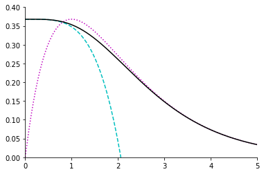
Figure 1: Plot of function $\psi(r)=(r\coth r)\exp(-r\coth r)$ (solid line), equivalent to $\psi_{0}(r)=1/e-r^{4}/18e$ (dashed line) at $0$ and to $\psi_{\infty}(r)=r\exp(-r)$ (dotted line) at $+\infty$.

Theorem 3.2.

Assume that (A1), (A2) and (A3) hold. Suppose that there exists $\beta>0$ such that every $\ell\in\mathcal{L}$ is geodesically $\beta$-expconcave. Then taking $\beta_{t}=\beta$ for all $t\geq 1$ and selecting any

$$x^{*}_{n}\in\underset{x\in M}{\arg\min}\,\sum_{t=1}^{n}\ell_{t}(x),$$ (3.2)

the regret of the ewb forecaster satisfies, for all $n\geq 2$,

$$R_{n}\leq\frac{1}{\beta}\left(2+\ln\frac{1}{c_{\kappa,p}(x^{*}_{n})}\right)+\frac{p\ln n}{\beta}.$$

When $\kappa\geq 0$, the regret bound displayed in Theorem 3.2 reads

$$R_{n}\leq\frac{2}{\beta}+\frac{p\ln n}{\beta}.$$

This regret bound was already obtained for the case where $M\subset\mathbb{R}^{p}$ is a bounded convex set, with non-empty interior, equipped with Euclidean metric and uniform measure (Hazan et al., 2007, Theorem 7). The above result shows that this behavior is exactly preserved whenever $(M,d,m)$ satisfies Assumptions (A1)-(A3) with $\kappa\geq 0$. In the case of $\kappa<0$, the regret bound displays the additional term

$$\frac{1}{\beta}\ln\frac{1}{c_{\kappa,p}(x^{*}_{n})}=\frac{1}{\beta}\ln\frac{1}{\int_{M}\psi\left(d(x^{*}_{n},y)\sqrt{\frac{-\kappa}{p-1}}\right)\,m(\mathrm{d}y)},$$

whose behavior, as $n$ goes to infinity, isn’t straightforward in full generality. Under the additional assumption that $M$ has bounded diameter, the monotonicity of function $\psi$, displayed in Figure 1, implies however that this additional term is upper bounded, independently of $n$, by

$$\frac{1}{\beta}\ln\frac{1}{\psi\left(\mathrm{diam}(M)\sqrt{\frac{-\kappa}{p-1}}\right)},$$

guaranteeing in this case also a regret of order at most $(p\ln n)/\beta$. In the case where $\kappa<0$ and $M$ isn’t bounded, an obvious restriction on $(M,d,m)$, allowing for a logarithmic regret, is to impose that

$$\inf_{x\in M}c_{\kappa,p}(x)=\inf_{x\in M}\int_{M}\psi\left(d(x,y)\sqrt{\frac{-\kappa}{p-1}}\right)\,m(\mathrm{d}y)>0.$$ (3.3)

Finally we note that, as in the Euclidean setting, an important aspect of the above regret bound is that it does not require the losses to be Lipschitz. As a remark, we show however that, at the price of this additional requirement, we can obtain a similar regret bound under a more general assumption.

Proposition 3.3.

Assume that (A1) and (A2) hold. Assume that there exists constants $p,r_{0}>0$ and a function $c:M\to\mathbb{R}_{+}$ such that

$$\forall x\in M,\forall r\in(0,r_{0}],\quad m(B(x,r))>c(x)r^{p}.$$ (3.4)

Assume finally that there exist $\beta,L>0$ such that every $\ell\in\mathcal{L}$ is geodesically $\beta$-expconcave and $L$-Lipschitz. Then taking $\beta_{t}=\beta$ for all $t\geq 1$, the regret of the ewb forecaster satisfies, for all $n\geq 1/r_{0}$,

$$R_{n}\leq L+\frac{1}{\beta}\ln\frac{1}{c(x^{*}_{n})}+\frac{p\ln n}{\beta},$$

for $x^{*}_{n}\in M$ as in (3.2).

We show next that property (3.4) is indeed more general than the measure contraction property.

Proposition 3.4.

Suppose that $(M,d,m)$ satisfies the measure contraction property mcp$(\kappa,p)$ for some $\kappa\in\mathbb{R}$ and some $p>1$. Then, there exists $p,r_{0}>0$ and $c:M\to\mathbb{R}_{+}$ such that property (3.4) holds.

We end the paragraph by mentioning results valid for bounded losses that are only geodesically convex. For brevity, the proof is reported in the Appendix.

Theorem 3.5.

Assume that (A1) and (A2) hold. Suppose that every $\ell\in\mathcal{L}$ is geodesically convex and $[a,b]$-valued. Then setting, for all $t\geq 1$,

$$\beta_{t}=\frac{2c_{1}}{(b-a)}\sqrt{\frac{\ln(t\lor 2)}{t}}\quad\mbox{where}\quad c_{1}:=\left(\frac{3}{2}\right)^{\frac{1}{4}}\leq 1.1,$$

the regret of the ewb forecaster satisfies the following.

1. If Assumption (A3) holds, then for all $n\geq 2$,

   $$\frac{R_{n}}{b-a}\leq 1+c_{1}\left(1+\ln\frac{1}{c_{\kappa,p}(x^{\star}_{n})}\right)\sqrt{pn\ln n},$$

   where $c_{\kappa,p}$ and $x^{*}_{n}$ are as in Theorem 3.2.

2. If more generally property (3.4) holds and all losses $\ell\in\mathcal{L}$ are also $L$-Lipschitz, then for all $n\geq 1/r_{0}$,

   $$\frac{R_{n}}{b-a}\leq\frac{L}{b-a}+c_{1}\left(1+\ln\frac{1}{c(x^{*}_{n})}\right)\sqrt{pn\ln n},$$

   for $x^{*}_{n}\in M$ as in (3.2).

3.3   Online to batch conversion

The principle of online-to-batch conversion is a classical way to exploit algorithms, developed for sequential prediction, in the context of statistical learning. This section presents a simple adaptation of this procedure in the context of metric spaces.

Consider the following statistical learning problem. Let $(M,d)$ be a metric space, let $\mathcal{Z}$ be an arbitrary measurable space and let $\ell:M\times\mathcal{Z}\to\mathbb{R}$ be a fixed loss function. Suppose given a collection (or batch) $\{Z_{i}\}_{i=1}^{n}$ of independent and identically distributed $\mathcal{Z}$-valued random variables with same distribution as (and independent from) a generic random variable $Z$. Finally, consider the task of constructing $\hat{\theta}_{n}\in M$ based on $\{Z_{i}\}_{i=1}^{n}$ and such that the excess risk

$$\mathbb{E}[\ell(\hat{\theta}_{n},Z)]-\inf_{\theta\in M}\mathbb{E}[\ell(\theta,Z)],$$

is as small as possible.

To that aim, consider first the problem of online optimization studied so far with decision space $M$ and loss functions $\mathcal{L}=\{\ell(.,z):z\in\mathcal{Z}\}$. In this setting, at each round $t\geq 1$ the player first chooses a point $\theta_{t}\in M$, the environment then reveals a point $z_{t}$, the player incurs loss $\ell(\theta_{t},z_{t})$ and moves on to round $t+1$. Here, the players strategy $(\theta_{t})_{t\geq 1}$ can be formally associated to a sequence of measurable maps $(\vartheta_{t})_{t\geq 1}$ where $\vartheta_{1}$ is constantly equal to $\theta_{1}$ and, for $t\geq 2$, $\vartheta_{t}:\mathcal{Z}^{t-1}\to M$ is such that

$$\theta_{t}=\vartheta_{t}(z_{1},\dots,z_{t-1}).$$

Now, suppose given such a prediction strategy $(\vartheta_{t})_{t\geq 1}$ and suppose that, for all $n\geq 1$, there exists $B_{n}>0$ satisfying

$$\sum_{t=1}^{n}\ell(\theta_{t},z_{t})-\inf_{\theta\in M}\sum_{t=1}^{n}\ell(\theta,z_{t})\leq B_{n},$$ (3.5)

uniformly over the outcome sequence $(z_{1},\dots,z_{n})\in\mathcal{Z}^{n}$.

Then, coming back to the statistical learning problem, consider $\hat{\theta}_{n}$ to be a barycenter of the (random) probability measure

$$\frac{1}{n+1}\delta_{\vartheta_{1}}+\frac{1}{n+1}\sum_{t=2}^{n+1}\delta_{\vartheta_{t}(Z_{1},\dots,Z_{t-1})},$$

on $M$, i.e.,

$$\hat{\theta}_{n}\in\underset{\theta\in M}{\arg\min}\left\{d^{2}(\theta,\vartheta_{1})+\sum_{t=2}^{n+1}d^{2}(\theta,\vartheta_{t}(Z_{1},\dots,Z_{t-1}))\right\}.$$ (3.6)

Then we have the following result.

Theorem 3.6.

Suppose that the metric space $(M,d)$ satisfies Assumptions (A1) and (A2). Suppose that (3.5) holds uniformly over the outcome sequence $(z_{1},\dots,z_{n})\in\mathcal{Z}^{n}$ and that, for all $z\in\mathcal{Z}$, the function $\ell(.,z):M\to\mathbb{R}$ is geodesically convex. Then, for all $n\geq 1$,

$$\mathbb{E}[\ell(\hat{\theta}_{n},Z)]-\inf_{\theta\in M}\mathbb{E}[\ell(\theta,Z)]\leq\frac{B_{n+1}}{n+1}.$$

Combining Theorems 3.2 and 3.6, we readily obtain the following result. A similar adaptation of Theorem 3.5 is left to the reader.

Corollary 3.7.

Suppose that $(M,d)$ satisfies Assumptions (A1) and (A2). Let $m$ be a prior distribution over $M$ such that $(M,d,m)$ satisfies Assumption (A3) and condition (3.3) if $\kappa<0$. Suppose that there exists $\beta>0$ such that, for all $z\in\mathcal{Z}$, the function $\ell(.,z):M\to\mathbb{R}$ is geodesically $\beta$-expconcave. Let $\hat{\theta}_{n}$ be as in (3.6) where $\vartheta_{1}$ is a barycenter of $m$ and, for $2\leq t\leq n+1$, $\vartheta_{t}(Z_{1},\dots,Z_{t-1})$ is a barycenter of the (random) probability measure $m_{t}$ defined by

$$\mathrm{d}m_{t}(\theta)=\frac{e^{-\beta\ell(\theta,Z_{t-1})}}{\int_{M}e^{-\beta\ell(.,Z_{t-1})}\mathrm{d}m_{t-1}}\mathrm{d}m_{t-1}(\theta),$$

where $m_{1}:=m$. Then, for all $n\geq 2$,

$$\mathbb{E}[\ell(\hat{\theta}_{n},Z)]-\inf_{\theta\in M}\mathbb{E}[\ell(\theta,Z)]\leq\frac{2+\ln(\inf_{M}c_{\kappa,p})^{-1}}{\beta(n+1)}+\frac{p\ln(n+1)}{\beta(n+1)}.$$

3.4   Example: The $2$-Wasserstein space over $\mathbb{R}^{d}$

Consider the set $\mathcal{P}_{2}(\mathbb{R}^{d})$ of all square integrable (Borel) probability measures over $\mathbb{R}^{d}$. Given $\mu,\nu\in\mathcal{P}_{2}(\mathbb{R}^{d})$, denote $\Pi_{\mu,\nu}$ the set of couplings between $\mu$ and $\nu$, i.e., the set of probability measures $\pi$ on $\mathbb{R}^{d}\times\mathbb{R}^{d}$ satisfying $\pi(.\times\mathbb{R}^{d})=\mu$ and $\pi(\mathbb{R}^{d}\times.)=\nu$. The $2$-Wasserstein metric $W_{2}$ on $\mathcal{P}_{2}(\mathbb{R}^{d})$ is defined by

$$W^{2}_{2}(\mu,\nu):=\inf_{\pi\in\Pi_{\mu,\nu}}\int_{\mathbb{R}^{d}\times\mathbb{R}^{d}}\|x-y\|^{2}_{2}\,{\rm d}\pi(x,y).$$

The metric space $(\mathcal{P}_{2}(\mathbb{R}^{d}),W_{2})$ is called the $2$-Wasserstein space over $\mathbb{R}^{d}$. It is complete, separable, geodesic and has non-negative curvature in the sense of Definition 2.4 (Sturm, 2006a, Proposition 2.10). The existence and uniqueness of barycenters of probability measures on $\mathcal{P}_{2}(\mathbb{R}^{d})$ have been established under general conditions. For instance Le Gouic and Loubes (2017) show that, for any $P\in\mathcal{P}_{2}(\mathcal{P}_{2}(\mathbb{R}^{d}))$,

• $P$ admits a barycenter,

• if there exists a Borel subset $B\subset\mathcal{P}_{2}(\mathbb{R}^{d})$ such that $P(B)>0$ and such that every $\mu\in B$ has a density with respect to the Lebesgue measure, then this barycenter is unique.

Assumptions (A1)-(A3) are therefore verified for a subset $M\subset\mathcal{P}_{2}(\mathbb{R}^{d})$ equipped with the Wasserstein metric provided the following conditions are satisfied:

1. $M$ is a geodesically convex subset of $\mathcal{P}_{2}(\mathbb{R}^{d})$ in the sense that for any $\mu,\nu\in M$ and any geodesic $\gamma:[0,1]\to\mathcal{P}_{2}(\mathbb{R}^{d})$ connecting $\mu$ to $\nu$, the image of $\gamma$ is included in $M$,

2. $M$ has finite Hausdorff dimension $p$

We end with a result of special interest for online learning with the $W_{2}$ loss in the $2$-Wasserstein space. Recall first that, according to the Kantorovich dual representation of $W_{2}$, for all $\mu,\nu\in\mathcal{P}_{2}(\mathbb{R}^{D})$,

$$W^{2}_{2}(\mu,\nu)=\sup_{\varphi}\int(\|.\|^{2}-2\varphi)\,{\rm d}\mu+\int(\|.\|^{2}-2\varphi^{*})\,{\rm d}\nu,$$

where $\varphi:\mathbb{R}^{D}\to\mathbb{R}\cup\{-\infty\}$ ranges over the set of proper and lower semi-continuous convex functions and $\varphi^{*}$ denotes the Fenchel-Legendre conjugate of $\varphi$. In addition, the supremum is always attained and a $\varphi_{\mu\to\nu}$ achieving the max is called an optimal Kantorovich potential.

Lemma 3.8.

Let $P\in\mathcal{P}_{2}(\mathcal{P}_{2}(\mathbb{R}^{D}))$ and suppose $\Delta:=\mathrm{diam}(\mathrm{supp}(P))<+\infty$. Let $\mu^{*}$ be a barycenter of $P$ and suppose that, for $P$-almost all $\nu$, $\varphi_{\mu^{*}\to\nu}$ is $\alpha(\nu)$-strongly convex for a measurable $\alpha:\mathcal{P}_{2}(\mathbb{R}^{D})\to\mathbb{R}_{+}$. Then $\mu^{*}$ is unique and, for all $\mu$ in the support of $P$, and all

$$0<\beta\leq\frac{8\mathcal{V}^{*}_{P}}{\Delta^{4}},$$

we have

$$W^{2}_{2}(\mu^{*},\mu)\leq-\frac{C^{-1}_{\rm var}}{\beta}\ln\int\exp(-\beta W^{2}_{2}(\mu,.))\,\mathrm{d}P,$$ (3.7)

where $C_{\rm var}:=\int\alpha(\nu){\rm d}P(\nu)$.

4   Proofs

4.1   Proof of Lemma 2.3

$(1)$ Suppose that $f$ is $\beta$-expconcave for some $\beta>0$. Then, since the logarithm is increasing and concave, we get that, for any geodesic $\gamma:[0,1]\to M$ and all $t\in[0,1]$,

$$f(\gamma_{t}) =-\frac{1}{\beta}\ln e^{-\beta f(\gamma_{t})}$$

$$\leq-\frac{1}{\beta}\ln((1-t)e^{-\beta f(\gamma_{0})}+te^{-\beta f(\gamma_{1})})$$

$$\leq(1-t)f(\gamma_{0})+tf(\gamma_{1}).$$

$(2)$ Suppose $f:M\to\mathbb{R}$ is geodesically $\alpha$-convex and $L$-Lipchitz for some $\alpha,L>0$. Using the fact that $M$ is complete, it is enough to show that for every $0\leq\beta\leq\alpha/L^{2}$ and every geodesic $\gamma:[0,1]\to M$, we have

$$\frac{1}{2}e^{-\beta f(\gamma_{0})}+\frac{1}{2}e^{-\beta f(\gamma_{1})}\leq e^{-\beta f(\gamma_{1/2})},$$

or, equivalently, that

$$\frac{1}{2}e^{\beta(f(z)-f(x))}+\frac{1}{2}e^{\beta(f(z)-f(y))}\leq 1,$$ (4.1)

where $x=\gamma_{0},y=\gamma_{1}$ and $z=\gamma_{1/2}$. By $\alpha$-convexity of $f$, we have that

$$f(z)\leq\frac{1}{2}f(x)+\frac{1}{2}f(y)-\frac{\alpha}{8}d(x,y)^{2},$$

so that

$$\beta(f(z)-f(x))\leq\frac{\beta}{2}(f(y)-f(x))-\frac{\alpha\beta}{8}d(x,y)^{2},$$

and

$$\beta(f(z)-f(y))\leq\frac{\beta}{2}(f(x)-f(y))-\frac{\alpha\beta}{8}d(x,y)^{2}.$$

For (4.1) to be satisfied, it is therefore enough to have

$$\frac{1}{2}e^{\frac{\beta}{2}(f(y)-f(x))}+\frac{1}{2}e^{\frac{\beta}{2}(f(x)-f(y))}=\cosh(\frac{\beta}{2}(f(x)-f(y)))\leq e^{\frac{\alpha\beta}{8}d(x,y)^{2}}.$$

Now, using the fact that $\cosh(u)\leq e^{\frac{u^{2}}{2}}$ for all $u\in\mathbb{R}$, the Lipschitz assumption implies that

$$\cosh(\frac{\beta}{2}(f(x)-f(y)))\leq e^{\frac{\beta^{2}L^{2}}{8}d(x,y)^{2}}.$$

As a result, it is enough to have $\beta^{2}L^{2}\leq\alpha\beta$, i.e., $\beta\leq\alpha/L^{2}$, as required.

4.2   Proof of Theorem 3.2

We start with three preliminary results. The first lemma below follows the lines devised in Gyorfi and Ottucsak (2007) and is reported for completeness.

Lemma 4.1.

Provided $0<\beta_{t+1}\leq\beta_{t}$, for all $t\geq 1$, we have for all $n\geq 1$,

$$-\sum_{t=1}^{n}\frac{1}{\beta_{t}}\ln\left(\int_{M}e^{-\beta_{t}\ell_{t}}\,\mathrm{d}m_{t}\right)\leq-\frac{1}{\beta_{n+1}}\ln\left(\int_{M}e^{-\beta_{n+1}L_{n}}\,\mathrm{d}m\right),$$ (4.2)

where $L_{n}:=\sum_{t=1}^{n}\ell_{t}$.

Proof of Lemma 4.1.

For all $t\geq 1$, denote

$$W_{t}:=\int_{M}e^{-\beta_{t}L_{t-1}}\,\mathrm{d}m,$$

with the convention that $L_{0}(x)=0$, for all $x\in M$. Since $W_{1}=1$ we get

$$\frac{\ln W_{n+1}}{\beta_{n+1}} =\sum_{t=1}^{n}\left(\frac{\ln W_{t+1}}{\beta_{t+1}}-\frac{\ln W_{t}}{\beta_{t}}\right)$$

$$=\sum_{t=1}^{n}\left(\frac{\ln W_{t+1}}{\beta_{t+1}}-\frac{\ln W^{*}_{t+1}}{\beta_{t}}\right)+\sum_{t=1}^{n}\frac{1}{\beta_{t}}\ln\left(\frac{W^{*}_{t+1}}{W_{t}}\right),$$ (4.3)

where

$$W^{*}_{t+1}:=\int_{M}e^{-\beta_{t}L_{t}}\,\mathrm{d}m.$$

Since $0<\beta_{t+1}\leq\beta_{t}$, Jensen’s inequality implies that

$$W_{t+1}=\int_{M}e^{-\beta_{t+1}L_{t}}\,\mathrm{d}m\leq\left(\int_{M}e^{-\beta_{t}L_{t}}\,\mathrm{d}m\right)^{\frac{\beta_{t+1}}{\beta_{t}}}=(W^{*}_{t+1})^{\frac{\beta_{t+1}}{\beta_{t}}},$$

which shows that the first sum in expression (4.3) is non-positive. Hence, we get

$$\frac{\ln W_{n+1}}{\beta_{n+1}} \leq\sum_{t=1}^{n}\frac{1}{\beta_{t}}\ln\left(\frac{W^{*}_{t+1}}{W_{t}}\right)$$

$$=\sum_{t=1}^{n}\frac{1}{\beta_{t}}\ln\int_{M}e^{-\beta_{t}\ell_{t}}\,\mathrm{d}m_{t},$$

which concludes the proof. ∎

The next Lemma is also known in the Euclidean context but holds in our setting. Below, we denote $\mathcal{E}(\mu|m)$ the relative entropy of $\mu$ with respect to $m$, i.e.,

$$\mathcal{E}(\mu|m):=\int_{M}\ln\left(\frac{{\rm d}\mu}{{\rm d}m}\right){\rm d}\mu,$$

if $\mu\ll m$, and $\mathcal{E}(\mu|m):=+\infty$ otherwise.

Lemma 4.2.

Assume that (A1) and (A2) hold. Suppose that there exists $\beta>0$ such that every $\ell\in\mathcal{L}$ is geodesically $\beta$-expconcave. Then the cumulative loss of the ewb forecaster, with $\beta_{t}=\beta$ for all $t\geq 1$, satisfies

$$\sum_{t=1}^{n}\ell_{t}(x_{t})\leq\inf_{\mu}\left\{\int_{M}L_{n}\,\mathrm{d}\mu+\frac{\mathcal{E}(\mu|m)}{\beta}\right\},$$

where $L_{n}:=\sum_{t=1}^{n}\ell_{t}$ and where the inf runs over all probability measures $\mu$ on $M$.

Proof of Lemma 4.2.

By concavity of $\exp(-\beta\ell_{t})$, Assumption (A2) implies that

$$\ell_{t}(x_{t})\leq-\frac{1}{\beta}\ln\int_{M}e^{-\beta\ell_{t}}\mathrm{d}m_{t}.$$

Summing over $1\leq t\leq n$ and using Lemma 4.1, it follows that

$$\sum_{t=1}^{n}\ell_{t}(x_{t})\leq-\frac{1}{\beta}\ln\left(\int_{M}e^{-\beta L_{n}}\,\mathrm{d}m\right).$$

It remains to observe that, according to the Gibbs variational principle, we have

$$-\frac{1}{\beta}\ln\left(\int_{M}e^{-\beta L_{n}}\,\mathrm{d}m\right)=\inf_{\mu}\left\{\int_{M}L_{n}\,\mathrm{d}\mu+\frac{\mathrm{Ent}(\mu|m)}{\beta}\right\}.$$

∎

Lemma 4.3.

1. For all $0\leq r\leq\pi$ and all $\varepsilon\in(0,1)$,

   $$\frac{\sin(\varepsilon r)}{\sin(r)}\geq\varepsilon,$$

   with the convention $0/0=1$.

2. For all $r\geq 0$ and all $\varepsilon\in(0,1/2]$,

   $$\frac{\sinh(\varepsilon r)}{\sinh(r)}\geq\varepsilon\psi(r),$$

   with $\psi(r):=(r\coth r)\exp(-r\coth r)$ and the convention $0/0=1$.

Proof of Lemma 4.3.

$(1)$ The statement follows from the concavity of the sine function on $[0,\pi]$. $(2)$ A direct computation shows that, for any $r>0$, the map $g:(0,1]\to\mathbb{R}$ defined by

$$g(\varepsilon):=\log\sinh(\varepsilon r),$$

is concave. Hence, for all $\varepsilon\in(0,1]$, we have

$$g(\varepsilon)-g(1)\geq-(1-\varepsilon)g^{\prime}(\varepsilon)=-\varepsilon(1-\varepsilon)f(r)\geq-\varepsilon f(r),$$

where we denote $f(r):=r\coth r$. Therefore, since $1+x\leq e^{x}$ for $x\geq 0$, it follows that

$$\frac{\sinh(\varepsilon r)}{\sinh(r)} =\exp(g(\varepsilon)-g(1))$$

$$\geq\exp(-\varepsilon f(r))$$

$$=\exp((1-\varepsilon)f(r))\exp(-f(r))$$

$$\geq(1+(1-\varepsilon)f(r))\exp(-f(r))$$

$$\geq\varepsilon f(r)\exp(-f(r)),$$

where the last inequality uses the fact that $\varepsilon\leq 1/2$. ∎

Proof of Theorem 3.2.

Fix $n\geq 2$ and

$$x^{*}_{n}\in\underset{x\in M}{\arg\min}\,L_{n}(x).$$

Let $h:M\times[0,1]\to M$ be a geodesic homothety with center $x^{*}_{n}$ for which the measure contraction property (A3) holds. For $\varepsilon\in(0,1)$, denote

$$M_{\varepsilon}:=M^{\varepsilon}_{x^{*}_{n}}=\{h(y,\varepsilon):y\in M\},$$

and introduce the probability measure

$$m_{\varepsilon}(.):=\frac{m(.\cap M_{\varepsilon})}{m(M_{\varepsilon})}.$$

According to Lemma 4.2 we deduce that

$$\sum_{t=1}^{n}\ell_{t}(x_{t}) \leq\int_{M}L_{n}\mathrm{d}m_{\varepsilon}+\frac{\mathcal{E}(m_{\varepsilon}|m)}{\beta}$$

$$=\frac{1}{m(M_{\varepsilon})}\int_{M_{\varepsilon}}L_{n}\mathrm{d}m+\frac{1}{\beta}\ln\left(\frac{1}{m(M_{\varepsilon})}\right).$$ (4.4)

Then, since $h(y,.):[0,1]\to M$ is a geodesic connecting $x^{*}_{n}$ to $y$, the $\beta$-expconcavity of the losses implies that

$$e^{-\beta\ell_{t}(h(y,\varepsilon))}\geq(1-\varepsilon)e^{-\beta\ell_{t}(x^{*}_{n})}+\varepsilon e^{-\beta\ell_{t}(y)}\geq(1-\varepsilon)e^{-\beta\ell_{t}(x^{*}_{n})},$$

and therefore

$$e^{-\beta L_{n}(h(y,\varepsilon))}\geq(1-\varepsilon)^{n}e^{-\beta L_{n}(x^{*}_{n})},$$

which implies

$$L_{n}(h(y,\varepsilon))\leq\frac{n}{\beta}\ln\left(\frac{1}{1-\varepsilon}\right)+L_{n}(x^{*}_{n}).$$

Combining this inequality with (4.4), we obtain

$$R_{n}\leq\frac{n}{\beta}\ln\left(\frac{1}{1-\varepsilon}\right)+\frac{1}{\beta}\ln\left(\frac{1}{m(M_{\varepsilon})}\right).$$

It remains to bound $m(M_{\varepsilon})$ from below. According to (A3) we have

$$m(M_{\varepsilon})\geq\int_{M}\varepsilon\left(\frac{s_{\kappa}(\varepsilon d(x^{*}_{n},y)/\sqrt{p-1})}{s_{\kappa}(d(x^{*}_{n},y)/\sqrt{p-1})}\right)^{p-1}\,m(\mathrm{d}y).$$

To make this lower bound more explicit, we consider three cases.

$\bullet$ Suppose $\kappa>0$. Then, according to the Bonnet-Myers Theorem, valid under the mcp property (Ohta, 2007, Theorem 4.3), the diameter of $M$ is at most $\pi\sqrt{(p-1)/\kappa}$. Hence, it follows from Lemma 4.3 point $(1)$, and the definition of $s_{\kappa}$ in display (2.8), that for all $\varepsilon\in(0,1)$, $m(M_{\varepsilon})\geq\varepsilon^{p}$ which implies that

$$R_{n}\leq\frac{n}{\beta}\ln\left(\frac{1}{1-\varepsilon}\right)+\frac{p}{\beta}\ln\frac{1}{\varepsilon}.$$

Taking $\varepsilon=1/n$, and using the standard inequality $\ln(1+x)\leq x$, we obtain in particular

$$R_{n}\leq\frac{n}{\beta}\ln\left(\frac{n}{n-1}\right)+\frac{p\ln n}{\beta}\leq\frac{n}{\beta(n-1)}+\frac{p\ln n}{\beta},$$

as desired.

$\bullet$ Suppose $\kappa=0$. Then since $s_{\kappa}(r)=r$, the mcp property reads in this case $m(M_{\varepsilon})\geq\varepsilon^{p}$ and we conclude as above.

$\bullet$ Suppose $\kappa<0$. Then Lemma 4.2 point $(2)$ implies that, for all $\varepsilon\in(0,1/2]$

$$m(M_{\varepsilon}) \geq\varepsilon^{p}\int_{M}\psi\left(d(x^{*}_{n},y)\sqrt{\frac{-\kappa}{p-1}}\right)\,m(\mathrm{d}y)$$

$$=c_{\kappa,p}(x^{*}_{n})\varepsilon^{p}.$$

Hence, for all $\varepsilon\in(0,1/2]$,

$$R_{n}\leq\frac{n}{\beta}\ln\left(\frac{1}{1-\varepsilon}\right)+\frac{1}{\beta}\ln\frac{1}{c_{\kappa,p}(x^{*}_{n})}+\frac{p}{\beta}\ln\frac{1}{\varepsilon}.$$

Hence taking $\varepsilon=1/n$ allows to conclude as in the previous cases. ∎

4.3   Proof of Proposition 3.3

Consider

$$x^{*}_{n}\in\underset{x\in M}{\arg\min}\,L_{n}(x).$$

For $r\in(0,r_{0}]$, define the probability measure

$$\mu_{r}(.):=\frac{m(.\cap B(x^{*}_{n},r))}{m(B(x^{*}_{n},r))}.$$

According to Lemma 4.2 we deduce that

$$\sum_{t=1}^{n}\ell_{t}(x_{t}) \leq\int_{M}L_{n}\mathrm{d}\mu_{r}+\frac{\mathcal{E}(\mu_{r}|m)}{\beta}$$

$$=\frac{1}{m(B(x^{*}_{n},r))}\int_{B(x^{*}_{n},r)}L_{n}\mathrm{d}m+\frac{1}{\beta}\ln\left(\frac{1}{m(B(x^{*}_{n},r))}\right)$$

$$\leq\frac{1}{m(B(x^{*}_{n},r))}\int_{B(x^{*}_{n},r)}L_{n}\mathrm{d}m+\frac{1}{\beta}\ln\frac{1}{c(x^{*}_{n})}+\frac{p}{\beta}\ln\frac{1}{r},$$

by Assumption (3.4). Substracting $L_{n}(x^{*}_{n})$ on both sides and using the Lipschitz property of the losses, we obtain, for all $r\in(0,r_{0}]$,

$$R_{n} \leq nLr+\frac{1}{\beta}\ln\frac{1}{c(x^{*}_{n})}+\frac{p}{\beta}\ln\frac{1}{r}.$$

Taking finally $r=1/n$ implies the desired result.

4.4   Proof of Proposition 3.4

According to Ohta (2007, Lemma 2.5), for all $0<r\leq r_{0}$ (and $r_{0}\leq\pi\sqrt{(p-1)/\kappa}$ if $\kappa>0$), we have, for all $x\in M$,

$$\frac{m(B(x,r))}{m(B(x,r_{0}))}\geq\frac{r}{r_{0}}\inf_{\varepsilon\in[0,1]}\left(\frac{s_{\kappa}(\varepsilon r/\sqrt{p-1})}{s_{\kappa}(\varepsilon r_{0}/\sqrt{p-1})}\right)^{p-1}.$$

In particular, for all $0<r\leq r_{0}$ (and $2r_{0}\leq\pi\sqrt{(p-1)/\kappa}$ if $\kappa>0$), Lemma 4.3 and the fact that the map $\psi(u)=(u\coth u)\exp(-u\coth u)$ is decreasing on $\mathbb{R}_{+}$ (see Figure 1), we obtain

$$\inf_{\varepsilon\in[0,1]}\left(\frac{s_{\kappa}(\varepsilon r/\sqrt{p-1})}{s_{\kappa}(\varepsilon 2r_{0}/\sqrt{p-1})}\right)^{p-1}\geq c(\kappa,p,r_{0})\left(\frac{r}{2r_{0}}\right)^{p-1},$$

where constant $c(\kappa,p,r_{0})=1$ if $\kappa\geq 0$ and

$$c(\kappa,p,r_{0}):=\psi\left(2r_{0}\sqrt{\frac{-\kappa}{p-1}}\right)^{p-1},$$

if $\kappa<0$. In particular, for all $0<r\leq r_{0}$ (and $2r_{0}\leq\pi\sqrt{(p-1)/\kappa}$ if $\kappa>0$), we obtain

$$m(B(x,r))\geq c(x)r^{p}\quad\mbox{with}\quad c(x):=c(\kappa,p,r_{0})\frac{m(B(x,2r_{0}))}{2^{p}r_{0}^{p}},$$

which proves the claim.

4.5   Proof of Theorem 3.6

First, since inequality (3.5) holds for any outcome sequence, we have (almost surely)

$$\frac{1}{n+1}\sum_{t=1}^{n+1}\ell(\theta_{t},Z_{t})-\inf_{\theta\in M}\frac{1}{n+1}\sum_{t=1}^{n+1}\ell(\theta,Z_{t})\leq\frac{B_{n+1}}{n+1}.$$

Taking the expectation on both sides we deduce that

$$\frac{1}{n+1}\sum_{t=1}^{n+1}\mathbb{E}[\ell(\theta_{t},Z_{t})] \leq\mathbb{E}[\inf_{\theta\in M}\frac{1}{n+1}\sum_{t=1}^{n+1}\ell(\theta,Z_{t})]+\frac{B_{n+1}}{n+1}$$

$$\leq\inf_{\theta\in M}\frac{1}{n+1}\sum_{t=1}^{n+1}\mathbb{E}[\ell(\theta,Z_{t})]+\frac{B_{n+1}}{n+1}$$

$$=\inf_{\theta\in M}\mathbb{E}[\ell(\theta,Z)]+\frac{B_{n+1}}{n+1}.$$ (4.5)

Assumption (A2) and the definition of $\hat{\theta}_{n}$ imply that, for all $z\in\mathcal{Z}$,

$$\ell(\hat{\theta}_{n},z)\leq\frac{1}{n+1}\sum_{t=1}^{n+1}\ell(\theta_{t},z).$$

In particular,

$$\mathbb{E}[\ell(\hat{\theta}_{n},Z)] \leq\frac{1}{n+1}\sum_{t=1}^{n+1}\mathbb{E}[\ell(\theta_{t},Z)]$$

$$=\frac{1}{n+1}\sum_{t=1}^{n+1}\mathbb{E}[\ell(\theta_{t},Z_{t})],$$ (4.6)

where the last identity holds since $\theta_{t}=\vartheta_{t}(Z_{1},\dots,Z_{t-1})$ and $Z_{t}$ are independent for all $t\geq 1$. The proof then follows by combining (4.5) and (4.6).

4.6   Proof of Lemma 3.8

We use the following technical Lemma due to Chewi et al. (2020), refining previous results from Ahidar-Coutrix et al. (2019) and Le Gouic et al. (2019). Recall that the variance of $P\in\mathcal{P}_{2}(\mathcal{P}_{2}(\mathbb{R}^{d}))$ is defined by

$$\mathcal{V}^{*}_{P}:=\inf_{\mu\in\mathcal{P}_{2}(\mathbb{R}^{d})}\int W^{2}_{2}(\mu,.)\,\mathrm{d}P.$$

Lemma 4.4 (Chewi et al., 2020, Theorem 6).

Let $P\in\mathcal{P}_{2}(\mathcal{P}_{2}(\mathbb{R}^{d}))$ and $\mu^{*}$ be a barycenter of $P$. Suppose that, for $P$-almost all $\nu$, $\varphi_{\mu^{*}\to\nu}$ is $\alpha(\nu)$-strongly convex for a measurable $\alpha:\mathcal{P}_{2}(\mathbb{R}^{d})\to\mathbb{R}_{+}$. Then $\mu^{*}$ is unique and, for all $\mu\in\mathcal{P}_{2}(\mathbb{R}^{d})$,

$$C_{\rm var}W^{2}_{2}(\mu^{*},\mu)\leq\int W^{2}_{2}(\mu,.)\,\mathrm{d}P-\mathcal{V}^{*}_{P},$$

for $C_{\rm var}:=\int\alpha(\nu)\,\mathrm{d}P(\nu)$.

Lemma 4.4 is remarkable since it provides, for all $\mu$, a distribution dependent analog of Jensen’s inequality for $W^{2}_{2}(\mu,.)$ (see Lemma 2.10) while this function isn’t geodesically convex. Next, we show how this result implies directly Lemma 3.8 under slightly more general conditions. For readability, we use notation

$$\mathcal{E}_{\mu}(\nu):=W^{2}_{2}(\mu,\nu)-\int W^{2}_{2}(\mu,.)\mathrm{d}P.$$

Lemma 4.5.

Under the assumptions of Lemma 4.4, for all $\mu\in\mathcal{P}_{2}(\mathbb{R}^{D})$, and all $\beta>0$ satisfying

$$\frac{1}{\beta}\ln\int\exp(-\beta\mathcal{E}_{\mu})\,\mathrm{d}P\leq\mathcal{V}^{*}_{P},$$ (4.7)

we have

$$W^{2}_{2}(\mu^{*},\mu)\leq-\frac{C^{-1}_{\rm var}}{\beta}\ln\int\exp(-\beta W^{2}_{2}(\mu,.))\,\mathrm{d}P.$$ (4.8)

Proof of Lemma 4.5.

It suffices to notice that, according to Lemma 4.4, we obtain

$$\ln\int\exp(-\beta W^{2}_{2}(\mu,.))\,\mathrm{d}P =-\beta\int W^{2}_{2}(\mu,.)\mathrm{d}P+\ln\int\exp(-\beta\mathcal{E}_{\mu})\mathrm{d}P$$

$$\leq-\beta C_{\rm var}W^{2}_{2}(\mu^{*},\mu)-\beta\mathcal{V}^{*}_{P}+\ln\int\exp(-\beta\mathcal{E}_{\mu})\mathrm{d}P,$$

which implies the claim. ∎

To prove Lemma 3.8, it remains to observe that, if $P$ has bounded support, then by Hoeffding’s Lemma we have, for any $\beta>0$,

$$\frac{1}{\beta}\ln\int\exp(-\beta\mathcal{E}_{\mu})\,\mathrm{d}P\leq\frac{\beta\Delta^{4}}{8}.$$

Appendix A Omitted proofs

A.1   Proof of Theorem 3.5

The proof follows the same strategy as that of Theorem 3.2. We only need to slightly adapt Lemma 4.2.

Lemma A.1.

Assume that (A1) and (A2) hold. Suppose that every $\ell\in\mathcal{L}$ is geodesically convex. Then the cumulative loss of the ewb forecaster, with $0<\beta_{t+1}<\beta_{t}$ for all $t\geq 1$, satisfies

$$\sum_{t=1}^{n}\ell_{t}(x_{t})\leq\inf_{\mu}\left\{\int_{M}L_{n}\,\mathrm{d}\mu+\frac{\mathcal{E}(\mu|m)}{\beta_{n+1}}\right\}+\sum_{t=1}^{n}\frac{1}{\beta_{t}}\ln\left(\int_{M}e^{\beta_{t}(\bar{\ell}_{t}-\ell_{t})}\mathrm{d}m_{t}\right),$$

where $\bar{\ell}_{t}:=\int_{M}\ell_{t}\mathrm{d}m_{t}$, where $L_{n}=\sum_{t=1}^{n}\ell_{t}$ and where the inf runs over all probability measures $\mu$ on $M$.

Proof of Lemma 4.2.

By geodesic convexity of $\ell_{t}$ and Assumption (A2), we obtain

$$\ell_{t}(x_{t})-\frac{1}{\beta_{t}}\ln\int e^{\beta_{t}(\bar{\ell}_{t}-\ell_{t})}\mathrm{d}m_{t} \leq\bar{\ell}_{t}-\frac{1}{\beta_{t}}\ln\int e^{\beta_{t}(\bar{\ell}_{t}-\ell_{t})}\mathrm{d}m_{t}$$

$$=-\frac{1}{\beta_{t}}\ln\int e^{-\beta_{t}\ell_{t}}\mathrm{d}m_{t}.$$

Summing over $1\leq t\leq n$ and using Lemma 4.1, we obtain

$$\sum_{t=1}^{n}\ell_{t}(x_{t})\leq-\frac{1}{\beta_{n+1}}\ln\left(\int_{M}e^{-\beta_{n+1}L_{n}}\,\mathrm{d}m\right)+\sum_{t=1}^{n}\frac{1}{\beta_{t}}\ln\left(\int_{M}e^{\beta_{t}(\bar{\ell}_{t}-\ell_{t})}\mathrm{d}m_{t}\right).$$

We conclude, as in Lemma 4.2, by using the Gibbs variational principle. ∎

Proof of Theorem 3.5.

Using Lemma A.1, and letting $m_{\varepsilon}$ be as in the proof of Theorem 3.2, we obtain for all $\varepsilon\in(0,1)$,

$$\sum_{t=1}^{n}\ell_{t}(x_{t})$$

$$\leq\int_{M}L_{n}\mathrm{d}m_{\varepsilon}+\frac{\mathcal{E}(m_{\varepsilon}|m)}{\beta_{n+1}}+\sum_{t=1}^{n}\frac{1}{\beta_{t}}\ln\left(\int_{M}e^{\beta_{t}(\bar{\ell}_{t}-\ell_{t})}\mathrm{d}m_{t}\right)$$

$$=\frac{1}{m(M_{\varepsilon})}\int_{M_{\varepsilon}}L_{n}\mathrm{d}m+\frac{1}{\beta_{n+1}}\ln\left(\frac{1}{m(M_{\varepsilon})}\right)+\sum_{t=1}^{n}\frac{1}{\beta_{t}}\ln\left(\int_{M}e^{\beta_{t}(\bar{\ell}_{t}-\ell_{t})}\mathrm{d}m_{t}\right).$$

By convexity and boundedness of the losses, we deduce that, for all $y\in M$,

$$L_{n}(h(y,\varepsilon)) \leq(1-\varepsilon)L_{n}(x^{*}_{n})+\varepsilon L_{n}(y)$$

$$\leq L_{n}(x^{*}_{n})+\varepsilon n(b-a).$$

Combining this inequality with the above, we obtain

$$R_{n} \leq\varepsilon n(b-a)+\frac{1}{\beta_{n+1}}\ln\left(\frac{1}{m(M_{\varepsilon})}\right)+\sum_{t=1}^{n}\frac{1}{\beta_{t}}\ln\left(\int_{M}e^{\beta_{t}(\bar{\ell}_{t}-\ell_{t})}\mathrm{d}m_{t}\right)$$

$$\leq\varepsilon n(b-a)+\frac{1}{\beta_{n+1}}\ln\left(\frac{1}{m(M_{\varepsilon})}\right)+\frac{(b-a)^{2}}{8}\sum_{t=1}^{n}\beta_{t},$$

where the last inequality follows from Hoeffding’s Lemma. Now taking $\varepsilon=1/n$, we deduce as in the proof of Theorem 3.2 that

$$R_{n}\leq(b-a)+\frac{1}{\beta_{n+1}}\ln\frac{1}{c_{\kappa,p}(x^{*}_{n})}+\frac{p\ln n}{\beta_{n+1}}+\frac{(b-a)^{2}}{8}\sum_{t=1}^{n}\beta_{t}.$$

Hence, for $c>0$, taking

$$\beta_{t}=\frac{c}{(b-a)}\sqrt{\frac{p\ln(t\lor 2)}{t}},$$

we obtain, for all $n\geq 2$,

$$\sum_{t=1}^{n}\beta_{t}\leq\frac{c}{(b-a)}\sqrt{p\ln n}\sum_{t=1}^{n}\frac{1}{\sqrt{t}}\leq\frac{2c\sqrt{pn\ln n}}{(b-a)}.$$

Using the fact that $(n+1)/\ln(n+1)\leq(3/2)(n/\ln n)$ for all $n\geq 2$, and taking $c=2(3/2)^{1/4}$, so that the two leading terms coincide, we obtain

$$R_{n}\leq(b-a)\left[1+\left(\frac{3}{2}\right)^{\frac{1}{4}}\left(\ln\frac{1}{c_{\kappa,p}(x^{*}_{n})}\sqrt{\frac{n}{p\ln n}}+\sqrt{pn\ln n}\right)\right],$$

which completes the proof. ∎

References

• Agueh and Carlier (2011) M. Agueh and G. Carlier. Barycenters in the Wasserstein space. SIAM J. Math. Anal., 43(2):904–924, 2011. ISSN 0036-1410. doi: 10.1137/100805741. URL https://doi.org/10.1137/100805741.
• Ahidar-Coutrix et al. (2019) A. Ahidar-Coutrix, T. Le Gouic, and Q. Paris. Convergence rates for empirical barycenters in metric spaces: curvature, convexity and extendable geodesics. Probability Theory and Related Fields, Oct 2019. ISSN 1432-2064. doi: 10.1007/s00440-019-00950-0. URL https://doi.org/10.1007/s00440-019-00950-0.
• Alexander et al. (2019a) S. Alexander, V. Kapovitch, and A. Petrunin. Alexandrov geometry: preliminary version no. 1. Book in preparation, Mar. 2019a. URL http://arxiv.org/abs/1903.08539. arXiv:1903.08539.
• Alexander et al. (2019b) S. Alexander, V. Kapovitch, and A. Petrunin. An invitation to Alexandrov geometry: CAT(0) spaces. Springer Briefs in Mathematics. Springer, 2019b. ISBN 978-3-030-05311-6; 978-3-030-05312-3. doi: 10.1007/978-3-030-05312-3. URL https://doi.org/10.1007/978-3-030-05312-3.
• Alquier (2008) P. Alquier. PAC-Bayesian bounds for randomized empirical risk minimizers. Math. Methods Statist., 17(4):279–304, 2008. ISSN 1066-5307. doi: 10.3103/S1066530708040017. URL https://doi.org/10.3103/S1066530708040017.
• Arsigny et al. (2007) V. Arsigny, P. Fillard, X. Pennec, and N. Ayache. Geometric means in a novel vector space structure on symmetric positive-definite matrices. SIAM J. Matrix Anal. Appl., 29(1):328–347, 2007. ISSN 0895-4798. doi: 10.1137/050637996. URL https://doi.org/10.1137/050637996.
• Audibert (2009) J.-Y. Audibert. Fast learning rates in statistical inference through aggregation. Ann. Statist., 37(4):1591–1646, 2009. ISSN 0090-5364. doi: 10.1214/08-AOS623. URL https://doi.org/10.1214/08-AOS623.
• Billera et al. (2001) L. J. Billera, S. P. Holmes, and K. Vogtmann. Geometry of the space of phylogenetic trees. Advances in Applied Mathematics, 27(4):733 – 767, 2001. ISSN 0196-8858. doi: https://doi.org/10.1006/aama.2001.0759. URL http://www.sciencedirect.com/science/article/pii/S0196885801907596.
• Blum and Kalai (1999) A. Blum and A. Kalai. Universal portfolios with and without transaction costs. Machine Learning, 35:193–205, 1999. doi: 10.1023/A:1007530728748. URL https://doi.org/10.1023/A:1007530728748.
• Bridson and Haefliger (1999) M. R. Bridson and A. Haefliger. Metric spaces of non-positive curvature, volume 319 of Grundlehren der Mathematischen Wissenschaften [Fundamental Principles of Mathematical Sciences]. Springer-Verlag, Berlin, 1999. ISBN 3-540-64324-9. doi: 10.1007/978-3-662-12494-9. URL https://doi.org/10.1007/978-3-662-12494-9.
• Burago et al. (2001) D. Burago, Y. Burago, and S. Ivanov. A course in metric geometry, volume 33 of Graduate Studies in Mathematics. American Mathematical Society, Providence, RI, 2001. ISBN 0-8218-2129-6. doi: 10.1090/gsm/033. URL https://doi.org/10.1090/gsm/033.
• Bures (1969) D. Bures. An extension of Kakutani’s theorem on infinite product measures to the tensor product of semifinite $w^{\ast}$-algebras. Trans. Amer. Math. Soc., 135:199–212, 1969. ISSN 0002-9947. doi: 10.2307/1995012. URL https://doi.org/10.2307/1995012.
• Catoni (2007) O. Catoni. Pac-Bayesian supervised classification: the thermodynamics of statistical learning, volume 56 of Institute of Mathematical Statistics Lecture Notes—Monograph Series. Institute of Mathematical Statistics, Beachwood, OH, 2007. ISBN 978-0-940600-72-0; 0-940600-72-2.
• Cesa-Bianchi and Lugosi (1999) N. Cesa-Bianchi and G. Lugosi. On prediction of individual sequences. Ann. Statist., 27(6):1865–1895, 1999. ISSN 0090-5364. doi: 10.1214/aos/1017939242. URL https://doi.org/10.1214/aos/1017939242.
• Cesa-Bianchi and Lugosi (2006) N. Cesa-Bianchi and G. Lugosi. Prediction, learning, and games. Cambridge University Press, Cambridge, 2006. ISBN 978-0-521-84108-5; 0-521-84108-9. doi: 10.1017/CBO9780511546921. URL https://doi.org/10.1017/CBO9780511546921.
• Chewi et al. (2020) S. Chewi, T. Maunu, P. Rigollet, and A. J. Stromme. Gradient descent algorithms for bures-wasserstein barycenters, 2020.
• Cover (1991) T. M. Cover. Universal portfolios. Mathematical Finance, 1(1):1–29, 1991. doi: https://doi.org/10.1111/j.1467-9965.1991.tb00002.x. URL https://onlinelibrary.wiley.com/doi/abs/10.1111/j.1467-9965.1991.tb00002.x.
• Dalalyan and Tsybakov (2007) A. Dalalyan and A. Tsybakov. Aggregation by exponential weighting and sharp oracle inequalities. In Learning theory, volume 4539 of Lecture Notes in Comput. Sci., pages 97–111. Springer, Berlin, 2007. doi: 10.1007/978-3-540-72927-3˙9. URL https://doi.org/10.1007/978-3-540-72927-3_9.
• Dalalyan and Tsybakov (2008) A. S. Dalalyan and A. B. Tsybakov. Aggregation by exponential weighting, sharp pac-bayesian bounds and sparsity. Machine Learning, 72(1-2):39–61, 2008. doi: 10.1007/s10994-008-5051-0. URL http://certis.enpc.fr/~dalalyan/Download/Dal_Tsyb2008.pdf.
• Dalalyan and Tsybakov (2009) A. S. Dalalyan and A. B. Tsybakov. Sparse regression learning by aggregation and langevin monte-carlo. In COLT 2009 - The 22nd Conference on Learning Theory, Montreal, Quebec, Canada, June 18-21, 2009, pages 1–10, 2009. URL http://www.cs.mcgill.ca/~colt2009/papers/009.pdf.
• Dalalyan and Tsybakov (2012a) A. S. Dalalyan and A. B. Tsybakov. Sparse regression learning by aggregation and Langevin Monte-Carlo. J. Comput. System Sci., 78(5):1423–1443, 2012a. doi: 10.1016/j.jcss.2011.12.023. URL http://hal.archives-ouvertes.fr/docs/00/45/68/06/PDF/HAL_EWA_LMC.pdf.
• Dalalyan and Tsybakov (2012b) A. S. Dalalyan and A. B. Tsybakov. Mirror averaging with sparsity priors. Bernoulli, 18(3):914–944, 2012b. doi: 10.3150/11-BEJ361. URL http://arxiv.org/pdf/1003.1189v4.pdf.
• Gyorfi and Ottucsak (2007) L. Gyorfi and G. Ottucsak. Sequential prediction of unbounded stationary time series. IEEE Transactions on Information Theory, 53(5):1866–1872, 2007. doi: 10.1109/TIT.2007.894660.
• Hazan (2016) E. Hazan. Introduction to online convex optimization. Foundations and Trends in Optimization, 2(3-4):157–325, 2016. ISSN 2167-3888. doi: 10.1561/2400000013. URL http://dx.doi.org/10.1561/2400000013.
• Hazan et al. (2007) E. Hazan, S. Kale, and A. Agarwal. Logarithmic regret algorithms for online convex optimization. Machine Learning, 69:169–192, 2007.
• Huckemann and Eltzner (2020) S. F. Huckemann and B. Eltzner. Data analysis on nonstandard spaces. WIREs Computational Statistics, n/a(n/a):e1526, 2020. doi: https://doi.org/10.1002/wics.1526. URL https://onlinelibrary.wiley.com/doi/abs/10.1002/wics.1526.
• Juditsky et al. (2008) A. Juditsky, P. Rigollet, and A. Tsybakov. Learning by mirror averaging. Ann. Statist., 36(5):2183–2206, 2008. ISSN 0090-5364. doi: 10.1214/07-AOS546. URL https://doi.org/10.1214/07-AOS546.
• Juillet (2009) N. Juillet. Geometric inequalities and generalized Ricci bounds in the Heisenberg group. Int. Math. Res. Not. IMRN, (13):2347–2373, 2009. ISSN 1073-7928. doi: 10.1093/imrn/rnp019. URL https://doi.org/10.1093/imrn/rnp019.
• Kuwae and Shioya (2010) K. Kuwae and T. Shioya. Infinitesimal Bishop-Gromov condition for Alexandrov spaces. In Probabilistic approach to geometry, volume 57 of Adv. Stud. Pure Math., pages 293–302. Math. Soc. Japan, Tokyo, 2010. doi: 10.2969/aspm/05710293. URL https://doi.org/10.2969/aspm/05710293.
• Le Gouic and Loubes (2017) T. Le Gouic and J.-M. Loubes. Existence and consistency of Wasserstein barycenters. Probab. Theory Related Fields, 168(3-4):901–917, 2017. ISSN 0178-8051. doi: 10.1007/s00440-016-0727-z. URL https://doi.org/10.1007/s00440-016-0727-z.
• Le Gouic et al. (2019) T. Le Gouic, Q. Paris, P. Rigollet, and A. J. Stromme. Fast convergence of empirical barycenters in alexandrov spaces and the wasserstein space, 2019.
• Leung and Barron (2006) G. Leung and A. Barron. Information theory and mixing least-squares regressions. IEEE Trans. Inform. Theory, 52(8):3396–3410, 2006. ISSN 0018-9448. doi: 10.1109/TIT.2006.878172. URL https://doi.org/10.1109/TIT.2006.878172.
• Lin (2019) Z. Lin. Riemannian Geometry of Symmetric Positive Definite Matrices via Cholesky Decomposition. SIAM J. Matrix Anal. Appl., 40(4):1353–1370, 2019. ISSN 0895-4798. doi: 10.1137/18M1221084. URL https://doi.org/10.1137/18M1221084.
• Littlestone and Warmuth (1994) N. Littlestone and M. K. Warmuth. The weighted majority algorithm. Information and Computation, 108:212–261, 1994.
• Lott and Villani (2009) J. Lott and C. Villani. Ricci curvature for metric-measure spaces via optimal transport. Ann. of Math. (2), 169(3):903–991, 2009. ISSN 0003-486X. doi: 10.4007/annals.2009.169.903. URL https://doi.org/10.4007/annals.2009.169.903.
• Mardia (1999) K. V. Mardia. Directional statistics and shape analysis. J. Appl. Statist., 26(8):949–957, 1999. ISSN 0266-4763. doi: 10.1080/02664769921954. URL https://doi.org/10.1080/02664769921954.
• Mémoli (2011) F. Mémoli. Gromov-Wasserstein distances and the metric approach to object matching. Found. Comput. Math., 11(4):417–487, 2011. ISSN 1615-3375. doi: 10.1007/s10208-011-9093-5. URL https://doi.org/10.1007/s10208-011-9093-5.
• Nickel and Kiela (2017) M. Nickel and D. Kiela. Poincaré embeddings for learning hierarchical representations. In I. Guyon, U. V. Luxburg, S. Bengio, H. Wallach, R. Fergus, S. Vishwanathan, and R. Garnett, editors, Advances in Neural Information Processing Systems 30, pages 6338–6347. Curran Associates, Inc., 2017.
• Ohta (2007) S.-i. Ohta. On the measure contraction property of metric measure spaces. Comment. Math. Helv., 82(4):805–828, 2007. ISSN 0010-2571. doi: 10.4171/CMH/110. URL https://doi.org/10.4171/CMH/110.
• Paris (2020) Q. Paris. Jensen’s inequality in geodesic spaces with lower bounded curvature. arXiv:2011.08597, 2020.
• Rizzi (2016) L. Rizzi. Measure contraction properties of Carnot groups. Calc. Var. Partial Differential Equations, 55(3):Art. 60, 20, 2016. ISSN 0944-2669. doi: 10.1007/s00526-016-1002-y. URL https://doi.org/10.1007/s00526-016-1002-y.
• Santambrogio (2015) F. Santambrogio. Optimal transport for applied mathematicians, volume 87 of Progress in Nonlinear Differential Equations and their Applications. Birkhäuser/Springer, Cham, 2015. ISBN 978-3-319-20827-5; 978-3-319-20828-2. doi: 10.1007/978-3-319-20828-2. URL https://doi.org/10.1007/978-3-319-20828-2. Calculus of variations, PDEs, and modeling.
• Shalev-Shwartz (2012) S. Shalev-Shwartz. Online learning and online convex optimization. Foundations and Trends in Machine Learning, 4(2):107–194, 2012. ISSN 1935-8237. doi: 10.1561/2200000018. URL http://dx.doi.org/10.1561/2200000018.
• Sturm (2012) K. Sturm. The space of spaces: curvature bounds and gradient flows on the space of metric measure spaces. arXiv:1208.0434, 2012.
• Sturm (2003) K.-T. Sturm. Probability measures on metric spaces of nonpositive curvature. In Heat kernels and analysis on manifolds, graphs, and metric spaces (Paris, 2002), volume 338 of Contemp. Math., pages 357–390. Amer. Math. Soc., Providence, RI, 2003. doi: 10.1090/conm/338/06080. URL https://doi.org/10.1090/conm/338/06080.
• Sturm (2006a) K.-T. Sturm. On the geometry of metric measure spaces. I. Acta Math., 196(1):65–131, 2006a. ISSN 0001-5962. doi: 10.1007/s11511-006-0002-8. URL https://doi.org/10.1007/s11511-006-0002-8.
• Sturm (2006b) K.-T. Sturm. On the geometry of metric measure spaces. II. Acta Math., 196(1):133–177, 2006b. ISSN 0001-5962. doi: 10.1007/s11511-006-0003-7. URL https://doi.org/10.1007/s11511-006-0003-7.
• Villani (2009) C. Villani. Optimal transport, volume 338 of Grundlehren der Mathematischen Wissenschaften [Fundamental Principles of Mathematical Sciences]. Springer-Verlag, Berlin, 2009. ISBN 978-3-540-71049-3. doi: 10.1007/978-3-540-71050-9. URL https://doi.org/10.1007/978-3-540-71050-9. Old and new.
• Vovk (1990) V. Vovk. Aggregating strategies. In Proceedings of the 3rd Annual Workshop on Computational Learning Theory (COLT’90), pages 371–383, 1990.
• Yang (2004) Y. Yang. Aggregating regression procedures to improve performance. Bernoulli, 10(1):25–47, 2004. ISSN 1350-7265. doi: 10.3150/bj/1077544602. URL https://doi.org/10.3150/bj/1077544602.
• Younes (2019) L. Younes. Shapes and diffeomorphisms, volume 171 of Applied Mathematical Sciences. Springer, Berlin, second edition, 2019. ISBN 978-3-662-58495-8; 978-3-662-58496-5. doi: 10.1007/978-3-662-58496-5. URL https://doi.org/10.1007/978-3-662-58496-5.