QMUL-PH-21-16

The Weyl double copy from twistor space

Erick Chacón, Silvia Nagy, and Chris D. White

Centre for Research in String Theory, School of Physics and Astronomy,

Queen Mary University of London, 327 Mile End Road, London E1 4NS, UK

The Weyl double copy is a procedure for relating exact solutions in biadjoint scalar, gauge and gravity theories, and relates fields in spacetime directly. Where this procedure comes from, and how general it is, have until recently remained mysterious. In this paper, we show how the current form and scope of the Weyl double copy can be derived from a certain procedure in twistor space. The new formalism shows that the Weyl double copy is more general than previously thought, applying in particular to gravity solutions with arbitrary Petrov types. We comment on how to obtain anti-self-dual as well as self-dual fields, and clarify some conceptual issues in the twistor approach.

1 Introduction

The double copy is by now a highly-studied procedure for turning solutions in a (non-)abelian gauge theory into gravitational counterparts. It originally arose in the study of perturbative scattering amplitudes [1, 2], where it had a string theoretic motivation [3] at tree-level. Although the double copy remains conjectural, there is by now a huge amount of evidence for its being exact in a variety of (supersymmetric) theories, including at the quantum level, and to all orders in perturbation theory in certain kinematic limits [1, 4, 5, 6, 7, 8, 9, 10, 11, 12, 13, 14, 15, 16, 17, 18, 19, 20, 21, 22, 23, 24, 25, 26, 27, 28, 29, 30, 31, 32, 33, 34, 35, 36, 37, 38, 39, 40, 41, 42, 43]. A related body of work has extended the double copy to classical solutions. The first work to appear was the Kerr-Schild double copy of ref. [44], which concerned certain exact (albeit algebraically special) solutions of the Einstein equations, and demonstrated the existence of well-defined counterparts in gauge and biadjoint scalar theory. A second exact procedure is the Weyl double copy of ref. [45], which is more general than the Kerr-Schild approach, although equivalent to the latter where they overlap. However, it is still apparently restricted to algebraically special solutions, albeit ones that may be interesting for astrophysical purposes (see e.g. refs. [46, 47, 48, 49, 50, 51, 52, 53, 54, 55, 56, 57, 58, 59, 60, 61, 62, 63, 64, 65, 66, 67, 68, 69, 70, 71, 72, 73, 74, 75, 76, 77, 78, 79, 80, 81] for follow-up studies). A key feature of exact classical double copies is that the equations of motion in each theory turn out to be linearised, with no non-linear corrections. Other classical double copy techniques have been developed that can in principle go beyond this [82, 83, 84, 85, 86, 87, 88, 89, 90, 91, 92, 93, 94, 95, 96, 97, 98, 99, 100, 101, 102, 103, 104, 105, 106, 107, 108, 109, 110, 111, 112, 113, 114, 115, 116, 117, 118, 119], but at the price of proceeding order-by-order in perturbation theory, such that one loses an exact understanding. One might thus hope that further scrutiny of the Kerr-Schild and Weyl double copies - including ascertaining their limitations and scope - will yield an underlying explanation of where the double copy comes from, and an understanding of how to apply it to arbitrary solutions. Given the fact that the Weyl double copy is more general than the Kerr-Schild double copy, it is sufficient to focus on the former.

Recently, a derivation of the Weyl double copy has been given [120], using ideas from twistor theory [121, 122, 123] (see e.g. refs. [124, 125, 126, 127] for pedagogical reviews). This explained why the Weyl procedure has the form it has, as well as suggesting that it is more general than previously thought. In particular, the original Weyl double copy of ref. [45] (see also ref. [128]) applies to gravitational solutions of Petrov types D and N only . However, ref. [120] found an example outside these classes, and also argued that the Weyl double copy should extend to general conformally flat spacetimes, thus formalising preliminary remarks in this regard [49, 48] (see also [78] for a recent discussion of the classical double copy in curved space). The aim of the present paper is then twofold. Firstly, we will fill in the details of the brief ref. [120], providing full details of how to carry out the appropriate calculations. Secondly, we will extend previous results to anti-self-dual as well as self-dual fields, as well as to arbitrary Petrov types.

The structure of our paper is as follows. In section 2, we will introduce salient details regarding spinors and twistors, as well as reviewing the Weyl double copy of ref. [45]. In section 3, we will present our twistor-space formalism for obtaining spacetime Weyl double copy formulae, going beyond the preliminary results of ref. [120]. We summarise our results and conclude in section 4.

2 From spinors to twistors

The Weyl double copy relies on the spinorial formalism of General Relativity and related theories. Although this is textbook material (see e.g. ref. [129] in addition to the above references), this formalism is not necessarily known to all researchers working on the double copy or beyond, and the same can certainly be said about twistor theory. We will thus review key concepts in this section, in order to make our presentation self-contained, and also to set up crucial notation needed for the rest of the paper.

2.1 The spinorial formalism

Our first introduction to GR typically uses the language of tensors and four-vectors. However, an alternative formulation exists, in which all equations are expressed in terms of two-component spinors $\pi^{A}\equiv(\pi^{0},\pi^{1})$, and their higher-rank generalisations. Spinor indices may be raised and lowered according to

$$\pi_{A}=\epsilon_{AB}\pi^{B},\quad\pi^{B}=\pi_{A}\epsilon^{AB},$$ (1)

where $\epsilon_{AB}$ and $\epsilon^{AB}$ are the two-dimensional Levi-Civita symbols defined such that 

$$\epsilon_{AB}\epsilon^{CB}=\delta^{C}_{A},\quad\epsilon_{01}=1,$$ (2)

where $\delta^{A}_{C}$ denotes the Kronecker symbol. Given a spinor $\pi^{A}$, one may also consider its complex conjugate $\pi^{A^{\prime}}$, where primed indices may be raised and lowered analogously to eq. (1), but with the symbols $\epsilon^{A^{\prime}B^{\prime}}$ and $\epsilon_{A^{\prime}B^{\prime}}$, such that

$$\epsilon_{A^{\prime}B^{\prime}}\epsilon^{C^{\prime}B^{\prime}}=\delta^{C^{\prime}}_{A^{\prime}},\quad\epsilon_{0^{\prime}1^{\prime}}=1.$$ (3)

These operations extend to objects with any number of spinor indices. Furthermore, there is a remarkable simplification of the structure of these higher-rank quantities, which ultimately follows from the fact that there are only two values that can be held by each spinor index $A$ or $A^{\prime}$. Let us introduce the notation

$$\phi_{(A_{1}A_{2}\ldots A_{n})}=\frac{1}{n!}\sum_{\sigma}\phi_{A_{\sigma(1)}A_{\sigma(2)}\ldots A_{\sigma(n)}},$$ (4)

where the sum is over all permutations $\sigma$ of the index labels $(1,\ldots,n)$. That is, eq. (4) constitutes the fully symmetric combination of spinor components of an arbitrary rank $n$ spinor (with suitable generalisation to primed indices). Then any multi-rank spinor can be decomposed into a sum of terms, each of which involves symmetric spinors, multiplying Levi-Civita symbols. We will see explicit examples of this shortly. Another nice property is that any symmetric spinor factorises into a symmetrised product of spinors e.g.

$$S_{AB\ldots C}=S_{(AB\ldots C)}\quad\Rightarrow\quad S_{AB\ldots C}=\alpha_{(A}\beta_{B}\ldots\gamma_{C)}.$$ (5)

The individual spinors $\{\alpha_{A},\beta_{B},\ldots\}$ are associated with null vectors in spacetime, referred to as principal null directions of $S_{AB\ldots C}$. To see this, one may note that any tensorial quantity can be translated into the spinorial language using the so-called Infeld-van der Waerden symbols $\{\sigma^{\mu}_{AA^{\prime}}\}$, which may be chosen in Cartesian coordinates as follows:

$$\sigma^{0}_{AA^{\prime}} =\frac{1}{\sqrt{2}}\left(\begin{array}[]{rr}1&0\\ 0&1\end{array}\right)=\sigma_{0}^{AA^{\prime}},\quad\sigma^{1}_{AA^{\prime}}=\frac{1}{\sqrt{2}}\left(\begin{array}[]{rr}0&1\\ 1&0\end{array}\right)=\sigma_{1}^{AA^{\prime}},\quad$$ (10)

$$\sigma^{2}_{AA^{\prime}} =\frac{1}{\sqrt{2}}\left(\begin{array}[]{rr}0&-i\\ i&0\end{array}\right)=-\sigma_{2}^{AA^{\prime}},\quad\sigma^{3}_{AA^{\prime}}=\frac{1}{\sqrt{2}}\left(\begin{array}[]{rr}1&0\\ 0&-1\end{array}\right)=\sigma_{3}^{AA^{\prime}}.$$ (15)

For a 4-vector this gives

$$V_{\alpha}\sigma^{\alpha}_{AA^{\prime}}=\frac{1}{\sqrt{2}}\left(\begin{array}[]{cc}V_{0}+V_{3}&V_{1}-iV_{2}\\ V_{1}+iV_{2}&V_{0}-V_{3}\end{array}\right),$$ (16)

where the determinant of the matrix on the right-hand side is

$${\rm det}\left(V_{\alpha}\sigma^{\alpha}_{AA^{\prime}}\right)=\frac{1}{2}\left((V_{0})^{2}-(V_{1})^{2}-(V_{2})^{2}-(V_{3})^{2}\right).$$ (17)

We may recognise this as being proportional to the norm of the 4-vector, such that the determinant vanishes if $V_{\alpha}$ is null. By standard linear algebra arguments, this then implies that the matrix must factorise i.e.

$$V_{\alpha}V^{\alpha}=0\quad\Rightarrow\quad V_{\alpha}\sigma^{\alpha}_{AA^{\prime}}=\pi_{A}\pi_{A^{\prime}},$$ (18)

where $\pi_{A^{\prime}}=(\pi_{A})^{*}$ given that the matrix in eq. (16) is clearly Hermitian. Conversely, given any spinor $\pi_{A}$, we may construct a matrix $M_{AA^{\prime}}=\pi_{A}\pi_{A^{\prime}}$, which in turn corresponds to a null 4-vector in spacetime. In particular, each of the so-called principal spinors appearing in the decomposition of a general symmetric tensor (eq. (5)) can be associated with a principal null direction in spacetime.

A given solution to Einstein’s field equations in GR will have a corresponding Riemann tensor $R_{\alpha\beta\gamma\delta}$. One may translate this into the spinor language as above, and then decompose it into various symmetrised spinor parts, where some further simplifications arise due to the known symmetries of the Riemann tensor itself. The result turns out to be

$$R_{\alpha\beta\gamma\delta}\rightarrow R_{AA^{\prime}BB^{\prime}CC^{\prime}DD^{\prime}} =\Psi_{ABCD}\epsilon_{A^{\prime}B^{\prime}}\epsilon_{C^{\prime}D^{\prime}}+\bar{\Psi}_{A^{\prime}B^{\prime}C^{\prime}D^{\prime}}\epsilon_{AB}\epsilon_{CD}$$

$$+\Phi_{ABC^{\prime}D^{\prime}}\epsilon_{A^{\prime}B^{\prime}}\epsilon_{CD}+\bar{\Phi}_{A^{\prime}B^{\prime}CD}\epsilon_{AB}\epsilon_{C^{\prime}D^{\prime}}$$

$$+2\Lambda(\epsilon_{AC}\epsilon_{BD}\epsilon_{A^{\prime}B^{\prime}}\epsilon_{C^{\prime}D^{\prime}}+\epsilon_{AB}\epsilon_{CD}\epsilon_{A^{\prime}D^{\prime}}\epsilon_{B^{\prime}C^{\prime}}),$$ (19)

where all spinors appearing on the right-hand side are fully symmetric. The spinors $\Phi_{ABA^{\prime}B^{\prime}}$ and $\bar{\Phi}_{A^{\prime}B^{\prime}AB}$ are directly related to the trace-reversed Ricci tensor $R_{\alpha\beta}$, and $\Lambda$ is directly proportional to the Ricci scalar $R$ (see e.g. ref. [126]). We will be concerned with vacuum spacetimes, so that these quantities all vanish by the Einstein equations. We are then left with the only contribution to the curvature that is present in free space, which in the usual tensorial formulation of GR is known as the Weyl tensor, and denoted $C_{\alpha\beta\gamma\delta}$. From eq. (19), we thus have the spinorial identification

$$C_{\alpha\beta\gamma\delta}\rightarrow\Psi_{ABCD}\epsilon_{A^{\prime}B^{\prime}}\epsilon_{C^{\prime}D^{\prime}}+\bar{\Psi}_{A^{\prime}B^{\prime}C^{\prime}D^{\prime}}\epsilon_{AB}\epsilon_{CD}.$$ (20)

If we are working in Lorentzian signature such that the spacetime is real, $\bar{\Psi}_{A^{\prime}B^{\prime}C^{\prime}D^{\prime}}$ must simply be the complex conjugate of $\Psi_{ABCD}$. More generally, $\Psi_{ABCD}$ and $\bar{\Psi}_{A^{\prime}B^{\prime}C^{\prime}D^{\prime}}$ are the anti-self-dual and self-dual parts of the Weyl tensor respectively. That is, they are respectively projected out by the conditions

$${{}^{*}}C_{\alpha\beta\gamma\delta}=\mp iC_{\alpha\beta\gamma\delta},$$ (21)

where the dual Weyl tensor is defined by

$${{}^{*}}C_{\alpha\beta\gamma\delta}=\frac{1}{2}\epsilon_{\alpha\beta\sigma\tau}{C^{\sigma\tau}}_{\gamma\delta}.$$ (22)

The dynamics of the Weyl tensor is constrained by the Bianchi identity for the Riemann tensor, which can be shown to lead to the following conditions:

$$\nabla^{AA^{\prime}}\Psi_{ABCD}=0,\quad\nabla^{AA^{\prime}}\bar{\Psi}_{A^{\prime}B^{\prime}C^{\prime}D^{\prime}}=0,$$ (23)

where $\nabla^{AA^{\prime}}=\nabla^{\mu}\sigma_{\mu}^{AA^{\prime}}$ is the appropriate spinorial translation of the spacetime covariant derivative. Given its role as part of the Weyl tensor, the spinor $\Psi_{ABCD}$ is usually referred to as the Weyl spinor.

Let us now turn to electromagnetism, whose equation of motion involves the field strength tensor $F_{\mu\nu}$. Using similar methods to those above, one may show that the spinorial decomposition of the field strength is as follows:

$$F_{\alpha\beta}\rightarrow F_{AA^{\prime}BB^{\prime}}=\phi_{AB}\epsilon_{A^{\prime}B^{\prime}}+\bar{\phi}_{A^{\prime}B^{\prime}}\epsilon_{AB},$$ (24)

where the symmetric spinors $\phi_{AB}$ and $\bar{\phi}_{A^{\prime}B^{\prime}}$ are the anti-self-dual and self-dual parts, respectively projected out by

$${{}^{*}}F_{\alpha\beta}=\mp iF_{\alpha\beta},\quad{{}^{*}}F_{\alpha\beta}=\frac{1}{2}\epsilon_{\alpha\beta\sigma\tau}F^{\sigma\tau}.$$ (25)

The Maxwell equations then imply

$$\nabla^{AA^{\prime}}\phi_{AB}=0,\quad\nabla^{AA^{\prime}}\bar{\phi}_{A^{\prime}B^{\prime}}=0.$$ (26)

We may note that eqs. (23) and (26) are both special cases of the general spinorial equations (see e.g. ref. [124])

$$\nabla^{AA^{\prime}}\phi_{AB\ldots C}=0,\quad\nabla^{AA^{\prime}}\bar{\phi}_{A^{\prime}B^{\prime}\ldots C^{\prime}}=0$$ (27)

where $\phi_{AB\ldots C}$ is assumed symmetric, with $n$ indices. These are known as the massless free field equations, as they are indeed associated with massless and non-interacting fields in a vacuum spacetime. The spin of the field is given by the number of spinor indices divided by two, which matches the two cases described above: eqs. (23) and (26) contain spinors with four and two spinor indices, describing the spin-2 graviton and spin-1 photon respectively. If we restrict to solutions of positive frequency, the spinors $\bar{\phi}_{A^{\prime}B^{\prime}\ldots C^{\prime}}$ and $\phi_{AB\ldots C}$ represent states of positive and negative helicity $\pm n/2$ respectively (in units of $\hbar$) . Note that we have not yet stated which spacetime we are working with, which above corresponds to the fact that $\nabla^{AA^{\prime}}$ is the covariant derivative associated with a potentially curved spacetime. In what follows, we will only need to consider eqs. (23, 26) in Minkowski spacetime, although we will not necessarily work in Lorentzian signature. Furthermore, we may also work in complexified Minkowski space, whose line element is

$$ds^{2}=dt^{2}-dx^{2}-dy^{2}-dz^{2},\quad t,x,y,z\in\mathbb{C}$$ (28)

n.b. the complexified coordinates, but not their complex conjugates, appear.

An immediate use of the spinorial language is that it allows us to classify different types of solution in electromagnetism and gravity. Above, we noted that any symmetric spinor can be factorised into 1-index principal spinors. These may be degenerate, and the various different patterns of degeneracy allow for a classification of different solutions. For the electromagnetic field strength spinor, one has:

$$\phi_{AB}=\alpha_{(A}\beta_{B)},$$ (29)

and there are then two different “types” of field strength spinor: (i) those with distinct null directions ($\alpha_{A}\not\propto\beta_{A}$); (ii) those with a degenerate null direction, so that $\alpha_{A}\propto\beta_{A}$. The latter give rise to null electromagnetic fields, given that the field strength spinor then satisfies

$$\phi_{AB}\phi^{AB}=\epsilon^{AC}\epsilon^{DB}\phi_{AB}\phi_{CD}=\epsilon^{AC}\epsilon^{DB}\alpha_{A}\alpha_{B}\alpha_{C}\alpha_{D}=0.$$ (30)

For the Weyl tensor there are more possibilities. In general one has

$$\Psi_{ABCD}=\alpha_{(A}\beta_{B}\gamma_{C}\delta_{D)},$$ (31)

and one can classify the different types of Weyl spinor by their pattern of degenerate null directions. If they are all different, this is called a spinor of type $\{1,1,1,1\}$. Gradually making more of the null directions degenerate leads to types $\{2,1,1\}$, $\{3,1\}$ and $\{4\}$ (n.b the symmetrisation of the 1-index spinors in eq. (31) means that the order of the principal spinors does not matter - only their degeneracy). A fifth possibility is that there are two distinct pairs of null directions, denoted as $\{2,2\}$. Finally, the Weyl spinor may be zero, which is written as $\{-\}$. This reproduces the well-known Petrov classification of GR solutions, which was first derived using tensorial methods. That formalism used different labels to those used here, and we summarise these in table 1. We will use the Petrov labels from now on.

Weyl type	Petrov label
$\{1,1,1,1\}$	I
$\{2,1,1\}$	II
$\{3,1\}$	III
$\{4\}$	N
$\{2,2\}$	D
$\{-\}$	O

Table 1: Different types of Weyl spinor classified by: (i) the pattern of degenerate principal null directions; (ii) the equivalent Petrov type.

Having summarised spinorial notation and methods, we can now state the Weyl double copy discussed in the introduction, which was first presented in ref. [45]. Given an electromagnetic field strength spinor $\phi_{AB}$, one may construct a Weyl spinor according to the rule

$$\Psi_{ABCD}=\frac{1}{S}\phi_{(AB}\phi_{CD)},$$ (32)

where $S$ is a scalar function. This procedure was argued to hold for arbitrary type D vacuum spacetimes in ref. [45], where the scalar $S$ could then be found in particular examples by matching both sides of eq. (32). All of these solutions have the property that they linearise the Einstein equations. Thus, the corresponding field strength and Weyl spinors may be taken to satisfy eqs. (23, 26) in Minkowski space i.e. such that $\nabla^{AA^{\prime}}$ corresponds to a flat-space derivative. The rule of eq. (32) is given only for the anti-self-dual part of the Weyl tensor. It is straightforward to write down the appropriate generalisation for the self-dual part, and the above linearity property then means that one may superpose these solutions to obtain the complete Weyl tensor.

Equation (32) makes intuitive sense from our previous discussion of principal null directions. Taking a field strength spinor of the form of eq. (29), one obtains a Weyl spinor of form

$$\Psi_{ABCD}\sim\alpha_{(A}\beta_{B}\alpha_{C}\beta_{D)},$$ (33)

which is clearly of Petrov type D. This is not the only way to obtain such a Weyl tensor. As already argued in ref. [45], one could also define a “mixed” Weyl double copy

$$\Psi_{ABCD}=\frac{1}{S}{\phi}_{(AB}{\tilde{\phi}}_{CD)},$$ (34)

involving two different electromagnetic spinors

$$\phi_{AB}=\alpha_{A}\alpha_{B},\quad{\tilde{\phi}}_{CD}=\beta_{C}\beta_{D}.$$ (35)

This immediately suggests that one might be able to generalise the Weyl double copy away from gravity solutions of type D: by taking different patterns of principal null directions of both electromagnetic spinors in eq. (34), one may obtain a variety of Petrov types, as summarised in table 2.

$\phi_{AB}$	$\tilde{\phi}_{CD}$	Petrov type
$\alpha_{A}\beta_{B}$	$\gamma_{C}\delta_{D}$	I
$\alpha_{A}\beta_{B}$	$\alpha_{C}\gamma_{D}$	II
$\alpha_{A}\alpha_{B}$	$\beta_{C}\gamma_{D}$	II
$\alpha_{A}\alpha_{B}$	$\alpha_{C}\beta_{D}$	III
$\alpha_{A}\alpha_{B}$	$\alpha_{C}\alpha_{D}$	N
$\alpha_{A}\alpha_{B}$	$\beta_{C}\beta_{D}$	D
$\alpha_{A}\beta_{B}$	$\alpha_{C}\beta_{D}$	D

Table 2: Various combinations of principal null directions for two electromagnetic spinors lead to Weyl tensors of different Petrov types under the mixed Weyl double copy of eq. (34).

We have yet to show whether such a double copy is meaningful, although we will see later that this is indeed the case, provided one restricts to linearised level in some cases.

Since its inception, the Weyl double copy has been used to study certain topologically non-trivial electromagnetic solutions (“Hopfions”) [130], and a tensorial formulation of the relationship between the electromagnetic field strength and Weyl tensor has been presented in refs. [69, 71], allowing a generalisation to higher dimensions. An alternative approach to the self-dual double copy which also has links to spinorial ideas may be found in ref. [64]. Recently, a study of the Weyl double copy properties of type N solutions has been presented in ref. [128].

2.2 Twistors

In what follows, we will be concerned with deriving the Weyl double copy using ideas from twistor theory [121, 122, 123]. This is a subject with an illustrious history spanning more than half a century, and we cannot do justice to all of its many developments here, but will concentrate on those aspects which are crucial for what follows. Excellent reviews may be found in refs. [125, 126, 127]. We may start by defining twistor space $\mathbb{T}$ as the set of solutions of the twistor equation

$$\nabla_{A^{\prime}}^{(A}\Omega^{B)}=0,$$ (36)

whose general solution in Minkowksi space is

$$\Omega^{A}=\omega^{A}-ix^{AA^{\prime}}\pi_{A^{\prime}}.$$ (37)

One may thus associate solutions of eq. (36) with four-component objects (“twistors”) containing a pair of 2-spinors:

$$Z^{\alpha}=\left(\omega^{A},\pi_{A^{\prime}}\right).$$ (38)

More explicitly, the index notation on the left is such that

$$(Z^{0},Z^{1},Z^{2},Z^{3})=\left(\omega^{0},\omega^{1},\pi_{0^{\prime}},\pi_{1^{\prime}}\right).$$ (39)

The “location” of a twistor in Minkowski space is defined to be the region in which its associated spinor field $\Omega^{A}$ vanishes. From eq. (37), this implies the incidence relation

$$\omega^{A}=ix^{AA^{\prime}}\pi_{A^{\prime}},$$ (40)

where $x^{AA^{\prime}}$ is the spinorial translation of a point in space-time. Note that this condition is invariant under simultaneous rescalings

$$\omega^{A}\rightarrow\lambda\omega^{A},\quad\pi_{A^{\prime}}\rightarrow\lambda\pi_{A^{\prime}},\quad\lambda\in\mathbb{C},$$ (41)

so that twistors obeying the incidence relation are defined only up to an arbitrary complex scale factor. They thus correspond to points in projective twistor space, or $\mathbb{PT}$. If we consider a fixed point $x^{AA^{\prime}}$ in eq. (40), this defines a line in $\mathbb{PT}$. To see why, note that the constraint of eq. (40) reduces the four complex parameters in a general twistor to two, and a further complex parameter is removed by going to the projective space. We therefore see that the relationship between Minkowski space and $\mathbb{PT}$ is non-local . A complex line (with a point at infinity) can be mapped to a Riemann sphere.

By considering the conjugate twistor equation

$$\nabla_{A}^{(A^{\prime}}\Lambda^{B^{\prime})}=0$$ (42)

whose general solution is

$$\Lambda^{A^{\prime}}=\mu^{A^{\prime}}+ix^{AA^{\prime}}\lambda_{A},$$ (43)

one may define dual twistors

$$W_{\alpha}=\left(\lambda_{A},\mu^{A^{\prime}}\right).$$ (44)

Projective dual twistor space is denoted by $\mathbb{PT}^{*}$. Similarly to twistors, the location of a dual twistor in spacetime is defined by the region where the associated spinor field $\Lambda^{A^{\prime}}$ vanishes, leading to an incidence relation

$$\mu^{A^{\prime}}=-ix^{AA^{\prime}}\lambda_{A}.$$ (45)

There is an inner product between twistors and dual twistors, defined by

$$Z^{\alpha}W_{\alpha}=\omega^{A}\lambda_{A}+\mu^{A^{\prime}}\pi_{A^{\prime}},$$ (46)

where we have defined components as in eqs. (38, 44). These various objects have a number of very nice mathematical properties. For example, one may show that the generators of the conformal group act linearly on (dual) twistors, and that the inner product of eq. (46) is conformally invariant. This explains the ubiquity of twistor techniques in modern research on scattering ampitudes, given that there are many situations in which (dual-) (super-) conformal invariance can be made manifest, particularly in more symmetric theories such as ${\cal N}=4$ SYM.

Another useful result from twistor theory is that there is a known correspondence between solutions of the massless free field equations of eq. (27) in Minkowski spacetime, and certain contour integrals in projective twistor space [122]. This is called the Penrose transform, and involves twistor functions  $f(Z^{\alpha})$ (i.e. not involving the conjugates $\bar{Z}^{\alpha}$). Given such a function with $Z^{\alpha}$ defined as in eq. (38), we may define the integral

$$\phi_{A^{\prime}B^{\prime}\ldots C^{\prime}}(x)=\frac{1}{2\pi i}\oint_{\Gamma}\pi_{E^{\prime}}d\pi^{E^{\prime}}\pi_{A^{\prime}}\pi_{B^{\prime}}\ldots\pi_{C^{\prime}}[\rho_{x}f(Z^{\alpha})],$$ (47)

where the symbol $\rho_{x}$ denotes that we must restrict to the line in $\mathbb{PT}$ corresponding to the spacetime point $x^{AA^{\prime}}$. The contour $\Gamma$ for this integral is defined on the related Riemann sphere, and is well-defined only if the various poles appearing in $f(Z^{\alpha})$ can be separated from each other. We will see explicit examples of functions and contours later on. Note that, for eq. (47) to make sense as an integral in projective twistor space, the integrand (including the measure) must be homogeneous of degree zero under rescalings $\pi_{A^{\prime}}\rightarrow\lambda\pi_{A^{\prime}}$ (or $Z^{\alpha}\rightarrow\lambda Z^{\alpha}$). This in turn implies that the function $f(Z^{\alpha})$ must have degree $(-n-2)$, where $n$ is the number of indices appearing on the left-hand side. Clearly the field on the left-hand side is symmetric in $\{A^{\prime},B^{\prime},\ldots,C^{\prime}\}$, and thus could potentially represent a solution of eq. (27). The proof that it does indeed do so is relatively straightforward. First, one notes 

$$\nabla_{DD^{\prime}}[\rho_{x}f(Z^{\alpha})] =\frac{\partial}{\partial x^{DD^{\prime}}}f(ix^{AA^{\prime}}\pi_{A^{\prime}},\pi_{A^{\prime}})$$

$$=i\pi_{D^{\prime}}\rho_{x}\left[\frac{\partial f(Z^{\alpha})}{\partial\omega^{D}}\right].$$ (48)

Then from eq. (47) we have

$$\nabla_{DD^{\prime}}\phi_{A^{\prime}B^{\prime}\ldots C^{\prime}}=\frac{1}{2\pi}\oint_{\Gamma}\pi_{E^{\prime}}d\pi^{E^{\prime}}\pi_{A^{\prime}}\pi_{B^{\prime}}\ldots\pi_{C^{\prime}}\pi_{D^{\prime}}\rho_{x}\left[\frac{\partial f(Z^{\alpha})}{\partial\omega^{D}}\right].$$ (49)

The right-hand side is symmetric in $A^{\prime}$ and $D^{\prime}$. Thus, contracting both sides with $\epsilon^{A^{\prime}D^{\prime}}$ yields

$$\nabla^{A^{\prime}}_{D}\phi_{A^{\prime}B^{\prime}\cdots C^{\prime}}=0$$ (50)

as required. Note that there is considerable freedom on the right-hand side of eq. (47), due to being able to move the contour, and also being able to modify the function $f(Z^{\alpha})$ with additional terms that vanish upon performing the contour integration. To examine this in more detail, note that any contour will separate the Riemann sphere into two parts, such that any singularities are associated with two regions on either side of the contour. Without loss of generality, we denote this as in figure 1 with the contour at the equator of the sphere, and the singularities confined to regions $N$ and $S$ in the northern and southern hemispheres respectively.

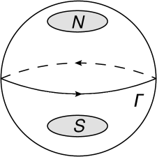
Figure 1: A contour $\Gamma$ divides the Riemann sphere into two hemispheres, with singularities in two regions $N$ and $S$.

We must get the same answer for the integral of eq. (47) if we take the contour to enclose wither $N$ or $S$ (up to a change of sign for differing orientation of the contour). However, we are free to modify the twistor function according to the equivalence relation

$$f(Z^{\alpha})\rightarrow f(Z^{\alpha})+f_{N}(Z^{\alpha})+f_{S}(Z^{\alpha}),$$ (51)

where $f_{N}(Z^{\alpha})$ ($f_{S}(Z^{\alpha})$) contains singularities only in the northern (southern) hemisphere. In carrying out the contour integral for either of $f_{N,S}(Z^{\alpha})$, one may simply choose to enclose the hemisphere that is free of singularities, thus obtaining zero.

The above remarks make clear that the Penrose transform map from twistor space to spacetime is many-to-one. In more mathematical terms, this may be described in terms of sheaf cohomology groups (see e.g. refs. [125, 126] for a review), where the notation ${\rm H}^{1}(\mathbb{PT},{\cal O}(m))$ represents, roughly speaking, the equivalence class of holomorphic functions of homogeneity $m$ in projective twistor space (avoiding the regions $N$ and $S$), modulo the redefinitions of eq. (51). The above Penrose transform then amounts to an isomorphism between massless fields of helicity $n$ in spacetime, and the cohomology group  ${\rm H}^{1}(\mathbb{PT},{\cal O}(-n-2))$.

Above, we have given the Penrose transform for primed fields. A similar formula may be written for unprimed fields, if one instead uses holomorphic functions defined on projective dual twistor space:

$$\psi_{AB\cdots D}(x)=\frac{1}{2\pi i}\oint_{\Gamma}\lambda_{E}\,d\lambda^{E}\,\lambda_{A}\,\lambda_{B}\ldots\lambda_{D}\left[\rho_{x}f(W_{\alpha})\right].$$ (52)

Analogously to eq. (47), this constitutes an isomorphism between massless fields in spacetime with helicity $-n$, and the cohomology group ${\rm H}^{1}(\mathbb{PT}^{*},{\cal O}(-n-2))$. In early works on twistor theory, it was seen as unsatisfactory that both twistors and dual twistors were needed to define fields of arbitrary helicity. This in turn led to the alternative procedure for negative helicity fields [131]

$$\psi_{AB\ldots C}(x)=\frac{1}{2\pi i}\oint\pi_{E^{\prime}}d\pi^{E^{\prime}}\rho_{x}\left[\frac{\partial}{\partial\omega^{A}}\frac{\partial}{\partial\omega^{B}}\ldots\frac{\partial}{\partial\omega^{C}}f(Z^{\alpha})\right],$$ (53)

in which the spinors $\omega^{A}$ are defined in eq. (38). In this formula, the twistor function must now have homogeneity $(n-2)$ for consistency. In terms of the sheaf cohomology groups mentioned above, one has an isomorphism between helicity $-n$ massless fields in spacetime and elements of the cohomology group ${\rm H}^{1}(\mathbb{PT},{\cal O}(n-2))$. From now on, we will loosely use the term function to imply a given representative of the appropriate cohomology class, returning to a discussion of the latter in section 3.4.

Each of eqs. (47, 52, 53) is defined for Minkowski space only. In gauge theory or gravity, they thus give rise to field configurations that satisfy the linearised Yang-Mills or Einstein equations. This does not bother us for the Weyl double copy, all previous examples of which have been linear, but exact, solutions. However, we must bear this in mind when considering generalisations. Full non-linear generalisations of the Penrose transform exist for the (anti-)self-dual sectors of Yang-Mills theory [132] and gravity [133]. Also, even the linear Penrose transform above is more general than it seems. Conformal invariance is manifest in twistor space, so that we expect that the fields obtained from eqs. (47) and (53) can also be transformed to an arbitrary conformally flat spacetime. In fact, the massless free field equation is known to be conformally invariant [124], so this is indeed the case. There is a subtlety, however, regarding scalar fields. From eq. (47), we expect these to be given by contour integrals of the form

$$\phi(x)=\frac{1}{2\pi i}\oint_{\Gamma}\pi_{E^{\prime}}d\pi^{E^{\prime}}[\rho_{x}f(Z^{\alpha})].$$ (54)

We can longer form an equation like eq. (27), as there is nothing for either of the spinor indices in the covariant derivative $\nabla^{AA^{\prime}}$ to contract with. However, one can instead show that eq. (47) is (in conformally flat spacetimes) a solution of the conformally invariant wave equation

$$\left(\Box+\frac{R}{6}\right)\phi=0,$$ (55)

where $R$ is the Ricci scalar.

The above-mentioned many-to-one property of the Penrose transform of eq. (47) means that it is not possible to write a unique inverse transform that fixes a twistor function $f(Z^{\alpha})$ from a given spacetime field. However, there are some tricks for formulating representative twistor functions for spacetime fields possessing certain properties. A particularly useful one is the observation made in ref. [125], relating the poles of twistor functions to principal spinors in spacetime. First, note that the factorisation property of symmetric spinors means that if a given $n$-index spinor has a $k$-fold principal spinor $\xi_{A^{\prime}}$, it will vanish if contracted with $(n-k+1)$ factors of $\xi_{A^{\prime}}$, but not if only $(n-k)$ factors are contracted. To see this, we may write such a spinor’s decomposition into principal spinors as

$$\phi_{A^{\prime}B^{\prime}\dots F^{\prime}}=\underbrace{\xi_{(A^{\prime}}\xi_{B^{\prime}}\ldots\xi_{C^{\prime}}}_{k\ \rm{factors}}\underbrace{\alpha_{D^{\prime}}\beta_{E^{\prime}}\ldots\gamma_{F^{\prime})}}_{(n-k)\ \rm{factors}},$$ (56)

so that contracting this with $(n-k)$ factors of $\xi^{A^{\prime}}$ gives

$$\xi^{D^{\prime}}\xi^{E^{\prime}}\ldots\xi^{F^{\prime}}\phi_{A^{\prime}B^{\prime}\ldots F^{\prime}}=[\alpha\xi][\beta\xi]\ldots[\gamma\xi]\xi_{(A^{\prime}}\xi_{B^{\prime}}\ldots\xi_{C^{\prime})},\quad[\lambda\mu]\equiv\lambda_{A^{\prime}}\mu^{A^{\prime}}.$$ (57)

The various prefactors on the right-hand side are manifestly non-zero, given that none of the spinors $\{\alpha_{A}^{\prime},\beta_{B^{\prime}}\ldots\gamma_{C^{\prime}}\}$ can be proportional to $\xi_{A^{\prime}}$, if they are distinct principal spinors. Contracting with a further factor of $\xi^{A^{\prime}}$ immediately gives a factor of $[\xi\xi]=0$, thus proving the assertion made above. Now consider the spacetime field defined by eq. (47), in the case where the twistor function $f(Z^{\alpha})$ has a pole of order $m$ (where $m\leq n$), which occurs when $\pi_{A^{\prime}}\propto\eta_{A^{\prime}}$. Contracting eq. (47) with $m$ factors of $\eta^{A^{\prime}}$ gives

$$\underbrace{\eta^{A^{\prime}}\eta^{B^{\prime}}\ldots\eta^{C^{\prime}}}_{m\ {\rm factors}}\underbrace{\phi_{A^{\prime}B^{\prime}\ldots C^{\prime}D^{\prime}\ldots F^{\prime}}}_{n\ {\rm indices}}(x)=\frac{1}{2\pi i}\oint_{\Gamma}\pi_{E^{\prime}}d\pi^{E^{\prime}}[\pi\eta]^{m}\pi_{C^{\prime}}\ldots\pi_{F^{\prime}}[\rho_{x}f(Z^{\alpha})].$$ (58)

The factor $[\pi\eta]^{m}$ in the integrand will kill the $m^{\rm th}$-order pole as $\pi_{A^{\prime}}\rightarrow\eta_{A^{\prime}}$, such that the contour integral is zero. By the above remarks, and given that this will not occur if one contracts with only $(m-1)$ factors of $\eta^{A^{\prime}}$, we thus find that in the Penrose transform of eq. (47), the field $\phi_{A^{\prime}B^{\prime}\ldots F^{\prime}}$ has at least a $(n-m+1)$-fold principal spinor $\eta_{A^{\prime}}$, if the twistor function $f(Z^{\alpha})$ has a single $m^{\rm th}$-order pole as $\pi_{A^{\prime}}\rightarrow\eta_{A^{\prime}}$, enclosed by $\Gamma$. Furthermore, if this pole remains present for varying $x^{AA^{\prime}}$, then the twistor function must have the general form [125]

$$f(Z^{\alpha})=\theta_{m}(Z^{\alpha})\{\chi(Z^{\alpha})\}^{-m},$$ (59)

where $\theta_{m}(Z^{\alpha})$, $\chi(Z^{\alpha})$ are homogeneous and holomorphic, $\theta_{m}(Z^{\alpha})$ is regular at the $m$-fold pole we are discussing, and $\chi(Z^{\alpha})$ has a simple zero.

3 A twistorial derivation of the Weyl double copy

In the previous section, we have reviewed various aspects of spinors and twistors, culminating in the Penrose transform of eq. (47), and its related results of eqs. (52, 53). In this section, we show how these results can be used to derive the Weyl double copy of ref. [45], presented here in eq. (32). We will focus on the conjugate form of eq. (32), involving fields with primed indices. From the remarks of section 2.2, this means that we will be concerned with maps from $\mathbb{PT}$ to spacetime, rather than $\mathbb{PT^{*}}$. Changing notation for later convenience, the general (mixed) Weyl double copy may be written as

$$\phi_{A^{\prime}B^{\prime}C^{\prime}D^{\prime}}=\frac{1}{\phi}\phi^{(1)}_{(A^{\prime}B^{\prime}}\phi^{(2)}_{C^{\prime}D^{\prime})}.$$ (60)

Here $\phi$ satisfies the scalar wave equation, and $\phi^{(1,2)}_{A^{\prime}B^{\prime}}$ are two electromagnetic spinors. Then $\phi_{A^{\prime}B^{\prime}C^{\prime}D^{\prime}}$ satisfies the spin-2 case of the massless free field equation of eq. (27), and thus represents a self-dual Weyl spinor. As discussed in the introduction, the Weyl double copy is related to previous exact classical double copies that have appeared in the literature where overlap exists e.g. the Kerr-Schild double copy of ref. [44]. It has been argued to hold for general type D vacuum spacetimes in ref. [45], and also for type N vacuum spacetimes in ref. [128]. However, a number of questions remain:

1. The form of eq. (60) involves a certain product of spinorial quantities, with symmetrisation over the indices. Is there a deeper explanation of where this form comes from?

2. Similarly, why should there be an exact double copy relating fields in position space? The original BCJ double copy for amplitudes [1, 2] involves products in momentum space, which would be expected to lead to a convolution in position space. Indeed, there are alternative double copy formalisms that have exactly this property [93, 134, 95, 135, 96, 136, 100, 99, 137, 138, 102, 103].

3. Does the double copy apply to Petrov types other than type D or N? As already discussed in section 2.1, the form of eqs. (32, 60) would seem to apply for arbitrary Petrov types, although it is not of course guaranteed that the resulting spinorial quantity on the left-hand side will satisfy the spin-2 massless free field equation.

4. Can the Weyl double copy be extended to curved spacetime backgrounds? Preliminary work for the Kerr-Schild double copy implies that exact results are possible in conformally flat spacetimes [49, 48].

Reference [120] recently presented (in a very brief form) a twistor space procedure for deriving the type D Weyl double copy, and also gave an example of a more general solution (of Petrov type III) that could be obtained from eq. (60). We discuss this, with full details that are missing in ref. [120], in the following sections.

3.1 Twistor space picture

Consider a two holomorphic twistor functions $f_{\rm EM}^{(1,2)}(Z^{\alpha})$ of homogeneity $-4$, and a further holomorphic twistor function $f(Z^{\alpha})$ of homogeneity $-2$. By the Penrose transform described here in section 2.2, these will necessarily respectively correspond to electromagnetic spinors $\phi^{(1,2)}_{A^{\prime}B^{\prime}}$ and a scalar field $\phi$ in spacetime. One may then form a product

$$f_{\rm grav.}(Z^{\alpha})=\frac{f^{(1)}_{\rm EM}(Z^{\alpha})\,f^{(2)}_{\rm EM}(Z^{\alpha})}{f(Z^{\alpha})},$$ (61)

such that the function on the left-hand side necessarily has homogeneity $-6$, and thus potentially corresponds to a spacetime field solving the spin-2 massless free field equation i.e. to a self-dual (linearised) gravity solution . All we have done here is use known properties of the Penrose transform. However, the above remarks imply that there might be some sort of relationship between gauge, gravity and scalar fields in spacetime that corresponds to the product of eq. (61). By choosing suitable functions on the right-hand side of eq. (61), we can generate a particular spacetime relationship. We now show that for a suitable choice of twistor functions, this spacetime relationship is precisely the type D Weyl double copy of eq. (60).

To find the appropriate functions, we may rely on the result of eq. (59), namely that a spacetime field possessing a $(n-m+1)$-fold principal spinor must have a $m$-fold pole in twistor space. A type D Weyl spinor has a pair of 2-fold degenerate principal spinors, such that the twistor function $f(Z^{\alpha})$ must have two triple poles. This in turn implies that the function $\chi(Z^{\alpha})$ in eq. (59) has two simple zeros, and thus corresponds to some quadratic form 

$$\chi(Z^{\alpha})=Q_{\alpha\beta}Z^{\alpha}Z^{\beta},$$ (62)

for some constant $Q_{\alpha\beta}$. Let us also define $\theta_{m}$ in eq. (59) to be the simple combinatorial factor

$$\theta_{m}=\frac{1}{m!},$$ (63)

for reasons that will become clear. Then, putting everything together, we may define a family of twistor functions

$$f_{m}(Z^{\alpha})=\frac{1}{m!}\left[Q_{\alpha\beta}Z^{\alpha}Z^{\beta}\right]^{-m},$$ (64)

and our claim is that this will produce a type D Weyl tensor (for $m=3$), that is related to an electromagnetic field strength ($m=2$) and scalar field ($m=1$). To show that this is indeed true, we may carry out the Penrose transform in each case by choosing homogeneous coordinates

$$\pi_{A^{\prime}}=(1,\xi),\quad\xi\in\mathbb{C}$$ (65)

(n.b. we are allowed to do this, given that the integrand of the Penrose transform has homogeneity zero under rescalings of $\pi_{A^{\prime}}$). The quadratic form in eq. (62) is to be evaluated when the incidence relation of eq. (40) is obeyed, namely for $Z^{\alpha}=(ix^{AA^{\prime}}\pi_{A^{\prime}},\pi_{A^{\prime}})$. Substituting eq. (65) then implies

$$\chi(Z^{\alpha})=N^{-1}(x)(\xi-\xi_{1})(\xi-\xi_{2})$$ (66)

in general, where $\xi_{i}\equiv\xi_{i}(x)$ expresses the location of a pole in terms of the variable $\xi$, and $N^{-1}(x)$ is an overall normalisation factor. The dependence of the incidence relation on $x^{AA^{\prime}}$ gives rise to the spacetime dependence of $\{N,\xi_{i}\}$. The measure of the Penrose transform becomes simply

$$\pi^{E^{\prime}}d\pi_{E^{\prime}}=d\xi,$$ (67)

and we can now consider each value of $m$ in turn. For the scalar case of $m=1$, the Penrose transform reduces to

$$\phi =\frac{1}{2\pi i}\oint_{\Gamma}d\xi\frac{N(x)}{(\xi-\xi_{1})(\xi-\xi_{2})}$$

$$=\frac{N(x)}{2\pi i}\oint_{\Gamma}d\xi\frac{1}{(\xi-\xi_{1})(\xi-\xi_{2})}.$$ (68)

The contour $\Gamma$ is defined on the Riemann sphere of $\xi$, such that it separates the poles at $\xi=\xi_{1}$ and $\xi=\xi_{2}$. We may thus evaluate the contour integral by enclosing only one of these poles, which we take to be $\xi=\xi_{1}$. Cauchy’s theorem then tells us that

$$\oint_{\Gamma}\frac{d\xi}{(\xi-\xi_{1})(\xi-\xi_{2})}=\frac{2\pi i}{\xi_{1}-\xi_{2}},$$ (69)

so that we have

$$\phi(x) =\frac{N(x)}{\xi_{1}-\xi_{2}}.$$ (70)

Next, we have the case $m=2$, which gives the Penrose transform

$$\phi_{A^{\prime}B^{\prime}}=\frac{N^{2}(x)}{2\pi i}\frac{1}{2!}\oint_{\Gamma}d\xi\frac{(1,\xi)_{A^{\prime}}(1,\xi)_{B^{\prime}}}{(\xi-\xi_{1})^{2}(\xi-\xi_{2})^{2}}.$$ (71)

We choose to evaluate the integral for each choice of $\{A^{\prime},B^{\prime}\}$ by again enclosing the pole at $\xi=\xi_{1}$. Recalling that if a function $f(z)$ has an $n^{\rm th}$-order pole at $z=c$, the residue associated with the latter is

$${\rm res}(f,c)=\frac{1}{(n-1)!}\lim_{z\rightarrow c}\frac{d^{n-1}}{dz^{n-1}}\left[(z-c)^{n}f(z)\right],$$ (72)

one may then verify the following:

$$\frac{1}{2\pi i}\oint_{\Gamma}d\xi\frac{\xi^{n}}{(\xi-\xi_{1})^{2}(\xi-\xi_{2})^{2}}=-\frac{1}{(\xi_{1}-\xi_{2})^{3}}\times\begin{cases}2,&n=0,\\ (\xi_{1}+\xi_{2}),&n=1,\\ 2\xi_{1}\xi_{2},&n=2,\end{cases}$$ (73)

which in turn implies

$$\phi_{0^{\prime}0^{\prime}}=-\frac{N^{2}(x)}{(\xi_{1}-\xi_{2})^{3}},\quad\phi_{0^{\prime}1^{\prime}}=\phi_{1^{\prime}0^{\prime}}=-\frac{N^{2}(x)}{(\xi_{1}-\xi_{2})^{3}}\frac{1}{2}(\xi_{1}+\xi_{2}),\quad\phi_{1^{\prime}1^{\prime}}=-\frac{N^{2}(x)}{(\xi_{1}-\xi_{2})^{3}}\xi_{1}\xi_{2}.$$ (74)

Alternatively, one may express $\phi_{A^{\prime}B^{\prime}}$ directly in terms of its principal spinors. Defining

$$\alpha_{A^{\prime}}=(1,\xi_{1}),\quad\beta_{A^{\prime}}=(1,\xi_{2}),$$ (75)

eq. (74) is equivalent to

$$\phi_{A^{\prime}B^{\prime}}=-\frac{N^{2}(x)}{(\xi_{1}-\xi_{2})^{3}}\alpha_{(A^{\prime}}\beta_{B^{\prime})}.$$ (76)

Finally, we can examine the case $m=3$, which produces a Weyl spinor as follows:

$$\phi_{A^{\prime}B^{\prime}C^{\prime}D^{\prime}}=\frac{N^{3}(x)}{2\pi i}\frac{1}{3!}\oint_{\Gamma}d\xi\frac{(1,\xi)_{A^{\prime}}(1,\xi)_{B^{\prime}}(1,\xi)_{C^{\prime}}(1,\xi)_{D^{\prime}}}{(\xi-\xi_{1})^{3}(\xi-\xi_{2})^{3}}.$$ (77)

Again using eq. (72), one finds

$$\frac{1}{2\pi i}\oint_{\Gamma}d\xi\frac{\xi^{n}}{(\xi-\xi_{1})^{3}(\xi-\xi_{2})^{3}}=\frac{1}{(\xi_{1}-\xi_{2})^{5}}\times\begin{cases}6,&n=0,\\ 3(\xi_{1}+\xi_{2}),&n=1,\\ \xi_{1}^{2}+4\xi_{1}\xi_{2}+\xi_{2}^{2},&n=2,\\ 3\xi_{1}\xi_{2}(\xi_{1}+\xi_{2}),&n=3,\\ 6\xi_{1}^{2}\xi_{2}^{2},&n=4.\end{cases}$$ (78)

Substituting this into eq. (77), one finds that the result may be written as

$$\phi_{A^{\prime}B^{\prime}C^{\prime}D^{\prime}} =\frac{N^{3}(x)}{(\xi_{1}-\xi_{2})^{5}}\alpha_{(A^{\prime}}\beta_{B^{\prime}}\alpha_{C^{\prime}}\beta_{D^{\prime})}$$

$$=\left[\frac{N(x)}{(\xi_{1}-\xi_{2})}\right]^{-1}\phi_{(A^{\prime}B^{\prime}}\phi_{C^{\prime}D^{\prime})},$$ (79)

where in the second line we have recognised the spin-1 massless field (i.e. an electromagnetic field strength tensor) of eq. (76), and used the symmetrisation property

$$\Psi_{((A^{\prime}B^{\prime})(C^{\prime}D^{\prime}))}=\Psi_{(A^{\prime}B^{\prime}C^{\prime}D^{\prime})},$$ (80)

which holds for an arbitrary spinor $\Psi_{A^{\prime}B^{\prime}C^{\prime}D^{\prime}}$. We may recognise the prefactor in eq. (79) as the inverse of the scalar field of eq. (70). Thus, our choice of twistor functions has provided a scalar, electromagnetic field strength and (linearised) Weyl tensor satisfying

$$\phi_{A^{\prime}B^{\prime}C^{\prime}D^{\prime}}=\frac{1}{\phi}\phi_{(A^{\prime}B^{\prime}}\phi_{C^{\prime}D^{\prime})}.$$ (81)

This is precisely the (primed version of) the Weyl double copy of eq. (32). Some further comments are in order:

• Our choice of the combinatorial factor in eq. (63) is to reproduce the normalisation of the Weyl double copy as given in ref. [45], and one needs such a factor whenever higher-order poles are present. However, the scalar function $S(x)$ is itself only defined up to a constant factor in that paper, so that this is not strictly necessary. Furthermore, we are working with linearised field equations, so that any constant factor is possible.

• The twistor story explains why there is a classical double copy in position space, given that the Penrose transform links twistor functions with spacetime fields. Furthermore, the somewhat mysterious form of eq. (60) is now also explained.

• In the original formulation of the Weyl double copy, there was no clear prescription for fixing the scalar function $S$. Here, we see that it naturally arises as the scalar field $\phi$ obtained from the $m=1$ case of eq. (64).

• Equation (81) is limited to linearised equations of motion only. However, this is not a problem for the spacetimes considered in ref. [45], all of which linearise the Einstein equations, so that the linearised double copy can be promoted to an exact statement.

• The twistor formalism is in principal conformally invariant (at least in those cases in which the twistor functions do not involve the infinity twistors for a given spacetime, that break conformal invariance). This means that the Weyl double copy should immediately extend to conformally flat spacetimes, thus formalising a preliminary observation made in ref. [49]. One could, for example, take a given set of scalar, electromagnetic and gravity fields that are linked by the Weyl double copy, and conformally transform them directly to a desired spacetime, thus achieving a double copy on a curved background. We leave a full investigation of this interesting possibility to future work.

In order for the above to constitute a full derivation of the Weyl double copy, it must be the case that all possible vacuum type D spacetimes can be obtained using twistor functions of the form of eq. (64). That this is indeed the case has been argued by Haslehurst and Penrose in ref. [139], and general arguments may also be given. Type D vacuum solutions are distinguished by the presence of two distinct shear-free null geodesic congruences. All such congruences (in Minkowski space) can be obtained as the zero sets of twistor functions, by a result known as the Kerr theorem (see also e.g. refs. [125, 126]). In the present case, these twistor functions are precisely those appearing in the denominator of eq. (64).

3.2 Example: Schwarzschild & Taub-NUT

A canonical example is that of the Schwarzschild black hole, which is not (anti-)self-dual by itself. However, it is known [69, 68, 53] that duality transformations map out the parameter space of a general Taub-NUT solution with Schwarzschild mass $M$ and NUT charge $N$. Thus, if we restrict to the self-dual part of the Weyl tensor only, we will obtain self-dual Taub-NUT with a fixed relationship between $M$ and $N$. To obtain this using the above construction, one may take a family of functions as in eq. (64), where a suitable choice for $Q_{\alpha\beta}$ is 

$$Q_{\alpha\beta}=\frac{1}{2}\left(\begin{array}[]{rrrr}0&0&0&-1\\ 0&0&1&0\\ 0&1&0&0\\ -1&0&0&0\end{array}\right),$$ (82)

so that the quadratic form in eq. (62) becomes

$$\chi =Z^{1}Z^{2}-Z^{0}Z^{3}$$

$$=\omega^{1}\pi_{0^{\prime}}-\omega^{0}\pi_{1^{\prime}}.$$ (83)

This must be evaluated subject to the incidence relation of eq. (40), where

$$x^{AA^{\prime}}=\frac{1}{\sqrt{2}}\left(\begin{array}[]{cc}t+z&x+iy\\ x-iy&t-z\end{array}\right).$$ (84)

With $\pi_{A^{\prime}}$ given by eq. (65), we then find

$$\chi=-\frac{i}{\sqrt{2}}\left(\xi^{2}(x+iy)+2z\xi-(x-iy)\right).$$ (85)

This has roots at

$$\xi_{1,2}=\frac{-z\pm r}{(x+iy)}=\frac{x-iy}{z\mp r},\quad r=\sqrt{x^{2}+y^{2}+z^{2}},$$ (86)

and comparing eq. (85) with eq. (66), we find

$$N(x)=\frac{i\sqrt{2}}{(x+iy)}.$$ (87)

From eq. (70), the biadjoint scalar function $\phi$ associated with this solution is given by

$$\phi=\frac{i}{r\sqrt{2}}.$$ (88)

This agrees with the function $S(x)$ presented in ref. [45] , up to an overall normalisation constant. However, their function $S(x)$ is itself only defined up to an overall constant, so this is not a problem.

The field strength and Weyl spinors associated with the electromagnetic and gravity solutions will have the form of eqs. (76, 79), where the two principal spinors in the present case are

$$\alpha_{A^{\prime}}=\left(1,\frac{x-iy}{z+r}\right),\quad\beta_{A^{\prime}}=\left(1,\frac{x-iy}{z-r}\right).$$ (89)

We may relate these to the Kerr-Schild double copy of ref. [44] as follows. In a real spacetime, we construct the principal null directions corresponding to the real spinors by combining each of the latter with their complex conjugates and the appropriate Infeld-van-der-Waerden symbols:

$$k^{(1)}_{\mu}=\alpha_{A^{\prime}}\bar{\alpha}_{A}\sigma_{\mu}^{AA^{\prime}},\quad k^{(2)}_{\mu}=\beta_{A^{\prime}}\bar{\beta}_{A}\sigma_{\mu}^{AA^{\prime}}.$$ (90)

Using the spinors of eq. (75), one finds

$$k^{(i)}_{\mu}=\frac{1}{\sqrt{2}}\left(1+|\xi_{i}|^{2},\xi_{i}+\xi_{i}^{*},i(\xi_{i}-\xi_{i}^{*}),1-|\xi_{i}|^{2}\right),$$ (91)

such that the explicit forms of eq. (89) yield

$$k^{(1,2)}_{\mu}\propto\frac{r\sqrt{2}}{r\pm z}\left(1,\pm\frac{x}{r},\pm\frac{y}{r},\pm\frac{z}{r}\right).$$ (92)

The proportional sign here arises from the fact that the spinors of eq. (75) were defined in projective space, and thus can be renormalised by a position-dependent factor. This allows us to remove the prefactor on the right-hand side of eq. (92), and one recovers the two possible choices of Kerr-Schild vector $k_{\mu}$ for the Schwarzschild spacetime [44].

3.3 Examples of general Petrov type

Above, we have seen that it is possible to derive the type D Weyl double copy, by choosing appropriate functions in the twistor space product of eq. (61). However, the spacetime form of the (mixed) double copy, eq. (34), is not intrinsically limited to producing type D solutions only. Thus the question naturally arises as to whether arbitrary Petrov types are possible. This was briefly considered in ref. [120], which presented examples with Petrov types N and III (see also ref. [128] for a discussion of Petrov type N). These examples utilised a particularly well-studied class of holomorphic twistor functions, namely elementary states (see e.g. ref. [125]), which consist of ratios of factors of the form $(A_{\alpha}Z^{\alpha})$, where $A_{\alpha}$ is a constant dual twistor. Elementary states were originally intended as alternatives to plane wave states, for the purposes of examining scattering processes in twistor space. However, they were recently reconsidered from a different point of view, as the twistor functions associated with certain topologically non-trivial electromagnetic fields. Reference [143] pointed out that the field associated with the zeroes of the twistor function $(A_{\alpha}Z^{\alpha})$ is an electromagnetic Hopf knot, any pair of whose electric (or magnetic) field lines are linked. Reference [144] generalised this further, by considering the Penrose transform of the family of twistor functions

$$f_{h}(Z^{\alpha})=(A_{\alpha}Z^{\alpha})^{-1}(B_{\beta}Z^{\beta})^{-2h-1},$$ (93)

where $h$ is the helicity of the resulting field in spacetime. We may write the dual twistors in eq. (93) as 

$$A_{\alpha}=(A_{A},A^{A^{\prime}}),\quad B_{\alpha}=(B_{A},B^{A^{\prime}}).$$ (94)

Furthermore, we follow ref. [144] in defining the calligraphic quantities

$$\rho_{x}[A_{\alpha}Z^{\alpha}]\equiv{\cal A}^{A^{\prime}}\pi_{A^{\prime}},\quad\rho_{x}[B_{\beta}Z^{\beta}]\equiv{\cal B}^{B^{\prime}}\pi_{B^{\prime}},$$ (95)

such that

$${\cal A}^{A^{\prime}}=ix^{AA^{\prime}}A_{A}+A^{A^{\prime}},$$ (96)

and similarly for ${\cal B}^{B^{\prime}}$. Then the corresponding solutions of the massless free field equations were found to be

$$\phi_{A^{\prime}_{1}\ldots A^{\prime}_{2h}}(x)=\left(\frac{2}{\Omega|x-y|^{2}}\right)^{2h+1}{\cal A}_{A^{\prime}_{1}}\ldots{\cal A}_{A^{\prime}_{2h}},$$ (97)

where

$$\Omega=A_{B}B^{B},\quad y^{AA^{\prime}}=i\frac{B^{A}A^{A^{\prime}}-A^{A}B^{A^{\prime}}}{A_{B}B^{B}}.$$ (98)

The spin-1 and spin-2 versions of eq. (97) correspond to a null electromagnetic spinor and type N Weyl spinor respectively. The general field is referred to as a spin-$N$ Hopfion, given that its spacetime topology is related to the well-known Hopf fibration.

A further generalisation was presented in ref. [145], which considered the family of twistor functions

$$f(Z^{\alpha})=\frac{(C_{\gamma}Z^{\gamma})^{h(n_{p}-1)}(D_{\delta}Z^{\delta})^{h(n_{t}-1)}}{(A_{\alpha}Z^{\alpha})(B_{\beta}Z^{\beta})^{h(n_{p}+n_{t})+1}}.$$ (99)

Here $h$ is the helicity as before, and $n_{p},n_{t}\in\mathbb{Z}$. Defining calligraphic spinorial quantities as in eq. (95), the corresponding spacetime fields via the Penrose transform were found to be

$$\phi_{A^{\prime}_{1}\ldots A^{\prime}_{2h}}(x)=\frac{({\cal A}_{C^{\prime}}{\cal C}^{C^{\prime}})^{h(n_{p}-1)}({\cal A}_{D^{\prime}}{\cal D}^{D^{\prime}})^{h(n_{t}-1)}}{({\cal A}_{B^{\prime}}{\cal B}^{B^{\prime}})^{h(n_{p}+n_{t})+1}}{\cal A}_{(A^{\prime}_{1}}\ldots{\cal A}_{A^{\prime}_{2h})}.$$ (100)

These fields again have a non-trivial topology: in the electromagnetic case, electric field lines correspond to torus knots, where $n_{t}$ and $n_{p}$ denote the toroidal and poloidal winding numbers. A similar geometry (involving gravitoelectric field lines, defined from the parity-even part of the Weyl tensor) can be ascertained in the spin-2 case. Again, the electromagnetic field strength is null, and the Weyl spinor is type N. Reference [146] sought to generalise this, by constructing gravitational solutions with different Petrov types. In particular, the following Penrose transform was noted :

$$\frac{1}{(A_{\alpha}Z^{\alpha})^{1+a}(B_{\alpha}Z^{\alpha})^{1+b}} \rightarrow\frac{{\cal N}_{ab}}{[{\cal A}{\cal B}]^{a+b+1}}{\cal A}_{(A^{\prime}_{1}}\ldots{\cal A}_{A^{\prime}_{b}}{\cal B}_{A^{\prime}_{b+1}}\ldots{\cal B}_{A^{\prime}_{2h})}$$

$$={\cal N}_{ab}\left(\frac{2}{\Omega|x-y|^{2}}\right)^{a+b+1}{\cal A}_{(A^{\prime}_{1}}\ldots{\cal A}_{A^{\prime}_{b}}{\cal B}_{A^{\prime}_{b+1}}\ldots{\cal B}_{A^{\prime}_{2h})},$$ (101)

where

$${\cal N}_{ab}=(-1)^{a}\left(\begin{array}[]{c}a+b\\ a\end{array}\right).$$ (102)

The Weyl double copy properties of torus knots were considered using methods similar to refs. [147, 50] in ref. [130], although the form of the biadjoint field was not explicitly discussed there. However, the above results fit very nicely into the twistor space picture for obtaining the Weyl double copy. Starting with eqs. (93, 97), one may take the cases with $h=0$, $h=1$ and $h=2$ as the scalar, electromagnetic and gravity functions in the twistor space product of eq. (61), such that the corresponding spacetime fields are

$$\phi=\frac{2}{\Omega|x-y|^{2}},\quad\phi_{A^{\prime}B^{\prime}}=\left(\frac{2}{\Omega|x-y|^{2}}\right)^{3}{\cal A}_{(A^{\prime}}{\cal A}_{B^{\prime})},\quad\phi_{A^{\prime}B^{\prime}C^{\prime}D^{\prime}}=\left(\frac{2}{\Omega|x-y|^{2}}\right)^{5}{\cal A}_{(A^{\prime}}{\cal A}_{B^{\prime}}{\cal A}_{C^{\prime}}{\cal A}_{D^{\prime})},$$ (103)

from which it is straightforward to verify eq. (34). A similar analysis can be carried out for eqs. (99) and (100).

Next, consider eq. (101). If $a=b=0$, one obtains the scalar field of eq. (103). One may construct twistor functions of homogeneity $-4$ by choosing $(a,b)=(1,1)$ or $(0,2)$, leading to the two respective electromagnetic spinors

$$\phi^{(1,1)}_{A^{\prime}B^{\prime}}=-2\left(\frac{2}{\Omega|x-y|^{2}}\right)^{3}{\cal A}_{(A^{\prime}}{\cal B}_{B^{\prime})},\quad\phi^{(0,2)}_{A^{\prime}B^{\prime}}=\left(\frac{2}{\Omega|x-y|^{2}}\right)^{3}{\cal A}_{(A^{\prime}}{\cal A}_{B^{\prime})}.$$ (104)

Using these in the mixed Weyl double copy of eq. (34), one can generate a number of different Weyl spinors:

$$\phi^{(1,1)\times(1,1)}_{A^{\prime}B^{\prime}C^{\prime}D^{\prime}} =4\left(\frac{2}{\Omega|x-y|^{2}}\right)^{5}{\cal A}_{(A^{\prime}}{\cal A}_{B^{\prime}}{\cal B}_{C^{\prime}}{\cal B}_{D^{\prime})},$$

$$\phi^{(1,1)\times(0,2)}_{A^{\prime}B^{\prime}C^{\prime}D^{\prime}} =-2\left(\frac{2}{\Omega|x-y|^{2}}\right)^{5}{\cal A}_{(A^{\prime}}{\cal A}_{B^{\prime}}{\cal A}_{C^{\prime}}{\cal B}_{D^{\prime})},$$ (105)

$$\phi^{(0,2)\times(0,2)}_{A^{\prime}B^{\prime}C^{\prime}D^{\prime}} =\left(\frac{2}{\Omega|x-y|^{2}}\right)^{5}{\cal A}_{(A^{\prime}}{\cal A}_{B^{\prime}}{\cal A}_{C^{\prime}}{\cal A}_{D^{\prime})},$$ (106)

which is entirely consistent with the rule for combining the corresponding functions in twistor space. The first and third of these examples are Petrov type D and N respectively. However, the second (as already noted in ref. [146]) is Petrov type III, thus going beyond the original formulation of the Weyl double copy in ref. [45].

We may go further than the above (and the results of ref. [120]) by seeking Weyl double copy examples with Petrov types I and II, where again we may rely on elementary states. However, we will see that this leads to a generalisation of the Weyl double copy formula of eq. (60). Let us illustrate this with the simpler case of type II solutions. Consider the twistor function

$$f_{\rm grav.}^{\rm(II)}=\frac{C_{\gamma}Z^{\gamma}}{(A_{\alpha}Z^{\alpha})^{3}(B_{\beta}Z^{\beta})^{4}}\equiv\frac{\mathcal{C}^{E^{\prime}}\pi_{E^{\prime}}}{(\mathcal{A}^{G^{\prime}}\pi_{G^{\prime}})^{3}(\mathcal{B}^{H^{\prime}}\pi_{H^{\prime}})^{4}},$$ (107)

where $A_{\alpha}$, $B_{\alpha}$ and $C_{\alpha}$ are constant dual twistors, and we have defined calligraphic spinors as in eq. (95). This has homogeneity $-6$ and thus represents a gravity solution in spacetime, where the appropriate Penrose transform can be written as

$$\Psi^{\rm(II)}_{A^{\prime}B^{\prime}C^{\prime}D^{\prime}}=\mathcal{C}^{E^{\prime}}\phi_{A^{\prime}B^{\prime}C^{\prime}D^{\prime}E^{\prime}}^{(2,3)},$$ (108)

where

$$\phi_{A^{\prime}B^{\prime}C^{\prime}D^{\prime}E^{\prime}}^{(2,3)} =\frac{1}{2\pi i}\oint_{\Gamma}\frac{\pi_{A^{\prime}}\pi_{B^{\prime}}\pi_{C^{\prime}}\pi_{D^{\prime}}\pi_{E^{\prime}}}{(\mathcal{A}^{G^{\prime}}\pi_{G^{\prime}})^{3}(\mathcal{B}^{H^{\prime}}\pi_{H^{\prime}})^{4}}\pi_{I^{\prime}}d\pi^{I^{\prime}},$$

$$=\frac{10}{[\mathcal{AB}]^{6}}\mathcal{A}_{(A^{\prime}}\mathcal{A}_{B^{\prime}}\mathcal{A}_{C^{\prime}}\mathcal{B}_{D^{\prime}}\mathcal{B}_{E^{\prime})},$$ (109)

and we have used eq. (101) in the second line. To see why eq. (108) yields a type II Weyl spinor, note that one may rewrite the spinorial quantity on the right-hand side of eq. (109) as

$$\mathcal{A}_{(A^{\prime}}\mathcal{A}_{B^{\prime}}\mathcal{A}_{C^{\prime}}\mathcal{B}_{D^{\prime}}\mathcal{B}_{E^{\prime})}=\frac{1}{5}\left[3\mathcal{A}_{E^{\prime}}\mathcal{B}_{(A^{\prime}}+2\mathcal{B}_{E^{\prime}}\mathcal{A}_{(A^{\prime}}\right]\mathcal{A}_{B^{\prime}}\mathcal{A}_{C^{\prime}}\mathcal{B}_{D^{\prime})},$$ (110)

such that the Weyl spinor of eq. (108) may be rewritten as

$$\Psi_{A^{\prime}B^{\prime}C^{\prime}D^{\prime}}^{\rm(II)}=\frac{2}{[\mathcal{AB}]^{5}}\mathcal{A}_{(A^{\prime}}\mathcal{A}_{B^{\prime}}\mathcal{B}_{C^{\prime}}\mathcal{F}_{D^{\prime})},$$ (111)

where

$${\cal F}_{A^{\prime}}=3\frac{[\mathcal{CA}]}{[\mathcal{AB}]}\mathcal{B}_{A^{\prime}}+2\frac{[\mathcal{CB}]}{[\mathcal{AB}]}\mathcal{A}_{A^{\prime}}.$$ (112)

Equation (111) is then manifestly of type II as required, and to show that it may be obtained by a Weyl double copy, we must find twistor functions that can be substituted in eq. (61) so as to reproduce eq. (107). In fact, we need only use the twistor functions related to the electromagnetic Hopfions discussed above. To this end, consider the homogeneity $-4$ functions related to the two electromagnetic spinors (104). These are

$$f^{(0,2)}_{\rm EM} =\frac{1}{(A_{\alpha}Z^{\alpha})(B_{\beta}Z^{\beta})^{3}}=\frac{1}{[\pi{\cal A}][\pi{\cal B}]^{3}},$$

$$f^{(1,1)}_{\rm EM} =\frac{1}{(A_{\alpha}Z^{\alpha})^{2}(B_{\beta}Z^{\beta})^{2}}=\frac{1}{[\pi{\cal A}]^{2}[\pi{\cal B}]^{2}},$$ (113)

where we have used the notations of eqs. (57, 95), as well as the homogeneity $-2$ function

$$f^{(0,0)}=\frac{1}{(A_{\alpha}Z^{\alpha})(B_{\beta}Z^{\beta})}=\frac{1}{[\pi{\cal A}][\pi{\cal B}]}.$$ (114)

Upon applying the Schouten identity

$$[{\cal C}{\cal A}][\pi{\cal B}]+[{\cal B}{\cal C}][\pi{\cal A}]+[{\cal A}{\cal B}][\pi{\cal C}]=0,$$ (115)

one may then rewrite eq. (107) as 

$$f_{\rm grav.}^{\rm(II)}=\frac{1}{f^{(0,0)}}f_{\rm EM}^{\rm(1,1)}\left(-\frac{[{\cal C}{\cal B}]}{[{\cal A}{\cal B}]}f_{\rm EM}^{\rm(0,2)}+\frac{[{\cal C}{\cal A}]}{[{\cal A}{\cal B}]}f_{\rm EM}^{\rm(1,1)}\right).$$ (116)

The spacetime field corresponding to eq. (116) is a Weyl tensor of the form

$$\Psi_{A^{\prime}B^{\prime}C^{\prime}D^{\prime}}^{\rm(II)}=\frac{1}{\phi}\left[3\frac{[{\cal C}{\cal A}]}{[{\cal A}{\cal B}]}\phi^{(0,2)}_{(A^{\prime}B^{\prime}}\phi^{(1,1)}_{C^{\prime}D^{\prime})}-4\frac{[{\cal C}{\cal B}]}{[{\cal A}{\cal B}]}\phi^{(1,1)}_{(A^{\prime}B^{\prime}}\phi^{(1,1)}_{C^{\prime}D^{\prime})}\right],$$ (117)

in agreement with eqs. (111, 112). Here, we have combined the electromagnetic functions to make a gravity function in twistor space, and only then carried out the Penrose transform. This correctly keeps track of combinatorial factors resulting from the multiplicities of the poles in twistor space, and the result of our procedure is that we obtain a generalised double copy formula (eq. (117)), containing a sum of two distinct terms, each with the structure of eq. (60) .

We may carry out a similar analysis for Petrov type I, by considering e.g. the twistor function

$$f_{\rm grav.}^{\rm(I)}=\frac{(\mathcal{C}^{E^{\prime}}\pi_{E^{\prime}})^{2}}{(\mathcal{A}^{G^{\prime}}\pi_{G^{\prime}})^{4}(\mathcal{B}^{H^{\prime}}\pi_{H^{\prime}})^{4}},$$ (118)

whose Penrose transform yields

$$\Psi_{A^{\prime}B^{\prime}C^{\prime}D^{\prime}}^{\rm(I)} = \mathcal{C}^{E^{\prime}}\mathcal{C}^{F^{\prime}}\phi_{A^{\prime}B^{\prime}C^{\prime}D^{\prime}E^{\prime}F^{\prime}}^{(3,3)},$$ (119)

with

$$\phi_{A^{\prime}B^{\prime}C^{\prime}D^{\prime}E^{\prime}F^{\prime}}^{(3,3)} = \frac{1}{2\pi i}\oint\frac{\pi_{A^{\prime}}\pi_{B^{\prime}}\pi_{C^{\prime}}\pi_{D^{\prime}}\pi_{E^{\prime}}\pi_{F^{\prime}}}{(\mathcal{A}^{G^{\prime}}\pi_{G^{\prime}})^{4}(\mathcal{B}^{H^{\prime}}\pi_{H^{\prime}})^{4}}\pi_{I^{\prime}}d\pi^{I^{\prime}}$$ (120)

$$= -\frac{20}{[\mathcal{AB}]^{7}}\mathcal{A}_{(A^{\prime}}\mathcal{A}_{B^{\prime}}\mathcal{A}_{C^{\prime}}\mathcal{B}_{D^{\prime}}\mathcal{B}_{E^{\prime}}\mathcal{B}_{F^{\prime})}.$$

But

$$\mathcal{A}_{(A^{\prime}}\mathcal{A}_{B^{\prime}}\mathcal{A}_{C^{\prime}}\mathcal{B}_{D^{\prime}}\mathcal{B}_{E^{\prime}}\mathcal{B}_{F^{\prime})}=\frac{1}{5}\left[3\mathcal{A}_{(E^{\prime}}\mathcal{B}_{F^{\prime})}\mathcal{A}_{(A^{\prime}}\mathcal{B}_{B^{\prime}}+\mathcal{A}_{E^{\prime}}\mathcal{A}_{F^{\prime}}\mathcal{B}_{(A^{\prime}}\mathcal{B}_{B^{\prime}}+\mathcal{B}_{E^{\prime}}\mathcal{B}_{F^{\prime}}\mathcal{A}_{(A^{\prime}}\mathcal{A}_{B^{\prime}}\right]\mathcal{A}_{C^{\prime}}\mathcal{B}_{D^{\prime})},$$ (121)

such that eq. (119) gives

$$\Psi_{A^{\prime}B^{\prime}C^{\prime}D^{\prime}}^{\rm(I)} =-\frac{4}{[\mathcal{AB}]^{7}}\left[3[\mathcal{CA}][\mathcal{CB}]\mathcal{A}_{(A^{\prime}}\mathcal{B}_{B^{\prime}}+[\mathcal{CA}]^{2}\mathcal{B}_{(A^{\prime}}\mathcal{B}_{B^{\prime}}+[\mathcal{CB}]^{2}\mathcal{A}_{(A^{\prime}}\mathcal{A}_{B^{\prime}}\right]\mathcal{A}_{C^{\prime}}\mathcal{B}_{D^{\prime})}$$

$$=-\frac{1}{[{\cal A}{\cal B}]^{5}}{\cal A}_{(A^{\prime}}{\cal B}_{B^{\prime}}{\cal D}_{C^{\prime}}{\cal E}_{D^{\prime})},$$ (122)

where

$${\cal D}_{C^{\prime}}=(3-\sqrt{5})\frac{[{\cal A}{\cal C}]}{[{\cal A}{\cal B}]}{\cal B}_{C^{\prime}}+\frac{2[{\cal B}{\cal C}]}{[{\cal A}{\cal B}]}{\cal A}_{C^{\prime}},$$

$${\cal E}_{D^{\prime}}=(3+\sqrt{5})\frac{[{\cal A}{\cal C}]}{[{\cal A}{\cal B}]}{\cal B}_{D^{\prime}}+\frac{2[{\cal B}{\cal C}]}{[{\cal A}{\cal B}]}{\cal A}_{C^{\prime}}.$$ (123)

Equation (122) is manifestly of type I as required. As for the type II example of eq. (117), it may be written as a superposition of pure Weyl double copies. By repeated application of eq. (115), we may rewrite the twistor function of eq. (118) as 

$$f_{\rm grav.}^{\rm(I)}=\frac{1}{f^{(0,0)}}\left(\frac{[\mathcal{CB}]}{[\mathcal{AB}]}f^{(0,2)}_{EM}-\frac{[\mathcal{CA}]}{[\mathcal{AB}]}f^{(1,1)}_{EM}\right)\left(-\frac{[\mathcal{CA}]}{[\mathcal{AB}]}f^{(2,0)}_{EM}+\frac{[\mathcal{CB}]}{[\mathcal{AB}]}f^{(1,1)}_{EM}\right),$$ (124)

where we have introduced a third homogeneity $-4$ function

$$f_{\rm EM}^{\rm(2,0)}=\frac{1}{(A_{\alpha}Z^{\alpha})^{3}(B_{\beta}Z^{\beta})}=\frac{1}{[\pi{\cal A}]^{3}[\pi{\cal B}]},$$ (125)

with the respective electromagnetic spinor

$$\phi^{(2,0)}_{A^{\prime}B^{\prime}}=-\left(\frac{2}{\Omega|x-y|^{2}}\right)^{3}{\cal B}_{(A^{\prime}}{\cal B}_{B^{\prime})}.$$ (126)

Expanding and transforming each term separately to position space, one finds

$$\Psi^{\rm(I)}_{A^{\prime}B^{\prime}C^{\prime}D^{\prime}} =\frac{1}{\phi}\left[\frac{3}{2}\frac{[{\cal C}{\cal A}][{\cal C}{\cal B}]}{[{\cal A}{\cal B}]^{2}}\left(\phi^{\rm(0,2)}_{(A^{\prime}B^{\prime}}\phi^{\rm(2,0)}_{C^{\prime}D^{\prime})}-\phi^{\rm(1,1)}_{(A^{\prime}B^{\prime}}\phi^{\rm(1,1)}_{C^{\prime}D^{\prime})}\right)\right.$$

$$\left.\quad\quad+\frac{[{\cal C}{\cal B}]^{2}}{[{\cal A}{\cal B}]^{2}}\phi^{\rm(0,2)}_{(A^{\prime}B^{\prime}}\phi^{\rm(1,1)}_{C^{\prime}D^{\prime})}-\frac{1}{2}\frac{[{\cal C}{\cal A}]^{2}}{[{\cal A}{\cal B}]^{2}}\phi^{\rm(1,1)}_{(A^{\prime}B^{\prime}}\phi^{\rm(2,0)}_{C^{\prime}D^{\prime})}\right].$$ (127)

As in the previous type II example, this is a sum of pure double copy terms. However, in both cases, there is considerable choice in how one presents the final results. Returning to the simpler type II example of eq. (117), one may define the alternative electromagnetic spinor

$$\Phi_{A^{\prime}B^{\prime}}=3\frac{[{\cal C}{\cal A}]}{[{\cal A}{\cal B}]}\phi^{(0,2)}_{A^{\prime}B^{\prime}}-4\frac{[{\cal C}{\cal B}]}{[{\cal A}{\cal B}]}\phi^{(1,1)}_{A^{\prime}B^{\prime}},$$ (128)

which is guaranteed to solve the massless free field equation given that the two terms on the right-hand side are themselves solutions, and thus may be linearly superposed. Equation (117) then becomes

$$\Psi_{A^{\prime}B^{\prime}C^{\prime}D^{\prime}}^{\rm(II)}=\frac{1}{\phi}\Phi_{(A^{\prime}B^{\prime}}\phi^{\rm(1,1)}_{C^{\prime}D^{\prime})},$$ (129)

which is of pure Weyl double copy form. The reader may be worried that there are apparently different double copy formulae that can be written down that relate different electromagnetic solutions to a given gravity solution. However, this is in fact neither surprising nor profound. The Penrose transform used here is limited to the linearised gauge and gravity theories only, as are our examples of gauge / gravity solutions, such that the ambiguity in associating a given gravity solution with a given pair of electromagnetic solutions is precisely that associated with being able to linearly superpose the latter. Notably, the individual terms in eqs. (117, 127) correspond to Weyl spinors of restricted Petrov type, such that the superpositions involved correspond to the known property that, in the linearised theory, one may superpose solutions to create different Petrov types. We have thus succeeded in providing Weyl double copy examples of more general Petrov type, but in a rather artificial way. One may therefore question the utility of the twistor approach (and indeed the Weyl double copy in general) for these solutions. However, what the twistor framework does is provide an interesting way to classify possible double copy formulae, in that the problem of finding the different single copies of a given Weyl tensor amounts to obtaining the different factorizations of the related twistorial function. It also provides a motivation for why particular solutions may be interesting even at linearised level (e.g. the identification of elementary states with Hopfions and torus knots [143, 144, 146, 145]). It would of course be very interesting to find examples of arbitrary Petrov type where exact – or at the very least non-linear – solutions are related.

3.4 A possible objection

In the previous sections, we have outlined a derivation of the Weyl double copy, that relies on a certain product of holomorphic twistor functions in projective twistor space. However, this should rightly incur the wrath of any sensible twistor theorist: as we discussed in section 2.2, the “functions” we have discussed above are not actually functions, but representatives of cohomology classes. Each spin-$n$ (positive helicity) massless free field in spacetime corresponds to a particular element (cohomology class) from the group ${\rm H}^{1}(\mathbb{PT},-n-2)$, and the interpretation of the product of eq. (61) is then not at all clear .

In more pedestrian terms, the twistor function corresponding to a given spacetime field is not unique, but may be redefined by adding functions whose singularities lie on only one side of the contour $\Gamma$ on the Riemann sphere corresponding to a given spacetime point. Then, the product of eq. (61) that is needed to obtain the Weyl double copy in position space appears incompatible with the ability to perform equivalence relations according to eq. (51), in that the order of these operations does not commute. To illustrate this point, it is sufficient to consider redefining the twistor functions in the numerator of eq. (61), according to

$$f_{\rm EM}^{(i)}(Z^{\alpha})\rightarrow\tilde{f}_{\rm EM}^{(i)}(Z^{\alpha})\equiv f_{\rm EM}^{(i)}(Z^{\alpha})+\chi(Z^{\alpha}),$$ (130)

where $\chi(Z^{\alpha})$ has homogeneity $-4$, and contains poles either in the northern or southern hemisphere when restricted to the Riemann sphere of spacetime point $x$, but not both. By construction, the functions $\tilde{f}^{(i)}(Z^{\alpha})$ give rise to the same electromagnetic spinors $\phi^{(i)}_{A^{\prime}B^{\prime}}(x)$ as the functions $f^{(i)}_{\rm EM}(Z^{\alpha})$. However, forming the product of eq. (61) for the redefined functions leads to the twistor function

$$\frac{\tilde{f}^{(1)}_{\rm EM}(Z^{\alpha})\tilde{f}^{(2)}_{\rm EM}(Z^{\alpha})}{f(Z^{\alpha})}=\frac{f^{(1)}_{\rm EM}(Z^{\alpha})f^{(2)}_{\rm EM}(Z^{\alpha})}{f(Z^{\alpha})}+\sum_{i=1}^{2}\frac{\chi(Z^{\alpha})f_{\rm EM}^{(i)}}{f(Z^{\alpha})}+\frac{\chi^{2}(Z^{\alpha})}{f(Z^{\alpha})}.$$ (131)

Both the second and third terms on the right-hand side have homogeneity $-6$, and thus the right-hand side gives rise to a solution of the massless spin 2 free field equation in spacetime. However, the second term on the right-hand side involves the original functions $f_{\rm EM}^{(i)}(Z^{\alpha})$, and thus will have poles in both the northern and southern hemispheres of the Riemann sphere of $x$. Recognising the first term on the right-hand side as our original gravity function in twistor space, we thus see that eq. (131) does not correspond to an equivalence relation of the form of eq. (51). Consequently, the transformation on the right-hand side will gives rise to a different spacetime gravity solution in general.

If we instead take given representative members of the equivalence class of functions for $(f_{\rm EM}^{(i)},f(Z^{\alpha}))$ and form the product of eq. (61), we are indeed free to make redefinitions according to eq. (51). That is, the transformations

$$\frac{f^{(1)}_{\rm EM}(Z^{\alpha})f^{(2)}_{\rm EM}(Z^{\alpha})}{f(Z^{\alpha})}\rightarrow\frac{f^{(1)}_{\rm EM}(Z^{\alpha})f^{(2)}_{\rm EM}(Z^{\alpha})}{f(Z^{\alpha})}+f_{N}(Z^{\alpha})+f_{S}(Z^{\alpha})$$ (132)

do indeed yield equivalent gravity solutions. However, we are then faced with the puzzle of how to pick out what these representative members are meant to be, given that all possible choices of the classes of function entering eq. (61) are meant to be equivalent!

The above puzzle, whilst interesting, does not appear to pose an obstacle to deriving the Weyl double copy in spacetime. All one has to do to achieve the latter is to pick suitable representatives from each cohomology class, chosen by construction so as to obtain the type D Weyl double copy of eq. (60). Put another way, one only needs to verify the following statement: for particular elements (cohomology classes) from the groups ${\rm H}^{1}(\mathbb{PT},-2)$, ${\rm H}^{1}(\mathbb{PT},-4)$ and ${\rm H}^{1}(\mathbb{PT},-6)$, a representative of each class exists such that the corresponding spacetime fields obey eq. (60). This is a much weaker statement than requiring a complete map between the classes themselves i.e. intepreting the product of eq. (61) as providing a general map:

$${\rm H}^{1}(\mathbb{PT},-2)\times{\rm H}^{1}(\mathbb{PT},-4)\times{\rm H}^{1}(\mathbb{PT},-4)\rightarrow{\rm H}^{1}(\mathbb{PT},-6),$$ (133)

which may or may not be achievable. The validity of the weaker statement above is demonstrated explicitly in section 3.1, but whether or not anything more general can be said is certainly worth investigating, as it is clearly related to central questions regarding the validity and scope of the double copy, including to exact solutions of arbitrary Petrov type.

We note also that from a physics point of view, the situation is highly reminiscent of the well-known BCJ double copy for (quantum) scattering amplitudes [1, 2], in which gravity amplitudes are expressed as a sum of terms, each involving a product of kinematic factors $\{n_{i}\}$ obtained from gauge theory amplitudes. These numerators are gauge-dependent, but such that the total amplitude is gauge-invariant. The double copy structure is not manifest in arbitrary gauges, and one must make generalised gauge transformations (including also field definitions in general) in order to put the numerators into a specific “BCJ-dual” form, so that the double copy can be carried out. This problem already occurs at tree-level, and if a given set of such numerators is subjected to a gauge transformation

$$n_{i}\rightarrow n_{i}+\delta_{i}$$ (134)

for some $\delta_{i}$, the double copy formula will generate unwanted terms in the gravity amplitude, that threaten the gauge-invariance of the latter. It is possible to set up the double copy in a more gauge-invariant manner, but at the expense of having to introduce additional correction terms on the gravity side, to cancel out the unwanted contributions [148]. Although the situation here is not exactly identical (i.e. the equivalence transformations of eq. (51) do not correspond to spacetime gauge transformations), it may well be that some similar procedure in twistor space can be defined, so that full invariance with respect to equivalence transformations is made manifest. Any such procedure presumably faces the additional barrier of having to be interpretable in sheaf cohomological terms, but there is again hope. For example, products of twistor space cohomology classes have been discussed in earlier literature regarding twistor diagrams for scattering amplitudes (see e.g. [131, 149] for reviews). Some of these techniques may be adaptable to the present case of classical solutions, and there may also be existing results from the algebraic geometry literature regarding maps similar to those required here (although we do not know of anything at the time of writing).

Throughout, we have been discussing twistor cohomology classes using the language of sheaf cohomology (or alternatively C̆ech cohomology, which is an appropriate approximation). However, another formulation of the Penrose transform exists, in which the twistor functions become differential forms, and are to be interpreted as Dolbeault cohomology classes (see e.g. [150] for a review). That this is equivalent to the above approach follows from known isomorphisms between C̆ech and Dolbeault cohomology groups. It would certainly be interesting to try to reformulate our derivation of the Weyl double copy in the Dolbeault approach, as this is clearly related to whether the double copy has a genuinely twistorial interpretation.

3.5 The Weyl double copy for anti-self-dual fields

In the previous sections, as in ref. [120], we have addressed the Weyl double copy for self-dual fields i.e. those with primed spinor indices. In this section, we extend this discussion to anti-self-dual fields. As reviewed in section 2.2, there are two Penrose transforms one may consider for anti-self-dual fields. The first (eq. (52)) simply consists of replacing twistors with dual twistors, and it is straightforward to see that the derivation of the type D Weyl double copy in terms of anti-self-dual fields proceeds similarly to the case of self-dual fields discussed above. That is, one may consider the family of functions

$$\tilde{f}_{m}=\frac{1}{m!}\left[Q^{\alpha\beta}W_{\alpha}W_{\beta}\right]^{-m},$$ (135)

with $Q^{\alpha\beta}$ a constant matrix. In the Penrose transform, this is to be evaluated subject to the incidence relation of eq. (45), and one may choose homogeneous coordinates

$$\lambda_{A}=(1,\eta)$$ (136)

such that the quadratic form appearing on the right-hand side of eq. (135) may be written as

$$\tilde{\chi}\equiv\rho_{x}\left[Q^{\alpha\beta}W_{\alpha}W_{\beta}\right]=\tilde{{\cal N}}^{-1}(x)(\eta-\eta_{1}(x))(\eta-\eta_{2}(x)),$$ (137)

for some spacetime-dependent functions $\tilde{N}$ and $\eta_{i}$. Carrying out the Penrose transforms for $m\in\{1,2,3\}$ yields spacetime fields

$$S=\frac{\tilde{N}(x)}{\eta_{1}-\eta_{2}},\quad\phi_{AB}=-\frac{\tilde{N}^{2}(x)}{(\eta_{1}-\eta_{2})^{3}}\alpha_{(A}\beta_{B)},\quad\Psi_{ABCD}=\frac{\tilde{N}^{3}(x)}{(\eta_{1}-\eta_{2})^{5}}\alpha_{(A}\beta_{B}\alpha_{C}\beta_{D)},$$ (138)

obeying the Weyl double copy formula of eq. (32).

One may also consider using the (non-dual) twistor space Penrose transform of eq. (53), but the complication then arises of how to form a product in twistor space (i.e. before or after the derivatives are applied). In section 3.1, each quantity entering the twistor space product must be interpretable by itself as corresponding to a spacetime field, after restriction to a given spacetime point. In eq. (53), the restriction to a given spacetime point happens after the function $f(Z^{\alpha})$ has already been differentiated, which suggests that we define a twistor-space product in terms of differentiated quantities:

$$f_{AB\ldots C}=\frac{\partial}{\partial\omega^{A}}\frac{\partial}{\partial\omega^{B}}\ldots\frac{\partial}{\partial\omega^{C}}f(Z^{\alpha}).$$ (139)

A twistorial double copy for anti-self-dual fields can then be written as

$$f^{\rm grav.}_{ABCD}=\frac{f^{\rm EM}_{(AB}f^{\rm EM}_{CD)}}{f}.$$ (140)

We can at least show that such a relationship holds in particular cases. For example, a suitable function to be entered into eq. (53) for the (anti-self-dual) Coulomb solution is [140]

$$f^{\rm EM}=\log\left(\frac{Q}{P}\right),$$ (141)

with

$$P= Z^{2}Z^{3}$$ (142)

$$Q= Z^{1}Z^{2}-Z^{0}Z^{3}\ .$$

From eq. (38), we then find

$$\frac{\partial}{\partial\omega^{A}}P=0\quad\text{and}\quad\frac{\partial}{\partial\omega^{A}}\frac{\partial}{\partial\omega^{B}}Q=0,$$ (143)

so that it is straightforward to compute

$$\tilde{f}^{\rm EM}_{AB}=-\frac{Q_{A}Q_{B}}{Q^{2}},\quad Q_{A}\equiv\frac{\partial}{\partial\omega^{A}}Q.$$ (144)

The anti-self-dual Schwarzschild / Taub-NUT solution can be obtained from the following twistor function for use in eq. (53) [141]:

$$\tilde{f}^{\text{grav}}=\tfrac{1}{2}Q\text{log}\frac{Q}{P}$$ (145)

with $Q$ and $P$ as defined in (142). Then

$$\tilde{f}^{\text{grav}}_{ABCD}=\frac{Q_{A}Q_{B}Q_{C}Q_{D}}{Q^{3}}$$ (146)

Finally, comparing equations (144) and (146), we see that the double copy formula (140) is indeed verified, with

$$f=Q^{-1}$$ (147)

We remark that the expression for the scalar twistor function is the same as that used for the self-dual analysis of section 3.2, as must be the case. Furthermore, different choices of the quadratic form $Q$ (subject to the conditions of eq. (143)) will map out the space of type D vacuum solutions [139].

It is possible to extend the above to general families of solutions. Firstly, recalling the definition of $Z^{\alpha}$ eqn. (39)

$$Z^{\alpha}=(Z^{0},Z^{1},Z^{2},Z^{3})=(\omega^{0},\omega^{1},\pi_{0^{\prime}},\pi_{1^{\prime}})=(\omega^{A},\pi_{A^{\prime}})$$ (148)

we notice that

$$Q=Q_{\alpha\beta}Z^{\alpha}Z^{\beta}=Z^{1}Z^{2}-Z^{0}Z^{3}$$ (149)

was chosen exactly such that

$$Q_{A}=\frac{\partial}{\partial\omega^{A}}Q=(-\pi_{1^{\prime}},\pi_{0^{\prime}})=(\epsilon\pi)_{A},$$ (150)

so that $Q_{A}$ is just $\pi_{A^{\prime}}$ rotated by a Levi-Civita symbol. It is then straightforward to show that we can write

$$\rho_{x}[Q]=(\mathcal{A}^{A^{\prime}}\pi_{A^{\prime}})(\mathcal{B}^{B^{\prime}}\pi_{B^{\prime}})$$ (151)

with $\mathcal{A}^{A^{\prime}}$ and $\mathcal{B}^{B^{\prime}}$ defined as in (96). Then, using (150) and (151) we can write the integrand for the Coulomb solution of (141) as:

$$\rho_{x}\left[\frac{\partial}{\partial\omega^{A}}\frac{\partial}{\partial\omega^{B}}\tilde{f}^{EM}\right]= -(\epsilon\pi)_{A}(\epsilon\pi)_{B}\frac{1}{(\mathcal{A}^{A^{\prime}}\pi_{A^{\prime}})^{2}(\mathcal{B}^{B^{\prime}}\pi_{B^{\prime}})^{2}}$$ (152)

$$= -(\epsilon\pi)_{A}(\epsilon\pi)_{B}f^{(1,1)}_{EM}$$

with $f^{(1,1)}_{EM}$ the function appearing in the self-dual transform (see eq. (113)). Similarly, for the Schwarzschild solution of eq. (145) we have

$$\rho_{x}\left[\frac{\partial}{\partial\omega^{A}}\frac{\partial}{\partial\omega^{B}}\frac{\partial}{\partial\omega^{C}}\frac{\partial}{\partial\omega^{D}}\tilde{f}^{\text{grav}}\right]= 2(\epsilon\pi)_{A}(\epsilon\pi)_{B}(\epsilon\pi)_{C}(\epsilon\pi)_{D}\frac{1}{(\mathcal{A}^{A^{\prime}}\pi_{A^{\prime}})^{3}(\mathcal{B}^{B^{\prime}}\pi_{B^{\prime}})^{3}}$$ (153)

$$= 2(\epsilon\pi)_{A}(\epsilon\pi)_{B}(\epsilon\pi)_{C}(\epsilon\pi)_{D}f^{\rm TypeD}_{\rm grav.}.$$

Above we described the double copy for Type D. In order to progress to more general families, we will first use the results above to find the $\tilde{f}^{\text{EM}}$’s which map to $f^{(0,2)}_{EM}$ and $f^{(2,0)}_{EM}$ defined in (113) and (125). Making the ansatz

$$\tilde{f}^{(0,2)}_{EM}=\frac{Q}{R^{2}}\text{log}\left(\frac{Q}{P}\right)$$ (154)

with $Q$ and $P$ as before and

$$R=R_{\alpha}Z^{\alpha}=R^{A^{\prime}}\pi_{A^{\prime}},$$ (155)

we have

$$\frac{\partial}{\partial\omega^{A}}\frac{\partial}{\partial\omega^{B}}\tilde{f}^{(0,2)}_{EM}=\frac{Q_{A}Q_{B}}{R^{2}Q}.$$ (156)

Then

$$\rho_{x}\left[\frac{\partial}{\partial\omega^{A}}\frac{\partial}{\partial\omega^{B}}\tilde{f}^{(0,2)}_{EM}\right] =(\epsilon\pi)_{A}(\epsilon\pi)_{B}\frac{1}{(\mathcal{A}^{A^{\prime}}\pi_{A^{\prime}})(\mathcal{B}^{B^{\prime}}\pi_{B^{\prime}})(R^{A^{\prime}}\pi_{A^{\prime}})^{2}}$$ (157)

$$\xrightarrow[]{R^{A^{\prime}}=\mathcal{B}^{A^{\prime}}}(\epsilon\pi)_{A}(\epsilon\pi)_{B}f^{(0,2)}_{EM}.$$

Similarly, we have

$$\tilde{f}^{(2,0)}_{EM}=\frac{Q}{S^{2}}\text{log}\left(\frac{Q}{P}\right)$$ (158)

with $Q$ and $P$ as before and

$$S=S_{\alpha}Z^{\alpha}=S^{A^{\prime}}\pi_{A^{\prime}},\qquad S^{A^{\prime}}=\mathcal{A}^{A^{\prime}}.$$ (159)

Finally, the anti-self-dual analogue of the gravity function (118) will be

$$\tilde{f}_{\rm grav.}^{\rm(I)}=\left[\mathcal{G}_{1}Q+\mathcal{G}_{2}\frac{Q^{2}}{R^{2}}+\mathcal{G}_{3}\frac{Q^{2}}{S^{2}}+\mathcal{G}_{4}\frac{Q^{3}}{S^{2}R^{2}}\right]\text{log}\left(\frac{Q}{P}\right)$$ (160)

with $P,Q,R,S$ defined as before. If we choose

$$\mathcal{G}_{1}=-\tfrac{1}{2}\tfrac{[\mathcal{C}\mathcal{A}][\mathcal{C}\mathcal{B}]}{[\mathcal{A}\mathcal{B}]^{2}},\quad\mathcal{G}_{2}=\tfrac{1}{2}\tfrac{[\mathcal{C}\mathcal{B}]^{2}}{[\mathcal{A}\mathcal{B}]^{2}},\quad\mathcal{G}_{3}=\tfrac{1}{2}\tfrac{[\mathcal{C}\mathcal{A}]^{2}}{[\mathcal{A}\mathcal{B}]^{2}},\quad\mathcal{G}_{4}=-\tfrac{1}{6}\tfrac{[\mathcal{C}\mathcal{B}][\mathcal{C}\mathcal{A}]}{[\mathcal{A}\mathcal{B}]^{2}}$$ (161)

then the double copy factorisation proceeds by direct analogy to (124) and the subsequent discussion.

The double copy formula of eq. (140) is perhaps less desirable than the form based on dual twistors, in that it ceases to be a simple product, and thus appears to offer no additional advantages with respect to the spacetime double copy formalism. Note also that the same objections regarding how to interpret the procedure in cohomological terms apply here. The twistor “functions” to be entered into eq. (53) are actually cohomology classes, which in this case are elements of the sheaf cohomology group ${\rm H}^{1}(\mathbb{PT},{\cal O}(n-2))$, for a spin $n$ field. Differentiating $2n$ times maps each cohomology class into an element of ${\rm H}^{1}(\mathbb{PT},{\cal O}(-n-2))$, similar to the case of self-dual fields. Once again, we may take the pragmatic view that in order to generate a particular spacetime double copy, it is sufficient to show that particular representatives of the cohomology classes may be found in twistor space, that achieve the desired spacetime relationship.

4 Conclusion

In this paper, we have examined the Weyl double copy that relates solutions of biadjoint scalar, gauge and gravity theories, using a twistor-space formalism initiated in ref. [120]. The latter argues that each instance of the Weyl double copy in spacetime can be associated with a certain product of functions in twistor space. We have provided full details of how this formalism is sufficient to derive the previously noted form and scope of the Weyl double copy, namely the fact that it applies to arbitrary vacuum type D solutions. We have also gone further than ref. [120] in providing examples of Petrov type I and II solutions in gravity, in addition to types III, D and N. However, such solutions are limited to linearised level, which is ultimately due to the limitations of the Penrose transform itself. We have also shown how similar arguments can be used to derive spacetime double copy formulae for anti-self-dual fields, as well as self-dual ones.

Care must be taken in how to interpret the twistor space double copy, given that it apparently involves multiplying together twistor functions. In the Penrose transform, the “functions” are in fact cohomology classes (i.e. elements of sheaf cohomology groups). Deriving a given instance of the Weyl double copy then amounts to showing the existence of appropriate representations of each cohomology class, such that the functions entering a particular instance of the spacetime Weyl double copy are indeed related by a twistor-space product. This is a far cry from demanding a map between the relevant cohomology groups themselves, and the investigation of whether a more rigorous twistor-space interpretation exists deserves further investigation, as it may shed further light on the ultimate origins and scope of the double copy itself. It may also open up the possibility to look at fully non-linear solutions. Work on these issues is in progress.

References

- [1] Z. Bern, J. J. M. Carrasco, and H. Johansson, “Perturbative Quantum Gravity as a Double Copy of Gauge Theory,” Phys.Rev.Lett. 105 (2010) 061602, 1004.0476.
- [2] Z. Bern, T. Dennen, Y.-t. Huang, and M. Kiermaier, “Gravity as the Square of Gauge Theory,” Phys.Rev. D82 (2010) 065003, 1004.0693.
- [3] H. Kawai, D. Lewellen, and S. Tye, “A Relation Between Tree Amplitudes of Closed and Open Strings,” Nucl.Phys. B269 (1986) 1.
- [4] Z. Bern, L. J. Dixon, D. Dunbar, M. Perelstein, and J. Rozowsky, “On the relationship between Yang-Mills theory and gravity and its implication for ultraviolet divergences,” Nucl.Phys. B530 (1998) 401–456, hep-th/9802162.
- [5] M. B. Green, J. H. Schwarz, and L. Brink, “N=4 Yang-Mills and N=8 Supergravity as Limits of String Theories,” Nucl.Phys. B198 (1982) 474–492.
- [6] Z. Bern, J. Rozowsky, and B. Yan, “Two loop four gluon amplitudes in N=4 superYang-Mills,” Phys.Lett. B401 (1997) 273–282, hep-ph/9702424.
- [7] J. J. Carrasco and H. Johansson, “Five-Point Amplitudes in N=4 Super-Yang-Mills Theory and N=8 Supergravity,” Phys.Rev. D85 (2012) 025006, 1106.4711.
- [8] J. J. M. Carrasco, M. Chiodaroli, M. Günaydin, and R. Roiban, “One-loop four-point amplitudes in pure and matter-coupled N=4 supergravity,” JHEP 1303 (2013) 056, 1212.1146.
- [9] C. R. Mafra and O. Schlotterer, “The Structure of n-Point One-Loop Open Superstring Amplitudes,” JHEP 1408 (2014) 099, 1203.6215.
- [10] R. H. Boels, R. S. Isermann, R. Monteiro, and D. O’Connell, “Colour-Kinematics Duality for One-Loop Rational Amplitudes,” JHEP 1304 (2013) 107, 1301.4165.
- [11] N. E. J. Bjerrum-Bohr, T. Dennen, R. Monteiro, and D. O’Connell, “Integrand Oxidation and One-Loop Colour-Dual Numerators in N=4 Gauge Theory,” JHEP 1307 (2013) 092, 1303.2913.
- [12] Z. Bern, S. Davies, T. Dennen, Y.-t. Huang, and J. Nohle, “Color-Kinematics Duality for Pure Yang-Mills and Gravity at One and Two Loops,” 1303.6605.
- [13] Z. Bern, S. Davies, and T. Dennen, “The Ultraviolet Structure of Half-Maximal Supergravity with Matter Multiplets at Two and Three Loops,” Phys.Rev. D88 (2013) 065007, 1305.4876.
- [14] J. Nohle, “Color-Kinematics Duality in One-Loop Four-Gluon Amplitudes with Matter,” 1309.7416.
- [15] Z. Bern, S. Davies, T. Dennen, A. V. Smirnov, and V. A. Smirnov, “Ultraviolet Properties of N=4 Supergravity at Four Loops,” Phys.Rev.Lett. 111 (2013), no. 23, 231302, 1309.2498.
- [16] S. G. Naculich, H. Nastase, and H. J. Schnitzer, “All-loop infrared-divergent behavior of most-subleading-color gauge-theory amplitudes,” JHEP 1304 (2013) 114, 1301.2234.
- [17] Y.-J. Du, B. Feng, and C.-H. Fu, “Dual-color decompositions at one-loop level in Yang-Mills theory,” 1402.6805.
- [18] C. R. Mafra and O. Schlotterer, “Towards one-loop SYM amplitudes from the pure spinor BRST cohomology,” Fortsch.Phys. 63 (2015), no. 2, 105–131, 1410.0668.
- [19] Z. Bern, S. Davies, and T. Dennen, “Enhanced Ultraviolet Cancellations in N = 5 Supergravity at Four Loop,” 1409.3089.
- [20] C. R. Mafra and O. Schlotterer, “Two-loop five-point amplitudes of super Yang-Mills and supergravity in pure spinor superspace,” 1505.02746.
- [21] S. He, R. Monteiro, and O. Schlotterer, “String-inspired BCJ numerators for one-loop MHV amplitudes,” JHEP 01 (2016) 171, 1507.06288.
- [22] Z. Bern, S. Davies, and J. Nohle, “Double-Copy Constructions and Unitarity Cuts,” 1510.03448.
- [23] G. Mogull and D. O’Connell, “Overcoming Obstacles to Colour-Kinematics Duality at Two Loops,” JHEP 12 (2015) 135, 1511.06652.
- [24] M. Chiodaroli, M. Gunaydin, H. Johansson, and R. Roiban, “Spontaneously Broken Yang-Mills-Einstein Supergravities as Double Copies,” 1511.01740.
- [25] Z. Bern, J. J. M. Carrasco, W.-M. Chen, H. Johansson, R. Roiban, and M. Zeng, “Five-loop four-point integrand of supergravity as a generalized double copy,” Phys. Rev. D96 (2017), no. 12, 126012, 1708.06807.
- [26] H. Johansson and A. Ochirov, “Color-Kinematics Duality for QCD Amplitudes,” JHEP 01 (2016) 170, 1507.00332.
- [27] S. Oxburgh and C. White, “BCJ duality and the double copy in the soft limit,” JHEP 1302 (2013) 127, 1210.1110.
- [28] C. D. White, “Factorization Properties of Soft Graviton Amplitudes,” JHEP 1105 (2011) 060, 1103.2981.
- [29] S. Melville, S. Naculich, H. Schnitzer, and C. White, “Wilson line approach to gravity in the high energy limit,” Phys.Rev. D89 (2014) 025009, 1306.6019.
- [30] A. Luna, S. Melville, S. G. Naculich, and C. D. White, “Next-to-soft corrections to high energy scattering in QCD and gravity,” JHEP 01 (2017) 052, 1611.02172.
- [31] R. Saotome and R. Akhoury, “Relationship Between Gravity and Gauge Scattering in the High Energy Limit,” JHEP 1301 (2013) 123, 1210.8111.
- [32] A. Sabio Vera, E. Serna Campillo, and M. A. Vazquez-Mozo, “Color-Kinematics Duality and the Regge Limit of Inelastic Amplitudes,” JHEP 1304 (2013) 086, 1212.5103.
- [33] H. Johansson, A. Sabio Vera, E. Serna Campillo, and M. A. Vazquez-Mozo, “Color-Kinematics Duality in Multi-Regge Kinematics and Dimensional Reduction,” JHEP 1310 (2013) 215, 1307.3106.
- [34] H. Johansson, A. Sabio Vera, E. Serna Campillo, and M. A. Vazquez-Mozo, “Color-kinematics duality and dimensional reduction for graviton emission in Regge limit,” 1310.1680.
- [35] T. Bargheer, S. He, and T. McLoughlin, “New Relations for Three-Dimensional Supersymmetric Scattering Amplitudes,” Phys.Rev.Lett. 108 (2012) 231601, 1203.0562.
- [36] Y.-t. Huang and H. Johansson, “Equivalent D=3 Supergravity Amplitudes from Double Copies of Three-Algebra and Two-Algebra Gauge Theories,” Phys. Rev. Lett. 110 (2013) 171601, 1210.2255.
- [37] G. Chen and Y.-J. Du, “Amplitude Relations in Non-linear Sigma Model,” JHEP 01 (2014) 061, 1311.1133.
- [38] M. Chiodaroli, Q. Jin, and R. Roiban, “Color/kinematics duality for general abelian orbifolds of N=4 super Yang-Mills theory,” JHEP 01 (2014) 152, 1311.3600.
- [39] H. Johansson and A. Ochirov, “Pure Gravities via Color-Kinematics Duality for Fundamental Matter,” JHEP 11 (2015) 046, 1407.4772.
- [40] H. Johansson and J. Nohle, “Conformal Gravity from Gauge Theory,” 1707.02965.
- [41] M. Chiodaroli, M. Gunaydin, H. Johansson, and R. Roiban, “Gauged Supergravities and Spontaneous Supersymmetry Breaking from the Double Copy Construction,” Phys. Rev. Lett. 120 (2018), no. 17, 171601, 1710.08796.
- [42] G. Chen, H. Johansson, F. Teng, and T. Wang, “On the kinematic algebra for BCJ numerators beyond the MHV sector,” JHEP 11 (2019) 055, 1906.10683.
- [43] C. Cheung and G. N. Remmen, “Entanglement and the Double Copy,” 2002.10470.
- [44] R. Monteiro, D. O’Connell, and C. D. White, “Black holes and the double copy,” JHEP 1412 (2014) 056, 1410.0239.
- [45] A. Luna, R. Monteiro, I. Nicholson, and D. O’Connell, “Type D Spacetimes and the Weyl Double Copy,” Class. Quant. Grav. 36 (2019) 065003, 1810.08183.
- [46] A. Luna, R. Monteiro, D. O’Connell, and C. D. White, “The classical double copy for Taub-NUT spacetime,” Phys. Lett. B750 (2015) 272–277, 1507.01869.
- [47] A. Luna, R. Monteiro, I. Nicholson, D. O’Connell, and C. D. White, “The double copy: Bremsstrahlung and accelerating black holes,” 1603.05737.
- [48] M. Carrillo-González, R. Penco, and M. Trodden, “The classical double copy in maximally symmetric spacetimes,” JHEP 04 (2018) 028, 1711.01296.
- [49] N. Bahjat-Abbas, A. Luna, and C. D. White, “The Kerr-Schild double copy in curved spacetime,” JHEP 12 (2017) 004, 1710.01953.
- [50] D. S. Berman, E. Chacón, A. Luna, and C. D. White, “The self-dual classical double copy, and the Eguchi-Hanson instanton,” 1809.04063.
- [51] I. Bah, R. Dempsey, and P. Weck, “Kerr-Schild Double Copy and Complex Worldlines,” 1910.04197.
- [52] M. Carrillo González, B. Melcher, K. Ratliff, S. Watson, and C. D. White, “The classical double copy in three spacetime dimensions,” JHEP 07 (2019) 167, 1904.11001.
- [53] A. Banerjee, E. Colgáin, J. A. Rosabal, and H. Yavartanoo, “Ehlers as EM duality in the double copy,” 1912.02597.
- [54] A. Ilderton, “Screw-symmetric gravitational waves: a double copy of the vortex,” Phys. Lett. B 782 (2018) 22–27, 1804.07290.
- [55] R. Monteiro, I. Nicholson, and D. O’Connell, “Spinor-helicity and the algebraic classification of higher-dimensional spacetimes,” 1809.03906.
- [56] K. Lee, “Kerr-Schild Double Field Theory and Classical Double Copy,” 1807.08443.
- [57] W. Cho and K. Lee, “Heterotic Kerr-Schild Double Field Theory and Classical Double Copy,” JHEP 07 (2019) 030, 1904.11650.
- [58] K. Kim, K. Lee, R. Monteiro, I. Nicholson, and D. Peinador Veiga, “The Classical Double Copy of a Point Charge,” 1912.02177.
- [59] L. Alfonsi, C. D. White, and S. Wikeley, “Topology and Wilson lines: global aspects of the double copy,” 2004.07181.
- [60] N. Bahjat-Abbas, R. Stark-Muchão, and C. D. White, “Monopoles, shockwaves and the classical double copy,” 2001.09918.
- [61] C. D. White, “Exact solutions for the biadjoint scalar field,” Phys. Lett. B763 (2016) 365–369, 1606.04724.
- [62] P.-J. De Smet and C. D. White, “Extended solutions for the biadjoint scalar field,” Phys. Lett. B775 (2017) 163–167, 1708.01103.
- [63] N. Bahjat-Abbas, R. Stark-Muchão, and C. D. White, “Biadjoint wires,” Phys. Lett. B788 (2019) 274–279, 1810.08118.
- [64] G. Elor, K. Farnsworth, M. L. Graesser, and G. Herczeg, “The Newman-Penrose Map and the Classical Double Copy,” 2006.08630.
- [65] M. K. Gumus and G. Alkac, “More on the classical double copy in three spacetime dimensions,” Phys. Rev. D 102 (2020), no. 2, 024074, 2006.00552.
- [66] C. Keeler, T. Manton, and N. Monga, “From Navier-Stokes to Maxwell via Einstein,” 2005.04242.
- [67] N. Arkani-Hamed, Y.-t. Huang, and D. O’Connell, “Kerr black holes as elementary particles,” JHEP 01 (2020) 046, 1906.10100.
- [68] Y.-T. Huang, U. Kol, and D. O’Connell, “The Double Copy of Electric-Magnetic Duality,” 1911.06318.
- [69] R. Alawadhi, D. S. Berman, B. Spence, and D. Peinador Veiga, “S-duality and the double copy,” JHEP 03 (2020) 059, 1911.06797.
- [70] N. Moynihan, “Kerr-Newman from Minimal Coupling,” JHEP 01 (2020) 014, 1909.05217.
- [71] R. Alawadhi, D. S. Berman, and B. Spence, “Weyl doubling,” JHEP 09 (2020) 127, 2007.03264.
- [72] D. A. Easson, C. Keeler, and T. Manton, “Classical double copy of nonsingular black holes,” Phys. Rev. D 102 (2020), no. 8, 086015, 2007.16186.
- [73] E. Casali and A. Puhm, “A Double Copy for Celestial Amplitudes,” 2007.15027.
- [74] A. Cristofoli, “Gravitational shock waves and scattering amplitudes,” 2006.08283.
- [75] E. Casali and A. Sharma, “Celestial double copy from the worldsheet,” 2011.10052.
- [76] S. Pasterski and A. Puhm, “Shifting Spin on the Celestial Sphere,” 2012.15694.
- [77] T. Adamo and A. Ilderton, “Classical and quantum double copy of back-reaction,” JHEP 09 (2020) 200, 2005.05807.
- [78] G. Alkac, M. K. Gumus, and M. Tek, “The Classical Double Copy in Curved Spacetime,” 2103.06986.
- [79] R. Monteiro, D. O’Connell, D. P. Veiga, and M. Sergola, “Classical Solutions and their Double Copy in Split Signature,” 2012.11190.
- [80] A. Guevara, B. Maybee, A. Ochirov, D. O’connell, and J. Vines, “A worldsheet for Kerr,” JHEP 03 (2021) 201, 2012.11570.
- [81] A. Momeni, J. Rumbutis, and A. J. Tolley, “Kaluza-Klein from Colour-Kinematics Duality for Massive Fields,” 2012.09711.
- [82] A. Luna, R. Monteiro, I. Nicholson, A. Ochirov, D. O’Connell, N. Westerberg, and C. D. White, “Perturbative spacetimes from Yang-Mills theory,” JHEP 04 (2017) 069, 1611.07508.
- [83] W. D. Goldberger and A. K. Ridgway, “Radiation and the classical double copy for color charges,” Phys. Rev. D95 (2017), no. 12, 125010, 1611.03493.
- [84] W. D. Goldberger, S. G. Prabhu, and J. O. Thompson, “Classical gluon and graviton radiation from the bi-adjoint scalar double copy,” Phys. Rev. D96 (2017), no. 6, 065009, 1705.09263.
- [85] W. D. Goldberger and A. K. Ridgway, “Bound states and the classical double copy,” Phys. Rev. D97 (2018), no. 8, 085019, 1711.09493.
- [86] W. D. Goldberger, J. Li, and S. G. Prabhu, “Spinning particles, axion radiation, and the classical double copy,” Phys. Rev. D97 (2018), no. 10, 105018, 1712.09250.
- [87] C.-H. Shen, “Gravitational Radiation from Color-Kinematics Duality,” 1806.07388.
- [88] M. Carrillo-Gonzalez, R. Penco, and M. Trodden, “Radiation of scalar modes and the classical double copy,” 1809.04611.
- [89] J. Plefka, J. Steinhoff, and W. Wormsbecher, “Effective action of dilaton gravity as the classical double copy of Yang-Mills theory,” 1807.09859.
- [90] J. Plefka, C. Shi, J. Steinhoff, and T. Wang, “Breakdown of the classical double copy for the effective action of dilaton-gravity at NNLO,” 1906.05875.
- [91] W. D. Goldberger and J. Li, “Strings, extended objects, and the classical double copy,” 1912.01650.
- [92] A. PV and A. Manu, “Classical double copy from Color Kinematics duality: A proof in the soft limit,” 1907.10021.
- [93] A. Anastasiou, L. Borsten, M. J. Duff, L. J. Hughes, and S. Nagy, “Yang-Mills origin of gravitational symmetries,” Phys. Rev. Lett. 113 (2014), no. 23, 231606, 1408.4434.
- [94] L. Borsten and M. J. Duff, “Gravity as the square of Yang–Mills?,” Phys. Scripta 90 (2015) 108012, 1602.08267.
- [95] A. Anastasiou, L. Borsten, M. J. Duff, M. J. Hughes, A. Marrani, S. Nagy, and M. Zoccali, “Twin supergravities from Yang-Mills theory squared,” Phys. Rev. D96 (2017), no. 2, 026013, 1610.07192.
- [96] G. L. Cardoso, S. Nagy, and S. Nampuri, “A double copy for supergravity: a linearised tale told on-shell,” JHEP 10 (2016) 127, 1609.05022.
- [97] L. Borsten, “On , and theories,” 1708.02573.
- [98] L. Borsten, M. J. Duff, L. J. Hughes, and S. Nagy, “Magic Square from Yang-Mills Squared,” Phys. Rev. Lett. 112 (2014), no. 13, 131601, 1301.4176.
- [99] A. Anastasiou, L. Borsten, M. J. Duff, S. Nagy, and M. Zoccali, “Gravity as Gauge Theory Squared: A Ghost Story,” Phys. Rev. Lett. 121 (2018), no. 21, 211601, 1807.02486.
- [100] G. Lopes Cardoso, G. Inverso, S. Nagy, and S. Nampuri, “Comments on the double copy construction for gravitational theories,” in 17th Hellenic School and Workshops on Elementary Particle Physics and Gravity (CORFU2017) Corfu, Greece, September 2-28, 2017. 2018. 1803.07670.
- [101] A. Luna, S. Nagy, and C. White, “The convolutional double copy: a case study with a point,” JHEP 09 (2020) 062, 2004.11254.
- [102] L. Borsten and S. Nagy, “The pure BRST Einstein-Hilbert Lagrangian from the double-copy to cubic order,” JHEP 07 (2020) 093, 2004.14945.
- [103] Borsten, Leron and Jurco, Branislav and Kim, Hyungrok and Macrelli, Tommaso and Saemann, Christian and Wolf, Martin, “BRST-Lagrangian Double Copy of Yang-Mills Theory,” 2007.13803.
- [104] A. Luna, I. Nicholson, D. O’Connell, and C. D. White, “Inelastic Black Hole Scattering from Charged Scalar Amplitudes,” JHEP 03 (2018) 044, 1711.03901.
- [105] D. A. Kosower, B. Maybee, and D. O’Connell, “Amplitudes, Observables, and Classical Scattering,” JHEP 02 (2019) 137, 1811.10950.
- [106] B. Maybee, D. O’Connell, and J. Vines, “Observables and amplitudes for spinning particles and black holes,” 1906.09260.
- [107] Y. F. Bautista and A. Guevara, “On the Double Copy for Spinning Matter,” 1908.11349.
- [108] Y. F. Bautista and A. Guevara, “From Scattering Amplitudes to Classical Physics: Universality, Double Copy and Soft Theorems,” 1903.12419.
- [109] C. Cheung, I. Z. Rothstein, and M. P. Solon, “From Scattering Amplitudes to Classical Potentials in the Post-Minkowskian Expansion,” 1808.02489.
- [110] Z. Bern, C. Cheung, R. Roiban, C.-H. Shen, M. P. Solon, and M. Zeng, “Black Hole Binary Dynamics from the Double Copy and Effective Theory,” JHEP 10 (2019) 206, 1908.01493.
- [111] Z. Bern, C. Cheung, R. Roiban, C.-H. Shen, M. P. Solon, and M. Zeng, “Scattering Amplitudes and the Conservative Hamiltonian for Binary Systems at Third Post-Minkowskian Order,” Phys. Rev. Lett. 122 (2019), no. 20, 201603, 1901.04424.
- [112] Z. Bern, A. Luna, R. Roiban, C.-H. Shen, and M. Zeng, “Spinning Black Hole Binary Dynamics, Scattering Amplitudes and Effective Field Theory,” 2005.03071.
- [113] G. Kälin and R. A. Porto, “From Boundary Data to Bound States,” JHEP 01 (2020) 072, 1910.03008.
- [114] G. Kälin and R. A. Porto, “Post-Minkowskian Effective Field Theory for Conservative Binary Dynamics,” 2006.01184.
- [115] G. L. Almeida, S. Foffa, and R. Sturani, “Classical Gravitational Self-Energy from Double Copy,” 2008.06195.
- [116] M. Campiglia and S. Nagy, “A double copy for asymptotic symmetries in the self-dual sector,” 2102.01680.
- [117] L. Borsten, I. Jubb, V. Makwana, and S. Nagy, “Gauge x gauge = gravity on homogeneous spaces using tensor convolutions,” to appear.
- [118] L. Borsten, I. Jubb, V. Makwana, and S. Nagy, “Gauge gauge on spheres,” JHEP 06 (2020) 096, 1911.12324.
- [119] L. Borsten, H. Kim, B. Jurco, T. Macrelli, C. Saemann, and M. Wolf, “Double Copy from Homotopy Algebras,” 2102.11390.
- [120] C. D. White, “Twistorial Foundation for the Classical Double Copy,” Phys. Rev. Lett. 126 (2021), no. 6, 061602, 2012.02479.
- [121] R. Penrose, “Twistor algebra,” J. Math. Phys. 8 (1967) 345.
- [122] R. Penrose, “Twistor quantization and curved space-time,” Int. J. Theor. Phys. 1 (1968) 61–99.
- [123] R. Penrose and M. A. H. MacCallum, “Twistor theory: An Approach to the quantization of fields and space-time,” Phys. Rept. 6 (1972) 241–316.
- [124] R. Penrose and W. Rindler, Spinors and Space-Time. Cambridge Monographs on Mathematical Physics. Cambridge Univ. Press, Cambridge, UK, 4, 2011.
- [125] R. Penrose and W. Rindler, SPINORS AND SPACE-TIME. VOL. 2: SPINOR AND TWISTOR METHODS IN SPACE-TIME GEOMETRY. Cambridge Monographs on Mathematical Physics. Cambridge University Press, 4, 1988.
- [126] S. Huggett and K. Tod, AN INTRODUCTION TO TWISTOR THEORY. 9, 1986.
- [127] T. Adamo, “Lectures on twistor theory,” PoS Modave2017 (2018) 003, 1712.02196.
- [128] H. Godazgar, M. Godazgar, R. Monteiro, D. Peinador Veiga, and C. Pope, “The Weyl Double Copy for Gravitational Waves,” 2010.02925.
- [129] J. Stewart, Advanced general relativity. Cambridge Monographs on Mathematical Physics. Cambridge University Press, 4, 1994.
- [130] S. Sabharwal and J. W. Dalhuisen, “Anti-Self-Dual Spacetimes, Gravitational Instantons and Knotted Zeros of the Weyl Tensor,” JHEP 07 (2019) 004, 1904.06030.
- [131] L. Hughston, TWISTORS AND PARTICLES, vol. 97. 1979.
- [132] R. Ward, “On Selfdual gauge fields,” Phys. Lett. A 61 (1977) 81–82.
- [133] R. Penrose, “The Nonlinear Graviton,” Gen. Rel. Grav. 7 (1976) 171–176.
- [134] A. Anastasiou, L. Borsten, M. Hughes, and S. Nagy, “Global symmetries of Yang-Mills squared in various dimensions,” 1502.05359.
- [135] A. Anastasiou, L. Borsten, M. J. Duff, A. Marrani, S. Nagy, and M. Zoccali, “Are all supergravity theories Yang-Mills squared?,” 1707.03234.
- [136] A. Anastasiou, L. Borsten, M. J. Duff, A. Marrani, S. Nagy, and M. Zoccali, “The Mile High Magic Pyramid,” 2017. 1711.08476.
- [137] L. Borsten, “Gravity as the square of gauge theory: a review,”.
- [138] G. Cardoso, S. Nagy, and S. Nampuri, “Multi-centered BPS black holes: a double copy description,” JHEP 04 (2017) 037, 1611.04409.
- [139] L. Haslehurst and R. Penrose, “The most general (2,2) self-dual vacuum,” Twistor Newsletter 34 (1992) 1.
- [140] R. Penrose and G. A. J. Sparling, “The Twistor Quadrille,” Twistor Newsletter 1 (1976) 10.
- [141] G. A. J. Sparling, “The Non-Linear Graviton Representing the Analogue of Schwarzschild or Kerr Black Holes,” Twistor Newsletter 1 (1976) 14.
- [142] L. Hughston et al., eds., ADVANCES IN TWISTOR THEORY. 1, 1979.
- [143] J. Dalhuisen and D. Bouwmeester, “Twistors and electromagnetic knots,” J. Phys. A 45 (2012) 135201.
- [144] J. Swearngin, A. Thompson, A. Wickes, J. W. Dalhuisen, and D. Bouwmeester, “Gravitational Hopfions,” 1302.1431.
- [145] A. Thompson, J. Swearngin, and D. Bouwmeester, “Linked and Knotted Gravitational Radiation,” J. Phys. A 47 (2014) 355205, 1402.3806.
- [146] A. Thompson, A. Wickes, J. Swearngin, and D. Bouwmeester, “Classification of Electromagnetic and Gravitational Hopfions by Algebraic Type,” J. Phys. A 48 (2015), no. 20, 205202, 1411.2073.
- [147] K. P. Tod, “Self dual kerr schild metrics and null Maxwell fields,” Journal of Mathematical Physics 23 (1982), no. 6, 1147–1148, https://doi.org/10.1063/1.525482.
- [148] Z. Bern, J. J. Carrasco, W.-M. Chen, H. Johansson, and R. Roiban, “Gravity Amplitudes as Generalized Double Copies of Gauge-Theory Amplitudes,” Phys. Rev. Lett. 118 (2017), no. 18, 181602, 1701.02519.
- [149] T. N. Bailey and R. J. Baston, eds., Twistors in mathematics and physics, vol. 156. 1990.
- [150] N. M. J. Woodhouse, “REAL METHODS IN TWISTOR THEORY,” Class. Quant. Grav. 2 (1985) 257–291.