DREAM: a fluid-kinetic framework for tokamak disruption runaway electron simulations

Abstract

Avoidance of the harmful effects of runaway electrons (REs) in plasma-terminating disruptions is pivotal in the design of safety systems for magnetic fusion devices. Here, we describe a computationally efficient numerical tool, that allows for self-consistent simulations of plasma cooling and associated RE dynamics during disruptions. It solves flux-surface averaged transport equations for the plasma density, temperature and poloidal flux, using a bounce-averaged kinetic equation to self-consistently provide the electron current, heat, density and RE evolution, as well as the electron distribution function. As an example, we consider disruption scenarios with material injection and compare the electron dynamics resolved with different levels of complexity, from fully kinetic to fluid modes.

PROGRAM SUMMARY
Program Title: Dream
CPC Library link to program files: (to be added by Technical Editor)
Developer’s repository link: https://github.com/chalmersplasmatheory/DREAM
Code Ocean capsule: (to be added by Technical Editor)
Licensing provisions: MIT
Programming language: C++, Python
Nature of problem: Self-consistently simulates the plasma evolution in a tokamak disruption, with specific emphasis on runaway electron dynamics. The runaway electrons can be simulated either as a fluid, fully kinetically, or as a mix of the two. Plasma temperature, current density, electric field, ion density and charge states are all evolved self-consistently, where kinetic non-thermal contributions are captured using an orbit-averaged relativistic electron Fokker-Planck equation, which couples to the plasma evolution. In the typical use case, the electrons are represented by two distinct populations: a cold fluid population and a kinetic superthermal population.
Solution method: The system of equations is solved using a standard multidimensional Newton’s method. Partial differential equations—most prominently the bounce-averaged Fokker–Planck and current diffusion equations—are discretized using a high-resolution finite volume scheme that preserves density and positivity.

1 Introduction

Disruptions of tokamak plasmas involve a partial loss of magnetic confinement and a sudden cooling of the plasma [1]. This thermal quench leads to an increase in the plasma resistivity, causing the plasma current to decay over a period termed the current quench. The toroidal current cannot change significantly on the short thermal quench timescale, and therefore an inductive electric field is produced that can lead to electron runaway. The main runaway generation processes are the Dreicer [2, 3], hot-tail [4, 5, 6] and avalanche [7, 8, 9] mechanisms. In the nuclear phase of operations, these are complemented with electrons generated by the beta decay of tritium and Compton scattering of $\gamma$-rays emitted by the activated wall.

During the current quench, a large part of the plasma current can be converted to a beam of energetic electrons which has the potential to cause severe damage to plasma facing components [10, 11]. As the runaway generation is exponentially sensitive to the plasma current [8], this problem is expected to be unacceptable in future high current tokamaks, such as ITER [1] and SPARC [12]. Development of control methods for avoidance or mitigation of disruptions is therefore of critical importance and urgency in fusion physics.

The most discussed disruption mitigation method is material injection. However, in certain cases the injection of impurities and the associated radiative cooling can lead to the generation of even larger runaway currents [13]. There are a large number of degrees of freedom associated with proposed mitigation methods [14]. However, only a small part of the parameter space is accessible to existing experiments and the extrapolation of the results of existing experiments to next-generation tokamaks is not straightforward [15, 16]. Therefore theoretical modelling and computationally efficient numerical simulations of the disruption and associated runaway electron generation are essential.

Nonlinear magnetohydrodynamic (MHD) simulation tools, such as Jorek [17, 18] and Nimrod [19] have many of the necessary components to simulate mitigated disruptions. However, they so far only allow studies of the dynamics of runaway electrons as test particles [20, 21] or via a fluid model [22, 23, 24], and are computationally expensive. To self-consistently simulate disruption dynamics, an integrated tool that can simulate situations when relativistic electrons comprise a significant part of the electron distribution is required.

Simplified fluid codes such as go [13] and the 1.5-dimensional transport toolkit astra-strahl [25] include kinetically benchmarked models for Dreicer and avalanche runaway electron generation, but have simplified models for hot-tail generation [26]. Fully kinetic tools modelling the momentum-space dynamics of relativistic electrons, such as code [27, 28], norse [29], or the bounce-averaged codes luke [30] and cql3d [4, 31] are suitable for capturing the hot-tail generation, however, to couple these codes to a self-consistent model of the global disruption dynamics leads to prohibitively expensive simulations.

In this paper we describe a new integrated tool for self-consistently simulating the evolution of temperature, poloidal flux, and impurity densities, along with the generation and transport of runaway electrons in tokamaks: Dream (Disruption Runaway Electron Analysis Model). The fully-implicit tool solves a nonlinear set of coupled equations describing the evolution of temperature, density, current density and electric field, as well as the full electron distribution function in arbitrary axisymmetric geometry. It employs a combination of fluid models for background plasma parameters, including the toroidal electric field, electron and ion temperatures, ion densities and charge states, as well as various models for runaway electrons, ranging from fluid to fully kinetic. The most complete drift-kinetic model includes a fully relativistic Fokker-Planck test-particle operator for electron-electron collisions, synchrotron radiation reaction, an avalanche operator, bremsstrahlung and effects of screening in a partially ionized plasma. Neglecting the field-particle part of the collision operator means that the conductivity is underestimated [32], therefore the ohmic current is amended with a conductivity correction to capture the correct Spitzer response to an electric field. A distinguishing feature of Dream is the possibility of choosing reduced kinetic modes, which allow parts of the electron phase space to be modelled kinetically, and the remainder to be described by fluid equations.

The equations that describe the electron kinetics and background plasma evolution in Dream are discussed in Sections 2-3. The numerical implementation is then outlined in Section 4, and benchmarked in Section 5 through a comparison to other numerical tools in various limits. Finally, in Section 6, we use Dream to investigate a disruption simulation in a toroidal plasma, through which we highlight the difference between the hierarchy of electron models implemented.

2 Electron kinetics

Electrons in Dream are primarily modelled with a bounce-averaged drift-kinetic equation of the form

$$\begin{gathered}\frac{\partial f}{\partial t}=\sum_{m,n}\frac{1}{\mathcal{V}^{\prime}}\frac{\partial}{\partial z^{m}}\Bigg{[}\mathcal{V}^{\prime}\Bigg{(}-\left\{A^{m}\right\}f\\ +\left\{D^{mn}\right\}\frac{\partial f}{\partial z^{n}}\Bigg{)}\Bigg{]}+\left\{S\right\},\end{gathered}$$ (1)

where $f(t,\,\boldsymbol{z})$ denotes the electron distribution, $z^{i}$ denotes phase space coordinates and the contravariant components $A^{m}=(\partial z^{m}/\partial\boldsymbol{z})\cdot\boldsymbol{A}$ and (in dyadic notation) $D^{mn}=(\partial z^{m}/\partial\boldsymbol{z})(\partial z^{n}/\partial\boldsymbol{z}):\mathsf{D}$, where $\boldsymbol{A}$ and $\mathsf{D}$ represent the underlying advection vector and diffusion tensor, driving electron phase-space flows. We consider the zero-orbit-width limit, wherein the Larmor radius and cross field drifts are neglected, so that electrons exactly follow magnetic field lines, and choose $\boldsymbol{z}$ as the constants of motion $\boldsymbol{z}=(r,p,\xi_{0})$, where the flux-surface label $r$ is the distance from the magnetic axis when the particle orbit passes the point of minimum magnetic field strength $B_{\mathrm{min}}$; $\xi_{0}=\boldsymbol{B}\cdot\boldsymbol{p}/(Bp)|_{B=B_{\mathrm{min}}}$ is the particle pitch with respect to the magnetic field $\boldsymbol{B}$ at this point and $p$ is the magnitude of the particle momentum. The kinetic equation (1) has been averaged over the remaining three coordinates, using the bounce average denoted with curly brackets

$$\left\{X\right\} =\frac{1}{\mathcal{V}^{\prime}}\int_{0}^{2\pi}\mathrm{d}\zeta\int_{0}^{2\pi}\mathrm{d}\phi\oint\mathrm{d}\theta\sqrt{g}X,$$

$$\mathcal{V}^{\prime} =\int_{0}^{2\pi}\mathrm{d}\zeta\int_{0}^{2\pi}\mathrm{d}\phi\oint\mathrm{d}\theta\sqrt{g},$$ (2)

with toroidal angle $\phi$, gyrophase $\zeta$ and where the angle $\theta$ is an arbitrary poloidal angle which parametrizes the flux surface, assumed to be $2\pi$-periodic. The metric $\sqrt{g}$ of the $(r,\theta,\phi,p,\xi,\zeta)$ coordinates and the spatial Jacobian $\mathcal{J}$ are defined by

$$\sqrt{g} =p^{2}\frac{B}{B_{\mathrm{min}}}\frac{\xi_{0}}{\xi}\mathcal{J},$$

$$\mathcal{J} =\frac{1}{|\nabla\phi\cdot(\nabla\theta\times\nabla r)|},$$ (3)

where $\xi=\mathrm{sgn}(\xi_{0})\sqrt{1-(1-\xi_{0}^{2})B/B_{\mathrm{min}}}$. The poloidal integral along the particle orbit is taken as

$$\oint\mathrm{d}\theta\,X(r,\,\theta,\,\phi,\,p,\,\xi,\,\zeta)$$

$$=\begin{cases}\int_{-\pi}^{\pi}\mathrm{d}\theta\,X(r,\,\theta,\,\phi,\,p,\,\xi,\,\zeta),\hskip 23.90028pt|\xi_{0}|>\xi_{T}\\ \int_{\theta_{b1}}^{\theta_{b2}}\mathrm{d}\theta\,[X(r,\,\theta,\,\phi,\,p,\,\xi,\,\zeta)\\ \hskip 34.1433pt+X(r,\,\theta,\,\phi,\,p,\,-\xi,\,\zeta)],\hskip 8.53581pt0<\xi_{0}\leq\xi_{T}\\ 0,\hskip 110.96574pt-\xi_{T}\leq\xi_{0}\leq 0\end{cases}$$ (4)

where the bounce points $\theta_{b1}$ and $\theta_{b2}$ are the two separate poloidal angles defined by $\xi(\xi_{0},\theta_{b1})=\xi(\xi_{0},\theta_{b2})=0$, and the trapped-passing boundary is denoted $\xi_{T}=\sqrt{1-B_{\mathrm{min}}/B_{\mathrm{max}}}$. In the positive trapped region, $0<\xi_{0}\leq\xi_{T}$, the full contributions from both co-moving and counter-moving trapped particles are accounted for, and therefore all bounce averages are set to zero in $-\xi_{T}\leq\xi_{0}\leq 0$ in order to avoid double counting (in this region the solution satisfies $f(\xi_{0})=f(-\xi_{0})$). We will also utilize the spatial flux surface average

$$\left\langle Y\right\rangle =\frac{1}{V^{\prime}}\int_{0}^{2\pi}\mathrm{d}\phi\int_{-\pi}^{\pi}\mathrm{d}\theta\,\mathcal{J}Y,$$ (5)

$$V^{\prime} =\int_{0}^{2\pi}\mathrm{d}\phi\int_{-\pi}^{\pi}\mathrm{d}\theta\,\mathcal{J}.$$ (6)

The geometry of the magnetic surfaces enters into $\mathcal{J}$ and into the dependence on poloidal angle of $B(\theta)$; in Dream we evolve the equations of motion in a static magnetic geometry where each flux surface is parametrized by its major radius, elongation, Shafranov shift, triangularity and a reference poloidal flux profile, as described in A. The magnetic field is represented by the mixed form

$$\boldsymbol{B}=G\nabla\phi+\frac{1}{2\pi}\nabla\phi\times\nabla\psi,$$ (7)

with $\psi$ the poloidal flux—labeling magnetic surfaces—defined as the magnetic flux through a horizontal disc centred on the tokamak axis of symmetry, as in Ref. [33].

2.1 Kinetic equation

Dream implements the following model for the phase-space advection and diffusion:

$$\boldsymbol{A} =\boldsymbol{A}_{E}+\boldsymbol{A}_{C}+\boldsymbol{A}_{B}+\boldsymbol{A}_{S}+\boldsymbol{A}_{T},$$ (8)

$$\boldsymbol{D} =\mathsf{D}_{C}+\mathsf{D}_{T},$$ (9)

where $\boldsymbol{A}_{E}$ describes acceleration in an electric field, $\boldsymbol{A}_{C}$ collisional friction, $\boldsymbol{A}_{B}$ the bremsstrahlung radiation reaction force, $\boldsymbol{A}_{S}$ the synchrotron radiation reaction force and $\boldsymbol{A}_{T}$ radial transport. Similarly, $\mathsf{D}_{C}$ denotes collisional momentum-space diffusion and $\mathsf{D}_{T}$ radial diffusion. The particle source is modelled as

$$S=C_{\mathrm{ava}}+S_{p},$$ (10)

where $C_{\mathrm{ava}}$ denotes the knock-on collision operator responsible for the runaway avalanche, and $S_{p}$ a particle source to model electron density variations, for example due to ion transport or ionization-recombination.

In the following, we give explicit expressions for these terms in the bounce-averaged electron drift-kinetic equation, as implemented in Dream. For the remainder of the paper, $p=\gamma v/c$ denotes the relativistic momentum normalized to $m_{e}c$, with $\gamma=(1-v^{2}/c^{2})^{-1/2}$ denoting the Lorentz factor and $v$ the speed. Other quantities are given in SI units, except temperatures which have the dimension of energy (the Boltzmann constant is $k_{B}=1$).

2.1.1 Electric field

The acceleration in the parallel electric field is described by the advection term

$$\boldsymbol{A}_{E}=-e\boldsymbol{E},$$ (11)

with the non-vanishing bounce-averaged components

$$\left\{A^{p}_{E}\right\} =-e\left\{E_{\parallel}\xi\right\},$$

$$\left\{A^{\xi_{0}}_{p}\right\} =-e\frac{1-\xi_{0}^{2}}{p\xi_{0}}\left\{E_{\parallel}\xi\right\},$$ (12)

where $E_{\parallel}=\boldsymbol{E}\cdot\boldsymbol{B}/B$, $e$ is the elementary charge, and the average can be written

$$\left\{E_{\parallel}\xi\right\}=2\pi p^{2}\xi_{0}\frac{V^{\prime}}{\mathcal{V}^{\prime}}\frac{\left\langle\boldsymbol{E}\cdot\boldsymbol{B}\right\rangle}{B_{\mathrm{min}}}\times\begin{cases}0,&\text{trapped},\\ 1,&\text{passing}.\end{cases}$$ (13)

2.1.2 Collision operator

Collisions are modelled with a test-particle Fokker-Planck operator consisting of the advection and diffusion terms

$$\mathsf{D}_{C} =m_{e}T_{\mathrm{cold}}\gamma\nu_{s}\hat{p}\hat{p}+m_{e}^{2}c^{2}\frac{\nu_{D}}{2}p^{2}(\mathsf{I}-\hat{p}\hat{p}),$$

$$\boldsymbol{A}_{C} =-\nu_{s}\boldsymbol{p},$$ (14)

with the momentum unit vector $\hat{p}=\boldsymbol{p}/p$. These have the non-vanishing components

$$\left\{D_{C}^{\xi_{0}\xi_{0}}\right\} =(1-\xi_{0}^{2})\frac{\nu_{D}}{2}\left\{\frac{B_{\mathrm{min}}}{B}\frac{\xi^{2}}{\xi_{0}^{2}}\right\},$$

$$\left\{D_{C}^{pp}\right\} =m_{e}T_{\mathrm{cold}}\gamma\nu_{s},$$

$$\left\{A_{C}^{p}\right\} =-p\nu_{s}.$$ (15)

The collision frequencies $\nu_{s}$ and $\nu_{D}$ describe slowing down and pitch-angle scattering and, with the collision operator written in this form, support a Maxwell-Jüttner equilibrium distribution at temperature $T_{\mathrm{cold}}$ independently of their value. These test-particle collision frequencies are given by the sum of the contributions from different sources.

For collisions with free electrons, the collision frequencies are taken from the relativistic Coulomb Fokker-Planck operator [34]

$$\nu_{s}^{\mathrm{ee}} =\nu_{c}\frac{\gamma^{2}\Psi_{1}-\Theta\Psi_{0}+(\Theta\gamma-1)pe^{-(\gamma-1)/\Theta}}{p^{3}e^{1/\Theta}K_{2}(1/\Theta)},$$

$$\nu_{D}^{\mathrm{ee}} =\frac{\nu_{c}}{\gamma p^{5}e^{1/\Theta}K_{2}(1/\Theta)}\biggl{[}(p^{2}\gamma^{2}+\Theta^{2})\Psi_{0}+\Theta(2p^{4}-1)\Psi_{1}$$

$$\hskip 56.9055pt+\gamma\Theta[1+\Theta(2p^{2}-1)]pe^{-(\gamma-1)\Theta}\biggr{]},$$

$$\Psi_{n} =\int_{0}^{p}(1+s^{2})^{(n-1)/2}e^{-(\sqrt{1+s^{2}}-1)/\Theta}\,\mathrm{d}s,$$

$$\Theta =\frac{T_{\mathrm{cold}}}{m_{e}c^{2}},$$

$$\nu_{c} =4\pi\ln\Lambda_{ee}n_{\mathrm{cold}}r_{0}^{2}c,$$ (16)

where $K_{2}$ is the second-order modified Bessel function of the second kind and $r_{0}=e^{2}/(4\pi\varepsilon_{0}m_{e}c^{2})$ the classical electron radius. Here, $n_{\mathrm{cold}}$ and $T_{\mathrm{cold}}$ refer to the density and temperature of the Maxwellian component of the electron distribution, around which the collision operator has been linearized.

Ion collisions, assumed to be against infinitely massive targets, are accounted for using the model presented in Ref. [35], yielding the contributions

$$\nu_{D}^{\mathrm{ei}} =4\pi\frac{\gamma}{p^{3}}cr_{0}^{2}\sum_{i}n_{i}[\ln\Lambda_{ei}Z_{0i}^{2}+g_{i}(p)],$$

$$\nu_{s}^{\mathrm{ei}} =4\pi\frac{\gamma^{2}}{p^{3}}\sum_{i}n_{i}(Z_{i}-Z_{0i})\frac{1}{k}\ln(1+h_{i}^{k}),$$

$$g_{i} =\frac{2}{3}(Z_{i}^{2}-Z_{0i}^{2})\ln(1+(\bar{a}_{i}p)^{3/2})$$

$$\hskip 28.45274pt-\frac{2}{3}(Z_{i}-Z_{0i})^{2}\frac{\bar{a}_{i}p}{1+\bar{a}_{i}p},$$

$$h_{i} =p\sqrt{\gamma-1}\frac{m_{e}c^{2}}{I_{i}}e^{-v^{2}/c^{2}},$$ (17)

where the sum is taken over all ion species (and charge states) in the plasma, $Z_{i}$ denotes their atomic number and $Z_{0i}$ the charge number. The ad-hoc matching parameter $k=5$, and $\bar{a}_{i}$ is an effective-size parameter calculated and tabulated in Ref. [35], or evaluated using the recommended formula $\bar{a}_{i}=(3/2\alpha)(\pi/3)^{1/3}(Z_{i}-Z_{0i})^{2/3}/Z_{i}$, with $\alpha\approx 1/137$ the fine-structure constant, in the absence of tabulated values. The ionic mean-excitation energy $I_{i}$ is calculated using tabulated values from Ref. [36] or extrapolated using their proposed 2-parameter formula for $Z_{i}>18$. The Coulomb logarithms are modelled using

$$\ln\Lambda^{\mathrm{ee}} =\ln\Lambda_{0}+\frac{1}{k}\ln[1+[2(\gamma-1)/p_{Te}^{2}]^{k/2}],$$

$$\ln\Lambda^{\mathrm{ei}} =\ln\Lambda_{0}+\frac{1}{k}\ln[1+(2p/p_{Te})^{k}],$$ (18)

$$\ln\Lambda_{0} =14.9+\ln\left(\frac{T_{\mathrm{cold}}}{1\,\text{keV}}\right)-0.5\ln\left(\frac{n_{\mathrm{free}}}{10^{20}\,\text{m}^{-3}}\right),$$

with the free-electron density $n_{\mathrm{free}}=\sum_{i}Z_{0i}n_{i}$, $p_{Te}=\sqrt{2T_{\mathrm{cold}}/m_{e}c^{2}}$ is the normalized thermal momentum and $k=5$ is a matching parameter analogous to the one appearing in (17).

2.1.3 Radiation reaction force

Radiation losses due to bremsstrahlung are captured using a mean-force model [37]

$$\nu_{s}^{B} =\frac{\gamma}{p}\alpha r_{0}^{2}c\sum_{i}n_{i}Z_{i}^{2}\Biggl{[}\frac{12\gamma^{2}+4}{3\gamma p}\ln(\gamma+p)$$

$$-\frac{8\gamma+6p}{3\gamma p^{2}}\ln^{2}(\gamma+p)-\frac{4}{3}+\frac{2F[2p(\gamma+p)]}{\gamma p}\Biggr{]},$$

$$F(x) =\int_{0}^{x}\frac{\ln(1+y)}{y}\mathrm{d}y,$$ (19)

$$\boldsymbol{A}_{B} =-\nu_{s}^{B}\boldsymbol{p},$$

where effects of straggling [38] and screening are ignored.

Synchrotron emission due to the electron gyromotion around the magnetic field line is accounted for using the advection term

$$\boldsymbol{A}_{S} =-\frac{1}{\gamma\tau_{S}}\left[\boldsymbol{p}_{\perp}+p_{\perp}^{2}\boldsymbol{p}\right],$$

$$\frac{1}{\tau_{S}} =\frac{e^{4}B^{2}}{6\pi\varepsilon_{0}m_{e}^{3}c^{3}},$$ (20)

where $\boldsymbol{p}_{\perp}=\boldsymbol{p}-\boldsymbol{B}\cdot\boldsymbol{p}/B$ denotes the perpendicular momentum. This synchrotron advection term has the components

$$\left\{A_{S}^{p}\right\} =\frac{1}{\tau_{S,\mathrm{min}}}p\gamma(1-\xi_{0}^{2})\left\{\frac{B^{3}}{B_{\mathrm{min}}^{3}}\right\},$$

$$\left\{A_{S}^{\xi_{0}}\right\} =\frac{1}{\tau_{S,\mathrm{min}}}\frac{1}{\gamma}\xi_{0}(1-\xi_{0}^{2})\left\{\frac{B^{2}}{B_{\mathrm{min}}^{2}}\frac{\xi^{2}}{\xi_{0}^{2}}\right\},$$ (21)

where $\tau_{S,\mathrm{min}}=\tau_{S}(B=B_{\mathrm{min}})$.

2.1.4 Avalanche source

Avalanche generation is modelled using the Rosenbluth-Putvinski [8] source term

$$\left\{C_{\mathrm{ava}}\right\} =\left\langle n_{\mathrm{re}}\right\rangle n_{\mathrm{tot}}cr_{0}^{2}\frac{\left\{B\delta(\xi-\xi^{\star})\right\}}{\left\langle B\right\rangle}\frac{1}{p^{2}}\frac{\partial}{\partial p}\frac{1}{1-\gamma},$$

$$\xi^{\star} =\sqrt{\frac{\gamma-1}{\gamma+1}},$$ (22)

where $n_{\mathrm{re}}$ is the density of runaway electrons and $n_{\mathrm{tot}}=\sum_{i}Z_{i}n_{i}$ denotes the total density of electrons (free and bound). The inclusion of bound electrons in this source term provides an approximation for the energy spectrum of electrons created via ionization, which is valid when the energy of the created electron is much greater than the binding energy of the ion [39]. The conservative discretization of this source is detailed in section 4.2.

2.1.5 Radial transport

Radial transport is captured by prescribing the contravariant radial coefficients $A^{r}=(\partial\boldsymbol{x}/\partial r)\cdot\boldsymbol{A}_{T}$ and $D^{rr}=(\partial\boldsymbol{x}/\partial r)(\partial\boldsymbol{x}/\partial r):\mathsf{D}_{T}$. They can either be specified as arbitrary functions of $(t,\,r,\,p,\,\xi_{0})$, or via a Rechester-Rosenbluth model representing diffusion in fully stochastic magnetic field line regions [40]

$$D^{rr}=\pi qR_{\rm m}\left(\frac{\delta B}{B}\right)^{2}|v_{\parallel}|\mathcal{H}(\xi_{0}),$$ (23)

where $(\delta B/B)(r,t)$ represents a normalized radial magnetic field fluctuation amplitude on the flux surface, $R_{\rm m}$ is the major radius of the magnetic axis, $q=q(r)$ is the safety factor calculated from the dynamically evolved plasma current density, and the step function $\mathcal{H}$ equals unity for passing particles and zero for trapped:

$$\mathcal{H}(\xi_{0})=\begin{cases}1,&|\xi_{0}|>\xi_{T}\\ 0,&|\xi_{0}|\leq\xi_{T}\end{cases}$$ (24)

with $\xi_{T}=\sqrt{1-B_{\mathrm{min}}/B_{\mathrm{max}}}$ denoting the trapped-passing boundary. Since the Rechester-Rosenbluth model describes parallel transport along open field lines, trapped particles which bounce back and forth, will not undergo any net radial transport. The bounce average of (23) can concisely be formulated as $\left\{D^{rr}\right\}=\pi qR_{\rm m}c(\delta B/B)^{2}v|\xi_{0}|\left\{\xi/\xi_{0}\right\}$. The heat transport $D_{W}$ associated with this transport model is derived in B.1.

2.1.6 Particle source

In order to describe a time-dependent electron density due to ionization dynamics, an ad-hoc source term is added, of the form

$$\left\{S_{p}\right\}=S_{p}\delta(\boldsymbol{p}),$$ (25)

where electrons are created (or removed) with zero kinetic energy in the ion rest frame. The same source term is used for replacing radially transported fast electrons with cold electrons, required for quasi-neutrality to be maintained. The source amplitude $S_{p}(t,r)$ is treated as an additional unknown quantity which is solved for non-linearly in the Dream equation system, under the constraint of quasineutrality

$$\int\frac{\mathcal{V}^{\prime}}{V^{\prime}}f\,\mathrm{d}p\mathrm{d}\xi_{0}=\sum_{i}Z_{0i}n_{i}.$$ (26)

2.2 Three electron populations

Dream allows the electron distribution to be evolved using the full kinetic equation (1), which is the most accurate but computationally expensive approach. The code also supports the solution of simplified equations for the electron dynamics which often provide adequately accurate results at significantly reduced computational cost. These approximations will be described in this section, and are based on the fact that electron dynamics are qualitatively different on three, typically well separated momentum scales; the corresponding characteristic momenta are

1. The thermal momentum $p_{Te}\sim 0.01$ at which the ohmic current, joule heating and many atomic-physics processes are dominant.

2. The runaway critical momentum $p_{c}\sim\sqrt{E_{c}/E_{\parallel}}\sim 0.1$ at which the runaway generation rate is determined. In this region, electrons that will be thermalized are separated from those runaway electrons that are accelerated towards ultra-relativistic energies.

3. The acceleration region $p\sim\int eE_{\parallel}\,\mathrm{d}t/m_{e}c\sim 100$ where the energy spectrum (and pitch distribution) of the runaway tail is set. The dynamics in this region determine the synchrotron and bremsstrahlung radiation emitted by a runaway beam, as well as the current decay rate during the runaway plateau.

In order to resolve each of these regions efficiently, as well as to allow flexibility in approximating parts of the electron dynamics (such as neglecting to resolve the energy spectrum of the runaway tail if only the generation rate is of interest), electrons in Dream are split into three separate populations: cold, hot and runaway (re) electrons which are, respectively, characterized by the densities $\left\langle n_{\mathrm{cold}}\right\rangle$, $\left\langle n_{\mathrm{hot}}\right\rangle$ and $\left\langle n_{\mathrm{re}}\right\rangle$. These three momentum regions, as well as the two associated electron distribution functions $f_{\mathrm{hot}}$ and $f_{\mathrm{re}}$, are illustrated in figure 1. In the general case, these are distinguished only by labels on different phase-space regions, and the dynamics are purely governed by (1) for all momenta. In the subsections that follow, we describe approximations to the electron kinetics in each of these three regions.

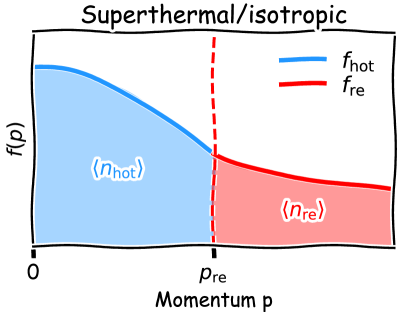
Figure 1: Illustration of the three kinetic regions defined in the fully kinetic mode. In this mode, the distribution function $f_{\rm hot}$ describes both the cold ($p<p_{\mathrm{hot}}$) and hot ($p_{\mathrm{hot}}\leq p<p_{\mathrm{re}}$) electrons, while $f_{\rm re}$ describes the runaway ($p\geq p_{\mathrm{re}}$) electrons on a separate simulation grid.

2.2.1 Cold electrons

The Maxwellian component of the electrons, the cold population, is characterized by the density $\left\langle n_{\mathrm{cold}}\right\rangle$, temperature $T_{\mathrm{cold}}$ and the parallel (ohmic) current density $j_{\Omega}$. The density represents the density of all free electrons that are not labelled hot or runaway:

$$\left\langle n_{\mathrm{cold}}\right\rangle=\left\langle n_{\mathrm{free}}\right\rangle-\left\langle n_{\mathrm{hot}}\right\rangle-\left\langle n_{\mathrm{re}}\right\rangle,$$ (27)

where $\left\langle n_{\mathrm{free}}\right\rangle=\sum_{i}Z_{0i}n_{i}$ is the total number density of free electrons, defined by the ion composition of the plasma, the sum taken over all ion charge states. The temperature is evolved according to a transport equation, to be described further in section 3.

The cold thermal component of the post-disruption plasma is not well-described by the bounce-averaged equation (1) due to its typically high collisionality, and in addition the test-particle collision operator employed in Dream is not adequate for resolving the ohmic current due to the lack of field-particle collisions. Therefore, the ohmic current is modelled according to

$$\frac{j_{\Omega}}{B}=\sigma\frac{\left\langle\boldsymbol{E}\cdot\boldsymbol{B}\right\rangle}{\left\langle B^{2}\right\rangle}+\frac{\delta j_{\mathrm{corr}}}{B},$$ (28)

where $\sigma(n_{i},\,T_{\mathrm{cold}})$ denotes the parallel electric conductivity, and we implement the Sauter-Redl model [41] which accounts for neoclassical effects at arbitrary collisionality. The conductivity correction $\delta j_{\mathrm{corr}}$ is an addition that is used to correct for transient currents when the thermal population is modelled kinetically (see section 2.2.2 below), and is given by

$$\frac{\delta j_{\mathrm{corr}}}{B} =-\frac{2\pi e}{B_{\mathrm{min}}}\int_{0}^{p_{\mathrm{hot}}}\mathrm{d}p\int_{-1}^{1}\mathrm{d}\xi_{0}\,p^{2}\mathcal{H}(\xi_{0})v\xi_{0}f_{\mathrm{hot}}$$

$$-\sigma_{\mathrm{kineq}}\frac{\left\langle\boldsymbol{E}\cdot\boldsymbol{B}\right\rangle}{\left\langle B^{2}\right\rangle},$$ (29)

where the step function $\mathcal{H}$ is defined in (24), $p_{\mathrm{hot}}$ defines a threshold momentum (typically temperature dependent, $p_{\mathrm{hot}}=7p_{Te}$) separating cold from hot electrons, and $\sigma_{\mathrm{kineq}}$ represents the conductivity supported by the kinetic equation (1) in a fully ionized plasma; in such plasmas, $\delta j_{\mathrm{corr}}=0$ in steady state. The $\delta j_{\rm corr}$ term therefore provides a correction to the neoclassical conductivity in a rapidly time-varying plasma and accounts for the effect of partially ionized impurities. By matching the Ohmic conductivity $\sigma_{\rm kineq}$ calculated with the test-particle collision operator for $Z_{\rm eff}\in[0,50]$ to the plasma conductivity calculated in Ref. [42], it was found that the formula

$$\sigma_{\mathrm{kineq}}=\left(1-\frac{1.406}{1.888+Z_{\mathrm{eff}}}\right)\sigma_{0}$$ (30)

provides an accurate approximation, where $\sigma_{0}$ is the Sauter-Redl formula in the collisionless limit.

2.2.2 Hot electrons

The hot electrons, described by a distribution function $f_{\mathrm{hot}}$, are modelled kinetically according to equation (1). They contribute density and parallel current density according to

$$\left\langle n_{\mathrm{hot}}\right\rangle =\int_{p_{\mathrm{hot}}}^{p_{\mathrm{re}}}\mathrm{d}p\int_{-1}^{1}\mathrm{d}\xi_{0}\,\frac{\mathcal{V}^{\prime}}{V^{\prime}}f_{\mathrm{hot}},$$ (31)

$$\frac{j_{\mathrm{hot}}}{B} =-\frac{2\pi e}{B_{\mathrm{min}}}\int_{p_{\mathrm{hot}}}^{p_{\mathrm{re}}}\mathrm{d}p\int_{-1}^{1}\mathrm{d}\xi_{0}\,p^{2}\mathcal{H}(\xi_{0})v\xi_{0}f_{\mathrm{hot}},$$ (32)

where the two threshold momenta $p_{\mathrm{hot}}$ and $p_{\mathrm{re}}$ differentiate hot electrons from cold and runaway electrons, respectively. There are two main modes of treating hot electrons in Dream: the fully kinetic mode where the full distribution function—including the thermal Maxwellian—is resolved kinetically on the grid, and superthermal where only the non-Maxwellian part of the distribution is followed:

Fully kinetic

The full equation (1) is solved, in the form presented in section 2.1. Therefore, thermal electrons are resolved kinetically alongside hot electrons in the distribution function $f_{\rm hot}$ as illustrated in figure 1, since the collision operator is density conserving and drives the solution towards a Maxwell-Jüttner distribution at temperature $T_{\mathrm{cold}}$. In this case, the cold density is given by

$$\left\langle n_{\mathrm{cold}}\right\rangle=\int_{0}^{p_{\mathrm{hot}}}\mathrm{d}p\int_{-1}^{1}\mathrm{d}\xi_{0}\,\frac{\mathcal{V}^{\prime}}{V^{\prime}}f_{\mathrm{hot}},$$ (33)

corresponding to the density of electrons having momentum less than the hot-threshold $p_{\mathrm{hot}}$.

Superthermal

Only the superthermal electrons are resolved by taking the electron-electron collision frequencies as their $T_{\mathrm{cold}}\to 0$ limits

$$\nu_{s}^{\mathrm{ee}} =\frac{\nu_{c}}{pv^{2}/c^{2}},$$

$$\nu_{D}^{\mathrm{ee}} =\frac{\nu_{c}}{p^{2}v/c},$$ (34)

in which case the kinetic equation will no longer support a Maxwellian equilibrium distribution, but instead acquires a particle sink at $p=0$ since the advective particle flux $\lim_{p\to 0}\mathcal{V}^{\prime}p\nu_{s}$ is finite. In this case, the hot-electron threshold is chosen to be $p_{\mathrm{hot}}=0$, meaning that all electrons in $f_{\mathrm{hot}}$ are considered hot, as illustrated in figure 2. By the cold-density equation (27), the electrons that are lost at $p=0$ will be added to $\left\langle n_{\mathrm{cold}}\right\rangle$. In this mode, the conductivity correction $\delta j_{\mathrm{corr}}$ in equation (2.2.1) is dropped since ohmic current is not resolved kinetically. This approach was pioneered in Ref. [6] for thermal quench simulations.

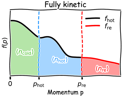
Figure 2: Illustration of how the distribution functions $f_{\rm hot}$ and $f_{\rm re}$ are defined in the superthermal mode. In this mode, the hot electron distribution function $f_{\rm hot}$ covers only the hot region which is extended to $p=0$, while cold electrons are modelled off the grid as a fluid of density $\left\langle n_{\mathrm{cold}}\right\rangle$ and ohmic parallel current density $j_{\Omega}/B$.

Isotropic

A further approximate form of the superthermal mode is supported by Dream, where the kinetic equation is analytically pitch-angle averaged based on an asymptotic expansion in which pitch-angle scattering is assumed to dominate the electron dynamics. The procedure mirrors the approximations employed in the calculation of the avalanche growth rate in ref. [8], but is generalized here to time-dependent situations which covers hot-tail formation. Details on the derivation of this reduced kinetic equation are provided in B.2, and the resulting expression is given by (92).

Table 1: Summary of the approximations used in the four main operating modes of Dream. In the fluid, isotropic and superthermal modes, the cold electrons are represented with a fluid model (here indicated with the density $n_{\rm cold}$ and temperature $T_{\rm cold}$). Notably, the representation of the hot population varies between the models, being represented either as part of the same distribution function $f_{\rm hot}$ as the thermal electrons (fully kinetic), with a distribution function in the superthermal limit (superthermal), with an energy distribution in the superthermal limit (isotropic), or not at all (fluid).

	Cold/thermal electrons	Hot electrons
Fluid	$n_{\rm cold},T_{\rm cold}$	(not modelled)
Isotropic	$n_{\rm cold},T_{\rm cold}$	$\int\mathrm{d}\xi_{0}\,f_{\rm hot}$ ($v\gg v_{\rm th}$)
Superthermal	$n_{\rm cold},T_{\rm cold}$	$f_{\rm hot}$ ($v\gg v_{\rm th}$)
Fully kinetic	$f_{\rm hot}$	$f_{\rm hot}$

2.2.3 Runaway electrons

Runaways are described by the distribution function $f_{\mathrm{re}}$, which satisfies the same kinetic equation as the hot electrons $f_{\mathrm{hot}}$, but is defined on a separate grid spanning the interval $p\in[p_{\mathrm{re}},\,p_{\mathrm{max}}]$, where the runaway threshold is typically chosen as $p_{\mathrm{re}}\sim 1$, and the maximum resolved momentum is $p_{\mathrm{max}}\sim 100$. Note that the boundary $p_{\rm re}$ for the runaway grid is distinct from the usual critical momentum for runaway $p_{\rm c}$ sometimes used to define a runaway electron in other codes. The runaway boundary $p_{\rm re}$ used in Dream is constant in the simulation and must be appropriately chosen by the user so that both the hot and runaway electron distribution functions can be well approximated numerically. As long as the numerical grid is sufficiently resolved, the choice of the boundary $p_{\rm re}$ has no effect on the simulation results.

The reason for separating hot and runaway electrons is that the electron distribution in the hot generation region ($p\sim p_{c}$) is nearly isotropic, whereas in the runaway tail it can be extremely anisotropic. By utilizing a separate grid, resolution and discretization methods can be tailored to more efficiently resolve the runaway tail. Although the runaway electron distribution couples relatively weakly to the plasma evolution since they move with parallel velocities near the speed of light, the runaway distribution is essential when coupling to synthetic radiation diagnostic tools [43, 44] or when considering kinetic instabilities driven by the runaways [45, 46].

Particle conservation is ensured by enforcing a boundary condition on $f_{\mathrm{re}}$ at the lower $p$ boundary

$$F_{\mathrm{re}} =F_{\mathrm{hot}}+\left(\frac{\partial\left\langle n_{\mathrm{re}}\right\rangle}{\partial t}\right)_{\mathrm{fluid}},$$

$$F_{\mathrm{hot/re}} =$$ (35)

$$\int\mathcal{V}^{\prime}\Bigg{(} \left\{A^{p}\right\}f_{\mathrm{hot/re}}+\left\{D^{pp}\right\}\frac{\partial f_{\mathrm{hot/re}}}{\partial p}\Bigg{)}\,\mathrm{d}\xi_{0}\Bigg{|}_{p=p_{\mathrm{re}}}$$

using a method described in section 4.5, where $F_{\mathrm{hot/re}}$ denotes the particle flux through the shared $p=p_{\mathrm{re}}$ boundary on the respective kinetic grids, and $(\partial\left\langle n_{\mathrm{re}}\right\rangle/\partial t)_{\mathrm{fluid}}$ denotes the runaway generation rate due to sources that are not modelled kinetically on the hot grid. An example of such a source is Dreicer generation when using the superthermal mode, in which case the thermal Maxwellian is not resolved so that no electrons are available for Dreicer acceleration. The runaway density, corresponding to the number density of $f_{\mathrm{re}}$, therefore evolves according to

$$\frac{\partial\left\langle n_{\mathrm{re}}\right\rangle}{\partial t} =F_{\mathrm{hot}}+\left(\frac{\partial\left\langle n_{\mathrm{re}}\right\rangle}{\partial t}\right)_{\mathrm{fluid}}$$

$$+\frac{1}{V^{\prime}}\frac{\partial}{\partial r}\left[V^{\prime}\left(A^{r}_{\mathrm{re}}\left\langle n_{\mathrm{re}}\right\rangle+D^{rr}_{\mathrm{re}}\frac{\partial\left\langle n_{\mathrm{re}}\right\rangle}{\partial r}\right)\right].$$ (36)

If the runaway electron distribution function is solved for, the transport term in equation (2.2.3) is replaced with a source term which is the momentum-space integral of the transport term in the kinetic equation (1):

$$\begin{gathered}\left(\frac{\partial\left\langle n_{\mathrm{re}}\right\rangle}{\partial t}\right)_{\rm transport}=\frac{1}{V^{\prime}}\frac{\partial}{\partial r}\Bigg{[}V^{\prime}\\ \times\int\mathrm{d}p\mathrm{d}\xi_{0}\,\mathcal{V}^{\prime}\,\left(A^{r}f_{\mathrm{re}}+D^{rr}\frac{\partial f_{\mathrm{re}}}{\partial r}\right)\Bigg{]}.\end{gathered}$$ (37)

In case the runaway electron distribution function is not explicitly evolved, the transport coefficients can instead be directly prescribed as functions of only radius, or be integrated over momentum space in the manner described in Ref. [47]. The parallel runaway current density is defined as

$$\frac{j_{\mathrm{re}}}{B}=-\frac{2\pi e}{B_{\mathrm{min}}}\int_{p_{\mathrm{re}}}^{p_{\mathrm{max}}}\mathrm{d}p\int_{-1}^{1}\mathrm{d}\xi_{0}\,p^{2}\mathcal{H}(\xi_{0})v\xi_{0}f_{\mathrm{re}}.$$ (38)

The fluid runaway rate $(\partial\left\langle n_{\mathrm{re}}\right\rangle/\partial t)_{\mathrm{fluid}}$ depends on the kinetic model employed, and support is implemented for modelling runaway generation due to Dreicer, hot-tail, Compton, tritium-decay and avalanche [13, 48] depending on which equation terms are enabled. The fluid runaway models are described in C. If the hot grid is disabled altogether, the runaway distribution $f_{\mathrm{re}}$ can still be evolved using fluid models for the generation via the boundary condition (2.2.3). Likewise, if the runaway grid is disabled, runaway generation is still captured via (2.2.3) where transport coefficients $A_{\mathrm{re}}$ and $D_{\mathrm{re}}$ can be imposed. In this case, the runaway current is instead determined by

$$\frac{j_{\mathrm{re}}}{B}=\frac{ec\left\langle n_{\mathrm{re}}\right\rangle}{\left\langle B\right\rangle}.$$ (39)

If neither hot or runaway electrons are resolved kinetically, a fully fluid-like system is obtained, corresponding approximately to the model contained in the Go code [13, 49, 50], generalized here to account for effects of arbitrary axisymmetric toroidal geometry.

3 Background plasma evolution

Dream utilizes a test-particle collision operator for the electron dynamics, which refers to the Maxwellian electron component of the plasma as well as the ion composition. In order to close the equation system, equations governing the evolution of these quantities as well as the electric field must be introduced. In this section we describe the evolution of the background plasma and how it couples to the electrons.

Most equations for the background plasma can be written in the one-dimensional transport equation form

$$\begin{gathered}\frac{\partial X}{\partial t}=\frac{1}{V^{\prime}}\frac{\partial}{\partial r}\left[V^{\prime}\left(-\left\langle A^{r}\right\rangle X+\left\langle D^{rr}\right\rangle\frac{\partial X}{\partial r}\right)\right]\\ +\left\langle S\right\rangle,\end{gathered}$$ (40)

which has a structure very similar to the kinetic equation (1), but only evolves the quantity $X$ in the radial coordinate $r$. In addition, it has the spatial Jacobian $V^{\prime}$ instead of the full phase-space Jacobian $\mathcal{V}^{\prime}$, and uses flux surface averages for its coefficients, defined by (5), instead of bounce averages. The similar structure is utilized when implementing the equations, as the discretized forms of the equations are near identical with only coefficients differing.

3.1 Ions

Ions are modelled by the densities $n_{i}^{(j)}$ of each species $i$ with atomic number $Z_{i}$, and charge state $j$ with charge number $Z_{0j}$, which are assumed to be uniformly distributed on flux surfaces. They are evolved according to

$$\frac{\partial n_{i}^{(j)}}{\partial t} =\left(I_{i}^{(j-1)}\left\langle n_{\mathrm{cold}}\right\rangle+\left\langle\sigma_{\mathrm{ion},i}^{(j-1)}v\right\rangle\right)n_{i}^{(j-1)}$$

$$-\left(I_{i}^{(j)}\left\langle n_{\mathrm{cold}}\right\rangle+\left\langle\sigma_{\mathrm{ion},i}^{(j)}v\right\rangle\right)n_{i}^{(j)}$$

$$+R_{i}^{(j+1)}\left\langle n_{\mathrm{cold}}\right\rangle n_{i}^{(j+1)}-R_{i}^{(j)}\left\langle n_{\mathrm{cold}}\right\rangle n_{i}^{(j)},$$ (41)

where $I$ and $R$ denote ionization and recombination rate coefficients, respectively, which are extracted from the OpenADAS database [51]. The kinetic ionization rates are modelled by

$$\left\langle\sigma_{\mathrm{ion},i}^{(j)}v\right\rangle=\int\mathrm{d}p\int_{-1}^{1}\mathrm{d}\xi_{0}\,\frac{\mathcal{V}^{\prime}}{V^{\prime}}v\sigma_{\mathrm{ion},i}^{(j)}f_{\mathrm{hot/re}},$$ (42)

where the ionization cross-sections $\sigma_{\mathrm{ion},i}^{(j)}$ are taken as in Ref. [52], which extended the validity of the Burgess-Chidichimo model [53] to relativistic energies, with the momentum integration limits taken as in section 2.2. Unlike the cited studies where model parameters were chosen from atomic data, Dream uses parameters which have been fitted to the OpenADAS ionization coefficients in the low-density (coronal) limit when the distribution is taken to be a Maxwellian for a range of temperatures, assuming that a single shell dominates the ionization. This method provides a smooth transition between kinetic and thermal (fluid) ionization rate coefficients, improving numerical stability of the solver. If the hot electrons $f_{\mathrm{hot}}$ or the runaways $f_{\mathrm{re}}$ are not resolved kinetically, the contribution to the ionization rate from such electrons is neglected.

3.2 Temperature

The background electron temperature $T_{\mathrm{cold}}$, which is assumed to be uniform on flux surfaces, is modelled via the evolution of the thermal energy $W_{\mathrm{cold}}=3\left\langle n_{\mathrm{cold}}\right\rangle T_{\mathrm{cold}}/2$. The time evolution is governed by

$$\frac{\partial W_{\mathrm{cold}}}{\partial t} =\frac{j_{\Omega}}{B}\left\langle\boldsymbol{E}\cdot\boldsymbol{B}\right\rangle-\left\langle n_{\mathrm{cold}}\right\rangle\sum_{i}\sum_{j=0}^{Z_{i}-1}n_{i}^{(j)}L_{i}^{(j)}$$

$$+\left\langle Q_{c}\right\rangle+\frac{1}{V^{\prime}}\frac{\partial}{\partial r}\left[V^{\prime}\frac{3\left\langle n_{\mathrm{cold}}\right\rangle}{2}\left(A_{W}T_{\mathrm{cold}}+D_{W}\frac{\partial T_{\mathrm{cold}}}{\partial r}\right)\right],$$ (43)

where the advection coefficient $A_{W}$ and diffusion coefficient $D_{W}$ are either prescribed functions of time and radius, or derived from the particle transport model, as described in B. The cold electron density has been pulled out of the radial derivative, consistent with the assumption that electrons cannot be transported independently of ions, in order to maintain quasineutrality. The collisional heat transfer to the cold population from hot and runaway electrons, as well as ions, is given by

$$\left\langle Q_{c}\right\rangle =\int\mathrm{d}p\int_{-1}^{1}\mathrm{d}\xi_{0}\,\frac{\mathcal{V}^{\prime}}{V^{\prime}}\Delta\dot{E}_{ee}f_{\mathrm{hot/re}}+\sum_{i}Q_{ei},$$

$$Q_{kl} =\frac{\left\langle nZ^{2}\right\rangle_{k}\left\langle nZ^{2}\right\rangle_{l}e^{4}\ln\Lambda_{kl}}{(2\pi)^{3/2}\epsilon_{0}^{2}m_{k}m_{l}}\frac{T_{k}-T_{l}}{\left(\frac{T_{k}}{m_{k}}+\frac{T_{l}}{m_{l}}\right)^{3/2}},$$

$$\Delta\dot{E}_{ee} =4\pi n_{\mathrm{cold}}r_{0}^{2}\ln\Lambda_{ee}\frac{m_{e}c^{4}}{v},$$ (44)

where we assume that hot and runaway electrons only deposit energy via elastic collisions with free cold electrons, thereby neglecting energy transfer by electron impact ionization. The sum $i$ is taken over all ion species in the plasma, and it has been assumed that different charge states of the same ion species have the same temperature so that only the total density $n_{i}=\sum_{j}n_{i}^{(j)}$ and weighted charge $\left\langle nZ^{2}\right\rangle_{i}=\sum_{j=0}^{Z_{i}}n_{i}^{(j)}Z_{0j}^{2}$ of each species $i$ appears. The ion temperature evolves according to the thermal-energy equation

$$\frac{\partial W_{i}}{\partial t}=\sum_{j}Q_{ij}+Q_{ie},$$ (45)

where $W_{i}=3T_{i}n_{i}/2$. The rate of energy loss $L_{i}^{(j)}$ by inelastic atomic processes is modelled via

$$L_{i}^{(j)}=L_{\mathrm{line}}+L_{\mathrm{free}}+\Delta W_{i}^{(j)}(I_{i}^{(j)}-R_{i}^{(j)}),$$ (46)

where $L_{\mathrm{line}}$ is the radiated power by line radiation, $L_{\mathrm{free}}$ by recombination radiation and bremsstrahlung, and the last terms represent the change in potential energy due to excitation and recombination, with the rate coefficients as in equation (41). The ionization threshold $\Delta W_{i}^{(j)}$ is retrieved from the NIST database [54], and the other rate coefficients are taken from OpenADAS.

3.3 Current, electric field and poloidal flux

The current is evolved via a mean-field equation for the poloidal flux [16],

$$\frac{\partial\psi}{\partial t} =-V_{\mathrm{loop}}+\frac{\partial}{\partial\psi_{t}}\left(\psi_{t}\mu_{0}\Lambda\frac{\partial}{\partial\psi_{t}}\frac{j_{\mathrm{tot}}}{B}\right),$$ (47)

$$\psi_{t} =\frac{1}{2\pi}\int_{0}^{r}V^{\prime}\left\langle\boldsymbol{B}\cdot\nabla\phi\right\rangle\,\mathrm{d}r,$$ (48)

where the loop voltage is given by $V_{\mathrm{loop}}=2\pi\left\langle\boldsymbol{E}\cdot\boldsymbol{B}\right\rangle/\left\langle\boldsymbol{B}\cdot\nabla\phi\right\rangle$, and the generalized Ohm’s law for the system is given by $j_{\mathrm{tot}}=j_{\Omega}+j_{\mathrm{hot}}+j_{\mathrm{re}}$, where the total parallel current density $j_{\mathrm{tot}}$ satisfies Ampère’s law

$$2\pi\mu_{0}\left\langle\boldsymbol{B}\cdot\nabla\phi\right\rangle\frac{j_{\mathrm{tot}}}{B}=\frac{1}{V^{\prime}}\frac{\partial}{\partial r}\left[V^{\prime}\left\langle\frac{|\nabla r|^{2}}{R^{2}}\right\rangle\frac{\partial\psi}{\partial r}\right].$$ (49)

Note that $\psi$ here is distinct from the poloidal flux appearing in the definition of the magnetic field (7). The latter is taken as a static parameter which specifies the magnetic geometry and enters into all bounce and flux surface averages, while the $\psi$ of equation (47) is a dynamically evolved quantity that sets the current profile evolution. The magnetic equilibrium (i.e. shape of the flux surfaces) is therefore kept constant during a simulation.

The second term on the right-hand-side of equation (47), the hyperresistive term, acts to flatten the current profile due to magnetic field line breaking, while conserving the helicity content of the plasma [55]. The derivatives with respect to toroidal flux $\psi_{t}$ are taken at constant radius $r$. The helicity transport coefficient $\Lambda(t,\,r)$, which is allowed to be arbitrarily prescribed, can be estimated e.g. by experimental observations of the temporal current spike and drop in the internal inductance in disruptions [56].

The boundary condition for the poloidal flux is modelled by introducing $\psi_{\mathrm{edge}}=\psi(r=a)$ and $\psi_{\mathrm{wall}}=\psi(r=b)$, where $a$ is the (low-field side mid-plane) minor radius of the plasma and $b$ represents the radius of the conducting wall. The flux at the edge couples to that at the wall via an approximate edge-wall mutual flux inductance $M_{we}=\mu_{0}R_{\rm m}\ln\frac{b}{a}$ with $R_{\rm m}$ the major radius of the plasma, such that $\psi_{\mathrm{edge}}=\psi_{\mathrm{wall}}-M_{we}I_{p}$. The total toroidal plasma current is

$$I_{p}=\frac{1}{2\pi}\int_{0}^{a}V^{\prime}\left\langle\boldsymbol{B}\cdot\nabla\phi\right\rangle\frac{j_{\mathrm{tot}}}{B}\,\mathrm{d}r.$$ (50)

The poloidal flux $\psi_{\mathrm{wall}}$ at the tokamak wall is evolved by

$$\frac{\partial\psi_{\rm wall}}{\partial t}=V_{\mathrm{loop}}^{\mathrm{(wall)}},$$ (51)

where the loop voltage $V_{\mathrm{loop}}^{\mathrm{(wall)}}$ at the tokamak wall can be modelled in two different ways, given as follows:

Poloidal flux boundary condition 1: Prescribed

The wall loop voltage is provided as a prescribed time-dependent input, and the initial condition for the wall poloidal flux is chosen as $\psi_{\mathrm{wall}}(t=0)=0$.

Poloidal flux boundary condition 2: Self-consistent with circuit equation

The wall loop voltage is modelled by assuming an external inductance $L_{\mathrm{ext}}=\mu_{0}R_{\rm m}\ln(R_{\rm m}/b)$ and a wall resistivity $R_{\mathrm{wall}}$ such that the characteristic wall time is $\tau_{\mathrm{wall}}=L_{\mathrm{ext}}/R_{\mathrm{wall}}$. Then, the wall loop voltage is defined as

$$V_{\mathrm{loop}}^{\mathrm{(wall)}}=R_{\mathrm{wall}}I_{\mathrm{wall}},$$ (52)

where the wall current $I_{\mathrm{wall}}$ is given in terms of the external inductance as

$$\psi_{\mathrm{wall}}=-L_{\mathrm{ext}}(I_{p}+I_{\mathrm{wall}}).$$ (53)

4 Numerics and implementation

The main part of the codebase constituting Dream is written in C++, with a rich interface written in Python. The C++ code is divided into two libraries that contain all routines necessary for setting up and running simulations, and one executable, which merely provides a thin command-line interface to the library routines. The difference between the two libraries is that one library contains lower-level routines for building finite volume stencils and interacting with the sparse linear algebra library PETSc [57, 58], while the other library contains code for the physical models available, for initializing simulations, as well as for evolving the equation system in time.

In this section we will describe the details of the implementation, particularly the time, space and momentum discretizations used, but also the special boundary condition used to connect the hot and runaway electron kinetic grids. We end the section with a discussion about the performance of the code as well as some special methods that are used to improve performance of the code.

4.1 Finite volume discretization

To preserve the integral of the evolved quantities, we discretize equation (1) using a finite volume method [59]. This involves dividing the computational grid into $N_{r}\times N_{p}\times N_{\xi}$ cells with center values denoted using integer indices $(i,j,k)$ (henceforth referred to as the distribution grid), and points on the cell faces denoted with half integers, e.g. $(i-1/2,j,k)$ (referred to as the flux grid). In Dream, grids are defined by specifying the edge points $z^{m}_{1/2}$ and $z^{m}_{N_{m}+1/2}$ of each flux grid along with the cell widths $\Delta z^{m}_{i}$ so that the flux and distribution grid points are distributed according to

$$z^{m}_{i+1/2} =z^{m}_{i-1/2}+\Delta z^{m}_{i},$$ (54)

$$z^{m}_{i} =\frac{z^{m}_{i+1/2}+z^{m}_{i-1/2}}{2}.$$

When evaluating second derivatives it is also useful to introduce the distribution grid spacing

$$\Delta z^{m}_{i+1/2}=z^{m}_{i+1}-z^{m}_{i}.$$ (55)

Next, the Fokker–Planck and transport equations (1) and (40), are averaged separately over each cell volume, resulting in a set of coupled equations for the average value of $X$ in each cell. By using a central difference approximation for phase-space derivatives, and an Euler backward scheme for time derivatives, the discretized form of equation (1) becomes

$$\begin{gathered}\frac{X^{(l+1)}_{ijk}-X^{(l)}_{ijk}}{\Delta t^{(l)}}=\\ \frac{1}{\mathcal{V}^{\prime}_{ijk}\Delta z^{m}_{ijk}}\Bigg{[}\mathcal{V}^{\prime}_{i_{m}+1/2}\left\{A^{m,(l+1)}\right\}_{i_{m}+1/2}X^{(l+1)}_{i_{m}+1/2}-\\ \mathcal{V}^{\prime}_{i_{m}-1/2}\left\{A^{m,(l+1)}\right\}_{i_{m}-1/2}X^{(l+1)}_{i_{m}-1/2}+\\ \mathcal{V}^{\prime}_{i_{m}+1/2}\left\{D^{mn,(l+1)}\right\}_{i_{m}+1/2}\left.\frac{\partial X}{\partial z^{n}}\right|^{(l+1)}_{i_{m}+1/2}-\\ \mathcal{V}^{\prime}_{i_{m}-1/2}\left\{D^{mn,(l+1)}\right\}_{i_{m}-1/2}\left.\frac{\partial X}{\partial z^{n}}\right|^{(l+1)}_{i_{m}-1/2}\Bigg{]}+\\ \left\{S\right\}^{(l+1)}_{ijk},\end{gathered}$$ (56)

where $l$ is the time step index and the notation $i_{m}\pm N$ indicates that $N$ should be added to/subtracted from the index of the $m$’th phase space coordinate, $z^{m}$. The discretized form of equation (40) is almost identical. Since the advection and diffusion fluxes are evaluated on cell faces, the flux into any given cell on the computational grid will also be exactly the flux out of adjacent grid cells. This guarantees exact conservation of the integral of the quantity $X$ within machine precision, in the absence of sources and edge losses.

4.1.1 Discretization of advection terms

The main difficulty of evaluating advection terms comes from the fact that the quantity $X$ must be evaluated on a cell face rather than in the center of the cell, where it is actually computed. To do so we must interpolate in $X$ based on its value in adjacent cells and many possible interpolation schemes could be used to this end. However, choosing the interpolation scheme with care can provide benefits such as improved stability of the numerical scheme as well as the preservation of monotonicity in $X$. In Dream, we generally let

$$X_{i_{m}-1/2}=\sum_{k=-2}^{1}\delta^{(i_{m})}_{k}X_{i_{m}+k},$$ (57)

with $\left\{\delta^{(i_{m})}\right\}_{k}$ denoting a set of interpolation coefficients to be determined. The user can then select among a range of popular schemes, including linear schemes such as the simple centred ($\delta_{-1}=\delta_{0}=1/2$, for uniform grids), first or second-order upwind schemes, the third-order quadratic upwind scheme [60], or nonlinear flux limiter schemes such as SMART [61], MUSCL [62], OSPRE [63] or TCDF [64]. The nonlinear schemes are designed to preserve positivity of the solution. The flux limited schemes are upwind-biased, and for positive flow ($A_{i_{m}-1/2}\geq 0$) can be expressed as

$$\delta_{-2} =-k\phi(r),$$

$$\delta_{-1} =1+k\phi(r)$$ (58)

$$k =\frac{x_{i_{m}-1/2}-x_{i_{m}-1}}{x_{i_{m}-1}-x_{i_{m}-2}},$$

$$r =\frac{(X_{i_{m}}-X_{i_{m}-1})/(x_{i_{m}}-x_{i_{m}-1})}{(X_{i_{m}-1}-X_{i_{m}-2})/(x_{i_{m}-1}-x_{i_{m}-2})}.$$

The flux limiter function $\phi(r)$ determines which scheme is used. For negative flows ($A_{i_{m}-1/2}<0$), equation (58) is modified by mirroring all indices according to $i_{m}+x\mapsto i_{m}-1-x$ and $\delta_{k}\mapsto\delta_{-1-k}$. The OSPRE and TCDF limiters prescribe continuously differentiable $\phi$, making them robust choices with attractive convergence properties in the Newton solver, whereas the other piecewise linear schemes may sometimes fail to converge, but may provide higher accuracy.

4.1.2 Discretization of diffusion terms

The derivatives appearing in the diffusion terms in equation (1) are conveniently also discretized using a central difference approximation. This causes the diagonal ($m=n$) terms to take the form

$$\left.\frac{\partial X}{\partial z^{n}}\right|_{i_{m}-1/2}=\frac{X_{i_{n}}-X_{i_{n}-1}}{\Delta z^{n}_{i_{n}-1/2}},$$ (59)

which also ensures that monotonicity is preserved for $X$. Off-diagonal diffusion terms require interpolation, and thus do not preserve monotonicity. In Dream, they are generally discretized as

$$\begin{gathered}\left.\frac{\partial X}{\partial z^{n}}\right|_{i_{m}-1/2}=\\ \frac{X_{i_{m}+1,i_{n}}+X_{i_{m}+1,i_{n}-1}-X_{i_{m}-1,i_{n}}-X_{i_{m}-1,i_{n}-1}}{\Delta z^{n}_{i_{n}+1/2}+\Delta z^{n}_{i_{n}-1/2}}.\end{gathered}$$ (60)

An alternative to the above manner for discretizing off-diagonal diffusion terms was given in [65] where the terms were rewritten as advection terms and combined with a flux limiter scheme to ensure the preservation of monotonicity.

4.2 Discretization of avalanche source

The cell average of the bounce-averaged avalanche source (2.1.4) is evaluated according to

$$\hat{S}_{ij} =\frac{1}{\mathcal{V}^{\prime}_{ij}\Delta p_{i}\Delta\xi_{j}}\int_{p_{i-1/2}}^{p_{i+1/2}}\mathrm{d}p\int_{\xi_{j-1/2}}^{\xi_{j+1/2}}\mathrm{d}\xi_{0}\,\mathcal{V}^{\prime}\left\{C_{\mathrm{ava}}\right\}$$

$$=\frac{e^{4}}{8\pi\varepsilon_{0}^{2}m_{e}^{2}c^{3}}\frac{2\pi V^{\prime}}{\mathcal{V}^{\prime}_{ij}\Delta p_{i}\Delta\xi_{j}}\frac{n_{\mathrm{tot}}\left\langle n_{\mathrm{re}}\right\rangle}{\left\langle B/B_{\mathrm{min}}\right\rangle}$$

$$\times\left(\frac{1}{\gamma_{i-1/2}-1}-\frac{1}{\gamma_{i+1/2}-1}\right)\hat{\delta}_{ij},$$

$$\hat{\delta}_{ij} =\frac{1}{V^{\prime}}\int_{0}^{2\pi}\mathrm{d}\phi\oint\mathrm{d}\theta\,\mathcal{J}\frac{B}{B_{\mathrm{min}}},$$ (61)

where the $\theta$ integral is taken over all angles for which $\xi(\xi_{j-1/2})<\xi^{\star}(p_{i})<\xi(\xi_{j+1/2})$, with $\xi(\xi_{0})$ defined as in equation (3), $\xi^{\star}$ as defined in equation (2.1.4), and it has been assumed that $n_{\mathrm{re}}/B$ is constant on flux surfaces (consistent with the assumption that runaways have $\xi=1$ in the derivation of the local source function). Equation (61) is equivalent to equation (20) in Ref. [66]. We introduce a cutoff $\gamma_{\mathrm{cut}}$ such that, if $\gamma_{i-1/2}<\gamma_{\mathrm{cut}}<\gamma_{i+1/2}$, we replace $\gamma_{i-1/2}=\gamma_{\mathrm{cut}}$, and we set the source to 0 for $\gamma_{i+1/2}<\gamma_{\mathrm{cut}}$. Defined this way, the numerical integral of the source term is

$$\sum_{ij}\frac{\mathcal{V}^{\prime}_{ij}}{V^{\prime}}\Delta p_{i}\Delta\xi_{j}\hat{S}_{ij} =\frac{e^{4}}{8\pi\varepsilon_{0}^{2}m_{e}^{2}c^{3}}n_{\mathrm{tot}}\left\langle n_{\mathrm{re}}\right\rangle$$

$$\times\left(\frac{1}{\gamma_{\mathrm{cut}}-1}-\frac{1}{\gamma_{\mathrm{max}}-1}\right),$$ (62)

with $\gamma_{\rm max}=\sqrt{1+p_{\rm max}^{2}}$, and $p_{\rm max}$ denoting the maximum momentum resolved on the grid. This expression agrees with an exact integration of (2.1.4), independently of grid resolution.

4.3 Time evolution

As described in section 4.1, Dream uses an Euler backward (implicit) time discretization. All quantities on the right hand side of (56) should therefore be evaluated at time $t=t_{l+1}$, the same time for which a solution to the equation system is sought, thus requiring the nonlinear system to be solved iteratively. In Dream, a standard Newton’s method is used. By moving all terms in (56) to the same side of the equality we obtain a system of coupled equations in homogeneous form which we denote with the operator $\boldsymbol{F}$. By also denoting the vector of unknowns at time $t_{l+1}$ by $\boldsymbol{x}^{(l+1)}$, we can write the system of equations compactly as

$$\boldsymbol{F}\left(\boldsymbol{x}^{(l+1)}\right)=0.$$ (63)

In Newton’s method we then linearize $\boldsymbol{F}$ around the true solution and obtain the iterative scheme

$$\boldsymbol{x}^{(l+1)}_{i+1}=\boldsymbol{x}^{(l+1)}_{i}-\mathsf{J}^{-1}\left(\boldsymbol{x}^{(l+1)}_{i}\right)\boldsymbol{F}\left(\boldsymbol{x}^{(l+1)}_{i}\right),$$ (64)

where the index $i$ indicates the Newton iteration and $\mathsf{J}^{-1}$ denotes the inverse of the Jacobian of $\boldsymbol{F}$. The Jacobian is constructed based on analytical expressions for all equations, although some derivatives are approximated or even neglected altogether for simplicity and to ensure the sparsity of the Jacobian matrix. Notably, since the kinetic equation is relatively insensitive to the ion charge state distribution, a net performance gain is typically obtained by neglecting the ion Jacobian in the kinetic equation. Also, the advection interpolation coefficients (57) can be set to a linear upwind scheme in the Jacobian, even if a flux limiter method is used in the evaluation of the residual $\boldsymbol{F}$; the computational gain by reducing the number of non-zeros in the Jacobian can sometimes offset the additional iterations needed by the Newton solver to reach convergence.

An alternative approach to solving (63), suitable for linear systems and nonlinear systems which vary slowly in time, is obtained with a so-called linearly implicit or semi-implicit time discretization. With this scheme, the equation system (56) is linearized in time so that it can be written

$$\boldsymbol{F}\left(\boldsymbol{x}^{(l+1)}\right)\approx\mathsf{M}\left(\boldsymbol{x}^{(l)}\right)\boldsymbol{x}^{(l+1)}+\boldsymbol{S}\left(\boldsymbol{x}^{(l)}\right),$$ (65)

where $\mathsf{M}(\boldsymbol{x}^{(l)})$ is a matrix operator representing the differential operators and coefficients in (56), and $\boldsymbol{S}(\boldsymbol{x}^{(l)})$ is a vector representing the sources $S$ in the same equation. In contrast to the Newton’s method described above, $\mathsf{M}$ and $\boldsymbol{S}$ are here to be evaluated at the current time $t_{l}$ instead of at the time for which the solution $\boldsymbol{x}^{(l+1)}$ is sought. As a result, a solution for equation (63) can be obtained using only a single matrix inversion, instead of a series of repeated inversions as required by the Newton method.

Both the linear and nonlinear solver options are available for all combinations of equations in Dream, allowing the user to easily switch between the two to compare performance and accuracy. To avoid duplicating implementations, the matrix $\mathsf{M}$ and the residual $\boldsymbol{F}$ are both built using the same routines, which receive a function pointer that is used to set a single element of $\mathsf{M}$, or add to a single row of the residual $\boldsymbol{F}$.

4.4 Convergence condition

The Newton iteration (64) should be terminated once the solution $\boldsymbol{x}^{(l+1)}_{i+1}$ is sufficiently close to the true solution $\boldsymbol{x}^{(l+1)}_{\star}$. This is typically done by evaluating an appropriate norm of the Newton step $\Delta\boldsymbol{x}^{(l+1)}_{i+1}=\boldsymbol{x}^{(l+1)}_{i+1}-\boldsymbol{x}^{(l+1)}_{i}$. This method is applied in Dream as well, but since the unknown vector $\boldsymbol{x}$ is a combination of all the unknowns of the equation system, we calculate the norm separately for each unknown quantity. To each unknown $X_{n}(r,p,\xi_{0})$ we assign a pair of absolute and relative tolerances, $\epsilon_{n}^{\rm abs}$ and $\epsilon_{n}^{\rm rel}$ respectively, and demand that

$$\left\lVert X^{(l+1)}_{n,i+1}-X^{(l+1)}_{n,i}\right\rVert_{2}\leq\epsilon_{n}^{\rm abs}+\epsilon_{n}^{\rm rel}\left\lVert X^{(l+1)}_{n,i+1}\right\rVert_{2},$$ (66)

be satisfied for every unknown of the equation system $X_{n}$ in order for the solution to be accepted. The norm is taken to be the 2-norm of the solution vector corresponding to $X_{n}$.

By default, the relative tolerance is set to $\epsilon_{n}^{\rm rel}=10^{-6}$ for all unknowns $X_{n}$. The absolute tolerance, on the other hand, is disabled for most quantities (i.e. $\epsilon_{n}^{\rm abs}=0$), with the exception of the runaway density $n_{\rm RE}$ and current $j_{\rm RE}$, for which the absence of an absolute tolerance can sometimes cause the Newton solver to diverge. We set the absolute tolerance for $n_{\rm RE}$ to $\epsilon_{n_{\rm RE}}^{\rm abs}=10^{-10}$ by default, and for $j_{\rm RE}$ to $\epsilon_{j_{\rm RE}}^{\rm abs}=ec\epsilon_{n_{\rm RE}}^{\rm abs}$.

4.5 Treatment of fluid-kinetic boundary conditions

One of the novel features of Dream is the ability to seamlessly evolve different energy regions of the electron population using either fluid or kinetic models. The connection between the different energy regions is handled using specialized boundary conditions on the kinetic grids, and source terms on the fluid grids. Two particularly interesting use cases are when a runaway electron distribution function is included in an otherwise pure fluid simulation, as well as the case where two separate distribution functions are used to model the hot and runaway regions of the electron population.

4.5.1 Fluid runaway sources on kinetic grids

The use of a separate distribution function $f_{\rm RE}$ for the runaway region in Dream makes it easy to resolve the high-energy runaway electron distribution function in simulations which otherwise only evolve fluid quantities. In such simulations, the electron population is split into a (free) thermal electron density $n_{\rm cold}$ and a runaway density $n_{\rm RE}$. The production of runaway electrons is modelled using fluid generation rates, according to equation (2.2.3), with $F_{\rm hot}=0$, which move particles from the thermal population to the runaway population.

When the runaway electron distribution function is included in such a simulation, the particles that are moved to the runaway density $n_{\rm RE}$ must also be introduced to the runaway distribution function $f_{\rm RE}$. In reality, the details of how the particles should be introduced depend on the physics of the runaway production mechanism, but for the purpose of obtaining a lightweight fluid-kinetic model we introduce particles in the cell corresponding to $(p,\xi_{0})=(p_{\rm min},\mathrm{sign}(E))$. This choice of source term is motivated by the fact that the newly introduced runaway electrons will generally be rapidly accelerated to even higher energies in the runaway electron distribution function, and thus move close to the $\xi_{0}=\pm 1$ boundary anyway. The final form of the distribution function is generally not set by the kinetic details of the runaway source term, but rather by effects such as pitch-angle scattering, electric field acceleration, synchrotron emission etc. which are all included fully kinetically in this simulation mode. It is only the kinetic details of how particles cross into the runaway region which are not resolved in this mode.

4.5.2 Flow between hot and runaway distributions

The separation of the electron distribution function into a hot region and a runaway region can have significant computational advantages. The hot electron distribution function is often close to isotropic while varying rapidly with momentum, thus requiring only a few grid points in pitch $\xi_{0}$, but potentially a large number of grid points in momentum $p$. The runaway electron distribution function, on the other hand, is typically aligned close to $\xi_{0}=\mathrm{sign}(E)$ with a long, slowly varying tail in momentum. It thus often requires careful placement of pitch grid points, while only a handful of grid points in momentum may be necessary.

To handle the flow of particles between the hot and runaway electron distribution functions, a boundary condition connecting grid cells on both sides of the interface between them is introduced, as illustrated in figure 3. Since the two distribution functions may be defined on grids with widely different resolutions, care must be taken to ensure that the number of particles are conserved when electrons enter the runaway grid and vice versa. The boundary condition connecting the two grids is therefore based on the local density conservation equation

$$\begin{gathered}\Phi^{(p),\rm RE}\left(p^{\rm RE}_{1/2},\xi^{\rm RE}_{J}\right)\mathcal{V}^{\prime\rm RE}_{1/2,J}\Delta\xi^{\rm RE}_{J}=\\ -\sum_{j}\Phi^{(p),\rm hot}\left(p^{\rm hot}_{\rm max},\xi^{\rm hot}_{j}\right)\mathcal{V}^{\prime\rm hot}_{N_{p}+1/2,j}\overline{\Delta\xi}_{jJ},\end{gathered}$$ (67)

where $\Phi^{(p),\rm RE}$ and $\Phi^{(p),\rm hot}$ denote the particle fluxes into the runaway grid and out of the hot grid, respectively, and the extent $\overline{\Delta\xi}_{jJ}$ by which the cells overlap in $\xi_{0}$ is

$$\overline{\Delta\xi}_{jJ} =\min\left(\xi^{\rm hot}_{j+1/2},\xi^{\rm RE}_{J+1/2}\right)$$ (68)

$$-\max\left(\xi^{\rm hot}_{j-1/2},\xi^{\rm RE}_{J-1/2}\right).$$

By requiring the flux of particles to be locally conserved as in (67), one obtains for the advective and diffusive fluxes on the hot electron grid

$$\begin{gathered}\Phi^{(p),\rm hot}_{\rm adv}\left(p^{\rm hot}_{N_{p}+1/2},\xi^{\rm hot}_{j}\right)=\\ F_{N_{p}+1/2,j}^{\rm hot}f^{\rm hot}_{N_{p}+1/2,j}=\\ F_{N_{p}+1/2,j}^{\rm hot}\left[\delta^{(1)}_{j}f^{\rm hot}_{N_{p},j}+\left(1-\delta^{(1)}_{j}\right)\hat{f}^{\rm RE}_{1,j}\right],\\ \Phi^{(p),\rm hot}_{\rm diff}\left(p^{\rm hot}_{N_{p}+1/2},\xi^{\rm hot}_{j}\right)=\\ \left.D^{\rm hot}_{N_{p}+1/2,j}\frac{\partial f^{\rm hot}}{\partial p}\right|_{N_{p}+1/2,j}=\\ D^{\rm hot}_{N_{p}+1/2,j}\frac{f^{\rm hot}_{j}-\hat{f}^{\rm RE}_{1,j}}{p_{1/2}^{\rm RE}-p^{\rm hot}_{N_{p}+1/2}},\end{gathered}$$ (69)

with the averaged runaway distribution function

$$\hat{f}^{\rm RE}_{1,j}=f^{\rm RE}_{J_{j}}+\left(\xi_{j}^{\rm hot}-\xi^{\rm RE}_{J_{j}-1}\right)\frac{f^{\rm RE}_{J_{j}}-f^{\rm RE}_{J_{j}-1}}{\xi^{\rm RE}_{J_{j}}-\xi^{\rm RE}_{J_{j}-1}},$$ (70)

where $J_{j}$ denotes the smallest integer such that $\xi^{\rm RE}_{J_{j}}\geq\xi^{\rm hot}_{j}$. The interpolation coefficients $\delta^{(1)}_{j}$ should be chosen as to minimize the risk of spurious oscillations on the grid boundary, and are therefore determined using an upwind scheme

$$\delta^{(1)}_{j}=\begin{cases}1,\qquad&\text{if }F^{\rm hot}_{N_{p}+1/2,j}\leq 0,\\ 0,\qquad&\text{otherwise}.\end{cases}$$ (71)

The fluxes on the runaway grid are determined by combining (67) and (69), yielding

$$\Phi^{(p),\rm RE}_{1/2,J}=\frac{-\sum_{j}\Phi^{(p),\rm hot}_{N_{p}+1/2,j}\mathcal{V}^{\prime\rm hot}_{N_{p}+1/2,j}\overline{\Delta\xi}_{jJ}}{\mathcal{V}^{\prime\rm RE}_{1/2,J}\Delta\xi^{\rm RE}_{J}}.$$ (72)

Note that the advection and diffusion coefficients $F^{\rm hot}_{N_{p}+1/2,j}$ and $D^{\rm hot}_{N_{p}+1/2,j}$ appear in the expressions for the fluxes on both the hot and runaway electron grids. To conserve particles it is necessary to use exactly the same coefficients for both grids.

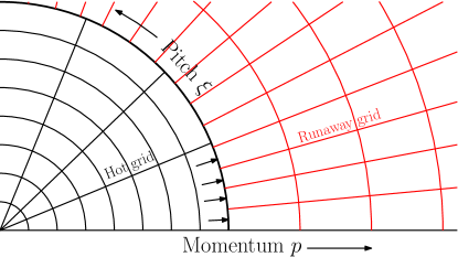
Figure 3: The hot (black) and runaway electron (red) kinetic grids are independent of each other but should allow for particles to flow freely between them.

5 Tests & benchmarks

A number of tests have been implemented for Dream in order to verify the correctness of both the individual modules in the code, and the overall physics modelled. For the latter, benchmarks against results in the published literature have been performed and in this section we present the results of three such benchmarks. The first two tests verify that the plasma conductivity and Dreicer runaway rates are accurately computed by comparing Dream simulations to simulations with the 2D Fokker–Planck solver Code [27, 28], and primarily validate the Fokker–Planck collision operator used. Code only simulates homogeneous plasmas, but uses the same test-particle collision operator as Dream, albeit with a finite difference discretization in momentum and a Legendre polynomial decomposition in pitch. The third test is to reproduce the tokamak disruption simulations in [13], which were carried out with the 1D fluid code Go [67, 49, 68].

5.1 Conductivity

A typical method for validating Fokker–Planck collision operators is to solve the Spitzer problem

$$eE_{\parallel}\frac{\partial f}{\partial p_{\parallel}}=C\left\{f\right\},$$ (73)

arising in the presence of a parallel electric field $E_{\parallel}$, where $C$ is the collision operator, including collisions between electrons and electrons, as well as electrons and ions. In the weak electric field limit ($E_{\parallel}\ll E_{\rm c}$, with $E_{\rm c}$ the critical electric field for runaway [3]) the current density $j$ carried by the distribution function $f$ will be proportional to $E_{\parallel}$, with constant of proportionality $\sigma$, i.e. the conductivity of the plasma at the given temperature and effective charge. By solving equation (73) for $f$, and by extension the current density $j$, we can obtain the plasma conductivity from the relation $\sigma=j/E_{\parallel}$.

In figure 4, the conductivity has been calculated with Dream (crosses) in the fully kinetic mode at a few different temperatures and plasma charges, and is compared to the conductivity as calculated with Code (solid lines). Both codes implement the fully relativistic test-particle collision operator of Ref. [69]. The values calculated with Dream are within less than $0.3\%$ of those calculated with Code, indicating that the collision operator is correctly implemented.

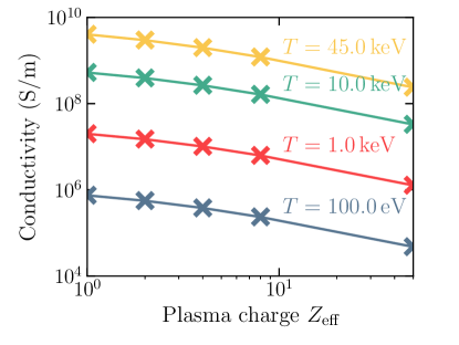
Figure 4: Comparison of plasma conductivity as calculated with Code (solid lines) and with Dream (crosses) at a few different temperatures $T$ and effective plasma charges $Z$. All calculated conductivities match to within $0.3\%$.

5.2 Runaway rate

Another quantity of importance to the physics studied in Dream is the so-called Dreicer runaway electron generation rate obtained in a $Z_{\rm eff}=1$ plasma when increasing $E_{\parallel}$ in the test above to $E_{\parallel}>E_{\rm c}$ [3]. In the fully kinetic mode, the number of runaway electrons $n_{\mathrm{re}}$ is then defined as the number of particles with momentum $p\geq p_{\mathrm{re}}$, where the runaway boundary is chosen as $p_{\mathrm{re}}=20\sqrt{2T/mc^{2}}$ with $T$ the electron temperature, and the runaway generation rate is taken as $\gamma=\partial n_{\mathrm{re}}/\partial t$. Figure 5 shows the primary runaway rate as calculated with Dream (crosses) and Code (circles). The solid lines are calculated with the formula given in [3]. The $x$ axis ranges from $E_{\parallel}=2E_{\rm c}$ to $E_{\parallel}=0.04E_{\rm D}$—where $E_{\rm D}$ denotes the Dreicer electric field [2] at which all electrons run away—corresponding to marginal and strong runaway electron generation respectively. The Dream and Code runaway rates match to within $3\%$.

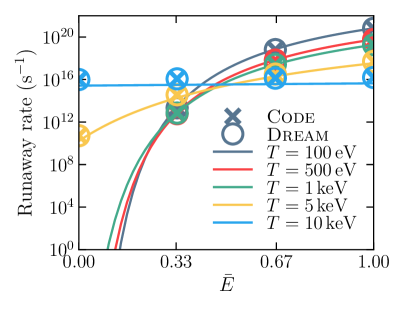
Figure 5: Comparison of the runaway rate as calculated with Code (circles), with Dream (crosses) and using the formula given in [3] (solid lines). The dimensionless variable $\bar{E}=(E-2E_{\rm c})/(0.04E_{\rm D}-2E_{\rm c})$ is introduced so that $\bar{E}\in[0,1]$ covers the region of $E$ in which the runaway generation is mild to modest, and the linearized collision operator is valid. The Code and Dream runaway rates match to within $3.5\%$.

5.3 GO ITER simulations

To validate the coupled physics of Dream  we will now present a comparison between Dream and the simulations of ITER-like disruptions conducted in [13]. In ref. [13] the effect of injecting impurities in the plasma on the maximum runaway current in a standard ITER scenario was studied using the 1D fluid code Go [67, 49, 68]. The Go code can be considered a predecessor of the fluid mode in Dream and uses similar models for the background plasma evolution. Using the fluid model, as described in section 2.2.3, with a cylindrical radial grid in Dream, the two codes should simulate approximately the same physics. While benchmarking the two codes it was discovered that some of the simulations in [13] were slightly under-resolved with respect to time. While it does not lead to any qualitative differences, for this comparison we have re-run the Go simulations with improved time resolution.

Figure 6 shows a comparison between the plasma currents and current densities obtained for cases 2, 3 and 4 in [13]. All three cases have the same temperature, main ion density and pre-disruption current density profiles, and only differ in the composition of the injected material. In all cases a mixture of neutral deuterium and neon is injected and is added instantaneously to the plasma, distributed uniformly across radii. The amount of material injected in the different cases is summarized in table 2.

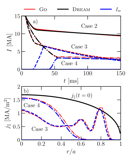
Figure 6: Comparison of (a) the time evolution of the total plasma current, and (b) maximum runaway current density profiles obtained with Dream (black/blue) and Go (red). In (a), the black curves show total plasma current, while blue curves show the runaway current component. In (b), the black curve indicates the initial current density profile.

Table 2: Amount of material injected in the ITER simulations described in section 5.3.

Case	Deuterium ($10^{20}\,${\mathrm{m}}^{-3}$$)	Neon ($10^{20}\,${\mathrm{m}}^{-3}$$)
Case 2	3	$0.03$
Case 3	40	$0.08$
Case 4	7	$0.08$

In all three cases considered, Dream closely reproduces both the total and runaway plasma currents in both the thermal and current quench phases of the disruptions, as well as the maximum runaway current density. The small deviations between the simulation results are explained primarily by the use of somewhat improved models for the critical electric field $E_{c}^{\rm eff}$ in Dream.

6 Comparison of electron models

To demonstrate some of the main features of Dream we will now examine two separate disruptions in a toroidal plasma with parameters representative of ASDEX Upgrade [70, 71, 72]. In section 6.1 we first describe the general parameters used for all simulations and briefly recall the differences between the electron models of Dream. Sections 6.2 and 6.3 then discuss the results and performance of each of the electron models.

6.1 Baseline simulation setup

All simulations of this section are conducted in an elongated ASDEX Upgrade-like plasma with magnetic field and vessel parameters as shown in table 3. Figure 7a shows the corresponding flux surfaces along with the plasma boundary (black) and conducting vessel wall structure (red). The flux surfaces are slightly elongated with a linearly varying elongation profile $\kappa(r)=1+0.15r/a$. In figure 7b-d radial profiles of the initial electron density, temperature and current density are shown. The electron density is nearly uniform, close to $n_{{\rm e},0}=$2.6\text{\times}{10}^{19}\text{\,}{\mathrm{m}}^{-3}$$, while the electron temperature is peaked at $T_{{\rm e},0}=$5.8\text{\,}\mathrm{keV}$$ on the magnetic axis and decreases towards $60\text{\,}\mathrm{e}\mathrm{V}$ near the edge. The plasma current density is $j(r)=j_{0}[1-(r/a)^{4}]^{3/2}$, with $j_{0}=$1.52\text{\,}\mathrm{M}\mathrm{A}\mathrm{/}\mathrm{m}\mathrm{{}^{2}}$$ chosen to give the desired total initial plasma current $I_{{\rm p},0}=$800\text{\,}\mathrm{k}\mathrm{A}$$.

Table 3: Magnetic field and vessel parameters used in the simulations of section 6.

Parameter	Value
Major radius $R_{\rm m}$	$1.65\text{\,}\mathrm{m}$
Minor radius $a$	$0.5\text{\,}\mathrm{m}$
Wall radius $b$	$0.55\text{\,}\mathrm{m}$
Elongation at edge $\kappa(a)$	$1.15$
Toroidal magnetic field $B_{0}$	$2.5\text{\,}\mathrm{T}$
Initial plasma current $I_{{\rm p},0}$	$800\text{\,}\mathrm{kA}$

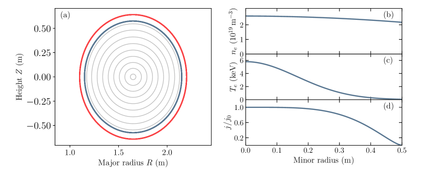
Figure 7: Parameters for the baseline scenario, which is used in all the simulations of section 6. (a) Magnetic field flux surfaces (gray), with the plasma boundary shown in blue and vessel wall in red. (b) Initial electron density. (c) Initial electron temperature. (d) Initial plasma current density profile, normalized to the central current density $j_{0}=$1.52\text{\,}\mathrm{MA}\text{\,}{\mathrm{m}}^{-2}$$.

In the following sections we will insert a combination of neutral deuterium and neutral argon into the plasma outlined above. The material is assumed to be instantly distributed uniformly across the plasma. Using four different electron models, we follow the evolution of the plasma using as it cools down due to radiation losses as well as a prescribed diffusive heat transport, according to (3.2), with $D_{W}=$4000\text{\,}\mathrm{m}^{2}\mathrm{/}\mathrm{s}$$ in section 6.2 and $D_{W}=$1000\text{\,}\mathrm{m}^{2}\mathrm{/}\mathrm{s}$$ in section 6.3. The four models used are the fully kinetic, the superthermal and the isotropic models described in section 2.2.2, as well as a fluid model similar to the one used in the Go code [13, 49, 50], which we briefly commented on in section 2.2.3. The main differences between these models can be briefly summarized as follows: in the fully kinetic model, both cold and hot electrons are modelled kinetically while runaway electrons are modelled as a fluid; in the superthermal model, only hot electrons are modelled kinetically, while cold and runaway electrons are modelled as fluids; the isotropic model makes the same assumptions as the superthermal model, but uses an angle-averaged kinetic equation and evolves only the energy distribution of the hot electrons; in the fluid model, only thermal bulk and runaway electron populations are followed, both as fluids.

Another important difference separating the fully kinetic/fluid and superthermal/isotropic models is the treatment of the cold electron temperature, $T_{\mathrm{cold}}$, which is used both in the test-particle collision operator and in the ion rate equations (41). In all models the temperature is evolved according to equation (3.2), and the electron distribution is initialized at equilibrium with the temperature of the hot initial plasma. In the fully kinetic and fluid models—which do not distinguish between cold and warm electrons—the temperature $T_{\mathrm{cold}}$ starts at the initial warm plasma temperature, and rapidly falls as cold impurities are inserted in the plasma. In contrast, in the superthermal and isotropic models, $T_{\mathrm{cold}}$ starts at almost zero, corresponding to the temperature of the injected impurities. The injected electrons will promptly form a Maxwellian at a significantly lower temperature than that of the pre-disruption plasma, and the hot electrons will predominantly slow down in free-free collisions with this cold Maxwellian. Because of these differences, the fully kinetic and fluid models can be expected to agree relatively well, while the superthermal and isotropic models could be expected to differ from the former two in some cases.

The cooling-down process occurring as impurities are injected into the hot plasma leads to an inherently non-linear evolution for the distribution function as it transitions from containing two Maxwellian electron populations—the injected electrons at a very low temperature and the initial bulk electrons at a warm, but gradually cooling, temperature—into a state dominated by a single Maxwellian electron population. The superthermal and isotropic models provide a numerically efficient way of capturing some of this dynamic without resorting to a fully non-linear collision operator.

Table 4: Typical wall clock times for the simulations conducted in section 6 on an Intel Xeon desktop computer with a total of $2\,800$ time steps.

Model	$N_{r}\times N_{\xi}\times N_{p}$	Wall time
Fluid	$15\times 1\times 1$	$25\text{\,}\mathrm{s}\mathrm{e}\mathrm{c}\mathrm{o}\mathrm{n}\mathrm{d}\mathrm{s}$
Isotropic	$15\times 1\times 80$	$1\text{\,}\mathrm{m}\mathrm{i}\mathrm{n}\mathrm{u}\mathrm{t}\mathrm{e}$ $40\text{\,}\mathrm{s}\mathrm{e}\mathrm{c}\mathrm{o}\mathrm{n}\mathrm{d}\mathrm{s}$
Superthermal	$15\times 68\times 80$	$1\text{\,}\mathrm{h}\mathrm{o}\mathrm{u}\mathrm{r}$ $7\text{\,}\mathrm{m}\mathrm{i}\mathrm{n}\mathrm{u}\mathrm{t}\mathrm{e}\mathrm{s}$
Fully kinetic	$15\times 68\times 140$	$4\text{\,}\mathrm{h}\mathrm{o}\mathrm{u}\mathrm{r}\mathrm{s}$

6.2 Full-conversion scenario

In this scenario we initiate the plasma as described in section 6.1 and insert neutral deuterium and argon with radially uniform densities $n_{\rm D}=n_{\rm Ar}=$2.6\text{\times}{10}^{19}\text{\,}{\mathrm{m}}^{-3}$$ at $t=0$. As shown in figure 8, the resulting temperature and current dynamics are very fast, with much of the thermal quench completing in about one hundred microseconds. Due to the rapid cooling, a significant fraction of electrons remain hot at the onset of the current quench, leading to a seamless conversion of ohmic current into superthermal and then runaway current via the hot-tail mechanism. By the end of the current quench, almost all of the original current has been converted into runaway current in all three models.

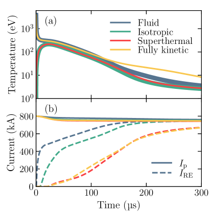
Figure 8: Time evolution of (a) cold electron temperature at $r/a=0.3$, (b) plasma current (solid) and runaway current (dashed) in the full-conversion scenario.

Some differences are observed in the evolution of the temperature and total runaway current in the fully kinetic/fluid and superthermal/isotropic models, although the total plasma current reached is almost exactly the same in all cases. Note that the temperature shown for the superthermal and isotropic models is that of the cold injected electrons, while the temperature shown for the fully kinetic and fluid models is that of the (initially warm) bulk electrons. The main reason for the differences in temperature evolution is the electron-ion heat exchange $Q_{ij}$ in equation (44), which explicitly depends on the relative temperature difference between electrons and ions. Since the initial value of $T_{\mathrm{cold}}$ differs in the four models, so does the heat transferred from the ions to the electrons, and hence also the detailed evolution of $T_{\mathrm{cold}}$. The fact that the runaway currents still agree well is due to the thermal quench being rapid in all models, which leads to the formation of a significant hot electron population that is eventually accelerated and runs away.

Figure 9 illustrates the evolution of the current carried by the distribution functions in the superthermal and fully kinetic models. In the former, the ohmic current is obtained from Ohm’s law (as in equation (28)) and the distribution function only carries superthermal current, while in the latter the distribution function also contains the thermal bulk electrons, and thus also carries ohmic current (seen as a sharp peak near $p=0$ in figure 9b). During the current quench, the remaining superthermal electrons—which carry a significant fraction of the total current—are accelerated to even higher momenta and run away. The absence of the thermal bulk in the superthermal model permits the momentum grid resolution to be nearly halved, making the superthermal model computationally efficient while accurate in capturing the hot-tail formation.

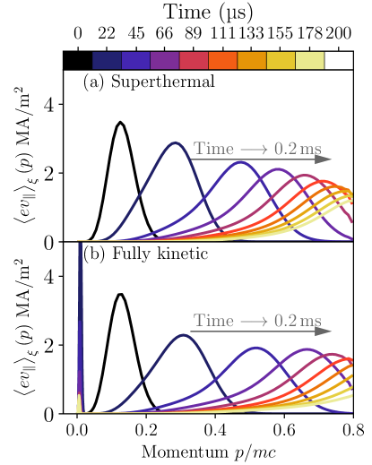
Figure 9: Time evolution of the $\xi$-averaged contribution to the parallel current from (a) the hot electron distribution function $f_{\rm hot}(r,p,\xi)$ in the superthermal model, and (b) from the electron distribution function $f(r,p,\xi)$ in the fully kinetic model. The latter contains both the ohmic (seen as a large peak near $p=0$) and the hot electron current.

6.3 Slow disruption scenario

In this scenario we initiate the plasma as described in section 6.1 and insert neutral deuterium and argon with radially uniform densities $n_{\rm D}=$5.2\text{\times}{10}^{20}\text{\,}{\mathrm{m}}^{-3}$$ and $n_{\rm Ar}=$5.2\text{\times}{10}^{18}\text{\,}{\mathrm{m}}^{-3}$$ respectively at $t=0$. The resulting disruption occurs over a relatively long time, with the current quench lasting for up to $4\text{\,}\mathrm{m}\mathrm{s}$, depending on the model used, as shown in figure 10b. As in section 6.2, the temperature shown in figure 10a for the superthermal and isotropic models is that of the cold injected electrons, while the temperature shown for the fully kinetic and fluid models is that of the (initially warm) bulk electrons. In contrast to the scenario of section 6.2, this scenario reveals significant differences between the different models used. The fluid and fully kinetic models mostly agree with each other, as do the isotropic and superthermal models, but when comparing the superthermal and fully kinetic models—the two most advanced models—the final runaway currents are found to deviate by a factor of two.

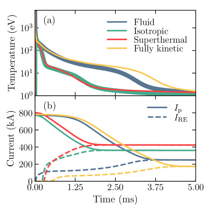
Figure 10: Time evolution of (a) cold electron temperature at $r/a=0.17$, (b) plasma current (solid) and runaway current (dashed) in the slow disruption scenario of section 6.3.

The deviations between the fluid/fully kinetic and isotropic/superthermal models in figure 10 are consequences of the self-consistent plasma evolution, although the origin of the different evolutions can be traced to the disparate definitions of the temperature used. Several terms and coefficients depend explicitly on the temperature $T_{\mathrm{cold}}$, including the ion rate coefficients in equation (41), the collisional energy transfer term (44), and the radial heat diffusion term, and as such, differing dynamics are to be expected in the brief initial phase of the TQ when $T_{\mathrm{cold}}$ differs significantly between the two groups of models. However, it is only if one or more of these temperature-dependent terms are dominant during the early TQ phase that the final runaway current should be significantly impacted. In the scenario of figure 10 it turns out that the radial heat diffusion term plays an important role in the fluid and fully kinetic models early during the TQ, causing the $T_{\mathrm{cold}}$ profile to be flattened. This in turn alters the behaviour of the electric field, which typically grows rapidly in response to the decreased conductivity when the temperature drops.

With the fluid and fully kinetic models, the relatively strong radial heat diffusion causes the temperature to decrease rapidly in the centre of the plasma, but also to be slightly raised at outer radii. As a result, the remaining thermal energy is radiated away more slowly, allowing the ohmic current to be maintained for a longer time, and thus delaying the increase of the electric field. Figure 11 shows the electric field evolution in the superthermal and fully kinetic models during this early phase of the disruption. The strong electric fields during the early phase of the disruption leads to a significant conversion of hot electrons to runaways. In the fully kinetic case, figure 11b, the slower electric field evolution does not allow for as many hot electrons to be immediately converted into runaways, but partially compensates for this later on during the disruption by driving more production of runaways through the avalanche mechanism. The increased avalanche generation in the fully kinetic model is however not sufficient to fully compensate for the early hot-tail generation in the superthermal model.

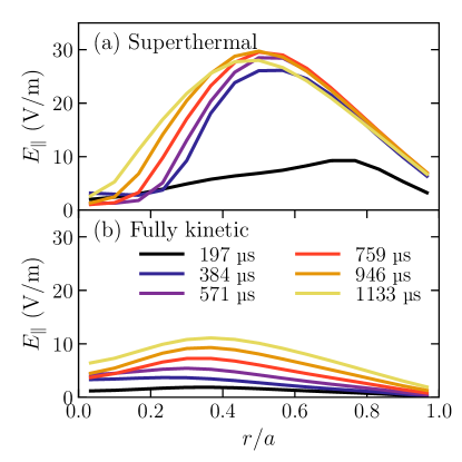
Figure 11: Electric field as a function of radius at a few times during the TQ phase in the scenario of section 6.3 using (a) the superthermal model, and (b) the fully kinetic model. The large difference in initial temperature between the models results in a significantly slower electric field evolution in the fully kinetic model.

The deviations between the fluid and fully kinetic models, as well as the isotropic and superthermal models, stem almost entirely from the differences in how the hot-tail generation is modelled. Both the fluid and isotropic models utilise approximations to the Fokker–Planck treatment of the hot-tail mechanism used in the superthermal and fully kinetic modes. As a result, the number of runaway electrons generated via the hot-tail mechanism is slightly over- and underestimated, respectively, in the fluid and isotropic modes.

Finally, a comment on the physics fidelity of the four considered models is due. The fluid and isotropic models are direct approximations of the more advanced models and are less reliable, although the results here suggest that their results for the temperature and current evolution are reasonably close to the more advanced kinetic models. As for the superthermal and fully kinetic models, it is difficult to clearly state that one is more reliable than the other. The fully kinetic model uses a linearized collision operator and in the early phase of the thermal quench, the process may be inherently non-linear. When a large amount of impurities are injected, the electron distribution will briefly be constituted by two Maxwellians at different temperatures, which the fully kinetic model is not equipped to handle. The superthermal model, on the other hand, is derived with this exact situation in mind and therefore provides a better approximation of the processes. The superthermal model is however still an approximation to the full disruption physics, and its assumptions, e.g. that a large number of impurities are present, are not necessarily always well satisfied. To verify the hot-tail models considered here, a relativistic non-linear collision operator, as used in Refs. [29, 73], coupled to a self-consistently evolving background plasma, is therefore needed. This will be considered in future work.

7 Summary

The main purpose of the Dream code is to model the self-consistent plasma evolution and runaway electron generation during a tokamak disruption. The output is the evolution of the temperature, densities of the different particle species and poloidal flux (which sets the evolution of the current density) as well as the electron distribution function. The temperature evolution includes ohmic heating, radiated power using atomic rate coefficients, collisional energy transfer from hot electrons and ions, as well as dilution cooling. The poloidal flux evolution includes the option to model rapid current flattening associated with fast magnetic reconnection events, via a helicity-conserving hyperresistivity term. The fluid quantities are solved on a one-dimensional flux-surface averaged grid, and the kinetic equation for the electron distribution is solved in a three-dimensional (1D-2P) bounce-averaged formulation.

The ability to treat electrons at various degrees of sophistication is one of the more novel contributions of Dream. The physics of tokamak disruptions typically involves multiple temporal and spatial scales, and so far often required comprehensive and computationally expensive simulations involving both fluid and full kinetic physics. By separating the electrons into cold, hot and runaway populations, and evolving the cold and runaway electrons using fluid models, Dream avoids resolving the usually uninteresting—but computationally intensive—kinetic bulk and runaway tail dynamics. Furthermore, the possibility to evolve hot electrons using a pitch angle-averaged kinetic equation allows simulation times to be reduced almost to the level of pure fluid models while the electron hot-tail generation is still accurately captured.

Together with the comprehensive physics model, which reaches beyond previous efforts in kinetic disruption modelling, the code is equipped with several attractive numerical features including fully implicit time stepping of the full system, as well as a flux conservative and positivity preserving discretization, which contributes to the robustness of the tool. Due to its flexibility and numerical efficiency, Dream is suitable for extensive investigations of disruption and runaway physics.

Dream has been verified against both kinetic and fluid codes, and has been found to reproduce their results in the appropriate limits. As an application, two disruption scenarios were investigated in an ASDEX Upgrade like tokamak, where the disruption is triggered by the injection of a combination of neutral deuterium and argon atoms. The full hierarchy of electron models was compared: fully kinetic, superthermal, isotropic and fluid models, and reasonable agreement was found. The difference in simulation time between the fluid and kinetic simulations is more than two orders of magnitude.

Appendix A Magnetic field and evaluation of flux surface integrals

In an axisymmetric tokamak of major radius $R_{\rm m}$, with ions uniformly distributed on the flux surfaces, the poloidal dependence of the coefficients of the transport equation (1) is naturally described in terms of three independent quantities $\eta_{1}=B/B_{\rm min}$, $\eta_{2}=R/R_{\rm m}$, $\eta_{3}=|\nabla r|^{2}$, as well as the pitch-angle dependent variable $\eta_{4}=\xi/\xi_{0}=\sqrt{[1-(1-\xi_{0}^{2})B/B_{\rm min}]/\xi_{0}^{2}}$. These have been introduced such that they all equal unity in a circular plasma, characterized by $R_{\rm m}=\infty$, which simplifies solutions in this limit. The minimum magnetic field on a flux surface has been denoted $B_{\rm min}(r)=\min(\sqrt{\boldsymbol{B}(r,\,\theta)^{2}}\,|\,\theta)$, with $r$ a flux surface label.

Flux surface integrals are efficiently carried out via

$$\int_{-\pi}^{\pi}X\,\mathrm{d}\theta\approx\sum_{i=1}^{N}w_{i}X(\theta_{i}),$$ (74)

evaluated with a Gauss-Legendre quadrature rule where the four independent angle-dependent quantities $\left\{\eta_{n}\right\}_{n=1}^{4}$ as well as the Jacobian $\mathcal{J}=1/|\nabla\varphi\cdot(\nabla r\times\nabla\theta)|$ are precomputed at the nodes $\theta_{i}$, where $N=10$ is found to typically be sufficient for relative errors $<10^{-4}$. For bounce integrals over trapped orbits, the integration limits $\theta_{b1}(\xi_{0})$ and $\theta_{b2}(\xi_{0})$ depend on pitch and the metric has an integrable singularity ($\sim 1/\sqrt{\theta_{b1,b2}^{2}-\theta^{2}}$) at the boundary, and a Chebyshev-Gauss quadrature is employed instead. In this case, the precomputed values must be separately evaluated on individual poloidal angle meshes for each trapped orbit, in contrast to passing orbits for which the same poloidal angle mesh can be reused.

The bounce-orbit metric $\mathcal{V}^{\prime}$ contains a logarithmic singularity on the trapped-passing boundary $\xi_{0}=\pm\xi_{T}$. In order to resolve these singular points, instead of using the midpoint rule to estimate the cell average in the finite-volume methods, for cells containing a singular point we instead carry out the pitch average

$$\oint X(\xi_{i},\,\theta)\,\mathrm{d}\theta\mapsto\frac{1}{\Delta\xi_{i}}\int_{\xi_{i-1/2}}^{\xi_{i+1/2}}\mathrm{d}\xi\oint\mathrm{d}\theta\,X(\xi,\,\theta)$$ (75)

as a double integral using the adaptive QAWS routine of QUADPACK, which is designed for integrals with endpoint singularities. For brevity, we have not written out other arguments on which the integrand may depend.

Dream supports the use of an analytic up-down symmetric geometry where the flux surfaces are parametrized according to

$$\boldsymbol{x} =R\hat{R}+z\hat{z},$$

$$R =R_{\rm m}+\Delta(r)+r\cos[\theta+\delta(r)\sin\theta],$$

$$z =r\kappa(r)\sin\theta,$$

$$\hat{R} =\cos\varphi\hat{x}+\sin\varphi\hat{y},$$

$$\boldsymbol{B} =G(r)\nabla\varphi+\frac{\psi_{\mathrm{ref}}^{\prime}(r)}{2\pi}\nabla\varphi\times\nabla r.$$ (76)

Here, the Shafranov shift $\Delta$, elongation $\kappa$ and triangularity $\delta$ parametrize the shape of the flux surfaces, and $G$ and the reference poloidal flux gradient $\psi_{\mathrm{ref}}^{\prime}$ (that is left independent of the poloidal flux $\psi$, evolved dynamically in the equation system) determine the strength of the toroidal and poloidal components of the magnetic field, respectively. In this geometry, the Jacobian $\mathcal{J}$ and scale factor $|\nabla r|^{2}$ are given by

$$\mathcal{J} =\kappa rR\biggl{\{}\cos(\delta\sin\theta)+\Delta^{\prime}\cos\theta+\sin\theta\sin[\theta+\delta\sin\theta]$$

$$\times\left[\frac{r\kappa^{\prime}}{\kappa}+\delta\cos\theta\left(1+\frac{r\kappa^{\prime}}{\kappa}-\frac{r\delta^{\prime}}{\delta}\right)\right]\biggr{\}},$$

$$|\nabla r|^{2} =\frac{\kappa^{2}r^{2}R^{2}}{\mathcal{J}^{2}}\Bigl{[}\frac{1}{\kappa^{2}}(1+\delta\cos\theta)^{2}\sin^{2}(\theta+\delta\sin\theta)$$

$$+\cos^{2}\theta\Bigr{]}.$$ (77)

Appendix B Kinetic equation

B.1 Heat transport due to fast-electron transport

The heat transport associated with the electron particle transport is obtained by integrating the diffusive transport term of the kinetic equation with the diffusion coefficient (23) over a Maxwell-Jüttner distribution function,

$$f_{M} =\frac{n_{\mathrm{cold}}}{4\pi\Theta K_{2}(1/\Theta)}e^{-\gamma/\Theta},$$

$$\frac{\partial f_{M}}{\partial r} =\frac{f_{M}}{T_{\mathrm{cold}}\Theta}\left(\gamma-3\Theta-\frac{K_{1}(1/\Theta)}{K_{2}(1/\Theta)}\right)\frac{\partial T_{\mathrm{cold}}}{\partial r},$$ (78)

$$\Theta =\frac{T_{\mathrm{cold}}}{m_{e}c^{2}},$$ (79)

where we do not keep the contribution from $\partial n_{\mathrm{cold}}/\partial r$ since electron density cannot be transported independently of the ions; the electron density profile is set by quasineutrality. As such, we assume that the heat transport acts to flatten the temperature profile. Therefore, the heat diffusion coefficient is given by the energy moment ($m_{e}c^{2}(\gamma-1)$)

$$D_{W} =\frac{2}{3n_{\mathrm{cold}}}\int_{0}^{\infty}\mathrm{d}p\,\frac{f_{M}}{\Theta^{2}}(\gamma-1)$$

$$\times\left(\gamma-3\Theta-\frac{K_{1}(1/\Theta)}{K_{2}(1/\Theta)}\right)\int_{-1}^{1}\mathrm{d}\xi_{0}\,\frac{\mathcal{V}^{\prime}}{V^{\prime}}\left\{D^{rr}\right\}.$$ (80)

For the Rechester-Rosenbluth model (23) the pitch integral is given by

$$\int_{-1}^{1}\mathrm{d}\xi_{0}\,\frac{\mathcal{V}^{\prime}}{V^{\prime}}\left\{D^{rr}\right\}=2\pi p^{2}v\left\langle\frac{B}{B_{\mathrm{max}}}\right\rangle\pi qR_{\rm m}c\left(\frac{\delta B}{B}\right)^{2},$$ (81)

yielding

$$D_{W} =\frac{2}{3}\left\langle\frac{B}{B_{\mathrm{max}}}\right\rangle\pi qR_{\rm m}c\left(\frac{\delta B}{B}\right)^{2}\frac{1}{e^{1/\Theta}K_{2}(1/\Theta)}$$

$$\times\left[(2+3\Theta)\left(1-\frac{K_{1}}{K_{2}}\right)+3\Theta^{2}\right]$$ (82)

$$\approx\frac{2\pi}{3}qR_{\rm m}c\left(\frac{\delta B}{B}\right)^{2}\sqrt{\frac{18\Theta}{\pi}}\left[1-\frac{5}{8}\Theta\right]\left\langle\frac{B}{B_{\mathrm{max}}}\right\rangle,$$

with the last line corresponding to the non-relativistic limit $\Theta\ll 1$, retaining the leading-order relativistic correction.

B.2 Reduced kinetic equation

For the isotropic electron mode, described in section 2.2.2, a reduced form of the usual kinetic equation detailed in section 2.1 is used, analogous to Ref. [8]. To derive the reduced equation, we first introduce the ordering parameter $\delta$ and assume $\nu_{D}\sim\delta^{0}$ and $E\sim\delta^{1}$, with all other terms being of order $\delta^{2}$. Writing $f=f_{0}+\delta f_{1}+\mathcal{O}(\delta^{2})$ and grouping the kinetic equation by order in $\delta$, we obtain a set of new equations governing the evolution of the distribution function:

$$\delta^{0}:\quad\frac{\partial}{\partial\xi_{0}}\left[\mathcal{V}^{\prime}\left\{\frac{\xi^{2}}{\xi_{0}^{2}}\frac{B_{\mathrm{min}}}{B}\right\}\left(1-\xi_{0}^{2}\right)\frac{\partial f_{0}}{\partial\xi_{0}}\right]=0$$ (83a)

$$\begin{gathered}\delta^{1}:\quad e\left\{E_{\parallel}\xi\right\}\left[\frac{1}{p^{2}}\frac{\partial}{\partial p}\left(p^{2}f_{0}\right)+\frac{1}{p\xi_{0}}\frac{\partial}{\partial\xi_{0}}\left[\left(1-\xi_{0}^{2}\right)f_{0}\right]\right]=\\ =\frac{\nu_{D}}{2\mathcal{V}^{\prime}}\frac{\partial}{\partial\xi_{0}}\left[\mathcal{V}^{\prime}\left\{\frac{\xi^{2}}{\xi_{0}^{2}}\frac{B_{\mathrm{min}}}{B}\right\}\left(1-\xi_{0}^{2}\right)\frac{\partial f_{1}}{\partial\xi_{0}}\right]\end{gathered}$$ (83b)

$$\begin{gathered}\delta^{2}:\quad\frac{\partial f_{0}}{\partial t}=\frac{1}{\mathcal{V}^{\prime}}\frac{\partial}{\partial p}\biggl{[}\mathcal{V}^{\prime}\biggl{(}-\left\{\hat{A}^{p}\right\}f_{0}\\ -e\left\{E_{\parallel}\xi\right\}f_{1}+\left\{D^{pp}\right\}\frac{\partial f_{0}}{\partial p}\biggr{)}\biggr{]}+\frac{1}{\mathcal{V}^{\prime}}\frac{\partial\mathcal{V}^{\prime}F^{\xi_{0}}}{\partial\xi_{0}}\\ +\frac{1}{\mathcal{V}^{\prime}}\frac{\partial}{\partial r}\left[\mathcal{V}^{\prime}\left(-\left\{A^{r}\right\}f_{0}+\left\{D^{rr}\right\}\frac{\partial f_{0}}{\partial r}\right)\right]+\left\{S\right\},\end{gathered}$$ (83c)

where in the last equation, $\hat{A}^{p}$ denotes the momentum advection that is not due to electric-field acceleration, and $F^{\xi_{0}}$ denotes the net pitch flux, which will not affect the final result. Solving the $\delta^{0}$ equation (83a) first yields the leading order solution

$$f_{0}=f_{0}\left(t,r,p\right),$$ (84)

i.e. $f_{0}$ is isotropic. Substituting this into the next order equation (83b) and integrating the result over $\xi_{0}$ from $-1$ to $\xi_{0}$ yields

$$-\pi h\left(\xi_{0}\right)p^{2} V^{\prime}\frac{e\left\langle\boldsymbol{E}\cdot\boldsymbol{B}\right\rangle}{\nu_{D}B_{\mathrm{min}}}\frac{\partial f_{0}}{\partial p}=$$ (85)

$$\mathcal{V}^{\prime}\left\{\frac{\xi^{2}}{\xi_{0}^{2}}\frac{B_{\mathrm{min}}}{B}\right\}\left(1-\xi_{0}^{2}\right)\frac{\partial f_{1}}{\partial\xi_{0}},$$

with the function

$$h\left(\xi_{0}\right) =2\int_{\xi_{0}}^{1}\mathrm{d}\xi_{0}\,\xi_{0}\mathcal{H}(\xi_{0})$$ (86)

$$=\begin{cases}1-\xi_{T}^{2},&\text{trapped},\\ 1-\xi_{0}^{2},&\text{passing},\end{cases}$$

where the step function $\mathcal{H}$ was defined in (24). A solution for $f_{1}$ can then be obtained by isolating $\partial f_{1}/\partial\xi_{0}$ and integrating over $\xi_{0}$ once more, giving

$$\begin{gathered}f_{1}\left(t,r,p,\xi_{0}\right)=-\pi p^{2}\frac{eV^{\prime}\left\langle\boldsymbol{E}\cdot\boldsymbol{B}\right\rangle}{\nu_{D}B_{\mathrm{min}}}\frac{\partial f_{0}}{\partial p}\times\\ \times\int_{-1}^{\xi_{0}}\frac{h\left(\xi_{0}^{\prime}\right)\,\mathrm{d}\xi_{0}^{\prime}}{\mathcal{V}^{\prime}\left\{\xi^{2}B_{\mathrm{min}}^{2}/(\xi_{0}^{2}B^{2})\right\}\left(1-\xi_{0}^{\prime 2}\right)}.\end{gathered}$$ (87)

With $f_{0}$ and $f_{1}$ determined, we may now use the $\delta^{2}$ equation (83c) to obtain the final reduced kinetic equation. We first multiply both sides of equation (83c) by $\mathcal{V}^{\prime}$ and integrate over all $\xi_{0}$. Because of this, the pitch angle scattering term, as well as the $\xi_{0}$ component of the electric field term, vanish due to the factors of $1-\xi_{0}^{2}$ which are zero at $\xi_{0}=\pm 1$. The slowing down and transient terms remain mostly unaffected by the integration, only picking up a factor of

$$\begin{gathered}\int_{-1}^{1}\mathrm{d}\xi_{0}\,\mathcal{V}^{\prime}=2\pi\int_{0}^{2\pi}\mathrm{d}\phi\int_{-1}^{1}\mathrm{d}\xi_{0}\oint\mathrm{d}\theta\,\sqrt{g}=\\ =2\pi\int_{0}^{2\pi}\mathrm{d}\phi\int_{0}^{2\pi}\mathrm{d}\theta\left(\int_{-1}^{-\xi_{T}}+\int_{\xi_{T}}^{1}\right)\mathrm{d}\xi_{0}\,\sqrt{g}=\\ =2\pi p^{2}\int_{0}^{2\pi}\mathrm{d}\phi\int_{0}^{2\pi}\mathrm{d}\theta\,\mathcal{J}\times\\ \times\left(\int_{-1}^{-\xi_{T}}+\int_{\xi_{T}}^{1}\right)\frac{B}{B_{\mathrm{min}}}\frac{\xi_{0}}{\xi}\,\mathrm{d}\xi_{0}=4\pi p^{2}V^{\prime},\end{gathered}$$ (88)

while the electric field term becomes

$$\begin{gathered}2\pi\frac{V^{\prime}e\left\langle\boldsymbol{E}\cdot\boldsymbol{B}\right\rangle}{B_{\mathrm{min}}}\frac{\partial}{\partial p}\int_{-1}^{1}\mathrm{d}\xi_{0}\,p^{2}\xi_{0}f_{1}\mathcal{H}\left(\xi_{0}\right)=\\ =-\pi\frac{V^{\prime}\left(e\left\langle\boldsymbol{E}\cdot\boldsymbol{B}\right\rangle\right)^{2}}{B_{\mathrm{min}}^{2}}\frac{\partial}{\partial p}\int_{-1}^{1}\mathrm{d}\xi_{0}\,\frac{p^{2}\xi_{0}}{\nu_{D}}\mathcal{H}\left(\xi_{0}\right)\times\\ \times\int_{-1}^{\xi_{0}}\frac{-h\left(\xi_{0}^{\prime}\right)\mathrm{d}\xi_{0}^{\prime}}{\left\langle\xi/\xi_{0}^{\prime}\right\rangle\left(1-\xi_{0}^{\prime 2}\right)}\end{gathered}$$ (89)

where the expression (87) for $f_{1}$ was substituted. After interchanging the order of integration, the $\xi_{0}^{\prime}$ integral ranges over the passing region only due to the step function, while the $\xi_{0}$ integral is recognized as half the function $h(\xi_{0}^{\prime})$. Since we will then only evaluate $h(\xi_{0}^{\prime})$ in the passing region, we may replace it by its actual value there, $h(\xi_{0}^{\prime}\in\text{passing})=1-\xi_{0}^{\prime 2}$. Furthermore, since the integrand is even in $\xi_{0}^{\prime}$ in the passing region, we may replace the integral with two times the integral ranging from $\xi_{T}$ to $1$:

$$\begin{gathered}\eqref{eq:app:kineq:Eterm}=-\pi\frac{V^{\prime}\left(e\left\langle\boldsymbol{E}\cdot\boldsymbol{B}\right\rangle\right)^{2}}{B_{\mathrm{min}}^{2}}\int_{\xi_{T}}^{1}\frac{1-\xi_{0}^{\prime 2}}{\left\langle\xi/\xi_{0}^{\prime}\right\rangle}\,\mathrm{d}\xi_{0}^{\prime}\times\\ \times\frac{\partial}{\partial p}\left(\frac{p^{2}}{\nu_{D}}\frac{\partial f_{0}}{\partial p}\right).\end{gathered}$$ (90)

The electric field term, which was purely advective in the original kinetic equation, has now become purely diffusive after the averaging procedure.

For the radial transport terms the $\xi_{0}$ integral will only apply to the advection and diffusion coefficients, and so we can make use of the relation

$$\int_{-1}^{1}\mathrm{d}\xi_{0}\,\mathcal{V}^{\prime}\left\{X\right\} =\int_{-1}^{1}\mathrm{d}\xi_{0}\,\mathcal{V}^{\prime}\frac{2\pi}{\mathcal{V}^{\prime}}\int_{0}^{2\pi}\mathrm{d}\phi\oint\mathrm{d}\theta\sqrt{g}X=$$ (91)

$$=2\pi\int_{0}^{2\pi}\mathrm{d}\phi\int_{-1}^{1}\mathrm{d}\xi_{0}\oint\sqrt{g}X=$$

$$=2\pi p^{2}\int_{0}^{2\pi}\mathrm{d}\phi\int_{0}^{2\pi}\mathrm{d}\theta\int_{-1}^{1}\mathrm{d}\xi\,X=$$

$$=4\pi p^{2}\left\langle\frac{1}{2}\int_{-1}^{1}\mathrm{d}\xi\,X\right\rangle\equiv 4\pi p^{2}\left\langle X\right\rangle_{\xi},$$

where in the next-to-last step we used that $B_{\mathrm{min}}\xi\,\mathrm{d}\xi=B\xi_{0}\,\mathrm{d}\xi_{0}$. In what remains, we will use the notation $\left\langle X\right\rangle_{\xi}$ to denote the combined flux surface and pitch average of a quantity $X$.

After the steps above, we obtain the final reduced kinetic equation by dividing all terms by $\int\mathcal{V}^{\prime}\mathrm{d}\xi_{0}=4\pi p^{2}V^{\prime}$, yielding

$$\begin{gathered}\frac{\partial f_{0}}{\partial t}=\frac{1}{p^{2}}\frac{\partial}{\partial p}\biggl{[}p^{2}\biggl{(}-\left\langle\hat{A}^{p}\right\rangle_{\xi}f_{0}+\left(\left\langle D^{pp}\right\rangle_{\xi}+\mathcal{D}_{E}\right)\frac{\partial f_{0}}{\partial p}\biggr{)}\biggr{]}\\ +\frac{1}{V^{\prime}}\frac{\partial}{\partial r}\left[V^{\prime}\left(-\left\langle A^{r}\right\rangle_{\xi}f_{0}+\left\langle D^{rr}\right\rangle_{\xi}\frac{\partial f_{0}}{\partial r}\right)\right]+\left\langle S\right\rangle_{\xi},\\ \mathcal{D}_{E}=f_{\rm p}\frac{(e\left\langle\boldsymbol{E}\cdot\boldsymbol{B}\right\rangle)^{2}}{3\left\langle B^{2}\right\rangle\nu_{D}(p)}.\end{gathered}$$ (92)

Here we have introduced $\mathcal{D}_{E}$ as the momentum diffusion coefficient representing the electric-field acceleration, and the effective passing fraction, denoted $f_{\rm p}$, is defined as

$$f_{\rm p}=\frac{3}{4}\left\langle\frac{B^{2}}{B_{\mathrm{min}}^{2}}\right\rangle\int_{\xi_{T}}^{1}\frac{1-\xi_{0}^{\prime 2}}{\left\langle\xi/\xi_{0}^{\prime}\right\rangle}\,\mathrm{d}\xi_{0}^{\prime}.$$ (93)

Current density

The current density corresponding to the distribution evolved by the reduced kinetic equation can be calculated from equation (32). Since $f_{0}$ is isotropic, $f_{1}$ is the lowest-order component of $f$ to carry any current, and the current density therefore becomes

$$\begin{gathered}\frac{j_{\rm iso}}{B}=\pi e^{2}\frac{\left\langle\boldsymbol{E}\cdot\boldsymbol{B}\right\rangle}{B_{\mathrm{min}}^{2}}\int\mathrm{d}p\mathrm{d}\xi_{0}\,\frac{vp^{2}}{\nu_{D}}\mathcal{H}\left(\xi_{0}\right)\xi_{0}\frac{\partial f_{0}}{\partial p}\times\\ \times\int_{-1}^{\xi_{0}}\frac{h\left(\xi_{0}^{\prime}\right)\mathrm{d}\xi_{0}^{\prime}}{\left\langle\xi/\xi_{0}^{\prime}\right\rangle\left(1-\xi_{0}^{2}\right)}.\end{gathered}$$ (94)

Just as for the electric field term, we interchange the order of integration in $\xi_{0}$ and $\xi_{0}^{\prime}$ and recognize that the $\xi_{0}$ integral yields a factor of $(1/2)h(\xi_{0}^{\prime})$. The current density is hence given by

$$\frac{j_{\rm iso}}{B}=\frac{2\pi e^{2}f_{\rm p}}{3}\frac{\left\langle\boldsymbol{E}\cdot\boldsymbol{B}\right\rangle}{\left\langle B^{2}\right\rangle}\int\mathrm{d}p\frac{vp^{2}}{\nu_{D}}\frac{\partial f_{0}}{\partial p}.$$ (95)

An undesirable property of (95) is that it allows for the current density to grow larger than $ecn_{e}$, which is the current density expected when all electrons travel at the speed of light along magnetic field lines. Exceeding this value may destabilize the solver, and so we adjust for this behaviour by smoothly matching the limit of all electrons travelling parallel to magnetic field lines, in which case the current density is given by

$$\frac{j_{\rm iso,2}}{B}=4\pi e\,\mathrm{sgn}(\left\langle\boldsymbol{E}\cdot\boldsymbol{B}\right\rangle)\int\mathrm{d}p\,vp^{2}f,$$ (96)

where $\mathrm{sgn}(x)$ denotes the sign function. The actual current density used in the simulation is then taken as the matched formula

$$j=\frac{j_{\rm iso}j_{\rm iso,2}}{\sqrt{j_{\rm iso}^{2}+j_{\rm iso,2}^{2}}},$$ (97)

corresponding approximately to the smallest of the two approximations.

Appendix C Runaway fluid formulae in general tokamak geometry

A widely used formula for the avalanche growth rate in a pure plasma was derived by Rosenbluth & Putvinski [8], accounting for geometric effects in a large-aspect-ratio tokamak. This formula has later been generalized to partially ionized plasmas [74, 75], which has also been applied to runaway generation due to Compton scattering and tritium beta decay [48, 13]. Here, we present generalized fluid formulae for the runaway generation rate that extends the validity of previous work to axisymmetric tokamak geometry with shaped surfaces of arbitrary aspect ratio.

C.1 Analytic runaway rate from source function $S$

Runaway production mechanisms other than Dreicer and hot-tail generation—such as large-angle collisions, beta decay of tritium and Compton scattering—are typically modelled by a source function defined in the particle phase space $S=S(t,\,\boldsymbol{x},\,\boldsymbol{p})$. A general procedure for deriving the corresponding fluid runaway rate from such a source function follows from the ordering made in B.2 in the superthermal limit, where $D^{pp}$ is negligible. We also assume runaway formation to occur in quasi-steady state and that radial transport occurs on longer time scales, by ordering $\partial/\partial t\sim A^{r}\sim D^{rr}\sim\delta^{3}$. Doing so casts the second-order equation (83c) into the form

$$\frac{1}{p^{2}}\frac{\partial}{\partial p}\left[p^{2}\left(\left\langle A^{p}\right\rangle_{\xi}f+\mathcal{D}_{E}\frac{\partial f}{\partial p}\right)\right]+\left\langle S\right\rangle_{\xi}=0,$$ (98)

In the steady-state fluid picture, since $\langle A^{p}\rangle_{\xi}$ and $\mathcal{D}_{E}$ become constant in the limit $v\to c$, the rate at which new runaway electrons are generated can be defined as the particle flux to $p=\infty$,

$$\frac{\partial\left\langle n_{\mathrm{re}}\right\rangle}{\partial t}=-4\pi p^{2}\left(\left\langle A^{p}\right\rangle_{\xi}f+\mathcal{D}_{E}\frac{\partial f}{\partial p}\right)_{p=\infty}.$$ (99)

Note that the purpose of the source function $S$ in (98) is to create new free electrons at any energy, not necessarily runaway electrons. For a newly created electron to become a runaway, it must be successfully accelerated into the runaway region, and the probability for this is determined by the advective and diffusive processes dominating the electron dynamics. By integrating equation (98) from $p$ to $\infty$ we obtain a relation between the runaway generation rate, the source term $S$ and the advection-diffusion processes determining the probability for runaway:

$$\begin{gathered}p^{2}\left(\left\langle A^{p}\right\rangle_{\xi}f+\mathcal{D}_{E}\frac{\partial f}{\partial p}\right)=\\ -\frac{1}{4\pi}\frac{\partial\left\langle n_{\mathrm{re}}\right\rangle}{\partial t}+\int_{p}^{\infty}\mathrm{d}p^{\prime}\,p^{\prime 2}\left\langle S(p^{\prime})\right\rangle_{\xi}.\end{gathered}$$ (100)

To solve this equation for the runaway generation rate, we introduce the integrating factor

$$G=-\int_{p}^{\infty}\frac{\left\langle A^{p}\right\rangle_{\xi}(p^{\prime})}{\mathcal{D}_{E}(p^{\prime})}\,\mathrm{d}p^{\prime},$$ (101)

and divide equation (100) by $p^{2}D^{pp}$ to obtain

$$\frac{\partial\mathrm{e}^{G}f}{\partial p}=\frac{\mathrm{e}^{G}}{p^{2}D_{E}}\left(-\frac{1}{4\pi}\frac{\partial\left\langle n_{\mathrm{re}}\right\rangle}{\partial t}+\int_{p}^{\infty}\mathrm{d}p^{\prime}\,p^{\prime 2}\left\langle S\right\rangle_{\xi}\left(p^{\prime}\right)\right).$$ (102)

If we assume that $f$ is well-behaved, so that $\mathrm{e}^{G}f|_{p=\infty}=\mathrm{e}^{G}f|_{p=0}=0$, where the latter follows from the fact that $\lim_{p\to 0}G=-\infty$, we can integrate (102) over all momenta:

$$\begin{gathered}\frac{1}{4\pi}\frac{\partial\left\langle n_{\mathrm{re}}\right\rangle}{\partial t}\int_{0}^{\infty}\mathrm{d}p\frac{\mathrm{e}^{G}}{p^{2}\mathcal{D}_{E}}=\\ =\int_{0}^{\infty}\mathrm{d}p\frac{\mathrm{e}^{G}}{p^{2}\mathcal{D}_{E}}\int_{p}^{\infty}\mathrm{d}p^{\prime}\,p^{\prime 2}\left\langle S\right\rangle_{\xi}\left(p^{\prime}\right)=\\ =\int_{0}^{\infty}\mathrm{d}p\,p^{2}\left\langle S\right\rangle_{\xi}\left(p\right)\int_{0}^{p}\mathrm{d}p^{\prime}\,\frac{\mathrm{e}^{G\left(p^{\prime}\right)}}{p^{\prime 2}\mathcal{D}_{E}\left(p^{\prime}\right)}\end{gathered}$$ (103)

Solving for $\partial\left\langle n_{\mathrm{re}}\right\rangle/\partial t$ then yields

$$\begin{gathered}\frac{\partial\left\langle n_{\mathrm{re}}\right\rangle}{\partial t}=4\pi\int_{0}^{\infty}\mathrm{d}p\,p^{2}\left\langle S\right\rangle_{\xi}\left(p\right)h\left(p\right)\\ =\left\langle\int h(p)S(t,\boldsymbol{x},\boldsymbol{p})\,\mathrm{d}\boldsymbol{p}\right\rangle,\end{gathered}$$ (104)

where

$$h\left(p\right)=\frac{\int_{0}^{p}\mathrm{d}p^{\prime}\frac{\mathrm{e}^{G}}{p^{\prime 2}\mathcal{D}_{E}}}{\int_{0}^{\infty}\mathrm{d}p^{\prime}\frac{\mathrm{e}^{G}}{p^{\prime 2}\mathcal{D}_{E}}}$$ (105)

can be interpreted as the probability for an electron created with momentum $p$ to run away. In the non-relativistic limit, for a fully ionized plasma with constant Coulomb logarithm, $\left\langle A^{p}\right\rangle_{\xi}$ is proportional to $1/p^{2}$, allowing an exact integration of the runaway probability

$$h(p)=e^{G}=\exp\left[-\frac{3}{4}\frac{\left\langle B^{2}\right\rangle p^{2}\nu_{s}\nu_{D}}{f_{\rm p}(e\left\langle\boldsymbol{E}\cdot\boldsymbol{B}\right\rangle)^{2}}\right]$$ (106)

Since the exponent varies rapidly with momentum, $p^{2}\nu_{s}\nu_{D}\propto 1/p^{4}$, the runaway probability $h$ is well approximated by a step function at the critical momentum $p_{\star}$ defined by

$$\begin{gathered}p_{\star}^{2}\nu_{s}(p_{\star})\nu_{D}(p_{\star})=f_{\rm p}\frac{(e\left\langle\boldsymbol{E}\cdot\boldsymbol{B}\right\rangle)^{2}}{\left\langle B^{2}\right\rangle}.\end{gathered}$$ (107)

The validity of the runaway rates can be extended to the near-threshold regime $E\sim E_{c}$ and to weak pitch scattering $\nu_{D}\sim 0$ by defining a matched formula for the critical runaway momentum $p_{c}$ according to [75]

$$p_{c}=\left(\frac{\bar{\nu}_{s}(p_{\star})\bar{\nu}_{D}(p_{\star})+4\bar{\nu}_{s}(p_{\star})^{2}}{f_{\rm p}e^{2}({\left\langle\boldsymbol{E}\cdot\boldsymbol{B}\right\rangle}/{\sqrt{\left\langle B^{2}\right\rangle}}-E_{\rm c}^{\rm eff})^{2}}\right)^{1/4},$$ (108)

where $\bar{\nu}_{s}=p^{3}\nu_{s}/\gamma^{2}$ and $\bar{\nu}_{D}=p^{3}\nu_{D}/\gamma$ denote normalized collision frequencies that depend only weakly on momentum. In this expression $E_{\rm c}^{\rm eff}$ denotes the effective critical field, described in C.2, and $p_{c}=\infty$ when the electric field is smaller than $E_{\rm c}^{\rm eff}$. Compared to ref. [75], the numerator includes a factor of $\bar{\nu}_{s}^{2}$ which increases the accuracy of the formula for weakly ionized low-$Z$ plasmas. In Dream, the runaway rate due to source functions are evaluated using equation (104) with the runaway probability

$$h(p)=H(p-p_{c}),$$ (109)

where $H$ denotes the Heaviside step function. The source function $S$ due to Compton and tritium decay are modelled as in ref. [13].

C.2 Evaluation of critical electric field

The critical electric field for runaway generation is the weakest electric field required for net acceleration of any electron in the plasma to occur. The original expression for this field, derived by Connor and Hastie [3], only considered electric field acceleration and deceleration due to collisional friction. However, it has been experimentally observed that the actual, or effective, critical electric field is likely larger than the value given by Connor and Hastie. Several theoretical studies have since generalized original Connor and Hastie expression to also account for the effect of bremsstrahlung and synchrotron radiation, as well as the partial ionization of atoms. In Dream, we use the method described in [76], further generalized to tokamak geometry. Below, we derive the equation which must be minimized to obtain the effective critical electric field and describe how it is implemented in a computationally efficient manner.

Theory

Following ref. [76], we consider the kinetic equation

$$\frac{\partial f}{\partial t} =-\frac{1}{\mathcal{V}^{\prime}}\frac{\partial}{\partial p}\left(\mathcal{V}^{\prime}\left\{A^{p}\right\}f\right)$$ (110)

$$+\frac{1}{\mathcal{V}^{\prime}}\frac{\partial}{\partial\xi_{0}}\left[\mathcal{V}^{\prime}\left(-\left\{A^{\xi_{0}}\right\}f+\left\{D^{\xi_{0}\xi_{0}}\right\}\frac{\partial f}{\partial\xi_{0}}\right)\right],$$

where the bounce-averaged advection-diffusion coefficients $\{A^{p}\}$, $\{A^{\xi_{0}}\}$ and $\{D^{\xi_{0}\xi_{0}}\}$ contain the effects of electric field acceleration, partial ionization and radiation losses (bremsstrahlung and synchrotron) as described in B. Near the critical momentum for runaway acceleration it is expected that pitch fluxes dominate over energy fluxes, i.e. $\{A^{\xi_{0}}\}\sim\{D^{\xi_{0}\xi_{0}}\}\gg\{A^{p}\}$, allowing us to obtain an expression for the steady-state pitch distribution

$$\begin{gathered}0=-\left\{A^{\xi_{0}}\right\}f+\left\{D^{\xi_{0}\xi_{0}}\right\}\frac{\partial f}{\partial\xi_{0}},\\ \implies f\left(\xi_{0}\right)\propto\exp\left[-\int_{\xi_{0}}^{1}\frac{\left\{A^{\xi_{0}}\right\}}{\left\{D^{\xi_{0}\xi_{0}}\right\}}\,\mathrm{d}\xi_{0}^{\prime}\right].\end{gathered}$$ (111)

The exponent in the expression for $f$ can be written in the form

$$\frac{\left\{A^{\xi_{0}}\right\}}{\left\{D^{\xi_{0}\xi_{0}}\right\}}=Ag\left(\xi_{0}\right),$$ (112)

where in the cylindrical theory $A=2eE/(p\nu_{D})$ and $g=1-\xi_{0}$. In the general case, we have

$$A =\frac{2e\left\langle\boldsymbol{E}\cdot\boldsymbol{B}\right\rangle}{p\nu_{D}B_{\rm min}},$$

$$g =\begin{cases}H\left(\xi_{0},1\right),&\quad\xi_{T}<\xi_{0}\leq 1\\ H\left(\xi_{T},1\right),&\quad-\xi_{T}\leq\xi_{0}\leq\xi_{T}\\ H\left(\xi_{T},1\right)+H\left(\xi_{0},-\xi_{T}\right),&\quad-1\leq\xi_{0}<-\xi_{T}\end{cases}$$

with the auxiliary function

$$H\left(\xi_{1},\xi_{2}\right)=\int_{\xi_{1}}^{\xi_{2}}\frac{\xi_{0}}{\left\langle\xi\right\rangle}\mathrm{d}\xi_{0}.$$ (113)

Next, after substituting (111) back into the kinetic equation (110), the kinetic equation is integrated over $\mathrm{d}\xi_{0}\mathcal{V}^{\prime}/V^{\prime}$ to yield

$$\frac{\partial F_{0}}{\partial t}+\frac{\partial\left(U(p)F_{0}\right)}{\partial p}=0,$$ (114)

where the distribution-weighted bounce averaged momentum flux—or net acceleration—$U(p)$ is

$$U(p)=\frac{\int\mathcal{V}^{\prime}\left\{A^{p}\right\}f\,\mathrm{d}\xi_{0}}{\int\mathcal{V}^{\prime}f\,\mathrm{d}\xi_{0}}.$$ (115)

The effective critical electric field $E_{c}^{\rm eff}$ is then defined as the minimum value of the electric field for which there exists a real solution to $U(p)=0$, that is

$$E_{c}^{\rm eff}=\min\left(\left.\frac{\left\langle\boldsymbol{E}\cdot\boldsymbol{B}\right\rangle}{\sqrt{\left\langle B^{2}\right\rangle}}\right|U(p)=0\right).$$ (116)

Implementation

The calculation of $U(p)$ typically requires repeated evaluation of three nested integrals, two of which stand inside an exponential function, and is hence not entirely straightforward to implement efficiently. To speed up evaluation we use splines to evaluate the function $g(\xi_{0})$ in (112) as well as bounce averages of the advection coefficient $A^{p}$. For the function $g(\xi_{0})$, we construct splines representing the integrand $\xi_{0}/\left\langle\xi\right\rangle$ in (113) by evaluating the integrand on a uniform $\xi_{0}$ reference grid, which subsequently allows the function $H(\xi_{1},\xi_{2})$ to be efficiently evaluated using routines for exact integration of splines.

The advection coefficient $A^{p}$ can be factorised into $A^{p}=\sum_{i}a_{i}^{p}(p)\hat{A}_{i}^{p}(\xi_{0},\theta)$ with the sum $i$ taken over equation terms contributing to the force balance, and where the prefactor depends only on momentum and the remainder only on pitch and poloidal angle. The bounce average of the pitch-dependent part of the advection coefficients, $\{\hat{A_{i}}^{p}\}$, are then spline interpolated onto a uniform pitch grid in the interval $\xi_{0}\in[0,1]$, since all advection operators considered are either symmetric or anti-symmetric in $\xi_{0}$. The distribution-weighted bounce average of the coefficients $\hat{A}^{p}$ are then spline interpolated to the uniformly sampled variable $X=A^{2}/(1+A)^{2}\in[0,1]$ (in which the functions are smoothly varying all the way up to the limit $A=\infty$, corresponding to all runaways having $\xi=1$), where $A$ is the inverse pitch distribution width parameter given in (112), allowing rapid evaluation of the acceleration function $U$.

The root of (116) is then solved for as a nested optimization problem with two layers. In the outer layer, a solution is sought to the one-dimensional root finding problem

$$U_{e}\left(\left\langle\boldsymbol{E}\cdot\boldsymbol{B}\right\rangle\right)=0,$$ (117)

where $U_{e}$ is the maximum of $U(p)$ with respect to $p$ at a given electric field $\left\langle\boldsymbol{E}\cdot\boldsymbol{B}\right\rangle$, i.e. the strongest acceleration experienced by any particle. The problem is solved using an unbounded secant method, assuming for the initial guess that $E_{c}^{\rm eff}/E_{c}^{\rm tot}$ is constant in time, where $E_{c}^{\rm tot}$ denotes the classical critical electric field given in Ref. [3], evaluated with $n_{e}$ being the density of both free and bound electrons.

In the inner layer, the strongest acceleration at any momentum

$$U_{e}=\min_{p}\left[-U\left(p\right)\right],$$ (118)

is determined. This problem is solved using Brent’s method [77] from the GNU Scientific Library [78]. To ensure fast and robust convergence of the method, the algorithm is applied to the interval $p_{\rm opt}(1\pm 0.02)$, where $p_{\rm opt}$ is the minimum from the previous solve. If the interval does not contain the minimum, it is expanded in steps of $20\%$ until a minimum is enclosed. Expansion of the interval is typically needed less than once in a thousand solves.

C.3 Dreicer runaway rate

Dreicer runaway generation in Dream can be modelled using the neural network presented in Ref. [79], which was trained on kinetic simulations in cylindrical geometry for a wide range of ion compositions, temperatures and electric fields. Since the Dreicer rate is exponentially sensitive to the normalized electric field $E/E_{D}$, with $E_{D}=ne^{3}\ln\Lambda/(4\pi\varepsilon_{0}^{2}T_{\mathrm{cold}})$ the Dreicer field, the runaway rate will typically be sharply peaked near the time when $E/E_{D}$ takes its maximum value. During the disruption, before significant runaway generation has occurred, the current is mainly ohmic so that $E\sim\eta j\propto T_{\mathrm{cold}}^{-3/2}$, whereas the Dreicer field scales like $T_{\mathrm{cold}}^{-1}$. Therefore $E/E_{D}\propto T_{\mathrm{cold}}^{-1/2}$, indicating that Dreicer generation occurs when the temperature approaches its minimum value, typically in the 5-10 eV range in a disruption scenario. At such low temperatures, it has been shown that trapping effects are significantly suppressed [80], and therefore we neglect such effects by evaluating the neural network at the average parallel electric field $E_{\parallel}=\left\langle\boldsymbol{E}\cdot\boldsymbol{B}\right\rangle/\sqrt{\left\langle B^{2}\right\rangle}$.

C.4 Hot-tail formation

Dream implements a fluid description of hot-tail formation which is similar to the method described in Ref. [26], but differs in the counting of runaways, resulting in increased accuracy at high plasma charge. Different models for hot-tail generation, including the method implemented here, have been described in detail and compared to each other in a recent report [81].

The hot-tail generation is calculated by starting with the reduced isotropic kinetic equation given by (92), but ordering the transport and electric-field acceleration as small, $A^{r}\sim D^{rr}\sim\mathcal{D}_{E}\sim\delta^{3}$. Although the electric field term will be needed to evaluate the runaway rate, the initial slowing down occurs while electric fields are still weak and have little impact on the energy spectrum of hot electrons. The resulting equation in this limit is given by

$$\frac{\partial f_{0}}{\partial t}+\frac{1}{p^{2}}\frac{\partial}{\partial p}\left(p^{2}\left\langle\hat{A}^{p}\right\rangle_{\xi}f_{0}\right)=0,$$ (119)

where collisional momentum diffusion $D^{pp}$ can be neglected due to the low temperatures during the thermal quench. The solution to this slowing-down problem was given in Ref. [26] when $\hat{A}^{p}$ was dominated by collisional friction in a fully ionized, non-relativistic, plasma:

$$f_{0} =\frac{n_{0}(r)}{\pi^{3/2}p_{Te0}^{3}}\exp\left[-\left(p^{3}+3\tau\right)^{2/3}/p_{Te0}^{2}\right],$$

$$\tau(t) =\int_{0}^{t}\nu_{c}\,\mathrm{d}t,$$ (120)

$$\nu_{c} =4\pi\ln\Lambda_{0}r_{0}^{2}cn_{\mathrm{cold}},$$

where $\tau$ is the time-integrated collision frequency, and the solution was subject to the initial condition of a Maxwellian at temperature $n_{0}$ and temperature $T_{0}=p_{Te0}^{2}m_{e}c^{2}/2$ at time $t=0$.

The runaway rate is obtained by considering how the electric-field term would contribute to equation (119). The ratio of advection to diffusion coefficients $\left\langle\hat{A}^{p}\right\rangle_{\xi}/\mathcal{D}_{E}\propto p\nu_{s}\nu_{D}\sim 1/p^{5}$, meaning that for momenta beyond a critical value $p_{0}$, the diffusion term is going to be dominant and will lead to rapid runaway acceleration. This momentum is defined in terms of the vanishing net momentum flux

$$\left.\left\langle\hat{A}^{p}\right\rangle_{\xi}f_{0}+\mathcal{D}_{E}\frac{\partial f_{0}}{\partial p}\right|_{p=p_{0}}=0,$$ (121)

which depends on the instantaneous distribution. If we consider the density of electrons having momentum $p>p_{0}$ as runaways, integration of equation (119) yields

$$\frac{\partial\left\langle n_{\mathrm{re}}\right\rangle}{\partial t}=-4\pi p_{0}^{2}\frac{\partial p_{0}}{\partial t}\int_{p_{0}}^{\infty}f_{0}\,\mathrm{d}p.$$ (122)

This is the hot-tail runaway rate formula implemented in Dream, evaluated using $p_{0}$ calculated according to (121) with collision frequencies $\nu_{s}=\nu_{c}/p^{3}$ and $\nu_{D}=(1+Z_{\mathrm{eff}})\nu_{c}/p^{3}$, using the distribution function (120). Trapping effects are captured via the effective passing fraction which enters into the electric-field coefficient $\mathcal{D}_{E}$.

References

- [1] T. Hender, J. Wesley, J. Bialek, A. Bondeson, A. Boozer, R. Buttery, A. Garofalo, T. Goodman, R. Granetz, Y. Gribov, O. Gruber, M. Gryaznevich, G. Giruzzi, S. Günter, N. Hayashi, P. Helander, C. Hegna, D. Howell, D. Humphreys, M. Group, Chapter 3: MHD stability, operational limits and disruptions, Nuclear Fusion 47 (2007) S128. doi:10.1088/0029-5515/47/6/S03.
-
[2]
H. Dreicer, Electron and ion
runaway in a fully ionized gas. I, Phys. Rev. 115 (1959) 238–249.
doi:10.1103/PhysRev.115.238.
URL https://doi.org/10.1103/PhysRev.115.238 - [3] J. Connor, R. Hastie, Relativistic limitations on runaway electrons, Nuclear Fusion 15 (3) (1975) 415–424. doi:10.1088/0029-5515/15/3/007.
- [4] S. Chiu, M. Rosenbluth, R. Harvey, V. Chan, Fokker-planck simulations mylb of knock-on electron runaway avalanche and bursts in tokamaks, Nuclear Fusion 38 (11) (1998) 1711–1721. doi:10.1088/0029-5515/38/11/309.
-
[5]
H. Smith, P. Helander, L.-G. Eriksson, T. Fülöp,
Runaway electron generation in a
cooling plasma, Physics of Plasmas 12 (12) (2005) 122505.
doi:10.1063/1.2148966.
URL https://doi.org/10.1063/1.2148966 -
[6]
P. Aleynikov, B. N. Breizman,
Generation of runaway
electrons during the thermal quench in tokamaks, Nuclear Fusion 57 (4)
(2017) 046009.
doi:10.1088/1741-4326/aa5895.
URL https://doi.org/10.1088/1741-4326/aa5895 - [7] Y. Sokolov, ”Multiplication” of accelerated electrons in a tokamak, JETP Letters 29 (1979) 218–221.
- [8] M. Rosenbluth, S. Putvinski, Theory for avalanche of runaway electrons in tokamaks, Nuclear Fusion 37 (1997) 1355–1362. doi:10.1088/0029-5515/37/10/I03.
- [9] O. Embréus, A. Stahl, T. Fülöp, On the relativistic large-angle electron collision operator for runaway avalanches in plasmas, Journal of Plasma Physics 84 (1) (2018) 905840102. doi:10.1017/S002237781700099X.
- [10] M. Lehnen, K. Aleynikova, P. Aleynikov, D. Campbell, P. Drewelow, N. Eidietis, Y. Gasparyan, R. Granetz, Y. Gribov, N. Hartmann, E. Hollmann, V. Izzo, S. Jachmich, S.-H. Kim, M. Kocan, H. Koslowski, D. Kovalenko, U. Kruezi, A. Loarte, S. Maruyama, G. Matthews, P. Parks, G. Pautasso, R. Pitts, C. Reux, V. Riccardo, R. Roccella, J. Snipes, A. Thornton, P. de Vries, Disruptions in ITER and strategies for their control and mitigation, Journal of Nuclear Materials 463 (2015) 39 – 48.
-
[11]
B. N. Breizman, P. Aleynikov, E. M. Hollmann, M. Lehnen,
Physics of runaway electrons
in tokamaks, Nuclear Fusion 59 (8) (2019) 083001.
doi:10.1088/1741-4326/ab1822.
URL https://doi.org/10.1088/1741-4326/ab1822 - [12] R. Sweeney, A. J. Creely, J. Doody, T. Fülöp, D. T. Garnier, R. Granetz, M. Greenwald, L. Hesslow, J. Irby, V. A. Izzo, R. J. L. Haye, N. C. Logan, K. Montes, C. Paz-Soldan, C. Rea, R. A. Tinguely, O. Vallhagen, J. Zhu, MHD stability and disruptions in the SPARC tokamak, Journal of Plasma Physics 86 (2020).
- [13] O. Vallhagen, O. Embreus, I. Pusztai, L. Hesslow, T. Fülöp, Runaway dynamics in the DT phase of ITER operations in the presence of massive material injection, Journal of Plasma Physics 86 (4) (2020) 475860401. doi:10.1017/S0022377820000859.
- [14] E. M. Hollmann, P. B. Aleynikov, T. Fülöp, D. A. Humphreys, V. A. Izzo, M. Lehnen, V. E. Lukash, G. Papp, G. Pautasso, F. Saint-Laurent, J. A. Snipes, Status of research toward the ITER disruption mitigation system, Physics of Plasmas 22 (2) (2015) 021802. doi:10.1063/1.4901251.
-
[15]
A. H. Boozer, Runaway electrons
and ITER, Nuclear Fusion 57 (5) (2017) 056018.
doi:10.1088/1741-4326/aa6355.
URL https://doi.org/10.1088/1741-4326/aa6355 - [16] A. H. Boozer, Pivotal issues on relativistic electrons in ITER, Nuclear Fusion 58 (3) (2018) 036006.
- [17] G. Huysmans, O. Czarny, MHD stability in X-point geometry: simulation of ELMs, Nucl. Fusion 47 (7) (2007) 659–666, doi: 10.1088/0029-5515/47/7/016. doi:10.1088/0029-5515/47/7/016.
- [18] O. Czarny, G. Huysmans, Bézier surfaces and finite elements for MHD simulations, J. Comput. Phys. 227 (16) (2008) 7423 – 7445, doi: 10.1016/j.jcp.2008.04.001. doi:https://doi.org/10.1016/j.jcp.2008.04.001.
- [19] C. Sovinec, A. Glasser, T. Gianakon, D. Barnes, R. Nebel, S. Kruger, D. Schnack, S. Plimpton, A. Tarditi, M. Chu, Nonlinear magnetohydrodynamics simulation using high-order finite elements, Journal of Computational Physics 195 (1) (2004) 355 – 386. doi:https://doi.org/10.1016/j.jcp.2003.10.004.
- [20] C. Sommariva, E. Nardon, P. Beyer, M. Hoelzl, G. Huijsmans, D. van Vugt, JET contributors, Test particles dynamics in the JOREK 3D non-linear MHD code and application to electron transport in a disruption simulation, Nuclear Fusion 58 (1) (2017) 016043. doi:10.1088/1741-4326/aa95cd.
- [21] C. Sommariva, E. Nardon, P. Beyer, M. Hoelzl, G. Huijsmans, JET Contributors, Electron acceleration in a JET disruption simulation, Nuclear Fusion 58 (10) (2018) 106022. doi:10.1088/1741-4326/aad47d.
- [22] H. Cai, G. Fu, Influence of resistive internal kink on runaway current profile, Nuclear Fusion 55 (2) (2015) 022001. doi:10.1088/0029-5515/55/2/022001.
-
[23]
A. Matsuyama, N. Aiba, M. Yagi,
Reduced fluid simulation of
runaway electron generation in the presence of resistive kink modes, Nuclear
Fusion 57 (6) (2017) 066038.
doi:10.1088/1741-4326/aa6867.
URL https://doi.org/10.1088/1741-4326/aa6867 - [24] V. Bandaru, M. Hoelzl, F. J. Artola, G. Papp, G. T. A. Huijsmans, Simulating the nonlinear interaction of relativistic electrons and tokamak plasma instabilities: Implementation and validation of a fluid model, Phys. Rev. E 99 (2019) 063317. doi:10.1103/PhysRevE.99.063317.
- [25] O. Linder, E. Fable, F. Jenko, G. Papp, G. Pautasso, and, Self-consistent modeling of runaway electron generation in massive gas injection scenarios in ASDEX Upgrade, Nuclear Fusion 60 (9) (2020) 096031. doi:10.1088/1741-4326/ab9dcf.
- [26] H. M. Smith, E. Verwichte, Hot tail runaway electron generation in tokamak disruptions, Physics of Plasmas 15 (7) (2008) 072502.
- [27] M. Landreman, A. Stahl, T. Fülöp, Numerical calculation of the runaway electron distribution function and associated synchrotron emission, Computer Physics Communications 185 (3) (2014) 847 – 855. doi:10.1016/j.cpc.2013.12.004.
- [28] A. Stahl, O. Embréus, G. Papp, M. Landreman, T. Fülöp, Kinetic modelling of runaway electrons in dynamic scenarios, Nuclear Fusion 56 (11) (2016) 112009. doi:10.1088/0029-5515/56/11/112009.
-
[29]
A. Stahl, M. Landreman, O. Embréus, T. Fülöp,
NORSE: A solver for the
relativistic non-linear fokker–planck equation for electrons in a
homogeneous plasma, Computer Physics Communications 212 (2017) 269 – 279.
doi:10.1016/j.cpc.2016.10.024.
URL https://doi.org/10.1016/j.cpc.2016.10.024 - [30] J. Decker, Y. Peysson, DKE: A fast numerical solver for the 3D drift kinetic equation, Tech. Rep. EUR-CEA-FC-1736, Euratom-CEA (2004).
- [31] R. W. Harvey, V. S. Chan, S. C. Chiu, T. E. Evans, M. N. Rosenbluth, D. G. Whyte, Runaway electron production in DIII-D killer pellet experiments, calculated with the CQL3D/KPRAD model, Physics of Plasmas 7 (11) (2000) 4590–4599. doi:10.1063/1.1312816.
- [32] P. Helander, D. Sigmar, Collisional Transport in Magnetized Plasmas, Cambridge University Press, 2005.
-
[33]
A. H. Boozer,
Physics of
magnetically confined plasmas, Rev. Mod. Phys. 76 (2005) 1071–1141.
doi:10.1103/RevModPhys.76.1071.
URL https://link.aps.org/doi/10.1103/RevModPhys.76.1071 - [34] S. T. Beliaev, G. I. Budker, The relativistic kinetic equation, Soviet Physics-Doklady 1 (1956) 218.
- [35] L. Hesslow, O. Embréus, M. Hoppe, T. DuBois, G. Papp, M. Rahm, T. Fülöp, Generalized collision operator for fast electrons interacting with partially ionized impurities, Journal of Plasma Physics 84 (6) (2018).
- [36] S. P. Sauer, J. R. Sabin, J. Oddershede, Z-dependence of mean excitation energies for second and third row atoms and their ions, The Journal of chemical physics 148 (17) (2018) 174307.
- [37] H. Koch, J. Motz, Bremsstrahlung cross-section formulas and related data, Reviews of modern physics 31 (4) (1959) 920.
- [38] O. Embréus, A. Stahl, T. Fülöp, Effect of bremsstrahlung radiation emission on fast electrons in plasmas, New Journal of Physics 18 (9) (2016) 093023.
-
[39]
C. J. McDevitt, Z. Guo, X.-Z. Tang,
Avalanche mechanism for
runaway electron amplification in a tokamak plasma, Plasma Physics and
Controlled Fusion 61 (5) (2019) 054008.
doi:10.1088/1361-6587/ab0d6d.
URL https://doi.org/10.1088/1361-6587/ab0d6d - [40] A. B. Rechester, M. N. Rosenbluth, Electron heat transport in a tokamak with destroyed magnetic surfaces, Physical Review Letters 40 (1) (1978) 38.
- [41] A. Redl, C. Angioni, E. Belli, O. Sauter, ASDEX Upgrade Team, EUROfusion MST1 Team, A new set of analytical formulae for the computation of the bootstrap current and the neoclassical conductivity in tokamaks, Physics of Plasmas 28 (2) (2021) 022502.
- [42] B. J. Braams, C. F. Karney, Conductivity of a relativistic plasma, Physics of Fluids B: Plasma Physics 1 (7) (1989) 1355–1368.
-
[43]
M. Hoppe, G. Papp, T. Wijkamp, A. Perek, J. Decker, B. Duval, O. Embreus,
T. Fülöp, U. Sheikh, the TCV Team, the EUROfusion MST1 Team,
Runaway electron synchrotron
radiation in a vertically translated plasma, Nuclear Fusion 60 (9) (2020)
094002.
doi:10.1088/1741-4326/aba371.
URL https://doi.org/10.1088/1741-4326/aba371 -
[44]
M. Hoppe, L. Hesslow, O. Embreus, L. Unnerfelt, G. Papp, I. Pusztai,
T. Fülöp, O. Lexell, T. Lunt, E. Macusova, P. J. McCarthy, G. Pautasso,
G. I. Pokol, G. Por, P. Svensson, the ASDEX Upgrade Team, the EUROfusion
MST1 Team, Spatiotemporal analysis
of the runaway distribution function from synchrotron images in an ASDEX
Upgrade disruption, Journal of Plasma Physics 87 (2021).
doi:10.1017/S002237782000152X.
URL https://arxiv.org/abs/2005.14593 - [45] B. Breizman, P. Aleynikov, Kinetics of relativistic runaway electrons, Nuclear Fusion 57 (12) (2017) 125002.
-
[46]
C. Liu, D. P. Brennan, A. Lvovskiy, C. Paz-Soldan, E. D. Fredrickson,
A. Bhattacharjee,
Compressional Alfvén
eigenmodes excited by runaway electrons, Nuclear Fusion 61 (3) (2021)
036011.
doi:10.1088/1741-4326/abcfcf.
URL https://doi.org/10.1088/1741-4326/abcfcf - [47] P. Svensson, O. Embreus, S. L. Newton, K. Särkimäki, O. Vallhagen, T. Fülöp, Effects of magnetic perturbations and radiation on the runaway avalanche, Journal of Plasma Physics 87 (2) (2021) 905870207. doi:10.1017/S0022377820001592.
- [48] J. R. Martín-Solís, A. Loarte, M. Lehnen, Formation and termination of runaway beams in ITER disruptions, Nuclear Fusion 57 (6) (2017) 066025. doi:10.1088/1741-4326/aa6939.
- [49] T. Fehér, H. M. Smith, T. Fülöp, K. Gál, Simulation of runaway electron generation during plasma shutdown by impurity injection in ITER, Plasma Physics and Controlled Fusion 53 (3) (2011) 035014. doi:10.1088/0741-3335/53/3/035014.
- [50] T. Fülöp, P. Helander, O. Vallhagen, O. Embreus, L. Hesslow, P. Svensson, A. J. Creely, N. T. Howard, P. Rodriguez-Fernandez, Effect of plasma elongation on current dynamics during tokamak disruptions, Journal of Plasma Physics 86 (1) (2020) 474860101. doi:10.1017/S002237782000001X.
- [51] H. P. Summers, The ADAS user manual, version 2.6, http://www.adas.ac.uk (2004).
-
[52]
N. A. Garland, H.-K. Chung, C. J. Fontes, M. C. Zammit, J. Colgan, T. Elder,
C. J. McDevitt, T. M. Wildey, X.-Z. Tang,
Impact of a minority relativistic
electron tail interacting with a thermal plasma containing high-atomic-number
impurities, Physics of Plasmas 27 (4) (2020) 040702.
doi:10.1063/5.0003638.
URL https://doi.org/10.1063/5.0003638 - [53] A. Burgess, M. C. Chidichimo, Electron impact ionization of complex ions, Monthly Notices of the Royal Astronomical Society 203 (4) (1983) 1269–1280.
- [54] A. Kramida, Yu. Ralchenko, J. Reader, and NIST ASD Team, NIST Atomic Spectra Database (ver. 5.8), [Online]. Available: https://physics.nist.gov/asd [2021, January 21]. National Institute of Standards and Technology, Gaithersburg, MD. (2020).
- [55] A. H. Boozer, Ohm’s law for mean magnetic fields, Journal of Plasma Physics 35 (1) (1986) 133–139. doi:10.1017/S0022377800011181.
-
[56]
A. H. Boozer, Magnetic surface
loss and electron runaway, Plasma Physics and Controlled Fusion 61 (2)
(2019) 024002.
doi:10.1088/1361-6587/aaf293.
URL https://doi.org/10.1088/1361-6587/aaf293 - [57] S. Balay, S. Abhyankar, M. F. Adams, J. Brown, P. Brune, K. Buschelman, L. Dalcin, V. Eijkhout, W. D. Gropp, D. Karpeyev, D. Kaushik, M. G. Knepley, D. A. May, L. C. McInnes, R. T. Mills, T. Munson, K. Rupp, P. Sanan, B. F. Smith, S. Zampini, H. Zhang, H. Zhang, PETSc users manual, Tech. Rep. ANL-95/11 - Revision 3.11, Argonne National Laboratory (2019).
- [58] S. Balay, W. D. Gropp, L. C. McInnes, B. F. Smith, Efficient management of parallelism in object oriented numerical software libraries, in: E. Arge, A. M. Bruaset, H. P. Langtangen (Eds.), Modern Software Tools in Scientific Computing, Birkhäuser Press, 1997, pp. 163–202.
- [59] C. F. Karney, Fokker-Planck and quasilinear codes, Computer Physics Reports 4 (3) (1986) 183 – 244. doi:10.1016/0167-7977(86)90029-8.
- [60] B. Leonard, A stable and accurate convective modelling procedure based on quadratic upstream interpolation, Computer Methods in Applied Mechanics and Engineering 19 (1) (1979) 59 – 98. doi:https://doi.org/10.1016/0045-7825(79)90034-3.
- [61] P. H. Gaskell, A. K. C. Lau, Curvature-compensated convective transport: Smart, a new boundedness-preserving transport algorithm, International Journal for Numerical Methods in Fluids 8 (6) (1988) 617–641. doi:10.1002/fld.1650080602.
- [62] B. van Leer, Towards the ultimate conservative difference scheme. V. A second-order sequel to Godunov’s method, Journal of Computational Physics 32 (1) (1979) 101 – 136. doi:10.1016/0021-9991(79)90145-1.
- [63] N. Waterson, H. Deconinck, A unified approach to the design and application of bounded higher-order convection schemes, Numerical methods in laminar and turbulent flow. 9 (1995) 203–214.
- [64] D. Zhang, C. Jiang, D. Liang, L. Cheng, A review on TVD schemes and a refined flux-limiter for steady-state calculations, Journal of Computational Physics 302 (2015) 114–154. doi:10.1016/j.jcp.2015.08.042.
- [65] E. du Toit, M. O’Brien, R. Vann, Positivity-preserving scheme for two-dimensional advection–diffusion equations including mixed derivatives, Computer Physics Communications 228 (2018) 61 – 68. doi:10.1016/j.cpc.2018.03.004.
-
[66]
E. Nilsson, J. Decker, Y. Peysson, R. S. Granetz, F. Saint-Laurent, M. Vlainic,
Kinetic modelling of
runaway electron avalanches in tokamak plasmas, Plasma Physics and
Controlled Fusion 57 (9) (2015) 095006.
doi:10.1088/0741-3335/57/9/095006.
URL https://doi.org/10.1088/0741-3335/57/9/095006 - [67] H. Smith, P. Helander, L.-G. Eriksson, D. Anderson, M. Lisak, F. Andersson, Runaway electrons and the evolution of the plasma current in tokamak disruptions, Physics of Plasmas 13 (10) (2006) 102502. doi:10.1063/1.2358110.
- [68] G. Papp, T. Fülöp, T. Fehér, P. de Vries, V. Riccardo, C. Reux, M. Lehnen, V. Kiptily, V. Plyusnin, B. Alper, JET EFDA contributors, The effect of ITER-like wall on runaway electron generation in JET, Nuclear Fusion 53 (12) (2013) 123017. doi:10.1088/0029-5515/53/12/123017.
- [69] O. J. Pike, S. J. Rose, Transport coefficients of a relativistic plasma, Phys. Rev. E 93 (2016) 053208. doi:10.1103/PhysRevE.93.053208.
-
[70]
G. Pautasso, M. Bernert, M. Dibon, B. Duval, R. Dux, E. Fable, J. C. Fuchs,
G. D. Conway, L. Giannone, A. Gude, A. Herrmann, M. Hoelzl, P. J. McCarthy,
A. Mlynek, M. Maraschek, E. Nardon, G. Papp, S. Potzel, C. Rapson,
B. Sieglin, W. Suttrop, W. Treutterer, and,
Disruption mitigation by
injection of small quantities of noble gas in ASDEX upgrade, Plasma
Physics and Controlled Fusion 59 (1) (2016) 014046.
doi:10.1088/0741-3335/59/1/014046.
URL https://doi.org/10.1088/0741-3335/59/1/014046 -
[71]
H. Meyer, C. Angioni, C. Albert, N. Arden, R. A. Parra, O. Asunta, M. de Baar,
M. Balden, V. Bandaru, K. Behler, A. Bergmann, J. Bernardo, M. Bernert,
A. Biancalani, R. Bilato, G. Birkenmeier, T. Blanken, V. Bobkov, A. Bock,
T. Bolzonella, A. Bortolon, B. Böswirth, C. Bottereau, A. Bottino,
H. van den Brand, S. Brezinsek, D. Brida, F. Brochard, C. Bruhn, J. Buchanan,
A. Buhler, A. Burckhart, Y. Camenen, D. Carlton, M. Carr, D. Carralero,
C. Castaldo, M. Cavedon, C. Cazzaniga, S. Ceccuzzi, C. Challis, A. Chankin,
S. Chapman, C. Cianfarani, F. Clairet, S. Coda, R. Coelho, J. Coenen,
L. Colas, G. Conway, S. Costea, D. Coster, T. Cote, A. Creely, G. Croci,
G. Cseh, A. Czarnecka, I. Cziegler, O. D’Arcangelo, P. David, C. Day,
R. Delogu, P. de Marné, S. Denk, P. Denner, M. Dibon, A. D. Siena,
D. Douai, A. Drenik, R. Drube, M. Dunne, B. Duval, R. Dux, T. Eich,
S. Elgeti, K. Engelhardt, B. Erdös, I. Erofeev, B. Esposito, E. Fable,
M. Faitsch, U. Fantz, H. Faugel, I. Faust, F. Felici, J. Ferreira, S. Fietz,
A. Figuereido, R. Fischer, O. Ford, L. Frassinetti, S. Freethy,
M. Fröschle, G. Fuchert, J. Fuchs, H. Fünfgelder, K. Galazka,
J. Galdon-Quiroga, A. Gallo, Y. Gao, S. Garavaglia, A. Garcia-Carrasco,
M. Garcia-Muñoz, B. Geiger, L. Giannone, L. Gil, E. Giovannozzi,
C. Gleason-González, S. Glöggler, M. Gobbin, T. Görler, I. G.
Ortiz, J. G. Martin, T. Goodman, G. Gorini, D. Gradic, A. Gräter,
G. Granucci, H. Greuner, M. Griener, M. Groth, A. Gude, S. Günter,
L. Guimarais, G. Haas, A. Hakola, C. Ham, T. Happel, N. den Harder,
G. Harrer, J. Harrison, V. Hauer, T. Hayward-Schneider, C. Hegna,
B. Heinemann, S. Heinzel, T. Hellsten, S. Henderson, P. Hennequin,
A. Herrmann, M. Heyn, E. Heyn, F. Hitzler, J. Hobirk, K. Höfler,
M. Hölzl, T. Höschen, J. Holm, C. Hopf, W. Hornsby, L. Horvath,
A. Houben, A. Huber, V. Igochine, T. Ilkei, I. Ivanova-Stanik, W. Jacob,
A. Jacobsen, F. Janky, A. J. van Vuuren, A. Jardin, F. Jaulmes, F. Jenko,
T. Jensen, E. Joffrin, C.-P. Käsemann, A. Kallenbach, S. Kálvin,
M. Kantor, A. Kappatou, O. Kardaun, J. Karhunen, S. Kasilov, Y. Kazakov,
W. Kernbichler, A. Kirk, S. K. Hansen, V. Klevarova, G. Kocsis, A. Köhn,
M. Koubiti, K. Krieger, A. Krivska, A. Krämer-Flecken, O. Kudlacek,
T. Kurki-Suonio, B. Kurzan, B. Labit, K. Lackner, F. Laggner, P. Lang,
P. Lauber, A. Lebschy, N. Leuthold, M. Li, O. Linder, B. Lipschultz, F. Liu,
Y. Liu, A. Lohs, Z. Lu, T. L. di Cortemiglia, N. Luhmann, R. Lunsford,
T. Lunt, A. Lyssoivan, T. Maceina, J. Madsen, R. Maggiora, H. Maier, O. Maj,
J. Mailloux, R. Maingi, E. Maljaars, P. Manas, A. Mancini, A. Manhard, M.-E.
Manso, P. Mantica, M. Mantsinen, P. Manz, M. Maraschek, C. Martens,
P. Martin, L. Marrelli, A. Martitsch, M. Mayer, D. Mazon, P. McCarthy,
R. McDermott, H. Meister, A. Medvedeva, R. Merkel, A. Merle, V. Mertens,
D. Meshcheriakov, O. Meyer, J. Miettunen, D. Milanesio, F. Mink, A. Mlynek,
F. Monaco, C. Moon, F. Nabais, A. Nemes-Czopf, G. Neu, R. Neu, A. Nielsen,
S. Nielsen, V. Nikolaeva, M. Nocente, J.-M. Noterdaeme, I. Novikau, S. Nowak,
M. Oberkofler, M. Oberparleiter, R. Ochoukov, T. Odstrcil, J. Olsen,
F. Orain, F. Palermo, O. Pan, G. Papp, I. P. Perez, A. Pau, G. Pautasso,
F. Penzel, P. Petersson, J. P. Acosta, P. Piovesan, C. Piron, R. Pitts,
U. Plank, B. Plaum, B. Ploeckl, V. Plyusnin, G. Pokol, E. Poli, L. Porte,
S. Potzel, D. Prisiazhniuk, T. Pütterich, M. Ramisch, J. Rasmussen,
G. Rattá, S. Ratynskaia, G. Raupp, G. Ravera, D. Réfy, M. Reich,
F. Reimold, D. Reiser, T. Ribeiro, J. Riesch, R. Riedl, D. Rittich,
J. Rivero-Rodriguez, G. Rocchi, M. Rodriguez-Ramos, V. Rohde, A. Ross,
M. Rott, M. Rubel, D. Ryan, F. Ryter, S. Saarelma, M. Salewski, A. Salmi,
L. Sanchis-Sanchez, J. Santos, O. Sauter, A. Scarabosio, G. Schall,
K. Schmid, O. Schmitz, P. Schneider, R. Schrittwieser, M. Schubert,
T. Schwarz-Selinger, J. Schweinzer, B. Scott, T. Sehmer, E. Seliunin,
M. Sertoli, A. Shabbir, A. Shalpegin, L. Shao, S. Sharapov, G. Sias,
M. Siccinio, B. Sieglin, A. Sigalov, A. Silva, C. Silva, D. Silvagni,
P. Simon, J. Simpson, E. Smigelskis, A. Snicker, C. Sommariva, C. Sozzi,
M. Spolaore, A. Stegmeir, M. Stejner, J. Stober, U. Stroth, E. Strumberger,
G. Suarez, H.-J. Sun, W. Suttrop, E. Sytova, T. Szepesi, B. Tál,
T. Tala, G. Tardini, M. Tardocchi, M. Teschke, D. Terranova, W. Tierens,
E. Thorén, D. Told, P. Tolias, O. Tudisco, W. Treutterer, E. Trier,
M. Tripský, M. Valisa, M. Valovic, B. Vanovac, D. van Vugt,
S. Varoutis, G. Verdoolaege, N. Vianello, J. Vicente, T. Vierle, E. Viezzer,
U. von Toussaint, D. Wagner, N. Wang, X. Wang, M. Weiland, A. White,
S. Wiesen, M. Willensdorfer, B. Wiringer, M. Wischmeier, R. Wolf, E. Wolfrum,
L. Xiang, Q. Yang, Z. Yang, Q. Yu, R. Zagórski, I. Zammuto, W. Zhang,
M. van Zeeland, T. Zehetbauer, M. Zilker, S. Zoletnik, H. Zohm, the
EUROfusion MST1 Team,
Overview of physics studies
on ASDEX Upgrade, Nuclear Fusion 59 (11) (2019) 112014.
doi:10.1088/1741-4326/ab18b8.
URL https://doi.org/10.1088/1741-4326/ab18b8 -
[72]
G. Pautasso, M. Dibon, M. Dunne, R. Dux, E. Fable, P. Lang, O. Linder,
A. Mlynek, G. Papp, M. Bernert, A. Gude, M. Lehnen, P. McCarthy, J. Stober,
and, Generation and
dissipation of runaway electrons in ASDEX upgrade experiments, Nuclear
Fusion 60 (8) (2020) 086011.
doi:10.1088/1741-4326/ab9563.
URL https://doi.org/10.1088/1741-4326/ab9563 -
[73]
D. Daniel, W. T. Taitano, L. Chacón,
A fully implicit, scalable,
conservative nonlinear relativistic fokker–planck 0d-2p solver for runaway
electrons, Computer Physics Communications 254 (2020) 107361.
doi:10.1016/j.cpc.2020.107361.
URL https://doi.org/10.1016/j.cpc.2020.107361 - [74] J. Martin-Solis, A. Loarte, M. Lehnen, Runaway electron dynamics in tokamak plasmas with high impurity content, Physics of Plasmas 22 (9) (2015) 092512.
- [75] L. Hesslow, O. Embréus, O. Vallhagen, T. Fülöp, Influence of massive material injection on avalanche runaway generation during tokamak disruptions, Nuclear Fusion 59 (8) (2019) 084004.
-
[76]
L. Hesslow, O. Embréus, G. J. Wilkie, G. Papp, T. Fülöp,
Effect of partially ionized
impurities and radiation on the effective critical electric field for runaway
generation, Plasma Physics and Controlled Fusion 60 (7) (2018) 074010.
doi:10.1088/1361-6587/aac33e.
URL https://doi.org/10.1088/1361-6587/aac33e -
[77]
R. P. Brent, An algorithm with
guaranteed convergence for finding a zero of a function, The Computer
Journal 14 (4) (1971) 422–425.
doi:10.1093/comjnl/14.4.422.
URL https://doi.org/10.1093/comjnl/14.4.422 - [78] M. Galassi, J. Davies, J. Theiler, B. Gough, G. Jungman, P. Alken, M. Booth, F. Rossi, Gnu scientific library, Reference Manual. Edition 1.4, for GSL Version 1.4 (2003).
- [79] L. Hesslow, L. Unnerfelt, O. Vallhagen, O. Embréus, M. Hoppe, G. Papp, T. Fülöp, Evaluation of the Dreicer runaway generation rate in the presence of high-impurities using a neural network, Journal of Plasma Physics 85 (6) (2019).
-
[80]
C. J. McDevitt, X.-Z. Tang,
Runaway electron
generation in axisymmetric tokamak geometry, EPL (Europhysics Letters)
127 (4) (2019) 45001.
doi:10.1209/0295-5075/127/45001.
URL https://doi.org/10.1209/0295-5075/127/45001 -
[81]
I. Svenningsson, Hot-tail
runaway electron generation in cooling fusion plasmas, Master’s thesis,
Chalmers University of Technology (2020).
URL https://hdl.handle.net/20.500.12380/300899