Semiclassical shell-structure micro-macroscopic approach for the level density

Abstract

Level density $\rho(E,A)$ is derived for a one-component nucleon system with a given energy $E$ and particle number $A$ within the mean-field semiclassical periodic-orbit theory beyond the saddle-point method of the Fermi gas model. We obtain $~{}~{}\rho\propto I_{\nu}(S)/S^{\nu}$,   with $I_{\nu}(S)$ being the modified Bessel function of the entropy $S$. Within the micro-macro-canonical approximation (MMA), for a small thermal excitation energy, $U$, with respect to rotational excitations, $E_{\rm rot}$, one obtains $\nu=3/2$ for $\rho(E,A)$. In the case of excitation energy $U$ larger than $E_{\rm rot}$ but smaller than the neutron separation energy, one finds a larger value of $\nu=5/2$. A role of the fixed spin variables for rotating nuclei is discussed. The MMA level density $\rho$ reaches the well-known grand-canonical ensemble limit (Fermi gas asymptotic) for large $S$ related to large excitation energies, and also reaches the finite micro-canonical limit for small combinatorial entropy $S$ at low excitation energies (the constant “temperature” model). Fitting the $\rho(E,A)$ of the MMA to the experimental data for low excitation energies, taking into account shell and, qualitatively, pairing effects, one obtains for the inverse level density parameter $K$ a value which differs essentially from that parameter derived from data on neutron resonances.

I Introduction

Many properties of heavy nuclei can be described in terms of the statistical level density Be36 ; Er60 ; GC65 ; BM67 ; St72 ; LLv5 ; Ig83 ; So90 ; Sh92 ; Ra97 ; Ig98 ; AB00 ; AB03 ; EB09 ; Ba09 ; Ch10 ; AB16 ; ZS16 ; HJ16 ; KS18 ; ZK18 ; Ze19 ; KS20 . A well-known old example is the description of neutron resonances using the level density. Usually, the level density $\rho(E,A)$, where $E$ and $A$ are the energy and nucleon number, respectively, is given by the inverse Laplace transformation of the partition function $\mathcal{Z}(\beta,\alpha)$. Within the grand canonical ensemble the standard saddle-point method (SPM) is used for integration over all variables, including $\beta$, which is related to the total energy $E$ Er60 ; BM67 . This method assumes large excitation energies $U$, so that the temperature $T$ is related to a well-determined saddle point in the integration variable $\beta$ for a finite Fermi system of large particle numbers. However, data from many experiments for energy levels and spins also exist for regions of low excitation energy $U$, where such a saddle point does not exist. For presentation of experimental data on nuclear spectra, the cumulative level-density distribution – cumulative number of quantum levels below the excitation energy $U$ – is conveniently often used for statistical analysis Ze96 ; Go11 ; ML18 of the experimental data on collective excitations Le94 ; ML18 ; Le19 ; Le19a . For calculations of this cumulative level density, one has to integrate the level density over a large interval of the excitation energy $U$. This interval extends from small values of $U$, where there is no thermodynamic equilibrium (and no meaning to the temperature), to large values of $U$, where the standard grand canonical ensemble can be successfully applied in terms of the temperature $T$ in a finite Fermi system. Therefore, to simplify the calculations of the level density, $\rho(E,A)$, we will, in the following, carry out the integration over the Lagrange multiplier $\beta$ in the inverse Laplace transformation of the partition function $\mathcal{Z}(\beta,\alpha)$ more accurately beyond the SPM KM79 ; MK79 ; PLB . However, for a nuclear system with large particle number $A$ one can apply the SPM for the variable $\alpha$, related to $A$. The case of neutron-proton asymmetry of the Fermi system will be worked out separately. Thus, for remaining integration over $\beta$ we shall use approximately the micro-canonical ensemble which does not assume a temperature and an existence of thermodynamic equilibrium. Notice that there are other methods to overcome divergence of the full SPM for low excitation-energy limit $U\rightarrow 0$; see Refs. JB75 ; BJ76 ; PG07 ; ZS16 ; ZK18 . The well-known method suggested in Ref. JB75 is applied successfully for the partition function of the extended Thomas-Fermi (ETF) theory at finite temperature to obtain the smooth level density and free energy; see also Refs. BJ76 and BB03 , and references therein.

For formulation of the unified microscopic canonical and macroscopic grand-canonical approximation (MMA) to the level density, we will find a simple analytical approximation for the level density $\rho$ which satisfies the two well-known limits. One of them is the Fermi gas asymptotote, $\rho\propto\hbox{exp}(S)$, with the entropy $S$, for large entropy $S$. Another limit is the combinatorics expansion in powers of $S$ for a small entropy $S$ or excitation energy $U$, always at large particle numbers $A$; see Refs. St58 ; Er60 ; Ig72 ; Ig83 . The empiric formula, $\rho\propto\hbox{exp}[(U-E_{0})/T]$ with free parameters $E_{0}$, $T$, and a preexponent factor, was suggested for the description of the excited low energy states (LESs) in Ref. GC65 . Later, this formula was named the constant “temperature” model (CTM) where the “temperature” is considered an “effective temperature” related to the excitation energy (with no direct physical meaning of temperature for LESs); see also Ref. ZK18 ; Ze19 . We will show below that the MMA has the same power expansions as the CTM for LES at small excitation energies $U$. We will also show that, within the MMA, the transition between these two limits is sufficiently rapid, when considered over the dimensionless entropy variable $S$. Therefore, our aim is to derive approximately a simple statistically averaged analytical expression for the level density $\rho(S)$ with the correct two limits, mentioned above, for small and large values of $S$.

Such an MMA for the level density $\rho$ was suggested in Refs. KM79 ; MK79 in terms of the modified Bessel function of the entropy variable in the case of small excitation energy $U$ as compared to the rotational energy $E_{\rm rot}$. The so-called a “classical rotation” of the spherical or axially symmetric nucleus was considered alignment of nucleons along the symmetry axis on the basis of the periodic orbit theory with a fixed angular momentum and its projection (see Ref. MK78 ), in contrast to the collective rotation around the perpendicular axis MG17 ; GM21 . The yrast line was defined to be at zero excitation energy for a given angular momentum within the cranking model In54 ; RS80 . One of the important characteristics of the yrast line is the moment of inertia (MI). The Strutinsky shell-correction method (SCM) St67 ; BD72 , extended by Pashkevich and Frauendorf PF75 to the description of nuclear rotational bands, was applied KM79 ; MK79 for studying the shell effects in the MI near the yrast line.

For a deeper understanding of the correspondence between the classical and the quantum approach, especially their applications to high-spin physics, it is worthwhile to analyze the shell effects in the level density $\rho$ (see Refs. Ig83 ; So90 ), in particular, in the entropy $S$ and MI, within the semiclassical periodic-orbit (PO) theory (POT) Gu71 ; BB72 ; Gu90 ; SM76 ; SM77 ; BB03 ; MY11 ; MG17 ; MK78 ; GM21 . This theory, based on the semiclassical time-dependent propagator, enables determining the total level-density, energy, free-energy, and grand canonical ensemble potential in terms of the smooth ETF term and PO-shell corrections SM76 ; SM77 ; BB03 ; MY11 ; MG17 ; KM79 ; MK79 .

We will extend the MMA approach KM79 , in order to consider the shell effects in the yrast line as a minimum of the nuclear level density (minimum excitation energy), for the description of shell and collective effects in terms of the level density itself for larger excitation energies $U$. The level density parameter $a$ is one of the key quantities under intensive experimental and theoretical investigations; see, e.g., Refs. Be36 ; Er60 ; GC65 ; BM67 ; St72 ; Ig83 ; Sh92 ; So90 ; EB09 ; KS20 . Mean values of $a$ are largely proportional to the particle number $A$. The inverse level density parameter $K=A/a$ is conveniently introduced to exclude a basic mean $A$ dependence in $a$. Smooth properties of $K$ as function of the nucleon number $A$ have been studied within the framework of the self-consistent ETF approach Sh92 ; KS18 . However, for instance, shell effects in the statistical level density are still an attractive subject. This is due to the major shell effects in the distribution of single-particle (s.p.) states near the Fermi surface within the mean-field approach. The nuclear shell effects influence the statistical level density of a heavy nucleus, which is especially important near magic numbers, see Refs. Ig83 ; So90 and references therein. In the present study, for simplicity, we shall first work out the derivations of the level density $\rho(E,A)$ for a one-component nucleon system, taking into account the shell, rotational and, qualitatively, pairing effects. This work is concentrated on LESs of nuclear excitation-energy spectra below the neutron resonances.

The paper is organized as the following. The level density $\rho(E,A)$ is derived within the MMA by using the POT in Sec. II. We extend the MMA to large excitation energies $U$, up to about the neutron separation energy, taking essentially into account the shell effects. Several analytical approximations, in particular the spin dependence of the level density are presented in Sec. III. Illustrations of the MMA for the level density $\rho(E,A)$ and inverse level density parameter $K$ versus experimental data, discussed for typical heavy nuclei, are given in Sec. IV. Our conclusions are presented in Sec. V. The semiclassical POT is described in Appendix A. The level density, $\rho(E,A,M)$, derived by accounting for the rotational excitations with the fixed projection of the angular momentum $M$ and spin $I$ of nuclei in the case of spherically symmetric or axially symmetric mean fields, is given in Appendix B. The full SPM level density derivations generalized by shell effects are described in Appendix C.

II Microscopic-macroscopic approach

For a statistical description of level density of a nucleus in terms of the conservation variables, the total energy, $E$, and nucleon number, $A$, one can begin with the micro-canonical expression for the level density,

$$\rho(E,A)=\sum\limits_{i}\!\delta(E-E_{i})~{}\delta(A-A_{i})\equiv\int\frac{\hbox{d}\beta\hbox{d}\alpha}{(2\pi i)^{2}}~{}e^{S},$$ (1)

where $E_{i}$ and $A_{i}$ represent the system spectrum, and $S=\ln\mathcal{Z}(\beta,\alpha)+\beta E-\alpha A~{}$ is the entropy. Using the mean field approximation for the partition function $\mathcal{Z}(\beta,\alpha)$, one finds BM67

$$\ln\mathcal{Z}=\sum\limits_{i}\ln\left[1+\hbox{exp}\left(\alpha-\beta\varepsilon_{i}\right)\right]$$

$$\approx\int\limits_{0}^{\infty}\hbox{d}\varepsilon~{}g(\varepsilon)\ln\left[1+\hbox{exp}\left(\alpha-\beta\varepsilon\right)\right]~{},$$ (2)

where $\varepsilon_{i}$ are the s.p. energies of the quantum states in the mean field. In the transformation from the sum to an integral, we introduced the s.p. level density $g(\varepsilon)$ as a sum of the smooth, $\tilde{g}(\varepsilon)$, and oscillating shell, $\delta g(\varepsilon)$, components, using the SCM (see Refs. St67 ; BD72 ):

$$g(\varepsilon)\cong\tilde{g}(\varepsilon)+\delta g(\varepsilon)~{}.$$ (3)

Within the semiclassical POT SM76 ; BB03 , the smooth and oscillating parts of the s.p. level density, $g(\varepsilon)$, can be approximated, with good accuracy, by the sum of the ETF level density, $\tilde{g}\approx g_{\rm ETF}$, and the semiclassical PO contribution, $\delta g(\varepsilon)\approx\delta g_{\rm scl}$, Eq. (A.5). In integrating over $\alpha$ in Eq. (1) for a given $\beta$ by the standard SPM, we use the expansion for the entropy $S(\beta,\alpha)$ near the saddle point $\alpha=\alpha^{\ast}$ as

$$S(\beta,\alpha)=S(\beta,\alpha^{\ast})+\frac{1}{2}\left(\frac{\partial^{2}S}{\partial\alpha^{2}}\right)^{\ast}\left(\alpha-\alpha^{\ast}\right)^{2}+\ldots~{}.$$ (4)

The first-order term of this expansion disappears because the Lagrange multiplier, $\alpha^{\ast}$, is defined by the saddle-point condition

$$\left(\frac{\partial S}{\partial\alpha}\right)^{\ast}\equiv\left(\frac{\partial\ln Z}{\partial\alpha}\right)^{\ast}-A=0~{}.$$ (5)

Introducing, for convenience, the potential $\Omega=-\mbox{ln}\mathcal{Z}/\beta$, one can use its SCM decomposition in terms of the smooth part and shell corrections for the level density $g$, see Eq. (3) and Ref. KM79 , through the partition function, $\ln\mathcal{Z}$ (Eq. (II)):

$$\Omega\left(\beta,\lambda\right)\cong~{}\tilde{\Omega}\left(\beta,\lambda\right)+\delta\Omega\left(\beta,\lambda\right)~{}.$$ (6)

Here, $\tilde{\Omega}\approx\Omega_{\rm ETF}$ is the smooth ETF component KM79 ; KS20 ,

$$\tilde{\Omega}\left(\beta,\lambda\right)=\tilde{E}-\lambda A-\frac{\pi^{2}}{6\beta^{2}}\tilde{g}(\lambda)~{},$$ (7)

where $\tilde{E}\approx E_{\rm ETF}$ is the nuclear ETF energy (or the liquid-drop energy). For a given $\beta$, the chemical potential, $\lambda=\alpha^{\ast}/\beta$, is a function of the particle number $A$, according to Eq. (5), and $\lambda\approx\tilde{\lambda}$ is approximately equal to the SCM smooth chemical potential. With the help of the POT SM76 ; SM77 ; BB03 , one obtains KM79 for the oscillating (shell) component, $\delta\Omega$, in Eq. (6),

$$\delta\Omega=-\beta^{-1}\int\limits_{0}^{\infty}\hbox{d}\varepsilon~{}\delta g(\varepsilon)~{}\ln\left\{1+\hbox{exp}\left[\beta\left(\lambda-\varepsilon\right)\right]\right\}$$

$$\cong\delta\Omega_{\rm scl}\left(\beta,\lambda\right)=\delta F_{\rm scl}~{}.$$ (8)

For the semiclassical free-energy shell correction, $\delta F_{\rm scl}$ (see Appendix A), we incorporate the POT expression:

$$\delta F_{\rm scl}\cong\sum_{\rm PO}F_{\rm PO}~{},$$ (9)

where,

$$F_{\rm PO}=E_{\rm PO}~{}\frac{x_{\rm PO}}{\hbox{sinh}\left(x_{\rm PO}\right)}~{},\quad x_{\rm PO}=\frac{\pi t_{\rm PO}}{\hbar\beta}~{},$$ (10)

and

$$E_{\rm PO}=\frac{\hbar^{2}}{t_{\rm PO}^{2}}\,g_{\rm PO}(\lambda)~{}.$$ (11)

Here, $t_{\rm PO}=k~{}t^{k=1}_{\rm PO}(\lambda)$ is the period of particle motion along the PO (taking into account its repetition, or period number $k$), and $t^{k=1}_{\rm PO}$ is the period of the particle motion along the primitive ($k=1$) PO. The period $t_{\rm PO}$ (and $t^{k=1}_{\rm PO}$) and the partial oscillating level density component, $g_{\rm PO}$, given by Eq. (A.6), are taken at the chemical potential $\varepsilon=\lambda$; see also Eqs. (A.5) and (A.6) for the semiclassical s.p. level-density shell correction $\delta g_{\rm scl}(\varepsilon)$ (see Refs. SM76 ; BB03 ). Notice that equivalence of the variations of the grand-canonical- and canonical- ensemble potentials, Eq. (II), is valid approximately in the corresponding variables, for large particle numbers $A$. This equivalence has to be valid in the semiclassical POT.

Expanding, then, $x_{\rm PO}/\hbox{sinh}(x_{\rm PO})$, Eq. (10), in the shell correction $\delta\Omega$ [Eqs. (II) and (10)] in powers of $1/\beta^{2}$ up to the quadratic terms, $\propto 1/\beta^{2}$, one obtains

$$\Omega\approx E_{0}-\lambda A-\frac{a}{\beta^{2}}~{}.$$ (12)

Here $E_{0}$ is the ground state energy, $E_{0}=\tilde{E}+\delta E$, and $\delta E$ is the energy shell correction of a cold nucleus, $\delta E\approx\delta E_{\rm scl}$, Eq. (A.14). In Eq. (12), $a$ is the level density parameter $a$,

$$a=\tilde{a}+\delta a~{},$$ (13)

where $\tilde{a}\approx a_{\rm ETF}$ and $\delta a$ are the ETF and the shell correction components,

$$\tilde{a}\approx\frac{\pi^{2}}{6}g_{\rm\tt{ETF}}(\lambda),\quad\delta a=\frac{\pi^{2}}{6}\delta g_{\rm scl}(\lambda)~{}.$$ (14)

Note that for the ETF components one commonly accounts for self-consistency using Skyrme interactions, see Refs. BG85 ; BB03 ; AS05 ; KS18 ; KS20 ; PLB . For the semiclassical POT level density, $\delta g_{\rm scl}(\lambda)$, one employs the method of Eqs. (A.5) and (A.6), see Refs. BB72 ; SM76 ; SM77 ; BB03 ; MY11 ; MG17 . Note that in the grand canonical ensemble, the level density parameter $a$, Eqs. (13) with (14), is function of the chemical potential $\lambda$. We may include, generally speaking, the collective (rotational) component into $E_{0}$; see Sec. III.5 and Appendix B.

Substituting Eq. (4) into Eq. (1), and taking the error integral over $\alpha$ in the extended infinite limits including the saddle point $\alpha^{\ast}$, one obtains

$$\rho(E,A)\approx\frac{1}{2\pi i~{}\sqrt{2\pi}}\int\hbox{d}\beta~{}\beta^{1/2}\mathcal{J}^{-1/2}$$

$$\times\hbox{exp}\left(\beta U+a/\beta\right)~{},$$ (15)

where $U=E-E_{0}$ is the excitation energy, and $a$ is the level density parameter, given by Eqs. (13) and (14). In equation (II), $\mathcal{J}$ is the one-dimensional Jacobian determinant [$c$ number, $\mathcal{J}(\lambda)$] taken at the saddle point over $\alpha$ at $\alpha=\alpha^{\ast}=\lambda\beta$, Eq.  (5):

$$\mathcal{J}\equiv\beta\left(\frac{\partial^{2}S}{\partial\alpha^{2}}\right)^{\ast}\equiv\beta\left(\frac{\partial^{2}\ln Z}{\partial\alpha^{2}}\right)^{\ast}$$

$$=-\left(\frac{\partial^{2}\Omega}{\partial\lambda^{2}}\right)^{\ast}\cong\tilde{\mathcal{J}}+\delta\mathcal{J}~{}.$$ (16)

The asterisks mean the saddle point for integration over $\alpha$ for any $\beta$ (here and in the following we omit the superscript asterisk in $\mathcal{J}$). Differentiating the potential $\Omega$, Eq. (6), over $\lambda$ within the grand-canonical ensemble we obtain for the smooth part of the Jacobian $\tilde{\mathcal{J}}=-\left(\partial^{2}\Omega_{\rm\tt{ETF}}/\partial\lambda^{2}\right)^{\ast}\approx g_{\rm\tt{ETF}}(\lambda)$. We note that, for not too large thermal excitations, the main contribution from the oscillating potential component $\delta\Omega$ as function of $\lambda$ is coming from the differentiation of the sine function in the PO energy shell correction factor $E_{\rm PO}$, Eq. (11), through the PO action phase $\mathcal{S}_{\rm PO}(\lambda)/\hbar$ of the PO level density component $g_{\rm PO}(\lambda)$, Eq. (A.6). The temperatures $T=1/\beta^{\ast}$, when the saddle point $\beta=\beta^{\ast}$ exists, are assumed to be much smaller than the chemical potential $\lambda$. The reason is that for large particle numbers $A$ the semiclassical large parameter, $\sim\mathcal{S}_{\rm PO}/\hbar\sim A^{1/3}$, appears. This leads to a dominating contribution, much larger than that coming from differentiation of other terms, the $\beta$-dependent function $x_{\rm PO}(\beta)$, and the PO period $t_{\rm PO}(\lambda)$. Using Eqs. (II), (A.16), and (A.17), one approximately obtains for the oscillating Jacobian part $\delta\mathcal{J}(\lambda)$, Eq. (II), the expression:

$$\delta\mathcal{J}\approx\sum_{\rm PO}g_{\rm PO}\frac{x_{\rm PO}}{\hbox{sinh}\left(x_{\rm PO}\right)}~{},$$ (17)

where $x_{\rm PO}(\beta,\lambda)$ [through $t_{\rm PO}(\lambda)$] is the dimensionless quantity, Eq. (10), proportional to $1/\beta$. The total Jacobian $\mathcal{J}(\lambda)$ as function of $\lambda$ can be presented as

$$\mathcal{J}\cong\tilde{\mathcal{J}}\left(1+\delta\mathcal{J}/\tilde{\mathcal{J}}\right)=g(\lambda)\left(1+\xi\right),$$ (18)

where $\xi(\beta,\lambda)$ is defined by [see also Eqs. (II) and (12)]

$$\xi=\frac{a^{\prime\prime}(\lambda)}{\beta^{2}g(\lambda)}\approx\sum_{\rm PO}\frac{g_{\rm PO}(\lambda)}{g(\lambda)}\left(\frac{x_{\rm PO}}{\hbox{sinh}\left(x_{\rm PO}\right)}-1\right).$$ (19)

This approximation was derived for the case when a smooth (E)TF part can be neglected. Notice, that the rotational excitations can be included into the ETF part and shell corrections of the potential $\Omega$; see Sec. III.5 and Appendix B. In this case, Eq. (18) will be similar but with more complicate expressions for the two-dimensional Jacobian $\tilde{\mathcal{J}}$, especially for its shell component $\delta\mathcal{J}$.

Substituting now $\lambda$, found from Eq. (5), for a given particle number $A$, one can obtain relatively small thermal and shell corrections to the smooth chemical potential in $\lambda(A)$ of the SCM BD72 . For simplicity, neglecting these correction terms for large particle numbers, $A^{1/3}\gg 1$, one can consider $\lambda$ as a constant related to that of the particle number density of nuclear matter; see Sec. 2.3 of Ref. BM67 . Therefore, $\lambda$ is independent of the particle number $A$ for large values of $A$.

III MMA analytical expressions

In linear approximation in $1/\beta^{2}$, one finds from Eq. (19) for $\xi$ and Eq. (10) for $x_{\rm PO}$

$$\xi=\frac{\overline{\xi}}{\beta^{2}}\approx-\frac{\pi^{2}}{6\hbar^{2}\beta^{2}}\sum_{\rm PO}t^{2}_{\rm PO}\frac{g_{\rm PO}(\lambda)}{g(\lambda)}~{},$$ (20)

where

$$\overline{\xi}=\frac{a^{\prime\prime}(\lambda)}{g(\lambda)}\approx-\frac{\pi^{2}}{6\hbar^{2}}\sum_{\rm PO}t^{2}_{\rm PO}\frac{g_{\rm PO}(\lambda)}{g(\lambda)}\approx-\frac{2\pi^{4}}{3D_{\rm sh}^{2}}\frac{\delta g(\lambda)}{g(\lambda)}~{};$$ (21)

see also Eq. (19). In Eq. (21), $D_{\rm sh}\approx\lambda/A^{1/3}$ is the distance between major shells; see Eq. (A.15). For convenience, introducing the dimensionless energy shell correction, $\mathcal{E}_{\rm sh}$, in units of the smooth ETF energy per particle, $E_{\rm\tt{ETF}}/A$, one can present Eq. (21) as

$$\overline{\xi}\approx\frac{4\pi^{6}A^{1/3}\mathcal{E}_{\rm sh}}{3\lambda^{2}}~{},\quad\mathcal{E}_{\rm sh}=-\frac{\delta E}{E_{\rm\tt{ETF}}}~{}A~{}.$$ (22)

In the applications below we will use $\overline{\xi}>0$ and $\mathcal{E}_{\rm sh}>0$ if $\delta E<0$. The smooth ETF energy $E_{\rm\tt{ETF}}$ in Eq. (22) [see Eq. (A.10)] can be approximated as $E_{\rm\tt{ETF}}\approx\tilde{g}(\lambda)\lambda^{2}/2$. The energy shell correction, $\delta E$, was approximated, for a major shell structure, with the semiclassical POT accuracy (see Eqs. (A.14) and (11), and Refs. SM76 ; SM77 ; BB03 ; MY11 ) by,

$$\delta E\approx\delta E_{\rm scl}\approx\left(\frac{D_{\rm sh}}{2\pi}\right)^{2}~{}\delta g_{\rm scl}(\lambda)~{}.$$ (23)

The correction $\propto 1/\beta^{4}$ of the expansion of the Jacobian (18) in $1/\beta$ through the oscillating part $\delta\mathcal{J}$, Eq. (17), is relatively small for $\beta$ which, at the saddle point values $T=1/\beta^{\ast}$, is related to the chemical potential $\lambda$ as $T\ll\lambda$. The high order, $\propto 1/\beta^{4}$, term of this expansion can be neglected under the following condition:

$$\frac{1}{\tilde{g}}\hbox{\kern 1.00006pt\lower 2.58334pt\hbox{$\sim$} \kern-11.19997pt\raise 2.58334pt\hbox{$<$} \kern 1.00006pt}U\ll\sqrt{\frac{90}{7}}\frac{A^{1/3}\lambda^{2}}{2\pi^{4}K}~{}.$$ (24)

Using typical values for parameters $\lambda=40$ MeV, $A=200$, and $K\approx 10$ MeV, $1/\tilde{g}\approx 0.1-0.2$ MeV; see Ref. KS18 ; we may approximately evaluate very right-hand-side of Eq. (24) as 20 MeV. For simplicity, small shell and temperature corrections to $\lambda(A)$ from the conservation equation (5) are neglected by using linear shell effects of the leading order BD72 and constant particle number density of nuclear matter, $\rho_{0}$. Taking $\rho_{0}=2k_{F}^{3}/3\pi^{2}=0.16$ fm^-3, one finds about constant $\lambda=\hbar^{2}k^{2}_{F}/2\mu\approx 40$ MeV, where $\mu$ is the nucleon mass. In the derivations of the condition (24), we used the POT distance between major shells, $D_{\rm sh}$, Eq. (A.15). Evaluation of the upper limit for the excitation energy at the saddle point $\beta=\beta^{\ast}=1/T$ is justified because this upper limit is always so large that this point does certainly exist. Therefore, for consistence, one can neglect the quadratic, $1/\beta^{2}$ (temperature $T^{2}$), corrections to the Fermi energy $\varepsilon_{F}$ in the chemical potential, $\lambda\approx\varepsilon_{F}$, for large particle numbers $A$.

Under the condition of Eq. (24), one can obtain simple analytical expressions for the level density $\rho(E,A)$ from the integral representation (II), because the Jacobian factor $\mathcal{J}^{-1/2}$ in its integrand can be simplified by expanding in small values of $\xi$ or of $1/\xi$ [see Eq. (20)]. Notice that one has two terms in the Jacobian $\mathcal{J}$, Eq. (18). One of them is independent of the integration variable $\beta$ and the other one is proportional to $1/\beta^{2}$. These two terms are connected to those of the potential $\Omega$, Eq. (12), by the inverse Laplace transformation (1) of the partition function (II) and the corresponding direct operation transformation. Expanding the square root $\mathcal{J}^{-1/2}$ in the integrand of the integral representation (II), for small and large $\xi$ at linear order in $\xi$ and $1/\xi$, respectively, one arrives at two different approximations marked below as (i) and (ii) cases, respectively. At each finite order of these expansions, one can exactly take the inverse Laplace transformation. Convergence of the corresponding corrections to the level density, Eq. (II), after applying the inverse transformation, Eq. (B), will be considered in the next subsections.

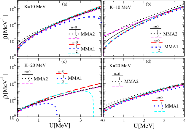
Figure 1: MMA level density $\rho$ [Eq. (42) in units of MeV^-1] as function of the excitation energy $U$ (in units of MeV) at the inverse level density parameter $K=10$ MeV (a,b), and at $20$ MeV (c,d) for the relative energy shell corrections $\mathcal{E}_{\rm sh}=1.7$ (a,c) and $0.6$ (b,d) values. The black solid ($n=0$) and dotted ($n=1$) lines are of MMA2, without [Eqs. (34)] and with [Eq. (31)] the second term, respectively. The magenta dashed line ($n=2$) [numerical, Eq. (II)] with the next leading correction term presents good convergence to the MMA2 results owing to the expansion of the Jacobian factor, $\mathcal{J}^{-1/2}$ [see Eq. (18) for the Jacobian $\mathcal{J}$], in the integrand of Eq. (II), over $1/\xi$ (see text). The heavy dashed red line ($n=0$) and blue dotted line ($n=1$), and the dashed cyan line ($n=2$) [see Eqs. (29) (MMA1) and (III.1), and (II), respectively], show the convergence to the MMA1 results due to the expansion of this Jacobian $\mathcal{J}$, over $\xi$. The particle number $A=200$ was used.

III.1 (i) Small shell effects

Using Eq. (18), one can write for small $\xi$, Eq. (20),

$$\frac{1}{\mathcal{J}^{1/2}}=\frac{1}{\sqrt{g(\lambda)\left(1+\xi\right)}}\approx\frac{1}{\sqrt{g(\lambda)}}\left(1-\frac{\overline{\xi}}{2\beta^{2}}\right)~{}.$$ (25)

Substituting this expression for the Jacobian factor, $\mathcal{J}^{-1/2}$, into Eq. (II) one obtains two terms, which are related to those of the last equation in (25). Due to the transformation of the integration variable $\beta$ to $\tau=1/\beta$ in the first term and using $\beta$ directly as the integration variable in the second term, they are reduced to the analytical inverse-Laplace form (B) for the transformation from $\tau$ to $a$ variables AS64 . Thus, one can approximately represent the level density $\rho(E,A)$ as a superposition of the two Bessel functions of the orders of 3/2 and 1/2,

$$\rho(E,A)\approx\overline{\rho}_{3/2}\left(S^{-3/2}I_{3/2}(S)-r_{1}S^{-1/2}I_{1/2}(S)\right)$$

$$\mbox{with}\quad\overline{\rho}_{3/2}=a\sqrt{\frac{2\pi}{3}}~{}.$$ (26)

Here

$$r_{1}=\frac{\overline{\xi}U^{1/2}}{4a^{3/2}}\approx\frac{\pi^{6}K^{3/2}U^{1/2}}{3\lambda^{2}A^{7/6}}~{}\mathcal{E}_{\rm sh}~{},$$ (27)

where $\overline{\xi}$ is given in Eq. (21), $K=A/a$, $a$ is the level density parameter, Eq. (13), and

$$S=2\sqrt{aU}~{}.$$ (28)

This expression is associated with an entropy in the mean field approximation because of its two clear asymptotic limits for large and small excitation energies, $U$ [both asymptotic limits in terms of the level density, $\rho(E,A)$, will be discussed below]. The relative contribution of the second term in Eq. (III.1) decreases with the shell effects, $\mathcal{E}_{\rm sh}$, inverse level density parameter, $K$, and excitation energy, $U$. In the case (i), referred to below as the MMA1 approach, up to these corrections (small $r_{1}$), one arrives approximately at expression (11) of Ref. PLB :

$$\rho(E,A)\approx\overline{\rho}_{3/2}~{}S^{-3/2}I_{3/2}(S)~{},\qquad\mbox{(i)}~{}.$$ (29)

III.2 (ii) Dominating shell effects

In this case, expanding the Jacobian factor $\mathcal{J}^{-1/2}$, see Eq. (25), over small $1/\xi$, one finds

$$\frac{1}{\mathcal{J}^{1/2}}\approx\frac{1}{\sqrt{g(\lambda)\xi}}\left(1-\frac{1}{2\xi}\right)~{},$$ (30)

where $\xi>0$, Eq. (20) (for $\delta E<0$). Substituting this approximate expression for the Jacobian factor into Eq. (II) and transforming the integration variable $\beta$ to $\tau=1/\beta$ in the integral representation for the level density $\rho(E,A)$, we obtain by using the inverse Laplace transformation (B) from $\tau$ to $a$ variable:

$$\rho(E,A)\approx\overline{\rho}_{5/2}\left(S^{-5/2}I_{5/2}(S)+r_{2}S^{-9/2}I_{9/2}(S)\right),$$ (31)

$$\mbox{with}\quad\overline{\rho}_{5/2}=4a^{2}\left(\pi/6\overline{\xi}\right)^{1/2}~{},$$ (32)

where $\overline{\xi}$ is given by Eqs. (21) and (22), and

$$r_{2}=\frac{2a^{2}}{\overline{\xi}}\approx\frac{3\lambda^{2}A^{5/3}}{2\pi^{6}K^{2}\mathcal{E}_{sh}}~{}.$$ (33)

In contrast to case (i), the relative contribution of the second term in the r.h.s. of Eq. (31) [case (ii)] has the opposite behavior in the values of parameters $\mathcal{E}_{\rm sh}$ and $K$, and is almost independent of $U$. Up to small contribution of the second term in Eq. (31), one arrives approximately at

$$\rho(E,A)\approx\overline{\rho}_{5/2}~{}S^{-5/2}I_{5/2}(S)~{},\qquad\mbox{(ii)}~{},$$ (34)

where $\overline{\rho}_{5/2}$ is given by Eq. (32). This approximation is referred to below as the MMA2 approach.

Figure 1 shows good convergence of different approximations to their main term ($n=0$) for $\rho(E,A)$. Here we accounted for the first ($n=1$) analytical and second ($n=2$) numerical corrections in the expansion of the Jacobian factor $\mathcal{J}^{-1/2}$ [see Eq. (18) for the Jacobian $\mathcal{J}$], over $1/\xi$ (MMA2) and over $\xi$ (MMA1) as functions of the excitation energy $U$. Calculations are carried out for typical values of the parameters: the inverse level density $K$, the relative energy shell corrections $\mathcal{E}_{\rm sh}$, and a large particle number $A$. The results of the analytical MMA1 approach, Eq. (III.1), and MMA2, Eq. (31), with the first correction terms, are compared with those of Eqs. (34) and (29) without first correction terms, respectively, using different values of these parameters. The contributions of these corrections to the simplest analytical expressions, Eq. (29) and (34), are smaller the smaller excitation energies $U$ for the MMA1 and the larger $U$ for the MMA2 such that a transition between the approaches, Eq. (III.1) and (31), takes place with increasing value of $U$; see Fig. 1. We also demonstrate good convergence to the leading terms ($n=0$) by taking into account numerically the next order ($n=2$ in this figure) corrections in the direct calculations of the integral representation (II). Such a convergence occurs for the MMA1 better for smaller $U$ with increasing inverse density parameter $K$ and decreasing relative energy shell correction $\mathcal{E}_{\rm sh}$. An opposite behavior takes place for the MMA2 approach. Especially, a good convergence with increasing excitation energy $U$ is seen clearly with $n=1$ and $2$ for the MMA1 in panels (a) and (c); see, e.g., panel (c) for larger values of both $K$ and $\mathcal{E}_{\rm sh}$.

Notice that for the case (ii) when the shell effects are dominating, the derivatives are relatively large, $a^{\prime\prime}(\lambda)\lambda^{2}/a\gg 1$, but at the same time the shell corrections, $\mathcal{E}_{\rm sh}$, can be small. In this case, referred to below as the MMA2b approach, we have for the coefficient $\overline{\rho}_{5/2}$

$$\overline{\rho}_{5/2}\approx 2\sqrt{2/\pi}\lambda a^{2}.$$ (35)

Here, in the calculation of $\overline{\rho}_{5/2}$ given by Eq. (32), we used the TF evaluation of the level density, $\tilde{g}\propto A/\lambda$, and its derivatives over $\lambda$ in the first equation of (21) for $\overline{\xi}$.

III.3 Disappearance of shell effects with temperature

As well known (see for instance Refs. BB03 ; SM76 ; KM79 ; MG17 ), with increasing temperatures $T$, the shell component $\delta\Omega$, Eq. (II), disappears exponentially as $\hbox{exp}(-2\pi^{2}T/D_{\rm sh})$ in the potential $\Omega$ or free energy $F$, see also Eqs. (9) and (10). This occurs at temperatures $T\approx D_{\rm sh}/\pi=2-3$ MeV ($D_{\rm sh}=\lambda/A^{1/3}=7-10$ MeV in heavy nuclei, $A\approx 100-200$). For such large temperatures with excitation energies $U$, near or larger than neutron resonances energies, one can approximate the Jacobian factor $\mathcal{J}^{-1/2}$ in Eq. (II) as

$$\mathcal{J}^{-1/2}\approx\tilde{\mathcal{J}}^{-1/2}\left(1-\delta\mathcal{J}/(2\tilde{\mathcal{J}})\right)~{},$$ (36)

where $\tilde{\mathcal{J}}\approx\tilde{g}$, and

$$\delta\mathcal{J}\approx 2\sum_{\rm PO}g_{\rm PO}x_{\rm PO}~{}\hbox{exp}\left(-x_{\rm PO}\right),$$ (37)

and $x_{\rm PO}=\pi t_{\rm PO}/\hbar\beta$, Eq. (10). With this approximation, using the transformation of the integration variable $\beta$ to $\tau=1/\beta$ in Eq. (II), one can analytically take the inverse Laplace integral [Eq. (B)] for the level density. Finally, one obtains $\rho=\tilde{\rho}+\delta\rho$, where

$$\delta\rho(E,A)=\sqrt{\frac{\pi}{2\tilde{g}^{3}}}\sum_{\rm PO}g_{\rm PO}\frac{t_{\rm PO}}{\hbar}\int\frac{{\rm d}\tau}{2\pi i\tau^{3/2}}\hbox{exp}\left(a_{\rm sh}\tau+\frac{U}{\tau}\right)$$

$$=\!\!\sqrt{\frac{\pi}{2\tilde{g}^{3}}}\sum_{\rm PO}g_{\rm PO}\frac{t_{\rm PO}}{\hbar}\left(4a~{}a_{\rm sh}\right)^{1/4}S_{\rm sh}^{-1/2}I_{1/2}\left(S_{\rm sh}\right).$$ (38)

Here, $a_{\rm sh}=\tilde{a}-\pi t_{\rm PO}/\hbar$ is the shifted level density parameter due to the shell effects, and $S_{\rm sh}=2\sqrt{a_{\rm sh}U}$ is the shifted entropy. For a major shell structure, one arrives at

$$\delta\rho(E,A)\approx\sqrt{\frac{\pi}{2\tilde{g}^{3}}}\frac{2\pi}{D_{\rm sh}}\left(4a~{}a_{\rm sh}\right)^{1/4}\delta g(\lambda)~{}S_{\rm sh}^{-1/2}I_{1/2}\left(S_{\rm sh}\right)$$

$$\approx\sqrt{\frac{\pi}{2\tilde{g}^{3}}}\left(\frac{2\pi}{D_{\rm sh}}\right)^{3}\left(4a~{}a_{\rm sh}\right)^{1/4}\delta E~{}S_{\rm sh}^{-1/2}I_{1/2}\left(S_{\rm sh}\right)$$ (39)

[see Eq. (23)], and

$$a_{\rm sh}\approx\tilde{a}-\frac{2\pi^{2}}{D_{\rm sh}}~{}.$$ (40)

Hence, the shifted inverse level-density parameter is $K=A/a~{}=~{}\tilde{K}\left(1+\Delta K/\tilde{K}\right)$, where the dimensionless shift is given by

$$\frac{\Delta K}{\tilde{K}}\approx\frac{2\pi^{2}\tilde{K}}{AD_{\rm sh}}\approx\frac{2\pi^{2}\tilde{K}}{\lambda A^{2/3}}~{}.$$ (41)

This is approximately equal to $\Delta K\approx 1-2$ MeV for $\tilde{K}=10$ MeV (see Refs. SN90 ; SN91 ; KS18 ; KS20 ) at typical parameters $\lambda=40$ MeV and $A=100-200$ ($\Delta K\approx 6-9$ MeV for $\tilde{K}=20$ MeV). We note that an important shift in the inverse level density parameter $K$ for double magic nuclei near the neutron resonances is due to a strong shell effect.

III.4 General MMA

All final results for the level density $\rho(E,A)$ discussed in the previous subsections of this section can be approximately summarized as

$$\rho\approx\rho_{\tt{MMA}}(S)=\overline{\rho}_{\nu}~{}f_{\nu}(S)~{},~{}~{}~{}f_{\nu}(S)=S^{-\nu}I_{\nu}(S)~{},$$ (42)

with corresponding expressions for the coefficient $\overline{\rho}_{\nu}$ (see above). For large entropy $S$, one finds

$$f_{\nu}(S)=\frac{\hbox{exp}(S)}{S^{\nu}\sqrt{2\pi S}}\left[1+\frac{1-4\nu^{2}}{8S}+\mbox{O}\left(\frac{1}{S^{2}}\right)\right].$$ (43)

At small entropy, $S\ll 1$, one obtains also from Eq. (42) the finite combinatorics power expansion St58 ; Er60 ; Ig72 ; Ig83

$$f_{\nu}(S)=\frac{2^{-\nu}}{\Gamma(\nu+1)}\left[1+\frac{S^{2}}{4(\nu+1)}+\mbox{O}\left(S^{4}\right)\right],$$ (44)

where $\Gamma(x)$ is the gamma function. This expansion over powers of $S^{2}\propto U$ is the same as that of the “constant temperature model” (CTM) GC65 ; ZK18 ; Ze19 , used often for the level density calculations at small excitation energies $U$, but here we have it without free parameters.

In order to clarify Eq. (43) for the MMA level density at a large entropy, one can directly obtain a more general full SPM asymptote, including the shell effects, by taking the integral over $\beta$ in Eq. (II) using the SPM (see Appendix C). We have

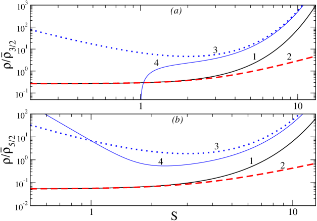
Figure 2: Level density $\rho$ [Eq. (42)], in units of $\overline{\rho}_{\nu}$, with the accurate result “1” (solid line), Eq. (29), $(a)$ for $\nu=3/2$ [MMA1 (i)], and $(b)$, Eq. (34), for $\nu=5/2$ [MMA2 (ii)], shown as functions of the entropy $S$ for different approximations: (1) $S\ll 1$ (dashed lines), Eq. (44) at the second order, and (2) $S\gg 1$ (dotted and thin solid lines),  Eq. (43); “3” is the main term of the expansion in powers of $1/S$, and “4” is the expansion over $1/S$ up to first [in $(a)$], and second [in $(b)$] order terms in square brackets of Eq. (43), respectively.

$$\rho(E,A)=\frac{\hbox{exp}(2\sqrt{aU})}{\sqrt{48}~{}U~{}\sqrt{1+\xi^{\ast}}}~{},$$ (45)

where $\xi^{\ast}$ is $\xi$ of Eq. (19) at the saddle point $\beta=\beta^{\ast}$, which is, in turn, determined by Eq. (C.2):

$$\xi^{\ast}\approx-\frac{\pi^{2}T^{2}}{6\hbar^{2}}\sum_{\rm PO}t^{2}_{\rm PO}\frac{g_{\rm PO}(\lambda)}{g(\lambda)}\approx\frac{4\pi^{6}UK\mathcal{E}_{\rm sh}}{3\lambda^{2}A^{2/3}}~{}.$$ (46)

We took the factor $\mathcal{J}^{-1/2}$, obtained from the Jacobian $\mathcal{J}$ of Eq. (18), off the integral (II) at $\beta=\beta^{\ast}=1/T$. The Jacobian ratio $\xi^{\ast}$ of $\delta\mathcal{J}/\tilde{\mathcal{J}}$ at the saddle point, $\beta=\beta^{\ast}$ ($\lambda=\lambda^{\ast}=\alpha^{\ast}T$ is the standard chemical potential of the grand-canonical ensemble), Eq. (46), is the critical quantity for these derivations. The quantity $\xi^{\ast}$ is approximately proportional to the semiclassical POT energy shell correction, $\delta E$, Eq. (23), through $\mathcal{E}_{\rm sh}$, Eq. (22), the excitation energy, $U=aT^{2}$, and to a small semiclassical parameter $A^{-1/3}$ squared for heavy nuclei (see Ref. PLB and Appendix A). For typical values of parameters, $\lambda=40$ MeV, $A\approx 200$, and $\mathcal{E}_{\rm sh}=|\delta E~{}A/E_{\rm\tt{ETF}}|\approx 2.0$ BD72 ; MSIS12 , one finds the approximate values of $\xi^{\ast}\approx 0.1-10$ for temperatures $T\approx 0.1-1$ MeV. This corresponds approximately to rather wide excitation energies $U=0.2-20$  MeV for $K=10$ MeV KS18 (and $U=0.1-10$ MeV for $K=20$  MeV). These values of $U$ overlap the interval of energies of the low energy states with that of the energies of states significantly above the neutron resonances. In line with the SCM BD72 and ETF approaches BB03 , these values are given by the realistic smooth energy $E_{\rm\tt{ETF}}$ for which the binding energy approximately equals $E_{\rm\tt{ETF}}+\delta E$ MSIS12 .

Accounting for the shell effects, Eq. (45) is more general large-excitation energy asymptote with respect to the well-known Bethe expression Be36

$$\rho(E,A)=\frac{\hbox{exp}\left(S\right)}{\sqrt{48}U}~{},$$ (47)

where such effects were neglected; see also Refs. Er60 ; GC65 ; BM67 . This expression can be alternatively obtained as the limit of Eq. (45) at large excitation energy, $U\rightarrow\infty$, up to shell effects [small $\xi^{\ast}$ of the case (i)]. This asymptotic result is the same as that of expression (29), proportional to the Bessel function $I_{\nu}$ of the order $\nu=3/2$ [the case (i)], at the main zero-order expansion in $1/S$; see Eq. (43). For large-entropy $S$ asymptote, we find also that the Bessel solution (34) with $\nu=5/2$ in the case (ii) ($\xi^{\ast}\gg 1$) at zero-order expansion in $1/S$ coincides with that of the general asymptote (45). The asymptotic expressions, Eqs. (43), (45), and, in particular, (47), for the level density are obviously divergent at $U\rightarrow 0$, in contrast to the finite MMA limit (44) for the level density; see Eq. (42) and, e.g., Eqs. (29) and (34).

Our MMA results will be compared also with the popular Fermi gas (FG) approximation to the level density $\rho(E,N,Z)$ as a function of the neutron $N$ and proton $Z$ numbers near the $\beta$ stability line, $(N-Z)^{2}/A^{2}\ll 1$ Er60 ; GC65 ; EB09 :

$$\rho(E,N,Z)=\frac{\sqrt{\pi}}{12a^{1/4}U^{5/4}}~{}\hbox{exp}\left(2\sqrt{aU}\right)~{}.$$ (48)

Notice that in all our calculations of the statistical level density, $\rho(E,A)$ [also $\rho(E,N,Z)$, Eq. (48)], we did not use a popular assumption of small spins at large excitation energy which is valid for the neutron resonances. For typical values of spin $I\hbox{\kern 1.00006pt\lower 2.58334pt\hbox{$\sim$} \kern-11.19997pt\raise 2.58334pt\hbox{$>$} \kern 1.00006pt}10$, moment of inertia $\Theta\approx\Theta_{\rm\tt{TF}}\approx 2\mu R^{2}A/5$, Eq. (A), radius $R=r_{0}A^{1/3}$, with $r_{0}=1.14$ fm, and particle number $A\hbox{\kern 1.00006pt\lower 2.58334pt\hbox{$\sim$} \kern-11.19997pt\raise 2.58334pt\hbox{$<$} \kern 1.00006pt}200$, one finds that, for large entropy, the applicability condition (B.10) is not strictly speaking valid. In these estimates, the corresponding excitation energies $U$ of LESs are essentially smaller than neutron resonance energies. However, near neutron resonances the excitation energies $U$ are large, spins are small, and Eq. (48) is well justified.

We should also emphasize that the MMA1 approximation for the level density, $\rho(E,A)$, Eq. (29), and the Fermi gas approximation, Eq. (47) can be also applied for large excitation energies $U$, with respect to the collective rotational excitations, if one can neglect shell effects, $\xi^{\ast}\ll 1$. Thus, with increasing temperature $T\hbox{\kern 1.00006pt\lower 2.58334pt\hbox{$\sim$} \kern-11.19997pt\raise 2.58334pt\hbox{$>$} \kern 1.00006pt}1$ MeV (if it exists), or excitation energy $U$, where the shell effects are yet significant, one first obtains the asymptotical expression (45) at $\xi^{\ast}\gg 1$, i.e., the asymptote of Eq. (34). Then, with further increasing temperature to about 2-3 MeV with the disappearance of shell effects (section III.3), one gets the transition to the Bethe formula, i.e., the large entropy asymptote (47) of Eq. (29).

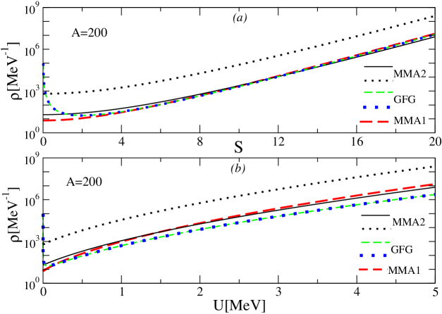
Figure 3: MMA level density $\rho$ [Eq. (42)] in units of MeV^-1 as function of the entropy $S$ (a), and excitation energy $U$, in units of MeV (b). The black solid and dotted lines are the MMA2 approach for $\mathcal{E}_{\rm sh}=2.0$ and $0.002$, Eq. (34), respectively. Green dashed and blue dotted lines are the general Fermi gas (GFG) approach, Eq. (45), for the same values of $\mathcal{E}_{\rm sh}$, respectively. The red dashed line is the MMA1, Eq. (29); in (b) $K=10$ MeV, of the order of the ETF value of Ref. KS18 .

In Fig. 2 we show the level density dependence $\rho(S)$, Eq. (42), for $\nu=3/2$ in $(a)$ and $\nu=5/2$ in $(b)$, on the entropy variable $S$ with the corresponding asymptote. In this figure, small [$S\ll 1$, Eq. (44)] and large [$S\gg 1$, Eq. (43)] entropy $S$ behaviors are presented. For small $S\ll 1$ expansion we take into account the quadratic approximation “2”, where $S^{2}\propto U$, that is the same as in the linear expansion within the CTM GC65 ; ZK18 . For large $S\gg 1$ we neglected the corrections of the inverse power entropy expansion of the preexponent factor in square brackets of Eq.  (43), lines “3”, and took into account the corrections of the first [$\nu=3/2$, $(a)$] and up to second [$\nu=5/2$, $(b)$] order in $1/S$ (thin solid lines “4”) to show their slow convergence to the accurate MMA result “1” (42). It is interesting to find almost a constant shift of the results of the simplest, $\rho\propto\hbox{exp}(S)/S^{\nu+1/2}$, SPM asymptotic approximation at large $S$ (dotted lines “3”) with respect to the accurate MMA results of Eq. (42) (solid lines “1”). This may clarify one of the phenomenological models, e.g., the back-shifted Fermi-gas (BSFG) model for the level density DS73 ; So90 ; EB09 .

Figure 3 shows the shell effects in the main approximations derived in this section, Eqs.(29), (34), and (45), taking two essentially different values of finite $\mathcal{E}_{\rm sh}=2.0$ and much smaller $0.002$, between which one can find basically those given by Ref. MSIS12 . For convenience, we show these results as functions of the entropy $S$ in panel (a), and the excitation energy $U$ in panel (b), taking the value of the averaged inverse density parameter $K$ found in Ref. KS18 ; see also Ref. KS20 . As expected, the shell effect is very strong for the MMA2 approach, as can be seen from the difference between solid and dotted black lines depending on the second derivatives of strong oscillating functions of $\lambda$, $a^{\prime\prime}(\lambda)\approx\delta a^{\prime\prime}\propto\delta g^{\prime\prime}(\lambda)$ [see Appendix A around Eq. (A.17) and Sec. III below Eq. (23)]. This is not the case for the full SPM asymptotic GFG, Eq. (45), for which this effect is very small. As seen from this figure, the MMA1, Eq. (29), independently of $\mathcal{E}_{\rm sh}$, converges rapidly to the GFG with increasing excitation energy $U$ as well as to the Bethe formula (47). They all coincide at small values of $U$, about 0.5 MeV, particularly for $\mathcal{E}_{\rm sh}=0.002$. The Bethe approach is very close everywhere to the GFG line at $\mathcal{E}_{\rm sh}=0.002$ and therefore, it is not shown in this figure. Notice also that MMA2 at this small $\mathcal{E}_{\rm sh}$ is also close to the MMA1 everywhere. Again, one can see that the MMA1 and MMA2 have no divergence at zero excitation energy limit, $U\rightarrow 0$, while the full SPM asymptotic GFG, Eq. (45), and, in particular, the Bethe approach, Eq. (47), both diverge at $U\rightarrow 0$.

III.5 The spin-dependent level density

Assuming that there are no external forces acting on an axially symmetrical nuclear system, the total angular momentum $I$ and its projection $M$ on a space-fixed axis are conserved, and states with a given energy $E$ and spin $I$ are $2I+1$ degenerated. As shown in Appendix B, for the “parallel” rotation around the symmetry axis $Oz$, i.e., an alignment of the individual angular momenta of the particle along $Oz$ (see Ref. KM79 for the spherical case), in contrast to the “perpendicular-to-axis $Oz$” collective rotation (see, e.g., Ref. GM21 ), one can derive the level density $\rho(E,A,M)$ within the MMA approach in the same analytical form as for the $\rho(E,A)$, Eq. (42):

$$\rho_{\rm\tt{MMA}}(E,A,M)\approx\overline{\rho}_{\nu}f_{\nu}(S)~{},\qquad\mbox{with}\qquad\nu=2,3~{},$$ (49)

where

$$\overline{\rho}_{2}=\hbar~{}\left(\frac{2a^{3}}{3\Theta}\right)^{1/2},\quad\nu=2~{}~{}~{}\mbox{(}i)~{},$$ (50)

and

$$\overline{\rho}_{3}=\hbar\lambda~{}\left(\frac{8a^{5}}{\pi^{2}\Theta}\right)^{1/2},\quad\nu=3~{}~{}~{}(ii)~{}.$$ (51)

In Eq. (49), the argument of the Bessel-like function, $f_{\nu}(S)\propto I_{\nu}(S)$, Eq. (42), is the entropy $S(E,A,M)$, Eq. (28), with the $M$-dependent excitation energy $U$. Indeed, in the adiabatic mean-field approximation, the level density parameter $a$ in Eq. (28) is given by Eq. (14). For the intrinsic excitation energy $U$ in Eq. (28), one finds

$$U=E-E_{0}-\frac{1}{2}\Theta~{}\omega^{2}~{},~{}~{}~{}~{}\omega=\frac{\hbar M}{\Theta}~{},$$ (52)

where, $E_{0}=\tilde{E}+\delta E$, is the same intrinsic (nonrotating) shell-structure energy as in Eq. (12). With the help of the conservation equation (B.3) for the saddle point, $\kappa^{\ast}=\hbar\omega\beta$, we eliminated the rotation frequency $\omega$, obtaining the second equation in Eq. (52); see Appendix B. For the moment of inertia (MI) $\Theta$ one has a similar SCM decomposition:

$$\Theta=\tilde{\Theta}+\delta\Theta~{},$$ (53)

where $\tilde{\Theta}$ is the (E)TF MI component which can be approximated largely by the TF expression, Eq. (A), and $\delta\Theta$ is the MI shell correction which can be presented finally for the spherically symmetric mean field by Eq. (B.5). As mentioned above, Eqs. (49)-(53) are valid for the “parallel” rotation (an alignment of nucleons’ angular momenta along the symmetry axis $Oz$); see Appendix B for the specific derivations by assuming a spherical symmetry of the potential. In these derivations we used Eq. (52) for the excitation energy $U$, Eq. (A) for the partition function and Eqs. (B.9) and (A.8) for the potential $\Omega(\beta,\lambda,\omega)$. In the evaluations of the Jacobian, $\mathcal{J}$, one can neglect shell corrections, in contrast to the evaluations of the entropy $S$ in the function $f_{\nu}(S)$. In the derivations of Eqs. (50) for $\overline{\rho}_{2}$ and (51) for $\overline{\rho}_{3}$, we obtained the Jacobian components, $\tilde{\mathcal{J}}$ for the case (i) and $\delta\mathcal{J}$ for the case (ii), both under the assumption of an axially symmetric mean field (see Appendix B). For the Jacobian calculations, one can finally use the (E)TF approximation in the case (i), $\Theta\approx\tilde{\Theta}$. The Jacobian $\mathcal{J}$ in the case (ii) can be approximated by Eq.  (B.14). As a result, one may accurately use the (E)TF approximation $\Theta\approx\tilde{\Theta}$ in Eqs. (50) and (51) for the coefficients $\overline{\rho}_{2}$ and $\overline{\rho}_{3}$.

Note that there is no divergence of the level density $\rho(E,A,M)$ [Eq. (49)] in the limit $U\rightarrow 0$, Eq. (44), in contrast to the standard results of the full SPM within the Fermi gas model. The latter is associated with the leading term in expansion (43) of the Bessel-like function $f_{\nu}(S)$.

Equation (49), with $M=\mathcal{K}$, if it exists, can be used for the calculations of the level density $\rho(E,A,\mathcal{K})$, where $\mathcal{K}$ is the specific projection of the total angular momentum ${\bf I}$ on the symmetry axis of the axially symmetric potential MK79 (K in notations of Ref. BM75 ). We note that it is common to use in application Be36 ; Er60 ; BM67 the level density dependence on the spin $I$, $\rho(E,A,I)$. We will consider here only the academic axially symmetric potential case which can be realized practically for the spherical or axial symmetry of a mean nuclear field for the “parallel” rotation mentioned above. Using Eq. (49), under the same assumption of a closed rotating system and, therefore, with conservation of the integrals of motion, the spin $I$ and its projection $M$ on the space-fixed axis, one can calculate the corresponding spin-dependent level density $\rho(E,A,I)$ for a given energy $E$, particle number $A$, and total angular momentum $I$ by employing the Bethe formula Be36 ; BM67 ; Ig83 ; So90 ,

$$\rho(E,A,I) = \rho(E,A,M=I)-\rho(E,A,M=I+1)$$ (54)

$$\approx -\left(\frac{\partial\rho(E,A,M)}{\partial M}\right)_{M=I+1/2}~{}.$$

For this level density, $\rho(E,A,I)$, one obtains from Eqs. (49) and (52),

$$\rho_{\rm\tt{MMA}}(E,A,I)\approx\frac{a\overline{\rho}_{\nu}\hbar^{2}(2I+1)}{\Theta}f_{\nu+1}(S)~{},$$ (55)

where $S$ is given by Eq. (28) with the excitation energy (52), and $\nu$ equals 2 and 3, in correspondence with Eq. (49). The multiplier $2I+1$ in Eq. (55) appears because of the substitution $M=I+1/2$ into the derivative in Eq. (54). In order to obtain the approximate MMA total level density $\rho(E,A)$ from the spin-dependent level density $\rho(E,A,I)$ we can multiply Eq. (55) by the spin degeneracy factor $2I+1$ and integrate (sum) over all spins $I$.

Using the expansion of the Bessel functions in Eq. (55) over the argument $S$ for $S\ll 1$ [Eq. (44)] one finds the finite combinatorics expression. For large $S$ [large excitation energy, $aU\gg 1$, Eq. (43)], one obtains from Eq. (55) the asymptotic Fermi gas expansion. Again, the main term in the expansion for large $S$, Eq. (43), coincides with the full SPM limit to the inverse Laplace integrations in Eq. (B). For small angular momentum $I$ and large excitation energy $U_{0}=E-E_{0}$, so that

$$\frac{E_{\rm rot}}{U_{0}}\approx\frac{I(I+1)\hbar^{2}}{2\Theta~{}U_{0}}\ll 1~{},$$ (56)

one finds the standard separation of the level density, $\rho_{\rm\tt{MMA}}(E,A,I)$, into the product of the dimensionless spin-dependent Gaussian multiplier, $\mathcal{R}(I)$, and another spin-independent factor. Finally, for the case (i) ($\nu=2$), one finds

$$\rho_{\rm\tt{MMA}}(E,A,I)\approx\frac{\overline{\rho}_{2}~{}\mathcal{R}(I)~{}\hbox{exp}\left(2\sqrt{aU_{0}}\right)}{16\sqrt{\pi}~{}(aU_{0})^{5/4}}\quad(i)~{}.$$ (57)

The spin-dependent factor $\mathcal{R}(I)$ is given by

$$\mathcal{R}(I)=\frac{2I+1}{q^{2}}\hbox{exp}\left(-\frac{I(I+1)}{2q^{2}}\right)~{},$$ (58)

where $q^{2}=\Theta\sqrt{U_{0}/a}/\hbar^{2}$ is the dimensionless spin dispersion. This dispersion $q$ at the saddle point, $\beta^{\ast}=1/T=\sqrt{a/U_{0}}$, is the standard spin dispersion $\Theta T/\hbar^{2}$; see Refs. Be36 ; Er60 . Similarly, for the $\nu=3$ (ii) case one obtains

$$\rho_{\rm\tt{MMA}}(E,A,I)\approx\frac{\overline{\rho}_{3}~{}\mathcal{R}(I)~{}\hbox{exp}\left(2\sqrt{aU_{0}}\right)}{32\sqrt{\pi}~{}(aU_{0})^{7/4}}\quad(ii)~{}.$$ (59)

Note that the power dependence of the preexponent factor of the level density $\rho(E,A,I)$ on the excitation energy, $U_{0}=E-E_{0}$, differs from that of $\rho(E,A,M)$; see Eqs. (49) and (43). The exponential dependence, $\rho\propto\hbox{exp}(2\sqrt{a(E-E_{0})})$, for large excitation energy $E-E_{0}$ is the same for $\nu=2$ (i) and $3$ (ii), but the pre-exponent factor is different; cf. Eqs. (57) and (59). A small angular momentum $I$ means that the condition of Eq. (56) was applied. Equations (57) and (59) with Eq. (58), are valid for excited states within approximately the condition $1/\tilde{g}\ll U\ll\lambda$; see Eq. (24). For relatively small spins [Eq. (56)] we have the so-called small-spins Fermi-gas model (see, e.g., Refs. Be36 ; Er60 ; GC65 ; BM67 ; Ig83 ; So90 ; KS20 ).

General derivations of equations applicable for axially symmetric systems (a “parallel” rotation) in this section are specified in Appendix B by using the spherical potential to present explicitly the expressions for the shell correction components of several POT quantities. However, the results for the spin-dependent level density, $~{}\rho(E,A,I)$ in this section, Eqs. (55)-(59), cannot be immediately applied for comparison with the available experimental data on rotational bands in the collective rotation of a deformed nucleus. They are presented within the unified rotation model BM75 in terms of the spin $I$ and its projection $\mathcal{K}$ to the internal symmetry axis for the deformed nuclei. We are going to use the ideas of Refs. Bj74 ; BM75 ; Gr13 ; Gr19 ; Ju98 (see also Refs. Ig83 ; So90 ) concerning another definition of the spin-dependent level density $\rho(E,A,I)$ in terms of the intrinsic level density and collective rotation (and vibration) enhancement in a forthcoming work. The level density $\rho(E,A,\mathcal{K})$, e.g., Eq. (49) at $M=\mathcal{K}$, depending on the spin projection $\mathcal{K}$ on the symmetry axis of an axially-symmetric deformed nucleus, can be helpful in this work.

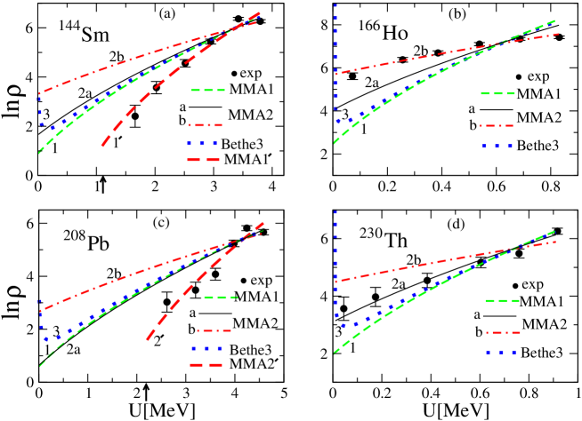
Figure 4: Level density, $\mbox{ln}\rho(E,A)$, is obtained for low energy states in ¹⁴⁴Sm (a), ¹⁶⁶Ho (b), ²⁰⁸Pb (c) and ²³⁰Th (d) within different approximations: The MMA dashed green line “1”, Eq. (29); the MMA solid black line “2a”, Eq. (34), at the relative realistic shell correction $\mathcal{E}_{\rm sh}$ MSIS12 ; the MMA dash-dotted red “2b”, Eq. (34) at an extremely small $\mathcal{E}_{\rm sh}$, Eq. (34) with (35); and the Fermi gas Bethe3 rare blue dotted line, Eq. (47). The realistic values of $\mathcal{E}_{\rm sh}$= 0.37 (a), 0.50 (b), 1.77 (c), and 0.55 (d) for MMA2 are taken from Ref. MSIS12 (the chemical potential $\lambda=40$ MeV, independent of particle numbers). Heavy dashed red lines test shifts of the excitation energies $U$ for MMA1 and MMA2a by +$1.1$ and $+2.2$ MeV in ¹⁴⁴Sm and ²⁰⁸Pb, respectively, which are due, presumably, to the pairing condensation energy shown by arrows in the panels $(a)$ and $(c)$, as explained in the text and Table 1. Experimental dots (with error bars, $\Delta\rho_{i}/\rho_{i}=1/\sqrt{N_{i}}$) are obtained directly from the excitation states (with spins and their degeneracies) spectrum ENSDFdatabase in shown nuclei (Table 1) by using the sample method where the sample lengths $U_{s}=0.45(a),0.15(b),0.34(c)$, and $0.17(d)$ MeV are found on the plateau condition over the inverse level density parameter $K$.

IV Discussion of the results

In Fig. 4 and Table 1 we present results of theoretical calculations of the statistical level density $\rho(E,A)$ (in logarithms) within the MMA, Eq. (42), and Bethe, Eq. (47), approaches as functions of the excitation energy $U$ and compared with experimental data. The results of the popular FG approach, Eq. (48), and our GFG, Eq. (45), are very close to those of the Bethe approximation and, therefore, they are presented only in Table 1. All of the presented results are calculated by using the values of the inverse level density parameter $K$ obtained from their least mean-square fits (LMSF) to experimental data for several nuclei. The data shown by dots with error bars in Fig. 4 are obtained for the statistical level density $\rho(E,A)$ from the experimental data for the excitation energies $U$ and spins $I$ of the states spectra ENSDFdatabase by using the sample method: $\rho_{i}^{\rm exp}=N_{i}/U_{s}$, where $N_{i}$ is the number of states in the $i$th sample, $i=1,2,...,N_{\rm tot}$; see, e.g., Refs. So90 ; LLv5 . The dots are plotted at mean positions $U_{i}$ of the excitation energies for each $i$th sample. Convergence of the sample method over the equivalent sample-length parameter $U_{s}$ of the statistical averaging was studied under statistical plateau conditions, for all plots in Fig. 4. The sample lengths $U_{s}$ play a role which is similar to that of averaging parameters in the Strutinsky smoothing procedure for the SCM calculations of the averaged s.p. level density St67 ; BD72 . This plateau means almost constant value of the physical parameter $K$ within large enough energy intervals $U_{s}$. A sufficiently good plateau was obtained in a wide range around the values near $U_{s}$ for nuclei presented in Fig. 4 and Table 1 ENSDFdatabase ; HJ16 . Some values of $U_{s}$ are given in the caption of Fig. 4. Therefore, the results of Table 1, calculated at the same values of the found plateau, do not depend, with the statistical accuracy, on the averaging parameter $U_{s}$ within the plateau. This is similar to the results that the energy and density shell corrections are independent of the smoothing parameters in the SCM. The statistical condition, $N_{i}\gg 1$ at $N_{\rm tot}\gg 1$, determines the accuracy of our calculations. Microscopic details are neglected under these conditions, but one obtains more simple, general, and analytical results, in contrast to a micro-canonical approach. As in the SCM, in our calculations by the sample method with good plateau values for the sample lengths $U_{s}$ (see the caption of the Fig. 4), one obtains a sufficiently smooth statistical level density as a function of the excitation energy $U$. We require such a smooth function because the statistical fluctuations are neglected in our theoretical derivations.

Nuclei	$\langle\Delta\rho_{i}/\rho_{i}\rangle$	$\mathcal{E}_{\rm{sh}}$	Version	K [MeV]	$\sigma$		Version	K [MeV]	$\sigma$
Sm-144	0.18	0.37	MMA2b	40.3	5.1		MMA1∗	22.7 (16.7∗)	3.6 (3.3∗)
			GFG	21.8	3.8		MMA2a	22.1	3.9
			Bethe	23.2	3.7		FG	19.7	3.6
Sm-148	0.17	0.12	MMA2b	32.5	5.2		MMA1	16.8	1.5
			GFG	16.9	1.7		MMA2a	19.3	3.0
			Bethe	17.2	1.7		FG	14.6	1.6
Ho-166	0.09	0.50	MMA2b	17.5	1.6		MMA1	5.4	12.3
			GFG	5.5	11.1		MMA2a	7.1	7.0
			Bethe	5.6	11.2		FG	4.7	11.5
Pb-208	0.20	1.77	MMA2b	70.1	3.8		MMA1	43.9	3.1
			GFG	36.5	3.1		MMA2a∗	34.9 (21.9∗)	3.0 (2.4∗)
			Bethe	45.1	3.2		FG	38.2	3.1
Th-230	0.24	0.55	MMA2b	36.8	2.6		MMA1	12.3	2.1
			GFG	12.7	1.3		MMA2a	14.9	0.9
			Bethe	12.9	1.3		FG	10.8	1.3

Table 1: The maximal mean errors (second column) in the statistical distribution of the states over the samples, $\langle\Delta\rho_{i}/\rho_{i}\rangle=\langle 1/\sqrt{N_{i}}\rangle$, in nuclei (first column) from Ref. ENSDFdatabase ; the relative energy shell corrections $\mathcal{E}_{\rm sh}$, Eq. (22) (third column, from Ref. MSIS12 ); the inverse level density parameter $K$ (fifth and eighth columns), found by the LMSF with the precision of the standard expression for $\sigma$, Eq. (60), (sixth and ninth columns) by using the sample method and experimental data from Ref. ENSDFdatabase , are shown for the version of the approximation in the fourth and seventh columns at the relative shell corrections $\mathcal{E}_{\rm sh}$ of the third column. The MMA1 and MMA2b (with the same notations for different MMA as in Fig. 4) are MMA approaches (29) ($\nu=3/2$) and (34) ($\nu=5/2$ at extremely small $\mathcal{E}_{\rm sh}$); GFG is the general full Fermi gas asymptote (45). The MMA2a is a more general MMA, Eq. (34), at different relative shell corrections $\mathcal{E}_{\rm sh}$ MSIS12 . The asterisks denote the MMA1 and MMA2a approaches which are shifted along the excitation energy $U$ axis by the assumed pairing condensation energy $E_{\rm cond}\approx 1.1$ and $2.2$ MeV, $U\rightarrow U-E_{\rm cond}$, for ¹⁴⁴Sm and ²⁰⁸Pb as shown in parentheses, respectively (see Sec. IV). Bethe [Eq. (47)] and FG [Eq. (48)] approaches are the same as in Refs. Be36 ; Er60 ; GC65 .

The relative quantity $\sigma$ of the standard LMSF (see Table 1), which determines the applicability of the theoretical approximations, $\rho(U_{i})$ (Sec. III) for the description of the experimental data ENSDFdatabase $\rho_{i}^{\rm exp}$, is given by

$$\sigma^{2}=\frac{\chi^{2}}{N_{\rm tot}-1}~{},\quad\chi^{2}=\sum_{i=1}^{N_{\rm tot}}\frac{(y(U_{i})-y^{\rm exp}_{i})^{2}}{(\Delta y_{i})^{2}}~{},$$ (60)

where $y=\ln\rho$ and $\Delta y_{i}\approx 1/\sqrt{N_{i}}$. For the theoretical approaches one has the conditions of the applicability assumed in their derivations. We consider the commonly accepted Fermi gas asymptote Be36 ; Er60 ; BM67 ; LLv5 ; Ig83 ; So90 for large excitation energies $U$; see the Bethe [Eq. (47)] and FG [Eq. (48)] approaches, cf. with Eq. (43) and our GFG (with shell effects) expression (45). In a forthcoming work we will use the asymptote of Eqs. (43) and (45), and the sample method for evaluations of the statistical accuracy of the experimental data at relatively large excitation energies (near and higher than neutron resonances). It is especially helpful in the case of low-resolution dense states at sufficiently large excitation energies. The examination using the value of $\sigma$ obtained by the LMSF is an additional procedure for examining these theoretical conditions, using the available experimental data. Notice also that application of the sample method in determining the experimental statistically averaged level density from the nuclear spectra in terms of $\sigma^{2}$ differs essentially from the methods employed in previous works (see, e.g., Ref. EB09 ) by using the statistical averaging of the nuclear level density and accounting for the spin degeneracies of the excited states. We do not use empiric free parameters in all of our calculations, in particular, for the FG results shown in Table 1. The commonly accepted nonlinear FG asymptote (43) could be a critical (necessary but, of course, not sufficient) theoretical guide which, with a given statistical accuracy, is helpful for understanding spectrum completeness of the experimental data at large excitation energies where the spectrum is very dense.

Figure 4 shows the two opposite situations concerning the state distributions as functions of the excitation energy $U$. We show results for the spherical magic ¹⁴⁴Sm (a) and double magic ²⁰⁸Pb (c) nuclei with maximal (in absolute value but negative) shell correction energies, in terms of the positive, $~{}\mathcal{E}_{\rm sh}$; see Table 1 and Ref. MSIS12 . In these nuclei, there are almost no states with extremely low excitation energies in the range of $U\hbox{\kern 1.00006pt\lower 2.58334pt\hbox{$\sim$} \kern-11.19997pt\raise 2.58334pt\hbox{$<$} \kern 1.00006pt}1-2$ MeV ENSDFdatabase . In Table 1, we present also results for the deformed nucleus ¹⁴⁸Sm where only a few levels exist in such a range which yields entropies $S\hbox{\kern 1.00006pt\lower 2.58334pt\hbox{$\sim$} \kern-11.19997pt\raise 2.58334pt\hbox{$<$} \kern 1.00006pt}1$. For the significantly deformed nucleus ¹⁶⁶Ho, with intermediate values of $\mathcal{E}_{\rm sh}$ between minimum and maximum [Fig. 4(b)], one finds the opposite situation when there are many such LESs. An intermediate number of LESs is observed, e.g., in another deformed nucleus, ²³⁰Th [Fig. 4(d)], which has a complicated strong shell structure including subshell effects MSIS12 . Thus, we also present the results for two deformed nuclei, ¹⁶⁶Ho and ²³⁰Th, from both sides of the desired heavy particle-number interval $A\approx 140-240$.

In Fig. 4, the results of the MMA approaches (1 and 2) are compared with those of the well-known “Bethe3” Be36 [Eq. (47)] asymptote; see also Table 1 for these and a few other asymptotical approaches, the FG [Eq. (48)] and, with a focus on shell effects, GFG [Eq. (45)]. Results for the MMA2a, the MMA2 [Eq. (34)] at the dominating shell effect case (ii) [$\xi^{\ast}\gg 1$, Eq. (46), in the saddle point $\beta=\beta^{\ast}$ for large excitation energies $U$], and for those with realistic relative shell correction $\mathcal{E}_{\rm sh}$ MSIS12 , are shown versus the results of a small shell effects approach MMA1 (i), Eq. (29) ($\xi^{\ast}\ll 1$ at $\beta=\beta^{\ast}$). For a very small value of $\mathcal{E}_{\rm sh}$, but still within the values of the case (ii), Eq. (34) with (35) (in particular, large $\xi^{\ast}$), we have the approach named MMA2b. Results for the MMA2b approach are also shown in Fig. 4. Results of calculations within the full SPM GFG asymptotical approach, Eq. (45), and within the popular FG approximation, Eq. (48), which are in good agreement with the standard Bethe3 approximation, are only presented in Table 1. For finite realistic values of $\mathcal{E}_{\rm sh}$, the results of the MMA2a approach are closer to those of the MMA1 approach. Therefore, since the MMA2b approach, Eqs. (34) with (35), is the limit of the MMA2 one at a very small $\mathcal{E}_{\rm sh}$ within the case (ii), we conclude that the MMA2 approach is a more general shell-structure MMA formulation of the statistical level-density problem.

In all panels of Fig. 4, one can see the divergence of the level densities of the Bethe formula [also, the FG, Eq. (48), and the GFG, Eqs. (45) and (43)], near the zero excitation energy, $U\rightarrow 0$. This is, obviously, in contrast to any MMAs, combinatorics expression (44) in the limit of zero excitation energy; see Eqs. (42), (29), and (34). The MMA1 results are close to the Bethe, FG and GFG approaches everywhere, for all presented nuclei. The reason is that their differences are essential only for extremely small excitation energies $U$ where MMA1 is finite while other (Bethe, FG and GFG) approaches are divergent. However, there are almost no excited states in the range of their differences in the nuclei under consideration.

The results of the MMA2b approach [the same as MMA2 approach, Eq. (34) but with Eq. (35) for the coefficient $\overline{\rho}_{5/2}$, at relatively very small shell correction, $\mathcal{E}_{\rm sh}$] within the case (ii), for ¹⁶⁶Ho [see Fig. 4(b)] with $\sigma$ of the order of one are in significantly better agreement with experimental data as compared to the results of all other approaches (for the same nucleus). The MMA1 [Eq. (29)], Bethe [Eq. (47)], FG [Eq. (48)], and full SPM GFG [Eq. (45)] approaches are characterized by values of $\sigma\gg 1$, which are largely of the order of 10 (see Table 1). In contrast to the ¹⁶⁶Ho excitation energy spectrum with many very LESs below about 1 MeV, for ¹⁴⁴Sm (a) and ²⁰⁸Pb (c) one finds no such states. For the MMA2b [MMA2 for very small $\mathcal{E}_{\rm sh}$, but within the (ii)] approach we have larger values of $\sigma$, $\sigma\gg 1$ for ^144,148Sm and little larger for ²⁰⁸Pb, versus those of other approximations. In particular, for MMA1 (i), and the other asymptotic approaches of Bethe, FG, and GFG, one finds almost the same $\sigma$ of the order of one, that is in better agreement with data ENSDFdatabase ; HJ16 . We obtain basically the same for MMA2a (ii) with realistic values of $\mathcal{E}_{\rm sh}$. Notice that for ^144,148Sm and ²⁰⁸Pb nuclei, the MMA2a [Eq. (34)] at realistic $\mathcal{E}_{\rm sh}$ is close to the MMA1 (i), Bethe, FG, and GFG approaches. The MMA1 and MMA2a (at realistic values of $\mathcal{E}_{\rm sh}$) as well as Bethe, FG and GFG approaches are obviously in much better agreement with experimental data ENSDFdatabase for ¹⁴⁴Sm (or ¹⁴⁸Sm) and ²⁰⁸Pb [Fig.  4(a) and (c)], for which one has the opposite situation: very small states number in the LES range.

We note that the results of the MMA1 and MMA2a with shifted excitation energies $U\rightarrow U_{\rm eff}=U-E_{\rm cond}>0$ by constant condensation energies $E_{\rm cond}\approx 1.1$ and $2.2$ MeV, shown by arrows in Fig. 4 for ¹⁴⁴Sm and ²⁰⁸Pb, respectively, may indicate the pairing phase transition effect because of disappearance of the pairing correlations Ig83 ; So90 ; SC19 . With increasing $U$, one can see a sharp jump in the level density for the double magic ²⁰⁸Pb nucleus within the shown spectrum range. In ¹⁴⁴Sm, one finds such a phase transition a little above the presented range of the excitation energies. This effect could be related to the pairing phase transition near the critical temperature $T_{\rm cr}=0.47$ MeV in ²⁰⁸Pb ($0.57$ MeV in ¹⁴⁴Sm), i.e. at the critical effective excitation energy, $U_{\rm eff}=U-E_{\rm cond}\approx 3.3$ MeV ($4.1$ MeV in ¹⁴⁴Sm), resulting in a level density jump. These simple estimates show a qualitative agreement, by order of magnitude, with the condensation energy, $E_{\rm cond}\approx 1$ MeV. This procedure is a self-consistent calculation. Starting from a value of the condensation energy, $E_{\rm cond}$, one can obtain the inverse level density parameter $K$. Then, one evaluates a new $E_{\rm cond}$ and reiterates till convergence in the values of $K$ and $E_{\rm cond}$ is achieved, at least in order of the magnitudes. This can be realized for the MMA1 for ¹⁴⁴Sm and MMA2a for ²⁰⁸Pb; see Table 1 and Fig. 4(a) and (c). The phase transition jump is well seen in the plot (c) but is not seen in plot (a) being above the excitation energy range, at both the effective excitation energies $U_{\rm eff}$ mentioned above.

One of the reasons for the exclusive properties of ¹⁶⁶Ho [Fig. 4(b)] as compared to both ¹⁴⁴Sm (a) and ²⁰⁸Pb (c) might be assumed to be the nature of the excitation energy in these nuclei. Our MMA (i) or (ii) approaches could clarify the excitation nature [see Sec. III.5 and Appendix B for the rotational contribution which can be included in $E_{0}$ of Eq. (12) as done in Eq. (B.6)]. Since the results of the MMA2b (ii) approach are in much better agreement with experimental data than those of the MMA1 (i) approach for ¹⁶⁶Ho, one could presumably conclude that for ¹⁶⁶Ho one finds more clear thermal excitations, $U\gg E_{\rm rot}$, Eq. (24), for LESs. For ¹⁴⁴Sm and ²⁰⁸Pb one observes more regular (large spins owing to the alignment) excitation contributions for dominating rotational energy $E_{\rm rot}$, Eq. (B.10); see Ref. KM79 . The latter effect is much less pronounced in ²⁰⁸Pb than in ¹⁴⁴Sm, but all the inverse level density parameters $K$ are significant for states below neutron resonances; see Table 1. However, taking into account the pairing effects, even qualitatively, the thermal contribution (ii) is also important for ²⁰⁸Pb while the regular nonthermal motions might be dominating in ¹⁴⁴Sm. In any case, the shell effects are important, especially for the (ii) case which does not even exist without taking them into account.

For ²³⁰Th [Fig.  4(d)], one has the experimental LESs data in the middle of two limiting cases MMA1 (i) and MMA2b (ii). This agrees also with an intermediate number of very LESs in this nucleus. As shown in Fig. 4(d) and Table 1, the MMA2a approach at realistic values of $\mathcal{E}_{\rm sh}$ is in good agreement with the data. The shell structure is, of course, not so strong in ²³⁰Th as compared to that of the double magic nucleus, ²⁰⁸Pb, but it is of the same order as in other presented nuclei. Also notice that, in contrast to the spherical nuclei in Figs. 4 (a) and (c), the nuclei ¹⁶⁶Ho (b) and ²³⁰Th (d) are significantly deformed, which is also important, in particular, because of their large angular momenta of the LES excitation spectrum states.

We do not use free empiric parameters of the BSFG, spin cutoff FG, and empiric CTM approaches EB09 . As an advantage, one has only the parameter $K$ with the physical meaning of the inverse level density parameter. The variations in $K$ are related, e.g., to those of the mean field parameters through Eq. (28). All the densities $\rho(E,A)$ compared in Fig. 4 and Table 1 do not depend on the cutoff spin factor and moment of inertia because of summation (integrations) over all spins (however, with accounting for the degeneracy $2I+1$ factor).

In line with the results of Ref. ZS16 , the obtained values of $K$ for the MMA2 approach can be essentially different from the MMA1 ones and those (e.g., FG) found, mainly, for the neutron resonances (NRs). However, the level densities with the excitation energy shifted by constant condensation energies, due to pairing, for ²⁰⁸Pb (c) and ¹⁴⁴Sm (a) in Fig. 4, notably improve the comparison with data ENSDFdatabase . These densities correspond to inverse level-density parameters $K$, smaller even than those obtained in the FG approach which agreed with NR data. We note that for the MMA1 approach one finds values of $K$ which are of the same order as those of the Bethe, FG and GFG approaches. These values of $K$ are mostly close to the NR values in order of magnitude. For the FG approach, Eq. (48), in accordance with its nondirect derivation through the spin-dependent level density $\rho(E,A,I)$, Eq. (57) (Sec. III.5), it is obviously because the neutron resonances occur at large excitation energies $U$ and small spins; see Eqs. (24) and (56). Large deformations, neutron-proton asymmetry, spin dependence for deformed nuclei, and pairing correlations Er60 ; Ig83 ; So90 ; AB00 ; AB03 ; ZK18 ; Ze19 in rare earth and actinide nuclei should be also taken into account to improve the comparison with experimental data.

V Conclusions

We derived the statistical level density $\rho(S)$ as function of the entropy $S$ within the micro-macroscopic approximation (MMA) using the mixed micro- and grand-canonical ensembles beyond the standard saddle point method of the Fermi gas model. The obtained level density can be applied for small and relatively large entropies $S$ or excitation energies $U$ of a nucleus. For a large entropy (excitation energy), one obtains the exponential asymptote of the standard SPM Fermi gas model, but with significant powers of $1/S$ corrections. For small $S$ one finds the usual finite combinatorics expansion in powers of $S^{2}$. Functionally, the MMA at linear approximation in $S^{2}\propto U$ expansion, at small excitation energies $U$, coincides with the empiric constant “temperature” model except it is obtained without using free fitting parameters. Thus, MMA unifies the commonly accepted Fermi gas approximation with the empiric CTM for large and small entropies $S$, respectively, in line with the suggestions in Refs. GC65 ; ZK18 . The MMA clearly manifests an advantage over the standard full SPM approaches at low excitation energies, because it does not diverge in the limit of small excitation energies, in contrast to every full SPM approaches, e.g., Bethe asymptote and FG asymptote. Another advantage applies when nuclei have many more states in the very low energy state range. The values of the inverse level density parameter $K$ were compared with those of experimental data for LESs below neutron resonances (NRs) in spectra of several nuclei. The MMA results with only one physical parameter in the least mean-square fit, the inverse level density parameter $K$, were usually better with larger number of the extremely low energy states, certainly much better than for the results with the FG model in this case. The MMA values of the inverse level density parameter $K$ for LESs can be significantly different from those of the neutron resonances within the FG model.

We found significant shell effects in the MMA level density for the nuclear LES range within the semiclassical periodic orbit theory. In particular, we generalized the known SPM results for the level density in terms of the full SPM GFG approximation accounting for the shell effects using the POT. Exponential disappearance of shell effects with increasing temperature was analytically studied within the POT for the level density. Shifts in the entropy $S$ and in the inverse level density parameter $K$ due to the shell effects were also obtained and given in the explicit analytical forms. The shifts occur at temperatures much lower than the chemical potential, near the NR excitation energies.

Simple estimates of pairing effects in spherical magic nuclei, by pairing condensation energy to the excitation energies shift, significantly improve the comparison with experimental data. Pairing correlations essentially influence the level density parameters at low excitation energies. We found an attractive description of the well-known jump in the level density within our MMA approach using the pairing phase transition. Other analytical reasons for the excitation energy shifts in the BSFG model are found by also using a more accurate expansion of the modified Bessel expression for the MMA level density at large entropies $S$, taking into account high order terms in $1/S$. This is important in both the LES and NR regions, especially for LESs. We presented a reasonable description of the LES experimental data for the statistical averaged level density obtained by the sampling method within the MMA with the help of the semiclassical POT. We have emphasized the importance of the shell and pairing effects in these calculations. We obtained values of the inverse level density parameter $K$ for the LES range which are essentially different from those of NRs. These results are basically extended to the level density dependence on the spin variables for nuclear rotations around the symmetry axis of the mean field due to alignment of the individual nucleon angular momenta along the symmetry axis.

Our approach can be applied to statistical analysis of experimental data on collective nuclear states. As the semiclassical POT MMA is better with larger particle number in a Fermi system, one can also apply this method to study metallic clusters and quantum dots in terms of the statistical level density, and to problems in nuclear astrophysics. The neutron-proton asymmetry, large nuclear angular momenta and deformation for collective rotations, additional consequences of pairing correlations, as well as other perspectives, will be taken into account in a future work in order to improve the comparison of the theoretical results with experimental data on the level density parameter significantly, in particular below the neutron resonances.

Acknowledgment

The authors gratefully acknowledge Y. Alhassid, D. Bucurescu, R.K. Bhaduri, M. Brack, A.N. Gorbachenko, and V.A. Plujko for creative discussions. This work was supported in part by the budget program “Support for the development of priority areas of scientific researches,” a the project of the Academy of Sciences of Ukraine (Code 6541230, No 0120U100434). S. S. is partially supported by the US Department of Energy under Grant No. DE-FG03-93ER-40773.

Appendix A The semiclassical POT

So far we did not specify the model for the mean field. For nuclear rotation, it can be associated with alignment of the individual angular momenta of nucleons called a “classical rotation” in Ref. KM79 : rotation parallel to the symmetry axis $Oz$, in contrast to the collective rotation perpendicular to the $Oz$ axis GM21 .

In particular, in the case of the “parallel” rotation, one has for a spherically and axially symmetric potential the explicit partition function expression:

$$\ln\mathcal{Z}=\sum\limits_{i}\ln\left\{1+\hbox{exp}\left[\beta\left(\lambda-\varepsilon_{i}+\hbar\omega m_{i}\right)\right]\right\}$$

$$\approx\int\limits_{0}^{\infty}\hbox{d}\varepsilon\int\limits_{0}^{\infty}\mbox{d}m~{}g(\varepsilon,m)\ln\left\{1+\right.$$

$$+\left.\hbox{exp}\left[\beta\left(\lambda-\varepsilon+\hbar\omega m\right)\right]\right\}~{}.$$ (A.1)

Here, $\varepsilon_{i}$ and $m_{i}$ are the s.p. energies and projections of the angular momentum on the symmetry axis $Oz$ of the quantum states in the mean field. In the transformation from the sum to an integral, we introduced the s.p. level density $g(\varepsilon,m)$ as a sum of the smooth and oscillating shell components,

$$g(\varepsilon,m)\cong\tilde{g}(\varepsilon,m)+\delta g_{\rm scl}(\varepsilon,m)~{}.$$ (A.2)

The Strutinsky smoothed s.p. level density $\tilde{g}$ can be well approximated by the ETF level density $g_{\rm\tt{ETF}}$, $\tilde{g}\approx g_{\rm\tt{ETF}}$. For the spherical case, the s.p. level density in the TF approximation is given by Be48

$$\tilde{g}\approx g_{\rm\tt{TF}}=\frac{\mu d_{s}}{\pi\hbar}\int\limits_{|m|}^{\ell_{0}}\hbox{d}\ell\int\limits_{r_{\rm min}}^{r_{\rm max}}\hbox{d}r\left[2\mu\left(\varepsilon-V(r)\right)-\hbar^{2}l^{2}/r^{2}\right]^{-1}~{},$$ (A.3)

where $\mu$ is the nucleon mass, $d_{s}$ is the spin (spin-isospin) degeneracy, $\ell_{0}$ is the maximum of a possible angular momentum of nucleon with energy $\varepsilon$ in a spherical potential well $V(r)$, and $~{}r_{\rm min}$ and $r_{\rm max}$ are the turning points. For the oscillating component $\delta g_{\rm scl}(\varepsilon,m)$ of the level density $g(\varepsilon,m)$, Eq. (A.2), we use, in the spherical case, the following semiclassical expression KM79 derived in Ref. MK78 :

$$\delta g_{\rm scl}(\varepsilon,m)=\sum_{\rm PO}\frac{1}{2\ell_{\rm PO}}\theta\left(\ell_{\rm PO}-|m|\right)~{}g_{\rm PO}(\varepsilon)~{}.$$ (A.4)

The sum is taken here over the classical periodic orbits (PO) with angular momenta $\ell_{\rm PO}\geq|m|$. In this sum, $g_{\rm PO}(\varepsilon)$ is the partial contribution of the PO to the oscillating part $g_{\rm scl}(\varepsilon)$ of the semiclassical level density $g(\varepsilon)$ (without limitations on the projection $m$ of the particle angular momentum), see Eq. (3), with

$$\delta g_{\rm scl}(\varepsilon)=\sum_{\rm PO}g_{\rm PO}(\varepsilon)~{},$$ (A.5)

where

$$g_{\rm PO}(\varepsilon)=\mathcal{A}_{\rm PO}(\varepsilon)~{}\hbox{cos}\left[\frac{1}{\hbar}\mathcal{S}_{\rm PO}(\varepsilon)-\frac{\pi}{2}\mu_{\rm PO}-\phi_{0}\right].$$ (A.6)

Here, $\mathcal{S}_{\rm PO}(\varepsilon)$ is the classical action along the PO, $\mu_{\rm PO}$ is the so called Maslov index determined by the catastrophe points (turning and caustic points) along the PO, and $\phi_{0}$ is an additional shift of the phase coming from the dimension of the problem and degeneracy of the POs. The amplitude $\mathcal{A}_{\rm PO}(\varepsilon)$ in Eq. (A.6) is a smooth function of the energy $\varepsilon$, depending on the PO stability factors SM76 ; BB03 ; MY11 . For the spherical cavity one has the famous explicitly analytical formula BD72 ; SM76 ; BB03 . The Gaussian local averaging of the level density shell correction $\delta g_{\rm scl}(\varepsilon)$ (Eq. (A.5)) over the s.p. energy spectrum $\varepsilon_{i}$ near the Fermi surface $\varepsilon_{F}$ can be done analytically by using the linear expansion of relatively smooth PO action integral $\mathcal{S}_{\rm PO}(\varepsilon)$ near $\varepsilon_{F}$ as function of $\varepsilon$ with the Gaussian width parameter $\Gamma$ SM76 ; BB03 ; MY11 ,

$$\delta g^{(\Gamma)}_{\rm scl}(\varepsilon)\cong\sum_{\rm PO}g_{\rm PO}(\varepsilon)~{}\hbox{exp}\left[-\left(\frac{\Gamma t_{\rm PO}}{2\hbar}\right)^{2}\right]~{},$$ (A.7)

where $t_{\rm PO}=\partial S_{\rm PO}/\partial\varepsilon$ is the period of particle motion along the PO. All the expressions presented above, except for Eqs. (A.3) and (A.4), can be applied for the axially-symmetric potentials, e.g. for the spheroidal cavity SM77 ; MA02 ; MY11 and deformed harmonic oscillator Ma78 ; BB03 .

Let us use now the decomposition of $\Omega\equiv-\ln\mathcal{Z}/\beta$ with the corresponding variables within the SCM POT in terms of its smooth part, $\tilde{\Omega}\approx\Omega_{\rm\tt{ETF}}$, and shell correction $\delta\Omega$:

$$\Omega\left(\beta,\lambda,\omega\right)\cong~{}\tilde{\Omega}\left(\beta,\lambda,\omega\right)+\delta\Omega\left(\beta,\lambda,\omega\right)~{}.$$ (A.8)

Using the TF approximation for $\tilde{g}(\varepsilon,m)$, Eq. (A.3), for a smooth TF component $\Omega_{\rm\tt{ETF}}$ of the potential $\Omega$, Eq. (A.8), one has KM79

$$\tilde{\Omega}\approx\Omega_{\rm\tt{ETF}}\left(\beta,\lambda,\omega\right)=-\beta^{-1}\int\limits_{0}^{\infty}\hbox{d}\varepsilon\int\limits_{-\infty}^{\infty}\hbox{d}m~{}\tilde{g}(\varepsilon,m)~{}$$

$$\times\ln\left\{1+\hbox{exp}\left[\beta\left(\lambda-\varepsilon+\hbar\omega~{}m\right)\right]\right\}$$

$$= \tilde{E}-\lambda A-\frac{1}{2}\tilde{\Theta}(\lambda)~{}\omega^{2}-\frac{\pi^{2}}{6}\tilde{g}(\lambda)\beta^{-2}~{}.$$ (A.9)

The smooth (in the sense of the SCM St67 ; BD72 ) ground-state energy of the nucleus is given by

$$\tilde{E}\approx E_{\rm\tt{ETF}}=\int_{0}^{\tilde{\lambda}}\hbox{d}\varepsilon~{}\varepsilon~{}\tilde{g}(\varepsilon)\approx\int_{0}^{\lambda}\hbox{d}\varepsilon~{}\varepsilon~{}\tilde{g}(\varepsilon)~{},$$ (A.10)

where $\tilde{g}(\varepsilon)$ is a smooth level density approximately equal to the ETF level density, $\tilde{g}\approx g_{\rm\tt{ETF}}$. The smooth chemical potential $\tilde{\lambda}$ in the SCM is the root of equation $A=\int_{0}^{\tilde{\lambda}}\mbox{d}\varepsilon~{}\tilde{g}(\varepsilon)$, and $\lambda\approx\tilde{\lambda}$ in the POT. The chemical potential $\lambda$ (or $\tilde{\lambda}$) is approximately the solution of the corresponding conservation particle number equation:

$$A~{}=\int_{0}^{\lambda}\mbox{d}\varepsilon~{}g(\varepsilon)~{}.$$ (A.11)

The quantity $\Theta_{\rm\tt{ETF}}$ in Eq. (A) is the ETF (rigid-body) moment of inertia for the statistical equilibrium rotation,

$$\tilde{\Theta}\approx\Theta_{\rm\tt{ETF}}=\mu\int\hbox{d}{\bf r}~{}\tilde{\rho}({\bf r})~{}(x^{2}+y^{2})$$

$$\approx\hbar^{2}\langle\widetilde{m^{2}}\rangle~{}\tilde{g}\left(\lambda\right)~{},$$ (A.12)

where $\tilde{\rho}\approx\rho_{\rm\tt{ETF}}({\bf r})$ is the ETF particle density. For the “parallel” rotation, $\langle\widetilde{m^{2}}\rangle$ is the smooth component of the square of the angular momentum projection of nucleon $\langle m^{2}\rangle$. Here and below we neglect a small change in the chemical potential $\lambda$, due to the internal nuclear thermal and rotational excitations, which can be approximated by the Fermi energy $\varepsilon_{F}$, $\lambda\approx\varepsilon_{F}$.

The oscillating semiclassical component $\delta\Omega\left(\beta,\lambda,\omega\right)$ of the sum (A.8) corresponds to the oscillating part $\delta g_{\rm scl}(\varepsilon,m)$ of the level density (3) [see, e.g., Eq. (A.4) for the spherical case] SM76 ; KM79 ; MK78 . In expanding the action $\mathcal{S}_{\rm PO}(\varepsilon)$ as function of the s.p. energy $\varepsilon$ near the chemical potential $\lambda$ in powers of $\varepsilon-\lambda$ up to linear term one can use Eqs. (A.5) and (A.6); see also Eqs. (9), (10), and (11). Then, integrating by parts, one obtains from Eqs. (A), (A.8), and (A) at the adiabatic approximation $\hbar\ell^{2}_{F}\omega\ll\lambda$, where $\hbar\ell_{F}$ is the maximal s.p. spin at the Fermi surface, the result

$$\delta\Omega\cong\delta\Omega_{\rm scl}\left(\beta,\lambda,\omega\right)=\delta F_{\rm scl}\left(\beta,\lambda,\omega\right)$$

$$=\delta F_{\rm scl}\left(\beta,\lambda\right)-\frac{\omega^{2}}{6}\sum_{\rm PO}F_{\rm PO}~{}t^{2}_{\rm PO}~{}l^{2}_{\rm PO}~{},$$ (A.13)

where $\delta F_{\rm scl}\left(\beta,\lambda\right)$ is the semiclassical free-energy shell correction of a nonrotating nucleus ($\omega=0$); see Eqs. (9) and (10). In deriving the expressions for the free energy shell correction $\delta F_{\rm scl}$ and the potential $\delta\Omega_{\rm scl}$, the action $\mathcal{S}_{\rm PO}(\varepsilon)$ in their integral representations over $\varepsilon$ with the semiclassical level-density shell correction $\delta g(\varepsilon)$, Eqs. (A.5) and (A.6), was expanded as function of $\varepsilon$ near the chemical potential $\lambda$. Then, we integrated by parts over $\varepsilon$, as in the semiclassical calculations of the energy shell correction $\delta E_{\rm scl}$ SM76 ; BB03 . We used the expansion of $\delta\Omega(\beta,\lambda,\omega)$ over a relatively small rotation frequency $\omega$, $\hbar\ell^{2}_{F}\omega/\lambda\ll 1$, up to quadratic terms. Nonadiabatic effects for large $\omega$, considered in Ref. KM79 for the spherical case, are out of the scope of this work. In Eq. (A), the period of motion along a PO, $t_{\rm PO}(\varepsilon)=\partial S_{\rm PO}(\varepsilon)/\partial\varepsilon$, and the PO angular momentum of particle, $\ell_{\rm PO}(\varepsilon)$, are taken at $\varepsilon=\lambda$. For large excitation energies, $\beta=\beta^{\ast}=1/T$ ($T$ is the temperature), one arrives from Eqs. (9), (10), and (A) at the well-known expression for the semiclassical free-energy shell correction of the POT KM79 ; BB03 , $\delta F=\delta\Omega$ (in their specific variables); see also Ref. Ra97 for the magnetic-susceptibility shell corrections. These shell corrections decrease exponentially with increasing temperature $T$. For the opposite limit to the yrast line (zero excitation energy $U$, $\beta^{-1}\sim T\rightarrow 0$), one obtains from $\delta\Omega$, Eq. (A), the well-known POT approximation SM76 ; BB03 to the energy shell correction $\delta E$, modified however by the frequency $\omega$ dependence.

The POT shell effect component of the free energy, $\delta F_{\rm scl}$, Eqs. (9) and (10), is related in the nonthermal and nonrotational limit to the energy shell correction of a cold nucleus, $\delta E_{\rm scl}$ SM76 ; BB03 ; MY11 ; MG17 :

$$\delta E_{\rm scl}=\sum_{\rm PO}E_{\rm PO}=\sum_{\rm PO}\frac{\hbar^{2}}{t_{\rm PO}^{2}}\,g_{\rm PO}(\lambda)~{},$$ (A.14)

where $E_{\rm PO}$ is the partial PO component [Eq. (11)] of the energy shell correction $\delta E$. Within the POT, $\delta E_{\rm scl}$ is determined, in turn, by the oscillating level density $\delta g_{\rm scl}(\lambda)$; see Eqs. (A.5) and (A.6).

The chemical potential $\lambda$ can be approximated by the Fermi energy $\varepsilon_{F}$, up to small excitation-energy and rotational-frequency corrections ($T\ll\lambda$ for the saddle point value $T=1/\beta^{\ast}$ if it exists, and $\hbar\ell_{F}\omega/\lambda\ll 1$). It is determined by the particle-number conservation condition, Eq. (B), which can be written in the simple form (A.11) with the total POT level density $g(\varepsilon)\cong g_{\rm scl}=g_{\rm\tt{ETF}}+\delta g_{\rm scl}$. One now needs to solve equation (A.11) for a given particle number $A$ to determine the chemical potential $\lambda$ as function of $A$, since $\lambda$ is needed in Eq.  (A.14) to obtain the semiclassical energy shell correction $\delta E_{\rm scl}$. If one were to use in Eq. (A.11) the exact (SCM) level density $g(\varepsilon)\approx g_{\rm SCM}=\tilde{g}+\delta g_{\Gamma}(\varepsilon)$, where $\tilde{g}$ is the Strutinsky smooth s.p. level density, $\tilde{g}\approx g_{\rm\tt{ETF}}$, and $\delta g_{\Gamma}$ is the averaged level-density shell correction with Gaussian width $\Gamma$, one would obtain a steplike function of the needed chemical potential $\lambda$ (Fermi energy $\varepsilon_{F}$) as a function of the particle number $A$. Using the semiclassical level density $g_{\rm scl}(\varepsilon)$, Eq. (3), with $\delta g_{\rm scl}(\varepsilon)$ given by Eqs. (A.5) and (A.6), similar discontinuities would appear. To avoid such a behavior, one can apply the Gauss averaging, e.g., Eq. (A.7), on the level density $g_{\Gamma}(\varepsilon)$ in Eq. (A.11) or, what amounts to the same, on the quantum SCM states density with, however, a width $\Gamma=\Gamma_{0}$. This Gauss width should be much smaller than that obtained in a shell-correction calculation, $\Gamma=\Gamma_{\rm sh}$, with $\Gamma_{0}\ll\Gamma_{\rm sh}\ll D_{\rm sh}$, where $D_{\rm sh}$ is the distance between major shells. Because of a slow convergence of the PO sum in Eq. (A.5), it is, however, more practical to use in Eq. (A.11) the SCM quantum density, $g(\varepsilon)\approx g_{\rm SCM}(\varepsilon)$, averaged with $\Gamma_{0}$ to determine the function $\lambda(A)$.

For a major shell structure near the Fermi energy surface, $\varepsilon\approx\lambda$, the POT shell correction $\delta E_{\rm scl}$ [Eq. (A.14)] is in fact approximately proportional to that of $\delta g_{\rm scl}(\lambda)$ [Eqs. (A.5) and (A.6)]. Indeed, the rapid convergence of the PO sum in Eqs. (A.14) and (11) is guaranteed by the factor in front of the density component $g_{\rm PO}$, Eq. (A.6), a factor which is inversely proportional to the period time $t_{\rm PO}(\lambda)$ squared along the PO. Therefore, only POs with short periods which occupy a significant phase-space volume near the Fermi surface will contribute. These orbits are responsible for the major shell structure, that is related to a Gaussian averaging width, $\Gamma\approx\Gamma_{\rm sh}$, which is much larger than the distance between neighboring s.p. states but much smaller than the distance $D_{\rm sh}$ between major shells near the Fermi surface. According to the POT SM76 ; BB03 ; MY11 , the distance between major shells, $D_{\rm sh}$, is determined by a mean period of the shortest and most degenerate POs, $\langle t_{\rm PO}\rangle$ SM76 ; BB03 :

$$D_{\rm sh}\cong\frac{2\pi\hbar}{\langle t_{\rm PO}\rangle}\approx\frac{\lambda}{A^{1/3}}~{}.$$ (A.15)

Taking the factor in front of $g_{\rm PO}$ in the energy shell correction $\delta E_{\rm scl}$, Eq. (A.14), off the sum over the POs, one arrives at Eq. (23) for the semiclassical energy-shell correction SM76 ; SM77 ; MY11 ; MG17 . Differentiating Eq. (A.14) using (A.6) with respect to $\lambda$ and keeping only the dominating terms coming from differentiation of the sine of the action phase argument, $S/\hbar\sim A^{1/3}$, one finds the useful relationship

$$\frac{\partial^{2}\delta E_{\rm PO}}{\partial\lambda^{2}}\approx-\delta g_{\rm PO}~{}.$$ (A.16)

By the same semiclassical arguments, the dominating contribution to $g^{\prime\prime}(\lambda)$ for major shell structure is given by

$$\frac{\partial^{2}g}{\partial\lambda^{2}}\approx\sum_{\rm PO}\frac{\partial^{2}\delta g_{\rm PO}}{\partial\lambda^{2}}\approx-\left(\frac{2\pi}{D_{\rm sh}}\right)^{2}\delta g(\lambda)~{}.$$ (A.17)

Again, as in the derivation of Eqs. (23) and (A.16), for the major shell structure, we take the averaged smooth characteristics for the main shortest POs which occupy the largest phase-space volume off the PO sum.

Appendix B MMA spin-dependent level density

For statistical description of the level density of a nucleus in terms of the conservation variables, the total energy $E$, nucleon number $A$, and the angular momentum projection $M$ to a space-fixed axis $Oz$, one can begin with the micro-canonical expression for the level density,

$$\rho(E,A,M)=\sum_{i}~{}\delta(E-E_{i})~{}\delta(A-A_{i})~{}\delta(M-M_{i})~{},$$ (B.1)

where $E_{i}$, $A_{i}$, and $M_{i}$, respectively, represent the system quantum energy spectrum. This level density can be identically rewritten in terms of the inverse Laplace transformation of the partition function $\mathcal{Z}(\beta,\alpha,\kappa)$ over the corresponding Lagrange multipliers $\beta,\alpha$, and $\kappa$; see, e.g., Refs. BM67 ; Ig83 ; So90 :

$$\rho(E,A,M)=(2\pi i)^{-3}\int\int\int\mbox{d}\beta\mbox{d}\alpha\mbox{d}\kappa~{}\mathcal{Z}(\beta,\alpha,\kappa)$$

$$\times\hbox{exp}\left[\beta E-A\alpha-M\kappa\right]~{}.$$ (B.2)

We will calculate by the SPM the integrals in this equation over the restricted set of Lagrange multipliers $\alpha$ and $\kappa$, related to $A$ and $M$, respectively. However, as in Sec. II, the last integral in Eq. (B) over the variable $\beta$, related to the energy $E$, will be calculated more accurately beyond the SPM approach. The saddle points over other variables (marked by asterisks; see below) are determined by saddle point equations:

$$A=\left(\frac{\partial\ln\mathcal{Z}}{\partial\alpha}\right)^{\ast}~{},~{}~{}~{}M=\left(\frac{\partial\ln\mathcal{Z}}{\partial\kappa}\right)^{\ast}~{}.$$ (B.3)

The asterisk mean that $\alpha=\alpha^{\ast}$ and $\kappa=\kappa^{\ast}$. These equations can be considered also as conservation laws for a given set of $M$ and $A$. Equations (B.3) for the saddle point values $\alpha^{\ast}=\lambda\beta$ and $\kappa^{\ast}=\hbar\omega\beta$ in terms of the chemical potential $\lambda$ and rotation frequency $\omega$ in the case of axially symmetric (or spherical) mean fields for the “parallel” rotation (Sec. III.5) can be written in more explicit way:

$$M = \int\limits_{0}^{\infty}\mbox{d}\varepsilon\int\limits_{-\infty}^{\infty}\mbox{d}mm~{}g(\varepsilon,m)~{}n(\varepsilon,m)~{},$$

$$A = \int\limits_{0}^{\infty}\mbox{d}\varepsilon\int\limits_{-\infty}^{\infty}\mbox{d}m~{}g(\varepsilon,m)~{}n(\varepsilon,m)~{}.$$ (B.4)

Here, $g(\varepsilon,m)$ and $n(\varepsilon,m)$ are the s.p. level density [Eq. (3)] and occupation number, $~{}n=\left\{1+\hbox{exp}\left[\beta\left(\varepsilon-\lambda-\hbar m~{}\omega\right)\right]\right\}^{-1}~{},$ respectively. The relations shown in Eq. (B) are equations for the frequency $\omega$ and chemical potential $\lambda$ as functions of the integrals of motion, projection of the angular momentum $M$ and particle number $A$, respectively.

The frequency $\omega$ can be eliminated with the help of the relations (B.3) and (A) [or Eq. (B); see Eq. (52)]. The moment of inertia (MI), $\Theta$, given by Eq. (53), is decomposed in terms of the smooth [Eq. (A)] and oscillating components. For a spherical potential, one can specify the MI shell correction as

$$\delta\Theta\cong\delta\Theta_{\rm scl}=\frac{1}{3}\sum_{\rm PO}t^{2}_{\rm PO}l^{2}_{\rm PO}~{}F_{\rm PO}~{},$$ (B.5)

where $F_{\rm PO}$ is given by Eqs. (10) and (11). In deriving Eq. (B.5) we used explicitly the spherical symmetry of the mean field as in Eq. (A.4) for the oscillating level density $\delta g_{\rm scl}(\varepsilon,m)$ and Eq. (A) for the potential shell correction $\delta\Omega_{\rm scl}$. These components for small excitation energies and major shell-structure averaging, $\tilde{g}^{-1}\ll\Gamma\ll D_{\rm sh}$, of $\delta g$ are much smaller than the average rigid body value $\tilde{\Theta}$ [Eq. (A)], $\delta\Theta/\tilde{\Theta}\approx\delta g/3\tilde{g}\approx 2\pi^{2}\mathcal{E}_{\rm sh}/3A^{1/3}\ll 1$; see Eqs. (22) and (23). In the derivations of Eq. (A) we used the conservation conditions for the particle number and angular momentum projection, Eq. (B.3) [or Eq. (B)]. In the adiabatic approximation, one can simplify the decomposition of the potential $\Omega$ [Eq. (A.8)] in terms of smooth and oscillating POT components, Eqs. (A) and (A) with (B.5):

$$\Omega\approx E_{0}-\frac{a}{\beta^{2}}-\lambda A-\frac{1}{2}~{}\Theta~{}\omega^{2}~{}.$$ (B.6)

This equation, which is valid for arbitrary axially symmetric potential, contains shell effects through the ground-state energy $E_{0}$, the level density parameter $a$, Eq. (B.11), and MI, Eq. (53).

Similarly as in Eq. (4), expanding now $\ln\mathcal{Z}(\beta,\alpha,\kappa)$ in Eq. (B) over the variables $\alpha$ and $\kappa$ for arbitrary $\beta$ near the saddle points $\alpha=\alpha^{\ast}$ and $\kappa=\kappa^{\ast}$, one can use Eq. (B.3) for the saddle points. Performing, then, the SPM Gaussian integrations over $\alpha$ and $\kappa$, one finds

$$\rho(E,A,M)=(2\pi)^{-2}i^{-1}\int\beta\hbox{d}\beta\left[\mathcal{J}\left(\frac{\partial\Omega}{\partial\lambda},\frac{\partial\Omega}{\partial\hbar\omega};\lambda,\hbar\omega\right)\right]^{-1/2}$$

$$\times\!\hbox{exp}\left[\beta\!\left(E-\!\Omega\!-\!\lambda A\!-\!\hbar\omega M\right)\right]~{}.$$ (B.7)

Here, $\lambda\equiv\alpha^{\ast}/\beta$, $\omega\equiv\kappa^{\ast}/\hbar\beta$, and $\mathcal{J}$ is the two-dimensional Jacobian for the transformation between the two shown sets of variables. Finally, at the saddle point of Eq. (B.3), one can recognize the entropy in the exponent argument:

$$S=\beta\left[E-\Omega(\beta,\lambda,\omega)-\lambda A-\hbar\omega M\right]~{};$$ (B.8)

see Sec. II for more explicit similar derivations. It was convenient also to introduce, instead of the partition function $\mathcal{Z}$ , the potential

$$\Omega\left(\beta,\lambda,\omega\right)=-\ln\mathcal{Z}\left(\beta,\lambda\beta,\hbar\omega\beta\right)/\beta$$ (B.9)

for any value of the integration variable $\beta$ ($\alpha=\lambda\beta$ and $\kappa=\hbar\omega\beta$). It is the well-known potential of the grand canonical ensemble when taken at all the saddle points as $\Omega^{\ast}=\Omega\left(\beta^{\ast},\lambda^{\ast},\omega^{\ast}\right)$, where $\beta^{\ast}=1/T$ with $T$ being the system temperature, which, if it exists, can be defined using, $\lambda^{\ast}=\alpha^{\ast}T$, $\omega^{\ast}=\kappa^{\ast}T/\hbar$. We have also $E=\Omega^{\ast}+\left(\beta\partial\Omega/\partial\beta\right)^{\ast}+\lambda^{\ast}A$. Note that within the grand canonical ensemble, the quantities $\lambda^{\ast}$ and $\omega^{\ast}$ are the standard chemical potential and rotational frequency, respectively. Below we consider $\lambda=\alpha^{\ast}/\beta$ and $\omega=\kappa^{\ast}/\beta\hbar$ (for any value of $\beta$) as the generalized chemical potential and rotational frequency.

The potential $\Omega(\beta,\lambda,\omega)$, Eq. (52), contains two contributions: the thermal intrinsic excitation energy, $U(\beta^{\ast})=aT^{2}$, related to the entropy production, and the rotational excitation energy, $E_{\rm rot}(\omega)=\Theta\omega^{2}/2$. Assuming a small thermal excitation energy, $U\propto 1/\beta^{2}$ (i.e., $aT^{2}$ in the asymptotically large excitation energy limit), with respect to rotational ones, $E_{\rm rot}$ (i.e., $\Theta\omega^{2}/2$ in the adiabatic approximation) but large as compared to a mean distance between neighbor level energies for validness of the statistical and semiclassical arguments, one writes, at $\beta\approx\beta^{\ast}$,

$$\frac{1}{\tilde{g}}\hbox{\kern 1.00006pt\lower 2.58334pt\hbox{$\sim$} \kern-11.19997pt\raise 2.58334pt\hbox{$<$} \kern 1.00006pt}U\approx\frac{a}{\beta^{2}}\ll\frac{1}{2}\Theta\omega^{2}~{}.$$ (B.10)

The level density parameter $a$ is given by Eq. (13) modified, however, by the rotational $\omega^{2}$ corrections:

$$a\approx\frac{\pi^{2}}{6}\left[g\left(\lambda\right)+\frac{\omega^{2}}{6}\sum_{\rm PO}g_{\rm PO}\left(\lambda\right)~{}t^{2}_{\rm PO}~{}l^{2}_{\rm PO}\right]~{}.$$ (B.11)

The second term in the square brackets is explicitly presented for the spherical potential. Note that the condition (B.10) is satisfied for smaller nuclear excitation energies $U\hbox{\kern 1.00006pt\lower 2.58334pt\hbox{$\sim$} \kern-11.19997pt\raise 2.58334pt\hbox{$<$} \kern 1.00006pt}3$ MeV for typical rotational excitation energies $\hbar\omega\hbox{\kern 1.00006pt\lower 2.58334pt\hbox{$\sim$} \kern-11.19997pt\raise 2.58334pt\hbox{$<$} \kern 1.00006pt}1$ MeV; cf. Eq. (24). The same limit $U\hbox{\kern 1.00006pt\lower 2.58334pt\hbox{$\sim$} \kern-11.19997pt\raise 2.58334pt\hbox{$>$} \kern 1.00006pt}1/\tilde{g}(\lambda)$ in Eqs. (42), (24), and the left-hand side of Eq. (B.10) is due to the fact that, in the calculation of the quantity $\Omega\left(\beta,\lambda,\omega\right)$, Eqs. (B.9) and (A), the sum over the s.p. states was approximately replaced by the integral, and the continuous s.p. level-density approximation for $g(\varepsilon,m)$, Eqs. (A.2) – (A.6), was used. In Eq. (B.10), for a typical rotation energy $\hbar\omega\hbox{\kern 1.00006pt\lower 2.58334pt\hbox{$\sim$} \kern-11.19997pt\raise 2.58334pt\hbox{$<$} \kern 1.00006pt}0.1~{}$MeV, one has $~{}0.2~{}\hbox{\kern 1.00006pt\lower 2.58334pt\hbox{$\sim$} \kern-11.19997pt\raise 2.58334pt\hbox{$<$} \kern 1.00006pt}U\hbox{\kern 1.00006pt\lower 2.58334pt\hbox{$\sim$} \kern-11.19997pt\raise 2.58334pt\hbox{$<$} \kern 1.00006pt}3~{}\mbox{MeV}$ ($\lambda\approx 40$MeV).

Under the (i) condition (B.10) (see also Sec. III.1), one takes the two-dimensional Jacobian $\mathcal{J}$, Eq. (II), $\mathcal{J}\approx\tilde{\mathcal{J}}$, as a smooth quantity, off the integral over $\beta$ in Eq. (B). Then, in the calculations of this integral, we used the transformation of the variables, $\beta=1/\tau$, to arrive at the integral representation for the modified Bessel functions $I_{\nu}$ of the order of $\nu$ (e.g., $\nu=2$). This representation is the well-known inverse Laplace transformation AS64 ,

$$\frac{1}{2\pi i}\int_{c-i\infty}^{c+i\infty}\hbox{d}\tau~{}\tau^{-\nu-1}\hbox{exp}\left(x\tau+y/\tau\right)$$

$$=\left(\frac{x}{y}\right)^{\nu/2}I_{\nu}\left(2\sqrt{xy}\right),\qquad\nu>-1~{},$$ (B.12)

where $I_{\nu}(z)$ is the same modified Bessel function of the order of $\nu$ as used in Eqs. (42) and (49). In these transformations we assumed that the integrand in Eq. (B) is an analytical function of the integration variable $\tau=1/\beta$ on the right of the imaginary axis ($c>0$). This means that there are no equilibrium states (poles) for the excitation energy $U>0$. Notice that the Jacobian $\mathcal{J}$ can be also taken off the integral over $\beta$ at $\beta=\beta^{\ast}$ within the full SPM if the saddle point $\beta^{\ast}$ exists; see Ref. BM67 where the assumption of constant s.p. level density near the Fermi surface was used. In the following derivations, we will neglect small thermal and rotational corrections to the chemical potential $\lambda$ as compared to the Fermi energy $\varepsilon_{F}$. Excitation energies of the approximate condition, Eq. (24), should also be smaller than a distance between major shells, $D_{\rm sh}$, Eq. (A.15), in the adiabatic approximation for rotational excitations. At the same time, we neglect the oscillating $\beta$ dependence of the Jacobian, $\delta\mathcal{J}$ (Jacobian subscript is $\infty$ in Ref. KM79 ), under the condition of case (i) [see Eq. (B.10) and Sec. III.5 for the typical rotational energy $\hbar\omega\hbox{\kern 1.00006pt\lower 2.58334pt\hbox{$\sim$} \kern-11.19997pt\raise 2.58334pt\hbox{$<$} \kern 1.00006pt}0.1$ MeV]. Thus, one finally arrives at Eq. (49) for $\nu=2$ in the case (i). For the coefficient $\overline{\rho}_{\nu}$ in the case (i) but for arbitrary $\nu$, one finds

$$\overline{\rho}_{\nu}=\frac{2a^{\nu}}{\pi^{\nu-1}\left|\tilde{\mathcal{J}}^{(2\nu-2)}\right|^{1/2}}~{}.$$ (B.13)

The superscript $2\nu-2$ of the smooth part of the Jacobian, $\tilde{\mathcal{J}}^{(2\nu-2)}$, Eq. (II), provides the number of the integrals of motion beyond 1 (energy $E$). In the considered case of $n=3$ integrals of motion, one has $\nu=(n+1)/2=2$, and the corresponding smooth Jacobian is given by $\tilde{\mathcal{J}}^{(2)}\approx g_{\rm\tt{ETF}}(\lambda)\Theta/\hbar^{2}$.

Note that the expressions (49) and (B.13), for the case (i), are presented in a general form for axially symmetric potentials and arbitrary number of integrals of motion $n$. They are valid under the condition (B.10), e.g., $n=3$ and $\nu=(n+1)/2=2$ in this appendix and the same as in Ref. KM79 . For the specific case $n=2$, the case (i) ($\nu=3/2$) in Sec. III.1, one obtains Eq. (29), with Eq. (III.1) for the constant $\overline{\rho}_{3/2}$, and its Bethe asymptote (47).

In the opposite case (ii) (Sec. III.2) for a small rotational energy $E_{\rm rot}$ with respect to the thermal excitations $U$, $E_{\rm rot}\ll U$ [opposite to the condition (B.10)], for the Jacobian $\mathcal{J}$ in the integrand of Eq. (B), up to shell corrections, one obtains approximately from Eqs. (A.8), (A), and taking finally Eq. (A) for $\Omega\approx\tilde{\Omega}$, the expression

$$\mathcal{J}=\mathcal{J}\left(\frac{\partial\Omega}{\partial\lambda},\frac{\partial\Omega}{\partial\hbar\omega};\lambda,\hbar\omega\right)\approx\frac{2\,a\,\tilde{\Theta}}{\hbar^{2}\lambda^{2}\beta^{2}}~{}.$$ (B.14)

This Jacobian was simplified by expanding the $\beta$ depending factor in Eq. (10) over the variable $x_{\rm PO}\propto 1/\beta$ under the condition of smallness of the $x^{4}_{\rm PO}\propto 1/\beta^{4}$ term; see Eq. (24). The shell corrections in the Jacobian calculations in the case (ii) were neglected finally, in Eq. (B.14), as compared to the smooth (E)TF part $\tilde{\mathcal{J}}$ [see similar derivations around Eq. (35)]. As a result of the integration over $\beta$ in Eq. (B) with Eq. (B.14) for the Jacobian $\mathcal{J}$ and the help of Eq. (B) (after transformation of the integration variables, $\beta=1/\tau$), one obtains finally the same Eq. (49) but with $\nu=3$. The coefficient $\overline{\rho}_{3}$ is given by Eq. (51) at $\Theta\approx\tilde{\Theta}$.

For large and small entropy $S$, one obtains from Eq. (49), with the help of Eqs. (43) and (44), the asymptotic Fermi gas (at zero order in $1/S$) and combinatorics expressions (in powers of $S^{2}\propto U$), respectively. At small entropy, $S\ll 1$, one obtains from Eq. (49) [with Eq. (44)] the combinatorics power expansion starting from a constant, that is finite in the limit $S\ll 1$. This expansion in powers of $S^{2}\propto U$ is the same as that of the empiric CTM used often for the level density calculations at small excitation energies $U$ GC65 ; ZS16 , but here it is obtained without free parameters.

Appendix C Full SPM for a general Fermi gas (GFG) asymptote

Taking the integral (II) over $\beta$ by the standard SPM, one can expand, up to second-order terms, the exponent argument $S(\beta)=\beta U+a/\beta$ near the saddle point $\beta=\beta^{\ast}$,

$$S(\beta)=\beta^{\ast}U+a/\beta^{\ast}+\frac{1}{2}\left(\frac{2a}{\beta^{3}}\right)^{\ast}(\beta-\beta^{\ast})^{2}.$$ (C.1)

The first derivative disappears because of the SPM condition,

$$\left(\frac{\partial S}{\partial\beta}\right)^{\ast}\equiv U-\frac{a}{(\beta^{\ast})^{2}}=0~{},$$ (C.2)

from which one finds the standard expression for the excitation energy $U$ through the saddle point $\beta^{\ast}=1/T$, i.e., $U=aT^{2}$. Taking the preexponential Jacobian multiplier off the integral over $\beta$ in Eq. (II) we substitute Eq. (C.1) for $S(\beta)$ into Eq. (II). Changing the integration variable $\beta$ to the new variable $z$, $z^{2}=(-\partial^{2}S/\partial\beta^{2})^{\ast}(\beta-\beta^{\ast})^{2}/2$, and then calculating the error integral over $z$ by extending the integration range to infinity, one obtains Eq. (45). Here we used a general expression (II) for the Jacobian at the saddle point condition (C.1) for $\beta^{\ast}$. The critical quantity for these derivations is the ratio $\xi^{\ast}$; see Eq. (20) for $\xi$ taken at $\beta=\beta^{\ast}$, $\xi=\xi^{\ast}$, which is approximately proportional to the semiclassical POT energy shell correction, Eq. (23) (see Appendix A).

References

- (1) H. Bethe, Phys. Rev. 50, 332 (1936).
- (2) T. Ericson, Adv. in Phys., 9, 425 (1960).
- (3) A. Gilbert and A. G. W. Cameron, Canadian J. of Phys. 43, 1446 (1965).
- (4) Aa. Bohr and B. R. Mottelson, Nuclear structure, (Benjamin, New York, 1967), Vol. 1.
- (5) V. S. Stavinsky, Sov. Journ. Part. Nucl. 3, 417 (1972).
- (6) L. D. Landau and E. M. Lifshitz, Statistical Physics, Course of Theoretical Physics, Vol. 5 (Pergamon, Oxford, 1975).
- (7) A. V. Ignatyuk, Statistical properties of excited atomic nuclei (Energoatomizdat, Moscow, 1983), in Russian.
- (8) Yu. V. Sokolov, Level density of atomic nuclei (Energoatomizadat, Moscow, 1990 (Russian)).
- (9) S. Shlomo, Nucl. Phys. A539, 17 (1992).
- (10) T. Rauscher, F.-K. Thielemann, and K.-L. Kratz, Phys. Rev. C 56, 1613 (1997).
- (11) A. V. Ignatyuk, Level densities: In Handbook for Calculations of Nuclear Reaction Data (IAEA, Vienna, 1998), pp. 65-80.
- (12) Y. Alhassid, G.F. Bertsch, S. Liu, and H. Nakada, Phys. Rev. Lett. 84, 4313 (2000).
- (13) Y. Alhassid, G .F. Bertsch, and L. Fang, Phys. Rev. C 68, 044322 (2003).
- (14) T. von Egidy and D. Bucurescu, Phys. Rev. C 72, 044311 (2005); 78, 051301(R) (2008); 80, 054310 (2009).
- (15) M. S. Basunia, Nuclear Data Sheets, 110, 999 (2009).
- (16) R. J. Charity, Phys. Rev. C 82, 014610 (2010).
- (17) Y. Alhassid, G. F. Bertsch, C. N. Gilbreth, and H. Nakada, Phys. Rev. C 93, 044320 (2016).
- (18) R. Sen’kov, V. Zelevinsky, Phys. Rev. C 93, 064304 (2016).
- (19) A. Heusler, R. V. Jolos, T. Faestermann, R. Hertenberger, H. F. Wirth, P. von Brentano, Phys. Rev. C93, 054321 (2016).
- (20) V. M. Kolomietz, A. I. Sanzhur, and S. Shlomo, Phys. Rev. C 97, 064302 (2018).
- (21) V. Zelevinsky and S. Karampagia, Eur. Phys. J. Web of Conf. 194, 01001 (2018).
- (22) V. Zelevinsky and M. Horoi, Prog. Part. Nucl. Phys. 105, 180 (2019).
- (23) V.M. Kolomietz and S. Shlomo, Mean Field Theory (World Scientific, Singapore, 2020).
- (24) V. Zelevinsky, B. A. Brown, N. Frazier, and M. Horoi, Phys. Rep. 276, 85 (1996).
- (25) J. M. G. Gomez, K. Kar, V. K. B. Kota, R. A. Molina, A. Relano, and J. Retamosa, Phys. Rep. 499, 103 (2011).
- (26) A. G. Magner, A. I. Levon, and S. V. Radionov, Eur. Phys. J. A 54, 214 (2018).
- (27) A. I. Levon, J. de Boer, G. Graw, R. Hertenberger, D. Hofer, J. Kvasil, A. Lösch, E. Müller-Zanotti, M. Würkner, H. Baltzer, V. Grafen, and C. Günther, Nucl. Phys. A 576, 267 (1994).
- (28) A. I. Levon, D. Bucurescu, C. Costache, T. Faestermann, R. Hertenberger, A. Ionescu, R. Lica, A. G. Magner, C. Mihai, R. Mihai, C. R. Nita, S. Pascu, K. P. Shevchenko, A. A. Shevchuk, A. Turturica, and H.-F. Wirth, Phys. Rev. C 100, 034307 (2019).
- (29) A. I. Levon, D. Bucurescu, C. Costache, T. Faestermann, R. Hertenberger, A. Ionescu, R. Lica, A. G. Magner, C. Mihai, R. Mihai, C. R. Nita, S. Pascu, K. P. Shevchenko, A. A. Shevchuk, A. Turturica, and H.-F. Wirth, Phys. Rev. C 102, 014308 (2020).
- (30) V. M. Kolomietz, A. G. Magner, and V. M. Strutinsky, Sov. J. Nucl. Phys. 29, 758 (1979).
- (31) A. G. Magner, V. M. Kolomietz, and V. M. Strutinsky, Bull. Acad. Sci. SSSR, Ser. Fiz. 43, 142 (1979).
- (32) A. G. Magner, A. I. Sanzhur, S. N. Fedotkin, A. I. Levon, and S. Shlomo, arXiv:2006.03868.
- (33) V. A. Plujko and O. M. Gorbachenko, Phys. At. Nucl., 70, 1643 (2007).
- (34) B. K. Jennings, R. K. Bhaduri, M. Brack, Phys. Rev. Lett. 34, 228 (1975); Nucl.Phys. A 253, 29 (1975).
- (35) M. Brack, B. K. Jennings, Y. H. Chu, Phys. Lett. B 65, 1 (1976).
- (36) M. Brack and R. K. Bhaduri, Semiclassical Physics. Frontiers in Physics No. 96, 2nd ed. (Westview, Boulder CO, 2003).
- (37) V. M. Strutinsky, On the nuclear level density in case of an energy gap, in Proceedings of International Conference on Nuclear Physics, Paris, 1958 (Grosby Lockwood and Son, London, 1959), pp. 617-622.
- (38) A. V. Ignatyuk, Yu. V. Sokolov, Yad. Fiz. 16, 277 (1972).
- (39) A. G. Magner, V. M. Kolomietz, and V. M. Strutinsky, Sov. J. Nucl. Phys. 28, 764 (1978).
- (40) A. G. Magner, D. V. Gorpinchenko, and J. Bartel, Phys. At. Nucl. 80, 122 (2017).
- (41) D. V. Gorpinchenko, A. G. Magner, and J. Bartel, Int. J. Mod. Phys. E, 30, 2150008 (2021).
- (42) D. R. Inglis, Phys. Rev. 96, 1059 (1954); 97, 701 (1955); 103, 1786 (1956).
- (43) P. Ring, P. Schuck, The Nuclear Many-Body Problem (Springer-Verlag, New York, 1980).
- (44) V. M. Strutinsky, Nucl. Phys. A95, 420 (1967); 122, 1 (1968).
- (45) M. Brack, L. Damgaard, A. S. Jensen, H. C. Pauli, V. M. Strutinsky, and C. Y. Wong, Rev. Mod. Phys. 44, 320 (1972).
- (46) V. V. Pashkevich and S. Frauendorf, Sov. J. Nucl. Phys. 20, 588 (1975).
- (47) M. Gutzwiller, J. Math. Phys. 12, 343 (1971).
- (48) M. Gutzwiller, Chaos in Classical and Quantum Mechanics (Springer-Verlag, New York, 1990).
- (49) R. Balian and C. Bloch, Ann. Phys. (N.Y.), 69, 76 (1972).
- (50) V. M. Strutinsky and A. G. Magner, Sov. J. Part. Nucl. 7, 138 (1976).
- (51) V. M. Strutinsky, A. G. Magner, S. R. Ofengenden, and T. Døssing, Z. Phys. A283, 269 (1977).
- (52) A.G. Magner, Y.S. Yatsyshyn, K. Arita, and M. Brack, Phys. At. Nucl. 74, 1445 (2011).
- (53) M. Brack, C. Guet, and H-B. Håkansson, Phys. Rep. 123, 275 (1985).
- (54) B. K. Agrawal, S. Shlomo, and V. K. Au, Phys. Rev. C 72, 014310 (2005).
- (55) M. Abramovitz and I. A. Stegun, Handbook of Mathematical Functions with Formulas, Graphs and Mathematical Tables, (National Bureau of Standards Applied Mathematics Series (Dover, Mineola, 1964).
- (56) S. Shlomo, and J. B. Natowitz, Phys. Lett. B 252, 187 (1990).
- (57) S. Shlomo, and J. B. Natowitz, Phys. Rev. C 44, 3878 (1991).
- (58) P. Moeller, A. J. Sierk, T. Ichikawa, H. Sagawa, Atomic Data and Nuclear Data Tables, 109-110, 1-204 (2016).
- (59) W. Dilg, W. Shantl, H.Vonach, M. Uhl, Nucl. Phys. A 217, 269 (1973).
- (60) Aa. Bohr and B. R. Mottelson, Nuclear structure (Benjamin, New York, 1975), Vol. 2.
- (61) S. Bjørnholm, A. Bohr, and B.R. Mottelson, Role of symmetry of the nuclear shape in rotational contributions to nuclear level densities, in Proceedings of the Symposium on the Physics and Chemistry of Fission, Rochester, 1973, (IAEA, Vienna, 1974), Vol. 1, pp. 367–373.
- (62) S. M. Grimes, Phys. Rev. C 88, 024613 (2013).
- (63) S. M. Grimes, T. N. Massey, and A. V. Voinov, Phys. Rev. C 99, 064331 (2019).
- (64) A. R. Junghans, M. de Jong, H.-G. Clerc, A. V. Ignatyuk, G. A. Kudyaev, and K.-H. Schmidt, Nucl. Phys. A 629, 635 (1998).
- (65) National Nuclear Data Center On-Line Data Service for the ENSDF database, http://www.nndc.bnl.gov/ensdf
- (66) M. Sano, and S. Yamasaki, Prog. Theor. Phys., 29, 397 (1963).
- (67) L. G. Moretto, Nucl. Phys. A 185, 145 (1972).
- (68) M. I. Svirin, Phys. Part. Nucl.,37, 475 (2006).
- (69) A. Sedrakian, and J. W. Clark, Eur. Phys. J. A55, 167 (2019).
- (70) H. A. Bethe, Rev. Mod. Phys., 9, 69 (1937).
- (71) A. G. Magner, K. Arita, S. N. Fedotkin, and K. Matsuyanagi, Prog. Theor. Phys. 108, 853 (2002).
- (72) A. G. Magner, Sov. J. Nucl. Phys. 28, 759 (1978).