PySDM v1: particle-based cloud modelling package for warm-rain microphysics and aqueous chemistry

Introduction

PySDM is an open-source Python package for simulating the dynamics of particles undergoing condensational and collisional growth, interacting with a fluid flow and subject to chemical composition changes. It is intended to serve as a building block for process-level as well as computational-fluid-dynamics simulation systems involving representation of a continuous phase (air) and a dispersed phase (aerosol), with PySDM being responsible for representation of the dispersed phase. As of the major version 1 (v1), the development has been focused on atmospheric cloud physics applications, in particular on modelling the dynamics of particles immersed in moist air using the particle-based approach to represent the evolution of the size spectrum of aerosol/cloud/rain particles. The particle-based approach contrasts the more commonly used bulk and bin methods in which atmospheric particles are segregated into multiple categories (aerosol, cloud, rain) and their evolution is governed by deterministic dynamics solved on the same Eulerian grid as the dynamics of the continuous phase. Particle-based methods employ discrete computational (super) particles for modelling the dispersed phase. Each super particle is associated with a set of continuously-valued attributes evolving in Lagrangian manner. Such approach is particularly well suited for using probabilistic representation of particle collisional growth (coagulation) and for representing processes dependent on numerous particle attributes which helps to overcome the limitations of bulk and bin methods (Morrison et al., 2020).

The PySDM package core is a Pythonic high-performance implementation of the Super-Droplet Method (SDM) Monte-Carlo algorithm for representing collisional growth (Shima et al., 2009), hence the name. The SDM is a probabilistic alternative to the mean-field approach embodied by the Smoluchowski equation, for a comparative outline of both approaches see Bartman & Arabas (2021). In atmospheric aerosol-cloud interactions, particle collisional growth is responsible for formation of rain drops through collisions of smaller cloud droplets (warm-rain process) as well as for aerosol washout.

Besides collisional growth, PySDM includes representation of condensation/evaporation of water vapour on/from the particles. Furthermore, representation of dissolution and, if applicable, dissociation of trace gases (sulfur dioxide, ozone, hydrogen peroxide, carbon dioxide, nitric acid and ammonia) is included to model the subsequent aqueous-phase oxidation of the dissolved sulfur dioxide. Representation of the chemical processes follows the particle-based formulation of Jaruga & Pawlowska (2018).

The usage examples are built on top of four different environment classes included in PySDM v1 and implementing common simple atmospheric cloud modelling frameworks: box, adiabatic parcel, single-column and 2D prescribed flow kinematic models.

In addition, the package ships with tutorial code depicting how PySDM can be used from Julia and Matlab using the PyCall.jl and the Matlab-bundled Python interface, respectively. Two exporter classes are available as of time of writing enabling storage of particle attributes in the VTK format and storage of gridded products in netCDF format.

Dependencies and supported platforms

PySDM essential dependencies are: NumPy, SciPy, Numba, Pint and ChemPy which are all free and open-source software available via the PyPI platform. PySDM ships with a setup.py file allowing installation using the pip package manager (i.e., pip install git+https://github.com/atmos-cloud-sim-uj/PySDM.git).

PySDM has two alternative parallel number-crunching backends available: multi-threaded CPU backend based on Numba (Lam et al., 2015) and GPU-resident backend built on top of ThrustRTC (Yang, 2020). The optional GPU backend relies on proprietary vendor-specific CUDA technology, the accompanying non-free software and drivers; ThrustRTC and CURandRTC packages are released under the Anti-996 license.

The usage examples for Python were developed embracing the Jupyter interactive platform allowing control of the simulations via web browser. All Python examples are ready for use with the mybinder.org and the Google Colab platforms.

Continuous integration infrastructure used in the development of PySDM assures the targeted full usability on Linux, macOS and Windows environments. Compatibility with Python versions 3.7 through 3.9 is maintained as of time of writing. Test coverage for PySDM is reported using the codecov.io platform. Coverage analysis of the backend code requires execution with JIT-compilation disabled for the CPU backend (e.g., using the NUMBA_DISABLE_JIT=1 environment variable setting). For the GPU backend, a purpose-built FakeThrust class is shipped with PySDM which implements a subset of the ThrustRTC API and translates C++ kernels into equivalent Numba parallel Python code for debugging and coverage analysis.

The Pint dimensional analysis package is used for unit testing. It allows asserting on the dimensionality of arithmetic expressions representing physical formulae. In order to enable JIT compilation of the formulae for simulation runs, a purpose-built FakeUnitRegistry class that mocks the Pint API reducing its functionality to SI prefix handling is used by default outside of tests.

API in brief

In order to depict PySDM API with a practical example, the following listings provide sample code roughly reproducing the Figure 2 from the Shima et al. (2009) paper in which the SDM algorithm was introduced.

It is a coalescence-only set-up in which the initial particle size spectrum is exponential and is deterministically sampled to match the condition of each super-droplet having equal initial multiplicity, with the multiplicity denoting the number of real particles represented by a single computational particle referred to as a super-droplet:

from PySDM.physics import sifrom PySDM.initialisation.spectral_sampling import ConstantMultiplicityfrom PySDM.physics.spectra import Exponentialn_sd = 2 ** 17initial_spectrum = Exponential(    norm_factor=8.39e12, scale=1.19e5 * si.um ** 3)attributes = {}spectral_sampling = ConstantMultiplicity(spectrum=initial_spectrum)attributes['volume'], attributes['n'] = spectral_sampling.sample(n_sd=n_sd)

In the above snippet, the si is an instance of the FakeUnitRegistry class. The exponential distribution of particle volumes is sampled at $2^{17}$ points in order to initialise two key attributes of the super-droplets, namely their volume and multiplicity. Subsequently, a Builder object is created to orchestrate dependency injection while instantiating the Particulator class of PySDM:

import numpy as npfrom PySDM.builder import Builderfrom PySDM.environments import Boxfrom PySDM.dynamics import Coalescencefrom PySDM.physics.coalescence_kernels import Golovinfrom PySDM.backends import CPUfrom PySDM.products import ParticlesVolumeSpectrumradius_bins_edges = np.logspace(    np.log10(10 * si.um), np.log10(5e3 * si.um), num=32)builder = Builder(n_sd=n_sd, backend=CPU())builder.set_environment(Box(dt=1 * si.s, dv=1e6 * si.m ** 3))builder.add_dynamic(Coalescence(kernel=Golovin(b=1.5e3 / si.s)))products = [ParticlesVolumeSpectrum(radius_bins_edges)]particulator = builder.build(attributes, products)

The backend argument may be set to an instance of either CPU or GPU what translates to choosing the multi-threaded Numba-based backend or the ThrustRTC-based GPU-resident computation mode, respectively. The employed Box environment corresponds to a zero-dimensional framework (particle positions are neglected). The SDM Monte-Carlo coalescence algorithm is added as the only dynamic in the system (other dynamics available as of v1.3 represent condensational growth, particle displacement, aqueous chemistry, ambient thermodynamics and Eulerian advection). Finally, the build() method is used to obtain an instance of the Particulator class which can then be used to control time-stepping and access simulation state through the products registered with the builder. A minimal simulation example is depicted below with a code snippet and a resultant plot (Figure 1):

from PySDM.physics.constants import rho_wfrom matplotlib import pyplotfor step in [0, 1200, 2400, 3600]:    particulator.run(step - particulator.n_steps)    pyplot.step(        x=radius_bins_edges[:-1] / si.um,        y=particulator.products['dv/dlnr'].get()[0] * rho_w/si.g,        where='post', label=f"t = {step}s")pyplot.xscale('log')pyplot.xlabel('particle radius [$\mu$ m]')pyplot.ylabel("dm/dlnr [g/m$^3$/(unit dr/r)]")pyplot.legend()pyplot.show()

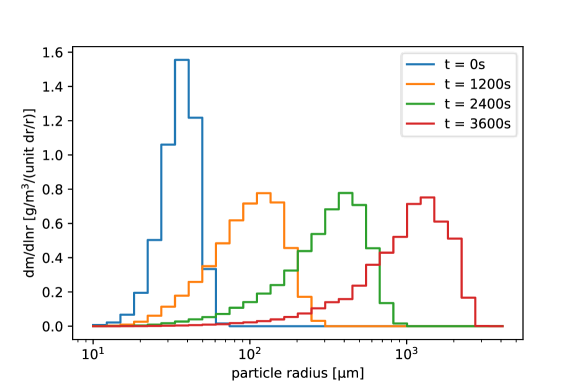
Figure 1: Sample plot generated with the code snippets included in the paper.

Usage examples

The PySDM examples are shipped in a separate package that can be installed with pip (pip install git+https://github.com/atmos-cloud-sim-uj/PySDM-examples.git) or conveniently experimented with using Colab or mybinder.org platforms (single-click launching badges included in the PySDM README file). The examples are based on setups from literature, and the package is structured using bibliographic labels (e.g., PySDM_examples.Shima_et_al_2009).

All examples feature a settings.py file with simulation parameters, a simulation.py file including logic analogous to the one presented in the code snippets above for handling composition of PySDM components using the Builder class, and a Jupyter notebook file with simulation launching code and basic result visualisation.

Box environment examples

The Box environment is the simplest one available in PySDM and the PySDM_examples package ships with two examples based on it. The first, is an extension of the code presented in the snippets in the preceding section and reproduces Fig. 2 from the seminal paper of Shima et al. (2009). Coalescence is the only process considered, and the probabilities of collisions of particles are evaluated using the Golovin additive kernel, which allows to compare the results with analytical solution of the Smoluchowski equation (included in the resultant plots).

The second example based on the Box environment, also featuring collision-only setup reproduces several figures from the work of Berry (1966) involving more sophisticated collision kernels representing such phenomena as the geometric sweep-out and the influence of electric field on the collision probability.

Adiabatic parcel examples

The Parcel environment shares the zero-dimensionality of Box (i.e., no particle physical coordinates considered), yet provides a thermodynamic evolution of the ambient air mimicking adiabatic displacement of an air parcel in hydrostatically stratified atmosphere. Adiabatic cooling during the ascent results in reaching supersaturation what triggers activation of aerosol particles (condensation nuclei) into cloud droplets through condensation. All examples based on the Parcel environment utilise the Condensation and AmbientThermodynamics dynamics.

The simplest example uses a monodisperse particle spectrum represented with a single super-droplet and reproduces simulations described in Arabas & Shima (2017) where an ascent-descent scenario is employed to depict hysteretic behaviour of the activation/deactivation phenomena.

A polydisperse lognormal spectrum represented with multiple super-droplets is used in the example based on the work of Yang et al. (2018). Presented simulations involve repeated ascent-descent cycles and depict the evolution of partitioning between activated and unactivated particles. Similarly, polydisperse lognormal spectra are used in the example based on Lowe et al. (2019), where additionally each lognormal mode has a different hygroscopicity. The Lowe et al. (2019) example additionally features representation of droplet surface tension reduction by organics.

Finally, there are two examples featuring adiabatic parcel simulations involving representation of the dynamics of chemical composition of both ambient air and the droplet-dissolved substances, in particular focusing on the oxidation of aqueous-phase sulfur. The examples reproduce the simulations discussed in Kreidenweis et al. (2003) and in Jaruga & Pawlowska (2018).

Kinematic (prescribed-flow) examples

Coupling of PySDM with fluid-flow simulation is depicted with both 1D and 2D prescribed-flow simulations, both dependent on the PyMPDATA package (Bartman et al., 2021) implementing the MPDATA advection algorithm. For a review on MPDATA, see e.g., Smolarkiewicz (2006).

Usage of the kinematic_1d environment is depicted in an example based on the work of Shipway & Hill (2012), while the kinematic_2d environment is showcased with a Jupyter notebook featuring an interactive user interface and allowing studying aerosol-cloud interactions in drizzling stratocumulus setup based on the work of Arabas et al. (2015).

Figure 2 presents a snapshot from the 2D simulation described in detail in Arabas et al. (2015) and works cited therein. Each plot depicts a 1.5 km by 1.5 km vertical slab of an idealised atmosphere in which a prescribed single-eddy non-divergent flow is forced (updraft in the left-hand part of the domain, downdraft in the right-hand part). The left plot shows the distribution of aerosol particles in the air. The upper part of the domain is covered with a stratocumulus-like cloud which formed on the aerosol particles above the flat cloud base at the level where relative humidity goes above 100%. Within the cloud, the aerosol concentration is thus reduced. The middle plot depicts the sizes of particles. Particles larger than 1 micrometre in diameter are considered as cloud droplets, particles larger than 50 micrometres in diameter are considered as drizzle (unlike in bin or bulk models, such categorisation is employed for analysis only and not within the particle-based model formulation). Concentration of drizzle particles forming through collisions is depicted in the right panel. A rain shaft forms in the right part of the domain where the downward flow direction amplifies particle sedimentation. Precipitating drizzle drops collide with aerosol particles washing out the sub-cloud aerosol. Most of the drizzle drops evaporate before reaching the bottom of the domain depicting the virga phenomenon and the resultant aerosol resuspension.

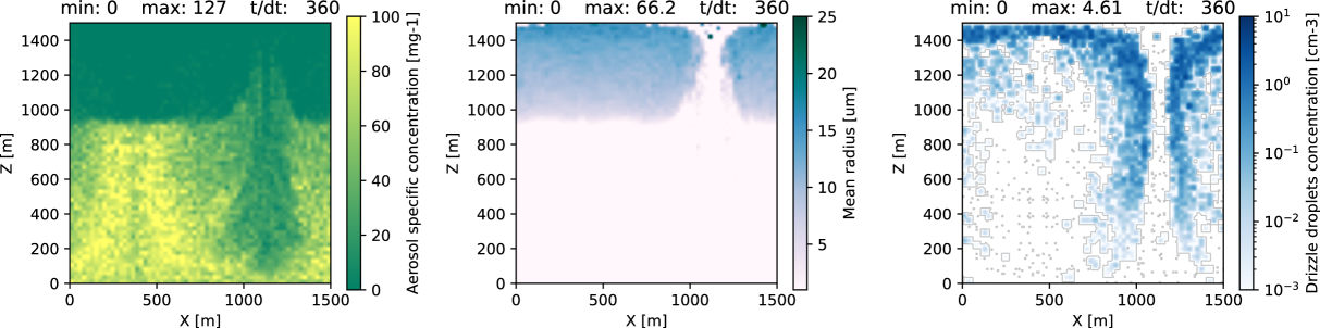
Figure 2: Results from a 2D prescribed-flow simulation using the Arabas et al. (2015) example.

Selected relevant recent open-source developments

The SDM algorithm implementations are part of the following open-source packages (of otherwise largely differing functionality):

• libcloudph++ in C++ (Arabas et al., 2015; Jaruga & Pawlowska, 2018) with Python bindings (Jarecka et al., 2015);

• SCALE-SDM in Fortran, (Sato et al., 2018);

• PALM LES in Fortran, (Maronga et al., 2020);

• LCM1D in Python/C, (Unterstrasser et al., 2020);

• Pencil Code in Fortran, (Brandenburg et al., 2021);

• NTLP in Fortran, (Richter et al., 2021).

• superdroplet in Python (Cython and Numba), C++, Fortran and Julia
  (https://github.com/darothen/superdroplet);

List of links directing to SDM-related files within the above projects’ repositories is included in the PySDM README file.

Python packages for solving the dynamics of aerosol particles with discrete-particle (moving-sectional) representation of the size spectrum include (both depend on the Assimulo package for solving ODEs):

• pyrcel, (Rothenberg & Wang, 2017);

• PyBox, (Topping et al., 2018).

Summary

The key goal of the reported endeavour was to equip the cloud modelling community with a solution enabling rapid development and paper-review-level reproducibility of simulations (i.e., technically feasible without contacting the authors and possible to be set up within minutes) while being free from the two-language barrier commonly separating prototype and high-performance research code. The key advantages of PySDM stem from the characteristics of the employed Python language which enables high performance computational modelling without trading off such features as:

succinct syntax

– the snippets presented in the paper are arguably close to pseudo-code;

portability

depicted in PySDM with continuous integration Linux, macOS and Windows;

interoperability

depicted in PySDM with Matlab and Julia usage examples requireing minimal amount of biding-specific code;

multifaceted ecosystem

depicted in PySDM with one-click execution of Jupyter notebooks on mybinder.org and colab.research.google.com platforms;

availability of tools for modern hardware

depicted in PySDM with the GPU backend.

PySDM together with a set of developed usage examples constitutes a tool for research on cloud microphysical processes, and for testing and development of novel modelling methods. PySDM is released under the GNU GPL v3 license.

Author contributions

PB had been the architect and lead developer of PySDM v1 with SA taking the role of main developer and maintainer over the time. PySDM 1.0 release accompanied PB’s MSc thesis prepared under the mentorship of SA. MO contributed to the development of the condensation solver and led the development of relevant examples. GŁ contributed the initial draft of the aqueous-chemistry extension which was refactored and incorporated into PySDM under guidance from AJ. KG and BP contributed to the GPU backend. CS and AT contributed to the examples. OB contributed the VTK exporter. The paper was composed by SA and PB and is partially based on the content of the PySDM README file and PB’s MSc thesis.

References

Arabas, S., Jaruga, A., Pawlowska, H., & Grabowski, W. W. (2015). libcloudph++ 1.0: A single-moment bulk, double-moment bulk, and particle-based warm-rain microphysics library in C++. Geosci. Model Dev. https://doi.org/10.5194/gmd-8-1677-2015

Arabas, S., & Shima, S. (2017). On the CCN (de)activation nonlinearities. Nonlin. Process. Geophys. https://doi.org/10.5194/npg-24-535-2017

Bartman, P., & Arabas, S. (2021). On the design of Monte-Carlo particle coagulation solver interface: A CPU/GPU super-droplet method case study with PySDM. ArXiv e-Prints. http://arxiv.org/abs/2101.06318

Bartman, P., Banaśkiewicz, J., Drenda, S., Manna, M., Olesik, M., Rozwoda, P., Sadowski, M., & Arabas, S. (2021). PyMPDATA v1: Numba-accelerated implementation of MPDATA with examples in Python, Julia and Matlab. https://pypi.org/p/PyMPDATA

Berry, E. X. (1966). Cloud droplet growth by collection. J. Atmos. Sci. https://doi.org/1520-0469(1967)024%3C0688:CDGBC%3E2.0.CO;2

Brandenburg, A., Johansen, A., Bourdin, P. A., Dobler, W., Lyra, W., Rheinhardt, M., Bingert, S., Haugen, N. E. L., Mee, A., Gent, F., Babkovskaia, N., Yang, C.-C., Heinemann, T., Dintrans, B., Mitra, D., Candelaresi, S., Warnecke, J., Käpylä, P. J., Schreiber, A., … Qian, C. (2021). The pencil code, a modular MPI code for partial differential equations and particles: Multipurpose and multiuser-maintained. J. Open Source Soft. https://doi.org/10.21105/joss.02807

Jarecka, D., Arabas, S., & Del Vento, D. (2015). Python bindings for libcloudph++. ArXiv e-Prints. http://arxiv.org/abs/1504.01161

Jaruga, A., & Pawlowska, H. (2018). libcloudph++ 2.0: Aqueous-phase chemistry extension of the particle-based cloud microphysics scheme. Geosci. Model Dev. https://doi.org/10.5194/gmd-11-3623-2018

Kreidenweis, S. M., Walcek, C. J., Feingold, G., Gong, W., Jacobson, M. Z., Kim, C. H., Liu, X., Penner, J. E., Nenes, A., & Seinfeld, J. H. (2003). Modification of aerosol mass and size distribution due to aqueous‐phase SO₂ oxidation in clouds: Comparisons of several models. J. Geophys. Res. https://doi.org/10.1029/2002JD002673

Lam, S. K., Pitrou, A., & Seibert, S. (2015). Numba: A LLVM-based python JIT compiler. Proceedings of the Second Workshop on the LLVM Compiler Infrastructure in HPC. https://doi.org/10.1145/2833157.2833162

Lowe, S. J., Partridge, D. G., Davies, J. F., Wilson, K. R., Topping, D., & Riipinen, I. (2019). Key drivers of cloud response to surface-active organics. Nature Comm. https://doi.org/10.1038/s41467-019-12982-0

Maronga, B., Banzhaf, S., Burmeister, C., Esch, T., Forkel, R., Fröhlich, D., Fuka, V., Gehrke, K., Geletič, J., Giersch, S., Gronemeier, T., Groß, G., Heldens, W., Hellsten, A., Hoffmann, F., Inagaki, A., Kadasch, E., Kanani-Sühring, F., Ketelsen, K., & Raasch, S. (2020). Overview of the PALM model system 6.0. Geosci. Model Dev. https://doi.org/10.5194/gmd-13-1335-2020

Morrison, H., Lier-Walqui, M. van, Fridlind, A. M., Grabowski, W. W., Harrington, J. Y., Hoose, C., Korolev, A., Kumjian, M. R., Milbrandt, J. A., Pawlowska, H., Posselt, D. J., Prat, O. P., Reimel, K. J., Shima, S., Diedenhoven, B. van, & Xue, L. (2020). Confronting the challenge of modeling cloud and precipitation microphysics. J. Adv. Model. Earth Syst. https://doi.org/10.1029/2019MS001689

Richter, D. H., MacMillan, T., & Wainwright, C. (2021). A Lagrangian cloud model for the study of marine fog. Boundary-Layer Meteorol. https://doi.org/10.1007/s10546-020-00595-w

Rothenberg, D., & Wang, C. (2017). An aerosol activation metamodel of v1.2.0 of the pyrcel cloud parcel model: Development and offline assessment for use in an aerosol–climate model. Geosci. Model. Dev. https://doi.org/10.5194/gmd-10-1817-2017

Sato, Y., Shima, S., & Tomita, H. (2018). Numerical convergence of shallow convection cloud field simulations: Comparison between double‐moment Eulerian and particle‐based Lagrangian microphysics coupled to the same dynamical core. J. Adv. Model. Earth Syst. https://doi.org/10.1029/2018MS001285

Shima, S., Kusano, K., Kawano, A., Sugiyama, T., & Kawahara, S. (2009). The super‐droplet method for the numerical simulation of clouds and precipitation: A particle‐based and probabilistic microphysics model coupled with a non‐hydrostatic model. Q. J. Royal Meteorol. Soc. https://doi.org/10.1002/qj.441

Shipway, B. J., & Hill, A. A. (2012). Diagnosis of systematic differences between multiple parametrizations of warm rain microphysics using a kinematic framework. Q. J. Royal Meteorol. Soc. https://doi.org/10.1002/qj.1913

Smolarkiewicz, P. K. (2006). Multidimensional positive definite advection transport algorithm: An overview. Int. J. Numer. Methods Fluids. https://doi.org/doi:10.1002/fld.1071

Topping, D., Connolly, P., & Reid, J. (2018). PyBox: An automated box-model generator for atmospheric chemistry and aerosol simulations. J. Open Source Soft. https://doi.org/10.21105/joss.00755

Unterstrasser, S., Hoffmann, F., & Lerch, M. (2020). Collisional growth in a particle-based cloud microphysical model: Insights from column model simulations using LCM1D (v1.0). Geosci. Model Dev. https://doi.org/10.5194/gmd-13-5119-2020

Yang, F. (2020). ThrustRTC: CUDA tool set for non-C++ languages that provides similar functionality like Thrust, with NVRTC at its core. In GitHub repository. GitHub. https://github.com/fynv/thrustrtc

Yang, F., Kollias, P., Shaw, R. A., & Vogelmann, A. M. (2018). Cloud droplet size distribution broadening during diffusional growth: Ripening amplified by deactivation and reactivation. Atmos. Chem. Phys. https://doi.org/10.5194/acp-18-7313-2018