Spectral Dependence

Abstract

This paper presents a general framework for modeling dependence in multivariate time series. Its fundamental approach relies on decomposing each signal in a system into various frequency components and then studying the dependence properties through these oscillatory activities. The unifying theme across the paper is to explore the strength of dependence and possible lead-lag dynamics through filtering. The proposed framework is capable of representing both linear and non-linear dependencies that could occur instantaneously or after some delay (lagged dependence). Examples for studying dependence between oscillations are illustrated through multichannel electroencephalograms. These examples emphasized that some of the most prominent frequency domain measures such as coherence, partial coherence, and dual-frequency coherence can be derived as special cases under this general framework. This paper also introduces related approaches for modeling dependence through phase-amplitude coupling and causality of (one-sided) filtered signals.

1 Introduction

Multivariate time series data, sets of a discretely sampled sequence of observations, are the natural approach for analyzing phenomena that display simultaneous, interacting, and time-dependent stochastic processes. As a consequence, they are actively studied in a wide variety of fields: environmental and climate science [1, 2, 3, 4, 5, 6], finance [7, 8, 9, 10, 11, 12], computer science and engineering [13, 14, 15, 16, 17, 18], public health [19, 20, 21, 22, 23], and neuroscience [24, 25, 26, 27, 28, 29, 30, 31, 32, 33, 34, 35, 36, 37, 38, 39]. Considering the inherent complexity of those studied phenomena, one of the most common challenges and tasks is identifying and explaining the interrelationship between the various components of the multivariate data. Thus, the purpose of this paper is to provide a summary of the various characterizations of dependence between the elements of a multivariate time series. The emphasis will be on the spectral measures of dependence which essentially examines the cross-relationships between the various oscillatory activities in these signals. These measures will be demonstrated, for the most part, through the oscillations derived from linear filtering.

Suppose ${\bf X}(t)=[X_{1}(t),\ldots,X_{P}(t)]^{\prime}$ is a multivariate time series with $P$ components. This abstraction is capable of providing a general framework that describes a broad range of scenarios and phenomena. For instance, in environmental studies, components $X_{1},\ldots,X_{P}$ could represent recordings from various air pollution sensors at a fixed location. Similarly, the same framework could describe wind velocity recordings at $P$ different geographical locations. In a neuroscience experiment, a component $X_{i}$ could be the measurement of brain electrical, or hemodynamic, activity from a specific sensor (electrode) which is placed either on the scalp or on the surface of the brain cortex. The key question that we will address through various statistical models and data analysis tools is to understand the a) nature of marginal dependence between $X_{p}(t)$ and $X_{q}(t)$ or b) between $X_{p}(t)$ and $X_{q}(t)$ conditional on the other components in the data.

This work is largely motivated from a neuroscience perspective. The brain circuitry can be conceived as the integration of a sensory, motor, and cognitive system that receives, processes, and reacts to external impulses or internal auto-regulation activities [40, pp. 80-91]. Communication and feedback between those structures enable brain functions. For instance, memory is believed to rely on the hippocampus because it is at the center in the signal flow from and to the cortical areas, such as the orbitofrontal cortex, olfactory bulb, and superior temporal gyrus [41, 42, p. 160-165]. From a macro perspective, those memory flows also imply a high activity in the temporal brain region [42, p. 164]. From an analytic perspective, these signal interactions can be studied as undirected dependencies (functional connectivity) $X_{p}(t)\Leftrightarrow X_{q}(t)$; or directed, or causal, networks (effective connectivity) $X_{p}(t)\Rightarrow X_{q}(t)\,\wedge\,X_{q}(t)\Rightarrow X_{p}(t)$. Additionally, current imaging techniques allow us to understand those interactions at different biological levels: (a.) through neuron hemoglobin changes (energy consumption) using functional magnetic resonance imaging (fMRI) or functional near-infrared spectroscopy (fNIRS); (b.) through measurements of the electrical activity at the scalp, (electroencephalogram, EEG), at the cortical surface (electrocorticogram, ECoG), or in the extracellular environment (local field potentials, LFPs).

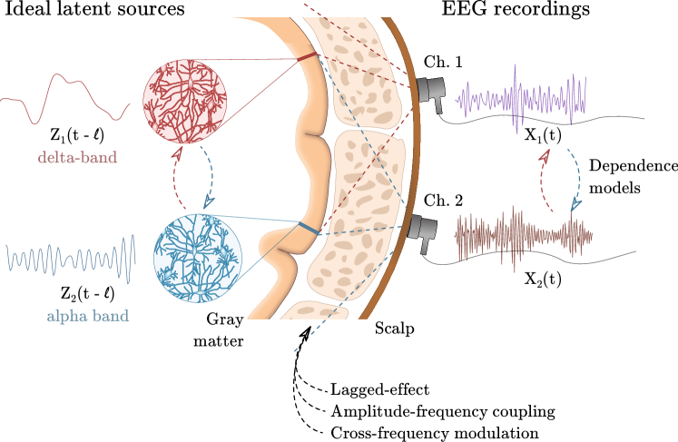
Figure 1: Abstraction of dependence in biomedical signals. It is assumed that hypothetical latent sources could generate neural oscillations (with their own frequency characteristics) that can interact among them before being recorded as the scalp. Different abstractions that model the sources’ interactions and the mixing models are explained in this paper.

We should emphasize that there are several models that aim to represent the different types of dependence (Figure 1). The most common measure of dependence is cross-covariance (or cross-correlation). In the simple case where ${\mathbb{E}}\left[X_{p}(t)\right]=0$ and $\mbox{Var}\left[X_{p}(t)\right]=1$ for all $p=1,\ldots,P$ and all time $t$, then the cross-correlation between $X_{p}$ and $X_{q}$ is

$$\rho_{pq}(0)={\mathbb{E}}\left[X_{p}(t)X_{q}(t)\right]=\int u_{p}u_{q}f_{pq}(u_{p},u_{q})\;du_{p}du_{q}$$ (1)

where $f_{pq}(u_{p},u_{q})$ is the joint probability density function of $(X_{p}(t),X_{q}(t))$ and the integral is evaluated globally over the entire support of $(X_{p}(t),X_{q}(t))$. Cross-correlation provides a simple metric that measures the linear synchrony between a pair of components across the entire support of their joint distribution. When $|\rho_{pq}(0)|$ has a value close to $1$, we conclude that there is a strong linear dependence between $X_{p}$ and $X_{q}$. It is obvious that cross-correlation does not completely describe the nature of dependence between $X_{p}$ and $X_{q}$. First, dependence goes beyond linear associations, and hence this paper addresses some types of non-linear dependence between components. Second, dependence may vary across the entire support. That is, the association between $X_{p}$ and $X_{q}$ at the "center" of the distribution may be different from its "tails" (e.g., extrema). Third, since time series data can be viewed as superpositions of sine and cosine waveforms with random amplitudes, the natural aim is to identify the specific oscillations that drive the linear relationship. This will be the main focus of the models and methods that will be covered in this paper.

To consider spectral measures of dependence (i.e., dependence between oscillatory components), our starting point will be the Cramér representation of stationary time series. Under stationarity, we can decompose both $X_{p}$ and $X_{q}$ into oscillations at various frequency bands. The key elements of the Cramér representation are the Fourier basis waveforms $\bigl{\{}\exp(i2\pi\omega t),\omega\in(-\frac{1}{2},\frac{1}{2})\bigr{\}}$ and the associated random coefficients $\{dZ(\omega)\}$ which is an orthogonal increment random process that satisfies ${\mathbb{E}}\left[dZ(\omega)\right]=0$ and $\mathop{\rm{\mathbb{C}}ov}\nolimits(dZ(\omega),dZ(\omega^{\prime}))\neq 0$ for $\omega\neq\omega^{\prime}$. The Cram’er representation for $(X_{p}(t),X_{q}(t))$ is given by

$$\left(\begin{matrix}X_{p}(t)\\ X_{q}(t)\\ \end{matrix}\right)= \left(\begin{matrix}\exp(i2\pi\omega t)\,dZ_{p}(\omega)\\ \exp(i2\pi\omega t)\,dZ_{q}(\omega)\end{matrix}\right)$$ (2)

and $X_{q}$ by examining the nature of synchrony between the $\omega$-oscillation in $X_{p}$ and the $\omega$-oscillation in $X_{q}$ which are, respectively, $\exp(i2\pi\omega t)dZ_{p}(\omega)$ and $\exp(i2\pi\omega t)dZ_{q}(\omega)$. This idea will be further developed in the next sections of this paper. We emphasize that stationarity assumption can be held in resting-state conditions [43, p. 188] or within reasonable short time intervals [44, p. 20].

Most brain signals exhibit non-stationary behavior, which may be reflected changes in either (a.) the mean level, or (b.) the variance at some channels, or (c.) the cross-covariance structure between some pairs of channels. Note here that (a.) is a condition on the first moment while (b.) and (c.) are conditions on the second moment. Moreover, (a.) and (b.) are properties within a channel, while (c.) is a property that describes dependence between a pair of channels. There is no measure that completely describes the nature of dependence between channels. The most common pair of measures consists of the cross-covariance and cross-correlation, whose equivalent measures in the frequency domain are the cross-spectrum and cross-coherence, respectively. This paper will focus on the frequency domain measures and thus dig deeper into being able to identify the oscillations that drive the dependence between a pair (or group) of channels. Under non-stationarity, the dependence structure can change over time. Our approach here is to slide a localized window across time and estimate the spectral properties within each window. This approach is proposed in [45] and then reformulated in [46] to establish an asymptotic framework for demonstrating the theoretical properties of the estimators.

2 EEG spectral characteristics

To illustrate the various spectral dependence measures, we shall focus on the analysis of EEG signals. EEG is a noninvasive imaging technique that collects electrical potential at the scalp gathered from synchronized responses of groups of neurons (“signal sources”) [47, p. 4] [43, p. 555] that are perpendicular to the scalp and dynamically organized in neighborhoods with scales of a few centimeters [48, p. 5]. Naturally, EEG is affected by the volume conduction of the signals over tissue and skull [49, p. 144]. Despite its limitations, the portability and inexpensiveness allow the integration of EEG in clinical settings and cognitive experiments that require naturalistic environments (in contrast, fMRI experiments require the participants to be in a supine position in a restricted space). In addition, the EEG high temporal resolution enables to capture the temporal dynamics of the neuronal activity. Therefore, through spatial, temporal, and morphological EEG patterns, some conditions can be diagnosed [48, p.3, 19-22]. For instance, a specific metric obtained from EEG frequency properties measured on the channel Cz is considered an FDA-approved clinical method to assess attention deficit hyperactivity disorder (ADHD) [50]. Thus, EEGs have been extensively used in cognitive neuroscience, neurology, and psychiatry to study the neurophysiological basis of cognition and neuropsychiatric disorders: motor abilities [51], anesthetic similarities with comma [52], encephalopathy [53], schizophrenia [25], addictions [54], spectrum autism disorder [54, 55], depression [56, 57, 58], and ADHD [50, 59]. Here, we will illustrate some methods that characterize the dynamics of the inter-relationships between the activity measured at different channels.

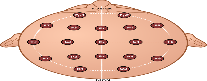
Figure 2: Electrode positioning in the 10-20 standard layout.

In this paper, we use the EEG dataset related to a mental health disorder collected by Nasrabadi et al. [60]. This data comprises EEGs, sampled at 128Hz, from 60 children with attention deficit hyperactivity disorder (ADHD) and 60 children with no registered psychiatric disorder as a control group. These electrical recordings were collected from 19 channels evenly distributed on the head in the 10-20 standard layout (Figure 2). Average recording from both ear lobes (A1 and A2) was used as electrode references. The experiment was intended to show potential differences in the brain response under visual attention task [60, 61, 59]. Therefore, the 120 participants were exposed to a series of images that they should count. The number of images in each set ranged from 5 to 16 with a reasonable size in order to allow them to be recognizable and countable by the children. Each collection of pictures was displayed without interruptions in order to prevent distraction from the subjects.

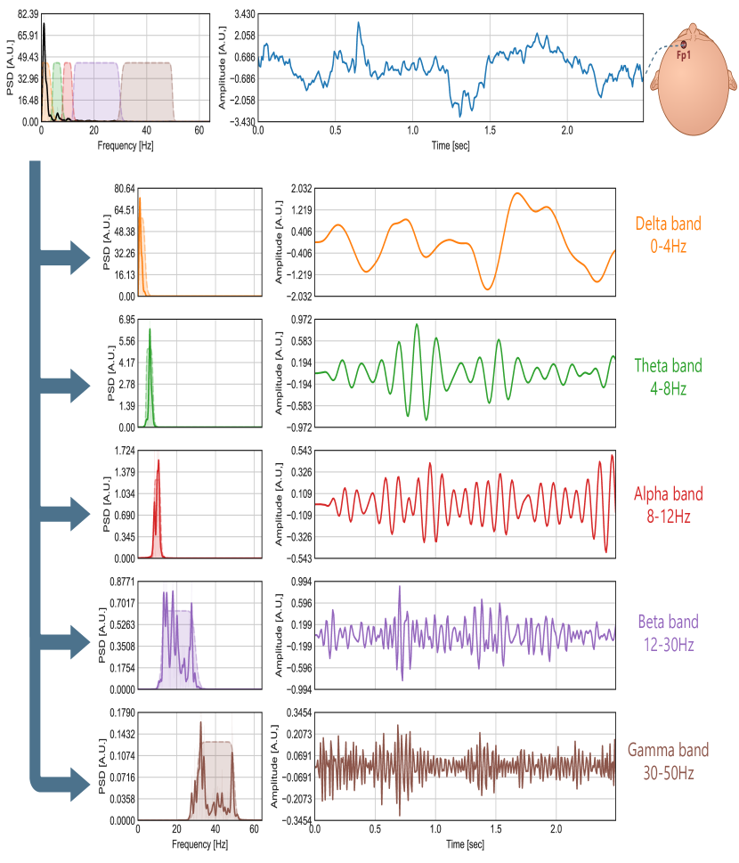
Figure 3: Frequency decomposition of an EEG, collected at channel Fp1, into the five brain rhythms: delta, theta, alpha, beta and gamma.

Prior to analysis, EEGs undergo significant pre-processing steps. These procedures are not unique to EEGs, or brain signals, as most data often need some cleaning before statistical modeling. Several attempts have been performed to standardize those pre-processing steps [62, 63, 64, 65, 66]. In general, pre-processing aims to increase the quality of the recorded signal by [67]: (a.) removing the effect of the electrical line (electrical interference at 50Hz or 60Hz due to the electrical source); (b.) removing artifacts due to eye movements, eye blinks or muscular movements; (c.) detecting, removing or repairing bad quality channels; (d.) filter non-relevant signal components; and (e.) re-referencing the signal to improve topographical localization. In this scenario, filtering is a crucial step that removes portions of the signal that could not be related to cognitive or physiological processes, such as extremely high-frequency components. In this dataset, we applied a band-pass filter on the frequency interval (0.0-70.0) Hz and segmented the signal into the main “brain rhythms” 43, p.610; 48, p. 33-34, 169-170, 413-414; 49, p. 12: frequency range into the delta band: (0.5, 4.0) Hertz, theta band: (4.0, 8.0) Hz, alpha band: (8.0, 12.0) Hertz, beta band: (12.0, 30.0) Hertz, and gamma band: (30.0, 50.0) Hertz. A non-causal second-order Butterworth filter was used to perform this frequency filtering: Figure 3 shows an example of this decomposition where the shadow regions show the magnitude response of the applied filter. Finally, the EEGs are also often segmented into epochs of sixty seconds.

3 Coherence and Partial Coherence

In this section, we formally describe two of the most common measures of spectral dependence, namely, coherence and partial coherence. A formal description for these measures is derived under the context of the Cramér representation of weakly stationary processes. We also presented an alternative interpretation of these dependence metrics as the squared correlation between filtered signals. Finally, these measures are derived for the general case where the signals exhibit non-stationarity, e.g., under conditions where the dependence between signals may evolve over time.

3.1 Coherence and Correlation via the Fourier transform

Suppose that ${\bf X(t)}$ is a $P-$dimensional weakly stationary process with mean ${\mathbb{E}}{\bf X}(t)=\underline{0}$ for all time $t$ and sequence of covariance matrices $\left\{\Sigma(h),\ h=0,\pm 1,\pm 2,\ldots\right\}$ where $\Sigma(h)$ is defined by

$$\Sigma(h)=\mathop{\rm{\mathbb{C}}ov}\nolimits\left({\bf X}(t+h),{\bf X}(t)\right)={\mathbb{E}}\left({\bf X}(t+h){\bf X}^{\prime}(t)\right).$$

Here, we assume absolute summability (over lag $h$) of every element of $\Sigma(h)$. Let $\sigma_{pq}(h)$ be the $(p,q)$-th entry of the matrix $\Sigma(h)$. Then, $\sum_{h=-\infty}^{\infty}|\sigma_{pq}(u)|<\infty$ for all $(p,q)$. This condition will ensure that auto-correlation and cross-correlation decay sufficiently fast to $0$.

We need to highlight that there is a one-to-one relationship between the covariance matrix $\Sigma(h)$ and the spectral matrix via the Fourier transform. The spectral matrix, denoted ${\bf f}(\omega)$, is defined as

$${\bf f}(\omega)=\sum_{h=-\infty}^{\infty}\Sigma(h)\exp(-i2\pi\,\omega\,h)\quad\text{ where }\omega\in\Omega_{0}=\left(-0.5,0.5\right).$$

${\bf f}(\omega)$ is a $P\times P$ Hermitian semi-positive definite matrix.

From a univariate perspective, the matrix ${\bf f}(\omega)$ can be sufficient to describe the spectral properties of each one of their components. For instance, the auto-spectrum (univariate spectrum) of the $p$-th channel, which is denoted as $f_{pp}(\omega)$, can be obtained from the $(p,p)$-th entry of ${\bf f}(\omega)$.

In addition, the autocovariance sequence $\sigma_{pp}(h)$ can be derived from auto-spectrum $f_{pp}(\omega)$ via the inverse-Fourier transform

$$\sigma_{pp}(h)=\int_{\omega\in\Omega_{0}}f_{pp}(\omega)\,\exp\left(i2\pi\,\omega,h\right)\,d\omega.$$

Note that as a special case, when $h=0$, then $\sigma_{pp}(0)=\mbox{Var}\left(X_{p}(t)\right)$. This corollary provides the intuition that the auto-spectrum is decomposing the signal variance across all frequencies $\omega\in\Omega_{0}=(-0.5,0.5)$:

$$\sigma_{pp}(0)=\int_{\omega\in\Omega_{0}}f_{pp}(\omega)\,d\omega=\mbox{Var}\left(X_{p}(t)\right).$$ (3)

Now, we can introduce correlation as a dependence metric. Correlation between two components $X_{p}$ and $X_{q}$ at time lag $h$ is defined by

$$r_{p,q}(h)=\mathop{\rm{\mathbb{C}}or}\nolimits\left(X_{p}(t+h),X_{q}(t)\right)=\frac{\mathop{\rm{\mathbb{C}}ov}\nolimits\left(X_{p}(t+h),X_{q}(t)\right)}{\sqrt{\mbox{Var}X_{p}(t)\,\mbox{Var}X_{q}(t)}}=\frac{\sigma_{pq}(h)}{\sqrt{\sigma_{pp}(0)\,\sigma_{qq}(0)}}.$$

It is clear that $r_{p,q}(h)\in[-1,1]$ will reach its extreme value when one of the signals is proportional to the other. Thus, correlation $r_{p,q}(h)$ is known for being the simplest measure the quantifies the linear dependence, or synchrony, at a lag $h$ between the pair of time series.

Furthermore, the spectral matrix ${\bf f}(\omega)$ provides more information about the interactions of their components. For instance, it allows us to identify the cross-spectrum between any pair of components, $X_{p}$ and $X_{q}$, through its $(p,q)$-th entry. In a similar manner to the correlation, in the time domain, we can define another measure that quantifies the similarity between the simultaneous spectral response of $X_{p}$ and $X_{q}$. This metric is known as coherency, and it is formally defined as

$$\tau_{pq}(\omega)=\frac{f_{pq}(\omega)}{\sqrt{f_{pp}(\omega)f_{qq}(\omega)}}$$ (4)

However, it is more common to use a derived metric: the cross-coherence that is the square magnitude of the coherency:

$$\rho_{pq}(\omega)=\left|\tau_{pq}(\omega)\right|^{2}=\frac{\left|f_{pq}(\omega)\right|^{2}}{f_{pp}(\omega)f_{qq}(\omega)}.$$ (5)

Cross-coherence $\rho_{pq}(\omega)\in[0,1]$ will achieve its maximum value only when both compared time series have a proportional cross-frequency response.

3.2 Coherence and Correlation using the Cramér representation

We now define coherency and coherence in the robust framework of the Cramér representation (CR) as an alternative of the definitions based on the Fourier transform of the covariance matrix. The CR of a zero-mean $P-$dimensional weakly stationary process ${\bf X(t)}$ is given by

$${\bf X}(t)=\int_{-0.5}^{0.5}\exp\left(i2\pi\,\omega\,t\right)\,d{\bf Z}(\omega)$$

where $d{\bf Z}(\omega)=\left[dZ_{1}(\omega),\ldots,dZ_{P}(\omega)\right]^{\prime}$ is a vector of random coefficients associated with the Fourier waveform $\exp(i2\pi\omega t)$ for each of the $P$ components. Here, $\{d{\bf Z}(\omega)\}$ is a random process defined on $(-0.5,0.5)$ that satisfies ${\mathbb{E}}\left[d{\bf Z}(\omega)\right]=0$ for all frequencies $\omega$ and

$$\mathop{\rm{\mathbb{C}}ov}\nolimits\left(d{\bf Z}(\omega),d{\bf Z}(\omega^{\prime})\right) = \left\{\begin{array}[]{cc}0,&\omega\neq\omega^{\prime}\\ {\bf f}(\omega)d\omega,&\omega=\omega^{\prime}\end{array}\right.$$

From the above formulation, we note that the correlation and modulus-squared correlation with the coefficients are, in fact, coherency and coherence as they were defined in Equations 4 and  5:

$$\mathop{\rm{\mathbb{C}}or}\nolimits\left[d{\bf Z}_{p}(\omega),d{\bf Z}_{q}(\omega)\right] = \frac{f_{pq}(\omega)}{\sqrt{f_{pp}(\omega)f_{qq}(\omega}}$$

$$\left\|\mathop{\rm{\mathbb{C}}or}\nolimits\left[d{\bf Z}_{p}(\omega),d{\bf Z}_{q}(\omega)\right]\right\|^{2} = \frac{\left|f_{pq}(\omega)\right|^{2}}{f_{pp}(\omega)f_{qq}(\omega)}.$$

Recall that the CR represents a time series as a linear mixture of infinitely many sinusoidal waveforms (Fourier waveforms with random amplitudes). This perspective allows us to provide a different interpretation of the above-mentioned dependence metrics. Consider the components $X_{p}$ and $X_{q}$, both of them contain Fourier oscillations in a continuum of frequencies, and let us now focus only on the specific frequency $\omega$ in the two components:

$$X_{p,\omega}(t) = \exp\left(i2\pi\omega t\right)\,dZ_{p}(\omega)$$

$$X_{q,\omega}(t) = \exp\left(i2\pi\omega t\right)\,dZ_{q}(\omega).$$

Assuming that these random coefficients have zero mean, the variance at the $\omega$-oscillatory activity of $X_{p}$ is

$$\mbox{Var}\left[X_{p,\omega}(t)\right]=\left|\exp(i2\pi\,\omega\,t)\right|^{2}\mbox{Var}\left[dZ_{p}(\omega)\right].$$

Since the random coefficients $\left\{dZ_{p}(\omega)\right\}$ are uncorrelated across $\omega\in(-0.5,0.5)$, it follows that

$$\mbox{Var}\left[X_{p}(t)\right]=\int\mbox{Var}\left[X_{p,\omega}(t)\right]=\int\mbox{Var}\left[dZ_{p}(\omega)\right].$$

Based on this relationship, we can introduce an alternative interpretation of the spectral decomposition denoted along with Equation 3: the total variance of a weakly stationary signal $X_{p}$ at any time point can be viewed as an infinite sum of the variance of each of the random coefficients. Furthermore, we can think of the relationship between the variance of the random coefficients and the spectrum as follows

$$\mbox{Var}\left[dZ_{p}\left(\omega\right)\right]=f_{pp}\left(\omega\right)\,d\omega.$$

Now, let us study the relationship between the signals $X_{p}$ and $X_{q}$ as a function of the oscillations. The covariance between the $\omega-$oscillation in $X_{p}$ and the $\omega-$oscillation in $X_{q}$ is

$$\mathop{\rm{\mathbb{C}}ov}\nolimits\left[X_{p,\omega}(t),X_{p,\omega}(s)\right] = \exp\left(i2\pi\omega(t-s)\right)\,\mathop{\rm{\mathbb{C}}ov}\nolimits\left[dZ_{p}(\omega),dZ_{q}(\omega)\right].$$

Moreover, since $|\exp(i2\pi\omega t)|=1$ for all $t$, the variances of these respective $\omega$-oscillations are

$$\mbox{Var}\left[X_{p,\omega}(t)\right]=\mbox{Var}\left[dZ_{p}(\omega)\right]\quad{\mbox{and}}\quad\mbox{Var}\left[X_{q,\omega}(t)\right]=\mbox{Var}\left[dZ_{q}(\omega)\right].$$

In addition, the correlation between these $\omega$-oscillations is

$$\mathop{\rm{\mathbb{C}}or}\nolimits\left[X_{p,\omega}(t),X_{p,\omega}(s)\right]=\exp\left(i2\pi\omega(t-s)\right)\mathop{\rm{\mathbb{C}}or}\nolimits\left[dZ_{p}(\omega),dZ_{q}(\omega)\right]$$

and the respective modulus-squared correlation is given by

$$\left|\mathop{\rm{\mathbb{C}}or}\nolimits\left[X_{p,\omega}(t),X_{p,\omega}(s)\right]\right|^{2}=\left|\mathop{\rm{\mathbb{C}}or}\nolimits\left[dZ_{p}(\omega),dZ_{q}(\omega)\right]\right|^{2}$$

which is identical to the definition of coherence given in Equation 5.

In summary, it is possible to affirm that coherence between a pair of weakly stationary signals at frequency $\omega$ is the square-magnitude of the correlation between the $\omega$-oscillations of these signals.

3.3 Coherence and filtering

In practical EEG analysis, coherence between a pair of channels is defined and estimated at some frequency bands - rather than in a singleton frequency. The standard frequency bands are delta $(0.5,4.0)$ Hertz, theta $(4.0,8.0)$ Hertz, alpha $(8.0,12.0)$ Hertz, beta $(12.0,30.0)$ Hertz and gamma $(30.0,50.0)$ Hertz. This segmentation of the frequency axis has been widely accepted for many decades. However, there is a growing direction towards a more specific (narrower) frequency band analysis and a more data-adaptive approach to determining (a.) the number of frequency peaks, (b.) the location of these peaks, and (c.) the bandwidth associated with each one of them. This will be necessary for a finer differentiation between experimental conditions and patient diagnosis groups. The immediate task at hand is to point out the connection between linear filters and spectral and coherence estimation.

To estimate coherence, the first step is to apply a linear filter on time series components $X_{p}$ and $X_{q}$ so that the resulting filtered time series will have spectra whose power is concentrated around a pre-specified band $\Omega$. In essence, a $k$-th order linear frequency-filter is comprised of a set of coefficients $\left\{a_{0},\ldots,a_{K}\right\}$ and $\left\{b_{1},\ldots,b_{K}\right\}$ under the constraint $\sum_{k}|a_{k}|<\infty$ and $\sum_{k}|b_{k}|<\infty$. The filtered signal $y^{*}(t)$ is obtained as a linear combination of the previous values of the unfiltered time series $y(t),\ldots,y(t-K)$ and its previous values $y^{*}(t-1),\ldots,y^{*}(t-K)$:

$$y^{*}(t)=\sum_{k=0}^{M}b_{k}y(t-k)-\sum_{k=1}^{M}a_{k}y^{*}(t-k)$$ (7)

Filters with $a_{k}=0\,\forall k$ are known as finite impulse response (FIR) filters or infinite impulse response (IIR) filters when $\exists a_{k}\neq 0$ for some $k$. For an extensive analysis of linear time-invariant filtering, we refer to [68]. Here, we will focus on the FIR family of filters. Consider the filter so that $\left\{c_{k},k=0,\pm 1,\pm 2,\ldots\right\}$. A one-sided linear filter will be used to examine causality between the different oscillations, a further discussion about the reasons behind this condition is given in Section 5.4.

The Fourier transform of the sequence of FIR filter coefficients $\{c_{j}\}$ is

$$C\left(\omega\right)=\sum_{k}\ c_{k}\exp(-i2\pi\omega\,k)$$

which is called the frequency response function so that $|C(\omega)|$. The set of filter coefficients are selected so that $C(\omega)$ has a peak that is concentrated in the neighborhood of the frequency band $\Omega$ (band-pass region). In the frequency intervals outside of $\Omega$ (stop-band region),$|C(\omega)|$ is expected to has relatively small values. Thus, to extract the component of $X_{p}$ and $X_{q}$ that is associated with the $\Omega$-oscillation, we apply the linear filter $\left\{c_{j},j=0,\pm 1,\pm 2,\ldots\right\}$ to obtain the convolution

$$X_{p,\Omega}(t) = \sum_{j=-\infty}^{\infty}c_{j}X_{p}(t-j)$$

$$X_{q,\Omega}(t) = \sum_{j=-\infty}^{\infty}c_{j}X_{q}(t-j).$$

The auto-spectra of each filtered series, $\{X_{p,\Omega}\}$ and $\{X_{q,\Omega}\}$, is

$$f_{pp,\Omega}(\omega) = \left|C(\omega)\right|^{2}\,f_{pp}(\omega)$$

$$f_{qq,\Omega}(\omega) = \left|C(\omega)\right|^{2}\,f_{qq}(\omega),$$

respectively, which has spectral power attenuated outside of the band $\Omega$.

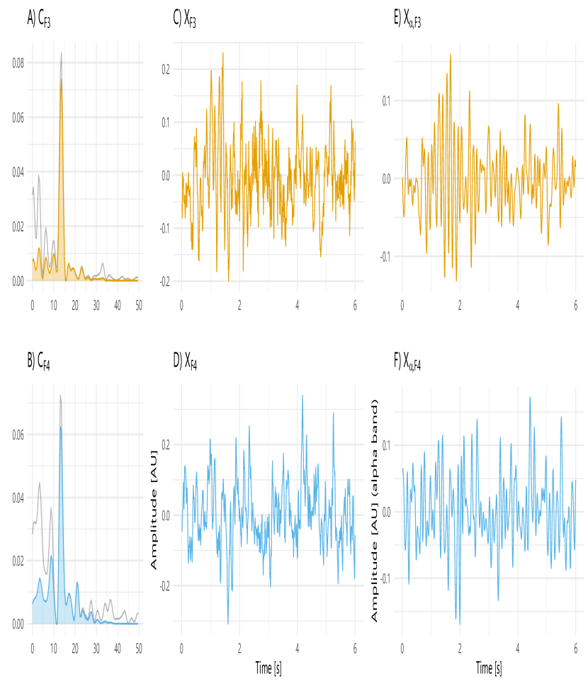
Figure 4: Alpha-filtering of EEG signals in channels F3 and F4: A,B) Power spectrum density $C_{F4}$ and $C_{F3}$ after applying a band-pass filter. Note that the power is concentrated only in the interval 8-12Hz. The gray line in the background corresponds to the unfiltered spectra.C,D) Signals $X_{F3}$ and $X_{F4}$ without before filtering; and E.F) Alpha waves in both channels: $X_{F3,\alpha}$ and $X_{F4,\alpha}$.

Example 1 (EEG example).

Recall the EEG-ADHD dataset described in Section 2. Let us focus in the signals recorded at channels F3 and F4, collected from the control subject S041. We denoted them by $X_{p}$ and $X_{q}$ (Figure 5.C-D). These biomedical signals are sampled at $128$ Hertz and with a 60-second epoch. In consequence, the total number of time points available for the analysis is $T=128\times 60=7680$.

We extract the alpha-band component ($\Omega=8-12$Hertz) using a 10-th order FIR band-pass filter defined by the coefficients:

$$\left\{c_{i}\right\} = \left\{-0.0272,-0.0468,-0.0423,0.0771,0.2677,\right.$$

$$\left.0.3629,0.2677,0.0771,-0.0423,-0.0468,-0.0272\right\}$$

The filtering results are depicted in Figure 5.E-F with the spectrum after the filtering process in Figure 5.A-B.

Figure 5: Linear relationships between the channels F3 and F4: A) Scatterplot of the unfiltered signals, with a correlation of 0.033. B-F) Scatterplots of alpha-filtered channels at different lags: -40, -20, 0, 20, and 40. Note that lags are denoted from reference to F3 ($X_{p}$).Thus, negative lags imply that F4 is leading F3 during the correlation estimation. G) Cross-correlation as a function of the lags. The maximum cross-correlation (0.138) is located at lag 1.

The next step is to study the dependence between the time series $X_{p}$ and $X_{q}$ through their filtered components. In practice, dependence can be examined at various frequency bands but in this example, we focus only on the alpha band for illustration purposes.

From Ombao, H. and Van Bellegem. S. [69], we can estimate the band-coherence, i.e., the coherence between the two EEG channels, $X_{p}$ the estimated coherence between the EEG channels $X_{p}$ and $X_{q}$ at the alpha-band is

$$\rho_{p,q}(\alpha)\propto\max_{\ell}\left|\sum_{t}X_{p,\alpha}(t)\,X_{q,\alpha}(t-\ell)\right|^{2}.$$ (8)

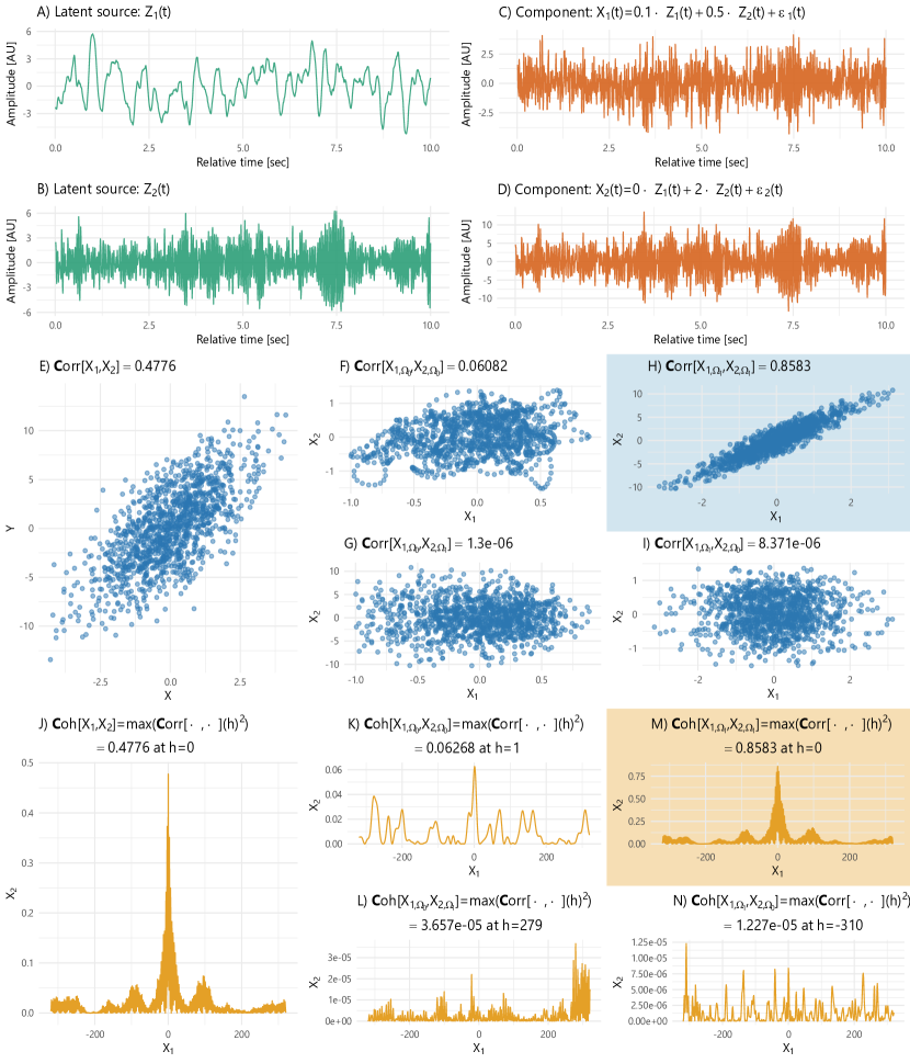
Figure 6: Simulated example 2: system with an instantaneous mixture with latent sources ($Z_{1}(t)$, $Z_{3}(t)$) and mixed components ($X_{1}(t)$, $X_{2}(t)$). Note the differences in the correlation between the unfiltered, and the $\Omega_{0}$- and $\Omega_{1}$-filtered components. $\mathop{\rm{\mathbb{C}}or}\nolimits\left[X_{1}(t),X_{2}(t)\right]=0.4776$ while $\mathop{\rm{\mathbb{C}}or}\nolimits\left[X_{\Omega 0}(t),X_{\Omega 0}(t)\right]=0.0608$ and $\mathop{\rm{\mathbb{C}}or}\nolimits\left[X_{\Omega 1}(t),X_{\Omega 1}(t)\right]=0.8583$.

Example 2 (Contemporaneous mixture).

We now illustrate that coherence gives information beyond cross-correlation (or the square cross-correlation). Consider the setting where there are two latent sources $Z_{1}$ and $Z_{2}$ where $Z_{1}$ is a high-frequency source and $Z_{2}$ is a low-frequency source. Define the observed time series $X_{1}$ and $X_{2}$ to be mixtures of these two sources, e.g.,

$$\left(\begin{matrix}X_{1}(t)\\ X_{2}(t)\end{matrix}\right) = \left(\begin{matrix}c_{11}&c_{12}\\ c_{21}&c_{22}\end{matrix}\right)\ \ \left(\begin{matrix}Z_{1}(t)\\ Z_{2}(t)\end{matrix}\right)\ +\ \left(\begin{matrix}\epsilon_{1}(t)\\ \epsilon_{2}(t)\end{matrix}\right).$$ (9)

Suppose that $c_{21}=0$ and the other entries of the mixing matrix are all non-zero. This implies that $X_{1}$ contains both low-frequency component $Z_{1}$ and high-frequency component $Z_{2}$. However, $X_{2}$ contains only the high-frequency component $Z_{2}$. Thus, it is the high-frequency component that drives the dependence between $X_{1}$ and $X_{2}$. The scatterplot of $X_{2}(t)$ vs $X_{1}(t)$ in Figure 6.E shows that these two time series are correlated and the sample cross-correlation is computed to be 0.4776. However, correlation is limited in the information it can convey about the relationship between a pair of signals. For instance, it does not indicate what frequency band(s) drive that relationship.

To now investigate deeper the relationship between $X_{1}$ and $X_{2}$, we apply a low-pass filter (on band $\Omega_{0}$) and a high-pass filter (on band $\Omega_{1}$) and denote these filtered signals to be

$$X_{1,\Omega_{0}}(t),\ X_{1,\Omega_{1}}(t),\ X_{2,\Omega_{0}}(t),\ X_{2,\Omega_{1}}(t).$$

Under stationarity, the random coefficients in the Cramér representation are uncorrelated across frequencies (i.e., $\mathop{\rm{\mathbb{C}}ov}\nolimits[dZ_{1}(\omega),dZ_{2}(\omega^{\prime})]=0$ when $\omega\neq\omega^{\prime}$). Thus,

$$\mathop{\rm{\mathbb{C}}ov}\nolimits[X_{1,\Omega_{0}}(s),X_{2,\Omega_{1}}(t)] = 0$$

$$\mathop{\rm{\mathbb{C}}ov}\nolimits[X_{1,\Omega_{1}}(s),X_{2,\Omega_{0}}(t)] = 0.$$

For some non-stationary processes, there could be possible linear and non-linear dependence between different frequency bands. For the moment, we focus only on the correlation between the low-frequency components $X_{1,\Omega_{0}}(s)$ and $X_{2,\Omega_{0}}(t)$ and the high-frequency components $X_{1,\Omega_{1}}(s)$ and $X_{2,\Omega_{1}}(t)$. The lag-$0$ scatterplots are shown in 6.F-I. It is clear here that the linear relationship between the low-frequency components is weaker than the dependence on high-frequency components. This was to be expected from the data generating model in Equation 2, which specifies that $X_{1}$ and $X_{2}$ both share the common high-frequency latent source. Assuming that the sample mean of these oscillations are all $0$, then the coherence estimate at the low-frequency band is the squared cross-correlation between the $X_{1,\Omega_{0}}$ and $X_{2,\Omega_{0}}$, i.e.,

$$\widehat{\rho}_{12}(\Omega_{0})=\frac{\left\{\sum_{t=1}^{T}(X_{1,\Omega_{0}}(t)X_{2,\Omega_{0}}(t))\right\}^{2}}{\sum_{t=1}^{T}(X_{1,\Omega_{0}}(t))^{2}\sum_{t=1}^{T}(X_{2,\Omega_{0}}(t))^{2}\ }.$$

The coherence estimate at the high-frequency band is computed similarly. The estimated values for coherence at the low and high-frequency bands are, respectively, 0.0608 and 0.8583.

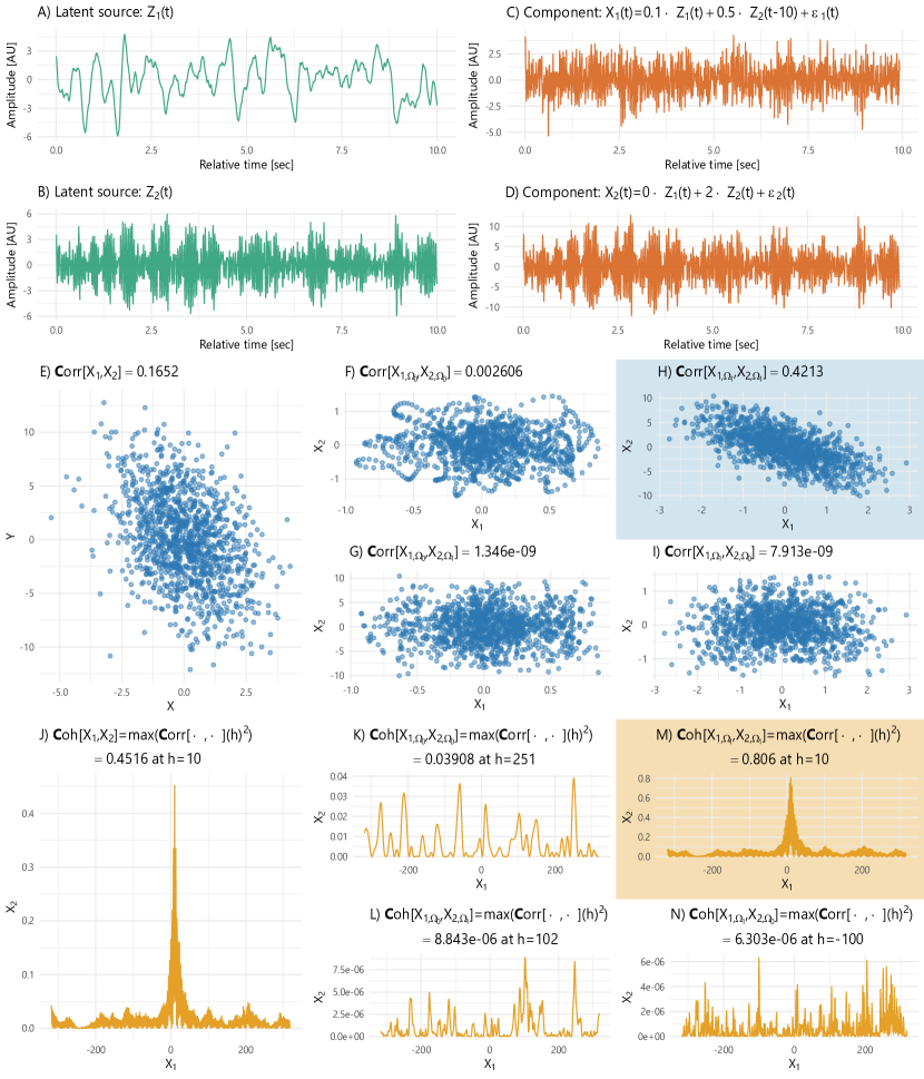
Figure 7: Simulated example 3: system with latent sources ($Z_{1}(t)$, $Z_{3}(t)$) and lagged mixed components ($X_{1}(t)$, $X_{2}(t)$). Note the high contrast between correlation and coherence in low- and high-frequency components. $\mathop{\rm{\mathbb{C}}or}\nolimits\left[X_{\Omega 0}(t),X_{\Omega 0}(t)\right]=0.0026$ and $\mathop{\rm{\mathbb{C}}or}\nolimits\left[X_{\Omega 1}(t),X_{\Omega 1}(t)\right]=0.4213$ while $\mathop{\rm{\mathbb{C}}oh}\nolimits\left\{X_{\Omega 0}(t),X_{\Omega 0}(t)\right\}=0.039$ and $\mathop{\rm{\mathbb{C}}oh}\nolimits\left\{X_{\Omega 1}(t),X_{\Omega 1}(t)\right\}=0.8060$. Furthermore, the maximum correlation in the high-frequency components is located at lag $10$.

Example 3 (Lagged mixture).

The data generating process in the previous example (Equation 2) assumes an instantaneous mixture, i.e., the observed signals at a specific time $t$, $\{X_{1}(t),X_{2}(t)\}$ depend explicitly on the latent processes $Z_{1}(t)$ and $Z_{2}(t)\}$ also at the same time $t$. However, we can extend this model towards cases when there is some lag in the mixtures, e.g., the latent source has a delayed effect on some components of the observed signals. As Nunez et al. pointed out [70], axons can have propagation speeds in the range 600-900$\frac{cm}{s}$, and considering the average distance from the cortex to the scalp is 14.70 mm for middle-aged humans [71], we presume that delays of a few milliseconds (from any neural source to the scalp) can be feasible in the EEGs. Statistically, in order to handle these lagged mixtures, we introduce the backshift operator $B^{h}$ (where $h=0,1,\ldots$) to be $B^{h}Z(t)=Z(t-h)$. Consider now the lagged mixture

$$\left(\begin{matrix}X_{1}(t)\\ X_{2}(t)\end{matrix}\right) = \left(\begin{matrix}c_{11}B^{h_{11}}&c_{12}B^{h_{12}}\\ c_{21}B^{h_{21}}&c_{22}B^{h_{22}}\end{matrix}\right)\ \ \left(\begin{matrix}Z_{1}(t)\\ Z_{2}(t)\end{matrix}\right)\ +\ \left(\begin{matrix}\epsilon_{1}(t)\\ \epsilon_{2}(t)\end{matrix}\right).$$ (10)

Here, suppose that the mixture weight $c_{21}=0$; and the lags for the latent sources are $h_{12}=0$ and $h_{22}=10$. Thus, the two observed time series are

$$X_{1}(t) = c_{11}Z_{1}(t)+c_{12}Z_{2}(t-10)+\epsilon_{2}(t)$$

$$X_{2}(t) = c_{22}Z_{2}(t)+\epsilon_{1}(t).$$

As in the previous example, the observed signals are driven by the high-frequency latent source $Z_{2}$, but the effect of $Z_{2}$ on $X_{2}$ is delayed by $10$ time units. Consider now the scatterplots of the high-frequency filtered time series at (a.) lag $0$: $X_{1,\Omega_{1}}(t)$ vs. $X_{2,\Omega_{1}}(t)$ and (b.) lag $10$: $X_{1,\Omega_{1}}(t)$ and $X_{2,\Omega_{1}}(t-10)$. In Figure 7, it is clear that the linear relationship at lag $10$ appears stronger compared to the contemporaneous correlation. Denote the cross-correlation estimate at lag $\ell$ to be

$$\widehat{r}_{12}(\Omega_{1},\ell)=\frac{\left\{\sum_{t=1}^{T}(X_{1,\Omega_{1}}(t)X_{2,\Omega_{0}}(t-\ell))\right\}^{2}}{\sum_{t=1}^{T}(X_{1,\Omega_{1}}(t))^{2}\sum_{t=1}^{T}(X_{2,\Omega_{1}}(t))^{2}\ }.$$

Then the estimated coherence at the frequency band $\Omega_{1}$ is

$$\widehat{\rho}_{12}(\Omega_{0})=\max_{\ell=0,\pm 1,\ldots}|\widehat{r}_{12}(\Omega_{1},\ell)|^{2}.$$

3.4 AR(2) processes - discretized Cramér representation

One can approximate the Cramér representation of weakly stationary processes by a representation based on latent sources with identifiable spectra where each spectrum has its own unique peak frequency and bandwidth (or spread). Here, we will consider the class of weakly stationary second-order autoregressive, or simply AR(2), models to serve as "basis" latent sources. A process $Z(t)$ is AR(2) if it admits a representation

$$Z(t)-\phi_{1}Z(t-1)-\phi_{2}Z(t-2)=W(t)$$

where $\left\{W(t)\right\}$ is white noise with ${\mathbb{E}}\left[W(t)\right]=0$ and $\mbox{Var}\left[W(t)\right]=\sigma_{W}^{2}$ and the AR(2) coefficients $\phi_{1}$ and $\phi_{2}$ must satisfy that the roots of the AR(2) polynomial function (denoted $u_{1},u_{2}$)

$$\Phi(u)=1-\phi_{1}u-\phi_{2}u^{2}$$

must satisfy $|u_{c}|>1$ for both $c=1,2$. In particular, we will consider the subclass of $AR(2)$ models whose roots are non-real complex-valued so that they are complex-conjugates of each other $u_{2}=u_{1}^{*}$ and thus they can be reparametrized as

$$u_{1}=M\exp(i2\pi\psi)\ \ {\mbox{and}}\ \ u_{2}=M\exp(-i2\pi\psi)$$

where $M>1$ and $\psi\in(-0.5,0.5)$. Note that the AR(2) model can be parametrized by the coefficients $(\phi_{1},\phi_{2})$ or by the roots $(u_{1},u_{2})$ or by the magnitude and phase of the roots $(M,\psi)$. In fact, the one-to-one relationship between the coefficients and the roots is given by

$$\phi_{1}=\frac{2}{M}\cos\left(2\pi\psi\right)\quad{\mbox{and}}\quad\phi_{2}=-\frac{1}{M^{2}}$$ (11)

One very important and interesting property of an AR(2) process with complex-valued roots is that its spectrum has a peak at $\psi$ and the spread of this peak is governed by the magnitude $M$. When the root magnitude $M\longrightarrow 1+$ then the bandwidth of the peak around $\psi$ becomes narrower. Conversely, when $M$ becomes much larger than $1$ then the bandwidth around $\psi$ becomes wider (Figure 8).

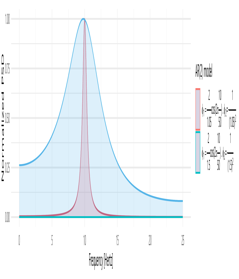
Figure 8: Autoregressive process spectrum $AR(2)$ as a function of the magnitude of its roots. The closer the magnitude is to one, the narrower the spectrum.

Example 4 (AR(2) with the peak at the alpha band).

We now describe how to specify an AR(2) process whose spectrum has a peak at $10$ Hertz. Assume that the sampling rate is $100$ Hertz with a consequent Nyquist frequency of $50$ Hertz. The roots of the AR(2) processes are then complex-valued with phase $\psi=\frac{10}{50}$ and magnitude $L$. To model an AR(2) spectra with a narrowband response around $10$ Hertz, we set the magnitude of the roots to be $L=1.05$. Moreover, to model a broadband response, we set $L=1.50$.

Therefore, the AR(2) coefficient parameters for the narrowband process are

$$\phi_{1}=\frac{2}{1.05}\cos\left(2\pi\frac{10}{50}\right)\quad{\mbox{and}}\quad\phi_{2}=-\frac{1}{(1.05)^{2}}$$ (12)

while, for the broadband signal, the AR(2) coefficients are given by

$$\phi_{1}=\frac{2}{1.50}\cos\left(2\pi\frac{10}{50}\right)\quad{\mbox{and}}\quad\phi_{2}=-\frac{1}{(1.50)^{2}}.$$ (13)

The corresponding auto-spectra of these two AR(2) processes are displayed in Figure 8.

We now construct a representation for ${\bf X}(t)$ that is a linear mixture of uncorrelated AR(2) latent processes $Z_{1},\ldots,Z_{K}$ whose spectra are identifiable with peaks within the bands $\Omega_{1}$, $\ldots,$ $\Omega_{K}$. Define $g_{k}(\omega)$ to be the spectrum of the latent AR(2) process $Z_{k}$. These spectra will be standardized so that $\int_{-0.5}^{0.5}g_{k}(\omega)d\omega=1$ for all $k=1,\ldots,K$. Moreover, these spectra have peak locations that are at unique frequencies and that these are sufficiently separated. The choice of the number of components $K$ may be guided by the standard in neuroscience where the $K=5$ bands are modeling components in the delta, theta, alpha, beta, and gamma band (as they were defined in a previous section). Another approach is developed in [72], which data-adaptively selects $K$, the peak locations, and bandwidths. Therefore, the mixture of AR(2) latent sources is given by

$$\left(\begin{matrix}X_{1}(t)\\ X_{2}(t)\\ \ldots\\ X_{P}(t)\end{matrix}\right)=\left(\begin{matrix}A_{11}&A_{12}&\ldots&A_{1K}\\ A_{21}&A_{22}&\ldots&A_{2K}\\ \ldots&{}&{}&{}\\ A_{P1}&A_{P2}&\ldots&A_{PK}\end{matrix}\right)\ \left(\begin{matrix}Z_{1}(t)\\ Z_{2}(t)\\ \ldots\\ Z_{K}(t)\end{matrix}\right)$$ (14)

.

Consider components $X_{p}$ and $X_{q}$. Suppose that, for a particular latent source $Z_{k}$, the coefficients $A_{pk}\neq 0$ and $A_{qk}\neq 0$. Then, these two signals share $Z_{k}$ as the same common component, and that $X_{p}$ and $X_{q}$ are coherent at frequency band $\Omega_{k}$.

This stochastic representation in terms of the AR(2) processes as building blocks is motivated by the result from [73] for univariate processes where the essential idea is the following: define the true spectrum of a weakly stationary process $X_{p}$ to be $f_{pp}(\omega)$ and set $f_{pp,K}^{A}(\omega)$ to be the mixture (or weighted average) of the spectrum of the $K$ AR(2) latent processes that gives the minimum discrepancy, i.e.,

$$f_{pp,K}^{A}=\mbox{inf}_{S}\int\left|f_{pp}\left(\omega\right)-S_{pp,K}^{A}\left(\omega\right)\right|\,d\omega$$ (15)

over all candidate spectra from a mixture of $K$ AR(2) processes, $S_{K}$. This discrepancy decreases as $K$ increases, and therefore, the model provides a better approximation.

3.5 Partial coherence

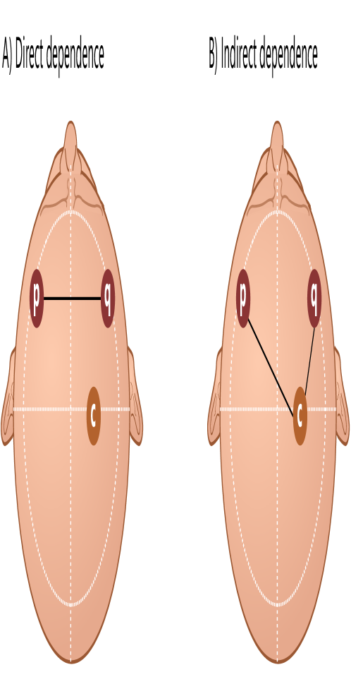
Figure 9: Direct and indirect dependence between two channels $p$ and $q$ Indirect links could appear if both channels depend on a common channel $c$.

One of the key questions of interest is determining whether the dependence between two components $X_{p}$ and $X_{q}$ is pure or it is indirect through another component $X_{c}$ (or a set of channels $c\neq p,q$). In Figure 9, we show the distinction between the pure vs. indirect dependence between $X_{p}$ and $X_{q}$. In Figure 9.B, if we remove the link between $X_{c}$ and $X_{p}$ and the link between $X_{c}$ and $X_{q}$, then there is no longer any dependence between $X_{p}$ and $X_{q}$.

A standard approach in the time domain is to calculate the partial correlation between $X_{p}$ and $X_{q}$ ([74, 75]), which is essentially the cross-correlation between them after removing the linear effect of $X_{c}$ on both $X_{p}$ and $X_{q}$. This is also achieved by taking the inverse of the covariance matrix, denoted $\Sigma^{-1}(0)$ and then standardizing this matrix by a pre- and post-multiplication of a diagonal matrix whose elements are the inverse of the square root of the diagonal elements of $\Sigma^{-1}(0)$. The procedure for the frequency domain follows in a similar manner, as outlined in Fiecas and Ombao [76]: define the inverse of the spectral matrix to be ${\bf g}(\omega)={\bf f}^{-1}(\omega)$ and let ${\bf h}(\omega)$ be a diagonal matrix whose elements are $\frac{1}{\sqrt{g_{rr}(\omega)}}$. Next, define the matrix

$$\Lambda(\omega)=-{\bf h}(\omega){\bf g}(\omega){\bf h}(\omega).$$ (16)

Then, partial coherence (PC) between components $X_{p}$ and $X_{q}$ at frequency $\omega$ is $|\Lambda_{pq}(\omega)|^{2}$.

This particular characterization of PC requires inverting the spectral matrix. This can be time computationally demanding when the dimension $P$ is large, and it also can be prone to numerical errors when the condition number of the spectral matrix ${\bf f}(\omega)$ is very high (i.e., the ratio of the largest to the smallest eigenvalue is large). This happens when there is a high degree of multicollinearity between the $\omega-$oscillations of the components of ${\bf X}$. To alleviate this problem, [77] and [76] developed a class of spectral shrinkage procedures. The procedure consists in constructing a well-conditioned estimator for the spectral matrix and hence produces a numerically stable estimate of the inverse. The starting point is to construct a "smoothed" periodogram matrix which is a nonparametric estimator of ${\bf f}(\omega)$. From a stretch of time series ${\bf X}(1),\ldots,{\bf X}(T)\}$  ($T$ even), compute the Fourier coefficients

$${\bf d}(\omega_{k})=\sum_{t=1}^{T}{\bf X}(t)\exp(-i2\pi\omega_{k}t)$$

at the fundamental frequencies $\omega_{k}=\frac{k}{T}$ where $k=-(\frac{T}{2}-1),\ldots,\frac{T}{2}).$ The $P\times P$ periodogram matrix is

$${\bf I}(\omega_{k})=\frac{1}{T}{\bf d}(\omega_{k}){\bf d}^{*}(\omega_{k})$$

where ${\bf d}^{*}$ is the complex-conjugate transpose of ${\bf d}$.

Though the periodogram matrix is asymptotically unbiased, it is not consistent. We can mitigate this issue by constructing a smoothed periodogram matrix estimator

$$\widetilde{\bf f}(\omega)=\sum_{\ell}Q_{b}(\omega_{\ell}-\omega){\bf I}(\omega_{\ell})$$

where the kernel weights $Q_{b}(u)$ are non-negative and sum to $1$. The bandwidth $b$ can be obtained using automatic bandwidth selection methods for periodogram smoothing, such as the least-squares in [78] or the gamma-deviance-GCV in [79]. The shrinkage targets are either the scaled identity matrix or a parametric matrix (that can be derived from a VAR model).

Suppose that a VAR$(L)$ model is fit to the signal ${\bf X}(t),t=1,\ldots,T\}$ $\Phi(B){\bf X}(t)={\bf W}(t)$ where ${\bf W}(t)$ is a zero-mean $P-$variate white noise with $\mathop{\rm{\mathbb{C}}ov}\nolimits{\bf W}(t)=\Sigma_{\bf W}$ and $\Phi(B)=I-\Phi_{1}B-\ldots-\Phi_{L}B^{L}$. Then the spectrum of this VAR($L$) process is

$${\bf h}(\omega)=\Phi(\exp(-i2\pi\omega))\ \Sigma_{\bf W}\ \Phi^{*}(\exp(-i2\pi\omega))$$

.

The parametric estimate of the spectral matrix, denoted ${\widetilde{\bf h}}(\omega)$, is obtained replacing $\Phi_{\ell}$, $\ell=1,\ldots,L$, by the maximum likelihood or conditional maximum likelihood estimators. The shrinkage estimator for the spectrum takes the form

$$\widehat{\bf f}(\omega)=W_{1}(\omega)\widetilde{I}(\omega)+W_{2}(\omega))\widetilde{\bf h}(\omega)$$

where the weights $W_{s}(\omega)$ fall in $(0,1)$ and $W_{1}(\omega)+W_{2}(\omega)$ for each $\omega$. Moreover, the weight for the smoothed periodogram is proportional to the mean-squared error of the parametric estimator, i.e., $W_{1}(\omega)\propto{\mathbb{E}}\lvert\widetilde{h}(\omega)\ -\ {\bf f}(\omega)|^{2}$.

This method can be interpreted as a spectrum estimator that automatically chooses the estimator with better "quality". Therefore, when the parametric estimator is "poor" (high MSE), the weights shift the estimator towards the nonparametric estimator. However, when the parametric model gives a good fit, the shrinkage shift to the parametric spectral estimate. Thus, the resulting spectral estimator has, in general, a good condition number and can be used further for the estimation of PC where the quality of the spectral information is critical.

An alternative view to the above approach in constructing partial coherence is through analyzing the oscillations. For simplicity, we consider the $\omega$-oscillations for channels $X_{p}$, $X_{q}$ and $X_{c}$, which we denote to be $X_{p,\omega}$, $X_{q,\omega}$ and $X_{c,\omega}$, respectively. At this stage, we shall consider only the contemporaneous (i.e., zero-phase or zero-lag) partial cross-correlation

$$\mathop{\rm{\mathbb{C}}or}\nolimits\{X_{p,\omega}(t),X_{q,\omega}(t)\ |\ X_{c,\omega}(t)\}.$$

To proceed, regress of $X_{p,\omega}(t)$ against $X_{c,\omega}(t)$ and extract the residuals, denoted $R_{p\dot{c},\omega}(t)$ and also $X_{q,\omega}(t)$ against $X_{c,\omega}(t)$, and extract the residuals, named as $R_{q\dot{c},\omega}(t)$.

Then, the zero-phase partial coherence between $X_{p}$ and $X_{q}$ at frequency $\omega$ is the quantity

$$\rho_{pq\dot{c}}(\omega)=\left|\mathop{\rm{\mathbb{C}}or}\nolimits\left[R_{p\dot{c},\omega},R_{q\dot{c},\omega}\right]\right|^{2}.$$

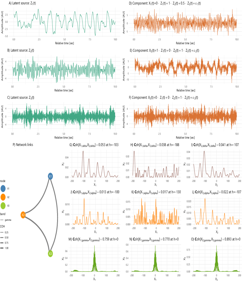
Figure 10: Coherence network of a system with a dominating gamma component (Example 5). Three latent sources (delta-, alpha- and gamma-band waves) are linearly into combined three observed components $X_{1}$, $X_{2}$ and $X_{3}$. As expected, the network map (P.) denotes that all components are related within the gamma-band. The correlation across lags is also displayed to emphasize the coherence magnitudes.

Example 5 (Partial coherence on a gamma-interacting system).

Consider the setting where the independent latent processes are specific AR(2)’s that mimic the delta, alpha, and gamma activity which we denote by $Z_{\delta}(t)$, $Z_{\alpha}(t)$ and $Z_{\gamma}(t)$. Suppose that the observed time series are $X_{1}(t)$, $X_{2}(t)$ and $X_{3}(t)$, which are defined by the mixture

$$\left(\begin{matrix}X_{1}(t)\\ X_{2}(t)\\ X_{3}(t)\end{matrix}\right) = \left(\begin{matrix}a_{1\delta}&a_{1\alpha}&a_{1\gamma}\\ a_{2\delta}&a_{2\alpha}&a_{2\gamma}\\ a_{3\delta}&a_{3\alpha}&a_{3\gamma}\end{matrix}\right)\left(\begin{matrix}Z_{\delta}(t)\\ Z_{\alpha}(t)\\ Z_{\gamma}(t)\end{matrix}\right).$$ (17)

We now examine the dependence between $X_{1}$ and $X_{2}$ under the following setting. First, suppose that $X_{3}$ contains the gamma-oscillatory activity $Z_{\gamma}$ purely, that is, $a_{3\delta}=a_{3\alpha}=0$. Next, suppose that $X_{1}$ contains only $Z_{\alpha}$ and $Z_{\gamma}$, that is, $a_{1\delta}=0$; and $X_{2}$ contains only $Z_{\delta}$ and $Z_{\gamma}$, that is, $a_{2\alpha}=0$. A realization of such a system is shown in Figure 10.

Under this construction, $X_{1}$ and $X_{2}$ have zero coherence at the $\delta$ and $\alpha$ frequency band. However, $X_{1}$ and $X_{2}$ both contain the common gamma-oscillatory activity and hence have a non-zero coherence at the gamma-band. In our particular example, $\mathop{\rm{\mathbb{C}}oh}\nolimits\left\{X_{1,\gamma},X_{2,\gamma}\right\}=0.759$, $\mathop{\rm{\mathbb{C}}oh}\nolimits\left\{X_{1,\gamma},X_{3,\gamma}\right\}=0.770$, and $\mathop{\rm{\mathbb{C}}oh}\nolimits\left\{X_{2,\gamma},X_{3,\gamma}\right\}=0.893$.

However, if we compare coherence and partial coherence (Figure 11), we can unveil some indirect dependence effects. Partial coherence between $X_{1}$ and $X_{2}$ (conditional on $X_{3}$) at the gamma-band is zero. This result indicates that if we remove $X_{3}$ (the gamma-band activity) from $X_{1}$ and $X_{2}$, then their "residuals" will no longer contain any common latent source.

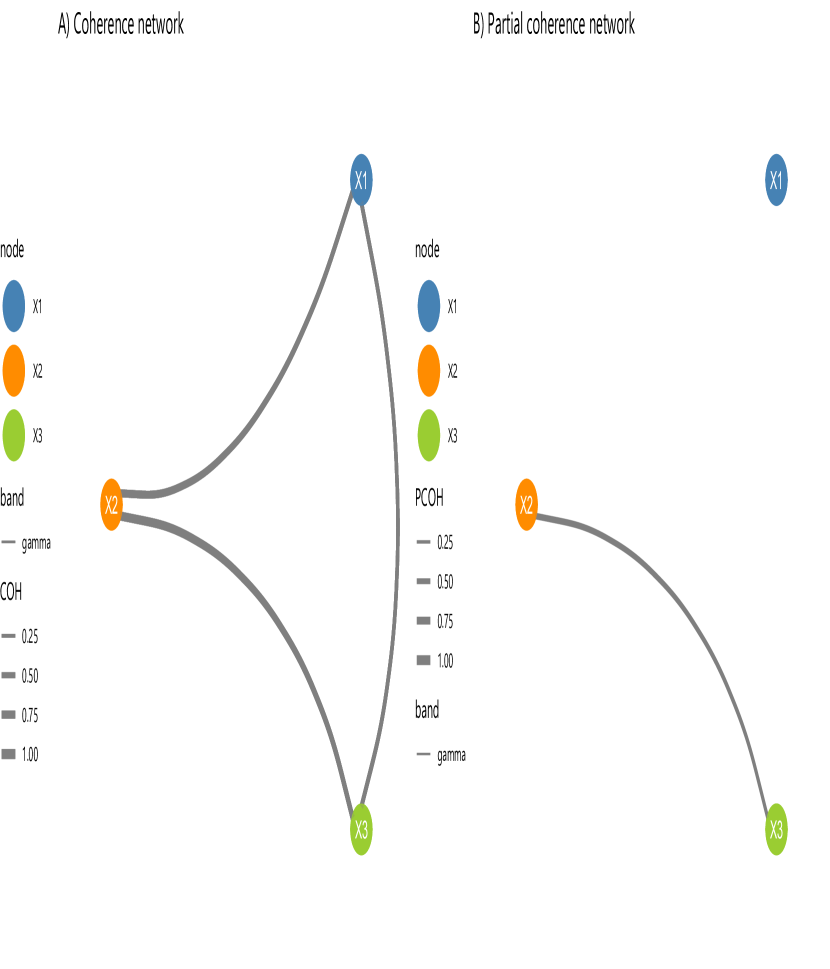
Figure 11: Comparison between coherence and partial coherence in Example 5.

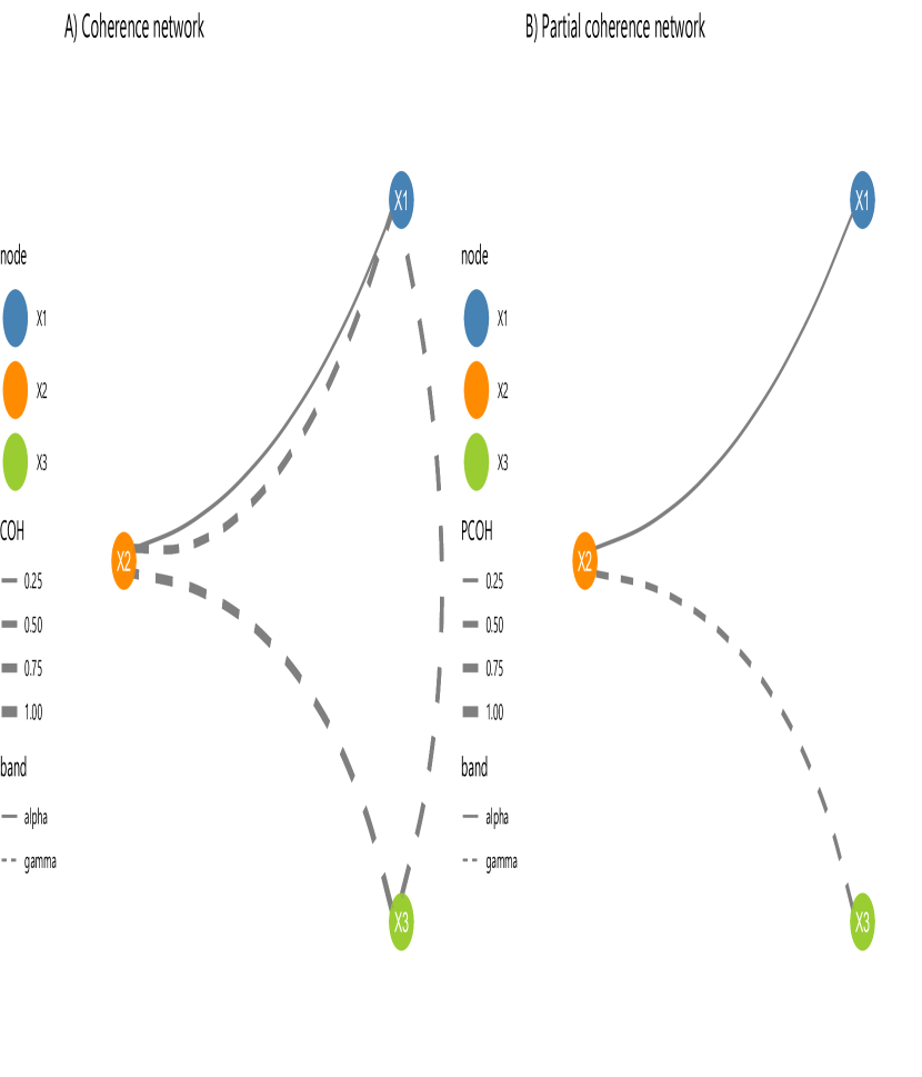
Figure 12: Comparison between coherence and partial coherence in Example 6.

Example 6 (Partial coherence).

As a continuation of Example 5, suppose that (a.) $X_{3}$ contains only gamma-oscillatory activity $Z_{\gamma}$, i.e., $a_{3\delta}=a_{3\alpha}=0$; (b.) $X_{1}$ contains only $Z_{\alpha}$ and $Z_{\gamma}$: $a_{1\delta}=0$; and (c.) $X_{2}$ contains $Z_{\delta}$, $Z_{\alpha}$ and $Z_{\gamma}$.

In such a dependence structure, we can observe the following frequency-dependent effects on $X_{1}$ and $X_{2}$:

• At the delta-band, the coherence between $X_{1}$ and $X_{2}$ is zero; and hence the partial coherence (conditioned on $X_{3}$) is also zero;

• At the alpha-band, the coherence and partial coherence between $X_{1}$ and $X_{2}$ are both non-zero;

• At the gamma band, the coherence between $X_{1}$ and $X_{2}$ is non-zero but the partial coherence is zero.

These observations can be summarized in the coherence and partial coherence networks of Figure 12.

3.6 Time-varying coherence and partial coherence

As noted, many brain signals exhibit non-stationarity. In some cases, the autospectra varies over time which indicates that the contributions of the various oscillations to the total variance change across the entire recording. In others, the autospectra might remain constant, but the strength and nature of the association between components can change. In fact, in Fiecas and Ombao [80], the coherence between a pair of tetrodes from a local field potential implanted in a monkey evolves both within a trial and even across trials in an experiment. Here, we will follow the models in [45] and in [46] to define and estimate the time-varying coherence and partial coherence.

Recall that for a weakly stationary process, we define and estimate the spectral dependence quantities through the Cramér representation

$${\bf X}(t)=\int_{-0.5}^{0.5}\exp(i2\pi\omega t)d{\bf Z}(\omega)$$

where the random increments are uncorrelated across $\omega$ and satisfy ${\mathbb{E}}d{\bf Z}(\omega)=0$, $\mbox{Var}d{\bf Z}(\omega)={\bf f}(\omega)d\omega$. An equivalent representation is

$${\bf X}(t)=\int{\bf A}(\omega)\exp(i2\pi\omega t)d{\bf U}(\omega)$$

where $d{\bf Z}(\omega)={\bf A}(\omega)d{\bf U}(\omega)$; ${\bf A}(\omega)$ is the transfer function matrix; $\mbox{Var}d{\bf U}(\omega)={\bf I}d\omega$; and the spectral matrix is

$${\bf f}(\omega)={\bf A}(\omega)\ {\bf A}^{*}(\omega).$$

The Priestley-Dahlhaus model for a locally stationary process allows the transfer function to change slowly over time. This idea was first proposed in [45], but later refined in [46] which developed an asymptotic framework for constructing a mean-squared consistent estimator for the time-varying spectral matrix. A simplified expression of the locally stationary time series model ${\bf X}(t),t=1,\ldots,T\}$ is

$${\bf X}(t)=\int_{-0.5}^{0.5}{\bf A}\left(\frac{t}{T},\omega\right)\exp\left(i2\pi\omega t\right)d{\bf U}(\omega)$$ (18)

and the time-varying spectral matrix defined on rescaled time $\nicefrac{{t}}{{T}}\in(0,1)$ and frequency $\omega\in(-0.5,0.5)$ is

$${\bf f}\left(\frac{t}{T},\omega\right)={\bf A}\left(\frac{t}{T},\omega\right)\ {\bf A}^{*}\left(\frac{t}{T},\omega\right).$$

Based on this time-varying spectral matrix, the time-varying coherence between components $X_{p}$ and $X_{q}$ at rescaled time $\nicefrac{{t}}{{T}}$ and frequency $\omega$ is

$$\rho_{pq}\left(\frac{t}{T},\omega\right)=\frac{\left|f_{pq}(\frac{t}{T},\omega)\right|^{2}}{f_{pp}\left(\frac{t}{T},\omega\right)f_{qq}\left(\frac{t}{T},\omega\right)}.$$

In a similar vein, the time-varying partial coherence between components $X_{p}$ and $X_{q}$ (conditioned on $X_{c}$) at rescaled time $\nicefrac{{t}}{{T}}$ and frequency $\omega$ is derived in a similar manner from Equation 16. The standard approach to estimating these time-varying spectral dependence measures is computing time-localized periodogram matrices and then smoothing these across frequency.

There are other models and methods for analyzing non-stationary time series. One class of methods divides the time series into quasi-stationary blocks: dyadic piecewise stationary time series models in [81]; dyadic piecewise aggregated AR(2) in [82, 83]; adaptive information-theoretic based segmentation in [84]. Another class of methods gives stochastic representations in terms of time-localized functions as building blocks like wavelets in [85]; or SLEX (smooth localized complex exponentials) in [86] and [87]. For multivariate non-stationary time series, [88] develop a procedure for selecting the best SLEX basis for signal representation. Using this basis, the estimate for the time-varying spectrum and coherence are then derived.

4 Dual-frequency dependence

In this paper, our approach to modeling dependence between the components of a multivariate time series ${\bf X}$ is through the different oscillatory activity. This was motivated by the Cramér representation ${\bf X}(t)=\int_{-0.5}^{0.5}\exp(i2\pi\omega t)d{\bf Z}(\omega)$. For Gaussian weakly stationary processes, the random increments are independent across frequencies. Hence, for $\omega\neq\omega^{\prime}$, the $\omega-$oscillations in component $X_{p}$ and the $\omega^{\prime}$-oscillations in $X_{q}$ are, by default, independent. However, there are situations when the interesting dependence structure is between different frequency oscillations.

Loéve, in [89], introduced the class of harmonizable processes, which now allow for dependence between oscillatory activities at different oscillations. Here, we shall explore different characterizations of dependence between $X_{p,\omega}(t)=\exp(i2\pi\omega t)dZ_{p}(\omega)$ and $X_{q,\omega^{\prime}}(t)=\exp(i2\pi\omega^{\prime}t)dZ_{q}(\omega^{\prime})$. The first natural measure of dependence is the linear association between these two oscillations, which we call the dual-frequency coherence

$$\rho_{(p,\omega),(q,\omega^{\prime})}=\mathop{\rm{\mathbb{C}}or}\nolimits\left[X_{p,\omega}(t),X_{q,\omega^{\prime}}(t)\right]$$

.

This opens up many possibilities of characterizations of dependence that are beyond that by classical coherence. In this paper, we will further generalize this notion of dual-frequency coherence to the situation where this measure could evolve over time. For example, during the course of one trial recording of an electroencephalogram, it is possible for coherence between the theta and gamma oscillations to be reduced immediately upon the presentation of a stimulus - but could strengthen over the course of a trial. We will summarize the notion of time-dependent dual-frequency coherence in Section 4.1. In addition, note that coherence, partial coherence, and dual-frequency coherence all capture only the linear dependence between the various oscillations. Here, we will examine other non-linear measures of dependence, such as the phase-amplitude coupling. In Section 4.2, we will illustrate how the amplitude of a gamma-oscillatory activity in channel $p$ might be change according to the phase of the alpha-activity in channel $q$. One such example could be the increase in the gamma-oscillation amplitude when the theta oscillation reaches its peak.

4.1 Evolutionary dual-frequency coherence

The modeling framework for developing the notion of a dual-frequency that evolves over time was proposed in [90] via a frequency-discretized harmonizable process which we now describe. Here, we shall focus on the practical aspect of modeling and analyzing dual-frequency coherence in the observed signals. The technical details such as the asymptotic theory required for defining the population-specific quantity are developed in [90].

Suppose that we observe the time series ${\bf X}$ and focus on a local window centered time point $t$ with $N$ observations. Define the local Fourier coefficient vector at frequency $\omega$ at time point $t$ to be

$${\bf d}(t,\omega) = \frac{1}{\sqrt{N}}\sum_{s=t-(\frac{N}{2}-1)}^{t+\frac{N}{2}}{\bf X}(s)\exp(-i2\pi\omega s)\ ,$$ (19)

and define the local dual-frequency periodogram matrix at frequencies $\omega_{j}$ and $\omega_{k}$ to be

$${\bm{I}}(t;(\omega_{j},\omega_{k}))={\bm{d}}(t,\omega_{j}){\bm{d}}(t,\omega_{k}).$$ (20)

When the data consists of several time-locked trials, one can compute trial-specific local dual-frequency periodogram matrices and then average them (across trials) in order to obtain some population-specific measure of the evolutionary dual-frequency spectral matrix. In the absence of replicated trials (i.e., the data is only from a single trial), then one can smooth the local dual-frequency periodogram matrices over time $t$ within that single trial. Denote the averaged dual-frequency periodogram matrix to be $\widehat{{\bf f}}(t,\omega_{j},\omega_{k})$. One measure of the strength of linear dependence between the $\omega_{j}$-oscillations at component $X_{p}$ and the $\omega_{k}$-oscillations at component $X_{q}$ is the time-localized dual-frequency coherence

$$\widehat{\rho}_{(p,\omega_{j}),(q,\omega_{k})}(t) =\frac{|\widehat{f}_{(p,\omega_{j}),(q,\omega_{k})}(t)|^{2}}{\widehat{f}_{(p,\omega_{j}),(p,\omega_{j})}(t)\widehat{f}_{(q,\omega_{k},(q,\omega_{k})}(t)}.$$ (21)

Consistent with the approach adopted in the paper, we investigate linear dependence between the oscillations by linear filtering. Consider two frequency bands $\Omega_{1}$ and $\Omega_{2}$ and the zero-mean filtered signals to be $X_{1,\Omega_{1}}$ and $X_{2,\Omega_{2}}$. We will provide the time-varying dual-frequency coherence estimate at a local time $t$ by first computing the local cross-covariance and local variance estimate over the window $\{t-L,\ldots,t+L\}$ (for some $L>0$) as follows

$$\widehat{f}_{(1,\Omega_{1}),(2,\Omega_{2})}(t) =\frac{1}{N}\sum_{s=t-(\frac{N}{2}-1)}^{t+\frac{N}{2}}X_{1,\omega_{1}}(s)X_{2,\omega_{2}}(s)$$

$$\widehat{f}_{(1,\Omega_{1}),(1,\Omega_{1})}(t) =\frac{1}{N}\sum_{s=t-(\frac{N}{2}-1)}^{t+\frac{N}{2}}X_{1,\omega_{1}}(s)X_{1,\omega_{1}}(s)$$

$$\widehat{f}_{(2,\Omega_{2}),(2,\Omega_{2})}(t) =\frac{1}{N}\sum_{s=t-(\frac{N}{2}-1)}^{t+\frac{N}{2}}X_{2,\omega_{2}}(s)X_{2,\omega_{2}}(s).$$

The estimated local dual-frequency coherence at local time $t$ is

$$\widehat{\rho}_{(1,\Omega_{1}),(2,\Omega_{2})}(t)=\frac{|\widehat{f}_{(1,\Omega_{1}),(2,\Omega_{2})}(t)|^{2}}{\widehat{f}_{(1,\Omega_{1}),(1,\Omega_{1})}(t)\widehat{f}_{(2,\Omega_{2}),(2,\Omega_{2}}(t)}$$ (22)

4.2 Phase-Amplitude coupling

In the previous sections, we examined coherence and partial coherence - both of which aim to measure the strength of linear dependence between a pair of channels or components $X_{p}$ and $X_{q}$ through the oscillatory activity at the same frequency. In Section 4, we examine dependence at different frequencies and how this dependence may change over time through the evolutionary dual-frequency coherence. However, all of these only examine linear dependence. In the neuroscience literature, it was acknowledged that inter-frequency modulation could also appear as a different category of dependence in the brain networks. Similarly to coherence, this dependence type implies interactions within the frequency domain: spectral components in $\Omega_{H}$ are modulated by components resonating at frequencies in $\Omega_{L}$. When the modulator $\Omega_{H}$ works at a high frequency, and the modulated signal $\Omega_{L}$, this type of dependence is named phase-amplitude coupling (PAC). Baseline PAC networks in the human brain changes since birth [91], and specific delta-theta PAC patterns can be altered due to anesthetic effects [92].

A common method to quantify PAC in time series was introduced by Tort et al. [93] through the modulation index (MI) for univariate signals. We should emphasize that this metric is not the same as the homonym "modulation index" defined for amplitude-modulated systems [94, p. 591]. To estimate MI, let $x_{\Omega}$ be a filtered time series with its spectrum concentrated only in the interval $\Omega$. Then, its analytic signal $y_{\Omega}$ will be defined via the Hilbert transform:

$$y_{\Omega}\left(t\right)=x_{\Omega}\left(t\right)+j\left(\frac{1}{\pi t}\ast x_{\Omega}\left(t\right)\right),$$

The analytic $y_{\Omega}(t)$ can be expressed using an exponential form,

$$y_{\Omega}\left(t\right)=A_{\Omega}\left(t\right)\exp\left(j\phi_{\Omega}\left(t\right)\right).$$

such that the instantaneous phase and amplitude are identified through $\phi_{\Omega}(t)$ and $A_{\Omega}(t)$, respectively.

Now obtain $y_{\Omega_{L}}(t)$ and $y_{\Omega_{H}}(t)$ for a target low-frequency range $\Omega_{L}$ and a high-frequency interval $\Omega_{H}$ such as delta and gamma, respectively. Now, consider the joint signals $T=\bigl{(}A_{\Omega_{L}},\phi_{\Omega_{H}}\bigr{)}$. The original algorithm, described by Tort et al., suggests creating a partition of the phase domain $Q$: $Q=\cup_{j=1}^{N}Q_{j}\quad Q_{j}=\left[2\pi\frac{j-1}{N}2\pi\frac{j}{N}\right)$ and estimate the marginal mean value in each partition

$$P(j)=\mathbb{E}\left(T\mid\phi_{\Omega_{H}}=\phi\right)\quad\phi\in Q_{j}$$

Under the non-modulation hypothesis, $P(j)$ should resemble a uniform distribution $P_{U}(j)=1\,\forall j$. MI is then introduced as a normalized measure of the divergence between of the difference between $P(j)$ and the uniform alternative $P_{U}(j)$:

$$\text{MI}=\frac{1}{\log\left(N\right)}D_{KL}\left(P,U\right)$$

where $D_{KL}(\cdot)$ is the Kullback-Leibler divergence:

$$D_{KL}\left(P,Q\right)=\sum_{k=1}^{N}P\left(k\right)\log\left(\frac{P\left(i\right)}{Q\left(i\right)}\right)$$

Note that in those cases where no specific frequency band is known, we suggest starting exploring PAC phenomena in the data using the "smoothed" signals (low-frequency) and their residuals (high-frequency components). We refer to [95, 96, 97] for a comprehensive description of time-memory efficient estimation methods.

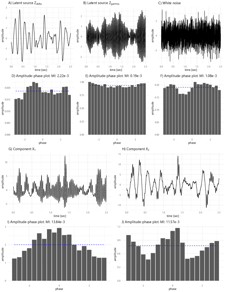
Figure 13: Phase-amplitude coupling in Example 7: phase-amplitude graphs $P(j)$ and modulation indexes (MIs) for the latent sources $Z_{\delta}(t)$, $Z_{\gamma}(t)$ and the observations $X_{1}(t)$ and $X_{2}(t)$. Note that MI values in $X_{1}(t)$ and $X_{2}(t)$ are up to five times greater than MI magnitudes of the latent sources or the noise $\varepsilon(t)$.

Example 7 (Phase-amplitude coupling).

Define the theta-band and gamma-band latent sources to be $Z_{\theta}$ and $Z_{\gamma}$, respectively. Let assume that some modulation effects are observed as a result of non-linear mixtures of the latent sources:

$$\left(\begin{matrix}X_{1}(t)\\ X_{2}(t)\end{matrix}\right) =\left(\begin{matrix}A_{1,\delta}(t)&A_{1,\gamma}(t)\\ A_{2,\delta}(t)&A_{2,\gamma}(t)\end{matrix}\right)\left(\begin{matrix}Z_{\theta}(t)\\ Z_{\gamma}(t)\end{matrix}\right)+\varepsilon\bigr{(}t\bigl{)}$$

where $\varepsilon\bigr{(}t\bigl{)}\sim\mathcal{N}\bigr{(}0,\Sigma_{\varepsilon}\bigl{)}$ with a covariance matrix $\Sigma_{\varepsilon}=0.1{\bf I}$ such that ${\bf I}$ is an identity matrix.

Let us assume that two phase-amplitude coupling effects are observed:

• $X_{1}(t)$ denotes an amplitude-modulation effect where the amplitude of $Z_{\theta}(t)$ instantaneously leads to the amplitude’s changes in the $\gamma$-oscillations. Therefore, the mixture functions are defined as $A_{1,\delta}\left(t\right)=Z_{\gamma}\left(t\right)+1$ and $A_{1,\gamma}\left(t\right)=2$.

• $X_{2}(t)$ shows a modulation effect where the $Z_{\gamma}(t)$ component has a low impact on the $\delta$-oscillations: $A_{2,\delta}\left(t\right)=4$ and $A_{2,\gamma}\left(t\right)=Z_{\theta}$.

Figure 13 shows a simulation of this process along with the modulation indexes for $Z_{\delta}(t)$, $Z_{\gamma}(t)$, $\varepsilon(t)$ and the observed components $X_{1}(t)$ and $X_{2}(t)$. It is visually apparent that $P(j)$ is closer to $P_{U}(j)$ in scenarios without modulation effects (Figure 13.A-F). In addition, we can remark that the modulated process $X_{2}(t)$ implies an alteration on the extreme values of the process, and it could also be modeled using statistical models for extreme values [38].

5 Partial directed coherence and spectral causality

All previously mentioned spectral measures of dependence: coherence, partial coherence, dual-frequency coherence, and evolutionary dual-frequency coherence all ignore the lead-lag dependence between oscillatory components. This notion of lead-lag is very important in neuroscience, particularly in identifying effective connectivity between brain regions or channels. In fact, many pioneering models for brain connectivity were applied to functional magnetic resonance imaging data and therefore took into account the spatial structure in the brain data ([98]). To address the computational issues for spatial covariance [99] introduced a scalable multi-scale approach (local for voxels within a region of interest; global for regions of interest in the entire network). In another approach, [100] the temporal covariance structure is diagonalized (and hence sparsified) by applying a Fourier transform on the voxel-specific time series while taking into account variation across subjects through a mixed-effects modeling framework. In a recent work, [101] developed a method for mediation analysis in fMRI data, and [102] proposed a variational Bayes algorithm with reduced computational costs.

There have also been a number of statistical methods for modeling dynamic connectivity in fMRI: dynamic correlation in [103]; switching vector autoregressive (VAR) model in [104], regime-switching factor models in [105] and [106]; Bayesian model of brain networks in [102, 107, 108, 109, 110, 107]; models for high dimensional networks in [111]; detection of dynamic community structure in [112], [113] and [114]. In [115], a Bayesian VAR model was used to assess stroke-induced changes in the functional connectivity structure.

In this section, we will cover approaches to identify lead-lag structures in brain signals using the vector autoregressive (VAR) models. Modeling these lead-lag dynamics is crucial to understanding the nature of brain systems, the impact of shocking events (such as stroke) on the dynamic configuration of such systems, and the downstream effect of such disruption on cognition and behavior. However, the emphasis of this section will be on investigating frequency-band specific lead-lag dynamics. Thus, while the classical VAR model characterizes the effect of the past observation of the signal $X_{q}$ on a future observation on the signal $X_{q}$, our emphasis here will be on modeling and assessing the impact of the previous oscillatory activity $X_{q,\omega_{1}}$ on the future oscillations $X_{p,\omega_{2}}$.

5.1 Vector autoregressive (VAR) models

A $P$-variate time series ${\bf X}$ is said to be a vector autoregressive process of order $L$ (denoted VAR$(L)$) if it is weakly stationary and can be expressed as $\Phi(B){\bf X}(t)={\bf W}(t)$ where $\bigl{\{}{\bf W}(t)\bigr{\}}$ is white noise with ${\mathbb{E}}\left[{\bf W}(t)\right]=0$ for all time $t$ and $\mathop{\rm{\mathbb{C}}ov}\nolimits\left[{\bf W}(t)\right]=\Sigma_{\bf W}$ and

$$\Phi(B)=I-\Phi_{1}B-\Phi_{2}B^{2}-\ldots-\Phi_{L}B^{L}$$

and $\Phi_{\ell}$, $\ell=1,\ldots,L$ are the $P\times P$ VAR coefficient matrices. A comprehensive exposition of VAR models, including conditions for causality and methods for estimation of the coefficient matrices $\{\Phi_{\ell}\}$, are provided in [116]. Note that from classical time series literature, the notion of "causality" is different from that of Granger causality. A time series ${\bf X}$ is causal if ${\bf X}(t)$ depends only on the current or past white noise $\{{\bf W}(s),\ s=t,t-1,t-2,\ldots\}$.

Consider the two components $X_{p}$ and $X_{q}$. From the point of view of forecasting, we say that “$X_{q}$ Granger-causes $X_{p}$" (we write $X_{q}\longrightarrow X_{p}$) if the squared error for the forecast of $X_{p}$ that uses the past values of $X_{q}$ is lower than that for the forecast that does not use the past values of $X_{q}$. Under the context of VAR models, note that

$$X_{p}(t)=\sum_{\ell=1}^{L}\Phi_{pq,\ell}X_{q}(t-\ell)+\sum_{r\neq q}\sum_{\ell=1}^{L}\Phi_{pr,\ell}X_{r}(t-\ell)$$ (23)

where $\Phi_{pq,\ell}$ is the $(p,q)$ element of the matrix $\Phi_{\ell}$. For $X_{p}(t)$, it is the coefficient associated with the past value $X_{q}(t-\ell)$. Thus, $X_{q}\longrightarrow X_{p}$) if there exists some lag $\ell*$ where $\Phi_{pq,\ell*}\neq 0$. There is a large body of work on causality, starting with the seminal paper by [117]. This was further studied in [118], [119], [120]. Additional applications for subject- and group-level analysis was also analyzed in [121]. Recently, under non-stationarity, the nature of Granger-causality could evolve over time and this was investigated in [122]. Despite the fact that the concept of causality are derived from the spectral representation, the focus on the interpretations for causality has not been on the actual oscillatory activities. The goal is this section is to refocus the spotlight on this very important role of the oscillations in determining causality and, in general, directionality between a pair of signals.

5.2 Partial directed coherence

As noted, all previously discussed measures of coherence lack the important information on directionality. The concept of partial directed coherence (PDC), introduced in [123] and [124], gives this additional information. Define the VAR(L) transfer function to be

$$\Phi(\omega)=I-\sum_{\ell=1}^{P}\Phi_{\ell}\exp(-i2\pi\omega\ell)$$

and denote $\Phi_{pq}(\omega)$ to be the $(p,q)$ element of the transfer function matrix $\Phi(\omega)$. Then the PDC, from component $X_{q}$ to $X_{p}$, at frequency $\omega$ is

$$\pi_{pq}(\omega)=\frac{|\Phi_{pq}(\omega)|^{2}}{\sum_{rq}|\Phi_{rq}(\omega)|^{2}}.$$

Note that $\pi_{pq}(\omega)$ lies in $[0,1]$ and measures the amount of information flow, at frequency $\omega$, from component $X_{q}$ to $X_{p}$, relative to the total amount of information flow from $X_{q}$ to all components. When $\pi_{pq}(\omega)$ is close to $1$ then most of the $\omega$-information flow from $X_{q}$ goes directly to component $X_{p}$. Under this framework, we estimate PDC fitting a VAR model to the data ${\bf X}(t),t=1,\ldots,T\}$ where the optimal order $L$ can be selected using some objective criterion like the Akaike information criterion (AIC) or the Bayesian-Schwartz information criterion (BIC).

Example 8 (Connectivity network comparison).

Assume a system with four channels that can be described by the following sparse VAR$(2)$ model:

$$\left(\begin{matrix}X_{1}(t)\\ X_{2}(t)\\ X_{3}(t)\\ X_{4}(t)\end{matrix}\right) =\left(\begin{matrix}\phi_{\beta,1}&\frac{1}{2}&0&0\\ 0&0&1&0\\ 0&0&\phi_{\delta,1}&0\\ 0&0&0&\phi_{\gamma,1}\end{matrix}\right)\left(\begin{matrix}X_{1}(t-1)\\ X_{2}(t-1)\\ X_{3}(t-1)\\ X_{4}(t-1)\end{matrix}\right)+\left(\begin{matrix}\phi_{\beta,2}&0&0&0\\ 0&0&0&1\\ 0&0&\phi_{\delta,2}&0\\ 0&0&0&\phi_{\gamma,2}\end{matrix}\right)\left(\begin{matrix}X_{1}(t-2)\\ X_{2}(t-2)\\ X_{3}(t-2)\\ X_{4}(t-2)\end{matrix}\right)+\varepsilon\left(t\right)$$

where $\left(\phi_{\delta,1},\phi_{\delta,2}\right)$, $\left(\phi_{\gamma,1},\phi_{\gamma,2}\right)$ and $\left(\phi_{\beta,1},\phi_{\beta,2}\right)$ were calculated as described in Equation 11 with $M=1.049787$ and $\psi_{\delta}=\frac{2}{128}$, $\psi_{\gamma}=\frac{40}{128}$ and $\psi_{\beta}=\frac{20}{128}$, respectively. The noise $\varepsilon\left(t\right)\sim\mathcal{N}\left(0,\Sigma\right)$ where $\Sigma$ is a diagonal matrix. Consequently, $X_{3}(t)$ and $X_{4}(t)$ are independent delta and gamma components.

In this multivariate system, direct and indirect lagged dependence links are denoted: $X_{3}$ and $X_{4}$ directly lead $X_{2}$: $X_{4}(t-2)\Longrightarrow X_{2}(t)$, $X_{3}(t-1)\Longrightarrow X_{2}(t)$, while both indirectly affect $X_{1}$ through $X_{2}$: $X_{2}(t-1)\Longrightarrow X_{1}(t)$. Previously, coherence (COH) and partial coherence (PCOH) were applied to identify instantaneous direct dependencies. Figure 14 and Table 1 show the connectivity networks that can be estimated using PDC in addition to both dependence metrics along with their magnitudes.

We should emphasize that VAR mismodeling can considerably affect the dependence metrics that rely on them (as can be observed in Figure 14.F). However, these effects can be mitigated with regularization techniques that are discussed in Section 6.3. For a comprehensive empirical analysis of the mismodeling phenomena in connectivity, we refer to [125].

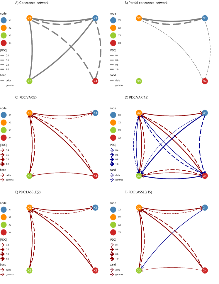
Figure 14: Connectivity networks for the system in Example 8. Dependence metrics were obtained from six methods: coherence (COH), partial coherence (PCOH), partial directed coherence (PDC) estimated with an OLS-estimated VAR(2) and VAR(15) models, and PDC estimated with a regularized second- and fifteenth-order LASSLE models.

Band	Link	COH	PCOH	PDC: VAR(2)	PDC: VAR(15)	PDC: LASSLE(2)	PDC: LASSLE(15)
$\delta$	$X_{2}\Rightarrow X_{1}$	0.9996	0.9749	0.5096	0.5334	0.5097	0.5097
0-4	$X_{1}\Rightarrow X_{2}$			0.0000	0.0070	0.0000	0.0000
Hertz	$X_{3}\Rightarrow X_{1}$	0.9959	0.2074	0.0001	0.0438	0.0000	0.0000
	$X_{1}\Rightarrow X_{3}$			0.1754	0.6465	0.1878	0.4634
	$X_{4}\Rightarrow X_{1}$	0.0257	0.0347	0.0001	0.0440	0.0000	0.0000
	$X_{1}\Rightarrow X_{4}$			0.0061	0.3040	0.0115	0.0031
	$X_{3}\Rightarrow X_{2}$	0.9961	0.3320	0.5774	0.5786	0.5774	0.5773
	$X_{2}\Rightarrow X_{3}$			0.2799	0.4561	0.0900	0.1495
	$X_{4}\Rightarrow X_{2}$	0.0259	0.0336	0.5773	0.5789	0.5773	0.5773
	$X_{2}\Rightarrow X_{4}$			0.0061	0.4376	0.0041	0.0096
	$X_{4}\Rightarrow X_{3}$	0.0239	0.2715	0.4152	0.4152	0.0448	0.3549
	$X_{3}\Rightarrow X_{4}$			0.0052	0.6050	0.0000	0.0000
	$X_{2}\Rightarrow X_{1}$	0.9857	0.9863	0.3854	0.2901	0.3854	0.3855
	$X_{1}\Rightarrow X_{2}$			0.0000	0.0547	0.0000	0.0000
$\gamma$	$X_{3}\Rightarrow X_{1}$	0.0280	0.0404	0.0001	0.1165	0.0000	0.0000
30-50	$X_{1}\Rightarrow X_{3}$			0.0009	0.3611	0.0009	0.0036
Hertz	$X_{4}\Rightarrow X_{1}$	0.9860	0.3938	0.0000	0.1170	0.0000	0.0000
	$X_{1}\Rightarrow X_{4}$			0.1233	0.6449	0.0599	0.0882
	$X_{3}\Rightarrow X_{2}$	0.0232	0.0394	0.5773	0.5800	0.5774	0.5773
	$X_{2}\Rightarrow X_{3}$			0.0012	0.4270	0.0006	0.0023
	$X_{4}\Rightarrow X_{2}$	0.9996	0.3967	0.5774	0.5808	0.5773	0.5773
	$X_{2}\Rightarrow X_{4}$			0.0212	0.5365	0.0216	0.0323
	$X_{4}\Rightarrow X_{3}$	0.0236	0.0179	0.0017	0.5550	0.0003	0.0025
	$X_{3}\Rightarrow X_{4}$			0.2119	0.3476	0.0000	0.0000

Table 1: Comparison of the connectivity metrics between channels and frequency in Example 8: coherence (COH), partial coherence (PCOH), and partial directed coherence (PDC). PDC was estimated through four different vector autoregressive models: VAR(2) and VAR(15) and regularized models: LASSLE(2) and LASSLE(15).

5.3 Time-varying PDC

A natural question to ask would be how to characterize and estimate PDC when it is changing over time. As noted, during the course of a trial, an experiment or even within an epoch, the brain functional network is dynamic ([114]). Thus, one may characterize a time-varying PDC through a time-varying VAR model

$$\Phi_{t}(B)=I-I-\Phi_{t,1}B-\Phi_{t,2}B^{2}-\ldots-\Phi_{t,L}B^{L}$$

where $\Phi_{t,\ell}$ is the VAR coefficient matrix for lag $\ell$ at time $t$. The dimensionality of the parameters for at any time $t$ for a time-varying VAR$(L)$ model is $P^{2}L$. Thus, in order to have a sufficient number of observations at any time $t$, one can estimate the time-varying coefficient matrices $\{\Phi_{t,\ell},\ell=1,\ldots,L\}$ by fitting a local conditional least squares estimate to a local data at time $\{t-\left(\frac{N}{2}-1\right)$, $\ldots,\frac{N}{2}\}$. In addition to borrowing information from observations within a window (to increase the number of observations), it is also advisable to apply some regularization which will be discussed in Section 6.3. After obtaining estimates $\{\widehat{\Phi}_{t,\ell}\}$, we compute the estimate of the time-varying transfer function $\widehat{\Phi}(t,\omega)$, which then leads to a time-varying PDC estimate

$$\pi_{pq}(t,\omega)=\frac{|\Phi_{pq}(t,\omega)|^{2}}{\sum_{rq}|\Phi_{rq}(t,\omega)|^{2}}.$$

PDC has provided the important frequency-specific information of directionality from one component to another - which is already beyond what coherence, partial coherence, and dual-frequency coherence can offer. One can compare the PDC from $X_{q}$ to $X_{p}$ of the alpha-band vs. the gamma-band since this relative strength is a directed flow of communication that can vary across frequency oscillations.

5.4 Spectral causality

There are limitations with PDC as a measure of dependence. First, it does not indicate the phase or the physical time lag between oscillations. While it is useful to know the direction $X_{q}$ $\Longrightarrow$ $X_{p}$ at frequency $\omega$, it would be crucial to identify the time lag $\tau_{pq,\omega}$ via some relationship such as

$$X_{p,\omega}(t)=A_{pq,\omega}X_{q,\omega}(t-\tau_{pq,\omega})+\epsilon_{p,\omega}(t)$$

for some coefficient $A_{pq,\omega}$ and time lag $\tau_{pq,\omega}$ that could vary depending on the channels and also on the frequency (or frequency bands). Second, PDC only captures directionality only for the same frequency (or frequency bands). It only models how the past of $\omega$-oscillation in channel $X_{q}$ could impact the future $\omega$-oscillation in channel $X_{p}$. It would be more desirable to capture between-frequencies directionality (as in the dual-frequency setting), for example,

$$X_{p,\omega_{1}}(t)=A_{pq,\omega_{1}}X_{a,\omega_{1}}(t-\tau_{pq,\omega_{1}})+A_{pq,\omega_{2}}X_{a,\omega_{2}}(t-\tau_{pq,\omega_{2}})+\epsilon_{p,\omega_{1}}(t)$$

The third limitation is that it captures only the linear associations between the oscillations. We overcome the first and second limitations through the spectral vector autoregressive (Spectral-VAR) model. This current form of the model is linear and non-linear variants that are based on biophysical models will be reported in the future. An initial estimation approach is introduced in [126].

Consider the situation where we want to investigate the potential causality from channel $X_{q}$ to the gamma-oscillation of channel $X_{p}$. As used in previous examples, we will denote the delta, theta, alpha, beta, and gamma oscillations of $X_{q}$ to be, respectively,

$$X_{q,\delta},X_{q,\theta},X_{q,\alpha},X_{q,\beta}\ {\mbox{and}}\ X_{q,\gamma}.$$

The oscillations for channel $X_{p}$ are denoted in a similar manner. The key distinction here is that these oscillations are obtained from a one-sided filter

$$X_{q,\delta}(t)=\sum_{j=0}^{\infty}C_{\delta,j}X_{q}(t-j)$$

in order to properly capture these lead-lag relationships.

Example 9 (Two-sided filter lead-lag distortion).

Let $Z_{\delta}(t)$, $Z_{\beta}(t)$ and $Z_{\gamma}(t)$ be three latent oscillatory signals with main frequencies at 2, 15 and 30 Hertz, respectively. Now assume that two signals are observed:

$$\left(\begin{matrix}X_{1}(t)\\ X_{2}(t)\end{matrix}\right) =\left(\begin{matrix}Z_{\delta}(t)\\ Z_{\delta}(t-10)&+Z_{\beta}(t-10)&+Z_{\gamma}(t-10)\end{matrix}\right)+\frac{1}{2}\left(\begin{matrix}\varepsilon_{1}(t)\\ \varepsilon_{2}(t)\end{matrix}\right)$$

where $\varepsilon_{1}(t)$ and $\varepsilon_{2}(t)$ are uncorrelated white noise with unit variance.

Assume an one- and two-sided FIR(100) filter and denote their output filtered signals as $X_{k,delta}^{(1-sided)}$ and $X_{k,delta}^{(2-sided)}$ for a given channel $X_{k}$. Even though that coherence between the delta-filtered $X_{1}(t)$ and $X_{2}(t)$ maintains a reasonable similar magnitude, it can be observed that the lead-lag relationship is not kept (Figure 15.C-D)

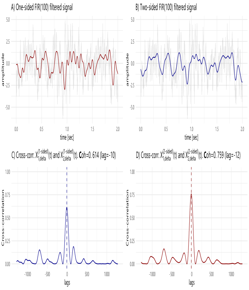
Figure 15: Effects of an one-sided and two-sided filter in the lead-lag relationship (Example 9).

The spectral-VAR model of order $L$ for predicting the gamma-oscillation of $X_{p}$ is defined to be

$$X_{p,\gamma}(t) =\sum_{\ell=1}^{L}\left\{A_{(p,\gamma),(p,\delta),\ell}X_{p,\delta}(t-\ell)+A_{(p,\gamma),(q,\delta)}X_{q,\delta}(t-\ell)\right\}$$

$$+\ldots$$

$$+\sum_{\ell=1}^{L}\left\{A_{(p,\gamma),(p,\gamma),\ell}X_{p,\gamma}(t-\ell)+A_{(p,\gamma),(q,\gamma)}X_{q,\gamma}(t-\ell)+\epsilon_{p,\gamma}(t)\right\}.$$

Under this set-up, we say that there is a Granger-causality relation from the past alpha-oscillatory activity in $X_{q}$ to the future gamma-oscillation in $X_{p}$ if there exists a time lag $\ell*$ such that $A_{(p,\gamma),(q,\alpha),\ell*}\neq 0$.

As a final remark, the usual VAR model does not address the need for frequency-specific lead-lag (or Granger-causality) relationships. Suppose that, from the usual VAR model, we conclude that $X_{q}\Longrightarrow$ $X_{p}$. This information is “coarse" in the sense that it lacks the information on the specific frequency band (or bands) in $X_{q}$ that Granger-cause the specific band(s) in the $X_{p}$ as well as the precise channel-specific and frequency bands-specific time-lag between these oscillations.

6 High-Dimensional Signals

Most brain signals are high-dimensional in space and time. For example, fMRI data are typically recorded over $10^{5}$ brain voxels and across hundreds of time points sampled at a speed of one-complete image every 2 seconds (the sampling rate is $0.50$ Hertz). Therefore, fMRI data are highly dense in space (though they have poor temporal resolution). In contrast, EEG data are more sparse in space as the number of channels can vary from about 20 to 256, depending on the adopted recording system. However, the range of the number of temporal observations can be in the millions (with sampling frequency typically ranging from $100-1000$ Hertz). In this section, we will present two approaches to dealing with high-dimensional signals: (a.) by creating low-dimensional signal summaries such as principal component analysis; and (b.) by including a penalization component in estimation.

6.1 Spectral principal components analysis

It is common for components of a $P$-variate signal $X$ to display some multi-collinearity, especially between biomedical signals recorded as spatially close locations. It is therefore natural to obtain a low-dimensional summary that captures the main characteristics of these signals. One way is through the classical principal component analysis (PCA) – or linear auto-encoder/decoder in machine learning jargon – which is described as follows.

The auto-encoder algorithm described in [127] is a general approach to learning compressed (low-dimensional) representations of the input data, which in this particular scenario are high-dimensional brain signals. The algorithm consists of two parts, namely, the (a.) encoder and (b.) decoder. The encoder function $F:{\bf X}\rightarrow{\bf Y}$ is a mapping from the original high-dimensional space ${\bf X}$ to lower dimension space ${\bf Y}$. Due to its dimensionality reduction purpose, $F$ is also called compression step. The decoder or reconstruction function, defined as $D:{\bf F}\rightarrow{\bf X}$ is a mapping from the encoded (low-dimensional) space to the original high-dimensional space. Consider a time series $\{{\bf X}(t),t=1,\ldots,T\}$ generated by some process $p({\bf X})$. The optimal mapping encoder $F$ and decoder $D$ minimize the expected reconstruction error defined as

$$L\left(F,D\right)={\mathbb{E}}_{p({\bf X})}\left\|{\bf X}-D(F({\bf X}))\right\|^{2}_{F}$$ (24)

where $\left\|\cdot\right\|_{F}$ is the Frobenius norm, which is defined as $\left\||E\right\||_{F}=\sqrt{\text{Trace}(EE^{\prime})}$.

Here, we will consider only the special cases where both the encoder and decoder are linear transformations of the original signal, which can be either instantaneous mixing or filtering. For these types of functions, the solution is closely related to principal component analysis (PCA) defined under the aforementioned Frobenius norm based on the squared error of reconstruction.

Let us consider the first family of encoder-decoders: instantaneous mixture processes of the observed signal $\{{\bf X}(t),\ t=1,\ldots,T\}$. Under this model, the compressed signal is obtained as ${\bf Y}(t)={\bf A}^{\prime}{\bf X}(t)$. Denote the dimension of ${\bf Y}(t)$ to be $Q$; the dimension of ${\bf X}(t)$ to be $P$ and $Q<P$. Similarly, the signal is reconstructed by the decoder $\widehat{\bf X}(t)={\bf B}{\bf Y}(t)$. For identifiability purposes, ${A}^{\prime}{A}=I_{Q}$, and $\mathop{\rm{\mathbb{C}}ov}\nolimits{\bf Y}(t)$ is diagonal so that the components of the compressed signal X are uncorrelated. The optimal low-dimensional representation maximizes the best reconstruction accuracy (or minimizes the squared error loss) via the following steps:

• Obtain the eigenvalues-eigenvectors of the covariance matrix of ${\bf X}$: $\Sigma^{\bf X}(0)$. Denote e-value and e-vector pair as $\{(\lambda_{p},{\bf v}_{p})\}_{p=1}^{P}$ where $\lambda_{1}>\ldots,>\lambda_{P}$ and $\|{\bf v}_{p}\|=1$ for all $p$. When $\Sigma^{\bf X}(0)$ is not known, we obtain an estimator from the observed signal $\{{\bf X}(t),\ t=1,\ldots,T\}$.

• The solution for the optimal encoder-decoder is derived as

  $$\widehat{{A}}^{\prime}=\widehat{{B}}=[{\bf v}_{1},\ldots,{\bf v}_{Q}]\ \ \ {\mbox{and}}\ \ \ \widehat{\bf Y}(t)=\widehat{{A}}{\bf X}(t)\ .$$

Under the squared reconstruction error as the loss function, the solution is identical to applying PCA on the input signals using the covariance matrix at lag zero. Indeed, the solution accounts for most of the variation of the time series (or gives the minimum squared reconstruction error), among all instantaneous linear projections with the same dimension.

When the goal is to obtain summaries from time series data, it is important for the encoded (compressed) and decoded (expanded) components to capture the entire temporal dynamics (lead-lag structure) of the signal. The previous approach is a contemporaneous mixture and thus could miss important dynamics in the data. The second category of linear encoder-decoders relies on the idea of applying linear filters on $\{{\bf X}(t)\}$ instead of applying a merely instantaneous mixture. In contrast to the contemporaneous mixture, this encoder is more flexible and its lower-dimensional representation is written as

$${\bf Y}(t)=\sum_{\ell=\infty}^{\infty}A^{\prime}(\ell){\bf X}(t-\ell)$$ (25)

where $A^{\prime}(\ell)\in\mathbb{C}^{Q\times P}$ with $Q<P$. The components of the summarized signal, ${Y}_{p}(t)$ and ${Y}_{q}(t)$, have zero coherency. That is, the components $Y_{p}(t)$ and $Y_{q}(s)$ are uncorrelated at all time points $t$ and $s$, and hence also for all lags. The reconstruction (decoder) function has the following form

$$\widehat{\bf X}(t)=\sum_{\ell=-\infty}^{\infty}B(\ell){\bf Y}(t-\ell)$$ (26)

where $B(\ell)\in\mathbb{C}^{P\times Q}$ is the transformation coefficient matrix.

The optimal values of $A(\ell)$ and $B(\ell)$ are chosen to minimize the reconstruction error defined in Equation 24. The solution is obtained via principal components analysis of the spectral matrix ${\bf f}(\omega)$ of the process ${\bf X}$ – rather than the lag-0 covariance matrix. Denote the eigenvalues of the spectral matrix at frequency $\omega$ to be $\{\lambda_{1}(\omega)>\lambda_{2}(\omega),\dots,\lambda_{P}(\omega)\}$, and the corresponding eigenvectors to be $\{{\bf v}_{1}(\omega),{\bf v}_{2}(\omega),\dots,{\bf v}_{n}(\omega)\}$. Then, the solution is

$${A}(\ell) = \int_{-1/2}^{1/2}{A}(\omega)\exp(i2\pi\ell\omega)d\omega$$ (27)

$${B}(\ell) = \int_{-1/2}^{1/2}{B}(\omega)\exp(i2\pi\ell\omega)d\omega$$ (28)

where ${B}(\omega)={A}^{*}(\omega)$ and ${A}(\omega)=[{\bf v}_{1}(\omega),\dots,{\bf v}_{Q}(\omega)]$.

This dimension reduction procedure was originally described in [128], and in this paper, we shall refer to this as the “Spectral-PCA" method (SPCA). This method was extended to various nonstationary settings, including [129], where the stochastic representation of a multichannel signal was selected from a library of orthogonal localized Fourier waveforms (SLEX). In [130], the time-varying spectral PCA was developed under the context of the Priestley-Dahlhaus model, which was further refined in [131] for the experimental setting where there are replicated multivariate nonstationary signals. In practical data analysis, the interest is on the magnitude of the components of the eigenvector (or eigenvectors) with the largest eigenvalues because they represent the loading or weights given by the components of the observed signal. We motivate this in the example below.

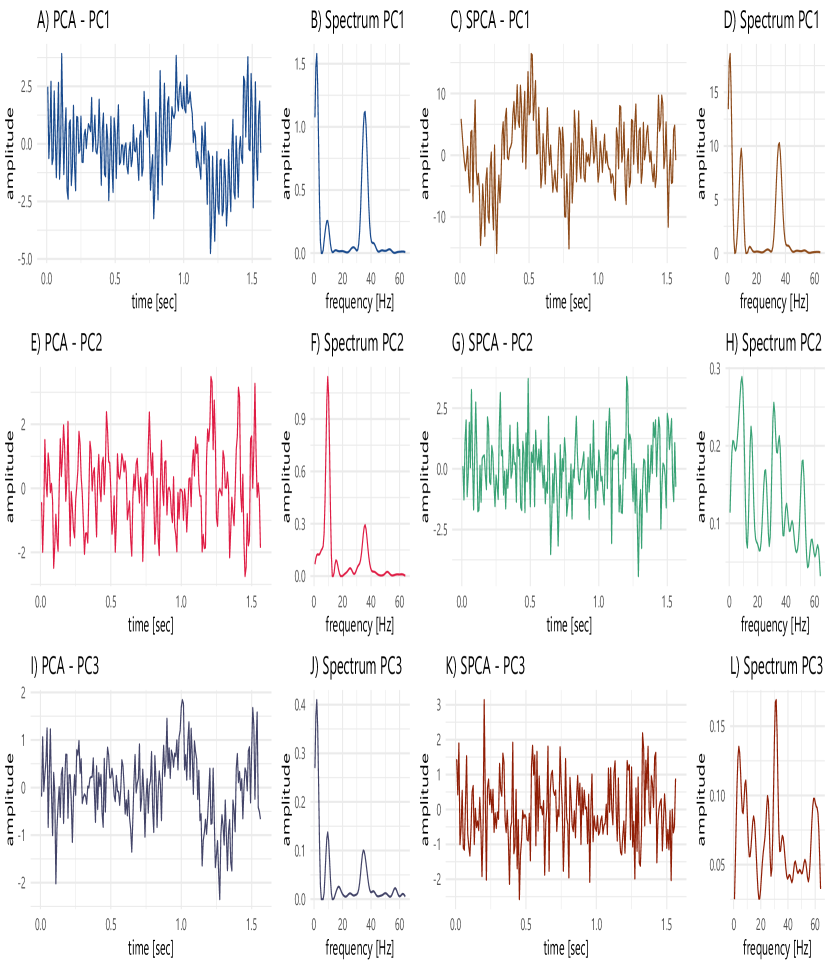
Figure 16: Summary signals ${\bf Y}(t)$ using PCA and SPCA (Example 10). The components in the time and frequency domain are shown for both encoding algorithms.

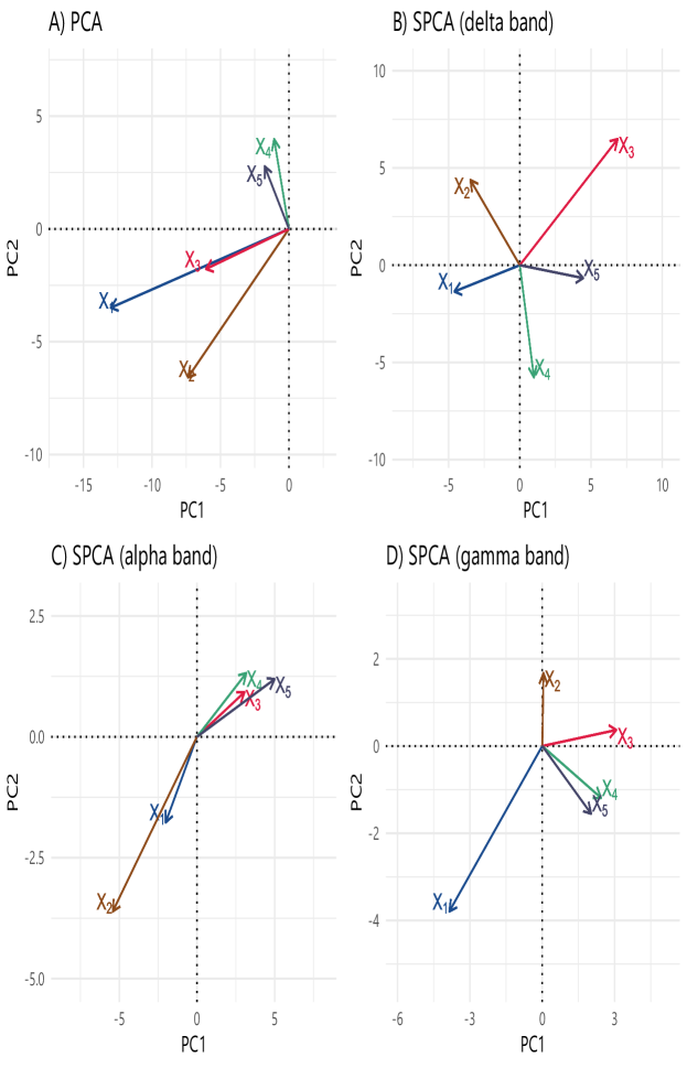
Figure 17: Two-dimensional loadings of Example 10: PCA loadings ($\widehat{A}$) and mean SPCA loadings ($A(\omega)$) in the frequency bands: delta (0-4 Hertz), alpha (8-12 Hertz), and gamma (30-45 Hertz).

Example 10 (Example on spectral PCA).

Suppose that we have latent sources that are oscillations at the delta, alpha, and gamma bands, denoted by $Z_{\delta}$, $Z_{\alpha}$ and $Z_{\gamma}$, respectively. The observed signal is a mixture ${\bf X}(t)$ of the latent sources

$$\left(\begin{matrix}X_{1}(t)\\ X_{2}(t)\\ X_{3}(t)\\ X_{4}(t)\\ X_{5}(t)\end{matrix}\right) = \left(\begin{matrix}1&0&1\\ 0&0&1\\ 1&0&1\\ 0&1&0\\ 1&1&0\end{matrix}\right)\left(\begin{matrix}Z_{\delta}(t)\\ Z_{\alpha}(t)\\ Z_{\gamma}(t)\end{matrix}\right)\ +\ \left(\begin{matrix}\epsilon_{1}(t)\\ \epsilon_{2}(t)\\ \epsilon_{3}(t)\\ \epsilon_{4}(t)\\ \epsilon_{5}(t)\end{matrix}\right)$$ (29)

The first two compressed components of the instantaneous mixture (PCA) and the spectral PCA (SPCA) are shown in Figure 16. Note that all three first PCA principal components capture a mixture of the latent sources, and therefore, contain the delta, alpha, and gamma oscillations in different proportions. This oscillation mixture is made evident from its loadings (Figure 17.A) where $X_{1},\ldots,X_{6}$. Nevertheless, the first component emphasizes the delta and gamma sources, whereas the second component highlights the alpha and gamma bands.

On the other hand, the first SPCA component captures all the main spectral information of the latent oscillations (Figure 16.D). Due to the properties of SPCA, mean loadings can be evaluated as a function of the frequency, and the contribution of the components can be evaluated for each frequency band (through the loadings in Figure 17.B-D). For instance, consider the encoding processes on the alpha band: the main descriptive components are $X_{4}$ and $X_{5}$, but SPCA compensates the effects of the other signals in such a way that the sum of $X_{1}$ and $X_{2}$ (delta and gamma) will mitigate the effect of $X_{3}$ (also delta and gamma).

6.2 Brain Connectivity Analysis through Low-Dimensional Embedding

As noted, neuronal populations behave in a coordinated manner both during resting-state and while executing tasks such as learning and memory retention. One of the major challenges to modeling connectivity in brain signals is the high dimensionality. In the case of fMRI data with $V=10^{5}$ voxels, one would need to compute connectivity from in the order of $10^{10}$ pairs of voxels (or $V(V-1)/2$ pairs). To alleviate this problem, one approach in fMRI is to parcellate the entire brain volume into distinct regions of interest (ROIs) and hence connectivity is computed between ROIs rather than between voxels. This approach effectively reduces the dimensionality since connectivity is computed between broad regions rather than at the voxel level. This is also justified by the fact that neighboring voxels tend to behave similarly and thus it would be redundant to calculate connectivity between all pairs of voxels. Motivated by the ROI-based approach in fMRI, one procedure to study connectivity in EEG signals is to first create groups of channels using some anatomical information. Depending on the parcellation of the brain cortex, a cortical region could correspond to 15-25 EEG channels [132]. Within each group, we compute the signal summaries using spectral principal components analysis. In the second step, we model connectivity between groups of channels by computing dependence between the summaries. More precisely, suppose that the $P$-dimensional time series ${\bf X}$ is segmented into $R$ groups denoted by ${\bf X}_{r}$, $r=1,\ldots,R$. In each group ${\bf X}_{r}$, summaries are computed, which we denote by ${\bf Y}_{r}$. Thus, connectivity between groups $r$ and $r^{\prime}$ will be derived from the summaries ${\bf Y}_{r}$ and ${\bf Y}_{r^{\prime}}$

There are many possible methods for computing summaries. When biomedical signals can be modeled as functional data, principal components analysis (PCA) extensions have been formulated, as it is shown in [133]. Under sampled time series, a naïve solution is to compute the average across all channels within a group. In fact, connectivity analyses of functional magnetic resonance imaging (fMRI) are usually conducted by taking the time series averaged across voxels in pre-defined ROIs ([134, 135]). However, simple averaging is problematic, especially when some of the signals are out of phase often observed in EEGs due to averaging can lead to signal cancellation. Sato et al. [136] already pointed the pitfalls and suggests a data-driven approach via conventional PCA, which essentially provides an instantaneous (or contemporaneous) mixing of time series. Other approaches for modeling brain connectivity from high-dimensional brain imaging data include Dynamic Connectivity Regression (DCR) [137], Dynamic Conditional Correlation (DCC) [138], group independent component analysis (ICA) [139, 140], and sparse vector autoregressive (VAR) modeling [141]. Here, we propose extract summaries ${\bf Y}_{r}$ from each group of channels via the spectral PCA method in Equations 25 and 26 above.

6.3 Regularized vector autoregressive models

Recall that connectivity measures such as coherence, partial coherence and partial directed coherence are based on the frequency domain but they can be motivated under the context of parametric models. In fact, PDC was developed within the framework of a vector autoregressive (VAR) model. Here, we discuss the challenges of fitting a VAR model when the number of channels $P$ and the VAR order $D$ are large. In this setting there will be $P^{2}D$ number of VAR parameters that have to be estimated. The goal here is to introduce some of the regularization procedures.

The classic method for estimating the VAR parameters is via the least squares estimator (or conditional likelihood for Gaussian signals), which is generally unbiased. However, the least-squares estimators (LSE) are problematic because of the high computational demand and that it does not possess specificity for coefficients whose true values are zero. In many applications, brain networks are high-dimensional structures that are assumed to be sparse but interconnected. To address the problem of high dimensional parameter space, a common estimation approach is by penalized regression ([142], [143], [144], [145]), and a specific method is the LASSO (least absolute shrinkage and selection operator). Compared to the LSE approach, the LASSO has a lower computational cost ([146]) and has higher specificity of zero-coefficients. However, the main limitation of the LASSO (and, in general, most regularization methods) is the bias of the non-zero coefficients’ estimators. Thus, it could lead to misleading results when investigating the true strength of brain connectivity. By leveraging the strengths of each of the LSE and the LASSO, Hu et al. [147] proposes a (hybrid) two-step estimation procedure: the LASSLE method. This approach suggest a two-phase estimation process. In the first stage, the LASSO is applied to identify coefficients whose estimates are set to 0. In the second stage, the coefficients that survived the thresholding from the first stage are re-estimated via LSE. LASSLE was shown to have inherent low-bias for non-zero estimates, high specificity for zero-estimates, and significantly lower mean squared error (MSE) in the simulation study.

An example of the impact of using regularized models in connectivity estimation was visually shown in Figure 14.E-F (from Example 8).

7 Modeling dependence in non-stationary brain signals

Contrary to common intuition, the brain operates actively even during resting periods, and therefore this is also reflected in the brain signal dynamics [148]. Brain signals from various modalities, such as magnetoencephalograms, electroencephalograms, local field potentials, near-infrared optical signals, and functional magnetic resonance imaging, all show statistical properties that evolve over time during rest and various task-related settings (memory, somatosensory, audio-visual). Such time-evolving characteristics are also observed across species: laboratory rats, macaque monkeys, and humans. These changes are seen in the variance, auto-correlation, cross-correlation, coherence, partial coherence, partial directed coherence, or graph-network properties [149]. It is worth noting that in some experimental settings, changes in the cross-channel dependence may be more pronounced than changes within a channel (e.g., auto-spectrum and variance). This phenomenon was observed in [80], where changes in cross-coherence were observed in a macaque monkey local field potentials and correlated with the learning task.

In this section, an overview of the different approaches to analyzing non-stationary signals will be discussed. The first class of approaches gives stochastic representations using the Fourier waveforms or some multi-scale orthonormal basis such as wavelets, wavelet packets, and the smoothed localized complex exponentials (SLEX). In the second class of methods, the signals are segmented into quasi-stationary blocks, and the time-varying spectral properties such as the auto-spectra, coherence, and partial coherence are computed within each time block. This class of approaches produces a specific tiling of the time-frequency plane. The third class of approaches assumes that the dynamic brain activity fluctuates or switches between a finite number of "states". Each of these states, defined by a vector autoregressive model or a stochastic block model, gives a unique characterization of the brain functional network. This class of models depicts brain responses to a stimulus (or background activity during resting state) as switching between these states.

7.1 Stochastic representations

Priestley-Dahlhaus model. The major theme in this paper is the characterization of brain signals as mixtures of randomly oscillating waveforms. So far, the emphasis has been on stochastic representations in terms of the Fourier waveforms. As already noted, the Cramér representation of a $P$-dimensional stationary time series ${\bf X}_{t}$

$${\bf X}(t)=\int_{-0.50}^{0.50}{\bf A}(\omega)\exp(i2\pi\omega t)d{\bf Z}(\omega)$$

where ${\bf A}(\omega)$ is a $P\times P$ the transfer function matrix and $\{d{\bf Z}(\omega)\}$ is a random increment process with ${\mathbb{E}}d{\bf Z}(\omega)=0$ and $\mathop{\rm{\mathbb{C}}ov}\nolimits[d{\bf Z}(\omega),d{\bf Z}(\omega^{\prime})]={\bf I}\delta(\omega-\omega)$ where $\delta$ is the Dirac-delta function. To illustrate the role of the transfer function, define $A_{pq}(\omega)$ to be the $(p,q)$ element of ${\bf A}(\omega)$;  and  $dZ_{p}(\omega)$ to be the $p$-th element of the random vector $d{\bf Z}(\omega)$. The spectral matrix is ${\bf f}(\omega)={\bf A}(\omega){\bf A}*(\omega)$.

The time series at channels $p$ and $q$ can be written as

$$X_{p}(t) =\sum_{r=1}^{P}\int_{-0.50}^{0.50}A_{pr}(\omega)\exp(i2\pi\omega t)dZ_{r}(\omega)$$

$$X_{q}(t) =\sum_{r=1}^{P}\int_{-0.50}^{0.50}A_{qr}(\omega)\exp(i2\pi\omega t)dZ_{r}(\omega).$$

They are coherent at frequency $\omega$ if there exists some $r$ where $A_{pr}(\omega)\neq 0$ and $A_{qr}(\omega)\neq 0$. In this case, ${\bf A}_{p}(\omega){\bf A}_{q}^{*}(\omega)\neq 0$  (where ${\bf A}_{r}(\omega)$ is the $r$-th row of the transfer function matrix ${\bf A}(\omega)$.

Under stationarity, spectral cross-dependence between signals (e.g., coherence) is constant over time. For brain signals, dependence between channels varies across time. A time-dependent generalization of the Cramér representation is the Priestly-Dahlhaus model ([45] and [150]). For a time series of length $T$, the Dahlhaus-Priestley model uses a time-dependent transfer function where

$${\bf X}(t)=\int_{-0.50}^{0.50}{\bf A}(\frac{t}{T},\omega)\exp(i2\pi\omega t)d{\bf Z}(\omega).$$

where the transfer function ${\bf A}(\frac{t}{T},\omega)$ is defined on rescaled time $\frac{t}{T}$  $\in(0,1)$ and frequency $\omega\in(-0.50,0.50)$. Under this model, the mixture changes over time because the random coefficient vector ${\bf A}(\frac{t}{T},\omega)\ d{\bf Z}(\omega)$ also changes with time. The time-varying spectrum is ${\bf f}(u,\omega)={\bf A}(u,\omega){\bf A}*(u,\omega)$ and, consequently, the time-varying coherence between channels $p$ and $q$ is

$$\rho_{pq}(u,\omega)=\frac{|f_{pq}(u,\omega)|^{2}}{f_{pp}(u,\omega)f_{qq}(u,\omega)}.$$

To estimate the time-varying spectrum at a particular rescaled time $u\in(0,1)$, local observations around this time point are used to form local periodograms, which are then smoothed over frequency. Alternatively, one can fit a localized semi-parametric estimator as shown in [76]. Note that a change-point detection extension was introduced in [151].

Locally stationary wavelet process. An alternative to the Priestley-Dahlhaus model is the locally stationary wavelet process (LSW) proposed in [85], which uses the wavelets as building blocks. Under the LSW model, a scale- and time-dependent wavelet spectrum is defined. The original LSW model is univariate and has been extended to the multivariate setting in [152] as follows. A time series ${\bf X}(t),t=1,2,\ldots,T$ is a multivariate LSW process if it has the representation

$${\bf X}(t)=\sum_{j}\sum_{k}{\bf V}_{j}(\frac{k}{T})\psi_{j,t-k}{\bf Z}_{jk}$$

where $\{\psi_{j,t-k}\}$ is a set of discrete non-decimated wavelets; ${\bf V}_{j}(\frac{k}{T})$ is the transfer function matrix which is lower-triangular; and ${\bf Z}_{jk}$ are uncorrelated zero mean with covariance matrix equals to the identity matrix. Note that ${\bf Z}_{jk}$ in the multivariate LSW is the analog of $d{\bf Z}(\omega)$ in the Fourier-based stochastic representation. The classification procedure for the LSW model was developed in [153] for univariate time series and in [154] for multivariate time series. Given training data (signals with known group membership), these methods extract the wavelet scale-shift features or projections that separate the different classes of signals. These features are then used to classify a test signal. These wavelet-based classification methods are demonstrated to be asymptotically consistent, i.e., the probability of misclassification decreases to zero as the length of the test signal increases.

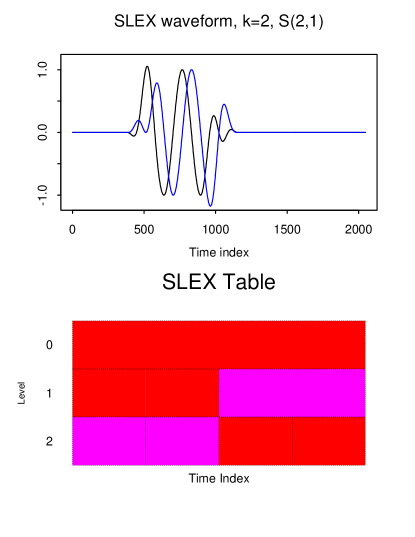
Figure 18: Top: SLEX waveform (real and imaginary parts) with local support at dyadic block $B(2,1)$. Bottom: SLEX library with level $J=2$. The SLEX library consists of a finite number of bases and each basis gives a dyadic segmentation of the time axis. The set of magenta-colored blocks represent one particular basis with time blocks $B(2,0)B(2,1),B(1,1)$ which corresponds to the segmentation on rescaled time: $\bigl{[}0,\frac{1}{4}\bigr{)}\cup bigl[\frac{1}{4},\frac{1}{2}\bigr{)}\cup\bigl{[}\frac{1}{2},1\bigr{]}$.

Figure 19: Spectral estimation of a linearly frequency evolving signal using four representation methods: short-time Fourier transform, wavelet transform, SLEX and DASAR.

Figure 20: Time-frequence representation of 32-second EEG recordings from channels on the frontal left (F3) and right (F4) hemisphere using short-time Fourier transform, wavelet transform, SLEX and DASAR.

The SLEX model. There are other time-localized bases that are well suited for representing non-stationary time series. In particular, the SLEX (smooth localized complex exponentials) waveforms are ideal for a comprehensive analysis that is a time-dependent generalization of Fourier-based methods. The SLEX waveforms are time-localized versions of the Fourier waveforms and they are constructed by applying a projection operator ([88]). The starting point is to build the SLEX library which is a collection of many bases. These bases consist of functions defined on a dyadic support on rescaled time. In Figure 18, see the plot of a specific SLEX waveform with support on the second quarter of the rescaled time and with approximately 2 complete cycles within that block. In this example, a tree is grown to level $J=2$ (i.e., the finest blocks have support with width $\frac{1}{2^{2}}$). There are 5 bases in this library and each basis corresponds to a specific dyadic segmentation of $[0,1]$. One particular basis is represented by the magenta-colored blocks which are denoted by $B(2,0),B(2,1),B(1,1)$. This basis also corresponds to the specific segmentation $[0,\frac{1}{4})\cup[\frac{1}{4},\frac{1}{2})\cup[\frac{1}{2},1]$. Define $\mathcal{B}$ to be a set of indices $(j,b)$ that make up one particular basis. In this particular example, $\mathcal{B}=\{(2,0),(2,1),(1,1)\}$. Denote an SLEX waveform with support on block $B(j,b)$ oscillating at frequency $\omega$ is denoted as $\Psi_{j,b,\omega}(t)$. Then the SLEX model corresponding to this particular basis $\mathcal{B}$ is

$${\bf X}(t)=\sum_{(j,b)\in\mathcal{B}}\int_{-0.50}^{0.50}\Theta_{j,b}(\omega)\psi_{j,b,\omega}(t)d{\bf Z}_{j,b}(\omega)$$ (30)

where $\Theta_{j,b}(\omega)$ is the SLEX transfer function defined on time block $B(j,b)$ and $\{d{\bf Z}_{j,b}(\omega)\}$ is an increment random process that is orthonormal across time blocks $(j,b)$ and frequencies $\omega$. For a given SLEX basis, the time-dependent SLEX spectral matrix is

$${\bf f}_{s}(t/T,\omega)=\Theta_{j,b}(\omega)\Theta_{j,b}^{*}(\omega)$$

for $t$ in the time block $B(j,b)$. Thus, the SLEX auto-spectra and the SLEX-coherence are defined in a similar way as the classical Fourier approach.

The main advantage of the SLEX methods for analyzing non-stationary signals is the flexibility offered by the library of bases. Depending on the particular problem of interest, a "best" basis is selected from this collection of bases. Each SLEX basis gives rise to a unique segmentation and an SLEX model. In [86], a penalized Kullback-Leibler criterion was proposed for selecting the SLEX basis. This criterion jointly minimizes: (i.) the error of discrepancy between the empirical time-varying SLEX spectrum and the candidate true SLEX spectrum, and (ii.) the complexity as measured by the number of blocks for each candidate basis. For the problem of modeling high dimensional time series, [88] develop a procedure for model selection and dimension reduction through the SLEX principal components analysis. In some applications, the goal is to discriminate between classes of signals and to classify the test signal. Under the SLEX framework, there is a rich set of time-frequency features derived from the many potential bases. The SLEX method for discrimination selects the basis that gives the maximal discrepancy between classes of signals (e.g., signals from healthy controls vs. disease groups). A classification procedure for univariate signals was proposed in [155] and for multivariate signals in [156]. The SLEX method for classification is also demonstrated to be consistent, i.e., the probability of misclassification converges to zero as the length of the test signal increases.

7.2 Change-points approach

One broad class of methods for analyzing non-stationary signals identifies the change-points and thus segments the signals into quasi-stationary time blocks. There are many of these change-points methods and a few most relevant to brain signal analysis are discussed here.

One line of segmentation methods is based on dyadic segmentation. In [81], a dyadic segmentation of a non-stationary univariate signal is developed. The signal is split dyadically up to some specified level $J$ so that at each level $j$ there are exactly $2^{j}$. Each block at level $j$ (mother block) is split into two blocks (children blocks). Starting from the deepest level of the tree, the spectra at the adjoining children blocks are estimated and then compared. When they are similar (based on some discrepancy metric), then these children blocks are combined to form one mother block. Otherwise, they are kept as distinct blocks. A large discrepancy between the spectral estimates indicates that there is a change-point. The Adak method also imposes a penalty for complexity in order to prevent a stationary block from unnecessarily splitting into two. The SLEX methods in [88] and [86] can also be viewed as dyadic segmentation methods even though the segmentation is merely a by-product of the best model (or best SLEX basis) selected from the penalized Kullback-Leibler criterion. Another method based on a similar dyadic division is presented in [157] and [158]: the dyadic aggregated autoregressive model (DASAR). In this representation, where each dyadic block at level $j$ is modeled using an aggregated autoregressive model (with degrees of freedom in the number of maximum components and the maximum order of each autoregressive component). Rules for its tree expansion are similar to the abovementioned for SLEX. By construction, DASAR blocks represents one resonating component through two parameters: central frequency and bandwidth (exponential of the negative root modulus $M$ in Equation 11). This compact representation shows notable relevance for classification purposes [157] and frequency tracking [158].

For completeness, we also enumerate the other interesting change-point methods that have been either applied to brain signals or are potentially useful in analyzing brain signals: binary segmentation for transformed autoregressive conditionally heteroscedastic models in [159]; group lasso in [160]; score-type test statistics for VAR-based models in [161]; test of non-stationarity based on the discrete Fourier transform in [162].

Example 11 (Non-stationary signal with linearly frequency evolution).

Let us assume a non-stationary time series $x(t)$ that has a continuous evolving frequency, i.e. a chirp signal, with a frequency starting at $\omega_{0}$ and incrementing $\Delta\omega$ Hertz each second:

$$x(t)=2\sin\bigr{(}2\pi\bigr{(}\omega_{0}+\Delta\omega t\bigl{)}t\bigl{)}+\varepsilon(t)$$

where $\varepsilon(t)\sim\mathcal{N}(0,1)$ is unit-variance white noise. Recall that these types of signals have been observed in seismic events [163, p.10-11], and also during epileptic episodes as Schiff et al. observed [164].

Figure 19 shows the spectral estimations obtained through short-time Fourier transform, wavelet transform, SLEX and DASAR. Note that the four of them were capable of detecting the time-evolving resonator.

Example 12 (Time-frequency EEG representation).

Recall the ADHD-EEG dataset described in Section 2. In Figure 20, we show the time-varying spectral response of the signals at channel F3 and F4 in the frequency interval 10–30 Hertz (beta band). Remark that the power at the 10-Hertz and 20-Hertz components are changing over time: 20-Hertz oscillations appear stronger at 8-12 seconds and 16-21 seconds with higher magnitudes in the left hemisphere.

7.3 Switching Processes and Community Detection

Another class of models characterizes changes in brain connectivity networks via a Markov-switching between states. Many approaches that use the sliding window or fit some time-varying coefficient models have difficulty in capturing abrupt changes. A Markov-switching dynamic factor model was proposed in [165] which captures dynamic connectivity states multivariate brain signals driven by lower-dimensional latent factors. A regime-switching vector autoregressive (SVAR) factor process was used to measure the dynamic directed connectivity. There is also an emerging line of models for brain connectivity that are based on stochastic block models. Indeed there is accumulating evidence that suggests that functional connectivity patterns are dynamically evolving over multiple time scales during rest and while performing a cognitive task. However, functional connectivity tends to be temporally clustered into a finite number of connectivity states. These are distinct connectivity patterns that recur over the course of the experiment. Recent work in [114] characterizes dynamic functional connectivity - specifically the state-driven changes in community organization of brain networks. A key contribution is that the approach takes into account variation across individuals. Many key innovations are being developed in this line of modeling, and they are anticipated to set the trend given the ability of these methods to handle high dimensionality datasets while providing results that are easily interpretable.

7.4 Time-varying dependence between filtered signals

Previously described methods for analyzing frequency-specific dependence between channels $X_{p}(t)$ and $X_{q}(t)$ can be extended to the non-stationary setting where this dependence can evolve over time. Recall that $X_{p,\omega}(t)$ and $X_{q,\omega}(t)$ are the $\omega$-oscillations derived from the two channels. Thus, the time-varying correlation between these oscillations is defined to be

$$\rho_{pq,\omega}(t^{*})=\mathop{\rm{\mathbb{C}}or}\nolimits\left(X_{p,\omega}(t^{*}),X_{q,\omega}(t^{*})\right).$$

The natural approach for estimating $\rho_{pq,\omega}(t^{*})$ is to form a sliding window and then compute the local correlation within each window. This approach is motivated by a time-dependent generalization of the mixture model in Equations 2, 3 and LABEL:Eq:MultiAR2Mixture,

$$\left(\begin{matrix}X_{1}(t)\\ X_{2}(t)\\ \ldots\\ X_{P}(t)\end{matrix}\right)=\left(\begin{matrix}A_{11}(t)&A_{12}(t)&\ldots&A_{1K}(t)\\ A_{21}(t)&A_{22}(t)&\ldots&A_{2K}(t)\\ \ldots&{}&{}&{}\\ A_{P1}(t)&A_{P2}(t)&\ldots&A_{PK}(t)\end{matrix}\right)\ \left(\begin{matrix}Z_{1}(t)\\ Z_{2}(t)\\ \ldots\\ Z_{K}(t)\end{matrix}\right).$$ (31)

The above model specifies the mixture matrix to have components $A_{pq}(t)$ that change with time. The time-varying mixture model in Equation 7.4 can be further generalized by allowing for temporal delay $A_{pq}(t)B^{d_{pq}}$, which will be captured by the backshift operator $B^{d_{pq}}$.

8 Code availability and data reproducibility

An R package (ECOSTASpecDepRef) was developed to provide a reference implementation for the algorithms discussed in the current paper, as well as the procedures for replicating the results shown in Examples 1–10. The source code is available at the repository https://github.com/biostatistics-kaust/ecosta-spectral-dependence.

9 Conclusion

This paper presents a general approach to modeling dependence in multivariate signals through the oscillatory activities extracted from each channel. The unifying theme is to explore the strength of dependence and possible lead-lag dynamics through filtering. The proposed framework is sufficiently comprehensive given its capability to model and study both linear and non-linear dependence in both contemporaneous and lagged configurations. Furthermore, it was demonstrated here that some of the most prominent frequency domain measures such as coherence, partial coherence, and dual-frequency coherence could be derived as special cases under this general framework.

There are numerous open problems in analyzing time series from designed experiments, with the spectral dependence approach, that were not addressed in this paper due to space constraints. Among them, we can mention the following possible experimental scenarios: (i.) There could be well-defined labeled groups, with their own dependence characteristics, according to disease (controls vs. ADHD), stimulus types (reading vs. math), cognitive load (easy vs. difficult). (ii.) There could be several participants within each group, and consequently, the models should account for the cross-subject variation of the brain’s functional response within groups. (iii.) There could be repeated expositions (or trials) to the same stimulus, and the model should be able to extract the common information across responses while simultaneously modeling trial-wise variations of brain response. (iv.) There could be different temporal scales in the experiment, and the model should take into account transient responses (i.e., within a trial or epoch), long-term responses (across the trials in an experiment) while considering the developmental changes in the human brain on longitudinal scales.

Statistical models should also allow for assessing differences in the fixed effects (e.g., control vs. disease) while also accounting for between-subject variation. A candidate approach can be performed via mixed-effects models, such as the framework proposed in [166] and [121], or fully Bayesian approaches, as the methods proposed in [115] and [167]. In addition to the need for formal statistical models, there is also a need to develop new approaches for studying possible non-linear dependence through high-dimensional models. These methods should leverage advances in dimensionality reduction, statistical/machine learning, and optimization in order to examine these complex dependence structures from high-dimensional models.

References

- Sethi and Mittal [2020] Jasleen Kaur Sethi and Mamta Mittal. Analysis of Air Quality using Univariate and Multivariate Time Series Models. In 2020 10th International Conference on Cloud Computing, Data Science & Engineering (Confluence), pages 823–827, Noida, India, January 2020. IEEE. ISBN 978-1-72812-791-0. doi: 10.1109/Confluence47617.2020.9058303.
- Usman et al. [2020] Ojonugwa Usman, Andrew Adewale Alola, and Samuel Asumadu Sarkodie. Assessment of the role of renewable energy consumption and trade policy on environmental degradation using innovation accounting: Evidence from the US. Renewable Energy, 150:266–277, May 2020. ISSN 09601481. doi: 10.1016/j.renene.2019.12.151.
- Mahecha et al. [2020] Miguel D. Mahecha, Fabian Gans, Gunnar Brandt, Rune Christiansen, Sarah E. Cornell, Normann Fomferra, Guido Kraemer, Jonas Peters, Paul Bodesheim, Gustau Camps-Valls, Jonathan F. Donges, Wouter Dorigo, Lina M. Estupinan-Suarez, Victor H. Gutierrez-Velez, Martin Gutwin, Martin Jung, Maria C. Londoño, Diego G. Miralles, Phillip Papastefanou, and Markus Reichstein. Earth system data cubes unravel global multivariate dynamics. Earth System Dynamics, 11(1):201–234, February 2020. ISSN 2190-4987. doi: 10.5194/esd-11-201-2020.
- Pham et al. [2020] Nhat Minh Pham, Toan Luu Duc Huynh, and Muhammad Ali Nasir. Environmental consequences of population, affluence and technological progress for European countries: A Malthusian view. Journal of Environmental Management, 260:110143, April 2020. ISSN 03014797. doi: 10.1016/j.jenvman.2020.110143.
- Tatsis et al. [2020] Konstantinos Tatsis, Vasilis Dertimanis, Yaowen Ou, and Eleni Chatzi. GP-ARX-Based Structural Damage Detection and Localization under Varying Environmental Conditions. Journal of Sensor and Actuator Networks, 9(3):41, September 2020. ISSN 2224-2708. doi: 10.3390/jsan9030041.
- Harvill et al. [2017] Jane L. Harvill, Priya Kohli, and Nalini Ravishanker. Clustering Nonlinear, Nonstationary Time Series Using BSLEX. Methodology and Computing in Applied Probability, 19(3):935–955, September 2017. ISSN 1387-5841, 1573-7713. doi: 10.1007/s11009-016-9528-1.
- Koutlis and Kugiumtzis [2021] Christos Koutlis and Dimitris Kugiumtzis. The Effect of a Hidden Source on the Estimation of Connectivity Networks from Multivariate Time Series. Entropy, 23(2):208, February 2021. ISSN 1099-4300. doi: 10.3390/e23020208.
- Hlávka et al. [2020] Zdeněk Hlávka, Marie Hušková, and Simos G. Meintanis. Change-point methods for multivariate time-series: Paired vectorial observations. Statistical Papers, 61(4):1351–1383, August 2020. ISSN 0932-5026, 1613-9798. doi: 10.1007/s00362-020-01175-3.
- Reboredo and Ugolini [2020] Juan C. Reboredo and Andrea Ugolini. Price spillovers between rare earth stocks and financial markets. Resources Policy, 66:101647, June 2020. ISSN 03014207. doi: 10.1016/j.resourpol.2020.101647.
- Qin et al. [2021] Yun Qin, Jinyu Chen, and Xuesong Dong. Oil prices, policy uncertainty and travel and leisure stocks in China. Energy Economics, 96:105112, April 2021. ISSN 01409883. doi: 10.1016/j.eneco.2021.105112.
- Bai et al. [2020] Peiliang Bai, Abolfazl Safikhani, and George Michailidis. Multiple Change Points Detection in Low Rank and Sparse High Dimensional Vector Autoregressive Models. IEEE Transactions on Signal Processing, 68:3074–3089, 2020. ISSN 1053-587X, 1941-0476. doi: 10.1109/TSP.2020.2993145.
- Ravagli and Boshnakov [2020] Davide Ravagli and Georgi N. Boshnakov. Portfolio optimization with mixture vector autoregressive models. arXiv:2005.13396 [stat], May 2020. http://arxiv.org/abs/2005.13396.
- Lin and Michailidis [2018] Jiahe Lin and George Michailidis. Regularized Estimation of High-dimensional Factor-Augmented Vector Autoregressive (FAVAR) Models. SSRN Electronic Journal, 2018. ISSN 1556-5068. doi: 10.2139/ssrn.3615069.
- Avendaño-Valencia and Chatzi [2020] Luis David Avendaño-Valencia and Eleni N. Chatzi. Multivariate GP-VAR models for robust structural identification under operational variability. Probabilistic Engineering Mechanics, 60:103035, April 2020. ISSN 02668920. doi: 10.1016/j.probengmech.2020.103035.
- Blázquez-García et al. [2020] Ane Blázquez-García, Angel Conde, Usue Mori, and Jose A. Lozano. A review on outlier/anomaly detection in time series data. arXiv:2002.04236 [cs, stat], February 2020. http://arxiv.org/abs/2002.04236.
- Gupta et al. [2020] Ashish Gupta, Hari Prabat Gupta, Bhaskar Biswas, and Tanima Dutta. A Fault-Tolerant Early Classification Approach for Human Activities using Multivariate Time Series. IEEE Transactions on Mobile Computing, pages 1–1, 2020. ISSN 1536-1233, 1558-0660, 2161-9875. doi: 10.1109/TMC.2020.2973616.
- Park and Jung [2020] Hoonseok Park and Jae-Yoon Jung. SAX-ARM: Deviant event pattern discovery from multivariate time series using symbolic aggregate approximation and association rule mining. Expert Systems with Applications, 141:112950, March 2020. ISSN 09574174. doi: 10.1016/j.eswa.2019.112950.
- Huang et al. [2021] Anzhong Huang, Lening Qiu, and Zheng Li. Applying deep learning method in TVP-VAR model under systematic financial risk monitoring and early warning. Journal of Computational and Applied Mathematics, 382:113065, January 2021. ISSN 03770427. doi: 10.1016/j.cam.2020.113065.
- Del Giorno et al. [2020] Rosaria Del Giorno, Andrea Ottini, Angela Greco, Kevyn Stefanelli, Florenc Kola, Luca Clivio, Alessandro Ceschi, and Luca Gabutti. Peer-pressure and overuse: The effect of a multimodal approach on variation in benzodiazepine prescriptions in a network of public hospitals. International Journal of Clinical Practice, 74(3), March 2020. ISSN 1368-5031, 1742-1241. doi: 10.1111/ijcp.13448.
- Aburto et al. [2020] José Manuel Aburto, Francisco Villavicencio, Ugofilippo Basellini, Søren Kjærgaard, and James W. Vaupel. Dynamics of life expectancy and life span equality. Proceedings of the National Academy of Sciences, 117(10):5250–5259, March 2020. ISSN 0027-8424, 1091-6490. doi: 10.1073/pnas.1915884117.
- Baum et al. [2020] Aaron Baum, Sandra Aguilar-Gomez, James Lightwood, Emilie Bruzelius, Stanton A Glantz, and Sanjay Basu. Estimating the long-run relationship between state cigarette taxes and county life expectancy. Tobacco Control, 29(1):81–88, January 2020. ISSN 0964-4563, 1468-3318. doi: 10.1136/tobaccocontrol-2018-054686.
- Martín Cervantes et al. [2020] Pedro Antonio Martín Cervantes, Nuria Rueda López, and Salvador Cruz Rambaud. Life Expectancy at Birth: A Causal Analysis of the Health Sector in Spain. In Daniel Flaut, Šárka Hošková-Mayerová, Cristina Ispas, Fabrizio Maturo, and Cristina Flaut, editors, Decision Making in Social Sciences: Between Traditions and Innovations, volume 247, pages 373–410. Springer International Publishing, Cham, 2020. ISBN 978-3-030-30658-8 978-3-030-30659-5. doi: 10.1007/978-3-030-30659-5_21.
- Lin et al. [2020] Ya-Ling Lin, Wen-Yi Chen, and Shwn-Huey Shieh. Age Structural Transitions and Copayment Policy Effectiveness: Evidence from Taiwan’s National Health Insurance System. International Journal of Environmental Research and Public Health, 17(12):4183, June 2020. ISSN 1660-4601. doi: 10.3390/ijerph17124183.
- Chen et al. [2020] Meng Chen, Sy-Miin Chow, Zakia Hammal, Daniel S. Messinger, and Jeffrey F. Cohn. A Person- and Time-Varying Vector Autoregressive Model to Capture Interactive Infant-Mother Head Movement Dynamics. Multivariate Behavioral Research, pages 1–29, June 2020. ISSN 0027-3171, 1532-7906. doi: 10.1080/00273171.2020.1762065.
- Steinmann et al. [2020] Saskia Steinmann, Guido Nolte, and Christoph Mulert. EEG Connectivity Pattern: A Window into the Schizophrenia Mind? In Marek Kubicki and Martha E. Shenton, editors, Neuroimaging in Schizophrenia, pages 227–240. Springer International Publishing, Cham, 2020. ISBN 978-3-030-35205-9 978-3-030-35206-6. doi: 10.1007/978-3-030-35206-6_13.
- Goyal and Garg [2020] Abhishek Goyal and Rahul Garg. Effective EEG Connectivity by Sparse Vector Autoregressive Model. In Proceedings of the 7th ACM IKDD CoDS and 25th COMAD, pages 37–45, Hyderabad India, January 2020. ACM. ISBN 978-1-4503-7738-6. doi: 10.1145/3371158.3371163.
- Soleimani et al. [2020] Behrad Soleimani, Proloy Das, Joshua Kulasingham, Jonathan Z. Simon, and Behtash Babadi. Granger Causal Inference from Indirect Low-Dimensional Measurements with Application to MEG Functional Connectivity Analysis. In 2020 54th Annual Conference on Information Sciences and Systems (CISS), pages 1–5, Princeton, NJ, USA, March 2020. IEEE. ISBN 978-1-72814-085-8. doi: 10.1109/CISS48834.2020.1570617418.
- Manomaisaowapak et al. [2020] Parinthorn Manomaisaowapak, Anawat Nartkulpat, and Jitkomut Songsiri. Granger Causality Inference in EEG Source Connectivity Analysis: A State-Space Approach. Preprint, Neuroscience, October 2020.
- Suotsalo et al. [2020] Kimmo Suotsalo, Yingying Xu, Jukka Corander, and Johan Pensar. High-dimensional structure learning of sparse vector autoregressive models using fractional marginal pseudo-likelihood. arXiv:2011.01484 [stat], November 2020. http://arxiv.org/abs/2011.01484.
- Schoenberg [2020] Poppy L. A. Schoenberg. Linear and Nonlinear EEG-Based Functional Networks in Anxiety Disorders. In Yong-Ku Kim, editor, Anxiety Disorders, volume 1191, pages 35–59. Springer Singapore, Singapore, 2020. ISBN 978-981-329-704-3 978-981-329-705-0. doi: 10.1007/978-981-32-9705-0_3.
- Manomaisaowapak and Songsiri [2020] Parinthorn Manomaisaowapak and Jitkomut Songsiri. Learning A Common Granger Causality Network Using A Non-Convex Regularization. In ICASSP 2020 - 2020 IEEE International Conference on Acoustics, Speech and Signal Processing (ICASSP), pages 1160–1164, Barcelona, Spain, May 2020. IEEE. ISBN 978-1-5090-6631-5. doi: 10.1109/ICASSP40776.2020.9054430.
- Pinto-Orellana and Hammer [2020a] Marco Antonio Pinto-Orellana and Hugo Lewi Hammer. Analysis of optical brain signals using connectivity graph networks. In Lecture Notes in Computer Science, page In publication process. Springer International Publishing, 2020a. doi: 10.1007/978-3-030-57321-8_27.
- Nascimento et al. [2020] Diego C. Nascimento, Marco A. Pinto-Orellana, Joao P. Leite, Dylan J. Edwards, Francisco Louzada, and Taiza E. G. Santos. BrainWave Nets: Are Sparse Dynamic Models Susceptible to Brain Manipulation Experimentation? Frontiers in Systems Neuroscience, 14:527757, November 2020. ISSN 1662-5137. doi: 10.3389/fnsys.2020.527757.
- Ting et al. [2021a] Chee-Ming Ting, S. Balqis Samdin, Meini Tang, and Hernando Ombao. Detecting Dynamic Community Structure in Functional Brain Networks Across Individuals: A Multilayer Approach. IEEE Transactions on Medical Imaging, 40(2):468–480, February 2021a. ISSN 0278-0062, 1558-254X. doi: 10.1109/TMI.2020.3030047.
- Jiao et al. [2021] Shuhao Jiao, Tong Shen, Zhaoxia Yu, and Hernando Ombao. Change-point detection using spectral PCA for multivariate time series. arXiv:2101.04334 [stat], January 2021. http://arxiv.org/abs/2101.04334.
- Maia et al. [2020] Gisele O. Maia, Wagner Barreto-Souza, Fernando S. Bastos, and Hernando Ombao. Semiparametric time series models driven by latent factor. arXiv:2004.11470 [stat], April 2020. http://arxiv.org/abs/2004.11470.
- Sundararajan et al. [2020] Raanju R. Sundararajan, Ron Frostig, and Hernando Ombao. Modeling Spectral Properties in Stationary Processes of Varying Dimensions with Applications to Brain Local Field Potential Signals. Entropy, 22(12):1375, December 2020. ISSN 1099-4300. doi: 10.3390/e22121375.
- Guerrero et al. [2021] Matheus B. Guerrero, Raphaël Huser, and Hernando Ombao. Conex-Connect: Learning Patterns in Extremal Brain Connectivity From Multi-Channel EEG Data. arXiv:2101.09352 [q-bio, stat], January 2021. http://arxiv.org/abs/2101.09352.
- Ombao [2019] Hernando Ombao. Spectral Approach to Modeling Dependence in Multivariate Time Series. Journal of Physics: Conference Series, 1417:012007, December 2019. ISSN 1742-6588, 1742-6596. doi: 10.1088/1742-6596/1417/1/012007.
- Swanson [2003] Larry W. Swanson. Brain Architecture: Understanding the Basic Plan. Oxford University Press, Oxford ; New York, 2003. ISBN 978-0-19-510504-9 978-0-19-510505-6.
- Witter et al. [2017] Menno P. Witter, Thanh P. Doan, Bente Jacobsen, Eirik S. Nilssen, and Shinya Ohara. Architecture of the Entorhinal Cortex A Review of Entorhinal Anatomy in Rodents with Some Comparative Notes. Frontiers in Systems Neuroscience, 11:46, June 2017. ISSN 1662-5137. doi: 10.3389/fnsys.2017.00046.
- McGaugh et al. [1990] James L. McGaugh, Norman M. Weinberger, Gary Lynch, and University of California, Irvine, editors. Brain Organization and Memory: Cells, Systems, and Circuits. Oxford University Press, New York, 1990. ISBN 978-0-19-505496-5.
- Ombao et al. [2017] Hernando Ombao, Martin Lindquist, Wesley Thompson, and John Aston. Handbook of Neuroimaging Data Analysis. 2017. ISBN 9781482220988.
- Sanei and Chambers [2007] Saeid Sanei and Jonathon Chambers. EEG Signal Processing. John Wiley & Sons, Chichester, England ; Hoboken, NJ, 2007. ISBN 978-0-470-02581-9.
- Priestley [1965] MB Priestley. Evolutionary spectra and non-stationary processes. Journal of the Royal Statistical Society Series B. (Methodological), 27(2):204–237, 1965.
- Dahlhaus [2012] Rainer Dahlhaus. Locally stationary processes. Handbook of Statistics, Time Series Analysis: Methods and Applications, pages 351–408, 2012.
- Tatum [2008] William Tatum. Handbook of EEG Interpretation. Demos Medical Pub, New York, 2008. ISBN 978-1-933864-11-2.
- Stern [2013] John Stern. Atlas of EEG Patterns. Wolters Kluwer/Lippincott Williams & Wilkins Health, Philadelphia, 2013. ISBN 978-1-4511-0963-4.
- Nunez and Srinivasan [2006] Paul L. Nunez and Ramesh Srinivasan. Electric Fields of the Brain: The Neurophysics of EEG. Oxford University Press, Oxford ; New York, 2nd ed edition, 2006. ISBN 978-0-19-505038-7.
- Snyder et al. [2015] Steven M. Snyder, Thomas A. Rugino, Mady Hornig, and Mark A. Stein. Integration of an EEG biomarker with a clinician’s ADHD evaluation. Brain and Behavior, 5(4), April 2015. ISSN 2162-3279, 2162-3279. doi: 10.1002/brb3.330.
- Wu et al. [2014a] Jennifer Wu, Ramesh Srinivasan, Arshdeep Kaur, and Steven C. Cramer. Resting-state cortical connectivity predicts motor skill acquisition. NeuroImage, 91:84–90, May 2014a. ISSN 10538119. doi: 10.1016/j.neuroimage.2014.01.026.
- Brown et al. [2010] Emery N. Brown, Ralph Lydic, and Nicholas D. Schiff. General Anesthesia, Sleep, and Coma. New England Journal of Medicine, 363(27):2638–2650, December 2010. ISSN 0028-4793, 1533-4406. doi: 10.1056/NEJMra0808281.
- Jacob et al. [2019] Jisu Elsa Jacob, Gopakumar Kuttappan Nair, Ajith Cherian, and Thomas Iype. Application of fractal dimension for EEG based diagnosis of encephalopathy. Analog Integrated Circuits and Signal Processing, 100(2):429–436, August 2019. ISSN 0925-1030, 1573-1979. doi: 10.1007/s10470-019-01388-z.
- Newson and Thiagarajan [2019] Jennifer J. Newson and Tara C. Thiagarajan. EEG Frequency Bands in Psychiatric Disorders: A Review of Resting State Studies. Frontiers in Human Neuroscience, 12:521, January 2019. ISSN 1662-5161. doi: 10.3389/fnhum.2018.00521.
- Ibrahim et al. [2018] Sutrisno Ibrahim, Ridha Djemal, and Abdullah Alsuwailem. Electroencephalography (EEG) signal processing for epilepsy and autism spectrum disorder diagnosis. Biocybernetics and Biomedical Engineering, 38(1):16–26, 2018. ISSN 02085216. doi: 10.1016/j.bbe.2017.08.006.
- Mahato and Paul [2019] Shalini Mahato and Sanchita Paul. Electroencephalogram (EEG) Signal Analysis for Diagnosis of Major Depressive Disorder (MDD): A Review. In Vijay Nath and Jyotsna Kumar Mandal, editors, Nanoelectronics, Circuits and Communication Systems, volume 511, pages 323–335. Springer Singapore, Singapore, 2019. ISBN 9789811307751 9789811307768. doi: 10.1007/978-981-13-0776-8_30.
- Liao et al. [2017] Shih-Cheng Liao, Chien-Te Wu, Hao-Chuan Huang, Wei-Teng Cheng, and Yi-Hung Liu. Major Depression Detection from EEG Signals Using Kernel Eigen-Filter-Bank Common Spatial Patterns. Sensors, 17(6):1385, June 2017. ISSN 1424-8220. doi: 10.3390/s17061385.
- Mantri et al. [2015] Shamla Mantri, Dipti Patil, Pankaj Agrawal, and Vijay Wadhai. Non invasive EEG signal processing framework for real time depression analysis. In 2015 SAI Intelligent Systems Conference (IntelliSys), pages 518–521, London, United Kingdom, November 2015. IEEE. ISBN 978-1-4673-7606-8. doi: 10.1109/IntelliSys.2015.7361188.
- Mohammadi et al. [2016] Mohammad Reza Mohammadi, Ali Khaleghi, Ali Moti Nasrabadi, Safa Rafieivand, Moslem Begol, and Hadi Zarafshan. EEG classification of ADHD and normal children using non-linear features and neural network. Biomedical Engineering Letters, 6(2):66–73, May 2016. ISSN 2093-9868, 2093-985X. doi: 10.1007/s13534-016-0218-2.
- Moti Nasrabadi et al. [2020] Ali Moti Nasrabadi, Armin Allahverdy, Mehdi Samavati, and Mohammad Reza Mohammadi. EEG data for ADHD / Control children, June 2020.
- Allahverdy et al. [2011] A. Allahverdy, A. M. Nasrabadi, and M. R. Mohammadi. Detecting ADHD children using symbolic dynamic of nonlinear features of EEG. In 2011 19th Iranian Conference on Electrical Engineering, pages 1–1, 2011.
- Bigdely-Shamlo et al. [2015] Nima Bigdely-Shamlo, Tim Mullen, Christian Kothe, Kyung-Min Su, and Kay A. Robbins. The PREP pipeline: Standardized preprocessing for large-scale EEG analysis. Frontiers in Neuroinformatics, 9, June 2015. ISSN 1662-5196. doi: 10.3389/fninf.2015.00016.
- Jas et al. [2017] Mainak Jas, Denis A. Engemann, Yousra Bekhti, Federico Raimondo, and Alexandre Gramfort. Autoreject: Automated artifact rejection for MEG and EEG data. NeuroImage, 159:417–429, October 2017. ISSN 10538119. doi: 10.1016/j.neuroimage.2017.06.030.
- Pedroni et al. [2019] Andreas Pedroni, Amirreza Bahreini, and Nicolas Langer. Automagic: Standardized preprocessing of big EEG data. NeuroImage, 200:460–473, October 2019. ISSN 10538119. doi: 10.1016/j.neuroimage.2019.06.046.
- Debnath et al. [2020] Ranjan Debnath, George A. Buzzell, Santiago Morales, Maureen E. Bowers, Stephanie C. Leach, and Nathan A. Fox. The Maryland analysis of developmental EEG (MADE) pipeline. Psychophysiology, 57(6), June 2020. ISSN 0048-5772, 1469-8986. doi: 10.1111/psyp.13580.
- Desjardins et al. [2021] James A. Desjardins, Stefon van Noordt, Scott Huberty, Sidney J. Segalowitz, and Mayada Elsabbagh. EEG Integrated Platform Lossless (EEG-IP-L) pre-processing pipeline for objective signal quality assessment incorporating data annotation and blind source separation. Journal of Neuroscience Methods, 347:108961, January 2021. ISSN 01650270. doi: 10.1016/j.jneumeth.2020.108961.
- Robbins et al. [2020] Kay A. Robbins, Jonathan Touryan, Tim Mullen, Christian Kothe, and Nima Bigdely-Shamlo. How Sensitive Are EEG Results to Preprocessing Methods: A Benchmarking Study. IEEE Transactions on Neural Systems and Rehabilitation Engineering, 28(5):1081–1090, May 2020. ISSN 1534-4320, 1558-0210. doi: 10.1109/TNSRE.2020.2980223.
- Hayes [1996] M. H. Hayes. Statistical Digital Signal Processing and Modeling. John Wiley and Sons, New York, 1996. ISBN 978-0-471-59431-4.
- Ombao, H. and Van Bellegem. S. [2008] Ombao, H. and Van Bellegem. S. Coherence analysis of nonstationary time series: a linear filtering point of view. IEEE Trans on Signal Proc, 56(6):2259–2266, 2008.
- Nunez et al. [2015] Paul L. Nunez, Ramesh Srinivasan, and R. Douglas Fields. EEG functional connectivity, axon delays and white matter disease. Clinical Neurophysiology: Official Journal of the International Federation of Clinical Neurophysiology, 126(1):110–120, January 2015. ISSN 1872-8952. doi: 10.1016/j.clinph.2014.04.003.
- Lu et al. [2019] Hanna Lu, Linda C. W. Lam, and Yuping Ning. Scalp-to-cortex distance of left primary motor cortex and its computational head model: Implications for personalized neuromodulation. CNS Neuroscience & Therapeutics, 25(11):1270–1276, November 2019. ISSN 1755-5930, 1755-5949. doi: 10.1111/cns.13204.
- Granados-Garcia et al. [2021] Guillermo Granados-Garcia, Mark Fiecas, Babak Shahbaba, Norbert Fortin, and Hernando Ombao. Modeling brain waves as a mixture of latent processes. 2021. URL http://arxiv.org/abs/2102.11971.
- Gao et al. [2020] Xu Gao, Babak Shahbaba, Norbert Fortin, and Hernando Ombao. Evolutionary state-space models with applications to time-frequency analysis of local field potentials. Statistica Sinica, 30:1561–1582, 2020.
- Fried and Didelez [2005] Roland Fried and Vanessa Didelez. Latent variable analysis and partial correlation graphs for multivariate time series. Statistics & Probability Letters, 73(3):287–296, July 2005. ISSN 01677152. doi: 10.1016/j.spl.2005.04.002.
- Fried et al. [2005] Roland Fried, Vanessa Didelez, and Vivian Lanius. Partial Correlation Graphs and Dynamic Latent Variables for Physiological Time Series. In Daniel Baier and Klaus-Dieter Wernecke, editors, Innovations in Classification, Data Science, and Information Systems, pages 259–266. Springer-Verlag, Berlin/Heidelberg, 2005. ISBN 978-3-540-23221-6. doi: 10.1007/3-540-26981-9_30.
- Fiecas and Ombao [2011] Mark Fiecas and Hernando Ombao. The generalized shrinkage estimator for the analysis of functional connectivity of brain signals. The Annals of Applied Statistics, pages 1102–1125, 2011.
- Fiecas et al. [2010] Mark Fiecas, Hernando Ombao, Crystal Linkletter, Wesley Thompson, and Jerome Sanes. Functional connectivity: Shrinkage estimation and randomization test. Neuroimage, 49(4):3005–3014, 2010.
- Lee [1997] T.C.M Lee. A simple span selector for periodogram smoothing. Biometrika, 84:965–969, 1997.
- Ombao et al. [2001a] Hernando C Ombao, Jonathan A Raz, Robert Strawderman, and Rainer von Sachs. A simple generalised crossvalidation method of span selection for periodogram smoothing. Biometrika, 88:1186–1192, 2001a.
- Fiecas and Ombao [2016] Mark Fiecas and Hernando Ombao. Modeling the evolution of dynamic brain processes during an associative learning experiment. Journal of the American Statistical Association, pages 1440–1453, 2016.
- Adak [1998] Sudeshna Adak. Time-dependent spectral analysis of nonstationary time series. Journal of the American Statistical Association, 93(444):1488–1501, 1998.
- Pinto-Orellana and Hammer [2020b] Marco Antonio Pinto-Orellana and Hugo Lewi Hammer. Dyadic Aggregated Autoregressive Model (DASAR) for Automatic Modulation Classification. IEEE Access, 8:156096–156103, 2020b. doi: 10.1109/access.2020.3019243.
- Pinto-Orellana et al. [2021] Marco Antonio Pinto-Orellana, Peyman Mirtaheri, and Hugo Hammer. Dyadic aggregated autoregressive (dasar) model for time-frequency representation of biomedical signals. 2021.
- Davis et al. [2006] Richard A Davis, Thomas C M Lee, and Gabriel A Rodriguez-Yam. Structural break estimation for nonstationary time series models. Journal of the American Statistical Association, 101(473):223–239, 2006.
- Nason et al. [2000] Guy P Nason, Rainer von Sachs, and Gerald Kroisandt. Wavelet Processes and Adaptive Estimation of the Evolutionary Wavelet Spectrum. Journal of the Royal Statistical Society. Series B (Statistical Methodology), 62(2):271–292, 2000.
- Ombao et al. [2001b] Hernando C Ombao, Jonathan A Raz, Rainer von Sachs, and Beth A Malow. Automatic statistical analysis of bivariate nonstationary time series. Journal of the American Statistical Association, 96(454):543–560, 2001b.
- Ombao et al. [2002] Hernando Ombao, Jonathan Raz, Rainer von Sachs, and Wensheng Guo. The slex model of a non-stationary random process. Annals of the Institute of Statistical Mathematics, 54(1):171–200, 2002.
- Ombao et al. [2005a] H Ombao, R von Sachs, and W Guo. SLEX Analysis of Multivariate Non-Stationary Time Series. J Amer Stat Assoc, 100(470):519–531, 2005a.
- Loève [1955] M Loève. Probability Theory. The University series in higher Mathematics, 1955.
- Cristina et al. [2018] Gorrostieta Cristina, Hernando Ombao, and Rainer von Sachs. Time-dependent dual frequency coherence in multivariate non-stationary time series. Journal of Time Series Analysis, 40:3–22, 2018.
- Mariscal et al. [2019] Michael G. Mariscal, April R. Levin, Laurel J. Gabard-Durnam, Helen Tager-Flusberg, and Charles A. Nelson. Developmental Changes in EEG Phase Amplitude Coupling and Phase Preference over the First Three Years After Birth. Preprint, Neuroscience, October 2019.
- Molaee-Ardekani et al. [2007] Behnam Molaee-Ardekani, Lotfi Senhadji, Mohammad-Bagher Shamsollahi, Eric Wodey, and Bijan Vosoughi-Vahdat. Delta waves differently modulate high frequency components of EEG oscillations in various unconsciousness levels. In 2007 29th Annual International Conference of the IEEE Engineering in Medicine and Biology Society. IEEE, August 2007. doi: 10.1109/iembs.2007.4352534.
- Tort et al. [2010] Adriano B. L. Tort, Robert Komorowski, Howard Eichenbaum, and Nancy Kopell. Measuring Phase-Amplitude Coupling Between Neuronal Oscillations of Different Frequencies. Journal of Neurophysiology, 104(2):1195–1210, August 2010. ISSN 0022-3077, 1522-1598. doi: 10.1152/jn.00106.2010.
- Oppenheim et al. [1997] Alan V. Oppenheim, Alan S. Willsky, and Syed Hamid Nawab. Signals & Systems. Prentice-Hall Signal Processing Series. Prentice Hall, Upper Saddle River, N.J, 2nd ed edition, 1997. ISBN 978-0-13-814757-0.
- Fried et al. [2012] Roland Fried, Nils Raabe, and Anita Thieler. On the robust analysis of periodic nonstationary time series. In COMPSTAT: Proceedings in Computational Statistics, Physica, pages 245–257, 2012. ISBN 978-1-62748-321-6.
- Schettlinger et al. [2009] K. Schettlinger, R. Fried, and U. Gather. Real-time signal processing by adaptive repeated median filters. International Journal of Adaptive Control and Signal Processing, pages n/a–n/a, 2009. ISSN 08906327, 10991115. doi: 10.1002/acs.1105.
- Fried and George [2011] Roland Fried and Ann Cathrice George. Median Filters and Extensions. In Miodrag Lovric, editor, International Encyclopedia of Statistical Science, pages 806–806. Springer Berlin Heidelberg, Berlin, Heidelberg, 2011. ISBN 978-3-642-04897-5 978-3-642-04898-2. doi: 10.1007/978-3-642-04898-2_361.
- Bowman et al. [2008] F. Bowman, B. Caffo, D. Bassett, and C. Kilts. A bayesian hierarchical framework for spatial modeling of fmri data. NeuroImage, 39:146–156, 2008.
- Castruccio et al. [2018] Stefano Castruccio, Hernando Ombao, and Marc Genton. A scalable multi-resolution spatio-temporal model for brain activation and connectivity in fmri data. Biometrics, 74:823–833, 2018.
- Kang et al. [2012] Hakmook Kang, Hernando Ombao, Crystal Linkletter, Nicole Long, and David Badre. Spatio-spectral mixed- effects model for functional magnetic resonance imaging data. Journal of the American Statistical Association, 107:568–577, 2012.
- Zhao and Luo [2019] Y. Zhao and X. Luo. Granger mediation analysis of functional magnetic resonance imaging time series. Biometrics, 75:788–798, 2019.
- Zhang et al. [2016] Linlin Zhang, Michele Guindani, Francesco Versace, Jeffrey M. Engelmann, and Marina Vannucci. A spatiotemporal nonparametric Bayesian model of multi-subject fMRI data. The Annals of Applied Statistics, 10(2), June 2016. ISSN 1932-6157. doi: 10.1214/16-AOAS926.
- Cribben and Lindquist [2012] Haraldsdottir R. Atlas L. Wager T. Cribben, I. and M. Lindquist. Dynamic connectivity regression: Determining state-related changes in brain connectivity. NeuroImage, 61:907–920, 2012.
- Balqis et al. [2017] Samdin Balqis, Chee-Ming Ting, Hernando Ombao, and Hussain Sh-Salleh. A unified estimation framework for state- related changes in effective brain connectivity. IEEE Transactions on Biomedical Engineering, 64:844–858, 2017.
- Ting et al. [2018a] Chee-Ming Ting, Hernando Ombao, and Hussein Salleh-Sh. Estimating dynamic connectivity states in fmri using regime-switching factor models. IEEE Transactions in Medical Imaging, 37:1011–1023, 2018a.
- [106] Heather Shappell, Brian Caffo, James Pekar, and Martin Lindquist. NeuroImage.
- Zhang et al. [2015] Linlin Zhang, Michele Guindani, and Marina Vannucci. Bayesian models for functional magnetic resonance imaging data analysis. Wiley Interdisciplinary Reviews: Computational Statistics, 7(1):21–41, January 2015. ISSN 19395108. doi: 10.1002/wics.1339.
- [108] Jeanette Mumford and Joseph Ramsey. NeuroImage.
- Kook et al. [2019] Jeong Hwan Kook, Michele Guindani, Linlin Zhang, and Marina Vannucci. NPBayes-fMRI: Non-parametric Bayesian General Linear Models for Single- and Multi-Subject fMRI Data. Statistics in Biosciences, 11(1):3–21, April 2019. ISSN 1867-1764, 1867-1772. doi: 10.1007/s12561-017-9205-0.
- Rembach et al. [2015] Alan Rembach, Francesco C. Stingo, Christine Peterson, Marina Vannucci, Kim-Anh Do, William J. Wilson, S. Lance Macaulay, Timothy M. Ryan, Ralph N. Martins, David Ames, Colin L. Masters, and James D. Doecke. Bayesian Graphical Network Analyses Reveal Complex Biological Interactions Specific to Alzheimer’s Disease. Journal of Alzheimer’s Disease, 44(3):917–925, February 2015. ISSN 18758908, 13872877. doi: 10.3233/JAD-141497.
- Ting et al. [2018b] Chee-Ming Ting, Hernando Ombao, Sheik Hussain Salleh, and A.Z. Abd Latif. Multi-scale factor analysis of high- dimensional functional connectivity in brain networks. IEEE Transactions on Network Science and Engineering, 7:449–465, 2018b.
- [112] D. Bassett, N. Wymbs, M. Porter, P. Mucha, J. Carlson, and S. Grafton. Proc. Nat. Acad. Sci. USA, (18):7641–7646.
- Ting et al. [2020] Chee-Ming Ting, Hernando Ombao, Sh-Hussain Salleh, and Ahmad Zubaidi Abd Latif. Multi-Scale Factor Analysis of High-Dimensional Functional Connectivity in Brain Networks. IEEE Transactions on Network Science and Engineering, 7(1):449–465, January 2020. ISSN 2327-4697, 2334-329X. doi: 10.1109/TNSE.2018.2869862.
- Ting et al. [2021b] C Ting, SB Samdin, M Tang, and H Ombao. Detecting dynamic community structure in functional brain networks across individuals: A multilayer approach. IEEE Transactions on Medical Imaging, 40:468–480, 2021b.
- Yu et al. [2016] Zhe Yu, Raquel Prado, Erin Burke, Steven Cramer, and Hernando Ombao. A hierarchical bayesian model for studying the impact of stroke on brain motor function. Journal of the American Statistical Association, 111:549–562, 2016.
- Lutkepohl [2005] Helmut Lutkepohl. New Introduction to Multiple Time Series Analysis. New York Springer, Berlin, 2005. ISBN 3-540-40172-5.
- [117] Clive Granger. Econometrica.
- Geweke [1982] John Geweke. Measurement of linear dependence and feedback between multiple time series. Journal of the American Statistical Association, 77(19):304–313, 1982.
- Geweke [1984] John Geweke. The decomposition and measurement of the interdependency between second-order stationary processes. Journal of the American Statistical Association, 779(19):907–915, 1984.
- [120] Yuzo Hosoya. Probability Theory and Related Fields.
- Chiang et al. [2017] Sharon Chiang, Michele Guindani, Hsiang J. Yeh, Zulfi Haneef, John M. Stern, and Marina Vannucci. Bayesian vector autoregressive model for multi-subject effective connectivity inference using multi-modal neuroimaging data: Bayesian Multi-Modal VAR Model. Human Brain Mapping, 38(3):1311–1332, March 2017. ISSN 10659471. doi: 10.1002/hbm.23456.
- [122] Yan Liu, Masanobu Taniguchi, and Hernando Ombao. ariv: https://arxiv.org/abs/2103.00209.
- Baccalá and Sameshima [2001] Luiz A Baccalá and Koichi Sameshima. Partial directed coherence: a new concept in neural structure determination. Biological cybernetics, 84(6):463–474, 2001.
- Baccalá et al. [2013] L. A. Baccalá, C. S. N. de Brito, D. Y. Takahashi, and K. Sameshima. Unified asymptotic theory for all partial directed coherence forms. Philosophical Transactions of the Royal Society A: Mathematical, Physical and Engineering Sciences, 371(1997):20120158, August 2013. doi: 10.1098/rsta.2012.0158.
- Stephanie [2017] Lane Stephanie. Regularized Structural Equation Modeling for Individual-Level Directed Functional Connectivity. PhD thesis, The University of North Carolina at Chapel Hill University Libraries, 2017.
- Pinto et al. [2021a] Marco Pinto, Peyman Mirtaheri, and Hugo Hammer. SCAU: Modeling spectral causality for multivariate time series with applications to electroencephalograms, 2021a.
- Rumelhart et al. [1988] D.E. Rumelhart, G.E. Hinton, and R.J. Williams. Learning Internal Representations by Error Propagation. In Readings in Cognitive Science, pages 399–421. Elsevier, 1988. ISBN 978-1-4832-1446-7. doi: 10.1016/B978-1-4832-1446-7.50035-2.
- Brillinger [1964] DR Brillinger. A frequency approach to the techniques of principle components, factor analysis and canonical variates in the case of stationary series. In Royal Statistical Society Conference, Cardi, Wales, 1964. https://www.stat.berkeley.edu/~brill/Papers/rss1964.pdf.
- Ombao et al. [2005b] Hernando Ombao, Rainer von Sachs, and Wensheng Guo. SLEX Analysis of Multivariate Nonstationary Time Series. Journal of the American Statistical Association, 100(470):519–531, June 2005b. ISSN 0162-1459, 1537-274X. doi: 10.1198/016214504000001448.
- Ombao and Ringo Ho [2006] Hernando Ombao and Moon-ho Ringo Ho. Time-dependent frequency domain principal components analysis of multichannel non-stationary signals. Computational Statistics & Data Analysis, 50(9):2339–2360, May 2006. ISSN 01679473. doi: 10.1016/j.csda.2004.12.011.
- Motta and Ombao [2012] Giovanni Motta and Hernando Ombao. Evolutionary Factor Analysis of Replicated Time Series. Biometrics, 68(3):825–836, September 2012. ISSN 0006341X. doi: 10.1111/j.1541-0420.2012.01744.x.
- Wu et al. [2014b] Jennifer Wu, Ramesh Srinivasan, Arshdeep Kaur, and Steven C Cramer. Resting-state cortical connectivity predicts motor skill acquisition. NeuroImage, 91:84–90, 2014b.
- Kokoszka et al. [2019] Piotr Kokoszka, Stilian Stoev, and Qian Xiong. Principal components analysis of regularly varying functions. Bernoulli, 25(4B), November 2019. ISSN 1350-7265. doi: 10.3150/19-BEJ1113.
- Fiecas et al. [2013] Mark Fiecas, Hernando Ombao, Dan van Lunen, Richard Baumgartner, Alexandre Coimbra, and Dai Feng. Quantifying temporal correlations: A test–retest evaluation of functional connectivity in resting-state fMRI. NeuroImage, 65:231–241, January 2013. ISSN 10538119. doi: 10.1016/j.neuroimage.2012.09.052.
- Gott et al. [2015] Aimee N. Gott, Idris A. Eckley, and John A. D. Aston. Estimating the population local wavelet spectrum with application to non-stationary functional magnetic resonance imaging time series. Statistics in Medicine, 34(29):3901–3915, December 2015. ISSN 02776715. doi: 10.1002/sim.6592.
- Sato et al. [2010] João R. Sato, André Fujita, Elisson F. Cardoso, Carlos E. Thomaz, Michael J. Brammer, and Edson Amaro. Analyzing the connectivity between regions of interest: An approach based on cluster Granger causality for fMRI data analysis. NeuroImage, 52(4):1444–1455, October 2010. ISSN 10538119. doi: 10.1016/j.neuroimage.2010.05.022.
- Cribben et al. [2012] Ivor Cribben, Ragnheidur Haraldsdottir, Lauren Y. Atlas, Tor D. Wager, and Martin A. Lindquist. Dynamic connectivity regression: Determining state-related changes in brain connectivity. NeuroImage, 61(4):907–920, July 2012. ISSN 1095-9572. doi: 10.1016/j.neuroimage.2012.03.070.
- Lindquist et al. [2014] Martin A. Lindquist, Yuting Xu, Mary Beth Nebel, and Brain S. Caffo. Evaluating dynamic bivariate correlations in resting-state fMRI: A comparison study and a new approach. NeuroImage, 101:531–546, November 2014. ISSN 1095-9572. doi: 10.1016/j.neuroimage.2014.06.052.
- Calhoun et al. [2014] Vince D. Calhoun, Robyn Miller, Godfrey Pearlson, and Tulay Adalı. The chronnectome: Time-varying connectivity networks as the next frontier in fMRI data discovery. Neuron, 84(2):262–274, October 2014. ISSN 1097-4199. doi: 10.1016/j.neuron.2014.10.015.
- Calhoun and Adalı [2012] Vince D. Calhoun and Tülay Adalı. Multisubject independent component analysis of fMRI: A decade of intrinsic networks, default mode, and neurodiagnostic discovery. IEEE reviews in biomedical engineering, 5:60–73, 2012. ISSN 1941-1189. doi: 10.1109/RBME.2012.2211076.
- Davis et al. [2016] Richard A. Davis, Pengfei Zang, and Tian Zheng. Sparse Vector Autoregressive Modeling. Journal of Computational and Graphical Statistics, 25(4):1077–1096, October 2016. doi: 10.1080/10618600.2015.1092978.
- Tibshirani [1996] Robert Tibshirani. Regression shrinkage and selection via the lasso. Journal of the Royal Statistical Society. Series B (Methodological), pages 267–288, 1996.
- Fu [1998] Wenjiang J Fu. Penalized regressions: the bridge versus the lasso. Journal of computational and graphical statistics, 7(3):397–416, 1998.
- Zhao et al. [2009] Peng Zhao, Guilherme Rocha, and Bin Yu. The composite absolute penalties family for grouped and hierarchical variable selection. The Annals of Statistics, pages 3468–3497, 2009.
- Hesterberg et al. [2008] Tim Hesterberg, Nam Hee Choi, Lukas Meier, Chris Fraley, et al. Least angle and l1 penalized regression: A review. Statistics Surveys, 2:61–93, 2008.
- Mairal and Yu [2012] Julien Mairal and Bin Yu. Complexity analysis of the lasso regularization path. arXiv preprint arXiv:1205.0079, 2012.
- Hu et al. [2019] Lechuan Hu, Norbert Fortin, and Hernando Ombao. Vector autoregressive models for multivariate brain signals. Statistics in the Biosciences, 11:91–126, 2019. doi: 10.1007/s12561-017-9210-3.
- Menon and Krishnamurthy [2019] Sreevalsan S. Menon and K. Krishnamurthy. A Comparison of Static and Dynamic Functional Connectivities for Identifying Subjects and Biological Sex Using Intrinsic Individual Brain Connectivity. Scientific Reports, 9(1):5729, December 2019. ISSN 2045-2322. doi: 10.1038/s41598-019-42090-4.
- Chiang et al. [2016] Sharon Chiang, Alberto Cassese, Michele Guindani, Marina Vannucci, Hsiang J. Yeh, Zulfi Haneef, and John M. Stern. Time-dependence of graph theory metrics in functional connectivity analysis. NeuroImage, 125:601–615, January 2016. ISSN 10538119. doi: 10.1016/j.neuroimage.2015.10.070.
- Dahlhaus [1997] R Dahlhaus. Fitting time series models to nonstationary processes. The annals of Statistics, 25(1):1–37, 1997.
- Górecki et al. [2018] Tomasz Górecki, Lajos Horváth, and Piotr Kokoszka. Change point detection in heteroscedastic time series. Econometrics and Statistics, 7:63–88, July 2018. ISSN 24523062. doi: 10.1016/j.ecosta.2017.07.005.
- Park et al. [2014] Timothy Park, Idris Eckley, and Hernando Ombao. Estimating the time-evolving partial coherence between signals via multivariate locally stationary wavelet processes. IEEE Transactions on Signal Processing, 62:5240–5250, 2014.
- Fryzlewicz and Ombao [2009] P Fryzlewicz and H Ombao. Consistent classification of non-stationary signals using stochastic wavelet representations. J Amer Stat Assoc, 104:299–312, 2009.
- Park et al. [2018] T Park, I Eckley, and H Ombao. Dynamic classification using multivariate locally stationary wavelets. Signal Processing, 152:118–129, 2018.
- Huang et al. [2004] Hsiao-Yun Huang, Hernando Ombao, and David S Stoffer. Discrimination and Classification of Nonstationary Time Series Using the SLEX Model. Journal of the American Statistical Association, 99(467):763–774, September 2004. ISSN 0162-1459, 1537-274X. doi: 10.1198/016214504000001105.
- Böhm et al. [2010] Hilmar Böhm, Hernando Ombao, Rainer von Sachs, and Jerome Sanes. Classification of multivariate non-stationary signals: The SLEX-shrinkage approach. Journal of Statistical Planning and Inference, 140(12):3754–3763, December 2010. ISSN 03783758. doi: 10.1016/j.jspi.2010.04.040.
- Pinto-Orellana and Hammer [2020c] Marco Antonio Pinto-Orellana and Hugo Lewi Hammer. Dyadic Aggregated Autoregressive Model (DASAR) for Automatic Modulation Classification. IEEE Access, 8:156096–156103, 2020c. doi: 10.1109/access.2020.3019243.
- Pinto et al. [2021b] Marco Pinto, Peyman Mirtaheri, and Hugo Hammer. Dyadic aggregated autoregressive (DASAR) model for time-frequency representation of biomedical signals, 2021b.
- Fryzlewicz and Subba-Rao [2014] P Fryzlewicz and S Subba-Rao. Multiple-change-point detection for auto-regressive conditional heteroscedastic processes. Journal of the Royal Statistical Society, Series B, pages 903–924, 2014.
- Chan et al. [2014] NH Chan, CY Yau, and RM Zhang. Group lasso for structural break time series. Journal of the American Statistical Association, 109(506):590–599, 2014.
- Kirch et al. [2015] C Kirch, B Muhsal, and H Ombao. Detection of changes in multivariate time series with application to eeg data. Journal of the American Statistical Association, 110:2297–1216, 2015.
- Subba-Rao and Jentsch [2015] S Subba-Rao and C. Jentsch. A test for second order stationarity of a multivariate time series. Journal of Econometrics, 185:124–161, 2015.
- Flandrin [2018] Patrick Flandrin. Explorations in Time-Frequency Analysis. 2018. ISBN 978-1-108-36318-1. https://doi.org/10.1017/9781108363181.
- Schiff et al. [2000] Steven J Schiff, David Colella, Gary M Jacyna, Elizabeth Hughes, Joseph W Creekmore, Angela Marshall, Maribeth Bozek-Kuzmicki, George Benke, William D Gaillard, Joan Conry, and Steven R Weinstein. Brain chirps: Spectrographic signatures of epileptic seizures. Clinical Neurophysiology, 111(6):953–958, June 2000. ISSN 13882457. doi: 10.1016/S1388-2457(00)00259-5.
- Ting et al. [2018c] C Ting, H Ombao, SB Samdin, and S Salleh. Estimating dynamic connectivity states in fmri using regime-switching factor models. IEEE Transactions on Medical Imaging, 37:1011–1023, 2018c.
- Gorrostieta et al. [2012] Cristina Gorrostieta, Hernando Ombao, Patrick Bedard, and Jerome N. Sanes. Investigating stimulus-induced changes in connectivity using mixed effects vector autoregressive models. NeuroImage, 59:3347–3355, 2012.
- Warnick et al. [2018] Ryan Warnick, Michele Guindani, Erik Erhardt, Elena Allen, Vince Calhoun, and Marina Vannucci. A bayesian approach for estimating dynamic functional network connectivity in fmri data. Journal of the American Statistical Association, 113(521):134–151, 2018.