Passive Inter-Photon Imaging

Abstract

Digital camera pixels measure image intensities by converting incident light energy into an analog electrical current, and then digitizing it into a fixed-width binary representation. This direct measurement method, while conceptually simple, suffers from limited dynamic range and poor performance under extreme illumination — electronic noise dominates under low illumination, and pixel full-well capacity results in saturation under bright illumination. We propose a novel intensity cue based on measuring inter-photon timing, defined as the time delay between detection of successive photons. Based on the statistics of inter-photon times measured by a time-resolved single-photon sensor, we develop theory and algorithms for a scene brightness estimator which works over extreme dynamic range; we experimentally demonstrate imaging scenes with a dynamic range of over ten million to one. The proposed techniques, aided by the emergence of single-photon sensors such as single-photon avalanche diodes (SPADs) with picosecond timing resolution, will have implications for a wide range of imaging applications: robotics, consumer photography, astronomy, microscopy and biomedical imaging.

1 Measuring Light from Darkness

Digital camera technology has witnessed a remarkable revolution in terms of size, cost and image quality over the past few years. Throughout this progress, however, one fundamental characteristic of a camera sensor has not changed: the way a camera pixel measures brightness. Conventional image sensor pixels manufactured with complementary metal oxide semiconductor (CMOS) and charge-coupled device (CCD) technology can be thought of as light buckets (Fig. 1(a)), which measure scene brightness in two steps: first, they collect hundreds or thousands of photons and convert the energy into an analog electrical signal (e.g. current or voltage), and then they digitize this analog quantity using high-resolution analog-to-digital converters. Conceptually, there are two main drawbacks of this image formation strategy. First, at extremely low brightness levels, noise in the pixel electronics dominates resulting in poor signal-to-noise-ratio (SNR). Second, since each pixel bucket has a fixed maximum capacity, bright regions in the scene cause the pixels to saturate and subsequent incident photons do not get recorded.

In this paper, we explore a different approach for measuring image intensities. Instead of estimating intensities directly from the number of photons incident on a pixel, we propose a novel intensity cue based on inter-photon timing, defined as the time delay between detection of successive photons. Intuitively, as the brightness increases, the time-of-darkness between consecutive photon detections decreases. By modeling the statistics of photon arrivals, we derive a theoretical expressions that relates the average inter-photon delay and the incident flux. The key observation is that because photon arrivals are stochastic, the average inter-photon time decreases asymptotically as the incident flux increases. Using this novel temporal intensity cue, we design algorithms to estimate brightness from as few as one photon timestamp per pixel to extremely high brightness, beyond the saturation limit of conventional sensors.

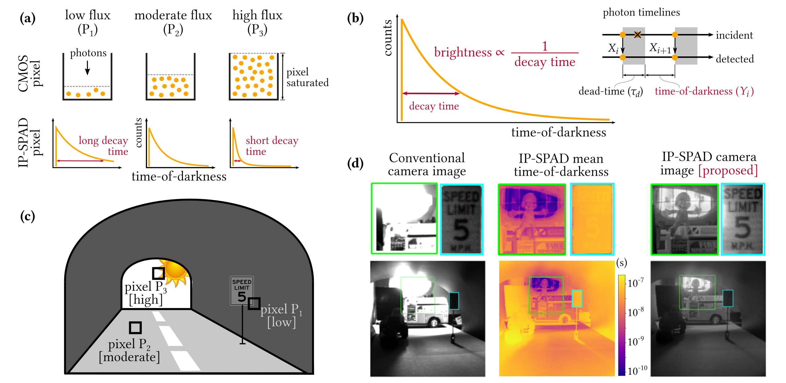
Figure 1: Passive imaging with an inter-photon single-photon avalanche diode (IP-SPAD): (a) A conventional image sensor pixel estimates scene brightness using a well-filling mechanism; the well has a finite capacity and saturates for very high brightness levels. (b) An IP-SPAD measures scene brightness from inter-photon timing measurements that follow Poisson statistics. The higher the brightness, the smaller the inter-photon time, the faster the decay rate of the inter-photon histogram. By capturing photon timing information with very high precision, this estimator can provide scene brightness estimates well beyond the saturation limit of conventional pixels. (c) A representative extreme dynamic range scene of a tunnel with three different flux levels (low, moderate and high) shown for illustration. (d) Experimental results from our hardware prototype comparing a conventional CMOS camera image and an image obtained from our IP-SPAD prototype.

How to Measure Inter-Photon Timing? The inter-photon timing intensity cue and the resulting brightness estimators can achieve extremely high dynamic range. A natural question to ask then is: How does one measure the inter-photon timing? Conventional CMOS sensor pixels do not have the ability to measure time delays between individual photons at the timing granularity needed for estimating intensities with high precision. Fortunately, there is an emerging class of sensors called single-photon avalanche diodes (SPADs) [11, 7], that can not only detect individual photons, but also precisely time-tag each captured photon with picosecond resolution.

Emergence of Single-Photon Sensors: SPADs are naturally suited for imaging in low illumination conditions, and thus, are fast becoming the sensors of choice for applications that require extreme sensitivity to photons together with fine-grained temporal information: single-photon 3D time-of-flight imaging [54, 34, 48, 47, 33], transient imaging [52, 51], non-line-of-sight imaging [35, 19], and fluorescence microscopy [43]. While these applications use SPADs in active imaging setups in synchronization with an illumination source such as a pulsed laser, recently these sensors have been explored as passive, general-purpose imaging devices for high-speed and high-dynamic range photography [4, 25, 36]. In particular, it was shown that SPADs can be used to measure incident flux while operating as passive, free-running pixels (PF-SPAD imaging) [25]. The dynamic range of the resulting measurements, although higher than conventional pixels (that rely on a finite-depth well filling light detection method like CCD and CMOS sensors), is inherently limited due to quantization stemming from the discrete nature of photon counts.

Intensity from Inter-Photon Timing: Our key idea is that it is possible to circumvent the limitations of counts-based photon flux estimation by exploiting photon timing information from a SPAD. The additional time-dimension is a rich source of information that is inaccessible to conventional photon count-based methods. We derive a scene brightness estimator that relies on the decay time statistics of the inter-photon times captured by a SPAD sensor as shown in Fig. 1(b). We call our image sensing method inter-photon SPAD (IP-SPAD) imaging. An IP-SPAD pixel captures the decay time distribution which gets narrower with increasing brightness. As shown in Fig. 1(d), the measurements can be summarized in terms of the mean time-of-darkness, which can then be used to estimate incident flux.

Unlike a photon-counting PF-SPAD pixel whose measurements are inherently discrete, an IP-SPAD measures decay times as floating point values, capturing information at much finer granularity than integer-valued counts, thus enabling measurement of extremely high flux values. In practice, the dynamic range of an IP-SPAD is limited only by the precision of the floating point representation used for measuring the time-of-darkness between consecutive photons. Coupled with the sensitivity of SPADs to individual photons and lower noise compared to conventional sensors, the proposed approach, for the first time, achieves ultra high-dynamic range. We experimentally demonstrate a dynamic range of over ten million to one, simultaneously imaging extremely dark (pixels P₁ and P₂ inside the tunnel in Fig. 1(c)) as well as very bright scene regions (pixel P₃ outside the tunnel in Fig. 1(c)).

2 Related Work

High-Dynamic-Range Imaging: Conventional high-dynamic-range (HDR) imaging techniques using CMOS image sensors use variable exposures to capture scenes with extreme dynamic range. The most common method called exposure bracketing [21, 22] captures multiple images with different exposure times; shorter exposures reliably capture bright pixels in the scene avoiding saturation, while longer exposures capture darker pixels while avoiding photon noise. Another technique involves use of neutral density (ND) filters of varying densities resulting in a tradeoff between spatial resolution and dynamic range [40]. ND filters reduce overall sensitivity to avoid saturation, at the cost of making darker scene pixels noisier. In contrast, an IP-SPAD captures scene intensities in a different way by relying on the non-linear reciprocal relationship between inter-photon timing and scene brightness. This gives extreme dynamic range in a single capture.

Passive Imaging with Photon-Counting Sensors: Previous work on passive imaging with photon counting sensors relies on two sensor technologies—SPADs and quanta-image sensors (QISs) [18]. A QIS has single-photon sensitivity but much lower time resolution than a SPAD pixel. On the other hand, QIS pixels can be designed with much smaller pixel pitch compared to SPAD pixels, allowing spatial averaging to further improve dynamic range while still maintaining high spatial resolution [36]. SPAD-based high-dynamic range schemes provide lower spatial resolution than the QIS-based counterparts [16], although, recently, megapixel SPAD arrays capable of passive photon counting have also be developed [39]. Previous work [25] has shown that passive free-running SPADs can potentially provide several orders of magnitude improved dynamic range compared to conventional CMOS image sensor pixel. The present work exploits the precise timing information, in addition to photon counts, measured by a free-running SPAD sensor. An IP-SPAD can image scenes with even higher dynamic range than the counts-based PF-SPAD method.

Methods Relying on Photon Timing: The idea of using timing information for passive imaging has been explored before for conventional CMOS image sensor pixels. A saturated CMOS pixel’s output is simply a constant and meaningless, but if the time taken to reach saturation is also available [13], it provides information about scene brightness, because a brighter scene point will reach saturation more quickly (on average) than a dimmer scene point. The idea of using photon timing information for HDR has also been discussed before but the dynamic range improvements were limited by the low timing resolution of the pixels [55, 31] at which point, the photon timing provides no additional information over photon counts. In their seminal work on single-photon 3D imaging under high illumination conditions, Rapp et al. provide rigorous theoretical derivations of photon-timing-based maximum-likelihood flux estimators that include dead-time effects of both the SPAD pixel and the timing electronics [45, 46]. Our theoretical SNR analysis and experimental results show that such photon-timing-based flux estimators can provide extreme dynamic range for passive 2D intensity imaging.

Methods Relying on Non-linear Sensor Response: Logarithmic image sensors include additional pixel electronics that apply log-compression to capture a large dynamic range. These pixels are difficult to calibrate and require additional pixel electronics compared to conventional CMOS image sensor pixels [27]. A modulo-camera [56] allows a conventional CMOS pixel output to wrap around after saturation. It requires additional in-pixel computation involving an iterative algorithm that unwraps the modulo-compression to reconstruct the high-dynamic-range scene. In contrast, our timing-based HDR flux estimator is a closed-form expression that can be computed using simple arithmetic operations. Although our method also requires additional in-pixel electronics to capture high-resolution timing information, recent trends in SPAD technology indicate that such arrays can be manufactured cheaply and at scale using CMOS fabrication techniques [24, 23].

Active Imaging Methods: Photon timing information captured by a SPAD sensor has been exploited for various active imaging applications like transient imaging [41], fluorescence lifetime microscopy [7], 3D imaging LiDAR [30, 20] and non-line-of-sight imaging [29, 9]. Active methods capture photon timing information with respect to a synchronized light source like a pulsed laser that illuminates the scene. In a low flux setting, photon timing information measured with respect to a synchronized laser source can be used to reconstruct scene depth and reflectivity maps [30]. In contrast, here we show that inter-photon timing information captured with an asynchronous SPAD sensor can enable scene intensity estimation not just in low but also extremely high flux levels in a passive imaging setting.

Figure 2: Comparison of noise sources in different image sensor pixels: (a) Theoretical expressions for the three main sources of noise affecting a conventional pixel, PF-SPAD pixel [25] and the proposed IP-SPAD pixel are summarized in this table. Note that the IP-SPAD’s sources of noise are similar to a PF-SPAD except for quantization noise. (b) The expressions in (a) are plotted for the case of $T=$5\text{\,}\mathrm{ms}\text{/}$$, $q=100\%$, $\sigma_{r}=5e^{-}$, $\Phi_{\text{dark}}=10$ photons/second, $\tau_{\text{d}}=$150\text{\,}\mathrm{ns}\text{/}$$, $\Delta=$200\text{\,}\mathrm{ps}\text{/}$$. The conventional sensor’s saturation capacity is set at 34,000 $e^{-}$ which matches the maximum possible SPAD counts of $\lceil\nicefrac{{T}}{{\tau_{\text{d}}}}\rceil$. Observe that the IP-SPAD soft-saturation point is at a much higher flux level than the PF-SPAD.

3 Image Formation with Inter-Photon Timing

3.1 Flux Estimator

Consider a single IP-SPAD pixel passively capturing photons over a fixed exposure time $T$ from a scene point with true photon flux of $\Phi$ photons per second. After each photon detection event, the IP-SPAD pixel goes blind for a fixed duration $\tau_{\text{d}}$ called the dead-time. During this dead-time, the pixel is reset and the pixel’s time-to-digital converter (TDC) circuit stores a picosecond resolution timestamp of the most recent photon detection time, and also increments the total photon count. This process is repeated until the end of the exposure time $T$. Let $N_{T}\geq 2$ denote the total number of photons detected by the IP-SPAD pixel during its fixed exposure time, and let $X_{i}$ $(1\leq i\leq N_{T})$ denote the timestamp of the $i^{\text{th}}$ photon detection. The measured inter-photon times between successive photons is defined as $Y_{i}:=X_{i+1}-X_{i}-\tau_{\text{d}}$ (for $1\leq i\leq N_{T}-1$). Note that $Y_{i}$’s follow an exponential distribution. It is tempting to derive a closed-from maximum likelihood photon flux estimator $\widehat{\Phi}$ for the true flux $\Phi$ using the log-likelihood function of the measured inter-photon times $Y_{i}$:

$$\vspace{-0.15in}\log l(q\Phi;Y_{1},\ldots,Y_{N_{T}-1})=\log\left(\prod_{i=1}^{N_{T}-1}q\Phi\,e^{-q\Phi Y_{i}}\right)$$

$$=-q\Phi\left(\sum_{n=1}^{N_{T}-1}Y_{i}\right)+(N_{T}-1)\log q\Phi,\vspace{-0.15in}$$ (1)

where $0\!\!<q<\!\!1$ is the quantum efficiency of the IP-SPAD pixel. The maximum likelihood estimate $\widehat{\Phi}$ of the true photon flux is computed by setting the derivative of Eq. (1) to zero and solving for $\Phi$:

$$\boxed{\widehat{\Phi}=\frac{1}{q}\frac{N_{T}-1}{X_{N_{T}}-X_{1}-(N_{T}-1)\tau_{\text{d}}}.}$$ (2)

Although the above proof sketch captures the intuition of our flux estimator, it leaves out two details. First, the total number of photons $N_{T}$ is itself a random variable. Second, the times of capture of future photons are constrained by the timestamps of preceding photon arrivals because we operate in a finite exposure time $T$. The sequence of timestamps $Y_{i}$ cannot be treated as independent and identically distributed. In fact, it is possible to show that the sequence of timestamps forms a Markov chain [45] where the conditional distribution of the $i^{\text{th}}$ inter-photon time conditioned on the previous inter-photon times is given by:

$$p_{Y_{i}|Y_{1},\dots,Y_{i-1}}(t)=\begin{cases}q\Phi e^{-q\Phi t}&0<t<T_{i}\\ e^{-q\Phi T_{i}}\delta(t-T_{i})&t=T_{i}\\ 0&\mbox{otherwise.}\end{cases}$$

Here $\delta(\cdot)$ is the Dirac delta function. The $T_{i}$’s model the shrinking effective exposure times for subsequent photon detections. $T_{1}=T$ and for $i>1$, $T_{i}=\max(0,T_{i-1}-Y_{i-1}-\tau_{\text{d}})$. The log-likelihood function can now be written as:

$$\log l(q\Phi;Y_{1},\ldots,Y_{L})=\log\left(\prod_{i=1}^{\lceil\nicefrac{{T}}{{\tau_{\text{d}}}}\rceil}p_{Y_{i}|Y_{1},\dots,Y_{i-1}}(t)\right)$$

$$\!\!=-q\Phi\max\left(\sum_{i=1}^{N_{T}}Y_{i},T\!-\!N_{T}\tau_{\text{d}}\right)+N_{T}\log q\Phi.$$

As shown in Supplementary Note 1 this likelihood function also leads to the flux estimator given in Eq. (2).

We make the following key observations about the IP-SPAD flux estimator. First, note that the estimator is only a function of the first and the last photon timestamps, the exact times of capture of the intermediate photons do not provide additional information. This is because photon arrivals follow Poisson statistics: the time until the next photon arrival from the end of the previous dead-time is independent of all preceding photon arrivals. Secondly, we note that the denominator in Eq. (2) is simply the total time the IP-SPAD spends waiting for the next photon to be captured while not in dead-time. Intuitively, if the photon flux were extremely high, we will expect to see a photon immediately after every dead-time duration ends, implying the denominator in Eq. (2) approaches zero, hence $\widehat{\Phi}\rightarrow\infty$.

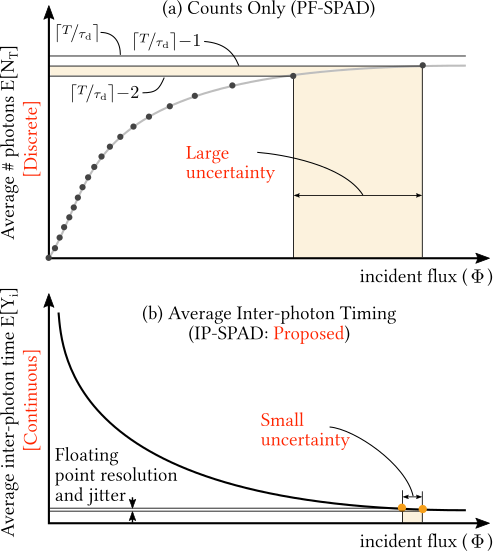
Figure 3: Advantage of using photon timing over photon counts: (a) Photon counts are inherently discrete. At high flux levels, even a small $\pm 1$ change in photon counts corresponds to a large flux uncertainty. (b) Inter-photon timing is inherently continuous. This leads to smaller uncertainty at high flux levels. The uncertainty depends on jitter and floating point resolution of the timing electronics.

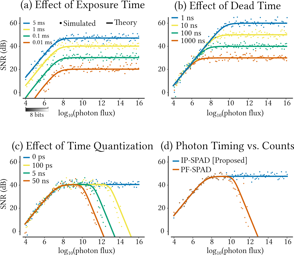
Figure 4: Effect of various IP-SPAD parameters on SNR: We vary different parameters to see the effect on SNR. The solid lines are theoretical SNR curves while each dot represents a SNR average from 10 Monte Carlo simulations. Unless otherwise noted the parameters used are $T=1$ $\mathrm{ms}\text{/}$, $\tau_{\text{d}}=100$ $\mathrm{ns}\text{/}$, $q=0.4$, and $\Delta=0$. (a) As exposure time increases, SNR increases at all brightness levels. (b) Decreasing the dead-time increases the maximum achievable SNR, but provides little benefit in low flux. (c) Coarser time quantization causes SNR drop-off at high flux values. (d) Our IP-SPAD flux estimator outperforms a counts-only (PF-SPAD) flux estimator [25] at high flux levels.

3.2 Sources of Noise

Although, theoretically, the IP-SPAD scene brightness estimator in Eq. (2) can recover the entire range of incident photon flux levels, including very low and very high flux values, in practice, the accuracy is limited by various sources of noise. To assess the performance of this estimator, we use a signal-to-noise ratio (SNR) metric defined as [53, 25]:

$$\mathsf{SNR}(\Phi)=10\log_{10}\left(\frac{\Phi^{2}}{\mathbf{E}[(\Phi-\widehat{\Phi})^{2}]}\right)$$ (3)

Note that the denominator in Eq. (3) is the mean-squared-error of the estimator $\widehat{\Phi}$, and is equal to the sum of the bias-squared terms and variances of the different sources of noise. The dynamic range (DR) of the sensor is defined as the range of brightness levels for which the SNR stays above a minimum specified threshold. At extremely low flux levels, the dynamic range is limited due to IP-SPAD dark counts which causes spurious photon counts even when no light is incident on the pixel. This introduces a bias in $\widehat{\Phi}$. Since photon arrivals are fundamentally stochastic (due to the quantum nature of light), the estimator also suffers from Poisson noise which introduces a non-zero variance term. Finally, at high enough flux levels, the time discretization $\Delta$ used for recording timestamps with the IP-SPAD pixel limits the maximum usable photon flux at which the pixel can operate. Fig. 2(a) shows the theoretical expression for bias and variance introduced by shot noise, quantization noise and dark noise in an IP-SPAD pixel along with corresponding expressions for a conventional image sensor pixel and a PF-SPAD pixel. Fig. 2(b) shows example plots for these theoretical expressions. For realistic values of $\Delta$ in the 100’s of picoseconds range, the IP-SPAD pixel has a smaller quantization noise term that allows reliable brightness estimation at much higher flux levels than a PF-SPAD pixel. (See Supplementary Note 2).

Figure 5: Simulated HDR scene captured with a PF-SPAD (counts only) vs. IP-SPAD (inter-photon timing): (a) Although a PF-SPAD can capture this extreme dynamic range scene in a single $5\text{\,}\mathrm{ms}\text{/}$ exposure, extremely bright pixels such as the bulb filament that are beyond the soft-saturation limit appear noisy. (b) An IP-SPAD camera captures both dark and bright regions in a single exposure, including fine details around the bright bulb filament. In both cases, we set the SPAD pixel’s quantum efficiency to 0.4, dead-time to $150\text{\,}\mathrm{ns}\text{/}$ and an exposure time of $5\text{\,}\mathrm{ms}\text{/}$. The IP-SPAD has a time resolution of $\Delta=$200\text{\,}\mathrm{ps}\text{/}$$. (Original image from HDRIHaven.com)

Quantization Noise in PF-SPAD vs. IP-SPAD: Conventional pixels are affected by quantization in low flux and hard saturation (full-well capacity) limit in high flux. In contrast, a PF-SPAD pixel that only uses photon counts is affected by quantization noise at extremely high flux levels due to soft-saturation [25]. This behavior is unique to SPADs and is quite different from conventional sensors. A counts-only PF-SPAD pixel can measure at most $\lceil\nicefrac{{T}}{{\tau_{\text{d}}}}\rceil$ photons where $T$ is the exposure time and $\tau_{\text{d}}$ is the dead-time [25]. Due to a non-linear response curve, as shown in Fig. 3(a), a small change of $\pm 1$ count maps to a large range of flux values. Due to the inherently discrete nature of photon counts, even a small fluctuation (due to shot noise or jitter) can cause a large uncertainty in the estimated flux.

The proposed IP-SPAD flux estimator uses timing information which is inherently continuous. Even at extremely high flux levels, photon arrivals are random and due to small random fluctuations, the time interval between the first and last photon ($X_{N_{T}}-X_{1}$) is not exactly equal to $T$. Fig. 3(b) shows the intuition for why fine-grained inter-photon measurements at high flux levels can enable flux estimation with a smaller uncertainty than counts alone. In practice, the improvement in dynamic range compared to a PF-SPAD depends on the time resolution, which is limited by hardware constraints like floating point precision of the TDC electronics and timing jitter of the SPAD pixel. Simulations in Fig. 4 suggest that even with a $100\text{\,}\mathrm{ps}\text{/}$ time resolution the 20-dB dynamic range improves by 2 orders of magnitude over using counts alone.

Single-Pixel Simulations: We verify our theoretical SNR expression using single-pixel Monte Carlo simulations of a single IP-SPAD pixel. For a fixed set of parameters we run 10 simulations of an IP-SPAD at 100 different flux levels ranging $10^{4}-10^{16}$ photons per second. Fig. 4 shows the effect of various pixel parameters on the SNR. The overall SNR can be increased by either increasing the exposure time $T$ or decreasing the dead-time $\tau_{\text{d}}$; both enable the IP-SPAD pixel to capture more total photons. The maximum achievable SNR is theoretically equal to $10\log_{10}\left(\nicefrac{{T}}{{\tau_{\text{d}}}}\right)$. The IP-SPAD SNR degrades at high flux levels due because photon timestamps cannot be captured with infinite resolution. A larger floating point quantization bin size $\Delta$ increases the uncertainty in photon timestamps. If the time bin is large enough, there is no advantage in using the timestamp-based brightness estimator and the performance reverts to a counts-based flux estimator [4, 25].

4 Results

4.1 Simulation Results

Simulated RGB Image Comparisons: Fig. 5 shows a simulated HDR scene with extreme brightness variations between the dark text and bright bulb filament. We use a $5\text{\,}\mathrm{ms}\text{/}$ exposure time for this simulation. The PF-SPAD and IP-SPAD both use pixels with $q=0.4$ and $\tau_{\text{d}}=$150\text{\,}\mathrm{ns}\text{/}$$. The PF-SPAD only captures photon counts whereas the IP-SPAD captures counts and timestamps with a resolution of $\Delta=$200\text{\,}\mathrm{ps}\text{/}$$. Notice that the extremely bright pixels on the bulb filament appear noisy in the PF-SPAD image. This degradation in SNR at high flux levels is due to its soft-saturation phenomenon. The IP-SPAD, on the other hand, captures the dark text and noise-free details in the bright bulb filament in a single exposure. Please see supplement for additional comparisons with a conventional camera.

Figure 6: Experimental “Tunnel” scene: (a-b) Images from a conventional sensor with long and short exposure times. Notice that both the speed limit sign and the toy figure cannot be captured simultaneously with a single exposure. Objects outside the tunnel appear saturated even with the shortest exposure time possible with our CMOS camera. (c) A PF-SPAD [25] only uses photon counts when estimating flux. Although it captures much higher dynamic range than the conventional CMOS camera, the bright pixels near the halogen lamp appear saturated. (d) Our IP-SPAD single-pixel hardware prototype captures both the dark and the extremely bright regions with a single exposure. Observe that the fine details within the halogen lamp are visible.

4.2 Single-Pixel IP-SPAD Hardware Prototype

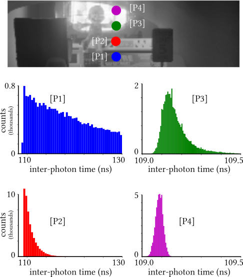
Figure 7: Rise-time Non-ideality in Measured IP-SPAD Histograms: We show four inter-photon histograms for pixels in the experimental “Tunnel” scene. The histograms of [P1] and [P2] have an ideal exponentially decaying shape. However, at the brighter points, [P3] and [P4], the inter-photon histograms deviate from an ideal exponential shape. This is because the IP-SPAD pixels requires $\sim$100\text{\,}\mathrm{ps}\text{/}$$ rise time to re-activate after the end of the previous dead-time.

Our single-pixel IP-SPAD prototype is a modified version of a fast-gated SPAD module [8]. Conventional dead-time control circuits for a SPAD rely on digital timers that have a coarse time-quantization limited by the digital clock frequency and cannot be used for implementing an IP-SPAD. We circumvent this limitation by using coaxial cables and low-jitter voltage comparators to generate “analog delays” that enable precise control of the dead-time with jitter limited to within a few $\mathrm{ps}\text{/}$. We used a $20\text{\,}\mathrm{m}\text{/}$ long co-axial cable to get a dead-time of $110\text{\,}\mathrm{ns}\text{/}$. The measured dead-time jitter was $\sim$200\text{\,}\mathrm{ps}\text{/}$$. This is an improvement over previous PF-SPAD implementations [25] that relied on a digital timer circuit whose time resolution was limited to $\sim$6\text{\,}\mathrm{ns}\text{/}$$.

The IP-SPAD pixel is mounted on two translation stages that raster scan the image plane of a variable focal length lens. The exposure time per pixel position depends on the translation speed along each scan-line. We capture 400$\times$400 images with an exposure time of $5$ $\mathrm{ms}\text{/}$ per pixel position. The total capture takes $\sim\!\!\!15$ minutes. Photon timestamps are captured with a $1\text{\,}\mathrm{ps}\text{/}$ time binning using a time-correlated single-photon counting (TCSPC) system (PicoQuant HydraHarp400). A monochrome camera (PointGrey Technologies GS3-U3-23S6M-C) placed next to the SPAD captures conventional camera images for comparison. The setup is arranged carefully to obtain approximately the same field of view and photon flux per pixel for both the IP-SPAD and CMOS camera pixels.

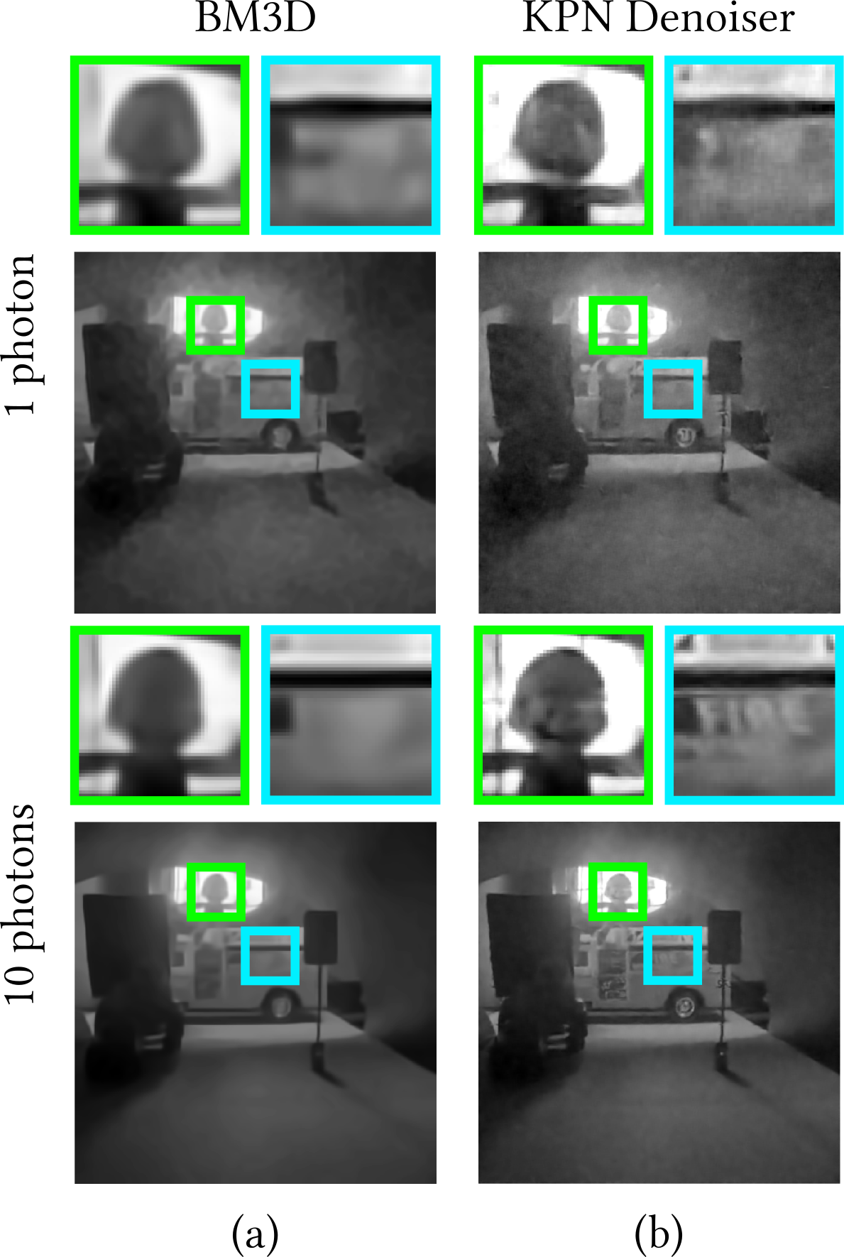
Figure 8: IP-SPAD Imaging in Low Photon Count Regime: This figure shows IP-SPAD images captured with very few photons and denoised with two different methods: (a) an off-the-shelf BM3D denoiser, and (b) a DNN denoiser based on a kernel prediction network architecture. Details like the text on the fire-truck are visible with as few as 10 photons per pixel.

4.3 Hardware Experiment Results

HDR Imaging: Fig. 6 shows an experiment result using our single-pixel raster-scanning hardware prototype. The “Tunnel” scene contains dark objects like a speed limit sign inside the tunnel and an extremely bright region outside the tunnel from a halogen lamp. This scene has a dynamic range of over $1\text{\times}{10}^{7}$:$1$. The conventional CMOS camera (Fig. 6(a-b)), requires multiple exposures to cover this dynamic range. Even with the shortest possible exposure time of $0.005\text{\,}\mathrm{ms}\text{/}$, the halogen lamp appears saturated. Our IP-SPAD prototype captures details of both the dark regions (text on the speed limit sign) simultaneously with the bright pixels (outline of halogen lamp tube) in a single exposure. Fig. 6(c) and (d) shows experimental comparison between a PF-SPAD (counts-only) image [25] and the proposed IP-SPAD image that uses photon timestamps. Observe that in extremely high flux levels (in pixels around the halogen lamp) the PF-SPAD flux estimator fails due to the inherent quantization limitation of photon counts. The IP-SPAD preserves details in these extremely bright regions, like the shape of the halogen lamp tube and the metal cage on the lamp.

Hardware Limitations: The IP-SPAD pixel does not exit the dead-time duration instantaneously and in practice it takes around $100\text{\,}\mathrm{ps}\text{/}$ to transition into a fully-on state. Representative histograms for four different locations in the experiment tunnel scene are shown in Fig. 7. Observe that at lower flux levels (pixels [P1] and [P2]) the inter-photon histograms follow an exponential distribution as predicted by the Poisson model for photon arrival statistics. However, at pixels with extremely high brightness levels (pixels [P3] and [P4] on the halogen lamp), the histograms have a rising edge denoting the transition phase when the pixel turns on after the end of the previous dead-time. We also found that in practice the dead-time is not constant and exhibits a drift over time (especially at high flux values) due to internal heating. Such non-idealities, if not accounted for, can cause uncertainty in photon timestamp measurements, and limit the usability of our flux estimator in the high photon flux regime. Since we capture timestamps for every photon detected in a fixed exposure time, it is possible to correct these non-idealities in post-processing by estimating the true dead-time and rise-time from these inter-photon timing histograms. See Supplementary Note 5 for details.

IP-SPAD Imaging with Low Photon Counts: The results so far show that precise photon timestamps from an IP-SPAD pixel enables imaging at extremely high photon flux levels. We now show that it is also possible to leverage timing information when the IP-SPAD pixel captures very few photons per pixel. We simulate the low photon count regime by keeping the first few photons and discarding the remaining photon timestamps for each pixel in the experimental “Tunnel” scene. Fig. 8 shows IP-SPAD images captured with as few as 1 and 10 photons per pixel and denoised using an off-the-shelf BM3D denoiser and a deep neural network denoiser that uses a kernel prediction network (KPN) architecture [38]. We can recover intensity images with just one photon timestamp per pixel using real data captured by our IP-SPAD hardware prototype. Quite remarkably, with as few as 10 photons per pixel, image details such as facial features and text on the fire truck are discernible. Please see Supplementary Note 3 for details about the KPN denoiser and Supplementary Note 6 for additional experimental results and comparisons with other denoising algorithms.

5 Future Outlook

The analysis and experimental proof-of-concept shown in this paper were restricted to a single IP-SPAD pixel. Recent advances in CMOS SPAD technology that rely on 3D stacking [23] can enable larger arrays of SPAD pixels for passive imaging. This will introduce additional design challenges and noise sources not discussed here. In Supplementary Note 7 we show some pixel architectures for an IP-SPAD array that could be implemented in the future.

Arrays of single-photon image sensor pixels are being increasingly used for 2D intensity imaging and 3D depth sensing [54, 32, 37] in commercial and consumer devices. When combined with recent advances in high-time-resolution SPAD sensor hardware, the methods developed in this paper can enable extreme imaging applications across various applications including consumer photography, vision sensors for autonomous driving and robotics, and biomedical optical imaging.

Supplementary Note 1 Image Formation

Supplementary Figure 1: Photon Detection Timeline: (a) The photon timeline shows the random variables used in the derivation of our photon flux estimator. $X_{i}$’s denote the photon arrival time with respect to the start of the exposure at $t=0$ and $Y_{i}$’s denote the $i^{th}$ time-of-darkness. (b) There are two possibilities for the final dead-time window after the last photon detection. In high photon flux scenarios, the final dead-time ends after the end of the exposure time $(X_{N_{T}}+\tau_{\text{d}}>T)$ with high probability.

Consider an IP-SPAD sensor pixel with quantum efficiency $q$ exposed to a photon flux of $\Phi$ photons/second. Photon arrivals follow a Poisson process, so inter-photon times follow an exponential distribution with rate $q\Phi$. After a detection event the IP-SPAD is unable to detect photons for a period of $\tau_{\text{d}}$. Because of the memoryless property of a Poisson process, the arrival time of a photon after the end of a dead-time window (called the time-of-darkness), follows an exponential distribution with rate $q\Phi$. The probability that no photons are detected in the exposure time $T$ is equal to $\int^{\infty}_{T}q\Phi e^{-q\Phi t}dt=e^{-q\Phi T}.$

Let the first time-of-darkness be denoted by $Y_{1}$. If no photons are detected, we define $Y_{1}:=T$. If $Y_{1}<T$ it follows an exponential distribution. Therefore, the probability density function of $Y_{1}$ can be written as:

$$Y_{1}{\sim}f_{Y_{1}}(t)=\begin{cases}q\Phi e^{-q\Phi t}&\mbox{for }0<t<T\\ e^{-q\Phi T}\delta(t-T)&\mbox{for }t=T\\ 0&\mbox{otherwise,}\end{cases}$$ (S1)

where $\delta$ is the Dirac delta function.

Now consider $Y_{2}$, the second time-of-darkness. $Y_{2}$ is non-zero if and only if $Y_{1}\neq T$ (to be the second, there must be a first). If the second photon is detected, $Y_{2}$ will be exponentially distributed. But the exposure time interval shrinks because a time interval of $Y_{1}+\tau_{\text{d}}$ has elapsed due to the first photon detection. We define the remaining exposure time $T_{2}=\max(0,T-Y_{1}-\tau_{d}$), where the $\max()$ function ensures $T_{2}$ is non-negative. Then the probability distribution of $Y_{2}$ conditioned on $Y_{1}$ will be given by replacing $T$ for $T_{2}$ in Eq. (S1). More generally, the conditional distribution of $Y_{i}$ can be written as:

$$Y_{i}\sim f_{Y_{i}|Y_{1}\dots Y_{i-1}}(t|Y_{1}\dots Y_{i-1})=\begin{cases}q\Phi e^{-q\Phi t}&\mbox{for }0<t<T_{i}\\ e^{-q\Phi T_{i}}\delta(t-T_{i})&\mbox{for }t=T_{i}\\ 0&\mbox{otherwise,}\end{cases}$$ (S2)

where,

$$T_{1} =T$$

$$T_{i} =\max(0,T_{i-1}-Y_{i-1}-\tau_{\text{d}}))$$

$$=\max\left(0,T-\sum^{i-1}_{j=1}(Y_{j}+\tau_{\text{d}})\right).$$ (S3)

The $T_{i}$’s model the fact that the effective exposure time for the $i^{th}$ photon shrinks due to preceding photon detections. Note if $Y_{i}=T_{i}$ then no $i^{\text{th}}$ photon is detected and $Y_{i+1}=T_{i+1}=0$. Note that the $X_{i}$ in the main text are related to $Y_{i}$ by $X_{i}-X_{i-1}-\tau_{\text{d}}=:Y_{i}$ for $i\geq 2$ and $X_{1}=Y_{1}$. Suppl. Fig. 1(a) shows $X_{i}$ and $Y_{i}$ on a photon timeline.

Maximum Likelihood Flux Estimator

For a fixed exposure time $T$, the maximum number of possible photon detections is $L=\big{\lceil}\frac{T}{\tau_{\text{d}}}\big{\rceil}$. Let $N$ be the number of detected photons, then $Y_{N+1}$ will be the last possibly non-zero time-of-darkness, and $Y_{N+2}\dots Y_{L}=0$ with probability $1$. The log-likelihood of the unknown flux value given the set of time-of-darkness measurements $Y_{1}\dots Y_{L}$ is given by:

$$\log l(q\Phi;Y_{1},\ldots,Y_{L}) =\log\left(\prod_{i=1}^{L}f_{Y_{i}}(Y_{i}|Y_{1}\dots Y_{i-1})\right)$$

$$=\log\left(f_{Y_{N+1}}(Y_{N+1}|Y_{1}\dots Y_{N})\prod_{i=1}^{N}f_{Y_{i}}(Y_{i}|Y_{1}\dots Y_{i-1})\right)$$

$$=\log\left(e^{-q\Phi T_{N+1}}\prod_{i=1}^{N}q\Phi\,e^{-q\Phi Y_{i}}\right)$$

$$=-q\Phi\left(T_{N+1}+\sum_{i=1}^{N}Y_{i}\right)+N\log q\Phi$$

$$=-q\Phi\,\left(\max\left(0,T-\sum_{i=1}^{N}Y_{i}-\tau_{\text{d}}\right)+\sum_{i=1}^{N}Y_{i}\right)+N\log q\Phi$$

$$=-q\Phi\,\max\left(\sum_{i=1}^{N}Y_{i},T-N\tau_{\text{d}}\right)+N\log q\Phi.$$ (S4)

We find the maximum likelihood estimate, $\widehat{\Phi}$, by setting the derivative of Eq.(S4) to zero and solving for $\Phi$:

$$-q\max\left(\sum_{i=1}^{N}Y_{i},T-N\tau_{\text{d}}\right)+\frac{N}{\widehat{\Phi}} =0,$$ (S5)

which gives:

$$\widehat{\Phi}=\frac{N}{q\max\left(\sum_{n=1}^{N}Y_{i},T-N\tau_{\text{d}}\right)}.$$ (S6)

The $\max()$ function can be thought of as selecting the time-of-darkness based on whether or not the final dead-time window ends after $t=T$, see Suppl. Fig. 1(b). In practice the beginning and end of the exposure time may not be known precisely, introducing uncertainty in $X_{1}$ and $T$. Because of this we instead use an approximation:

$$\widehat{\Phi}=\frac{N-1}{q\sum_{n=2}^{N}Y_{i}}.$$ (S7)

Plugging in $Y_{i}=X_{i}-X_{i-1}-\tau_{\text{d}}$ gives Eq. (2) in the main text.

Flux Estimator Variance

Let $N$ be the number of photons detected in an exposure time $T$. Using the law of large numbers for renewal processes we find the expectation and the variance of $N$ to be:

$$\text{E}[N]=\frac{q\Phi(T+\tau_{\text{d}})}{1+q\Phi\tau_{\text{d}}}$$ (S8)

$$\text{Var}[N]=\frac{q\Phi(T+\tau_{\text{d}})}{(1+q\Phi\tau_{\text{d}})^{3}}$$ (S9)

In the following derivation we will assume $N$ is large enough that it can be assumed to be constant for a given $T$. This holds, for example, when $\Phi\gg\frac{1}{T}$. This assumption also allows us to approximate $Y_{i}$’s as i.i.d. shifted exponential random variables. We will consider the estimator in Eq. (S7) where the sum in the denominator is given by $S_{N_{T}}=Y_{2}+Y_{3}+...Y_{N}$ and letting $N_{T}=N-1$. The final photon timestamp $S_{N_{T}}$ is the sum of exponential random variables and follows a gamma distribution:

$$S_{N_{T}}\stackrel{{\scriptstyle}}{{\sim}}f_{S_{N_{T}}}(t)=\begin{cases}\frac{(q\Phi)^{N_{T}}t^{N_{T}-1}e^{-q\Phi t}}{(N_{T}-1)!}&\mbox{for }t\geq 0\\ 0&\mbox{otherwise.}\end{cases}$$ (S10)

The mean of $\widehat{\Phi}$ can be computed as:

$$\text{E}\left[\frac{N_{T}}{qS_{N_{T}}}\right] =\frac{N_{T}}{q}\text{E}\left[\frac{1}{S_{N_{T}}}\right]$$

$$=\frac{N_{T}}{q}\int^{\infty}_{0}\frac{(q\Phi)^{N_{T}}t^{N_{T}-1}e^{-q\Phi t}}{t(N_{T}-1)!}\,dt$$

$$=\frac{N_{T}}{q}\frac{q\phi}{N_{T}-1}\int^{\infty}_{0}\frac{(q\Phi)^{N_{T}-1}t^{N_{T}-2}e^{-q\Phi t}}{(N_{T}-2)!}\,dt$$

$$=\frac{N_{T}}{N_{T}-1}\Phi$$ (S11)

where the last line comes from the recognizing the argument of the integral as the p.d.f. for a gamma distribution and for large $N_{T}$, $\frac{N_{T}}{N_{T}-1}\approx 1$.

The second moment of $\widehat{\Phi}$ is given by:

$$\text{E}\left[\left(\frac{N_{T}}{qS_{N_{T}}}\right)^{2}\right] =\frac{N_{T}^{2}}{q^{2}}\text{E}\left[\frac{1}{S_{N_{T}}^{2}}\right]$$

$$=\frac{N_{T}^{2}}{q^{2}}\int^{\infty}_{0}\frac{(q\Phi)^{N_{T}}t^{N_{T}-1}e^{-q\Phi t}}{t^{2}(N_{T}-1)!}dt$$

$$=\frac{(q\Phi)^{2}N_{T}^{2}}{q^{2}(N_{T}-1)(N_{T}-2)}\int^{\infty}_{0}\frac{(q\Phi)^{N_{T}-2}t^{N_{T}-3}e^{-q\Phi t}}{(N_{T}-3)!}dt$$

$$=\frac{\Phi^{2}N_{T}^{2}}{(N_{T}-1)(N_{T}-2)}$$ (S12)

This expression is valid for $N_{T}>2$. The variance of $\widehat{\Phi}$ is given by:

$$\text{Var}\left[\frac{N_{T}}{qS_{N_{T}}}\right] =\Phi^{2}\frac{N_{T}^{2}}{(N_{T}-2)(N_{T}-1)}-\frac{N_{T}^{2}}{(N_{T}-1)^{2}}\Phi^{2}$$

$$=\Phi^{2}\frac{N_{T}^{2}}{(N_{T}-2)(N_{T}-1)^{2}}$$

$$\approx\Phi^{2}\frac{1}{N_{T}}$$ (S13)

$$=\Phi^{2}\frac{q\Phi\tau_{\text{d}}+1}{q\Phi(T+\tau_{\text{d}})}$$ (S14)

$$\approx\Phi\frac{q\Phi\tau_{\text{d}}+1}{qT}$$ (S15)

where we replace $N_{T}$ with its mean value. The last line follows if we assume $T\gg\tau_{\text{d}}$. Finally, the SNR is given by:

SNR $$=20\log_{10}\frac{\Phi}{\sqrt{\text{Var}[\frac{N_{T}}{qS_{N_{T}}}]}}$$

$$=10\log_{10}\frac{q\Phi T}{q\Phi\tau_{\text{d}}+1}$$ (S16)

We make the following observations about our estimator $\widehat{\Phi}$:

• At high flux, when $N_{T}$ is large enough, Eq. (S11) reduces to $\text{E}[\widehat{\Phi}]=\Phi$, i.e. our estimator is unbiased.

• Unlike [25] which only uses photon counts $N_{T}$, our derivation explicitly accounts for individual inter-photon timing information captured in $S_{N_{T}}$.

• As $\Phi\rightarrow\infty$, $\text{SNR}\rightarrow 10\log_{10}(\frac{T}{\tau_{\text{d}}})$. So at high flux the SNR will flatten out to a constant independent of the true flux $\Phi$. In practice, the SNR drops at high flux due to time quantization, discussed next in Supplementary Note 2.

Supplementary Note 2 Time Quantization

Consider an IP-SPAD with quantum efficiency $q$, dead time $\tau_{\text{d}}$, and time quantization $\Delta$ that detects photons over exposure time $T$. To match our hardware prototype, the start of the dead time window is not quantized and time stamps are quantized by $\Delta$. The quantization noise variance term derived in previous work [25, 4] that relies on a counts-only measurement model is given by:

$$V_{\text{count-quantization}}=\frac{(1+q\Phi\tau_{\text{d}})^{4}}{12q^{2}T^{2}}.$$ (S17)

We derive a modified quantization noise variance expression by modifying this counts-only expression to account for two key insights gained from extensive simulations of SNR plots for our timing-based IP-SPAD flux estimator. First, we note that the timing-based IP-SPAD flux estimator follows a similar SNR curve as the counts-based PF-SPAD flux estimator when $\Delta=\tau_{\text{d}}$. Second, the rate at which the SNR drop off moves slows after $\Delta$ exceeds $\tau_{\text{d}}$. In this way we propose a new time quantization term:

$$V_{\text{time-quantization}}=\frac{(1+q\Phi\tau_{\text{d}}+q\Phi\Delta)^{2}(1+q\phi\Delta)^{2}}{12q^{2}T^{2}}.$$ (S18)

Note we break the quartic term from Eq. (S17) into two quadratic terms. The two quadratic terms strike a balance between quantization due to counts and timing. If $\Delta=0$ then $V_{\text{time quantization}}$ is an order 2 polynomial with respect to $\Phi$ which leads to a constant SNR at high flux. Also note if $\Delta=\tau_{\text{d}}$ the time quantization term is roughly equal to the counts quantization term. We found this expression matches simulated IP-SPAD SNR curves for a range of dead-times and exposure times.

Supplementary Note 3 IP-SPAD Imaging with Low Photon Counts

The scene brightness estimator (Eq. (2)) requires the IP-SPAD pixel to capture at least two photons; It does not make sense to talk about “inter-photon” times with only one photon. The situation where an IP-SPAD pixel captures only one incident photon timestamp can be thought of as an extreme limiting case of passive inter-photon imaging under low illumination.

Intuitively, we can reconstruct an image from a single photon timestamp per pixel by simply computing the reciprocal of the first photon timestamp at each pixel. Brighter scene points should have a smaller first-photon timestamp (on average) because, with high probability, a photon will be detected almost immediately after the pixel starts collecting light. In this supplementary note we show that the conditional distribution of this first photon timestamp (conditioned on there being at least one photon detection) is a uniform random variable:

$$\{Y_{1}|Y_{1}\leq T\}\sim\mathcal{U}[0,T].$$

when operating under low incident photon flux. This implies that timestamps provide no additional information beyond merely the fact that at least one photon was detected. We must, therefore, relax the requirement of a constant exposure time and allow each pixel to capture at least one photon by allowing variable exposure times per pixel. When operated this way, first-photon timestamps do carry useful information about the scene brightness. The estimate of the scene pixel brightness is given by $\widehat{\Phi}=\nicefrac{{1}}{{q\,Y_{i}}}$.

When the total number of photons is extremely small, the information contained in the timestamp data is extremely noisy. We leverage spatial-priors-based image denoising techniques that have been developed for conventional images, and adapt them denoising these noisy IP-SPAD images. Coupled with the inherent sensitivity of SPADs, this enables us to reconstruct intensity images with just a single photon per pixel [26].

In this section we show that for passive imaging in the low photon flux regime with a constant exposure time per pixel, the timestamp of the first arriving photon is a uniform random variable and hence, carries no useful information about the true photon flux. If we drop the constant exposure time constraint and instead operate in a regime where each pixel is allowed to wait until the first photon is captured (random exposure time per pixel), then the first-photon timestamps carry useful information about the flux, albeit noisy.

Supplementary Note 3.1 When Do Timestamps Carry Useful Information?

Let us assume an IP-SPAD pixel operating with a fixed exposure time $T$ is observing a scene point with photon flux $\Phi$. We assume that the photon flux is low enough so that the pixel captures at most one photon during this exposure time. The (random) first-photon arrival time is denoted by $Y_{1}$ as shown in Suppl. Fig. 2. We would like to know if the first photon time-of-arrival carries useful information about $\Phi$.

Supplementary Figure 2: We capture the first arriving photon and record its arrival time in a fixed exposure time T. Note that in the low photon flux regime $\Phi T\ll 1$, so there is a high probability that zero photons are detected in the time interval $[0,T]$.

We derive the probability distribution of $Y_{1}$, conditioning on $Y_{1}\leq T$. For any $t>0$,

$$P(Y_{1}\leq t|Y_{1}\leq T) =\frac{P(Y_{1}\leq t\cap Y_{1}\leq T)}{P(Y_{1}\leq T)}$$ (S19)

$$=\frac{P(Y_{1}\leq t)}{P(Y_{1}\leq T)}$$ (S20)

$$=\frac{1-e^{-\Phi t}}{1-e^{-\Phi T}}$$ (S21)

where Eq. (S19) follows from Bayes’s rule, Eq. (S20) assumes $t\leq T$ (otherwise the answer is 1, trivially) and Eq. (S21) is obtained by plugging in the c.d.f. of $Y_{1}\sim\text{Exp}(\Phi).$

Due to the low flux assumption, $\Phi\ll\frac{1}{T}$. Then $\Phi t\leq\Phi T\ll 1$ and we can approximate $1-e^{-\Phi T}\approx\Phi T$ and $1-e^{-\Phi t}\approx\Phi t$. This gives

$$P(Y_{1}\leq t|Y_{1}\leq T)=\frac{t}{T}$$ (S22)

which is the c.d.f. of a uniform random variable. This implies that, in the low photon flux regime the arrival time distribution converges weakly to a uniform random variable:

$$\{Y_{1}|Y_{1}\leq T\}\overset{D}{\rightarrow}\mathcal{U}[0,T].$$

For low illumination conditions, we drop the requirement of a fixed exposure time and allow the IP-SPAD pixel to wait until the first photon timestamp is captured.

Supplementary Note 3.2 KPN-based Denoising Network for Low Light IP-SPAD Imaging

In principle, any standard neighborhood-based image denoising algorithm (e.g., bilateral filtering [42] and BM3D [15]) can be applied to the IP-SPAD images captured in a low photon count regime. But the heavy-tailed nature of the timestamps poses problems to off-the-shelf denoising algorithms as they usually assume a light-tailed distribution of pixel intensities (e.g., Gaussian distribution). A solution to this issue is the use of a variance-stabilizing Anscombe transform [3] to make the noise variance uniform across the whole image. For photon timestamp data, the variance-stabilizing transform is the logarithm. See Supplementary Note 3.3 for a proof. We design an image denoising deep neural network (DNN) that operates on log-transformed first-photon timestamp images.

We use a kernel prediction network (KPN) architecture [5, 38]. Our network architecture is shown in Suppl. Fig. 3. The network produces $5\times 5$ kernels for every pixel in the input image, which we apply to generate the denoised image. The only substantial post-processing step is to correct the bias introduced by using the log-timestamp instead of the timestamp itself (see Supplementary Note 3.3).

We train the network with timestamp images simulated from the DIV2K dataset [2, 50]. This dataset has 800 high-resolution images; we simulate four random timestamp images for each image in the dataset for a total of 3200 training images. The original 8-bit images are first converted to 16-bit linear luminance [49], before simulating the timestamps. The simulated timestamps are then log-transformed.

We use the Adam optimizer [28] with a learning rate of $10^{-4}$. The loss function is a sum of squared errors in the pixel intensities and absolute errors in the pixel-wise image gradients, both with respect to the original image from which the timestamps are simulated [38]. Training runs for 1920 iterations with a batch size of 5 images, for a total of 3 epochs. Images are randomly cropped into $128\times 128$ patches before passing into the network when training. However, since the network is fully convolutional, it can handle arbitrary input image sizes at test time.

The architecture of our kernel prediction network-based denoising DNN is shown in Suppl. Fig. 3.

Supplementary Figure 3: The kernel prediction network (KPN) architecture we have used to estimate per-pixel kernels of size $5\times 5$, which is adapted from the architectures used for burst denoising in [38] and for denoising Monte-Carlo renderings in [5]. The input image size is $128\times 128$ when training the network, but any image size can be used at the inference stage.

Suppl. Fig. 4 shows simulated denoising results comparing our KPN-based denoiser with two standard denoising methods: bilateral filtering and BM3D.

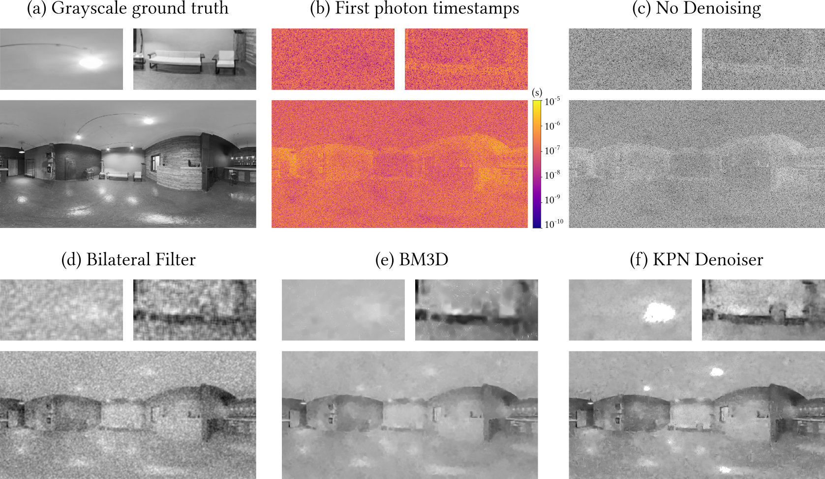
Supplementary Figure 4: Denoising IP-SPAD Images with Low Photon Counts: (a-b) We simulate the extreme case of IP-SPAD imaging by sampling at most one photon time stamp per pixel of a ground truth image. (c) Simply inverting the each time stamp is not enough due to extreme noise, (d-f) so it is necessary to combine time stamps spatially. (d) We apply a bilateral filter ($\sigma=7$), which incorporates some spatial information, but still remains quite noisy. (e) BM3D [14] may over smooth, and it seems to have particular trouble in bright regions. (f) Our KPN denoiser trained on photon timestamp data preserves some object shapes like the bright ceiling light and the couches.

Supplementary Note 3.3 Homoskedasticity of log-timestamps

In this section we show that the log-transformation is a variance stabilizing transformation for first-photon timestamp data. Let $Y\sim\text{Exp}(\Phi)$ be the arrival time of the first incident photon (we drop the subscript in $Y_{1}$ for simplicity). Our goal is to show that the variance of $\log(Y)$ is constant (homoskedasticity).

From the properties of the exponential distribution,

$$P(Y\leq t)= 1-e^{-\Phi t}$$ (S24)

$$\implies P(\log Y\leq\log t)= 1-e^{-\Phi t}.$$ (S25)

Defining $$\tilde{Y}=\log(Y) y=\log(t)$$ and ,

$$P(\tilde{Y}\leq y)= 1-e^{-\Phi e^{y}}$$ (S26)

$$\implies p_{\tilde{Y}}(y)= \Phi e^{-\Phi e^{y}}e^{y}$$ (S27)

where $$p_{\tilde{Y}}(y) \tilde{Y}$$ is the p.d.f. of .

$$\implies E[\tilde{Y}]= \int_{-\infty}^{\infty}y\Phi e^{-\Phi e^{y}}e^{y}\,dy$$ (S28)

$$= \int_{-\infty}^{\infty}\Phi ye^{y}e^{-\Phi e^{y}}\,dy.$$ (S29)

Take $$e^{y}=u$$

$$E[\tilde{Y}]= \int_{0}^{\infty}\Phi\log(u)e^{-\Phi u}\,du$$ (S30)

Take $$\Phi u=v$$

$$E[\tilde{Y}]= \int_{0}^{\infty}(\log(v)-\log(\Phi))e^{-v}dv$$ (S31)

$$= -\log(\Phi)+\int_{0}^{\infty}\log(v)e^{-v}dv$$ (S32)

$$= -\log(\Phi)-\gamma,$$ (S33)

where the second expression is an integral known to evaluate to $$-\gamma \gamma\approx 0.577 =\log(\nicefrac{{1}}{{\Phi}})$$ ( is the Euler-Mascheroni constant). We can see that the log-timestamp only has a constant bias away from the true log-timestamp (), which can be removed separately.

We repeat the same ideas for calculating the variance:

$$E[\tilde{Y}^{2}]= \int_{-\infty}^{\infty}y^{2}\Phi e^{-\Phi e^{y}}e^{y}\,dy$$ (S34)

Take $$e^{y}=u$$ again:

$$E[\tilde{Y}^{2}]= \int_{0}^{\infty}\Phi(\log^{2}u)e^{-\Phi u}\,du$$ (S35)

and $$v=\Phi u\implies\log u=\log v-\log\Phi$$. Then

$$E[\tilde{Y}^{2}]= \int_{0}^{\infty}\log^{2}(v)e^{-v}\,dv$$ (S36)

$$-2\log(\Phi)\int_{0}^{\infty}\log(v)e^{-v}\,dv$$

$$+\log^{2}(\Phi)$$

$$= \gamma^{2}+\nicefrac{{\pi^{2}}}{{6}}+2\gamma\log(\Phi)+\log^{2}(\Phi),$$ (S37)

where the first term on the right-hand side is also a known standard integral. Finally we have

$$\mathrm{Var}(\tilde{Y})= E[\tilde{Y}^{2}]-E[\tilde{Y}]^{2}=\nicefrac{{\pi^{2}}}{{6}},$$ (S38)

which proves the homoskedasticity of $\tilde{Y}=\log(Y)$.

Supplementary Note 4 Hardware Prototype

Our hardware prototype (5) consists of a single SPAD pixel mounted on two translation stages. Dead-time is controlled using a long cable that produces analog delay. After each photon detection event the SPAD pixel has to be kept disabled for few tens of $\mathrm{ns}\text{/}$ to lower the probability of afterpulses [12] and reset its original bias condition. Usually this dead-time is set either using the discharge time of an R-C network or employing a digital timing circuit, since the dead-time accuracy is not a limiting factor in conventional SPAD applications. In case of dead-time defined using digital timing circuits, there are implementations where its accuracy depends on the period of an uncorrelated (with respect to photon arrival times) digital clock. For example, a $100$ $\mathrm{MHz}\text{/}$ clock frequency will limit the accuracy of the dead-time to about $10$ $\mathrm{ns}\text{/}$, which is too coarse to get reliable photon flux estimates. This is true especially at extremely high photon flux values where photons get detected almost immediately after each dead-time duration ends. As described in the main text, we rely on low-jitter voltage comparators and analog delays introduced by long coaxial cables to obtain precisely controlled dead-time durations with low jitter.

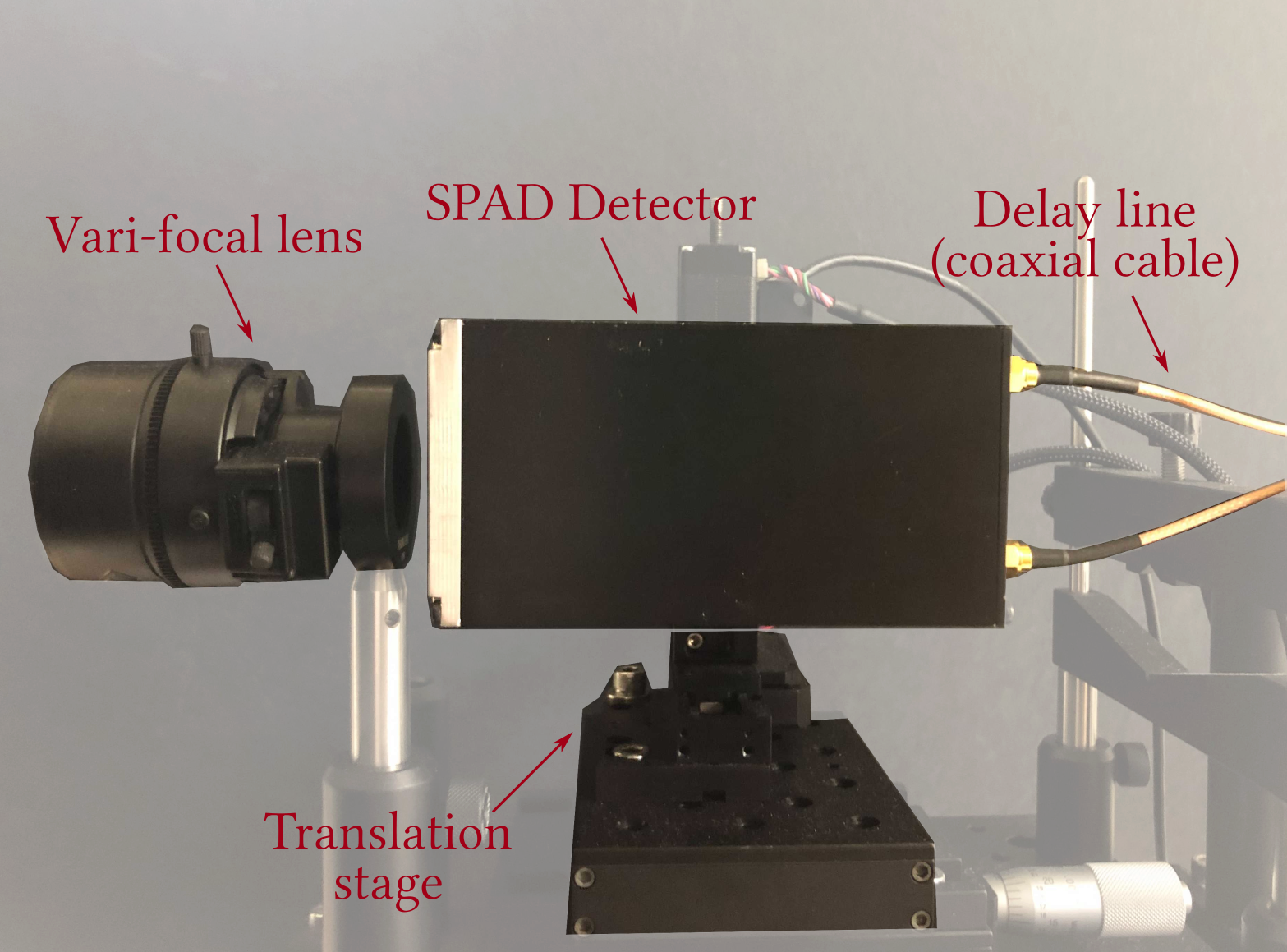
Supplementary Figure 5: The IP-SPAD hardware prototype consists of a single SPAD pixel mounted on translation stages to scan the image plane of a vari-focal lens (Fujinon DV3.4x3.8SA-1). Part of a $20\text{\,}\mathrm{m}\text{/}$ long co-axial cable used for generating the dead-time delay is also shown.

Supplementary Note 5 Pixel Non-idealities

When conducting experiments with our hardware prototype we found two non-idealities: dead-time drift and non-zero gate rise time.

Dead-time Drift

When imaging high flux regions for extended periods of time our hardware prototype’s dead-time increases; we call this dead-time drift. This is due to heating of the SPAD front-end. We calibrated each pixel position individually by constructing an inter-photon timing histogram and using the first non-zero bin of this histogram as an estimate of the true dead-time for that pixel position. Experimentally, we observed that the dead-time drift is slower than the 5ms exposure times used so this method should approximate the true dead-time well for each pixel position. Without this correction the error introduced by the drift dominates the denominator in Eq. (2) at high flux values, limiting the dynamic range.

Supplementary Figure 6: This figure shows inter-photon histograms for 4 points from the tunnel scene. Notice that the histograms are not aligned on the left edge, indicating a drift in dead-time. We correct for this drift by taking the time of the first non-zero bin as the dead-time for that pixel.

When our single-pixel IP-SPAD stays active for long periods of time dead-time drift becomes a problem. Suppl. Fig. 6 shows inter-photon timing histograms of four different scene points with increasing flux levels ($1\rightarrow 4$). Notice that the histograms are not aligned on the left edges indicating a difference in dead-times at these points. We correct for the dead-time drift in by using a dead-time estimate for each pixel in the final image. We set the dead-time estimate in a pixel to the smallest inter-arrival time from that pixel, this has the effect of shifting each pixel’s inter-arrival histogram to zero. In the tunnel scene the difference between the longest used and shortest used dead-time is $887\text{\,}\mathrm{ps}\text{/}$, a variation of about 0.8%.

Gate Rise Time

When the SPAD enters and exits the dead-time phase, its bias voltage has to be quickly changed from above to below the breakdown value, and vice-versa [8]. The duration of these transitions is as critical as the dead-time duration itself, and has to be short (in order to swiftly restore the SPAD bias for the next detection) and precise (to prevent variations in the overall dead-time duration). In our system the rise times are on the order of $200\text{\,}\mathrm{ps}\text{/}$: it translates into non-exponentially shaped inter-photon timing histograms, especially in high flux regions. We did not find that this behavior detrimentally effected our results; however, it has an effect similar to slightly tone mapping bright regions downward.

Unlike dead-time drift, the rise time behavior seems to be independent of how long the SPAD was exposed to a high flux source. Fig. 7 shows inter-photon timestamp histograms for increasing photon flux levels. Rise time causes these to deviate from an exponential shape at high flux levels.

We found that this behavior made it virtually impossible to fully saturate the SPAD pixel, that is increasing the incident flux would lead to a non-linear increase in photons counted. We performed an experiment where a laser was directly pointed into the SPAD active region and the power of the laser was increased. We found that the photon counts did not saturate before the SPAD overheated and shut itself off.

The rise-time behaviour can by incorporated into the flux estimator derived in Supplementary Note 1 using a time-varying quantum efficiency $q(t)$. For $t<0$, $q(t)=0$ and $\int_{0}^{\infty}q(t)dt\rightarrow\infty$. When the dead time ends, the IP-SPAD pixel’s $q(t)$ ramps up to its peak value. The probability distribution of time-of-darkness, $Y_{i}$, can be written as:

$$Y_{i}\sim f_{Y_{i}}(Y_{i}|Y_{1}\dots Y_{i-1})=\begin{cases}q(Y_{i})\Phi e^{-\Phi\int_{0}^{Y_{i}}q(l)dl}&\mbox{for }0<Y_{i}<T_{i}\\ e^{-\Phi\int_{0}^{T_{i}}q(l)dl}\,\cdot\,\delta(t-T_{i})&\mbox{for }Y_{i}=T_{i}\\ 0&\mbox{otherwise.}\end{cases}$$ (S39)

where $T_{i}$ is defined in Supplementary Note 1. For a series of $N$ timestamps with times-of-darkness given by $Y_{1}\dots Y_{N}$, we use a similar derivation to Supplementary Note 1 to find the maximum likelihood estimator (MLE):

$$\widehat{\Phi}=\frac{N}{\int^{T_{N+1}}_{0}q(t)dt+\sum_{i=1}^{N}\int^{Y_{i}}_{0}q(t)dt}.$$ (S40)

Eq. (S40) reduces to Eq. (S6) if $q(t)$ is an ideal step function. For the experimental results shown in the main text, the IP-SPAD pixel’s $q(t)$ was not precisely known so we could not apply this correction. Future work will look at estimating $q(t)$ from inter-photon histograms and quantifying SNR improvements from such a correction.

Supplementary Note 6 Additional Results

Supplementary Figure 7: Simulated Extreme Dynamic Range Scene: This figure shows simulated extreme dynamic range images using an IP-SPAD camera compared with a conventional camera with different exposure settings. (a) A $5\text{\,}\mathrm{ms}\text{/}$ exposure image with a conventional camera (full-well capacity 34,000 and read noise 5$e^{-}$ has many saturated pixels. Observe that the bright bulb region is washed out. (b) A short exposure image is dominated by shot noise in darker parts of the scene. It becomes visible only at a much lower exposure setting. Since this is a simulation we were able to reduce the exposure time down to $5\times 10^{-5}$ $\mathrm{ms}\text{/}$ which may be impossible to achieve with a conventional camera. In practice, this exposure can be achieved by, say, reducing the shutter speed to 1/16,000 and adding a 10-stop ND filter. (c) A PF-SPAD camera is able to capture both dark and bright regions in a single exposure, but the bright bulb filament still suffers from noise due to the soft-saturation phenomenon. (d) Our proposed IP-SPAD method estimates scene brightness using high-resolution timestamps to capture both extremely dark and extremely bright pixels, beyond the soft-saturation limit of a counts-based PF-SPAD. (Original image from HDRIHaven.com)

Supplementary Figure 8: Experimental Extreme Dynamic Range “Shelf” Scene: This “Shelf” scene shows extreme dynamic range, with a bright bulb filament in one of the shelves and text in the neighboring shelf which is dark and not directly illuminated by the light source. The bottom row of images uses a similar setup as the top row but also includes two bright LED lights in addition to the filament bulb. The conventional camera requires three exposures to cover the dynamic range of this scene. The proposed IP-SPAD flux estimator captures the scene in a single exposure.

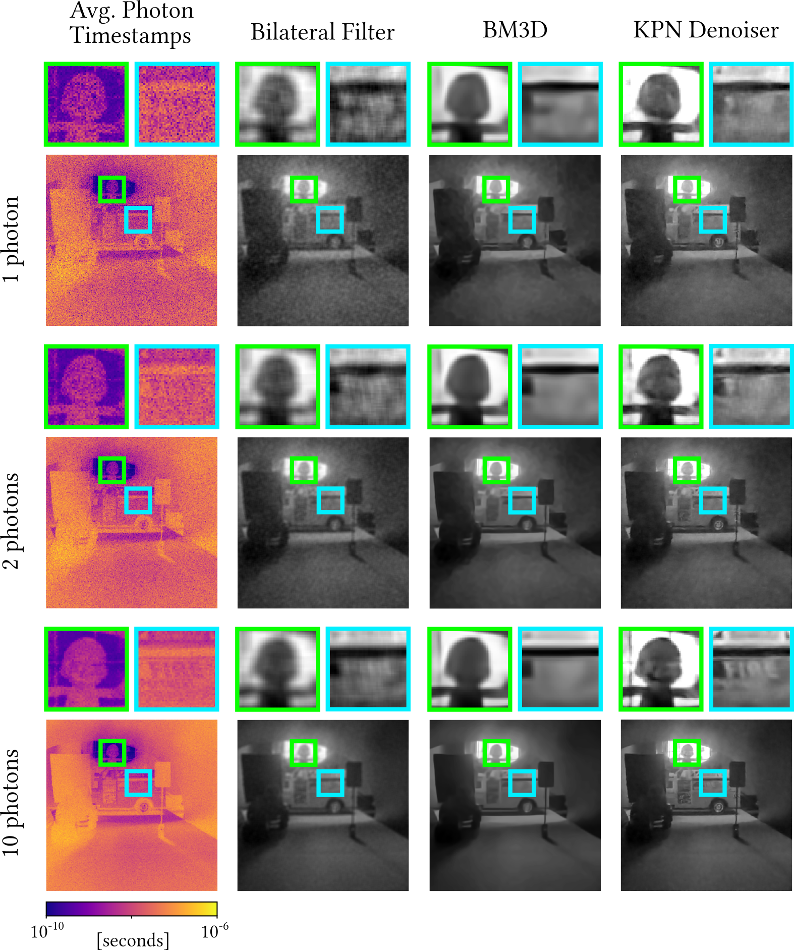
Supplementary Figure 9: Effect of Increasing Number of Photons on Denoising. Some image details start appearing with as few as 10 photon timestamps per pixel. For example, the text on the fire-truck is visible with images denoised with the bilateral filter and our KPN-based denoiser. BM3D appears to give less noisy results in this example but finer details are lost.

Supplementary Note 7 Pixel Designs for Passive SPAD Imaging

Supplementary Figure 10: IP-SPAD pixel designs for passive imaging: (a) and (b) are existing SPAD pixel designs with counts and in-pixel timing circuits. (c) and (d) are hypothetical future pixel designs for passive IP-SPAD cameras that store individual photon timestamps or compute summary statistics on the fly.

Passive SPAD Pixel Architectures Many current SPAD pixel designs are targeted towards specialized active imaging applications that operate the detector in synchronization with a light source, such as pulsed laser. The most common data processing task is to generate a timing histogram which counts the number of photons detected by the SPAD pixel as a function of the (discretized) time delay since the transmission of the most recent laser pulse. The requirements for the passive imaging technique shown in this paper are different: there is no pulsed light source to provide a timing reference. Instead, it is important to precisely control (1) the dead time duration (2) rise and fall times of the SPAD bias circuitry, and (3) the duration of the global exposure time.

Our single-pixel IP-SPAD hardware prototype, although acceptable as a proof-of-concept, is not a scalable solution for sensor arrays. Delay-locked loops circuits suitable for multi-pixel implementation can be used in the future to precisely control the dead-time duration. A large array of IP-SPAD pixels will generate an unreasonably large volume of raw photon timestamp data that cannot be transferred off the sensor chip for post-processing. A megapixel SPAD array has been recently demonstrated using a $180\text{\,}\mathrm{nm}\text{/}$ CMOS technology [39], but the in-pixel electronics is currently limited to gating circuitry and a 1-bit data register. The trade-off between SPAD performance and pixel number can be overcome by recently-developed 3D-stacking approaches where SPAD arrays are fabricated in a dedicated technology, the high density data-processing electronics are developed in scaled technology, and then the two chips/wafers are mounted one on top of the other [23, 10].

Fig. 10(a) shows the simplest single-pixel architecture currently used as a building-block in large SPAD arrays. It comprises the photodetector, its readout and quenching circuits and a digital counter, for storing the number of detected photons. While this architecture is widely used [6], it does not exploit photon arrival times to increase dynamic range. As shown in Fig. 10(b), adding an in-pixel time-to-digital converter (TDC) able to acquire and store individual photon time-stamps (with respect to the exposure time synchronization signal) can solve this limitation. Also this approach is nowadays quite common when designing SPAD arrays [24, 44], however, increasing the array dimension and considering a very high incident photon flux, it will be impractical to acquire and transfer timestamps for each photon and each pixel, because it will lead to intractable volume of data to be processed. Instead, a more efficient way of storing and transmitting photon time-stamp data for passive imaging can rely on simply storing the first and last photon time-stamps within a single exposure time, together with the total photon counts. The corresponding pixel design is shown in Fig. 10(c). While this increases pixel complexity over the previous SPAD pixel design examples, it only requires two additional data registers. The disadvantage of this scheme is that, depending on the total exposure time, the TDC may require a large full-scale range. For example, using an exposure time in the millisecond range and the timestamp resolution in picoseconds, the TDC data depth will be $\log_{2}(10^{-3}/10^{-12})\approx 30$ bits.

Note that our brightness estimator keeps track of the average time-of-darkness between photon detections over a fixed exposure time. An alternative to storing first and last timestamps may be to instead store a running average of the inter-photon times, as shown in Fig. 10(d). This can be implemented in-pixel using basic digital signal processing circuits. At high photon flux levels, the expected inter-photon times will be short enough that a TDC with smaller full scale range could be used. Although the inter-photon times may still be quite long for low flux levels, the flux estimator can fall back to using photon counts only, instead of timestamps.

SPAD Array Designs for Passive Imaging

The theoretical analysis and experimental results in this paper were restricted to a single SPAD pixel. For most passive imaging applications, in practice, there will be a need to scale this method to large form factor SPAD arrays with thousands of pixels. This will introduce additional design challenges and noise sources not discussed in this work. A large form-factor SPAD array of free-running SPAD pixels will generate an unreasonably large volume of raw photon time-stamp data that cannot be simply transferred off the sensor chip for post-processing. For instance, consider a hypothetical 1 megapixel SPAD array consisting of pixels shown in Fig. 10(b), with dead time of $100$ $\mathrm{ns}\text{/}$. Assume an average photon flux of ${10}^{5}$ photons/s over the pixel array and the pixels generate $32$-bit IEEE floating-point timestamps for each detected photon. This corresponds to $400$ $\mathrm{GiB}\text{/}\mathrm{s}$ of data generated from the chip. A megapixel SPAD array has been recently demonstrated using a 180nm CMOS technology [39] , but the in-pixel electronics is currently limited to gating circuitry and 1-bit data register (photon detected or not).

One possible solution to overcome this problem could include the design of large arrays using a combination of pixel architectures sketched in Fig. 10, i.e. where only a fraction of pixels would include high resolution TDCs while the rest of the pixels only use photon counters. This will still enable capturing extremely high flux values albeit with reduced spatial resolution. In another solution TDCs are shared among more pixels, while counters are integrated in each pixel. This will reduce the maximum count rate, but each detected photon is counted and time tagged.

SPAD performance (i.e. detection efficiency, dark count noise, temporal resolution, afterpulsing probability) in developing multi-pixel arrays is usually better when using “legacy” fabrication technologies, like 350 nm and 180 nm CMOS, or even “custom” technologies (which, however, do not allow the on-chip integration of ancillary electronics) [17]. With such technologies, the relatively large minimum feature size prevents in-pixel integration of sophisticated electronics like high-resolution (few $\mathrm{ps}\text{/}$) TDCs, data processing circuits and memories (unless without accepting an extremely low fill-factor). The trade-off between SPAD performance and pixel number can be overcome by recently-developed 3D-stacking approaches: SPAD array is fabricated in a dedicated technology, the high density data-processing electronics is developed in scaled technology, and then the two chips/wafers are mounted one on top of the other [23, 10].

Passive IP-SPAD arrays may also require pixel-wise calibration. The non-linear pixel response curve may make this more challenging than conventional CMOS camera pixels. It will be necessary to characterize non-uniformity in terms of dead-time durations and timing jitter and account for these for removing any fixed pattern noise.

Another important practical consideration is power requirement, especially when operating in high flux conditions where a large number of avalanches will be created causing huge power requirement for processing these in real-time and reading out the counts. There is also a significant heat dissipation issue which can exacerbate pixel calibration due to the strong temperature dependence of various pixel parameters like dark count rate and dead-time drifts. Such power issues may be mitigated with scaled technologies operating at lower supply voltage.

References

- [1] U.S. Department of Energy (Disclaimer): This work was prepared as an account of work sponsored by an agency of the United States Government. Neither the United States Government nor any agency thereof, nor any of their employees, nor any of their contractors, subcontractors or their employees, makes any warranty, express or implied, or assumes any legal liability or responsibility for the accuracy, completeness, or any third party’s use or the results of such use of any information, apparatus, product, or process disclosed, or represents that its use would not infringe privately owned rights. Reference herein to any specific commercial product, process, or service by trade name, trademark, manufacturer, or otherwise, does not necessarily constitute or imply its endorsement, recommendation, or favoring by the United States Government or any agency thereof or its contractors or subcontractors. The views and opinions of authors expressed herein do not necessarily state or reflect those of the United States Government or any agency thereof, its contractors or subcontractors.
- [2] Eirikur Agustsson and Radu Timofte. Ntire 2017 challenge on single image super-resolution: Dataset and study. In The IEEE Conference on Computer Vision and Pattern Recognition (CVPR) Workshops, July 2017.
- [3] F J Anscombe. The Transformation of Poisson, Binomial and Negative-Binomial Data. Biometrika, 35(3-4):246 – 254, Dec. 1948.
- [4] Ivan Michel Antolovic, Claudio Bruschini, and Edoardo Charbon. Dynamic range extension for photon counting arrays. Optics Express, 26(17):22234, aug 2018.
- [5] Steve Bako, Thijs Vogels, Brian Mcwilliams, Mark Meyer, Jan Novák, Alex Harvill, Pradeep Sen, Tony Derose, and Fabrice Rousselle. Kernel-predicting convolutional networks for denoising monte carlo renderings. ACM Trans. Graph., 36(4), July 2017.
- [6] Danilo Bronzi, Federica Villa, Simone Tisa, Alberto Tosi, and Franco Zappa. Spad figures of merit for photon-counting, photon-timing, and imaging applications: a review. IEEE Sensors Journal, 16(1):3–12, 2015.
- [7] Claudio Bruschini, Harald Homulle, Ivan Michel Antolovic, Samuel Burri, and Edoardo Charbon. Single-photon avalanche diode imagers in biophotonics: review and outlook. Light: Science & Applications, 8(1):1–28, 2019.
- [8] Mauro Buttafava, Gianluca Boso, Alessandro Ruggeri, Alberto Dalla Mora, and Alberto Tosi. Time-gated single-photon detection module with 110 ps transition time and up to 80 mhz repetition rate. Review of Scientific Instruments, 85(8):083114, 2014.
- [9] Mauro Buttafava, Jessica Zeman, Alberto Tosi, Kevin Eliceiri, and Andreas Velten. Non-line-of-sight imaging using a time-gated single photon avalanche diode. Optics express, 23(16):20997–21011, 2015.
- [10] Edoardo Charbon, Claudio Bruschini, and Myung-Jae Lee. 3d-stacked CMOS SPAD image sensors: Technology and applications. In 2018 25th IEEE International Conference on Electronics, Circuits and Systems (ICECS). IEEE, dec 2018.
- [11] Sergio Cova, Massimo Ghioni, Andrea Lacaita, Carlo Samori, and Franco Zappa. Avalanche photodiodes and quenching circuits for single-photon detection. Applied optics, 35(12):1956–1976, 1996.
- [12] S. Cova, A. Lacaita, and G. Ripamonti. Trapping phenomena in avalanche photodiodes on nanosecond scale. IEEE Electron Device Letters, 12(12):685–687, 1991.
- [13] Eugenio Culurciello, Ralph Etienne-Cummings, and Kwabena A Boahen. A biomorphic digital image sensor. IEEE Journal of Solid-State Circuits, 38(2):281–294, 2003.
- [14] Kostadin Dabov, Alessandro Foi, Vladimir Katkovnik, and Karen Egiazarian. Image denoising with block-matching and 3d filtering. Proceedings of SPIE - The International Society for Optical Engineering, 6064:354–365, 02 2006.
- [15] Kostadin Dabov, Alessandro Foi, Vladimir Katkovnik, and Karen Egiazarian. Image denoising by sparse 3-d transform-domain collaborative filtering. IEEE Transactions on image processing, 16(8):2080–2095, 2007.
- [16] Neale AW Dutton, Tarek Al Abbas, Istvan Gyongy, Francescopaolo Mattioli Della Rocca, and Robert K Henderson. High dynamic range imaging at the quantum limit with single photon avalanche diode-based image sensors. Sensors, 18(4):1166, 2018.
- [17] M. Ghioni, A. Gulinatti, I. Rech, F. Zappa, and S. Cova. Progress in silicon single-photon avalanche diodes. IEEE Journal of Selected Topics in Quantum Electronics, 13(4):852–862, 2007.
- [18] Abhiram Gnanasambandam, Omar Elgendy, Jiaju Ma, and Stanley H Chan. Megapixel photon-counting color imaging using quanta image sensor. Optics express, 27(12):17298–17310, 2019.
- [19] Javier Grau Chopite, Matthias B Hullin, Michael Wand, and Julian Iseringhausen. Deep non-line-of-sight reconstruction. arXiv, pages arXiv–2001, 2020.
- [20] Anant Gupta, Atul Ingle, and Mohit Gupta. Asynchronous single-photon 3d imaging. In Proceedings of the IEEE International Conference on Computer Vision, pages 7909–7918, 2019.
- [21] Mohit Gupta, Daisuke Iso, and Shree K. Nayar. Fibonacci exposure bracketing for high dynamic range imaging. In 2013 IEEE International Conference on Computer Vision. IEEE, dec 2013.
- [22] S. W. Hasinoff, F. Durand, and W. T. Freeman. Noise-optimal capture for high dynamic range photography. In 2010 IEEE Computer Society Conference on Computer Vision and Pattern Recognition, pages 553–560, June 2010.
- [23] Robert K. Henderson, Nick Johnston, Sam W. Hutchings, Istvan Gyongy, Tarek Al Abbas, Neale Dutton, Max Tyler, Susan Chan, and Jonathan Leach. 5.7 a 256×256 40nm/90nm CMOS 3d-stacked 120db dynamic-range reconfigurable time-resolved SPAD imager. In 2019 IEEE International Solid- State Circuits Conference - (ISSCC). IEEE, feb 2019.
- [24] Robert K. Henderson, Nick Johnston, Francescopaolo Mattioli Della Rocca, Haochang Chen, David Day-Uei Li, Graham Hungerford, Richard Hirsch, David Mcloskey, Philip Yip, and David J. S. Birch. A 192x128 time correlated SPAD image sensor in 40-nm CMOS technology. IEEE Journal of Solid-State Circuits, 54(7):1907–1916, jul 2019.
- [25] Atul Ingle, Andreas Velten, and Mohit Gupta. High flux passive imaging with single-photon sensors. In Proceedings of the IEEE Conference on Computer Vision and Pattern Recognition, pages 6760–6769, 2019.
- [26] Steven D. Johnson, Paul-Antoine Moreau, Thomas Gregory, and Miles J. Padgett. How many photons does it take to form an image? Applied Physics Letters, 116(26):260504, jun 2020.
- [27] Spyros Kavadias, Bart Dierickx, Danny Scheffer, Andre Alaerts, Dirk Uwaerts, and Jan Bogaerts. A logarithmic response cmos image sensor with on-chip calibration. IEEE Journal of Solid-state circuits, 35(8):1146–1152, 2000.
- [28] Diederik P. Kingma and Jimmy Ba. Adam: A method for stochastic optimization, 2017.
- [29] Ahmed Kirmani, Tyler Hutchison, James Davis, and Ramesh Raskar. Looking around the corner using transient imaging. In 2009 IEEE 12th International Conference on Computer Vision, pages 159–166. IEEE, 2009.
- [30] Ahmed Kirmani, Dheera Venkatraman, Dongeek Shin, Andrea Colaço, Franco N. C. Wong, Jeffrey H. Shapiro, and Vivek K Goyal. First-photon imaging. Science, 343(6166):58–61, nov 2013.
- [31] Martin Laurenzis. Single photon range, intensity and photon flux imaging with kilohertz frame rate and high dynamic range. Optics Express, 27(26):38391, dec 2019.
- [32] Timothy Lee. Most lidars today have between 1 and 128 lasers—this one has 11,000. Ars Technica, Jan 2020. Accessed Nov 16, 2020.
- [33] David B Lindell and Gordon Wetzstein. Three-dimensional imaging through scattering media based on confocal diffuse tomography. Nature communications, 11(1):1–8, 2020.
- [34] Scott Lindner, Chao Zhang, Ivan Michel Antolovic, Martin Wolf, and Edoardo Charbon. A 252 x 144 spad pixel flash lidar with 1728 dual-clock 48.8 ps tdcs, integrated histogramming and 14.9-to-1 compression in 180nm cmos technology. In 2018 IEEE Symposium on VLSI Circuits, pages 69–70. IEEE, 2018.
- [35] Xiaochun Liu, Ibón Guillén, Marco La Manna, Ji Hyun Nam, Syed Azer Reza, Toan Huu Le, Adrian Jarabo, Diego Gutierrez, and Andreas Velten. Non-line-of-sight imaging using phasor-field virtual wave optics. Nature, 572(7771):620–623, 2019.
- [36] Sizhuo Ma, Shantanu Gupta, Arin C Ulku, Claudio Bruschini, Edoardo Charbon, and Mohit Gupta. Quanta burst photography. ACM Transactions on Graphics (TOG), 39(4):79–1, 2020.
- [37] Raffi Mardirosian. Why Apple chose digital lidar. Ouster Blog, Apr 2020. Accessed Nov 16, 2020.
- [38] Ben Mildenhall, Jonathan T Barron, Jiawen Chen, Dillon Sharlet, Ren Ng, and Robert Carroll. Burst denoising with kernel prediction networks. In IEEE Conference on Computer Vision and Pattern Recognition (CVPR), 2018.
- [39] Kazuhiro Morimoto, Andrei Ardelean, Ming-Lo Wu, Arin Can Ulku, Ivan Michel Antolovic, Claudio Bruschini, and Edoardo Charbon. Megapixel time-gated SPAD image sensor for 2d and 3d imaging applications. Optica, 7(4):346, apr 2020.
- [40] S.K. Nayar and T. Mitsunaga. High dynamic range imaging: spatially varying pixel exposures. In Proceedings IEEE Conference on Computer Vision and Pattern Recognition. CVPR 2000 (Cat. No.PR00662). IEEE Comput. Soc, 2000.
- [41] Matthew O’Toole, Felix Heide, David B Lindell, Kai Zang, Steven Diamond, and Gordon Wetzstein. Reconstructing transient images from single-photon sensors. In Proceedings of the IEEE Conference on Computer Vision and Pattern Recognition, pages 1539–1547, 2017.
- [42] Sylvain Paris. A gentle introduction to bilateral filtering and its applications. In ACM SIGGRAPH 2007 courses, pages 3–es. 2007.
- [43] Matteo Perenzoni, Nicola Massari, Daniele Perenzoni, Leonardo Gasparini, and David Stoppa. A 160 x 120 pixel analog-counting single-photon imager with time-gating and self-referenced column-parallel a/d conversion for fluorescence lifetime imaging. IEEE Journal of Solid-State Circuits, 51(1):155–167, 2015.
- [44] Davide Portaluppi, Enrico Conca, and Federica Villa. 32 × 32 CMOS SPAD imager for gated imaging, photon timing, and photon coincidence. IEEE Journal of Selected Topics in Quantum Electronics, 24(2):1–6, mar 2018.
- [45] Joshua Rapp, Yanting Ma, Robin MA Dawson, and Vivek K Goyal. Dead time compensation for high-flux ranging. IEEE Transactions on Signal Processing, 67(13):3471–3486, 2019.
- [46] Joshua Rapp, Yanting Ma, Robin MA Dawson, and Vivek K Goyal. High-flux single-photon lidar. Optica, 8(1):30–39, 2021.
- [47] Joshua Rapp, Julian Tachella, Yoann Altmann, Stephen McLaughlin, and Vivek K Goyal. Advances in single-photon lidar for autonomous vehicles: Working principles, challenges, and recent advances. IEEE Signal Processing Magazine, 37(4):62–71, 2020.
- [48] Julián Tachella, Yoann Altmann, Nicolas Mellado, Aongus McCarthy, Rachael Tobin, Gerald S Buller, Jean-Yves Tourneret, and Stephen McLaughlin. Real-time 3D reconstruction from single-photon lidar data using plug-and-play point cloud denoisers. Nature communications, 10(1):1–6, 2019.
- [49] The ImageMagick Development Team. Imagemagick.
- [50] Radu Timofte, Eirikur Agustsson, Luc Van Gool, Ming-Hsuan Yang, Lei Zhang, Bee Lim, et al. Ntire 2017 challenge on single image super-resolution: Methods and results. In The IEEE Conference on Computer Vision and Pattern Recognition (CVPR) Workshops, July 2017.
- [51] Alex Turpin, Gabriella Musarra, Valentin Kapitany, Francesco Tonolini, Ashley Lyons, Ilya Starshynov, Federica Villa, Enrico Conca, Francesco Fioranelli, Roderick Murray-Smith, et al. Spatial images from temporal data. Optica, 7(8):900–905, 2020.
- [52] Arin Can Ulku, Claudio Bruschini, Ivan Michel Antolovic, Yung Kuo, Rinat Ankri, Shimon Weiss, Xavier Michalet, and Edoardo Charbon. A 512x512 spad image sensor with integrated gating for widefield flim. IEEE Journal of Selected Topics in Quantum Electronics, 25(1):1–12, jan 2019.
- [53] Feng Yang, Yue M Lu, Luciano Sbaiz, and Martin Vetterli. Bits from photons: Oversampled image acquisition using binary poisson statistics. IEEE Transactions on image processing, 21(4):1421–1436, 2011.
- [54] Junko Yoshida. Breaking Down iPad Pro 11’s LiDAR Scanner. EE Times, Jun 2020. Accessed Nov 16, 2020.
- [55] Majid Zarghami, Leonardo Gasparini, Matteo Perenzoni, and Lucio Pancheri. High dynamic range imaging with TDC-based CMOS SPAD arrays. Instruments, 3(3):38, aug 2019.
- [56] Hang Zhao, Boxin Shi, Christy Fernandez-Cull, Sai-Kit Yeung, and Ramesh Raskar. Unbounded high dynamic range photography using a modulo camera. In 2015 IEEE International Conference on Computational Photography (ICCP), pages 1–10. IEEE, 2015.
Supplementary Document for