Geometric properties of a domain with cusps

Abstract.

For $n\geq 4$ (even), the function $\varphi_{n\mathcal{L}}(z)=1+nz/(n+1)+z^{n}/(n+1)$ maps the unit disk $\mathbb{D}$ onto a domain bounded by an epicycloid with $n-1$ cusps. In this paper, the class $\mathcal{S}^{*}_{n\mathcal{L}}=\mathcal{S}^{*}(\varphi_{n\mathcal{L}})$ is studied and various inclusion relations are established with other subclasses of starlike functions. The bounds on initial coefficients is also computed. Various radii problems are also solved for the class $\mathcal{S}^{*}_{n\mathcal{L}}.$

1. Introduction

An Epicycloid[12] is a plane curve produced by tracing the path of a chosen point on the circumference of a circle of radius $b$ which rolls without slipping around a fixed circle of radius $a$. The parametric equation of an epicycloid is

$$x(t) =m\cos t-b\cos\left(\frac{mt}{b}\right),$$

$$y(t) =m\sin t-b\sin\left(\frac{mt}{b}\right),\qquad-\pi\leq t\leq\pi,$$

where $m=a+b.$ If $m/b$ is an integer, then the curve has $m/b-1$ cusps. Some of the epicycloid have special names. For $a=b,$ the curve obtained is called a cardiod and has one cusp; for $a=2b$ it is a nephroid with two cusps and for $a=5b$, the curve formed is called ranunculoid, a five-cusped epicycloid. A parametric curve $\left(f(t),g(t)\right)$ has a cusp [6] at the point $\left(f(t_{0}),g(t_{0})\right)$ if $f^{\prime}(t_{0})$ and $g^{\prime}(t_{0})$ is zero but either $f^{\prime\prime}(t_{0})$ or $g^{\prime\prime}(t_{0})$ is not equal to zero. Many curves have been widely studied having no cusp, one cusp, two cusps and three cusps. For instance, the boundary of image domains of the functions $e^{z}$, $1+\sin z$ and $2/(1+e^{-z})$[2, 4, 19], under unit disk, have no cusp. The Lemniscate of Bernoulli $\sqrt{1+z}$, the reverse Lemniscate $\varphi_{RL}(z)$ and cardiod type domain (see[5, 11, 18, 24, 26, 28]) contains one cusp on the real axis. Nephroid [31] has two cusps on real axis whereas lune[22] and petal-like domain [27] contains two cusps at the angle $\pi/2$ and $3\pi/2.$ Gandhi [3] studied the class of functions for which boundary of the image domain contains three cusps, one on real axis and two at the angles $\pi/3$ and $5\pi/3.$ Motivated by this work, we have considered a more general domain whose boundary has the following parametric form:

(1.1) $$\begin{split}x(t)&=1+\frac{n}{n+1}\cos t+\frac{1}{n+1}\cos(nt),\\ y(t)&=\frac{n}{n+1}\sin t+\frac{1}{n+1}\sin(nt),\end{split}$$

for $n\geq 4$ (even). For $a=(n-1)/(n+1)$ and $b=1/(n-1),$ the curve (1.1) represents a rotated and translated epicycloid[17] with $(n-1)$ cusps. It is an algebraic curve of order $2n$. It can be easily seen that $x^{\prime}(t_{k})=0$ and $y^{\prime}(t_{k})=0$ for $t_{k}=(2k-1)\pi/(n-1),$ where $k=1,2,\ldots(n-2)/2.$ Also, $x^{\prime\prime}(t_{k})$ and $y^{\prime\prime}(t_{k})$ are not zero together. By the definition of cusps, the curve (1.1) has cusps at the points $t_{k}.$ The function $\varphi_{n\mathcal{L}}:\mathbb{D}\rightarrow\mathbb{C}$ given by

(1.2) $$\varphi_{n\mathcal{L}}(z)=1+\frac{nz}{n+1}+\frac{z^{n}}{n+1},\quad(z\in\mathbb{D})$$

maps unit circle to this curve and the unit disk onto the region bounded by the curve (1.1).

Ma and Minda[13] introduced the unified class of starlike functions $\mathcal{S}^{*}(\varphi)$ consisting of functions $f\in\mathcal{S}$ such that $zf^{\prime}(z)/f(z)\prec\varphi(z),$ for all $z\in\mathbb{D},$ where $\varphi$ is univalent function having positive real part, $\varphi(\mathbb{D})$ is symmetric about real axis and starlike with respect to $\varphi(0)=1$ and $\varphi^{\prime}(0)>0.$ The image domain $\varphi_{n\mathcal{L}}(\mathbb{D})$ is symmetric about real axis, has positive real part and starlike with respect to $\varphi_{n\mathcal{L}}(0)=1$. Also, $\varphi_{n\mathcal{L}}^{\prime}(0)>0.$ Thus, the function satisfies all the conditions of Ma-Minda class and hence we can define the following class.

Let $\mathcal{S}^{*}_{n\mathcal{L}}=\mathcal{S}^{*}(\varphi_{n\mathcal{L}})$ be the class of function $f:\mathbb{D}\rightarrow\mathbb{C}$ such that

$$\frac{zf^{\prime}(z)}{f(z)}\prec\varphi_{n\mathcal{L}}(z)=1+\frac{nz}{n+1}+\frac{z^{n}}{n+1},\quad(z\in\mathbb{D}),$$

for $n\geq 4,$ even. A function $f:\mathbb{D}\rightarrow\mathbb{C}$ belongs to the class $\mathcal{S}^{*}_{n\mathcal{L}}$ if and only if there exists an analytic function $\phi$ satisfying $\phi\prec\varphi_{n\mathcal{L}}$ such that

$$f(z)=z\exp\left(\int_{0}^{z}\frac{\phi(t)-1}{t}dt\right)$$

The function $f_{n\mathcal{L}}:\mathbb{D}\rightarrow\mathbb{C}$ given by

(1.3) $$f_{n\mathcal{L}}(z)=z\exp\left(\frac{n}{n+1}z+\frac{1}{n(n+1)}z^{n}\right)=z+\frac{n}{n+1}z^{2}+\frac{n^{2}}{2(n+1)}z^{3}+\ldots,$$

where $\varphi_{n\mathcal{L}}$ is given by (1.2). This function acts as extremal function for most of the results for the class $\mathcal{S}^{*}_{n\mathcal{L}}.$ Also, the concept of cusps is important to study the geometry for this domain as the cusp at the angle $\pi/(n-1)$ plays a vital role in computing various radii constants concerning the class $\mathcal{S}^{*}_{n\mathcal{L}}.$ Also, the class $\mathcal{S}^{*}_{n\mathcal{L}}$ becomes the class $\mathcal{S}^{*}(1+z)$ as the limit $n\rightarrow\infty.$ In the limiting case, the $n$-cusp domain transforms to the disk with center and radius $1$ (see Figure 1).

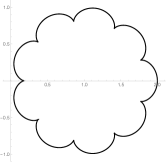
(a) n=10

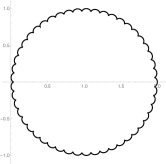
(b) n=50

(c) n=100

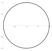
(d) n=1000

Figure 1. Limiting case

In the present work, various inclusion relations and radii problems for the class $\mathcal{S}^{*}_{n\mathcal{L}}$ are investigated. The sharp bounds for the first fifth coefficients of a function $f\in\mathcal{S}^{*}_{n\mathcal{L}}$ are computed. Further, various inclusion relations have been established between the class $\mathcal{S}^{*}_{n\mathcal{L}}$ and various subclasses of starlike functions such as $\mathcal{S}^{*}(\alpha),\,\mathcal{S}\mathcal{S}^{*}(\beta)$ and many others. Also, the sharp $\mathcal{S}^{*}_{n\mathcal{L}}-$radius is computed for various known classes os starlike functions and radius estimates for the class $\mathcal{S}^{*}(1+z)$ are obtained by taking the limit as $n\rightarrow\infty.$ In the last section, the radii constants for the class $\mathcal{S}^{*}_{n\mathcal{L}}$ are computed.

Lemma 1.1.

For $(n+1)<a<2,$ let $r_{a}$ be given by

$$r_{a}=\begin{cases}a-\displaystyle\frac{2}{n+1},&\displaystyle\frac{2}{n+1}<a\leq 1,\\ \sigma\left(\displaystyle\frac{\pi}{n-1}\right),&1\leq a<a_{3},\\ 2-a,&a_{3}<a<2,\end{cases}$$

where $a_{3}$ is the solution of the equation $\displaystyle\sigma\left(\pi/(n-1)\right)=\sigma(0)$ and the function $\sigma$ is the square of the distance from the point $(a,0)$ to the points on the curve $\partial\varphi_{n\mathcal{L}}(\mathbb{D}).$ Then $\{w:|w-a|<r_{a}\}\subseteq\varphi_{n\mathcal{L}}(\mathbb{D})$.

Proof.

Let $\varphi_{n\mathcal{L}}(z)$ be given by (1.2). Then any point on the boundary of $\varphi_{n\mathcal{L}}(\mathbb{D})$ is of the form $\varphi_{n\mathcal{L}}(e^{it})$. Since the curve $w=\varphi_{n\mathcal{L}}(e^{it})$ is symmetric with respect to real axis, so it is sufficient to consider the interval $0\leq t\leq\pi$. The parametric equation of $\varphi_{n\mathcal{L}}(e^{it})$ is given as follows:

$$\varphi_{n\mathcal{L}}(e^{it})=1+\frac{n}{n+1}\cos t+\frac{1}{n+1}\cos(nt)+i\left(\frac{n}{n+1}\sin t+\frac{1}{n+1}\sin(nt)\right)\\$$

The square of the distance from the point $(a,0)$ to the points on the curve $\varphi_{n\mathcal{L}}(e^{it})$ is given by:

(1.4) $$\sigma(t)=\left(1+\frac{n}{n+1}\cos t+\frac{1}{n+1}\cos(nt)-a\right)^{2}+\left(\frac{n}{n+1}\sin t+\frac{1}{n+1}\sin(nt)\right)^{2}.$$

It can be easily seen that

$$\sigma^{\prime}(t)=4n\cos\left(\frac{(n-1)t}{2}\right)\left[(n-1)\sin\left(\frac{(1-n)t}{2}\right)+(n+1)(a-1)\sin\left(\frac{(1+n)t}{2}\right)\right].$$

A calculation shows that $\sigma^{\prime}(t)=0$ for $t=0,\pi,\frac{\pi}{n-1},\frac{3\pi}{n-1},\cdots,\frac{(n-3)}{n-1}\pi$ and

$$\sigma^{\prime\prime}(t)=\frac{-2n\left((1-a)(1+n)\cos t+(1-a)n(n+1)\cos(nt)+(n-1)^{2}\cos(t-nt)\right)}{(n+1)^{2}}.$$

Clearly, it can be seen that

$$\sigma^{\prime\prime}(0)=\displaystyle\frac{2n(a(1+n)^{2}-2(1+n^{2}))}{(1+n)^{2}}>0,\text{ for }a>\frac{2(1+n^{2})}{(1+n)^{2}}>1.$$

Also, $\sigma^{\prime\prime}(\pi)>0$ for $a>2/(1+n)$ and

$$\sigma^{\prime\prime}\left(\frac{\pi}{n-1}\right)>0\text{ for }a<a_{1}=1-\frac{(n-1)^{2}}{(1+n)\cos\left(\frac{\pi}{n-1}\right)+n(n+1)\cos\left(\frac{n\pi}{n-1}\right)},$$

and $a_{1}>2(1+n^{2})/(1+n)^{2}>1.$ Let us assume $a<1.$ Now, $\sigma(\frac{\pi}{n-1})-\sigma(\pi)>0$ yields $(-1+a)(1+n)(-1+n+n\cos(\pi/(n-1))+\cos(n\pi/(n-1)))<0$. Also, $(-1+n+n\cos(\pi/(n-1))+\cos(n\pi/(n-1))>0$ and therefore $\sigma(\pi/(n-1))-\sigma(\pi)>0$. Hence, minimum value cannot be $\sigma(\pi/n-1)$. Consider $\sigma(k\pi/(n-1))-\sigma(\pi)=(-1+a)(1+n)(-1+n+n\ cos(k\pi/(n-1))+\cos(kn\pi/(n-1)))>0,$ for $k=3,5,\dots,n-3.$ Since $(-1+n+n\cos(k\pi/(n-1))+\cos(kn\pi/(n-1)))>0,$ $\sigma(k\pi/(n-1))$ cannot be minimum for this case. By checking the sign of second derivative, minimum can be $\sigma(\pi/(n-1))$, $\sigma(k\pi/(n-1))$ or $\sigma(\pi)$ where $k=3,5,\dots,n-3$. A simple computation gives $\sigma(k\pi/(n-1))-\sigma(\pi)>0$ and $\sigma(\pi/(n-1))-\sigma(\pi)>0$ and therefore minimum is $\sigma(\pi)$.

Let us assume $a>1.$ For this case, $\sigma(\pi)>\sigma(\pi/(n-1))$ and thus $\sigma(\pi)$ cannot be minimum and $\sigma(0)$ can be minima for $a>2(1+n^{2})/(1+n)^{2}$. In the interval $(1,2(1+n^{2})/(1+n)^{2})$ minimum can be $\sigma(\pi/(n-1))$ or $\sigma(k\pi/(n-1))$. By considering $\sigma(k\pi/(n-1))-\sigma(\pi/(n-1))=(a-1)(n(\cos(\pi/(n-1))-\cos(k\pi/(n-1))+(\cos(n\pi/(n-1)-\cos(kn\pi/(n-1))$ which can be proved to be greater than $0$ for $a>1$ and therefore $\sigma(k\pi/(n-1))$ cannot be the minimum and hence in the interval $(1,2(1+n^{2})/(1+n)^{2})$ minimum is $\sigma(\pi/(n-1))$. Now, we discuss the minimum in the interval $(2(1+n^{2})/(1+n)^{2},a_{1})$. A calculation shows that $\sigma\left(\pi/(n-1)\right)-\sigma(0)>0$ for

$$a>a_{3}=\frac{-(1+4n+n^{2})+n(1+n)\cos\left(\frac{\pi}{n-1}\right)+(n+1)\cos\left(\frac{n\pi}{n-1}\right)}{n(1+n)\cos\left(\frac{\pi}{n-1}\right)+(n+1)\cos\left(\frac{n\pi}{n-1}\right)-(n+1)^{2}},$$

which is also the solution of the equation $\displaystyle\sigma\left(\pi/(n-1)\right)=\sigma(0)$. Also, $a_{3}$ belongs to the interval $(2(1+n^{2})/(1+n)^{2},a_{1})$. Hence, $\sigma(\pi/(n-1))$ is minimum for $(2(1+n^{2})/(1+n)^{2},a_{3})$ and $\sigma(0)$ is minimum for $(a_{3},2)$. ∎

2. Coefficient Estimates

In this section, we will compute bounds on the coefficients for function in class $\mathcal{S}^{*}_{n\mathcal{L}}.$ The proof will use the following estimates (see [9], [21], [23], respectively) for the class of analytic functions $p(z)=1+c_{1}z+c_{2}z^{2}+\cdots$ such that $\operatorname{Re}p(z)>0$ for all $z\in\mathbb{D}.$

Lemma 2.1.

For $p(z)=1+c_{1}z+c_{2}z^{2}+\cdots\in\mathcal{P},$ then the following estimates holds.

• $|c_{2}-vc_{1}^{2}|\leq 2\max\{1,|2v-1|\},$

• $|c_{3}-2\beta c_{1}c_{3}+\delta c_{1}^{3}|\leq 2$ if $0\leq\beta\leq 1$ and $\beta(2\beta-1)\leq\delta\leq\beta,$

• $|\gamma c_{1}^{4}+ac_{2}^{2}+2\alpha c_{1}c_{3}-(3/2)\beta c_{1}^{2}c_{2}-c_{4}|\leq 2,$ when $0<\alpha<1,\,0<a<1$ and $8a(1-a)((\alpha\beta-2\gamma)^{2}+(\alpha(a+\alpha)-\beta)^{2})+\alpha(1-\alpha)(\beta-a\alpha)^{2}\leq 4\alpha^{2}(1-\alpha)^{2}a(1-a).$

Theorem 2.2.

If $f(z)=z+a_{2}z^{2}+a_{3}z^{3}+\cdots\in\mathcal{S}^{*}_{n\mathcal{L}},$ then $|a_{2}|\leq n/(n+1),\,|a_{3}|\leq n/(2(n+1)),\,|a_{4}|\leq n/(12(n+1))$ and $|a_{5}|\leq n/(4(n+1)).$ All the estimates are best possible.

Proof.

Let $p(z)=zf^{\prime}(z)/f(z)=1+b_{1}z+b_{2}z^{2}+\cdots\in\mathcal{P}.$ A simple computation gives

(2.1) $$(n-1)a_{n}=\sum_{k=1}^{n-1}b_{k}a_{n-k},\,\text{for }n>1.$$

Since $\varphi_{n\mathcal{L}}$ is univalent and $p\prec\varphi_{n\mathcal{L}}$, we get

$$p_{1}(z)=\frac{1+\varphi^{-1}_{n\mathcal{L}}\left(p(z)\right)}{1-\varphi^{-1}_{n\mathcal{L}}\left(p(z)\right)}=1+c_{1}z+c_{2}z^{2}+c_{3}z^{3}\cdots\in\mathcal{P}.$$

Thus,

$$p(z)=\varphi_{n\mathcal{L}}\left(\frac{p_{1}(z)-1}{p_{1}(z)+1}\right).$$

A calculation using (2.1) gives

$$a_{2} =b_{1}=\frac{n}{2(n+1)}c_{1}$$

$$a_{3} =\frac{n}{8(n+1)^{2}}\left(16\left(n+1\right)c_{2}-c_{1}^{2}\right)$$

$$a_{4} =\frac{n}{48(n+1)^{3}}\left(\left(n+2\right)c_{1}^{3}-2\left(n^{2}+5n+4\right)c_{1}c_{2}+8\left(n^{2}+2n+1\right)c_{3}\right)$$

$$a_{5} =\frac{n}{384}\left(\frac{48}{n+1}c_{4}-\frac{(2+n)(3+2n)}{(n+1)^{4}}c_{1}^{4}+\frac{4(n^{2}+7n+9)}{(n+1)^{3}}c_{1}^{2}c_{2}-\frac{12(n+2)}{(n+1)^{2}}c_{2}^{2}-\frac{16(n+3)}{(n+1)^{2}}c_{1}c_{3}\right).$$

Since $|c_{i}|\leq 2,$ for all $i$, we get $|a_{2}|\leq n/(n+1).$ Using Lemma 2.1 (i) for $v=1/(2(n+1)),$ we obtain

$$|a_{3}|\leq\frac{n}{4(n+1)}\left|c_{2}-\left(\frac{1}{2(n+1)}\right)c_{1}^{2}\right|\leq\frac{n}{2(n+1)}.$$

Now,

$$|a_{4}| =\frac{n}{48(n+1)^{3}}\left|(n+2)c_{1}^{3}-2(n+1)(n+4)c_{1}c_{2}+8(n+1)^{2}c_{3}\right|$$

$$=\frac{n}{48(n+1)}\left|\frac{(n+2)}{8(n+1)^{2}}c_{1}^{3}-\frac{n+4}{4(n+1)}c_{1}c_{2}+c_{3}\right|.$$

Let us take $\beta=(n+4)/(8(n+1))$ and $\delta=(n+2)/(8(n+1)^{2})$. For $n\geq 4,$ it can be easily seen that $0\leq\beta\leq 1$ and $\delta\leq\beta.$ Also, $\beta(2\beta-1)=-3n(n+4)/(32(n+1)^{2})<0<\delta\leq\beta.$ Thus, by Lemma 2.1(ii), $|a_{4}|\leq n/(12(n+1)).$ Lastly,

$$|a_{5}|=\frac{n}{8(n+1)}\left|\frac{(n+2)(3+2n)}{48(n+1)^{3}}c_{1}^{4}-\frac{n^{2}+7n+9}{12(n+1)^{2}}c_{1}^{2}c_{2}+\frac{n+2}{4(n+1)}c_{2}^{2}+\frac{n+3}{3(n+1)}c_{1}c_{3}-c_{4}\right|.$$

We shall show that $\beta=(n^{2}+7n+9)/(18(n+1)^{2}),\,a=(n+2)/(4(n+1)),\,\alpha=(n+3)/(6(n+1))$ and $\gamma=(n+2)(2n+3)/(48(n+1)^{3})$ satisfies the conditions of Lemma 2.1 (iii). For $n\geq 4,$ it is clear that $0<a,\alpha<1.$ Now, the condition $8a(1-a)((\alpha\beta-2\gamma)^{2}+(\alpha(a+\alpha)-\beta)^{2})+\alpha(1-\alpha)(\beta-a\alpha)^{2}-4\alpha^{2}(1-\alpha)^{2}a(1-a)$ reduces to $-(5832+46656n+156564n^{2}+286536n^{3}+310942n^{4}+203428n^{5}+77806n^{6}+15816n^{7}+1301n^{8})/(93312(1+n)^{8})\leq 0.$ This holds for all $n\in\mathbb{N}.$ Since $\alpha,\beta,\gamma$ and $a$ satisfies all the conditions of Lemma 2.1(iii), $|a_{5}|\leq n/(4(n+1)).$ For sharpness, the following functions are extremal for the initial coefficients $a_{i}(i=2,3,4,5)$ and are given by

$$f_{i}(z)=z\exp\left(\int_{0}^{z}\frac{\varphi_{n\mathcal{L}}(t^{i-1})-1}{t}dt\right),\quad i=2,3,4,5.\qed$$

3. Inclusion Relations

This section deals with inclusion relation between the class $\mathcal{S}^{*}_{n\mathcal{L}}$ and various classes which depends on a parameter. For instance, $\mathcal{S}\mathcal{S}^{*}(\beta)\,(0<\beta<1)$ is the class characterized by $|\arg(zf^{\prime}(z)/f(z))|<\beta\pi/2,$ $\mathcal{S}^{*}[A,B]\,(-1\leq B<A\leq 1)=\mathcal{S}^{*}(1+Az)/(1+Bz)$ is the class of Janowski starlike functions, $\mathcal{S}^{*}(\alpha)=\mathcal{S}^{*}[1-2\alpha,-1]$ is the class of starlike function or order $\alpha\,(0\leq\alpha<1).$ Sokol[29] introduced the class $\mathcal{S}^{*}(\sqrt{1+cz})$ which is associated with right loop of the Cassinian ovals given by $(u^{2}+v^{2})^{2}-2(u^{2}-v^{2})=c^{2}-1,$ for $0<c\leq 1.$ For $c=1,$ this class reduced to the class $\mathcal{S}^{*}_{L}$. Also, for $0\leq\alpha<1,$ the generalized class $\mathcal{S}\mathcal{L}^{*}(\alpha)=\mathcal{S}^{*}(\alpha+(1-\alpha)\sqrt{1+z})$ was introduced by Khatter et.al [10] and this class also reduces to $\mathcal{S}^{*}_{L}$ for $\alpha=0.$ Another interesting class $\mathcal{M}(\beta)$ of analytic functions such that $\operatorname{Re}(zf^{\prime}(z)/f(z))<\beta,$ for $\beta>1$, was studied by Uralegaddi [30]. The next theorem gives various inclusion relation of the class $\mathcal{S}^{*}_{n\mathcal{L}}$ with these mentioned classes.

Theorem 3.1.

For $\mathcal{S}^{*}_{n\mathcal{L}},$ the following inclusion relations holds:

• $\mathcal{S}^{*}_{n\mathcal{L}}\subset\mathcal{S}^{*}(\alpha),$ where $0\leq\alpha\leq\alpha_{0},$ for $(n+1)\alpha_{0}=1+\cos(nt_{0})+n(1+\cos t_{0})$ and $t_{0}=n\pi/(n+1).$

• $\mathcal{S}^{*}_{n\mathcal{L}}\subset\mathcal{S}\mathcal{S}^{*}(\beta),$ for $\beta\geq 2\beta_{0}/\pi,$ where $\tan\beta_{0}=\sin\left(\pi/n\right)/\left(1-\cos\left(\pi/n\right)\right).$

• $\mathcal{S}\mathcal{L}^{*}(\alpha)\subset\mathcal{S}^{*}_{n\mathcal{L}}$ for $\alpha\geq 2/(n+1).$

• $\mathcal{S}^{*}\left(\sqrt{1+cz}\right)\subset\mathcal{S}^{*}_{n\mathcal{L}},$ for $0<c\leq 1-4/(n+1)^{2}.$

• $\mathcal{S}^{*}[1-\alpha,0]\subset\mathcal{S}^{*}_{n\mathcal{L}},$ for $2/(n+1)\leq\alpha\leq 1$.

• $\mathcal{S}^{*}[\alpha,-\alpha]\subset\mathcal{S}^{*}_{n\mathcal{L}},$ for $0\leq\alpha\leq|(t^{n}+tn)/(2+t^{n}+2n+tn)|,$ where $t=e^{i\pi/(n-1)}.$

• $\mathcal{S}^{*}_{n\mathcal{L}}\subset\mathcal{S}^{*}[1,-(M-1)/M],$ for $M\geq 1.$

• $\mathcal{S}^{*}_{n\mathcal{L}}\subset\mathcal{M}(\beta),$ for $\beta>2.$

Proof.

(a) Let $f\in\mathcal{S}^{*}_{n\mathcal{L}}.$ Then

$$\operatorname{Re}\left(\frac{zf^{\prime}(z)}{f(z)}\right)>\underset{|z|=1}{\min}\operatorname{Re}\left(\varphi_{n\mathcal{L}}(z)\right).$$

For $z=e^{it}$,

$$\operatorname{Re}\left(\varphi_{n\mathcal{L}}(e^{it})\right)=1+\frac{n\cos t}{n+1}+\frac{\cos(nt)}{n+1}:=h(t),$$

where $t\in(-\pi,\pi).$ To compute the minimum value of $h(t)$, we shall obtain all the possible values of $t$ such that $h^{\prime}(t)=0$ and $h^{\prime\prime}(t)>0.$ For $t_{0}=\pm n\pi/(n+1),$

$$h^{\prime}(t_{0})=\mp\frac{n\left(\sin\left(\displaystyle\frac{n\pi}{n+1}\right)+\sin\left(\displaystyle\frac{n^{2}\pi}{n+1}\right)\right)}{n+1}.$$

Since $n$ is even, $h^{\prime}(t_{0})=0.$ Also,

$$h^{\prime\prime}(t_{0})=\frac{-n\left(\cos\left(\displaystyle\frac{n\pi}{n+1}\right)+n\cos\left(\displaystyle\frac{n^{2}\pi}{n+1}\right)\right)}{n+1}>0,$$

for $n$ even. Hence,

$$\underset{|z|=1}{\min}\operatorname{Re}\left(\varphi_{n\mathcal{L}}(z)\right)=\operatorname{Re}\left(\varphi_{n\mathcal{L}}(e^{it_{0}})\right)=1+\frac{n\cos t_{0}}{n+1}+\frac{\cos(nt_{0})}{n+1}=\alpha_{0}.$$

Thus $f\in\mathcal{S}^{*}_{n\mathcal{L}}\subset\mathcal{S}^{*}(\alpha),$ for $0<\alpha\leq\alpha_{0}.$ For instance, the curve $\gamma_{1}:\,\operatorname{Re}w=\alpha_{0}$ in Figure 3 shows the result is best possible for $n=8$.
$\gamma_{1}:\,\operatorname{Re}w=1-\cos\left(\displaystyle\frac{\pi}{9}\right)$ $\gamma_{2}:\,|\arg w|=\tan^{-1}(5.0273)$ $\gamma_{3}:\,|w-1|=1$ $\gamma_{4}:|w-1|=\displaystyle\frac{7}{9}$ $\gamma_{5}:|w^{2}-1|=\displaystyle\frac{77}{81}$ $\gamma_{6}:\left|\left(\displaystyle\frac{9w-2}{7}\right)^{2}-1\right|=1$ $\text{A}:\,1-\cos\left(\displaystyle\frac{\pi}{9}\right)$ $\text{B}:\,\displaystyle\frac{2}{9}$ $\text{C}:\,2$

Figure 1. Inclusion Relation for class $\mathcal{S}^{*}_{n\mathcal{L}}$

(b) For $f\in\mathcal{S}^{*}_{n\mathcal{L}},$

$$\left|\arg\left(\frac{zf^{\prime}(z)}{f(z)}\right)\right| <\underset{|z|=1}{\max}\arg\left(\varphi_{n\mathcal{L}}(z)\right)$$

$$=\underset{t\in(-\pi,\pi]}{\max}\arg\left(\varphi_{n\mathcal{L}}(e^{it})\right)$$

$$=\underset{t\in(\pi,\pi]}{\max}\tan^{-1}\left(\frac{n\sin t+\sin(nt)}{n+1+n\cos t+\cos(nt)}\right)$$

$$=\tan^{-1}\left(\underset{t\in(-\pi,\pi]}{\max}g(t)\right),$$

where $g(t)=(n\sin t+\sin(nt))/(n+1+n\cos t+\cos(nt)).$ It is sufficient to compute the maximum value of $g(t),$ for $-\pi<t\leq\pi.$ For $t_{1}=(n-1)\pi/n,$

$$g^{\prime}(t_{1})=\frac{4n(n+1)\cos\left(\displaystyle\frac{(n-1)^{2}\pi}{2n}\right)\sin\left(\displaystyle\frac{\pi}{2n}\right)\sin\left(\displaystyle\frac{n\pi}{2}\right)}{\left(-1-n+n\cos\left(\displaystyle\frac{\pi}{n}\right)\cos\left(n\pi\right)\right)}=0,$$

as $n$ is even. A simple computation shows that $g^{\prime\prime}(t_{1})<0$ for $n$ even. Hence,

$$\left|\arg\left(\frac{zf^{\prime}(z)}{f(z)}\right)\right|<\tan^{-1}\left(g(t_{1})\right)=\tan^{-1}\left(\frac{\sin\left(\pi/n\right)}{1-\cos(\pi/n)}\right)=\beta_{0}.$$

So, $\mathcal{S}^{*}_{n\mathcal{L}}\subset\mathcal{S}\mathcal{S}^{*}(\beta),$ where $\beta\geq 2\beta_{0}/\pi.$ Sharpness for the case $n=8$ is depicted by the curve $\gamma_{2}:\,\arg w=\tan^{-1}\left(\sin(\pi/8)/(1-\cos(\pi/8))\right)$ in the Figure 3.

(c) To show the function $f\in\mathcal{S}^{*}_{L}(\alpha)$ lies in the class $\mathcal{S}^{*}_{n\mathcal{L}},$ we will use the [10, Lemma 2.1,pp 236] that gives

$$\alpha<\operatorname{Re}\left(\frac{zf^{\prime}(z)}{f(z)}\right)<\alpha+(1-\alpha)\sqrt{2}.$$

The function $f\in\mathcal{S}^{*}_{n\mathcal{L}}$ if either $\alpha\geq 2/(n+1)$ or $\alpha+(1-\alpha)\sqrt{2}\leq 2.$ Thus, $f\in\mathcal{S}^{*}_{n\mathcal{L}}(n\geq 4)$ for $\alpha\geq 2/(n+1).$ The case $n=8$ is illustrated in Figure 3 by curve $\gamma_{5}.$

(d) Let $f\in\mathcal{S}^{*}(\sqrt{1+cz})\,(0<c<1).$ Then the quantity $zf^{\prime}(z)/f(z)\prec\sqrt{1+cz}$ and

$$\sqrt{1-c}<\operatorname{Re}\left(\frac{zf^{\prime}(z)}{f(z)}\right)<\sqrt{1+c}.$$

Note that $\sqrt{1+c}<\sqrt{2}<2.$ Thus the function $f\in\mathcal{S}^{*}_{n\mathcal{L}}$ if $\sqrt{1-c}\geq 2/(n+1).$ This gives $c\leq 1-4/(n+1)^{2}.$ To see sharpness for $n=8,$ see the curve $\gamma_{6}$ in Figure 3.

(e) Proceeding as in part (d), we get the function $f\in\mathcal{S}^{*}[1-\alpha,0]$ lies in the class $\mathcal{S}^{*}_{n\mathcal{L}}$ if

$$\frac{2}{n+1}\leq\alpha<\operatorname{Re}\left(\frac{zf^{\prime}(z)}{f(z)}\right)<2-\alpha\leq 2,$$

which holds for $\alpha\geq 2/(n+1).$ (See $\gamma_{4}$ in Figure 3 )

(f) Let $f\in\mathcal{S}^{*}[\alpha,-\alpha].$ In order to obtain condition on $\alpha$ such that $f\in\mathcal{S}^{*}_{n\mathcal{L}},$ we compute the solution of the equation $(1+\alpha r)/(1-\alpha r)=\varphi_{n\mathcal{L}}(e^{i\pi/(n-1)}),$ which simplifies to $\alpha\leq|\left(e^{in\pi/(n-1)}+ne^{i\pi/(n-1)}\right)/\left(2+2n+e^{in\pi/(n-1)}+ne^{i\pi/(n-1)}\right)|.$

(g) Let $f\in\mathcal{S}^{*}_{n\mathcal{L}}.$ Then for $z\in\mathbb{D},$

$$\left|\frac{zf^{\prime}(z)}{f(z)}-M\right| \leq\left|1+\frac{nz}{n+1}+\frac{z^{n}}{n+1}-M\right|$$

$$\leq\left|1-M\right|+\frac{n|z|}{n+1}+\frac{|z|^{n}}{n+1}$$

$$<|1-M|+\frac{n}{n+1}+\frac{1}{n+1}$$

$$=|1-M|+1$$

Thus, for $M\geq 1,$ $|zf^{\prime}(z)/f(z)-M|<M.$ For $n=8,$ sharpness for this class can be seen by curve $\gamma_{3}$ in Figure 3. ∎

Theorem 3.2.

The class $\mathcal{S}^{*}[A,B]\subset\mathcal{S}^{*}_{n\mathcal{L}},\,-1\leq B<A\leq 1,$ if one of the following conditions holds.

• $2(1-B^{2})\leq(n+1)(1-AB^{2})\leq(n+1)(1-B^{2})$ and $(n+1)A\leq 2B+n-1,$

• $(1-B^{2})\leq 1-AB^{2}\leq a_{3}(1-B^{2})$ and $A\leq\sigma(\pi/(n-1))(1-B^{2})+B,$

• $a_{3}(1-B^{2})\leq 1-AB^{2}\leq 2(1-B^{2})$ and $a\leq 2B+1,$

where

$$\sigma(t)=\left(\frac{1-AB^{2}}{1-B^{2}}-\left(1+\frac{n\cos t}{n+1}+\frac{\cos(nt)}{n+1}\right)\right)^{2}+\left(\frac{n\sin t}{n+1}+\frac{\sin(nt)}{n+1}\right)^{2}$$

and $a_{3}$ is the point lying in interval $(1,2)$ such that $\sigma(0)=\sigma(\pi/(n-1)).$

Proof.

Let $f\in\mathcal{S}^{*}[A,B].$ Then the image of $zf^{\prime}(z)/f(z)$ lies inside the disk

$$\left|\frac{zf^{\prime}(z)}{f(z)}-\frac{1-AB}{1-B^{2}}\right|\leq\frac{A-B}{1-B^{2}},$$

with center $a:=(1-AB)/(1-B^{2})$ and radius $r_{a}:=(A-B)/(1-B^{2}).$ To show that this disk lies in the domain $\varphi_{n\mathcal{L}}(\mathbb{D}),$ we shall use the Lemma 1.1. If $2/(n+1)<a\leq 1,$ then $r_{a}<a-2/(n+1)$ which is equivalent to part (a). For $1<a<a_{3},$ the condition in (b) is obtained by solving $r_{a}\leq\sigma(\pi/(n-1)).$ Lastly, part (c) is equivalent to $r_{a}\leq 2-a,$ for $a_{3}<a<2.$ ∎

4. $\mathcal{S}^{*}_{n\mathcal{L}}-$radius

This section deals with the $\mathcal{S}^{*}_{n\mathcal{L}}-$radius for various known subclasses of starlike functions. MacGregor [15, 14, 16] studied the class of $\mathcal{W}$ of functions $f\in\mathcal{A}$ such that $f(z)/z\in\mathcal{P},$ the class $\mathcal{F}_{1}$ of functions $f\in\mathcal{A}$ such that $\operatorname{Re}(f(z)/g(z))>0$ for some $g\in\mathcal{A}$ with $\operatorname{Re}(g(z)/z)>0$ and the class $\mathcal{F}_{2}$ of functions $f\in\mathcal{A}$ such that $|f(z)/g(z)-1|<1$ for some $g\in\mathcal{A}$ satisfying $\operatorname{Re}(g(z)/z)>0.$ An analytic function $p(z)=1+c_{1}z+c_{2}z^{2}+\ldots\in\mathcal{P}(\alpha),$ for $0\leq\alpha<1$ and $z\in\mathbb{D},$ satisfies

(4.1) $$\left|\frac{zp^{\prime}(z)}{p(z)}\right|\leq\frac{2r(1-\alpha)}{(1-r)(1+(1-2\alpha)r)},$$

for $|z|=r<1.$ Many classes are introduced by various authors for an appropriate choice of the function $\varphi$ in the class $\mathcal{S}^{*}(\varphi)$ defined by Ma and Minda [13]. Some of the known classes inspired by Ma-Minda classes are $\mathcal{S}^{*}_{L}=\mathcal{S}^{*}(\sqrt{1+z}),\,\mathcal{S}^{*}_{RL}=\mathcal{S}^{*}(\sqrt{2}-(\sqrt{2}-1)\sqrt{(1-z)/(1+2(\sqrt{2}-1)z)}),\,\mathcal{S}^{*}_{e}=\mathcal{S}^{*}(e^{z}),\,\mathcal{S}^{*}_{C}=\mathcal{S}^{*}(1+4z/3+2z^{2}/3),\,\mathcal{S}^{*}_{\leftmoon}=\mathcal{S}^{*}(z+\sqrt{1+z^{2}}),\mathcal{S}^{*}_{R}=\mathcal{S}^{*}((k^{2}+z^{2})/(k^{2}-kz))\,(k=\sqrt{2}+1),\,\mathcal{S}^{*}_{sin}=\mathcal{S}^{*}(1+\sin z),\,\mathcal{S}^{*}_{lim}=\mathcal{S}^{*}(1+\sqrt{2}z+z^{2}/2),\,\mathcal{S}^{*}_{SG}=\mathcal{S}^{*}(2/(1+e^{-z})),\mathcal{S}^{*}_{3\mathcal{L}}=\mathcal{S}^{*}(1+4z/5+z^{4}/5),\,\mathcal{S}^{*}_{EL}=\mathcal{S}^{*}(ke^{z}+(1-k)(1+z)),\,\mathcal{S}^{*}_{ne}=\mathcal{S}^{*}(1+z-z^{3}/3),\,\mathcal{S}^{*}(1+ze^{z}),\,\mathcal{S}^{*}(\cos z),\,\mathcal{S}^{*}(\cosh z),\,\mathcal{S}^{*}(1+\sinh^{-1}(z)),\,\mathcal{S}^{*}_{car}=\mathcal{S}^{*}(1+z+z^{2}/2).$ These classes are studied in [4, 5, 24, 18, 19, 32, 31, 11, 26, 27, 2, 3, 25, 28]. The class $\mathcal{B}\mathcal{S}(\alpha)=\mathcal{S}^{*}(1+(1-\alpha z^{2}))$[8] is the class of functions $f\in\mathcal{A}$ such that $zf^{\prime}(z)/f(z)\prec 1/(1-\alpha z^{2}),$ for $0<\alpha\leq 1$.

Theorem 4.1.

The $\mathcal{S}^{*}_{n\mathcal{L}}-$radius for various classes $\mathcal{M}(\beta)$ and $\mathcal{B}\mathcal{S}(\alpha)$ is as follows

1. $\mathcal{R}_{\mathcal{S}^{*}_{n\mathcal{L}}}(\mathcal{M}(\beta))=\displaystyle\frac{n-1}{(2\beta-1)n+(2\beta-3)}.$

2. $\mathcal{R}_{\mathcal{S}^{*}_{n\mathcal{L}}}(\mathcal{B}\mathcal{S}(\alpha))=\displaystyle\frac{1+n+\sqrt{1+4\alpha+2n-8\alpha n+n^{2}+4\alpha n^{2}}}{2\alpha(1-n)}$

Proof.

(a) Let $f\in\mathcal{M}(\beta).$ Then for $|z|=r,$

$$\left|\frac{zf^{\prime}(z)}{f(z)}-\frac{1+(1-2\beta)r^{2}}{1-r^{2}}\right|\leq\frac{2r(\beta-1)}{1-r^{2}}.$$

We observe that the center of the above disk $(1+(1-2\beta)r^{2})/(1-r^{2})<1,$ for $\beta>1.$ By using Lemma 1.1 , we get

$$\frac{2r(\beta-1)}{1-r^{2}}\leq\frac{1+(1-2\beta)r^{2}}{1-r^{2}}-\frac{2}{n+1}.$$

On simplification, this gives $r\leq(n-1)/((2\beta-1)n+2\beta-3)=\mathcal{R}_{\mathcal{S}^{*}_{n\mathcal{L}}}(\mathcal{M}(\beta)).$ The bound is sharp for the function $f_{1}(z)=z(1-z)^{2(\beta-1)}\in\mathcal{M}(\beta).$ For $z=\mathcal{R}_{\mathcal{S}^{*}_{n\mathcal{L}}}(\mathcal{M}(\beta)),$ the term $zf_{1}/f_{1}$ takes value $2/(n+1).$

(b) For $f\in\mathcal{B}\mathcal{S}(\alpha),$ we have $zf^{\prime}(z)/f(z)\prec 1+z/(1-\alpha z^{2})$, which gives

$$\left|\frac{zf^{\prime}(z)}{f(z)}-1\right|\leq\frac{r}{1-\alpha r^{2}},$$

for $|z|<r.$ By using Lemma 1.1, we get $r/(1-\alpha r^{2})\leq 1-2/(n+1)$ and it simplifies to $r\leq\left(1+n+\sqrt{1+4\alpha+2n-8\alpha n+n^{2}+4\alpha n^{2}}\right)/(2\alpha(1-n))=\mathcal{R}_{\mathcal{S}^{*}_{n\mathcal{L}}}(\mathcal{B}\mathcal{S}(\alpha)),$ for $0<\alpha<1.$ For sharpness, consider the function $f_{2}$ given by

$$f_{2}(z)=z\left(\frac{1+\sqrt{\alpha}z}{1-\sqrt{a}z}\right)^{1/(2\sqrt{\alpha})}.$$

At $z=-\mathcal{R}_{\mathcal{S}^{*}_{n\mathcal{L}}}(\mathcal{B}\mathcal{S}(\alpha)),$ the quantity $zf_{2}^{\prime}(z)/f_{2}(z)=2/(n+1).$ ∎

Theorem 4.2.

The $\mathcal{S}^{*}_{n\mathcal{L}}-$radius for the various ratio classes such as $\mathcal{W},$ $\mathcal{F}_{1}$ and $\mathcal{F}_{2}$ is given by

• $\mathcal{R}_{\mathcal{S}^{*}_{n\mathcal{L}}}(\mathcal{W})=\displaystyle\frac{\sqrt{2(1+n^{2})}-n-1}{n-1}$

• $\mathcal{R}_{\mathcal{S}^{*}_{n\mathcal{L}}}(\mathcal{F}_{1})=\displaystyle\frac{2(1+n)-\sqrt{5n^{2}+6n+5}}{n-1}$

• $\mathcal{R}_{\mathcal{S}^{*}_{n\mathcal{L}}}(\mathcal{F}_{2})=\displaystyle\frac{3(n+1)-\sqrt{17n^{2}+10n+9}}{4n}.$

Proof.

(a) Let $f\in\mathcal{W}.$ Then $f(z)/z\in\mathcal{P},$ for all $z\in\mathbb{D}.$ Let us define function $p\in\mathcal{P}$ such that $p(z)=f(z)/z.$ Then

$$\frac{zf^{\prime}(z)}{f(z)}=1+\frac{zp^{\prime}(z)}{p(z)}.$$

Thus, we have

$$\left|\frac{zf^{\prime}(z)}{f(z)}-1\right|\leq\frac{2r}{1-r^{2}}.$$

By using Lemma 1.1, the function $f\in\mathcal{S}^{*}_{n\mathcal{L}}$ for $|z|<r$ if $2r/(1-r^{2})<1-2/(n+1).$ This simplifies to $r\leq(\sqrt{2(1+n^{2})}-n-1)/(n-1).$ The result is sharp for function $f_{1}(z)=z(1+z)/(1-z)$ (See Figure 2(a)). For this function, we have

$$\left.\frac{zf_{1}^{\prime}(z)}{f_{1}(z)}\right|_{z=-\frac{\sqrt{2(1+n^{2})}-n-1}{n-1}}=\frac{2}{n+1}.$$

(b) For $f\in\mathcal{F}_{1},$ let us define functions $k_{1},k_{2}:\mathbb{D}\rightarrow\mathbb{C}$ such that $k_{1}(z)=f(z)/g(z)$ and $k_{2}(z)=g(z)/z.$ Then $k_{1},k_{2}\in\mathcal{P}$ and $f(z)=zk_{1}(z)k_{2}(z).$ A direct calculation shows that

$$\frac{zf^{\prime}(z)}{f(z)}=1+\frac{zk_{1}^{\prime}(z)}{k_{1}(z)}+\frac{zk_{2}^{\prime}(z)}{k_{2}(z)}$$

and using (4.1), we get

$$\left|\frac{zf^{\prime}(z)}{f(z)}-1\right|\leq\frac{4r}{(1-r^{2})}.$$

By using Lemma 1.1 to get the desired result, we have $4r/(1-r^{2})\leq 1-2/(n+1)$ which yields $r\leq\left(2(1+n)-\sqrt{5n^{2}+6n+5}\right)/(n-1).$ For sharpness, consider the function $f_{2}(z)=z((1+z)/(1-z))^{2}$ and $g_{2}(z)=z(1+z)/(1-z).$ Further,

$$\left.\frac{zf_{2}^{\prime}(z)}{f_{2}(z)}\right|_{z=-\frac{2(1+n)-\sqrt{5n^{2}+6n+5}}{n-1}}=\frac{2}{n+1}.$$

(c) Let $f\in\mathcal{F}_{2}.$ Then there is a function $g\in\mathcal{A}$ such that $|f(z)/g(z)-1|<1$ and $g(z)/z\in\mathcal{P}.$ We define functions $k_{1},k_{2}:\mathbb{D}\rightarrow\mathbb{C}$ as $k_{1}(z)=g(z)/f(z)$ and $k_{2}(z)=g(z)/z.$ By definition of class $\mathcal{F}_{2}$, $k_{1}\in\mathcal{P}(1/2),\,k_{2}\in\mathcal{P}$ and $f(z)=zk_{2}(z)/k_{1}(z).$ A simple computation shows that

$$\frac{zf^{\prime}(z)}{f(z)}=1+\frac{zk_{2}^{\prime}(z)}{k_{2}(z)}-\frac{zk_{1}^{\prime}(z)}{k_{1}(z)}.$$

By using (4.1), we get

$$\left|\frac{zf^{\prime}(z)}{f(z)}-1\right|\leq\frac{3r+r^{2}}{1-r^{2}}.$$

Thus, image domain of the function $zf^{\prime}(z)/f(z)$ lies in $\varphi_{n\mathcal{L}}(\mathbb{D})$ if $(3r+r^{2})/(1-r^{2})\leq 1-2/(n+1),$ by Lemma 1.1. This holds for $r\leq\left((n+1)-\sqrt{17n^{2}+10n+9}\right)/(4n).$ The bound is sharp for the function $f_{3}(z)=z(1+z)^{2}/(1-z)$ and function $g_{3}(z)=z(1+z)/(1-z)$. For $z=-\left((n+1)-\sqrt{17n^{2}+10n+9}\right)/(4n),$ the quantity $zf_{3}^{\prime}(z)/f_{3}(z)=2/(n+1).$

The Sharpness for all the parts are illustrated in Figure 2. ∎

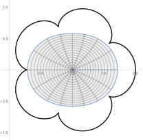
(a) $\mathcal{W}$

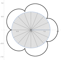
(b) $\mathcal{F}_{1}$

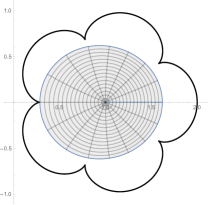
(c) $\mathcal{F}_{2}$

Figure 2. $\mathcal{S}^{*}_{n\mathcal{L}}-$radius for class $\mathcal{W}$, $\mathcal{F}_{1}$ and $\mathcal{F}_{2}$

Theorem 4.3.

For function in class $\mathcal{S}\mathcal{L}^{*}(\alpha),\,\mathcal{S}^{*}_{\alpha,e}$ and $\mathcal{S}^{*}_{EL}$, the following holds:

• $\mathcal{R}_{\mathcal{S}^{*}_{n\mathcal{L}}}\left(\mathcal{S}\mathcal{L}^{*}(\alpha)\right)=\displaystyle\frac{(n-1)\left(2\alpha(n+1)-n-3\right)}{(n+1)^{2}(\alpha-1)^{2}}.$
  

• $\mathcal{R}_{\mathcal{S}^{*}_{n\mathcal{L}}}\left(\mathcal{S}^{*}(\sqrt{1+cz})\right)=\displaystyle\frac{n^{2}+2n-3}{c(n+1)^{2}},$ for $1-\displaystyle\frac{4}{(n+1)^{2}}<c\leq 1.$
  

• $\mathcal{R}_{\mathcal{S}^{*}_{n\mathcal{L}}}\left(\mathcal{S}^{*}_{\alpha,e}\right)=\left|\log\left(\displaystyle\frac{1+\gamma^{n}+n+\gamma n+\alpha+n\alpha}{(n+1)(1-\alpha)}\right)\right|.$
  

• $\mathcal{R}_{\mathcal{S}^{*}_{n\mathcal{L}}}(\mathcal{S}^{*}_{EL})=\gamma^{n}+n\gamma+(n+1)\alpha-\phi(\delta)(1+n)(1-\alpha),$ where $\phi(z)$ gives the principal solution for $w$ in $z=we^{w}$ and $\delta=\alpha\exp((\gamma^{n}+n\gamma+\alpha(1+n))/(n+1)(1-\alpha))/(1-\alpha),$

for $\gamma=e^{i\pi/(n-1)}$ and $0\leq\alpha<1.$ All bounds are sharp.

Proof.

(a) Let $f\in\mathcal{S}\mathcal{L}^{*}(\alpha).$ Then $zf^{\prime}(z)/f(z)\prec\alpha+(1-\alpha)\sqrt{1+z}.$ The image of disk $|z|<r$ under the function $zf^{\prime}(z)/f(z)$ lies inside the domain $\varphi_{n\mathcal{L}}(\mathbb{D})$ if

$$\left|\frac{zf^{\prime}(z)}{f(z)}-1\right| \leq\left|\alpha+(1-\alpha)\sqrt{1+z}-1\right|$$

$$\leq(1-\alpha)\left(1-\sqrt{1-r}\right)$$

$$\leq 1-\frac{2}{n+1}.$$

This holds for $r\leq(n-1)\left(2\alpha(n+1)-n-3\right)/((n+1)^{2}.(\alpha-1)^{2})$. The result is sharp for the function $f_{n\mathcal{L}}(z)$ given by (1.3). Further,

$$\frac{zf_{n\mathcal{L}}^{\prime}(z)}{f_{n\mathcal{L}}(z)}=\frac{2}{n+1}=\varphi_{n\mathcal{L}}(-1),$$

for $z=(n-1)\left(2\alpha(n+1)-n-3\right)/((n+1)^{2}.(\alpha-1)^{2})$. For $\alpha=0,$ the sharpness is shown in Figure 3(a).

(b) For $0<c\leq 1-4/(n+1)^{2},$ the $\mathcal{S}^{*}_{n\mathcal{L}}-$radius for the class $\mathcal{S}^{*}(\sqrt{1+cz})$ is 1 by Theorem 3.1(d). Let us now assume that $1-4/(n+1)^{2}<c\leq 1.$ Since $f\in\mathcal{S}^{*}(\sqrt{1+cz}),$ we have

$$\left|\frac{zf^{\prime}(z)}{f(z)}-1\right|\leq 1-\sqrt{1-cr}.$$

By using Lemma 1.1, we get $1-\sqrt{1-cr}\leq 2/(n+1)$ and this simplifies to $r\leq(n^{2}+2n-3)/(c(n+1)^{2}).$

(c) For $f\in\mathcal{S}^{*}_{\alpha,e}$, we compute the radius by considering the geometries of the domains. The image of disk $|z|<r$ under the function $zf^{\prime}(z)/f(z)$ lies inside the domain $\varphi_{n\mathcal{L}}(\mathbb{D})$ if $r\leq r_{1},$ where $r_{1}$ is the absolute value of the solution of the equation $\alpha+(1-\alpha)e^{r}=\varphi_{n\mathcal{L}}(e^{i\pi/(n-1)}).$ A direct computation gives

$$r_{1}=\left|\log\left(\displaystyle\frac{1+\gamma^{n}+n+\gamma n+\alpha+n\alpha}{(n+1)(1-\alpha)}\right)\right|.$$

Clearly, the result is sharp and can be seen from Figure 3(b) for the particular case $\alpha=0$.

(d) Similarly, for this class, the $\mathcal{S}^{*}_{n\mathcal{L}}-$radius is obtained by solving the equation $\alpha e^{r}+(1-\alpha)(1+r)=\varphi_{n\mathcal{L}}(e^{i\pi/(n-1)})$ for $r.$ This gives that the desired result holds for $r\leq\mathcal{R}_{\mathcal{S}^{*}_{n\mathcal{L}}}(\mathcal{S}^{*}_{EL})$. For $a\alpha=1/2,$ the sharpness is shown in Figure 3(c). ∎

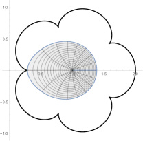
(a) $\mathcal{S}\mathcal{L}^{*}(0)$

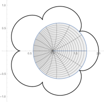
(b) $\mathcal{S}^{*}_{0,e}$

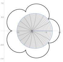
(c) $\mathcal{S}^{*}_{EL}(\alpha=1/2)$

Figure 3. $\mathcal{S}^{*}_{n\mathcal{L}}-$radius of classes $\mathcal{S}\mathcal{L}^{*}(0)$, $\mathcal{S}^{*}_{0,e}$ and $\mathcal{S}^{*}_{EL}(\alpha=1/2)$

Theorem 4.4.

The sharp $\mathcal{S}^{*}_{n\mathcal{L}}-$radius for various Ma-Minda type subclasses of starlike functions is given by

• $\mathcal{R}_{\mathcal{S}^{*}_{n\mathcal{L}}}\left(\mathcal{S}^{*}_{C}\right)=\left|\displaystyle\frac{\sqrt{16(n+1)^{2}+8(n+1)(3\gamma^{n}+3n\gamma)}}{4(n+1)}-1\right|$

• $\mathcal{R}_{\mathcal{S}^{*}_{n\mathcal{L}}}(\mathcal{S}^{*}_{\leftmoon})=\displaystyle\frac{1}{2}\left|\frac{2\gamma^{n-1}(n+1)+\gamma^{2n-1}+2\gamma^{n}+}{(1+n)(1+\gamma^{n}+n+n\gamma)}\right|$

• $\mathcal{R}_{\mathcal{S}^{*}_{n\mathcal{L}}}(\mathcal{S}^{*}_{R})=|R_{1}|/(2(n+1))$, where

  (4.2) $$R_{1}=(1+\sqrt{2})(\gamma^{n}+1+n+\gamma)+\\ \sqrt{(n+1)\left(3+2\sqrt{2}\right)\left(\gamma^{n}+n\gamma\right)+\left(1+\sqrt{2}\right)^{2}(1+n+n\gamma+\gamma^{n})^{2}}.$$

• $\mathcal{R}_{\mathcal{S}^{*}_{n\mathcal{L}}}(\mathcal{S}^{*}_{RL})=\displaystyle\frac{(n-1)(1-\sqrt{2}+3n+\sqrt{2}n)}{11-7\sqrt{2}+6n-6\sqrt{2}n+3n^{2}+\sqrt{2}n^{2}}$

• $\mathcal{R}_{\mathcal{S}^{*}_{n\mathcal{L}}}(\mathcal{S}^{*}_{lim})=\left|\sqrt{\displaystyle\frac{2(1+\gamma^{n}+n(1+\gamma))}{n+1}}-\sqrt{2}\right|$

• $\mathcal{R}_{\mathcal{S}^{*}_{n\mathcal{L}}}(\mathcal{S}^{*}(1+ze^{z}))=\left|\phi\left(\displaystyle\frac{\gamma^{n}+n\gamma}{1+n}\right)\right|,$ where $\phi(z)$ is given as in Theorem 5.5(c),
  

• $\mathcal{R}_{\mathcal{S}^{*}_{n\mathcal{L}}}(\mathcal{S}^{*}_{car})=\left|-1+\sqrt{\displaystyle\frac{1+2\gamma^{n}+n+2\gamma n}{n+1}}\right|.$

where $\gamma=e^{i\pi/(n-1)}.$

Proof.

(a) Let $f\in\mathcal{S}^{*}_{C}$. Then $zf^{\prime}(z)/f(z)\prec 1+4z/3+2z^{2}/3.$ By geometric interpretation, the cardiod $(9u^{2}+9v^{2}-18u+5)^{2}-16(9u^{2}+9v^{2}-6u+1)=0$ lies in the domain $\varphi_{n\mathcal{L}}(\mathbb{D})$ for $r\leq r_{3},$ where $r_{3}$ is the absolute solution of the equation

$$\frac{4r}{3}+\frac{2r^{2}}{3}=\frac{ne^{i\pi/(n-1)}}{n+1}+\frac{e^{in\pi/(n-1)}}{n+1},$$

given by

$$r_{3}=\left|-1+\frac{\sqrt{4(n+1)^{2}+6(n+1)(\gamma^{n}+n\gamma)}}{n+1}\right|,$$

for $\gamma=e^{i\pi/(n-1)}.$ Sharpness can be seen from Figure 4(a).

(b) Proceeding in a similar way, the necessary condition for the lune $|w^{2}-1|<2|w|,\,w\in\mathbb{C},$ to lie inside the domain $\varphi_{n\mathcal{L}}(\mathbb{D})$ is obtained by solving $r+\sqrt{1+r^{2}}=\varphi_{n\mathcal{L}}(e^{i\pi/(n-1)})$ for $r$. A direct simplification yields the $\mathcal{S}^{*}_{n\mathcal{L}}-$radius for this class is $r_{4}$ which is exactly $\mathcal{R}_{\mathcal{S}^{*}_{n\mathcal{L}}}(\mathcal{S}^{*}_{\leftmoon})$ (See Figure 4(b)).

(c) Similarly, for this class, the $\mathcal{S}^{*}_{n\mathcal{L}}-$ radius is computed by solving equation

$$\frac{(\sqrt{2}+1)^{2}+r^{2}}{(\sqrt{2}+1)(\sqrt{2}+1-r)}=1+\frac{ne^{i\pi/(n-1)}}{n+1}+\frac{e^{in\pi/(n-1)}}{n+1},$$

for $r$. This gives $r\leq|R_{1}|/(2(n+1)),$ where $R_{1}$ is given by (4.2). The sharpness for this class is depicted in Figure 4(c).

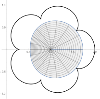
(a) $\mathcal{S}^{*}_{car}$

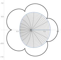
(b) $\mathcal{S}^{*}_{\leftmoon}$

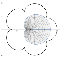
(c) $\mathcal{S}^{*}_{R}$

Figure 4. $\mathcal{S}^{*}_{n\mathcal{L}}-$radius for $\mathcal{S}^{*}_{car}$, $\mathcal{S}^{*}_{\leftmoon}$ and $\mathcal{S}^{*}_{R}$

(d) Let $f\in\mathcal{S}^{*}_{RL}.$ Then the image of the disk $|z|<r$ under the function $zf^{\prime}(z)/f(z)$ lies in the domain $\varphi_{n\mathcal{L}}(\mathbb{D})$ for $r\leq r_{4},$ where $r_{4}$ is the solution of the equation

$$\sqrt{2}-(\sqrt{2}-1)\sqrt{\frac{1-r}{1+2(\sqrt{2}-1)r}}=\frac{2}{n+1},$$

by geometries of the domains. The result is sharp for the function $f_{4}$ defined such that

$$\frac{zf_{4}^{\prime}(z)}{f_{4}(z)}=\sqrt{2}-(\sqrt{2}-1)\sqrt{\frac{1-z}{1+2(\sqrt{2}-1)z}}.$$

It is clear that

$$\left.\frac{zf_{4}^{\prime}(z)}{f_{4}(z)}\right|_{z=r_{4}}=\frac{2}{n+1}=\varphi_{n\mathcal{L}}(-1),$$

as illustrated in Figure 5(a).

(e) To compute this radius, we solve the following equation for r

$$\sqrt{2}r+\frac{r^{2}}{2}=\frac{ne^{i\pi/(n-1)}}{n+1}+\frac{e^{in\pi/(n-1)}}{n+1}.$$

Thus, $\mathcal{S}^{*}_{n\mathcal{L}}-$radius for the class $\mathcal{S}^{*}_{lim}$ is given by $\mathcal{R}_{\mathcal{S}^{*}_{n\mathcal{L}}}(\mathcal{S}^{*}_{lim})$ and sharpness is shown in Figure 5(b).

(f) The $\mathcal{S}^{*}_{n\mathcal{L}}-$radius for the class $\mathcal{S}^{*}(1+ze^{z})$ by solving the equation $1+re^{r}=\varphi_{n\mathcal{L}}(e^{i\pi/(n-1)})$ for $r$. This gives the desired result holds for $r\leq\phi((\gamma^{n}+n\gamma)/(n+1))$ where the function $\phi$ is defined in Theorem 5.5(c). (See Figure 5(c)).

(g) Lastly, to compute the $\mathcal{S}^{*}_{n\mathcal{L}}-$radius for this class we will consider the cusp at the angle $\pi/(n-1)$ and obtain the equation

$$(n+1)(2r+r^{2})=2(ne^{i\pi/(n-1)}+e^{in\pi/(n-1)}).$$

On solving above equation, we get the desired result holds for $r\leq\mathcal{R}_{\mathcal{S}^{*}_{n\mathcal{L}}}(\mathcal{S}^{*}_{car}),$ given in the statement of the theorem. Sharpness is depicted in Figure 5(d). ∎

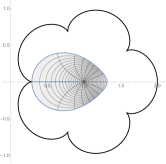
(a) $\mathcal{S}^{*}_{RL}$

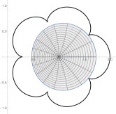
(b) $\mathcal{S}^{*}_{lim}$

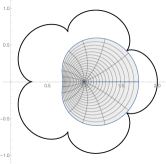
(c) $\mathcal{S}^{*}(1+ze^{z})$

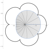
(d) $\mathcal{S}^{*}_{car}$

Figure 5. Sharpness of $\mathcal{S}^{*}_{n\mathcal{L}}$ radii for various classes

Theorem 4.5.

Let $n=2k,\,k\in\mathbb{N}.$ Then

• The $\mathcal{S}^{*}_{n\mathcal{L}}-$radius for the class $\mathcal{S}^{*}_{sin}$ is given by $\mathcal{R}_{\mathcal{S}^{*}_{n\mathcal{L}}}(\mathcal{S}^{*}_{sin})=|R_{2}|,$ where

  (4.3) $$R_{2}=\begin{cases}\sin^{-1}\left(\displaystyle\frac{\gamma^{k}(\gamma^{(n-1)}+n)}{n+1}\right),&k\text{ is odd},\\ \\ \sin^{-1}\left(\displaystyle\frac{\gamma^{(k-1)}(\gamma^{(n-1)}+n)}{n+1}\right),&k\text{ is even}.\end{cases}$$

• The $\mathcal{S}^{*}_{n\mathcal{L}}-$radius for the class $\mathcal{S}^{*}_{ne}$ is given by $\mathcal{R}_{\mathcal{S}^{*}_{n\mathcal{L}}}(\mathcal{S}^{*}_{ne})=|R_{3}|,$ where

  (4.4) $$R_{3}=\begin{cases}\displaystyle\frac{\left(1+i\sqrt{3}\right)(n+1)}{2^{2/3}\delta_{1}}+\displaystyle\frac{\left(1-i\sqrt{3}\right)\delta_{1}}{2^{2/3}(n+1)},&k\text{ is odd},\\ \\ \displaystyle\frac{\left(1-i\sqrt{3}\right)(n+1)}{2^{2/3}\delta_{2}}+\displaystyle\frac{\left(1+i\sqrt{3}\right)\delta_{2}}{2^{2/3}(n+1)},&k\text{ is even},\end{cases}$$

  where

  (4.5) $$\delta_{1} =\left(3(n+1)^{2}(\gamma^{kn}+\gamma^{k}n)+(n+1)^{2}\sqrt{9\gamma^{k}\left(\gamma^{2}n+2\gamma^{n+1}+\gamma^{2}n^{2})-4(n+1)^{2}\right)}\right)^{2/3}$$

  (4.6) $$\delta_{2} =\left(3(n+1)^{2}\left(\gamma^{n(k-1)}+n\gamma^{k-1}\right)+(n+1)^{2}\sqrt{9\gamma^{k-1}\left(\gamma^{2n}+2\gamma^{n+1}n+\gamma^{2}n^{2}\right)-4(n+1)^{2}}\right)^{2/3}$$

Here $\gamma=e^{i\pi/(n-1)}.$

Proof.

(a) Let $f\in\mathcal{S}^{*}_{sin}$ and $n=2k,\,k\in\mathbb{N}.$ Let $k$ be odd. In this case, the cusp considered is at the angle $k\pi/(n-1).$ Thus the image of $zf^{\prime}(z)/f(z)$ under $\mathbb{D}_{r}$ lies in the domain $\varphi_{n\mathcal{L}}(\mathbb{D})$ for $r\leq|R_{2}|,$ where

$$R_{2}=\sin^{-1}\left(\displaystyle\frac{\gamma^{k}(\gamma^{(n-1)}+n)}{n+1}\right),$$

is the solution of the equation $\sin r(n+1)=ne^{ik\pi/(n-1)}+e^{ink\pi/(n-1)}.$ Proceeding in a similar way, we will consider the cusp at the angle $(k-1)\pi/(n-1)$ for the case when $k$ is even. The $\mathcal{S}^{*}_{n\mathcal{L}}-$radius is obtained by solving the equation $\sin r(n+1)=ne^{i(k-1)\pi/(n-1)}+e^{in(k-1)\pi/(n-1)}$ for $r$. This gives $r\leq|R_{2}|,$ where

$$\sin^{-1}\left(\displaystyle\frac{\gamma^{(k-1)}(\gamma^{(n-1)}+n)}{n+1}\right).$$

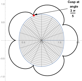
(a) $n=6$

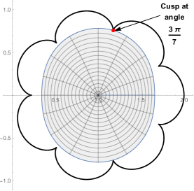
(b) $n=8$

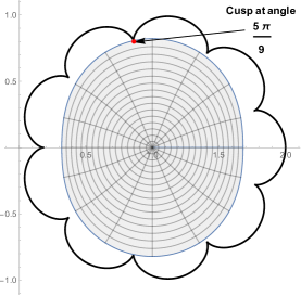
(c) $n=10$

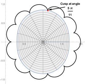
(d) $n=12$

Figure 6. Image of $\varphi_{sin}(z)$ lying in various polyleaf domain

For some choices $n$, sharpness for the above result is depicted in the Figure 6.

(b) Let $n=2k,\,k\in\mathbb{N}.$ Let us first consider the case when $k$ is odd. In this case, the desired radius is computed by considering the cusp at the angle $k\pi/(n-1).$ Thus, the image of the disk $|z|<r$ under the function $zf^{\prime}(z)/f(z)$ lies in the domain $\varphi_{n\mathcal{L}}(\mathbb{D})$ for $r\leq|R_{3}|,$ where $R_{3}$ is the solution of the equation $(n+1)(3r-r^{3})=3(ne^{ik\pi/(n-1)}+e^{ink\pi/(n-1)})$ given by

$$R_{3}=\frac{\left(1+i\sqrt{3}\right)(n+1)}{2^{2/3}\delta_{1}}+\displaystyle\frac{\left(1-i\sqrt{3}\right)\delta_{1}}{2^{2/3}(n+1)},$$

where $\delta_{1}$ is given by (4.5). Let us now assume that $k$ is even. We will consider the cusp at the angle $(k-1)\pi/(n-1).$ In this case, the $\mathcal{S}^{*}_{n\mathcal{L}}-$radius for the class $\mathcal{S}^{*}_{ne}$ is computed by solving the equation $(n+1)(3r-r^{3})=3(ne^{i(k-1)\pi/(n-1)}+e^{in(k-1)\pi/(n-1)})$ for $r$. This gives $r\leq|R_{3}|,$ where

$$R_{3}=\frac{\left(1-i\sqrt{3}\right)(n+1)}{2^{2/3}\delta_{2}}+\displaystyle\frac{\left(1+i\sqrt{3}\right)\delta_{2}}{2^{2/3}(n+1)},$$

where $\delta_{2}$ is given by (4.6). The sharpness is illustrated for some choices of $n$ in the Figure 7.

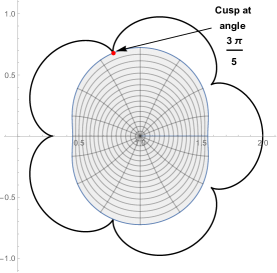
(a) $n=6$

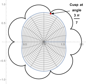
(b) $n=8$

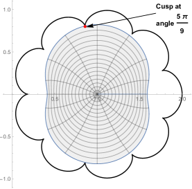
(c) $n=10$

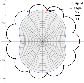
(d) $n=12$

Figure 7. Nephroid domain lying in various polyleaf domain

∎

The next theorem gives the $\mathcal{S}^{*}_{n\mathcal{L}}-$radius for some special Janowski classes. As proves earlier, this result is also obtained by considering the cusp at the angle $\pi/(n-1)$ and hence omitted here.

Theorem 4.6.

The $\mathcal{S}^{*}_{n\mathcal{L}}-$radius for some special Janowski classes is given by

• $\mathcal{R}_{\mathcal{S}^{*}_{n\mathcal{L}}}(\mathcal{S}^{*}(\alpha))=\left|\displaystyle\frac{\gamma^{n}+n\gamma}{2(1-\alpha)+\gamma^{n}+2n(1-\alpha)+n\gamma}\right|$

• $\mathcal{R}_{\mathcal{S}^{*}_{n\mathcal{L}}}(\mathcal{S}^{*}[\alpha,-\alpha])=\left|\displaystyle\frac{\gamma^{n}+n\gamma}{\alpha(2+\gamma^{n}+2n+n\gamma)}\right|,$ where $0<\alpha\leq 1.$

• $\mathcal{R}_{\mathcal{S}^{*}_{n\mathcal{L}}}(\mathcal{S}^{*}[1-\alpha,0])=\left|\displaystyle\frac{\gamma^{n}+n\gamma}{(n+1)(1-\alpha)}\right|$

• $\mathcal{R}_{\mathcal{S}^{*}_{n\mathcal{L}}}(\mathcal{S}^{*}[1,-(M-1)/M])=\left|\displaystyle\frac{M(\gamma^{n}+n\gamma)}{-1+2M-\gamma^{n}+M\gamma^{n}-n+2Mn-\gamma n+Mn\gamma}\right|,$ for $M>1/2.$

Remark 4.7.

For $\alpha=0,$ the above result gives the $\mathcal{S}^{*}_{n\mathcal{L}}-$radius for the class $\mathcal{S}^{*}$ of starlike function and it is given by $|(\gamma^{n}+n\gamma)/(2+\gamma^{n}+2n+n\gamma)|,$ where $\gamma=e^{i\pi/(n-1)}.$ By using Mark Strohhacker’s theorem, it is known that $\mathcal{K}\subset\mathcal{S}^{*}(1/2).$ Thus, the $\mathcal{S}^{*}_{n\mathcal{L}}-$radius for the class $\mathcal{K}$ is atleast $|(\gamma^{n}+n\gamma)/(1+\gamma^{n}+n+n\gamma)|.$

Remark 4.8.

The $\mathcal{S}^{*}_{n\mathcal{L}}-$radius for the classes $\mathcal{S}^{*}_{SG}$, $\mathcal{S}^{*}(\cos z)$ and $\mathcal{S}^{*}(\cosh z)$ is $1$ as these domains lie inside the domain $\varphi_{n\mathcal{L}}(\mathbb{D})$ (as depicted by Figure 8).

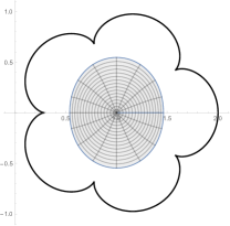
(a) $\mathcal{S}^{*}_{SG}$

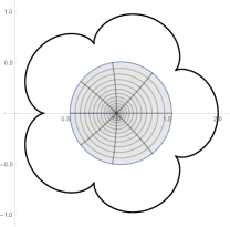
(b) $\mathcal{S}^{*}(\cos z)$

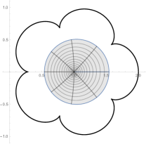
(c) $\mathcal{S}^{*}(\cosh z)$

Figure 8. Domains lying inside $\varphi_{n\mathcal{L}}(\mathbb{D})$

Remark 4.9.

As mentioned earlier, the class $\mathcal{S}^{*}_{n\mathcal{L}}$ becomes the class $\mathcal{S}^{*}[1,0]$ for which the image domain is a disk with center $1$ and radius $1$ in the limiting case. Thus, $\mathcal{S}^{*}[1,0]-$radius for various classes can be obtained by taking the limit as $n\rightarrow\infty$ in the above proved results. The following table summarizes the $\mathcal{S}^{*}[1,0]-$radii.

S.No. Class $n\rightarrow\infty$ $\displaystyle(a)$ $\displaystyle\mathcal{W}$ $\sqrt{2}-1$ $\displaystyle(b)$ $\displaystyle\mathcal{F}_{1}$ $\sqrt{5}-2$ $\displaystyle(c)$ $\displaystyle\mathcal{F}_{2}$ $(\sqrt{17}-3)/4$ $\displaystyle(d)$ $\displaystyle\mathcal{S}^{*}_{RL}$ $1$ $\displaystyle(e)$ $\displaystyle\mathcal{S}^{*}_{C}$ $\sqrt{5/2}-1$ $\displaystyle(f)$ $\displaystyle\mathcal{S}^{*}_{R}$ $-1-\sqrt{2}+\sqrt{6+4\sqrt{2}}$ $\displaystyle(g)$ $\displaystyle\mathcal{S}^{*}_{\leftmoon}$ $3/4$ $\displaystyle(h)$ $\displaystyle\mathcal{S}^{*}_{lim}$ $2-\sqrt{2}$ $\displaystyle(i)$ $\displaystyle\mathcal{S}^{*}(1+ze^{z})$ $0.567143$

S.No. Class $n\rightarrow\infty$ $\displaystyle(a)$ $\displaystyle\mathcal{M}(\beta)$ $1/(2\beta-1)$ $\displaystyle(b)$ $\displaystyle\mathcal{B}\mathcal{S}(\alpha)$ $(1+\sqrt{1+4\alpha})/2\alpha$ $\displaystyle(c)$ $\displaystyle\mathcal{S}\mathcal{L}^{*}(\alpha)$ $(2\alpha-1)/(\alpha-1)^{2}$ $\displaystyle(d)$ $\displaystyle\mathcal{S}^{*}_{\alpha,e}$ $\log((\alpha-2)/(\alpha-1))$ $\displaystyle(e)$ $\displaystyle\mathcal{S}^{*}(\alpha)$ $1/(3-2\alpha)$ $\displaystyle(f)$ $\displaystyle\mathcal{S}^{*}[1-\alpha,0]$ $1/(\alpha-1)$ $\displaystyle(g)$ $\displaystyle\mathcal{S}^{*}[\alpha,-\alpha]$ $1/(3\alpha)$ $\displaystyle(h)$ $\displaystyle\mathcal{S}^{*}_{M}$ $M/(3M-2)$

Table 1. Radii for the Limiting case

5. Radius Constants for class $\mathcal{S}^{*}_{n\mathcal{L}}$

Theorem 5.1.

The sharp radii constants for the class $\mathcal{S}^{*}_{n\mathcal{L}}$ as follows

• The $\mathcal{S}\mathcal{L}^{*}(\alpha)-$radius is the smallest positive real root of the equation $r^{n}+rn-(\sqrt{2}-1)(1-\alpha)(n+1)=0,$ for $0\leq\alpha<1$.

• The $\mathcal{S}^{*}_{RL}-$radius is the smallest positive real root of the equation $r^{n}+rn-(n+1)\left(\sqrt{\gamma}-\gamma\right)^{1/2}=0$, where $\gamma=2\sqrt{2}-2.$

• The $\mathcal{S}^{*}_{R}-$radius is the smallest positive real root of the equation $r^{n}-rn-(n+1)(2\sqrt{2}+3)=0$.

• The $\mathcal{S}^{*}_{sin}-$radius is the smallest positive real root of the equation $r^{n}+rn-(n+1)\sin 1=0$.

• The $\mathcal{S}^{*}_{SG}-$radius is the smallest positive real root of the equation $r^{n}+rn-(n+1)(e-1)/(e+1)=0.$

• The $\mathcal{S}^{*}_{ne}-$radius is the smallest positive real root of the equation $r^{n}+rn-2(n+1)/3=0.$

• The $\mathcal{S}^{*}(1+ze^{z})-$radius is the smallest positive real root of the equation $r^{n}-rn+(n+1)/e=0.$

• The $\mathcal{S}^{*}(1+\sinh^{-1}(z))-$radius is the smallest positive real root of the equation $r^{n}+rn-(n+1)\sinh^{-1}(1)=0.$

• The $\mathcal{M}(\beta)-$radius is the smallest positive real root of the equation $r^{n}+rn-(n+1)(\beta-1)=0,$ for $1<\beta\leq 2$ and the radius is $1,$ for $\beta\geq 2.$

• The $\mathcal{S}^{*}[1-\alpha,0]-$radius is the smallest positive real root of the equation $r^{n}+rn-(n+1)(1-\alpha)=0.$

Proof.

Let $f\in\mathcal{S}^{*}_{n\mathcal{L}}.$ Then $zf^{\prime}(z)/f(z)\prec\varphi_{n\mathcal{L}},$ where $\varphi_{n\mathcal{L}}$ is given by (1.2). For $|z|=re^{it},$

(5.1) $$\left|\frac{zf^{\prime}(z)}{f(z)}-1\right|\leq\frac{nr}{n+1}+\frac{r^{n}}{n+1}.$$

(a) By using [10, Lemma 2.3, pp 6], it can be obtained that the disk (5.1) lies inside the lemniscate of Bernoulli $|((w-\alpha)/(1-\alpha))^{2}-1|=1$ if

$$\frac{nr}{n+1}+\frac{r^{n}}{n+1}\leq(\sqrt{2}-1)(1-\alpha).$$

This gives $r\leq s_{1},$ where $s_{1}$ is the smallest positive real root of the equation $r^{n}+rn-(\sqrt{2}-1)(1-\alpha)(n+1)=0,$ for $0\leq\alpha<1$. For sharpness, consider the function $f_{n\mathcal{L}}(z)$ given by (1.3). The value of $zf_{n\mathcal{L}}^{\prime}(z)/f_{n\mathcal{L}}(z)$ is $\sqrt{2},$ for $z=s_{1}.$

(b) The disk (5.1) lies in the left-hand side of reverse lemniscate of Bernoulli $|(w-\sqrt{2})^{2}-1|=1$ if

$$\frac{nr}{n+1}+\frac{r^{n}}{n+1}\leq\sqrt{\sqrt{2\sqrt{2}-2}-2\sqrt{2}+2},$$

by [18, Lemma 3.2, pp 10]. This simplifies to $r\leq s_{2},$ where $s_{2}$ is the smallest positive real root of the equation $r^{n}+rn-(n+1)\left(\sqrt{\gamma}-\gamma\right)^{1/2}=0$, where $\gamma=2\sqrt{2}-2.$ The result is sharp for the function $f_{n\mathcal{L}}$ given by (1.3).

(c) The subordination $\varphi_{n\mathcal{L}}(z)\prec\varphi_{R}(z)$ holds for $\mathbb{D}_{r}$ if

$$2(\sqrt{2}-1)\leq\varphi_{R}(-1)\leq\varphi_{n\mathcal{L}}(-r)=1-\frac{nr}{n+1}+\frac{r^{n}}{n+1},$$

for $n$ is even. This gives $r\leq s_{3},$ where $s_{3}$ is the smallest positive real root of the equation $r^{n}-rn-(n+1)(2\sqrt{2}+3)=0$.The bound is best possible for the function $f_{n\mathcal{L}}$ given by (1.3). For $z=s_{3},$ the quantity $zf_{n\mathcal{L}}^{\prime}(z)/f_{n\mathcal{L}}(z)=2(\sqrt{2}-1).$

(d) Similarly, the disk (5.1) lies in the image domain of $\varphi_{sin}(\mathbb{D})$ if

$$1+\frac{nr}{n+1}+\frac{r^{n}}{n+1}\leq\varphi_{n\mathcal{L}}(r)\leq\varphi_{sin}(1)=1+\sin 1.$$

This holds for $r\leq s_{4},$ where $s_{4}$ is the smallest positive real root of the equation $r^{n}+rn-(n+1)\sin 1=0$. The result is best possible for the function $f_{n\mathcal{L}}(z)$ given by (1.3) and $zf_{n\mathcal{L}}^{\prime}(z)/f_{n\mathcal{L}}(z)=1+\sin 1,$ for $z=s_{4}.$

(e) By [4, Lemma 2.2, pp 5], the disk (5.1) lies in the modified sigmoid $|\log(w/(2-w))|=1$ if

$$\frac{nr}{n+1}+\frac{r^{n}}{n+1}\leq\frac{e-1}{e+1}.$$

This simplifies to $r\leq s_{5},$ where $s_{5}$ is the smallest positive real root of the equation $r^{n}+rn-(n+1)(e-1)/(e+1)=0.$ The bound cannot be improved further as for $z=s_{5},$ $zf_{n\mathcal{L}}^{\prime}(z)/f_{n\mathcal{L}}(z)$ assumes value $2e/(e+1),$ where $f_{n\mathcal{L}}(z)$ is given by (1.3).

(f) [31, Lemma 2.2, pp 8] gives the following condition for the disk (5.1) to lie inside the nephroid

$$\frac{nr}{n+1}+\frac{r^{n}}{n+1}\leq\frac{2}{3}.$$

This gives $r\leq s_{6},$ where $s_{6}$ is the smallest positive real root of the equation $r^{n}+rn-2(n+1)/3=0.$ For sharpness, consider the function $f_{n\mathcal{L}}(z)$ given by (1.3). For $z=s_{6},$ the value of $zf_{n\mathcal{L}}^{\prime}(z)/f_{n\mathcal{L}}(z)$ is $5/3.$

(g) For $|z|<r,$ a necessary condition for the subordination $\varphi_{n\mathcal{L}}(z)\prec 1+ze^{z}$ to hold is

$$1-\frac{1}{e}\leq\varphi_{n\mathcal{L}}(-r)=1-\frac{nr}{n+1}+\frac{r^{n}}{n+1}.$$

This simplifies to $r\leq s_{7},$ where $s_{7}$ is the smallest positive real root of the equation $r^{n}-rn+(n+1)/e=0.$ The result is sharp for the function $f_{n\mathcal{L}}(z)$ given by (1.3) and $zf_{n\mathcal{L}}^{\prime}(z)/f_{n\mathcal{L}}(z)=1-1/e,$ for $z=-s_{7}.$

(h) By using [27, Lemma 2.1, pp 4], we get the disk (5.1) lie inside the image domain of the function $1+\sinh^{-1}(z)$ if

$$\frac{r^{n}}{n+1}+\frac{nr}{n+1}\leq\sinh^{-1}(1),$$

which simplifies to $r\leq s_{8},$ where $s_{8}$ is the smallest positive real root of the equation $r^{n}+rn-(n+1)\sinh^{-1}(1)=0.$ The bounds are sharp for the function $f_{n\mathcal{L}}(z)$ given by (1.3). For $z=s_{8},$ $zf_{n\mathcal{L}}^{\prime}(z)/f_{n\mathcal{L}}(z)=1+\sinh^{-1}(1).$

(i) As seen earlier, $\mathcal{S}^{*}_{n\mathcal{L}}\subset\mathcal{M}(\beta)$ for $\beta>2.$ Let us now assume that $1<\beta\leq 2.$ For $|z|=r<1,$

$$\operatorname{Re}\left(\frac{zf^{\prime}(z)}{f(z)}\right)<1+\frac{nr}{n+1}+\frac{r^{n}}{n+1}<\beta,$$

provided $r<s_{9},$ where $s_{9}$ is the smallest positive real root of the equation $r^{n}+rn-(n+1)(\beta-1)=0$. For the function $f_{n\mathcal{L}}$, the quantity $zf_{n\mathcal{L}}^{\prime}(z)/f_{n\mathcal{L}}(z)=\beta$ at $z=s_{9}.$

(j) The disk (5.1) lies in the domain $|w-1|<1-\alpha$ if

$$\frac{r^{n}}{n+1}+\frac{nr}{n+1}\leq 1-\alpha,$$

which gives $r\leq s_{10},$ where $s_{10}$ is the smallest positive real root of the equation $r^{n}+rn-(n+1)(1-\alpha)=0.$ The result is sharp for the function $f_{n\mathcal{L}}(z)$ given by (1.3) and for $z=s_{10},$ $zf_{n\mathcal{L}}^{\prime}(z)/f_{n\mathcal{L}}(z)=2-\alpha.$

For some choices of $n$, the radii are computed is tabulated in Table 2 and the sharpness for these results is illustrated by Figure 9 for $n=8.$ ∎

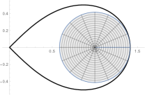
(a) $\mathcal{S}^{*}_{L}$

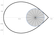
(b) $\mathcal{S}^{*}_{RL}$

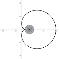
(c) $\mathcal{S}^{*}_{R}$

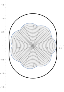
(d) $\mathcal{S}^{*}_{sin}$

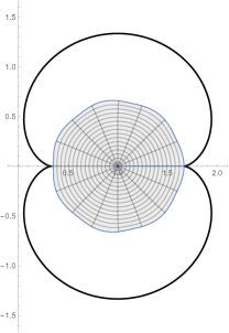
(e) $\mathcal{S}^{*}_{ne}$

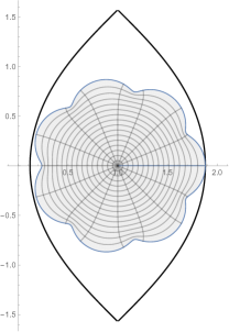
(f) $\mathcal{S}^{*}(1+\sinh^{-1}(z))$

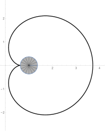
(g) $\mathcal{S}^{*}(1+ze^{z})$

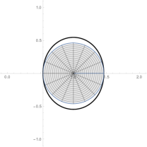
(h) $\mathcal{S}^{*}_{SG}$

Figure 9. Sharpness of various radii for class $\mathcal{S}^{*}_{n\mathcal{L}}$

S.No.	Class	n=4	n=6	n=8
$\displaystyle(a)$	$\displaystyle\mathcal{S}\mathcal{L}^{*}$	$0.501903$	$0.48118$	$0.465714$
$\displaystyle(b)$	$\displaystyle\mathcal{S}^{*}_{RL}$	$0.353501$	$0.333349$	$0.32165$
$\displaystyle(c)$	$\displaystyle\mathcal{S}^{*}_{R}$	$0.213942$	$0.200158$	$0.193019$
$\displaystyle(d)$	$\displaystyle\mathcal{S}^{*}_{sin}$	$0.892917$	$0.895669$	$0.895131$
$\displaystyle(e)$	$\displaystyle\mathcal{S}^{*}_{SG}$	$0.554083$	$0.535219$	$0.519222$
$\displaystyle(f)$	$\displaystyle\mathcal{S}^{*}_{ne}$	$0.752971$	$0.748475$	$0.738894$
$\displaystyle(g)$	$\displaystyle\mathcal{S}^{*}(1+ze^{z})$	$0.472288$	$0.43025$	$0.413972$
$\displaystyle(h)$	$\displaystyle\mathcal{S}^{*}(1+\sinh^{-1}(z))$	$0.921471$	$0.924325$	$0.924715$

Table 2. Radii constants for choices of $n$

References

- [1] R. M. Ali, N. K. Jain and V. Ravichandran, On the radius constants for classes of analytic functions, Bull. Malays. Math. Sci. Soc. (2) 36 (2013), no. 1, 23–38.
- [2] N. E. Cho, V. Kumar, S. S. Kumar and V. Ravichandran, Radius problems for starlike functions associated with the sine function, Bull. Iranian Math. Soc. 45 (2019), no. 1, 213–232.
- [3] S. Gandhi, Radius estimates for three leaf function and convex combination of starlike functions, In: Deo N., Gupta V., Acu A., Agrawal P. (eds) Mathematical Analysis I: Approximation Theory. ICRAPAM 2018. Springer Proceedings in Mathematics and Statistics, vol 306. Springer, Singapore, 2020.
- [4] P. Goel and S. S. Kumar, Certain Class of Starlike Functions Associated with Modified Sigmoid Function, Bull. Malays. Math. Sci. Soc. 43 (2020), no. 1, 957–991.
- [5] P. Gupta, S. Nagpal and V. Ravichandran, Inclusion relations and radius problems for a subclass of starlike functions, arXiv:2012.13511.
- [6] H. Hagen, Curve and surface design, Geometric Design Publications, Society for Industrial and Applied Mathematics (SIAM), Philadelphia, PA, 1992.
- [7] S. Kanas and A. Wisniowska, Conic regions and -uniform convexity, J. Comput. Appl. Math. 105 (1999), no. 1-2, 327–336.
- [8] R. Kargar, A. Ebadian and J. Sokół, On Booth lemniscate and starlike functions, Anal. Math. Phys. 9 (2019), no. 1, 143–154.
- [9] F. R. Keogh and E. P. Merkes, A coefficient inequality for certain classes of analytic functions, Proc. Amer. Math. Soc. 20 (1969), 8–12.
- [10] K. Khatter, V. Ravichandran and S. Sivaprasad Kumar, Starlike functions associated with exponential function and the lemniscate of Bernoulli, Rev. R. Acad. Cienc. Exactas Fís. Nat. Ser. A Mat. RACSAM 113 (2019), no. 1, 233–253.
- [11] S. Kumar and V. Ravichandran, A subclass of starlike functions associated with a rational function, Southeast Asian Bull. Math. 40 (2016), no. 2, 199–212.
- [12] J. D. Lawrence, A catalog of special plane curves, Dover Publications, 1972.
- [13] W. C. Ma and D. Minda, A unified treatment of some special classes of univalent functions, in Proceedings of the Conference on Complex Analysis (Tianjin, 1992), 157–169, Conf. Proc. Lecture Notes Anal., I, Int. Press, Cambridge, MA.
- [14] T. H. MacGregor, Functions whose derivative has a positive real part, Trans. Amer. Math. Soc. 104 (1962), 532–537.
- [15] T. H. MacGregor, The radius of univalence of certain analytic functions, Proc. Amer. Math. Soc. 14 (1963), 514–520.
- [16] T. H. MacGregor, The radius of univalence of certain analytic functions. II, Proc Amer. Math. Soc. 14 (1963), 521–524.
- [17] J. S. Madachy, Madachy’s Mathematical Recreations, New York: Dover, pp. 219-225, 1979.
- [18] R. Mendiratta, S. Nagpal and V. Ravichandran, A subclass of starlike functions associated with left-half of the lemniscate of Bernoulli, Internat. J. Math. 25 (2014), no. 9, 1450090, 17 pp.
- [19] R. Mendiratta, S. Nagpal and V. Ravichandran, On a subclass of strongly starlike functions associated with exponential function, Bull. Malays. Math. Sci. Soc. 38 (2015), no. 1, 365–386.
- [20] S. S. Miller and P. T. Mocanu, Differential subordinations, Monographs and Textbooks in Pure and Applied Mathematics, 225, Marcel Dekker, Inc., New York, 2000.
- [21] D. V. Prokhorov and J. Szynal, Inverse coefficients for -convex functions, Ann. Univ. Mariae Curie-Skłodowska Sect. A 35 (1981), 125–143 (1984).
- [22] R. K. Raina and J. Sokół, Some properties related to a certain class of starlike functions, C. R. Math. Acad. Sci. Paris 353 (2015), no. 11, 973–978.
- [23] V. Ravichandran and S. Verma, Bound for the fifth coefficient of certain starlike functions, C. R. Math. Acad. Sci. Paris 353 (2015), no. 6, 505–510.
- [24] K. Sharma, N. K. Jain and V. Ravichandran, Starlike functions associated with a cardioid, Afr. Mat. 27 (2016), no. 5-6, 923–939.
- [25] P. Sharma, R. K. Raina and J. Sokół, Certain Ma–Minda type classes of analytic functions associated with the crescent-shaped region, Anal. Math. Phys. 9 (2019), no. 4, 1887–1903.
- [26] S. Sivaprasad Kumar, K. Gangania, A Cardioid Domain and Starlike Functions, arXiv:2008.06833, (2020), 28 pages.
- [27] S. Sivaprasad Kumar, Kush Arora, Starlike Functions associated with a Petal Shaped Domain, arXiv:2010.10072, (2020), 15 pages.
- [28] J. Sokół and J. Stankiewicz, Radius of convexity of some subclasses of strongly starlike functions, Zeszyty Nauk. Politech. Rzeszowskiej Mat. No. 19 (1996), 101–105.
- [29] J. Sokół, On some subclass of strongly starlike functions, Demonstratio Math. 31 (1998), no. 1, 81–86.
- [30] B. A. Uralegaddi, M. D. Ganigi and S. M. Sarangi, Univalent functions with positive coefficients, Tamkang J. Math. 25 (1994), no. 3, 225–230.
- [31] L. A. Wani and A. Swaminathan, Radius problems for functions associated with a nephroid domain, Rev. R. Acad. Cienc. Exactas Fís. Nat. Ser. A Mat. RACSAM 114 (2020), no. 4, 178.
- [32] Y. Yunus, S. A. Halim and A. B. Akbarally, Subclass of starlike functions associated with a limacon, in AIP Conference Proceedings 2018 Jun 28 (Vol. 1974, No. 1, p. 030023), AIP Publishing.