The Exact WKB and the Landau-Zener transition for asymmetry in cosmological particle production

Abstract

Cosmological particle production by a time-dependent scalar field is common in cosmology. We focus on the mechanism of asymmetry production when interaction explicitly violates symmetry and its motion is rapid enough to create particles by itself. Combining the exact WKB analysis and the Landau-Zener transition, we point out that perturbation before the non-perturbative analysis may drastically change the structure of the Stokes lines of the theory. The Exact WKB can play an important role in avoiding such discrepancies.

I Introduction

In 1991, Cohen, Kaplan and Nelson proposed a mechanism of “Spontaneous Baryogenesis” for producing baryons at the electroweak phase transition in the adiabatic limit of thick slowly moving bubble wallsCohen:1991iu . Their original ideaCohen:1987vi ; Cohen:1988kt uses an effective chemical potential for biasing the baryon number, and the effective chemical potential was brought in by considering a time-dependent parameter. The mechanism avoids the “out of thermal equilibrium” condition in the famous Sakharov’s three conditionsSakharov:1967dj since the time-dependent background violates CPT. The mechanism has been considered in many models of baryogenesis since it has been obvious that the mechanism is quite useful for constructing mechanisms for generating the baryon number of the Universe. On the other hand, it has been suggested that the effective chemical potential may disappear from the Hamiltonian formalism when the field equation of the time-dependent parameter is taken into accountArbuzova:2016qfh . For us, this point is one of the primary reasons for considering (complex) fundamental equations, instead of using the (useful) effective theory. In this paper, we are not considering thermal equilibrium, but the basic idea relies on the spontaneous baryogenesis scenario.

In past studies, such as Ref.Pearce:2015nga ; Adshead:2015jza ; Adshead:2015kza , baryogenesis with non-perturbative particle production has been discussed with a chemical potential. To show clearly the purpose of this paper, we first explain how “chemical potential” affects the non-perturbative particle production.

Let us start with the simplest scenario of bosonic preheating given by the actionEnomoto:2017rvc

$$S_{0} = \int d^{4}x\sqrt{-g}\left[\partial_{\mu}\phi^{*}\partial^{\mu}\phi-m^{2}|\phi|^{2}+\xi R|\phi|^{2}\right].$$ (1)

Using conformal time $\eta$, one can write the metric $g_{\mu\nu}=a^{2}(\eta){\rm diag}(1,-1,-1,-1)$ and $R=-6\ddot{a}/a^{3}$, where $a$ is the cosmological scale factor and the dot denotes time-derivative with respect to the conformal time. A convenient definition of a new field is $\chi\equiv a\phi$, which gives a simple form

$$S_{0} = \int d^{4}x\left[|\dot{\chi}|^{2}-\omega^{2}|\chi|^{2}\right],$$ (2)

where

$$\omega^{2} \equiv a^{2}m^{2}+\left(-\Delta+\frac{\ddot{a}}{a}(6\xi-1)\right).$$ (3)

Here $\Delta$ is the Laplacian. Annihilation ($a,b$) and creation ($a^{\dagger},b^{\dagger}$) operators of “particle” and “antiparticle” appear in the decomposition

$$\chi = \int\frac{d^{3}k}{(2\pi)^{3/2}}\left[h(\eta)a(\bm{k})e^{i\bm{k}\cdot\bm{x}}+g^{*}(\eta)b^{\dagger}(\bm{k})e^{-i\bm{k}\cdot\bm{x}}\right].$$

For our calculation, we introduce conjugate momenta $\Pi^{\dagger}\equiv\dot{\chi}$, which can be decomposed as

$$\Pi^{\dagger} = \int\frac{d^{3}k}{(2\pi)^{3/2}}\left[\tilde{h}(\eta)a(\bm{k})e^{i\bm{k}\cdot\bm{x}}+\tilde{g}^{*}(\eta)b^{\dagger}(\bm{k})e^{-i\bm{k}\cdot\bm{x}}\right].$$

Following Ref.ZS-original , we expand $h,\tilde{h}$ (particles) and $g,\tilde{g}$ (antiparticles) as

$$h = \frac{e^{-i\int^{\eta}\omega d\eta^{\prime}}}{\sqrt{2\omega}}A_{h}+\frac{e^{i\int^{\eta}\omega d\eta^{\prime}}}{\sqrt{2\omega}}B_{h},$$

$$\tilde{h} = \frac{-i\omega e^{-i\int^{\eta}\omega d\eta^{\prime}}}{\sqrt{2\omega}}A_{h}+\frac{i\omega e^{i\int^{\eta}\omega d\eta^{\prime}}}{\sqrt{2\omega}}B_{h},$$ (6)

and

$$g = \frac{e^{-i\int^{\eta}\omega d\eta^{\prime}}}{\sqrt{2\omega}}A_{g}+\frac{e^{i\int^{\eta}\omega d\eta^{\prime}}}{\sqrt{2\omega}}B_{g},$$

$$\tilde{g} = \frac{-i\omega e^{-i\int^{\eta}\omega d\eta^{\prime}}}{\sqrt{2\omega}}A_{g}+\frac{i\omega e^{i\int^{\eta}\omega d\eta^{\prime}}}{\sqrt{2\omega}}B_{g},$$ (7)

where $A$ and $B$ are known as the Bogoliubov coefficients. For further simplification, we introduce $\alpha$ and $\beta$, which are defined as

$$\alpha_{h,g} \equiv e^{-i\int^{\eta}\omega d\eta^{\prime}}A_{h,g}$$ (8)

$$\beta_{h,g} \equiv e^{i\int^{\eta}\omega d\eta^{\prime}}B_{h,g}.$$ (9)

Now the equation of motion can be written as

$$\dot{h}-\tilde{h} = 0$$ (10)

$$\dot{\tilde{h}}+\omega^{2}h = 0,$$ (11)

which are solved for $\dot{\alpha}$ and $\dot{\beta}$ as

$$\dot{\alpha}_{h} = -i\omega\alpha_{h}+\frac{\dot{\omega}}{2\omega}\beta_{h}$$

$$\dot{\beta}_{h} = i\omega\beta_{h}+\frac{\dot{\omega}}{2\omega}\alpha_{h}.$$ (12)

Let us see what happens when a constant chemical potential is introduced. After adding a chemical potential

$${\cal L} = \dot{\chi}\dot{\chi}^{*}-\omega^{2}|\chi|^{2}-i\mu_{\chi}\left(\chi\dot{\chi}^{*}-\chi^{*}\dot{\chi}\right),$$ (13)

we find

$$\ddot{\chi}-2i\mu_{\chi}\dot{\chi}+(\omega^{2}-i\dot{\mu}_{\chi})\chi = 0.$$ (14)

There are two terms which might cause differences. One is $-2i\mu_{\chi}\dot{\chi}$, and the other is $-i\dot{\mu}_{\chi}\chi$. If one assumes a constant chemical potential, only the first term will remain. Rather surprisingly, a constant chemical potential does not generate asymmetry. The reason will become very clear when the EWKB formalism is introduced, but here we will follow the standard formalism. Then the equation of motion can be written as

$$\dot{h}-\tilde{h}-i\mu_{\chi}h = 0$$

$$\dot{\tilde{h}}+\omega^{2}h-i\mu_{\chi}\tilde{h} = 0,$$ (15)

where a complex parameter ($\sim i\mu_{\chi}$) appears. One can solve these equations for $\dot{\alpha}$ and $\dot{\beta}$ to find

$$\dot{\alpha}_{h} = -i(\omega-\mu_{\chi})\alpha_{h}+\frac{\dot{\omega}}{2\omega}\beta_{h}$$

$$\dot{\beta}_{h} = \frac{\dot{\omega}}{2\omega}\alpha_{h}+i(\omega+\mu_{\chi})\beta_{h}.$$ (16)

and

$$\dot{\alpha}_{g} = -i(\omega+\mu_{\chi})\alpha_{g}+\frac{\dot{\omega}}{2\omega}\beta_{g}$$

$$\dot{\beta}_{g} = \frac{\dot{\omega}}{2\omega}\alpha_{g}+i(\omega-\mu_{\chi})\beta_{g}.$$ (17)

One could naively claim that the shift of $\omega\pm\mu_{\chi}$ is the source of the asymmetry. However, this naive speculation fails in the present model. One can calculate the behavior of $|\beta|^{2}$ (both numerically and analyticallyEnomoto:2017rvc ) to find that the evolution of $|\beta_{h}|^{2}$ and $|\beta_{g}|^{2}$ are identical in this case, resulting no asymmetry production. From this simple model, one can understand why $\dot{\mu}\neq 0$ (i.e, a time-dependent chemical potential) is needed for the asymmetry production.

Using the simplest model, we have seen that a constant chemical potential may not source the asymmetry. Although the result may depend on the details of the model, what is important here is that the meaning of “chemical potential” is becoming vague for the non-perturbative particle production scenario. This is why we have introduced mathematical tools for analyzing the asymmetry. Of course, in reality the above scenario should be considered with a time-dependent chemical potential, since usually $\mu$ is defined using a time-dependent parameter and such parameter is normally time-dependent during cosmological evolution. Therefore, usually the numerical calculation of a phenomenological model will generate the asymmetry, but still the meaning of “chemical potential” is vague.

On the other hand, if the chemical potential is considered for a system of Boltzmann equations, the complexities discussed above for the non-perturbative particle production will not appear. In this sense, arguments of the chemical potential have to be discriminated between non-perturbative particle production and a system of Boltzmann equations. See also the recent arguments on the Higgs relaxation in Ref.Kusenko:2014lra ; Yang:2015ida ; Wu:2019ohx .

In this paper, we analyze cosmological particle production by a time-dependent interaction. We analytically explain the reason and the requirements of asymmetric particle production in typical situations. To avoid confusion, here we note that normally such “asymmetric particle production” is explained by two stages; (symmetric) production of heavy particles and asymmetric decay of the heavy particles, where the asymmetry is usually due to the interference. In this sense, our strategy is not common, as we are considering direct asymmetry production from the time-dependent scalar field. Although not very common, direct asymmetry production has a long history. Dolgov et. al.Dolgov:1994zq ; Dolgov:1996qq calculated the baryon asymmetry created by the decay of a pseudo-Nambu-Goldstone boson (PNGB), whose interactions violate baryon number conservation of fermions. Their calculation of Ref.Dolgov:1996qq considers the Bogoliubov transformation after perturbative expansion. We are considering their calculation as a reference model. Compared with their calculation, our calculation is rather technical. Differences will be clearly described in this paper.

For scalar fields, Funakubo et. al.Funakubo:2000us and Rangarajan and NanopoulosRangarajan:2001yu calculated asymmetric particle production. See also recent developments in this direction in Refs.Kusenko:2014uta ; Adshead:2015jza ; Adshead:2015kza ; Enomoto:2017rvc ; Enomoto:2018yeu ; Enomoto:2020lpf .

The original scenario of spontaneous baryogenesis uses the rather moderate motion of a background field to source the effective chemical potential in the thermal background. On the other hand, our focus in this paper is rapid motion, which (itself) can cause efficient particle production. In this direction, the most famous scenario in cosmology would be the preheating scenario, which discusses non-perturbative particle production before reheatingDolgov:1989us ; Kofman:1997yn . Besides the preheating scenario, there are many papers considering the famous Schwinger mechanisms in cosmology. The Schwinger mechanismSchwinger:1951nm , which is named after Schwinger who first derived the exponential formula for the pair production, is still an active research targetShakeri:2019mnt ; Kitamoto:2020tjm ; Taya:2020dco . We also suppose phase transition or decay of unstable domain wall networks for our scenario, which is also expected to cause similar particle production. Since the configuration of scalar fields during the evolution of the Universe may develop domain wall structure and such configuration has to decay before nucleosynthesis, it would be interesting if decaying domain walls can generate baryon numbers. Since the conventional $Z_{n}$-domain wall is interpolating between vacua with different phases, the phase of the field becomes the primary time-dependent parameter in such a scenario. Besides the particle production, the scattering of fermions by the walls could be asymmetricNelson:1991ab ; Funakubo:1996gi . This idea has been used for baryogenesis at the electroweak scaleNelson:1991ab .

Although there are many scenarios of cosmology in which asymmetric particle production could be important, we will not discuss details of the phenomenological aspects and focus on the technical aspects of asymmetry production.

To avoid confusion, we first explain the crucial difference between the conventional preheating scenarios and our approach. Since the “symmetry violating interaction” inevitably requires multiple fields, our original equations have to be multicomponent differential equations. Although the typical single-field equation of the conventional preheating scenario can be solved using the special function, it is impossible to obtain such a solution in general. Therefore, we need to develop mathematical methods to get an analytical estimation of the asymmetry generated from the equations. This includes sensible approximations and methods of calculating transfer matrix between asymptotic solutions when the exact solutions are not written by the special function. To avoid this problem, previous approachesDolgov:1989us ; Funakubo:2000us ; Rangarajan:2001yu sometimes use perturbative expansion before the non-perturbative analysis, where the special function can be used for the unperturbed solution. However, such expansion may drastically change the structure of the Stokes lines of the original theory. To avoid the problem, one has to understand the Stokes lines of the original theory first. Some concrete examples will be shown in this paper.

In this paper, we consider the Landau-Zener model and the Exact WKB analysis (EWKB) for understanding the Stokes phenomena of the particle creation. As we will show in this paper, the combination of these methods is very useful in understanding the origin of the asymmetry. Theoretically, the extension of the EWKB calculation to a higher Landau-Zener model is straightforwardVirtual:2015HKT , but because of the complexity of the analytical result (it contains solutions of higher-order equation), we are reducing the equations to the conventional two-component model. For multiple Dirac fermions, we are taking the relativistic and the non-relativistic limits.

For fermions, our equations can be regarded as a generalized Landau-Zener modelZener:1932ws . This analogy is sometimes very useful for understanding the origin of the asymmetry. Although the original Landau-Zener model mainly considers time-dependent diagonal elements, our focus is the rotational motion of the off-diagonal elements. We consider such models since the off-diagonal elements are supposed to be coming from the required interaction (i.e, symmetry violation) of asymmetry production. Mathematically, the time-dependence of the off-diagonal elements can be moved into the diagonal elements using some transformation.

To explain the basic ideas of our strategy, we start with the solution of the original Landau-Zener model in the next section, in which transition between states is calculated when diagonal elements are time-dependent. Since the “adiabatic states” are diagonalizing the Hamiltonian, particle production can be calculated from the Landau-Zener transition, which is very convenient. In the next section, it will be clear why the transition matrix of the Landau-Zener model explains the Bogoliubov transformation of the cosmological particle production.

See appendix A and B for more technical details of the EWKB and Landau-Zener transformation applied to cosmological particle production.

I.1 The Landau-Zener model and particle creation in cosmology

First, we review the original Landau-Zener model and explain how it can be related to cosmological particle production. Here, the “velocity” is $v>0$, and the off-diagonal element $\Delta$ is supposed to be real. The Landau-Zener model uses a couple of ordinary differential equations given by

$$i\hbar\frac{d}{dt}\left(\begin{array}[]{c}\psi_{1}\\ \psi_{2}\end{array}\right) = \left(\begin{array}[]{cc}-\frac{v}{2}t&\Delta\\ \Delta&+\frac{v}{2}t\end{array}\right)\left(\begin{array}[]{c}\psi_{1}\\ \psi_{2}\end{array}\right),$$ (24)

which can be decoupled to give

$$\left[\hbar^{2}\frac{d^{2}}{dt^{2}}+\left(\Delta^{2}-i\hbar\frac{v}{2}\right)+\frac{1}{4}v^{2}t^{2}\right]\psi_{1} = 0$$ (25)

$$\left[\hbar^{2}\frac{d^{2}}{dt^{2}}+\left(\Delta^{2}+i\hbar\frac{v}{2}\right)+\frac{1}{4}v^{2}t^{2}\right]\psi_{2} = 0.$$ (26)

Following Ref.Virtual:2015HKT ; EWKB , we are going to rewrite the equations in the standard EWKB form. In this form, a “large” parameter $\eta\equiv\hbar^{-1}$ is introduced to give the “Schrödinger equation”

$$\left[-\frac{d^{2}}{dx^{2}}+\eta^{2}Q(x)\right]\psi(x,\eta) = 0,$$ (27)

where

$$Q(x) \equiv V(x)-E$$ (28)

is given by the “potential” $V$ and the “energy” $E$. For the Landau-Zener model, we have

$$Q(x,\eta) = \left(\Delta^{2}-i\eta^{-1}\frac{v}{2}\right)+\frac{1}{4}v^{2}t^{2}$$ (29)

$$= \left(\Delta^{2}+\frac{1}{4}v^{2}t^{2}\right)+\left(\mp i\eta^{-1}\frac{v}{2}\right)$$

$$Q_{0}(x) \equiv \Delta^{2}+\frac{1}{4}v^{2}t^{2}$$ (30)

$$Q_{-1}(x) \equiv \mp i\eta^{-1}\frac{v}{2}.$$ (31)

Due to the formal structure of the EWKBEnomoto:2020xlf ; Virtual:2015HKT , the Stokes lines are drawn using only $Q_{0}$. Therefore, in the EWKB formulation, $\psi_{1}$ and $\psi_{2}$ have the same Stokes lines. (A careful reader will understand that this statement does not mean that solutions are identical.) Finally, we have

$$V = -\frac{1}{4}v^{2}x^{2}$$ (32)

$$E = \Delta^{2}$$ (33)

for the conventional quantum scattering problem with an inverted quadratic potential. See also Appendix B and Ref.Enomoto:2020xlf for more details about the EWKB and the Stokes lines for cosmological particle production.

If one wants to consider (explicitly) the exact solution instead of the Stokes lines of the EWKB, it will be convenient to consider $z=i\sqrt{v}e^{i\pi/4}t$ ($z^{2}=-ivt^{2}$) to find

$$\left[\frac{d^{2}}{dt^{2}}+\left(n+\frac{1}{2}-\frac{1}{4}z^{2}\right)\right]\psi_{1}(z) = 0$$ (34)

$$\left[\frac{d^{2}}{dt^{2}}+\left(n-\frac{1}{2}-\frac{1}{4}z^{2}\right)\right]\psi_{2}(z) = 0.$$ (35)

Here we set

$$n \equiv i\frac{\Delta^{2}}{v}.$$ (36)

Since these equations are giving the standard form of the Weber equation, their solutions are given by a couple of independent combinations of $D_{n}(z),D_{n}(-z),D_{-n-1}(iz),D_{-n-1}(-iz)$. Using the asymptotic forms of the Weber function, one can easily get the transfer matrix given by

$$\left(\begin{array}[]{c}\psi_{1}^{+}\\ \psi_{2}^{+}\end{array}\right) = \left(\begin{array}[]{cc}e^{-\pi\kappa}&-\sqrt{1-e^{-2\pi\kappa}}\\ \sqrt{1-e^{-2\pi\kappa}}&e^{-\pi\kappa}\end{array}\right)\left(\begin{array}[]{c}\psi_{1}^{-}\\ \psi_{2}^{-}\end{array}\right),$$ (43)

where phase parameters are disregarded for simplicity. $\pm$ signs of $\psi^{\pm}$ are for $t\rightarrow\pm\infty$. We introduced $\kappa$, which is the imaginary part of $n$ and given by

$$\kappa \equiv \frac{\Delta^{2}}{v}.$$ (45)

For the EWKB, this factor appears from the integral connecting the two turning points of the MTPEnomoto:2020xlf . (Here, “turning point” denotes solutions of $Q_{0}=0$.) For the cosmological particle production, $\kappa$ determines the number density. Note that the above transfer matrix is not defined for the “adiabatic states”, which represents the “adiabatic energy”

$$E_{\pm} = \pm\sqrt{\Delta^{2}+v^{2}t^{2}/4}.$$ (46)

Since these adiabatic states are diagonalizing the Hamiltonian and identified with the asymptotic WKB solutions, the transition matrix for these (adiabatic) states is giving Bogoliubov transformation of the cosmological particle production. If one writes the transfer matrix for the “adiabatic states” $\Psi_{1,2}$ instead of the original states $\psi_{1,2}$, one will have

$$\left(\begin{array}[]{c}\Psi_{1}^{+}\\ \Psi_{2}^{+}\end{array}\right) = \left(\begin{array}[]{cc}\sqrt{1-e^{-2\pi\kappa}}&e^{-\pi\kappa}\\ e^{-\pi\kappa}&-\sqrt{1-e^{-2\pi\kappa}}\end{array}\right)\left(\begin{array}[]{c}\Psi_{1}^{-}\\ \Psi_{2}^{-}\end{array}\right),$$ (53)

where we have omitted the phase parameter. Compare the transfer matrix with the one obtained for bosonic preheating in Ref.Kofman:1997yn . For Dirac fermions, one can find the calculation based on the Landau-Zener model in Ref.Enomoto:2020xlf , which can be compared with the standard calculation of Ref.Greene:1998nh ; Peloso:2000hy . The off-diagonal elements of the transfer matrix are giving $\beta_{k}^{+}$ of the Bogoliubov transformationKofman:1997yn if $\alpha_{k}^{-}=1,\beta_{k}^{-}=0$ is considered for the initial condition.

Comparing the original equation of the Landau-Zener model and the decoupled equations, one can see that $D_{1}\equiv-vt,D_{2}\equiv+vt$ in the (original) diagonal elements are transferred into the “potential” $-\frac{1}{4}v^{2}t^{2}$ in the decoupled equationsEnomoto:2020xlf . In this paper, both approaches (the Landau-Zener model and the EWKB Stokes lines of the decoupled equations) are used to understand the cosmological particle production and the origin of the asymmetry.

II Asymmetry in cosmological particle production and the decay process

First, we introduce helicity-violating interaction (mass) for the Majorana fermion and examine asymmetry production when the mass is time-dependent. Because of the facility of the equations, our idea of asymmetric particle production will be examined first for the helicity asymmetry of the Majorana fermions. The result can be regarded as asymmetric decay of the $\theta(t)$ field (PNGB), where the asymmetry is determined by the sign of $\dot{\theta}$. Unlike the usual scenario of asymmetric decay, interference is not playing important role in our scenario.

Although perturbative expansion before the non-perturbative analysis could be very useful, perturbative expansion may drastically change the structure of the EWKB Stokes lines of the model. Therefore, perturbative expansion before the non-perturbative analysis is sometimes very dangerous. Some useful examples will be shown.

II.1 Majorana fermion with time-dependent mass (Basic Calculation)

For the Majorana fermion, we consider $\Psi^{t}_{R}\equiv(\psi_{R},\psi_{R}^{\dagger})$ and write the Majorana mass term as

$${\cal L}_{m} = \bar{\Psi}_{R}\left(\begin{array}[]{cc}0&m_{R}\\ m_{R}^{*}&0\end{array}\right)\Psi_{R}.$$ (57)

The Lagrangian density becomes

$${\cal L} = \bar{\psi}_{R}i\bar{\sigma}^{\mu}\partial_{\mu}\psi_{R}-\frac{1}{2}\left(m_{R}\psi_{R}^{2}+m_{R}^{*}\psi_{R}^{\dagger 2}\right),$$ (58)

which gives the equation of motion

$$(i\bar{\sigma}^{0}\partial_{t}+i\bar{\sigma}^{i}\partial_{i})\psi_{R} = -m_{R}^{*}\psi_{R}^{\dagger}.$$ (59)

We consider the expansion

$$(\psi_{R})_{\alpha} = \int\frac{d^{3}k}{(2\pi)^{3}}e^{i\mathbf{k\cdot x}}\sum_{s=\pm}(e^{s}_{\bm{k}})_{\alpha}$$ (60)

$$\times\left[u^{s}_{k}(t)a^{s}_{\bm{k}}+v^{s*}_{k}(t)\cdot e^{-i\theta_{\bm{k}}}a_{-\bm{k}}^{s\dagger}\right],$$

where $e_{\mathbf{k}}^{s}$ denotes the helicity eigenstate and we have

$$-k^{i}\bar{\sigma}^{i}e_{\mathbf{k}}^{s}=s|\mathbf{k}|\bar{\sigma}^{0}e_{\mathbf{k}}^{s}\qquad(s=\pm)$$ (61)

and the orthogonalities

$$e_{\bm{k}}^{s\dagger}\bar{\sigma}^{0}e_{\bm{k}}^{s^{\prime}}=\delta^{ss^{\prime}},\qquad e_{\bm{k}}^{s}e_{-\bm{k}}^{s^{\prime}}=se^{i\theta_{\bm{k}}}\delta^{ss^{\prime}},$$ (62)

and a phase by the momentum direction

$$e^{i\theta_{\bm{k}}}\equiv\frac{k^{1}+ik^{2}}{\sqrt{(k^{1})^{2}+(k^{2})^{2}}}.$$ (63)

From the above expansion and the equation of motion, one will find

$$(i\partial_{t}+s|\bm{k}|)u^{s}_{k}=sm_{R}^{*}v^{s}_{k},$$

$$(i\partial_{t}+s|\bm{k}|)v^{s*}_{k}=-sm_{R}^{*}u^{s*}_{k}.$$ (64)

One can write these equations using a matrix as

$$i\frac{d}{dt}\Psi = H\Psi,$$

$$\left(\begin{array}[]{cc}H_{11}&H_{12}\\ H_{21}&H_{21}\end{array}\right) = \left(\begin{array}[]{cc}-s|\bm{k}|&sm_{R}^{*}(t)\\ sm_{R}(t)&s|\bm{k}|\end{array}\right),$$ (69)

where $\Psi^{t}\equiv(v^{s}_{k},u^{s}_{k})$.

Note that this formalism introduces “time-dependent off-diagonal elements” to the theory. This is what we need for asymmetry production in this paper.

We are going to write the above equations in a versatile form. Introducing $D(t)=-s|{\bm{k}}|$ and $\Delta(t)=sm_{R}(t)$, we have

$$i\hbar\frac{d}{dt}\left(\begin{array}[]{c}X\\ Y\end{array}\right) = \left(\begin{array}[]{cc}D(t)&\Delta(t)^{*}\\ \Delta(t)&-D(t)\end{array}\right)\left(\begin{array}[]{c}X\\ Y\end{array}\right),$$ (76)

where we recovered $\hbar$ for later arguments. Decoupling the equations, one will have the equations given by

$$\ddot{X}-\frac{\dot{\Delta}^{*}}{\Delta^{*}}\dot{X}+\left(-\frac{iD\dot{\Delta}^{*}}{\hbar\Delta^{*}}+\frac{i\dot{D}}{\hbar}+\frac{|\Delta|^{2}+D^{2}}{\hbar^{2}}\right)X=0.$$ (77)

$$\ddot{Y}-\frac{\dot{\Delta}}{\Delta}\dot{Y}+\left(\frac{iD\dot{\Delta}}{\hbar\Delta}-\frac{i\dot{D}}{\hbar}+\frac{|\Delta|^{2}+D^{2}}{\hbar^{2}}\right)Y=0.$$ (78)

To obtain the standard form of the EWKB, one has to introduce a new $\hat{P}$ and $\hat{Q}$ defined by

$$\hat{X} = \exp\left(-\frac{1}{2}\int^{x}\frac{\dot{\Delta}^{*}}{\Delta^{*}}dx\right)X$$

$$\hat{Y} = \exp\left(-\frac{1}{2}\int^{x}\frac{\dot{\Delta}}{\Delta}dx\right)Y$$ (79)

Alternatively, one can introduce $\hat{P}$(and $\hat{Q}$) to the original equation (before the decoupling) to remove the time-dependence of the off-diagonal elements in (76). In that case, one will have

$$\Psi = U\hat{\Psi},$$ (80)

$$\hat{H} = U^{-1}HU-iU^{-1}\dot{U},$$ (81)

where $U$ defines the transformation given in Eq.(II.1). Of course, after decoupling the equations, one will have identical results.

For the decoupled equations, the equations can be written in the standard EWKB form

$$\ddot{\hat{X}} + \left(\frac{-iD\dot{\Delta}^{*}}{\hbar\Delta^{*}}+\frac{i\dot{D}}{\hbar}+\frac{|\Delta|^{2}+D^{2}}{\hbar^{2}}\right.$$ (82)

$$+ \left.\frac{\ddot{\Delta}^{*}}{2\Delta^{*}}-\frac{3(\dot{\Delta}^{*})^{2}}{4(\Delta^{*})^{2}}\right)\hat{X}=0$$

$$\ddot{\hat{Y}} + \left(\frac{iD\dot{\Delta}}{\hbar\Delta}-\frac{i\dot{D}}{\hbar}+\frac{|\Delta|^{2}+D^{2}}{\hbar^{2}}\right.$$ (83)

$$+ \left.\frac{\ddot{\Delta}}{2\Delta}-\frac{3(\dot{\Delta})^{2}}{4(\Delta)^{2}}\right)\hat{Y}=0.$$

Seeing the $\hbar$-dependence, the EWKB Stokes lines of the above equation coincides with the trivial equation

$$\ddot{\hat{X}} + \frac{|\Delta|^{2}+D^{2}}{\hbar^{2}}\hat{X}=0,$$ (84)

which cannot generate asymmetry. Mathematically, this result is true if no extra $\hbar$ is appearing from $\dot{\Delta}^{*}$. We are going to examine this model further to understand the source of the asymmetry.

II.2 Majorana fermion with time-dependent mass (constant rotation)

We start with the typical example of quantum mechanics. In cosmology, trapping of an oscillating fieldKofman:2004yc ; Enomoto:2013mla or the Affleck-Dine baryogenesisAffleck:1984fy ; Matsuda:2002jv can generate similar rotation, which can be seen in a local domainLee:1991ax ; Matsuda:2002jx .

Here we consider the equation given by

$$i\frac{d}{dt}\Psi = (H^{(0)}+H^{(1)})\Psi,$$

$$H^{(0)} = \left(\begin{array}[]{cc}D&0\\ 0&-D\\ \end{array}\right)$$ (87)

$$H^{(1)} = \left(\begin{array}[]{cc}0&\Delta^{*}(t)\\ \Delta_{1}(t)&0\\ \end{array}\right),$$ (90)

where $D=\omega_{0}$. Then we have the solution given by

$$\Psi(t) = c_{1}(t)e^{-i\omega_{0}t}\left(\begin{array}[]{c}1\\ 0\end{array}\right)+c_{2}(t)e^{i\omega_{0}t}\left(\begin{array}[]{c}0\\ 1\end{array}\right).$$ (95)

To find the time-dependent coefficients $c_{1}(t)$ and $c_{2}(t)$, we substitute $\Psi(t)$ to find

$$i\frac{dc_{1}}{dt} = \Delta^{*}e^{2i\omega_{0}t}c_{2}(t)$$ (96)

$$i\frac{dc_{2}}{dt} = \Delta e^{-2i\omega_{0}t}c_{1}(t).$$ (97)

It is very difficult to solve this equation exactly for general $\Delta(t)$, but one can use a numerical calculation to understand the transition. For $\Delta(t)\equiv Ae^{i\omega t}=Ae^{2i\omega_{0}t}$, one can easily find the exact solution, which gives $c_{1,2}(t)\sim\sin(At+\theta_{0})$. Here $A$ ($=|\Delta|$) determines the rapidity of the transition and the maximum transition is possible for any $A$, although it takes a long time for small $A$. Away from the resonance frequency at $\omega=2\omega_{0}$, the transition amplitude decreases.

Here, what is important for our discussion about asymmetry is inverse rotation. If the off-diagonal element is replaced by $\Delta(t)=Ae^{-2i\omega_{0}t}$, the equations become

$$i\frac{dc_{1}}{dt} = Ae^{4i\omega_{0}t}c_{2}(t)$$ (98)

$$i\frac{dc_{2}}{dt} = Ae^{-4i\omega_{0}t}c_{1}(t),$$ (99)

which ruins the resonance.

The situation becomes very clear if one introduces the transformation of Eq.(II.1). For $\Delta(t)=Ae^{2i\omega_{0}t}$, the two states are shifted together to make a pair of degenerated states ($\hat{D}=0$) in $\hat{H}$. If this transition corresponds to the Bogoliubov transformation, particle production is possible in this case. On the other hand, for the inverse rotation $\Delta(t)=Ae^{-2i\omega_{0}t}$, two states are “shifted away” to give $\hat{D}=2\omega_{0}$. Then the particle production is suppressed. Although the diagonal elements of $\hat{H}$ coincide, the “adiabatic” energy splits because of the remaining off-diagonal elements (i.e, the radial part $|\Delta(t)|$), which affects the rapidity of the transition. The situation is shown in Fig.1.

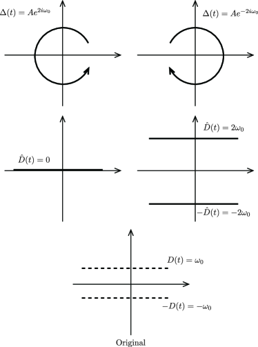
Figure 1: Top: rotation of the off-diagonal elements. Middle: New states of $\hat{H}$. Bottom: The original states of $H$. In this case, the resonance is possible only for the anti-clockwise rotation.

Although this model is very useful for understanding the origin of the asymmetry, there is a problem in defining the number density. In this model, there is no non-perturbative transition (i.e, the Stokes phenomena) between the “adiabatic states”. On the other hand, the adiabatic states cannot keep diagonalizing the Hamiltonian, which causes oscillation of the number density. To avoid such problem, one has to define the creation and the annihilation operators for the asymptotic states, but in this model the asymptotic states are not defined.. To introduce a non-adiabatic transition, we have to extend the model.

II.3 Majorana fermion with linear time-dependence ($\Delta=sg(\epsilon+ivt),D=-s|\bm{k}|$)

For the cosmological preheating scenario, particle production near the enhanced symmetry point(ESP) with $\phi(t)=\epsilon+ivt$ is very important. Using the generation of the asymmetry, we also explain the crucial discrepancy between the conventional WKB expansion and the EWKB.

We start with the decoupled equation

$$\ddot{\hat{X}} + \left[\frac{g^{2}\left(\epsilon^{2}+v^{2}t^{2}\right)+|\bm{k}|^{2}}{\hbar^{2}}+\frac{s|\bm{k}|v}{\hbar(\epsilon-ivt)}\right.$$ (100)

$$\left.+\frac{3v^{2}}{4(\epsilon-ivt)^{2}}\right]\hat{X}=0.$$

Naively for the EWKB, this equation gives

$$Q_{0}(t) = -g^{2}\left(\epsilon^{2}+v^{2}t^{2}\right)-|\bm{k}|^{2}$$ (101)

and the asymmetry seems to disappear from the non-perturbative calculation. This result agrees with our numerical calculation. However, seeing the trajectory, one will find that this model has a rotational motion around the origin (i.e, the ESP). Is it true that the rotational asymmetry considered in Sec.II.2 disappears in this model? If the asymmetry disappears, what is the crucial condition?

To understand more about the situation, we show the naive Stokes lines in Fig.2, which have a double pole at $t=-i\epsilon/v$ and four turning points. Seeing the Stokes lines, one can understand the situation. The EWKB stokes lines appear after gluing the double pole and two turning points together at the origin. In this limit (i.e, $\hbar\rightarrow 0$), the stokes lines give the simple “scattering problem with an inverted quadratic potential”Enomoto:2020xlf .

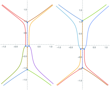
Figure 2: Stokes lines for $\epsilon=0.1,v=1,k=1,\hbar=0.1,g=1,s=\pm 1$ are given for $Q_{0}+Q_{1}$, not for $Q_{0}$. One can see four turning points (circle) and a double pole (triangle) near the origin, which are asymmetric, but they disappear in the EWKB.

Alternatively, using the numerical calculation explained in Appendix C, we find that the net number $n_{k}^{+}-n_{k}^{-}$ cannot evolve in the straight motion $\ddot{m}_{R}=0$ as long as the initial state begins with the zero particle state. In reality, however, the backreaction is important since the particle production is significant in this model, and its backreaction can bend the trajectory to give $\ddot{m}_{R}\neq 0$..

Therefore, without considering the backreaction, this model cannot generate asymmetry, but the particle production always introduces the backreaction, which is required for the asymmetry. Therefore, in reality, the asymmetry production cannot be neglected in this model.

Below, we mainly consider only the rotational motion of the off-diagonal elements, which depends only on the phase $\theta(t)$. In such models, the Landau-Zener transition is very useful. We are using the EWKB to support the analysis.

II.4 Majorana fermion with time-dependent mass (perturbative expansion)

We consider perturbative expansion of the model considered in Sec.II.2, which is given by

$$\Delta = Ae^{i\theta}\simeq A(1+i\theta+...),$$ (102)

where $\theta(t)=\omega t$ is the simplest example. The expansion is valid only for $\theta\ll 1$. Alternatively, one can choose $\theta(t)=A\cos\omega t$ with $A\ll 1$.

Reflecting on the calculation above, the above perturbative expansion might have changed the mechanism of the non-perturbative process. The significant discrepancy appears when $\theta=\omega t$. Indeed, the original theory does not allow non-adiabatic transition, while in the perturbed theory the transition is solved as the quantum scattering by a potential (after decoupling the equations). Therefore, in this example, one has to conclude that the essential mechanism of the transition has been changed by taking the perturbative expansion. In the light of the EWKB, this is because the structure of the Stokes lines, which determines the transfer matrix, is changed by the perturbation. Therefore, to avoid such discrepancy, one has to consider the expansion that does not change the essential property of the Stokes lines. We show some typical examples in appendixB.

If the particle production is the Landau-Zener type, one has to check first the global structure of the Stokes lines of the EWKB, and the local (linear) expansion has to be taken around the points where the Stokes lines cross the real-time axis. Indeed, the original Landau-Zener model considers local expansion around the state-crossing point, where the global structure of the Stokes lines has the separable form of the MTP(Merged pair of simple Turning Points). In this paper, we often consider similar expansion. Note however that the particle production is not always explained by the Landau-Zener type transition.

We sometimes compare the Landau-Zener type calculation with the EWKB Stokes lines. In our analysis, the Landau-Zener type transition is very useful for understanding the asymmetry.

II.5 Majorana fermion with time-dependent mass (The EWKB for $\Delta(t)=m_{0}e^{i\theta}$, $\theta(t)\equiv A\cos(\omega_{a}t/\hbar)$)

In this section, we consider

$$\theta(t) \equiv A\cos(\omega_{a}t/\hbar)$$

$$\Delta(t) = m_{0}e^{-i\theta}$$ (103)

and draw the Stokes lines of Eq.(82). Note that

$$\frac{\dot{\Delta}^{*}}{\Delta^{*}} = i\dot{\theta}$$

$$= \frac{i\omega_{a}}{\hbar}\sin\left(\frac{\omega_{a}t}{\hbar}\right)$$

$$\sim O(\hbar^{-1})$$ (105)

is important for the EWKB calculation.

What is important for the asymmetry is the term proportional to $s$. Terms proportional to $\dot{D}$ will disappear since $D$ is constant. Therefore, the s-dependence comes from the factor

$$-iD\frac{\dot{\Delta}^{*}}{\hbar\Delta^{*}} = -\frac{i(-s|\bm{k}|)}{\hbar}\frac{i\omega_{a}}{\hbar}\sin\left(\frac{\omega_{a}t}{\hbar}\right)$$ (106)

$$= -\frac{s|\bm{k}|\omega_{a}}{\hbar^{2}}\sin\left(\frac{\omega_{a}t}{\hbar}\right).$$

This term is suppressed in the non-relativistic limit ($|\bm{k}|\rightarrow 0$). Therefore, the asymmetry is not significant in the non-relativistic limit. This result may not be consistent with the intuition, since in the non-relativistic limit, violation of the helicity could be significant. We will explain the reason later in this section.

To understand more about the origin of the asymmetry, we have calculated the Stokes lines for typical $Q_{0}$, which is shown in Fig.3 together with their “potentials”. We have excluded the imaginary part for simplicity. See Appendix B for more details.

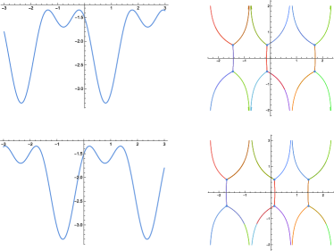
Figure 3: The Stokes lines and the potential are shown for $Q(t)=-1.5-s0.8\sin(2t)-\sin^{2}(2t)$ and $V(t)=-s0.8\sin(2t)-\sin^{2}(2t)$. The upper is for $s=+1$ and the lower is for $s=-1$.

Seeing Fig.3 and the solutions of $Q_{0}=0$, one can understand that the basic structures of the MTPs are completely the same but their positions are shifted by changing the sign of $s$. Therefore, for an eternal oscillation, the production becomes symmetric on average, but for a damped oscillation, the asymmetry appears because the particle production is not simultaneous for different $s=\pm 1$. The time-dependent amplitude of the oscillation generates different number densities at each MTP. The asymmetry is therefore determined by the time-dependence of the amplitude. Particle production is exclusive at each MTP

One thing that has to be clarified is the vanishing asymmetry in the limit of $|{\bm{k}}|\rightarrow 0$. This phenomenon can be understood easily by considering the original equation (Landau-Zener type). In Fig.4, we show the motion of the two states for $\hat{H}$. In the left, $s=\pm 1$ states are distinguishable when $|{\bm{k}}|\neq 0$, while in the right, $s=\pm 1$ states are not distinguishable when $|{\bm{k}}|=0$. Simultaneous particle production is possible only when $k=0$, which corresponds to vanishing asymmetry.

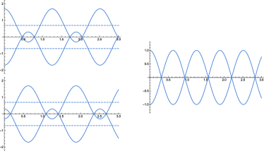
Figure 4: After using Eq.(II.1), the time-dependence appears only in the diagonal elements. Left: As far as $|\bm{k}|\neq 0$, one can discriminate $s=1$ and $s=-1$. Right: For $|\bm{k}|=0$, particle production cannot discriminate the helicity.

One can compare the above result with the earlier calculation given in Ref.Dolgov:1996qq ; Enomoto:2018yeu . In Ref.Dolgov:1996qq , perturbative expansion has been used to expand $e^{i\theta}$ to calculate non-perturbative particle production, where the asymmetry appears from the interference between terms. In our analysis, the asymmetry appears because the particle production is exclusive.

In Ref.Enomoto:2018yeu , it has been shown for a single Dirac fermion that crucial cancellation disturbs asymmetry production. The reason is very simple. For a single Dirac fermion, the complex mass has to be introduced as

$$m_{D}\overline{\psi_{L}}\psi_{R}+m_{D}^{*}\overline{\psi_{R}}\psi_{L},$$ (107)

which flips the rotational direction by the exchange $L\leftrightarrow R$. More precisely, since the exchange $L\leftrightarrow R$ inverses the rotational motion of the complex Dirac mass, “matter production” of the left-handed fermion occurs simultaneously with “antimatter production” of the right-handed fermion, and vice versa. To avoid this cancellation, one has to introduce more than two Dirac fermions, whose off-diagonal elements (interaction) is given by

$$\left[m_{\Delta}(\overline{\psi_{Lj}}\psi_{Ri}+\overline{\psi_{Rj}}\psi_{Li})+h.c.\right].$$ (108)

or

$$\left[m_{\Delta}\overline{\psi_{Lj}}\psi_{Ri}+h.c.\right].$$ (109)

We will go back to this topic in Sec.III.

II.6 Majorana fermion with time-dependent mass ($\theta(t)=A/(1+e^{-at/\hbar})$)

In this section, we consider the simple rotational motion of the phase. As we will see later in this section, the model clearly describes the origin of the asymmetry in particle production. We consider

$$\theta(t)=\frac{A}{1+e^{-at/\hbar}},$$ (110)

which gives transition of the phase from $\theta_{i}=0$ to $\theta_{e}=A$ around $t=0$. We showed the motion of $\theta(t)$ and $\dot{\theta}(t)$ in Fig.5.

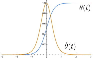
Figure 5: $\theta(t)$ and $\dot{\theta}(t)$ for $\theta(t)=A/(1+e^{-at/\hbar})$

We take

$$m_{R}(t) = g\varphi(t)\equiv g\varphi_{0}e^{i\theta(t)}$$

$$\theta(t) \equiv \frac{A}{1+e^{-at/\hbar}},$$ (111)

where $\varphi_{0}$ is real. Again, one can remove the time-dependence of the off-diagonal elements using the translation

$$\hat{\Psi} \equiv U_{T}^{-1}\Psi,$$

$$U_{T} \equiv \left(\begin{array}[]{cc}e^{i\theta(t)/2}&0\\ 0&e^{-i\theta(t)/2}\end{array}\right).$$ (114)

The Hamiltonian after the transformation becomes

$$\hat{H} \equiv U_{T}^{-1}HU_{T}-iU_{T}^{-1}\dot{U}_{T}$$ (117)

$$= \left(\begin{array}[]{cc}-s|\bm{k}|-\frac{1}{2}\hbar\dot{\theta}&sg\varphi_{0}\\ sg^{*}\varphi_{0}&s|\bm{k}|+\frac{1}{2}\hbar\dot{\theta}\end{array}\right).$$

Note that the new terms in the diagonal elements do not have “$s$” in their coefficients.

The new Hamiltonian is quite useful for our discussion. One can see in Fig.6 that the new term ($\propto\dot{\theta}$) makes a bump around $t=0$ and the intersection (in the sense of the original Landau-Zener model) appears only for $s=-1$, because of the signs in front of $\dot{\theta}$. This means that for a certain range of $k$, only $s=-1$ particles can experience the Landau-Zener type transition. The particle production seems exclusive in this case, at least for the Landau-Zener type particle production.

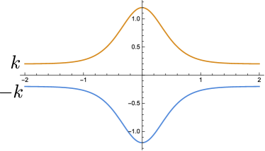
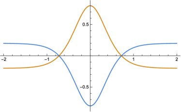
Figure 6: Upper: Time-dependence of the diagonal elements of $\hat{H}$ for $s=+1$ and $k\neq 0$, in which one can see no crossing. Lower: Time-dependence of the diagonal elements of $\hat{H}$ for $s=-1$ and $k\neq 0$, in which each state crossing causes Landau-Zener transition.

In this model, one can see state crossing of $s=-1$ for $k<k_{*}\equiv\frac{aA}{8}$. Since $A$ defines the amplitude of $\theta(t)$, we found $n\propto k_{*}^{3}\propto A^{3}$ in this model, which supports the claim given in Ref.Dolgov:1996qq .

Considering the original Landau-Zener model, the probability of the transition (i.e, the magnitude of the particle production) is determined by the velocity at each crossing point ($t_{1,2}$), which is

$$\frac{|g\varphi_{0}|^{2}}{v(t_{i})} < 1$$ (118)

$$v(t_{i}) \equiv \dot{\hat{D}}(t_{i})\equiv\hbar\frac{\ddot{\theta}(t_{i})}{2}.$$ (119)

Note that in this formulation, $k$-dependence is appearing in $t_{i}$.

In this argument, the radius of the Fermi sphere is important for estimating the number density. For large $k$, the top of the two bumps meet at

$$k_{*} \equiv \frac{aA}{8},$$ (120)

where the velocity of the state becomes $\ddot{\theta}\simeq 0$. See the Fig.7. Here the conventional Landau-Zener model, which uses the linear expansion at the state-crossing point, does not give the correct answer.

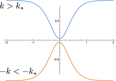
Figure 7: The upper and the lower states start to fall apart for larger $|k|$, and the crossing disappears near $k\sim k_{*}$. At this moment $\ddot{\theta}$ disappears and higher calculation becomes importantEnomoto:2020xlf .

The transition of this kind has already been calculated in Ref.Enomoto:2020xlf , in which the scattering problem with an inverted quartic potential has been considered. Near the top of the bumps, we considered in Ref.Enomoto:2020xlf the equation given by

$$i\hbar\frac{d}{dt}\left(\begin{array}[]{c}\psi_{1}\\ \psi_{2}\end{array}\right) = \left(\begin{array}[]{cc}-(at^{2}+\epsilon)&\Delta\\ \Delta&at^{2}+\epsilon\end{array}\right)\left(\begin{array}[]{c}\psi_{1}\\ \psi_{2}\end{array}\right),$$ (127)

which gives after decoupling the following equation

$$\left[\hbar^{2}\frac{d^{2}}{dt^{2}}+\left(\Delta^{2}-i(2at)\hbar\right)+\left(at^{2}+\epsilon\right)^{2}\right]\psi_{1} = 0.$$ (128)

In terms of the EWKB, $Q_{0}$ of the equation is

$$Q_{0} = -\Delta^{2}-\left(at^{2}+\epsilon\right)^{2},$$ (129)

where the “potential” is

$$V(t) = -a^{2}t^{4}-2a\epsilon t^{2}<0$$ (130)

and the “energy” is $E=\Delta^{2}+\epsilon^{2}>0$. We thus find

$$Q_{0}(t) = -\Delta^{2}-\epsilon^{2}-a^{2}t^{4}-2a\epsilon t^{2}.$$ (131)

For the model considered in this section, we have

$$\dot{\theta}(t) \simeq 2k_{*}+\frac{1}{2}\dddot{\theta}(0)t^{2}+...$$ (132)

$$\dddot{\theta}(0) \equiv -4a_{2},$$ (133)

which gives the Hamiltonian for $s=-1$

$$\hat{H} = \left(\begin{array}[]{cc}\Delta k+a_{2}t^{2}&-g\varphi_{0}\\ -g^{*}\varphi_{0}&-\Delta k-a_{2}t^{2}\end{array}\right),$$ (136)

where we introduced $\Delta k\equiv|k|-k_{*}$ . There is no state crossing for $|k|>k_{*}$($\Delta k>0$), but to solve the scattering problem of the quartic potential, one can see that the transition can be significant yetEnomoto:2020xlf . Transforming the above equation into $Q(x)=-\kappa_{4}-x^{4}$, one can easily find that $\kappa_{4}$ in the equation gives the bound $\kappa_{4}\lesssim 1$, which determines the radius of the Fermi sphere.

Although rather crude, one can see that when the tops of the bumps coincide at $\Delta k=0$, the Fermi sphere can be larger than $k_{*}$ if $a\geq(g^{2}\varphi_{0}^{2}+\Delta k)^{1/2}A^{1/3}$ is satisfied. Here, $A$ represents the variation (amplitude) of $\theta(t)$ and $a$ determines the speed of the transition (or the width of the domain wall). The above condition is showing that particle production is more efficient when the variation of $\theta$ is larger and the speed of the transition is higher. This result coincides with intuition.

For $A\sim O(1)$, $a\sim g\varphi_{0}$ gives the Fermi sphere $k_{F}=k_{*}\simeq g\varphi_{0}/8$. Variation from this point will change the Fermi sphere from the naive estimation $k_{F}\sim k_{*}$.

We show our numerical results in Fig.8, which depict the shapes of the distributions (upper panel) and the time evolution of the number density for each state (lower panel). One can see clearly that $s=+1$ production is suppressed compared with $s=-1$. (Note that in the lower panel the number densities are given for the log scale.)

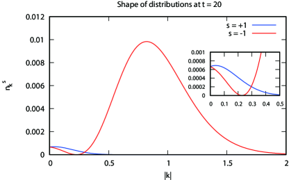
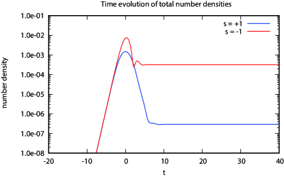
Figure 8: The results of numerical calculation with the parameters $|m_{R}|=a=1.0,A=\pi/3.$ Upper: shapes of the distributions for each helicity state after the production ($t=20$). Lower: time evolution of the number densities (log scale).

In this model, the MTP structure always appears twice during particle production. When one calculates the Fermi sphere of particle production, this double MTP structure causes a less trivial modification of the distribution, as far as the particles do not decay between the two MTPs. The typical distributions are shown in Fig.9 for $\kappa(\Delta)\propto\Delta^{2}$.

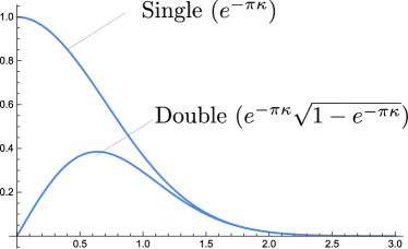
Figure 9: Typical distribution functions for $\kappa(\Delta)$ are shown for the single and the double MTP models.

Let us explain why this distribution is very important for our scenario. Since the off-diagonal elements are representing the symmetry-violating interaction, asymmetry in the $g\varphi_{0}\rightarrow 0$ limit is very important. For the Majorana fermion, since the off-diagonal elements are representing the Majorana mass, small $|\Delta|$ seems to be making the particle production easier. This speculation is true for a single MTP scenario, but for our double MTP scenario, one has to consider Fig.9 for the distribution. In the $g\varphi_{0}\rightarrow 0$ limit, the particle production vanishes as one can see from Fig.9. Therefore, a tiny interaction suppresses particle production (and asymmetry).

From the above results, one can see that static motion (always $\ddot{\theta}=0$) gives no state crossing in this model.

Although very crude, one can estimate the particle production when cosmological domain walls decay. For the typical cosmological domain wall of tension $\sigma\sim\Lambda^{3}$ and width $\delta_{w}\sim\Lambda^{-1}$ decaying at the density $\rho\sim\sigma^{2}/M_{p}^{2}$, the number density of the produced particle can be estimated as $k_{F}\sim 0.1\Lambda$ for fast-moving wall. However, since efficient particle production causes friction to the domain wall motion, the maximum number density should be estimated as $n\lesssim\rho/\Lambda\sim\Lambda^{5}/M_{p}^{2}$ when the temperature of the Universe is $T_{D}\sim\sqrt{\sigma/M_{p}}$. We conclude that asymmetric particle production can be efficient for typical cosmological domain walls.

III Dirac fermions

As we have mentioned previously, asymmetry will be canceled for a single Dirac fermion. Let us see more details of the cancellation mechanism. For a single Dirac fermion, one may find complex mass terms as

$$\left[m_{\Delta}\overline{\psi_{L}}\psi_{R}+m_{\Delta}^{*}\overline{\psi_{R}}\psi_{L}\right]$$ (137)

Following the strategies we have considered in this paper, one can explicitly calculate particle production for four species; left(right)-handed matter(antimatter). Our observation is very simple. Since the $L\leftrightarrow R$ exchange flips the rotational direction, one can immediately find that $L$ and $R$ productions are exclusive. Since the matter-antimatter is also exclusive, L-matter production and R-antimatter production are simultaneous. Regarding this particle production as the decay process, one can say that depending on the sign of $\dot{\theta}$, the field $\theta$ “selectively” decays into L-matter and R-antimatter (or L-antimatter and R-matter for the opposite sign). Therefore, for a single Dirac fermion, direct asymmetry production is impossible in total.

Although a single Dirac fermion is excluded for the (direct) baryogenesis, there is hope in multiple Dirac fermions. To show an example, let us consider a fictitious “lepton” $\psi^{l}$ and a “quark” $\psi^{q}$ for the calculation and suppose that each fermion is massless (i.e, we are considering a naive relativistic limit) but they have the Yukawa interaction

$$g\phi\overline{\psi^{l}}\psi^{q}+h.c$$ (138)

$$= g\phi(\overline{\psi^{l}_{R}}\psi^{q}_{L}+\overline{\psi^{l}_{L}}\psi^{q}_{R})+h.c.$$

Since in this case, the $L\leftrightarrow R$ exchange does not flip the rotational direction, $\psi^{q}_{L}$-matter production and $\psi^{q}_{R}$-matter production simultaneously occur, and they are exclusive to $\psi^{q}_{L}$-antimatter and $\psi^{q}_{R}$-antimatter production. We thus find the net baryon number from the cosmological particle production.

On the other hand, considering the $l\leftrightarrow q$ exchange, $\psi^{q}_{L,R}$-matter production is exclusive to $\psi^{l}_{L,R}$-matter production. We thus find that the negative lepton number has to be generated simultaneously with the positive baryon number, and vice versa. This result is consistent with effective charge conservation.

The trick of this baryogenesis scenario is very simple in the massless limit. If one rearranges the pairs as $\psi_{1}=(\psi_{1L},\psi_{1R})\equiv(\psi^{q}_{L},\psi^{l}_{R}$) and $\psi_{2}=(\psi_{2L},\psi_{2R})\equiv(\psi^{l}_{L},\psi^{q}_{R}$), the Yukawa interaction can be written as

$$\left[g\phi\overline{\psi^{l}_{R}}\psi^{q}_{L}+h.c.\right]+\left[g\phi\overline{\psi^{l}_{L}}\psi^{q}_{R}+h.c.\right]$$ (139)

$$= \left[g\phi\overline{\psi_{1R}}\psi_{1L}+h.c.\right]+\left[g^{*}\phi^{*}\overline{\psi_{2R}}\psi_{2L}+h.c.\right],$$

which represents the complex Dirac mass terms for two independent Dirac fermions $\psi_{1,2}$. In the original $\psi^{q}$ and $\psi^{l}$, the “exclusive pairs” are rearranged to avoid the cancellation of the net B and L numbers.

Remember that in the previous (Majorana) models, asymmetry vanishes for $\bm{k}\rightarrow 0$. Therefore, we are going to discuss the non-relativistic limit, where the original mass terms

$$m_{q}\overline{\psi^{q}}\psi^{q}-m_{l}\overline{\psi^{l}}\psi^{l}$$ (140)

are not negligible but $\bm{k}\simeq 0$ is negligible for both fermions. Here, the minus sign in front of $m_{l}$ is for later convenience. We also assume $m_{q}\simeq m_{l}$ for simplicity.

First, consider the conventional decomposition

$$\psi = \int\frac{d^{3}k}{(2\pi)^{3}}e^{-i\bm{k}\cdot\bm{x}}\sum_{s}\left[u^{s}_{\bm{k}}(t)a^{s}_{\bm{k}}+v^{s}_{\bm{k}}(t)b^{s\dagger}_{-\bm{k}}\right]$$ (141)

and the single-field Dirac equation

$$(i\not{\partial}-m_{D})\psi = 0.$$ (142)

Carefully following the formalism given in Ref.Peloso:2000hy , one will find

$$\dot{u}_{\pm} = iku_{\mp}\mp im_{D}u_{\pm},$$ (143)

which can be written in the matrix as

$$i\frac{d}{dt}\left(\begin{array}[]{c}u_{+}\\ u_{-}\end{array}\right) = \left(\begin{array}[]{cc}m_{D}&-k\\ -k&-m_{D}\end{array}\right)\left(\begin{array}[]{c}u_{+}\\ u_{-}\end{array}\right).$$ (150)

Diagonalizing this equation for constant matrix elements, one will find the adiabatic states (the WKB solutions) as

$$i\frac{d}{dt}\left(\begin{array}[]{c}\tilde{u}_{+}\\ \tilde{u}_{-}\end{array}\right) = \left(\begin{array}[]{cc}\sqrt{m_{D}^{2}+k^{2}}&0\\ 0&-\sqrt{m_{D}^{2}+k^{2}}\end{array}\right)\left(\begin{array}[]{c}\tilde{u}_{+}\\ \tilde{u}_{-}\end{array}\right).$$ (157)

The original $u_{\pm}$ and $\tilde{u}_{\pm}$ coincides at $k\sim 0$.

Let us introduce the interaction given in Eq.(138) and take $\bm{k}\rightarrow 0$. Assuming $m_{q}$ and $m_{l}$ are constant, we find

$$i\frac{d}{dt}\left(\begin{array}[]{c}u_{+}^{q}\\ u_{+}^{l}\end{array}\right) = \left(\begin{array}[]{cc}m_{q}&m_{\Delta}^{*}\\ m_{\Delta}&-m_{l}\end{array}\right)\left(\begin{array}[]{c}u_{+}^{q}\\ u_{+}^{l}\end{array}\right).$$ (165)

and

$$i\frac{d}{dt}\left(\begin{array}[]{c}u_{-}^{q}\\ u_{-}^{l}\end{array}\right) = \left(\begin{array}[]{cc}-m_{q}&-m_{\Delta}^{*}\\ -m_{\Delta}&+m_{l}\end{array}\right)\left(\begin{array}[]{c}u_{-}^{q}\\ u_{-}^{l}\end{array}\right).$$ (172)

At this moment, the cancellation could not be clear from the above equations.

Decoupling the equations, we find

$$\ddot{u}_{+}^{q}+\left[-\frac{\dot{m}_{\Delta}^{*}}{m_{\Delta}^{*}}+i(m_{q}-m_{l})\right]\dot{u}_{+}^{q}$$

$$+\left[|m_{\Delta}|^{2}+m_{q}m_{l}-i\frac{\dot{m}_{\Delta}^{*}}{m_{\Delta}^{*}}m_{q}\right]u_{+}^{q} = 0$$ (173)

Redefining the interaction as $m_{\Delta}=m_{0}e^{i\theta(t)}$, we have

$$\frac{\dot{m}_{\Delta}^{*}}{m_{\Delta}^{*}} = -i\dot{\theta}.$$ (174)

Also defining $\delta M\equiv m_{q}-m_{l}\geq 0$, the equation becomes

$$\ddot{u}_{+}^{q}+i\left[\dot{\theta}+\delta M\right]\dot{u}_{1+}$$

$$+\left[|m_{\Delta}|^{2}+m_{q}m_{l}-\dot{\theta}m_{q}\right]u_{+}^{q}=0$$ (175)

The standard form of the EWKB will be obtained using

$$\hat{u}_{+}^{q} \equiv \exp\left(\frac{i}{2}\int^{t}\left[\dot{\theta}+\delta M\right]dt\right)u_{+}^{q}.$$ (176)

This also removes the time-dependence of the off-diagonal elements of the Landau-Zener formalism. Finally, we have

$$\ddot{\hat{u}}_{+}^{q}+\left[-\frac{i}{2}\ddot{\theta}+\frac{3(\dot{\theta}+\delta M)^{2}}{4}\right.$$ (177)

$$\left.+m_{0}^{2}+m_{l}m_{q}-\dot{\theta}m_{q}\right]u_{+}^{q}$$

$$= 0.$$

It seems difficult to understand the situation from the decoupled equations. Therefore, we are going back to the original matrix form.

If Eq.(176) has been applied to Eq.(165), one will find

$$i\frac{d}{dt}\left(\begin{array}[]{c}\hat{u}_{+}^{q}\\ \hat{u}_{+}^{l}\end{array}\right) = \left(\begin{array}[]{cc}\frac{M_{1/2}-\dot{\theta}}{2}&m_{0}\\ m_{0}&-\frac{M_{1/2}-\dot{\theta}}{2}\end{array}\right)\left(\begin{array}[]{c}\hat{u}_{+}^{q}\\ \hat{u}_{+}^{l}\end{array}\right),$$ (184)

and

$$i\frac{d}{dt}\left(\begin{array}[]{c}\hat{u}_{-}^{q}\\ \hat{u}_{-}^{l}\end{array}\right) = \left(\begin{array}[]{cc}-\frac{M_{1/2}+\dot{\theta}}{2}&-m_{0}\\ -m_{0}&\frac{M_{1/2}+\dot{\theta}}{2}\end{array}\right)\left(\begin{array}[]{c}\hat{u}_{-}^{q}\\ \hat{u}_{-}^{l}\end{array}\right),$$ (191)

where $M_{1/2}\equiv(m_{q}+m_{l})/2$. This form is very familiar in this paper. From the above equations, we found that the situation is quite similar to the single Dirac fermion, and the matter-antimatter asymmetry is indeed canceled (i.e, net baryon and lepton numbers vanish) in the non-relativistic limit.

For completeness, let us consider a generalization of the scenario. Since the left-handed and the right-handed fermions are independent particles, one can also consider the Yukawa interactions written as

$$\left[m_{\Delta ij}\overline{\psi_{Lj}}\psi_{Ri}+h.c.\right]+\left[m_{\Delta ji}\overline{\psi_{Li}}\psi_{Rj}+h.c.\right],$$ (192)

where $m_{\Delta ij}\neq m_{\Delta ji}$ is possible.

IV Conclusions and discussions

As we have seen explicitly, the origin of the asymmetry in the particle production from the rotational motion is essentially the exclusive particle production. This property has been found by using the Landau-Zener model and the EWKB Stokes lines for the decoupled equations. We also pointed out that the perturbative expansion may sometimes change the Stokes lines. To avoid such discrepancy, one has to draw the Stokes lines of the original theory first and consider perturbation at the points where the Stokes lines cross the real-time axis. For the Dirac fermion, because of the left and right-handed components, the total asymmetry cancels for the single-field model. For the multiple Dirac fermions, we have seen that cancellation can be avoided in the relativistic limit. In all cases, the asymmetry vanishes for $k\rightarrow 0$.

Perturbative expansion is sometimes used before non-perturbative calculation. Our concern was that such simplification may change the structure of the Stokes lines of the original theory and the theory after perturbative expansion cannot reproduce the physics of the original theory. For physics, the two theories could not always be needed to be identical, but the difference has to be under control. To avoid the problem, one has to draw first the Stokes line of the original theory to find a separable structure of the Stokes lines, where local expansion is applicable. Indeed, the idea described in Zener’s original paperZener:1932ws follows this regulation. This strategy is crucial for a damped oscillation, as is shown in Fig.3.

We started with the simplest example (i.e, simple rotation $\Delta(t)=Ae^{i\omega_{0}t}$), and carefully examined the essential mechanism of the asymmetry production for typical situations, comparing the structure of the Stokes lines and the original equations.

V Acknowledgment

The authors would like to thank Nobuhiro Maekawa for collaboration in the very early stages of this work. SE was supported by the Sun Yat-sen University Science Foundation.

Appendix A A short introduction to the EWKB and the Borel resummation

As we have mentioned in the introduction of this paper and in our previous paperEnomoto:2020xlf , there has been many papers in which the Stokes phenomena is used to study particle production. However, we feel that the crucial difference between the conventional WKB approximation and the exact WKB is not well understood widely.

First, the conventional WKB approximation generically gives a divergent power series, while the EWKB considers the Borel resummation to control the WKB expansion.

Second, the following misinterpretation could arise. Since the above situation is drastically improved by taking the Borel resummation, one might naively think that the conventional WKB is certificated by the EWKB, and there is no crucial diference at the end. This speculation is sometimes very dangerous.

The discrepancy will be obvious when $Q(x)$ of the “Schrödinger equation”

$$\left[-\frac{d^{2}}{dx^{2}}+\eta^{2}Q(x)\right]\psi(x,\eta) = 0,$$ (193)

is replaced by $Q(x,\eta)$. In this case, the discussion of the stokes phenomena becomes quite vague (or at most very complicated) for the conventional WKBBerry:1972na .

Now remember the model discussed in Sec.II.3. Although both our numerical calculation and the perturbative calculation of Ref.Dolgov:1996qq are giving the correct answer, it would be difficult for the conventional WKB to explain why the asymmetry of the Stokes lines disappears for finite $\hbar$. Using the EWKB, one can easily understand that the Stokes lines have to be calculated for $S_{-1}$, where $S_{-1}$ is the coefficient of $\eta$ of the WKB expansion. For the conventional WKB, the asymmetry of the Stokes lines seems to disappear only in the limit $\hbar\rightarrow 0$, and something other than the conventional WKB is required to explain the situation.

In the followings, we show explicitly what determines the Stokes phenomena in the EWKB and why the Borel resummation is crucial for the calculation.

A.1 What is the Borel resummation?

Let us solve the very simple Ordinary Differential Equation(ODE)

$$z^{2}\frac{du}{dz} = -u+z,\,\,\,u(0)=1$$ (194)

using expansion into power series

$$u(z) = \sum_{n=0}^{\infty}u_{n}z^{n}.$$ (195)

One can find the solution

$$u(z) = \sum_{n=0}^{\infty}(-1)^{n}n!z^{n}+1,$$ (196)

but this is a divergent power series because of the factor $n!$. To remedy the situation, we note that the Laplace transformation of a function $f$

$$(Lf)(t) = \int^{\infty}_{0}e^{-t\tau}f(\tau)d\tau$$ (197)

gives (after partial integration)

$$L\left[\frac{df}{d\tau}\right] = t(Lf)-f(0),$$ (198)

which can be applied to $f=\tau^{n}/n!$ to give

$$L\left[\frac{\tau^{n}}{n!}\right] = t^{-(n+1)}.$$ (199)

Since the factor $1/n!$ arises in this formula, it would be natural to expect that after using the inverse Laplace transformation, the factor $n!$ of the divergent power series can be removed. This speculation is correct.

Replacing $z$ by $t\equiv 1/z$, and after executing the inverse Laplace transformation, one will find

$$(L^{-1}u)(\tau) = \sum_{n=0}^{\infty}(-1)^{n}n!\left(\frac{\tau^{n}}{n!}\right)$$ (200)

$$= \frac{1}{1+\tau}.$$

After the Laplace transformation, the original power series can be written by the integral

$$u_{B}(z) = \int^{\infty}_{0}e^{-\tau/z}\left(\frac{1}{1+\tau}\right)d\tau.$$ (201)

This is the basic strategy of the Borel resummation. After defining $s\equiv\tau/z$, $U(z)$ is given by a simpler form

$$u_{B}(z) = \int^{\infty}_{0}e^{-s}\left(\frac{1}{s+z^{-1}}\right)ds.$$ (202)

If the pole at $s=z^{-1}$ moves around the origin, it crosses the integration contour and picks up a residue to give an additional contribution $2\pi ie^{1/z}$ (the Stokes phenomena).

Application of this simple idea to the WKB expansion is not so much simple but the calculation is straight. Let us see what happens in the WKB expansion and how one can understand the origin of the Stokes phenomena in terms of the Borel resummation.

A.2 The Borel resummation for the WKB expansion

Our starting point is the “Schrödinger equation” in quantum mechanics given by

$$\left[-\frac{d^{2}}{dx^{2}}+\eta^{2}Q(x,\eta)\right]\psi(x,\eta) = 0,$$ (203)

where

$$Q(x,\eta) = V-E$$ (204)

for the potential $V$ and the energy $E$. Just for simplicity, we assume that $Q$ is given by

$$Q(x,\eta)=\sum_{k=0}^{\infty}\eta^{-2k}Q_{2k}(x),$$ (205)

which simplifies the calculation as is shown in Eq.(214) later.

Assuming that the solution $\psi$ is written by $\psi(x,\eta)=e^{R(x,\eta)}$, one will have

$$\psi = e^{\int^{x}_{x_{0}}S(x,\eta)dx}$$ (206)

for $S(x,\eta)\equiv\partial R/\partial x$. We have the condition for $S$ given by

$$-\left(S^{2}+\frac{\partial S}{\partial x}\right)+\eta^{2}Q = 0.$$ (207)

Expanding $S$ as $S(x,\eta)=\sum_{n=-1}^{n=\infty}\eta^{-n}S_{n}$, one will have

$$S=\eta S_{-1}(x)+S_{0}(x)+\eta^{-1}S_{1}(x)+...,$$ (208)

which gives

$$S_{-1}^{2} = Q_{0}$$ (209)

and

$$2S_{-1}S_{2j} = -\left[\sum_{k\geq 0}^{j}S_{2k}S_{2(j-k)-1}+\sum_{k\geq 0}^{j-1}S_{2k+1}S_{2(j-k-1)}\right.$$ (210)

$$\qquad\left.+\frac{dS_{2j-1}}{dx}\right]$$

$$2S_{-1}S_{2j+1} = -\left[\sum_{k\geq 0}^{j}S_{2k}S_{2(j-k)}+\sum_{k\geq 0}^{j-1}S_{2k+1}S_{2(j-k)-1}\right.$$ (211)

$$\qquad\left.+\frac{dS_{2j}}{dx}-Q_{2(j+1)}\right]$$

for $j\geq 0$. Note that the sign dependence of $S_{-1}=\pm\sqrt{Q_{0}}$ reflects to the odd terms as $\pm S_{2j+1}$ but not to the even terms. Using this relation, one will have a simpler form

$$\psi = \frac{1}{\sqrt{S_{odd}}}e^{\int^{x}_{x_{0}}S_{odd}dx}$$ (213)

$$S_{odd}\equiv\sum_{j\geq 0}\eta^{1-2j}S_{2j-1}.$$

Depending on the sign of the first $S_{-1}$, there are two solutions $\psi_{\pm}$, which are given by

$$\psi_{\pm} = \frac{1}{\sqrt{S_{odd}}}\exp\left(\pm\int^{x}_{x_{0}}S_{odd}dx\right).$$ (214)

The above WKB expansion is usually divergent.

Let us consider the Borel resummation for the WKB expansion. Since $x$ appears in the coefficients of the $\eta$ expansion, we consider the Borel resummation for $\eta$, not for $x$. Note that this point is different from the simplest example discussed in the previous section. We thus have

$$\psi_{\pm} \rightarrow \Psi_{\pm}\equiv\int^{\infty}_{\mp s(x)}e^{-y\eta}\psi_{\pm}^{B}(x,y)dy,$$ (216)

$$s(x)\equiv\int^{x}_{x_{0}}S_{-1}(x)dx,$$

where the $y$-integral is parallel to the real axis. What is important here for the Stokes phenomena is that the starting point of the integration is naturally moved from the origin to $s(x)$ due to $S_{-1}\eta$ and $y\eta$ in the exponent. Now the starting points of the integration paths depend explicitly on the original coordinate $x$. See Fig.(10) for more information about the contour and the Stokes phenomena.

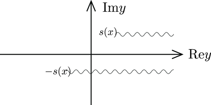
Figure 10: The wavy lines are the paths of integration in the Borel resummation. Since the paths overlap when $\mathrm{Im}[s]=0$, the Stokes phenomena appears if one crosses the Stokes lines defined by $\mathrm{Im}[s]=0$.

Therefore, one can easily expect that if one moves in the complex $x$ space, the integration contour may cause the Stokes phenomena similar to the one discussed in the previous section.

See also the simplest example in Sec.II.3, which clearly explains why EWKB is useful.

Locally, the Stokes phenomenon around the turning points ($Q=0$) can also be explained by using the Airy function ($Q(x)=x$). However, to generalize the discussion, the technique of the Borel resummation seems to be inevitable.

Appendix B The Exact WKB for cosmological particle production

In this appendix, we show the calculation of cosmological particle production in the light of the Exact WKB. We show explicitly the Stokes lines for bosonic and fermionic preheating and examine the adequacy of the conventional linear approximation at the enhanced symmetry point (ESP). After the linear approximation, which is local, the connection formula at that point is identical to the scattering problem by an inverted quadratic potential (for bosonic preheating) or the Landau-Zener transition (for fermionic preheating), whose Stokes lines are given by the Merged pair of simple Turning Points(MTP). If the imaginary part of $Q_{0}$ remains, the MTP is unmerged.

The Stokes lines in this appendix are drawn by using MathematicaMathematica-stokes .

B.1 Bosonic preheating

We first review the standard calculation based on the special function and then explain the EWKB calculation.

B.1.1 Standard calculation : Exact local solution after linear approximation, $m(t)\rightarrow m(t_{i})+\dot{m}(t_{i})(t-t_{i})$

Just after inflation, the motion of the inflaton field is usually a damped oscillation, whose particle production cannot be solved exactly. However, at least near the center of the oscillation, or very close to the ESP where particle production is likely to take place, the linear approximation can be made with respect to $t$. We are going to review the local solution obtained from the linear approximation at the ESP.

One can rewrite the inflaton motion as $\phi(t)=\phi(t_{i})+\dot{\phi}(t_{i})(t-t_{i})$, where $t_{i}$ is the $i$-th minimum of $m^{2}(t)$. Typically, the mass of a scalar field (e.g, $\chi$) is given by

$$m^{2}_{\chi}(t) = m_{0}^{2}+g^{2}_{2}\phi(t)^{2},$$ (217)

where $\phi(t)$ is the oscillating inflaton field. If we consider the Lagrangian

$${\cal L}_{\chi} = \frac{1}{2}\partial_{\mu}\chi\partial^{\mu}\chi-\frac{1}{2}m_{0}^{2}\chi^{2}-\frac{1}{2}g_{2}^{2}\phi(t)^{2}\chi^{2},$$ (218)

the equation of motion is

$$\frac{d^{2}\chi}{dt^{2}}+\left[k^{2}+m^{2}_{\chi}(t)\right]\chi=0.$$ (219)

If one replaces $\phi(t)$ with $\phi(t)\simeq vt$, the equation is equivalent to the Schrödinger equation with the “inverted quadratic potential”. Then the connection formula is obtained by solving the quantum scattering problem. The “potential” is given by

$$V(t) = -\left(g_{2}^{2}v^{2}\right)t^{2},$$ (220)

where the corresponding “energy” is

$$E = k^{2}+m_{0}^{2}.$$ (221)

Since $E>V$ is always true in this case, there is no classical turning point of the scattering problem. Here we have neglected the expansion of the Universe, which can be introduced by making redefinitions of the parameters.

Typically, the WKB expansion is used to find

$$\chi_{k}(t) = \frac{\alpha_{k}(t)}{\sqrt{2\omega_{k}}}e^{-i\int^{t}\omega dt}+\frac{\beta_{k}(t)}{\sqrt{2\omega}}e^{+i\int^{t}\omega dt},$$ (222)

where

$$\omega_{k}(t) \equiv k^{2}+m_{\chi}^{2}(t).$$ (223)

We take $\alpha_{k}=1,\beta_{k}=0$ for the initial vacuum state. The distribution of the particle in the final state is

$$n_{\chi}(k)=|\beta_{k}|^{2},$$ (224)

which can be found by solving the scattering problem of the corresponding Schrödinger equation. For the above model (i.e, scattering by the inverted quadratic potential), the following Weber equation

$$y^{\prime\prime}(z)+\left(\nu+\frac{1}{2}-\frac{1}{4}z^{2}\right)y(z)=0$$ (225)

has the solution $D_{\nu}(z),D_{-\nu-1}(iz)$. More specifically, one can define

$$z \equiv ie^{i\pi/4}\sqrt{2g_{2}v}t$$ (226)

in the original field equation to find

$$\frac{d^{2}\chi}{dz^{2}}+\left[\nu+\frac{1}{2}-\frac{1}{4}z^{2}\right]\chi=0.$$ (227)

Here we defined

$$\nu=\frac{k^{2}+m_{0}^{2}}{2g_{2}v}i-\frac{1}{2},$$ (228)

and for later use we define

$$\kappa \equiv \frac{k^{2}+m_{0}^{2}}{2g_{2}v}$$ (229)

and

$$\nu=i\kappa-\frac{1}{2}.$$ (230)

Here, $\kappa$ is later used to estimate the particle production. Comparing the asymptotic forms of the Weber function, one will findEnomoto:2020xlf

$$D_{\nu}(z) \simeq e^{-i\frac{g_{2}v}{2}t^{2}}e^{(i\kappa-\frac{1}{2})\left(\log(\sqrt{2g_{2}v}|t|)-i\frac{\pi}{4}\right)},$$

$$D_{-\nu-1}(iz) \simeq e^{+i\frac{g_{2}v}{2}t^{2}}e^{(-i\kappa-\frac{1}{2})\left(\log(\sqrt{2g_{2}v}|t|)+i\frac{\pi}{4}\right)}.$$

In the limit $t\rightarrow-\infty$, the above solutions are giving the $\pm$ WKB solutions of Eq.(222). Therefore, one will have in the $t\rightarrow-\infty$ limit

$$\chi_{-} \rightarrow D_{\nu}(z)$$ (232)

$$\chi_{+} \rightarrow D_{-\nu-1}(iz).$$ (233)

In the opposite $t\rightarrow+\infty$ limit, we have

$$D_{\nu}(z) \simeq e^{-i\frac{g_{2}v}{2}t^{2}}e^{(i\kappa+\frac{1}{2})\left(\log(\sqrt{2g_{2}v}t)+i\frac{3\pi}{4}\right)}$$

$$+i\frac{\sqrt{2\pi}}{\Gamma(-\nu)}e^{i\frac{g_{2}v}{2}t^{2}}e^{-\kappa\pi}e^{(-i\kappa-\frac{1}{2})\left(\log(\sqrt{2g_{2}v}t)+i\frac{3\pi}{4}\right)},$$

which shows that in the $t=+\infty$ limit the asymptotic form of the exact solution $D_{\nu}(z)$ is the mixture of the $\pm$ WKB solutions. Thus we find the exact connection formula using the special function.

In this case, the connection formula gives the Bogoliubov transformation of the WKB solutions. Finally, we obtain the connection matrix

$$\left(\begin{array}[]{c}\alpha_{k}^{+\infty}\\ \beta_{k}^{+\infty}\end{array}\right)$$ (239)

$$= \left(\begin{array}[]{cc}\sqrt{1+e^{-2\pi\kappa}}e^{i\theta_{1}}&ie^{-\pi\kappa+i\theta_{2}}\\ -ie^{-\pi\kappa-i\theta_{2}}&\sqrt{1+e^{-2\pi\kappa}}e^{-i\theta_{1}}\end{array}\right)\left(\begin{array}[]{c}\alpha_{k}^{-\infty}\\ \beta_{k}^{-\infty}\end{array}\right).$$ (244)

Here, all the phase parameters are put into $\theta_{1,2}(k)$.

B.1.2 The Exact WKB for bosonic preheating

First, we use the EWKB to find the connection formula of the local solution, which is the exact local solution of the theory after linear expansion. Then we show the global structure of the original Stokes lines and show why such a local solution is justified.

The Stokes phenomenon around the turning points can be easily understood using the Airy function ($Q(x)=x$). In this case, the Stokes lines are defined by

$$\mathrm{Im}[s(x)] = \mathrm{Im}\left[\int^{x}_{0}x^{1/2}dx\right]$$ (246)

$$= \mathrm{Im}\left[\frac{2}{3}x^{3/2}\right]=0,$$

which is shown in Fig.11.

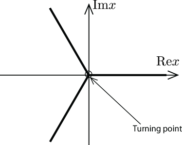
Figure 11: The Stokes lines for $Q=x$.

If $\mathrm{Re}[s(x)]>0$, $\psi_{+}$ is dominant on the Stokes line, while if $\mathrm{Re}[s(x)]<0$, $\psi_{-}$ is dominant.

When the integration paths of the Borel resummation overlap on the Stokes line, it may develop additional contributions, which is called the Stokes phenomenon. We have the following connection formulae:

• Crossing the $\psi_{+}$-Dominant Stokes line with anticlockwise rotation (seen from the turning point)

  $$\Psi_{+} \rightarrow \Psi_{+}+i\Psi_{-}$$ (247)

  $$\Psi_{-} \rightarrow \Psi_{-}$$ (248)

• Crossing the $\psi_{-}$-Dominant Stokes line with anticlockwise rotation (seen from the turning point)

  $$\Psi_{-} \rightarrow \Psi_{-}+i\Psi_{+}$$ (249)

  $$\Psi_{+} \rightarrow \Psi_{+}$$ (250)

• Inverse rotation gives a minus sign in front of $i$.

Here, we are confined to the Airy function, but generalization of this idea requires more calculationVirtual:2015HKT .

Let us use these simple formulae to solve the scattering problem by the inverted quadratic potential ($E>0$). We show the Stokes lines in Fig.12, which has a typical MTP structure.

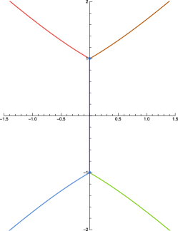
Figure 12: The Stokes lines for the inverted quadratic potential ($Q=-1-t^{2}$).

The degeneracy of the Stokes line can be solved (the MTP can be unmerged) by introducing imaginary parameters, as is explicitly shown in Fig.13. One can calculate the connection formula $1\rightarrow 2\rightarrow 3$, as is shown in Ref.Enomoto:2020xlf . One thing that is not trivial is the relation between the normalization factor and the gap, which appears when the sign of the imaginary part is changed (e.g, $E+i\epsilon\leftrightarrow E-i\epsilon$)

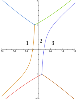
Figure 13: The Stokes lines of the MTP are unmerged by $[Q=-1-t^{2}]\rightarrow[Q=-(1+0.3i)-t^{2}]$.

For the normalization factor, we have

$$\psi_{\pm} = \frac{1}{\sqrt{S_{odd}}}\exp\left(\pm\int^{x}_{x_{0}}S_{odd}dx\right)$$ (251)

$$= \psi^{(\infty)}_{\pm}\exp\left(\pm\int^{x}_{x_{0}}\left(S_{odd}-\eta S_{-1}\right)dx\right),$$

$$\psi^{(\infty)}_{\pm} = \frac{1}{\sqrt{S_{odd}}}\exp\left(\pm\int^{x}_{x_{0}}S_{-1}dx\right)$$ (252)

$$\times\exp\left(\pm\int^{x}_{\infty}\left(S_{odd}-\eta S_{-1}\right)dx\right).$$

Among them, what is not trivial is

$$\exp\left(\pm\int^{x}_{x_{0}}\left(S_{odd}-\eta S_{-1}\right)dx\right).$$ (253)

This gives for $Q(x)=\lambda-\frac{x^{2}}{4}$,

$$2\int^{x}_{2\sqrt{\lambda}}\left(S_{odd}-\eta S_{-1}\right)dx$$ (254)

$$= \sum^{\infty}_{n=1}\frac{2^{1-2n}-1}{2n(2n-1)}B_{2n}(i\eta\lambda)^{1-2n},$$

where $B_{2n}$ is the Bernoulli number. Because of this, one has the gap given by

$$\Psi_{+}^{(\mathrm{Im}\lambda<0)} = \sqrt{1+e^{-2\pi\lambda\eta}}\Psi_{+}^{(\mathrm{Im}\lambda>0)}.$$ (255)

The calculation can be generalized to give the factor appearing on both sides of more generic MTPSilverstone:2008 ; Aoki:2009 .

From the above results, one can understand that each separable MTP structure will have the local connection matrix given by Eq.(239). This idea is very useful for calculating particle production by a damped oscillation. To understand more about the idea, we need to draw the global structure of the Stokes lines. We assume that the mass is given by $m_{\chi}(t)^{2}=g^{2}\phi(t)^{2}=g^{2}(e^{-\Gamma t}\cos(at))^{2}$. From Fig.14, one can easily understand that the linear expansion at the local minimum of $m_{\chi}^{2}$ (i.e, the local maximum of the “potential”) is giving a good approximation.

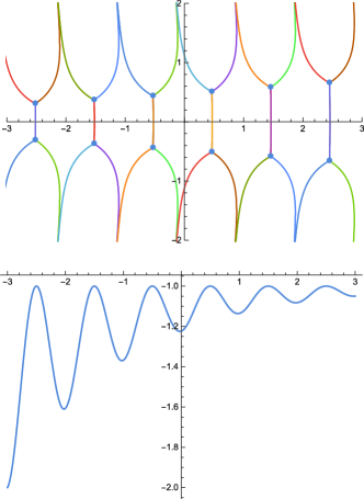
Figure 14: The Stokes lines for $Q(t)=-1-e^{-0.3(t+3)}\cos^{2}(2t)$ and a plot of $Q(t)$. Separable MTP structures are appearing at the minima of $m^{2}_{\chi}$

As we have stated above, the MTP structure is obvious in bosonic preheating. Because of the separable MTP structure, linear approximation at the ESP is easily justified and the calculation becomes local. The situation is slightly complicated for fermionic preheating.

B.2 Fermionic preheating

As we have described for bosonic preheating, we start with the local solution after linear approximation, which is nothing but the Landau-Zener model. Since the fermionic preheating with a linear $\phi(t)$ is an old idea, we carefully follow Ref.Peloso:2000hy to avoid confusion.

We consider the Dirac fermion whose mass is

$$m_{D}(t) = m_{0}+g\phi(t),$$ (256)

where $m_{D}$ is real. The Dirac equation is

$$(i\not{\partial}-m_{D})\psi = 0,$$ (257)

whose solution can be decomposed as

$$\psi = \int\frac{d^{3}k}{(2\pi)^{3}}e^{-i\bm{k}\cdot\bm{x}}\sum_{s}\left[u^{s}_{\bm{k}}(t)a^{s}_{\bm{k}}+v^{s}_{\bm{k}}(t)b^{s\dagger}_{-\bm{k}}\right].$$ (258)

Following Ref.Peloso:2000hy , we choose the momentum along the third direction $k=k_{z}$ and introduce $u_{\pm}$. Then one obtains a two-component differential equation

$$\dot{u}_{\pm} = iku_{\mp}\mp im_{D}u_{\pm},$$ (261)

which can be written as

$$i\frac{d}{dt}\left(\begin{array}[]{c}u_{+}\\ u_{-}\end{array}\right) = \left(\begin{array}[]{cc}m_{0}+g\phi(t)&-k\\ -k&-m_{0}-g\phi(t)\end{array}\right)\left(\begin{array}[]{c}u_{+}\\ u_{-}\end{array}\right).$$ (268)

Note that this equation is similar to the Landau-Zener model. For $m_{0}+g\phi(t)=vt$, the equation of motion is nothing but the original Landau-Zener model, which is solved in Ref.Zener:1932ws . Decoupling the equations, one can use the EWKB.

For the bosonic preheating scenario, we have seen that the global structure of the original Stokes lines has separable MTP at each minimum of $m_{\chi}^{2}$, which supports the conventional local calculation of the connection formulaKofman:1997yn .

Let us see if such structure appears in fermionic preheating. Decoupling the equations, we find for $u_{+}$;

$$u_{+} = -\left(\frac{k^{2}+m_{D}^{2}}{\hbar^{2}}+i\frac{\dot{m}_{D}}{\hbar}\right)u_{+}.$$ (270)

For $m_{D}(t)=m_{0}+A\cos\omega t$, we find

$$Q_{0} = -k^{2}-(m_{0}+A\cos\omega t)^{2}.$$ (271)

We show the “potential” $V(t)=-k^{2}-(m_{0}+A\cos\omega t)^{2}$ and the Stokes lines in Fig.15, which shows the expected MTP structure at each massless point, where “the states cross” in terms of the Landau-Zener model.

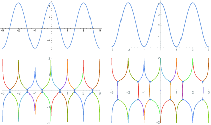
Figure 15: Left: Plot of $m_{D}(t)$ and the Stokes lines. One can see that the MTP appears at each massless point (when the states cross in the light of the Landau-Zener model). Right: $m_{D}$ cannot be massless because of large $m_{0}$. Since the local linear approximation is not valid at the minimum of $m_{D}$, the corresponding scattering problem is not for the quadratic potential, but for the (higher) quartic potential. One can see that the Stokes lines are giving the structure of the quartic scatteringEnomoto:2020xlf at each minimum.

We thus confirmed that the linear expansion at the crossing point, which is used in the Landau-Zener model, is justified because of the separable structure of the Stokes lines.

On the other hand, if one chooses $m(t)=m_{0}+A\cos(at/\hbar)$, in which $\hbar$ is explicit, one will find an additional imaginary part in

$$Q_{0} = -k^{2}-\left(m_{0}+A\cos\frac{at}{\hbar}\right)^{2}-iaA\sin\frac{at}{\hbar},$$

which unmerges the MTP. The Stokes lines are shown in Fig.16, which have the expected structure.

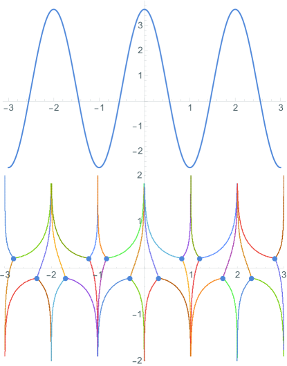
Figure 16: A plot of $m(t)$ and the Stokes lines when $\hbar^{-1}$ is explicit in the phase of the periodic function. One can see that the MTP is unmerged by the imaginary part.

On the other hand, if one expands this (latter) $m_{D}$ at the massless point ($t=t_{i}$), one will have

$$m_{D} \simeq m_{0}+\frac{1}{\hbar}\left[Aa\sin\frac{at_{i}}{\hbar}\right](t-t_{i}),$$ (273)

which formally ruins the WKB expansion since it contains an extra $\hbar{{}^{-1}}$ in the “small” part. In this sense, it would be better to define $\omega\equiv a/\hbar$ to control the $\hbar$ expansion before discussing the local (linear) expansion.

Finally, let us see what happens if $m_{D}(t)$ has a bump;

$$m_{D}(t) = m_{0}\pm\frac{Ae^{\gamma t}}{\left(1+e^{\gamma t}\right)^{2}}.$$ (274)

In this case, the massless points can appear only for the minus sign. We show the Stokes lines in Fig.17, which shows the expected MTP-like structure on the left. On the right, however, the Stokes phenomena seem to be possible although state crossing (in the light of the Landau-Zener model) does not appear. The particle production without state crossing can be verified by numerical calculation, although the magnitude is suppressed.

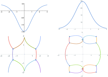
Figure 17: Left: Plot of $m_{D}(t)$ and the Stokes lines when $m_{D}$ has $m_{D}=0$ for real $t$. One can see that the MTP-like structure appears at each massless point. (The Stokes lines are infinitely degenerated in this case.) Right: Although $m_{D}$ cannot have $m_{D}=0$ for real $t$, the Stokes lines are crossing the real $t$ axis. This suggests that particle production may take place when the velocity increases.

Also in this case, the introduction of $\hbar$ in the exponents causes a split of the MTP-like structure. For example, one can consider

$$m_{D}(t) = m_{0}\pm\frac{Ae^{\frac{at}{\hbar}}}{\left(1+e^{\frac{at}{\hbar}}\right)^{2}},$$ (275)

which introduces the additional imaginary part in $Q_{0}$. The Stokes lines are shown in Fig.18.

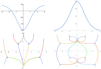
Figure 18: Left: Plot of $m_{D}(t)$ and the Stokes lines when $m_{D}$ can cross $m_{D}=0$. Right: When $m_{D}$ cannot cross $m_{D}=0$. The Stokes lines split due to the imaginary part.

Appendix C Distribution of Majorana fermion

In this section, we show the formula of the distribution function of the Majorana fermion described by the wave functions and its equation of evolution.

C.1 Distribution formula

Using the mode expansion (60), the Hamiltonian can be represented as

$$H = \int d^{3}x\left(-\psi_{R}^{\dagger}i\bar{\sigma}^{i}\partial_{i}\psi_{R}+\frac{1}{2}m_{R}\psi_{R}^{2}+\frac{1}{2}m_{R}^{*}\psi_{R}^{\dagger 2}\right)$$ (276)

$$= \int\frac{d^{3}k}{(2\pi)^{3}}\sum_{s=\pm}\frac{1}{2}\left[E_{k}^{s}(a_{\bm{k}}^{s\dagger}a_{\bm{k}}^{s}-a_{-\bm{k}}^{s}a_{-\bm{k}}^{s\dagger})\right.$$

$$\left.\qquad\qquad\qquad+\left(F_{k}^{s}\cdot e^{i\theta_{\bm{k}}}a_{-\bm{k}}^{s}a_{\bm{k}}^{s}+({\rm h.c.})\right)\right]$$

$$= \int\frac{d^{3}k}{(2\pi)^{3}}\sum_{s=\pm}\frac{1}{2}(\begin{array}[]{cc}a_{\bm{k}}^{s\dagger}&e^{i\theta_{\bm{k}}}a_{-\bm{k}}^{s}\end{array})$$ (283)

$$\qquad\qquad\quad\times\left(\begin{array}[]{cc}E_{k}^{s}&F_{k}^{s*}\\ F_{k}^{s}&-E_{k}^{s}\end{array}\right)\left(\begin{array}[]{c}a_{\bm{k}}^{s}\\ e^{-i\theta_{\bm{k}}}a_{-\bm{k}}^{s\dagger}\end{array}\right)$$

where

$$E_{k}^{s} \equiv -s|{\bm{k}}|(|u_{k}^{s}|^{2}-|v_{k}^{s}|^{2})+sm_{R}u_{k}^{s}v_{k}^{s*}+sm_{R}^{*}u_{k}^{s*}v_{k}^{s},$$

$$F_{k}^{s} \equiv -2s|{\bm{k}}|u_{k}^{s}v_{k}^{s}-sm_{R}(u_{k}^{s})^{2}+sm_{R}^{*}(v_{k}^{s})^{2}.$$ (285)

Note that $E_{k}^{s}$ and $F_{k}^{s}$ have a nontrivial relation

$$(E_{k}^{s})^{2}+|F_{k}^{s}|^{2}=\omega_{k}^{2},\qquad\omega_{k}\equiv\sqrt{|{\bm{k}}|^{2}+|m_{R}|^{2}}$$ (286)

because of the normalization of the wave functions $|u_{k}^{s}|^{2}+|v_{k}^{s}|^{2}=1.$ To obtain the number operator, we diagonalize the Hamiltonian (283) using the (time-dependent) Bogoliubov transformation

$$a_{\bm{k}}^{s}=\alpha_{k}^{s}(t)\bar{a}_{\bm{k}}^{s}(t)+\beta_{k}^{s}(t)\cdot e^{-i\theta_{\bm{k}}}\bar{a}_{-\bm{k}}^{s\dagger}(t),$$ (287)

where $\alpha_{k}^{s}$ and $\beta_{k}^{s}$ are the Bogoliubov “coefficients” that satisfy

$$|\alpha_{k}^{s}|^{2}+|\beta_{k}^{s}|^{2}=1.$$ (288)

Substituting (287) into (283), the Hamiltonian can be represented in terms of $\bar{a}_{\bm{k}}^{s}$-basis as

$$H = \int\frac{d^{3}k}{(2\pi)^{3}}\sum_{s=\pm}\frac{1}{2}(\begin{array}[]{cc}\bar{a}_{\bm{k}}^{s\dagger}&e^{i\theta_{\bm{k}}}\bar{a}_{-\bm{k}}^{s}\end{array})$$ (295)

$$\qquad\qquad\quad\times\left(\begin{array}[]{cc}\bar{E}_{k}^{s}&\bar{F}_{k}^{s*}\\ \bar{F}_{k}^{s}&-\bar{E}_{k}^{s}\end{array}\right)\left(\begin{array}[]{c}\bar{a}_{\bm{k}}^{s}\\ e^{-i\theta_{\bm{k}}}\bar{a}_{-\bm{k}}^{s\dagger}\end{array}\right)$$

where

$$\bar{E}_{k}^{s} = (|\alpha_{k}^{s}|^{2}-|\beta_{k}^{s}|^{2})E_{k}^{s}-\alpha_{k}^{s}\beta_{k}^{s}F_{k}^{s}-\alpha_{k}^{s*}\beta_{k}^{s*}F_{k}^{s*}$$ (296)

$$\bar{F}_{k}^{s} = 2\alpha_{k}^{s}\beta_{k}^{s*}E_{k}^{s}+(\alpha_{k}^{s})^{2}F_{k}^{s}-(\beta_{k}^{s*})^{2}F_{k}^{s*}.$$ (297)

As $\bar{F}_{k}^{s}=0$ is chosen to diagonalize Hamiltonian, one can obtain

$$|\beta_{k}^{s}|^{2}=\frac{1}{2}\left(1-\frac{E_{k}^{s}}{\omega_{k}}\right),\qquad\alpha_{k}^{s}=-\frac{\omega_{k}+E_{k}^{s}}{F_{k}^{s}}\beta_{k}^{s*}.$$ (298)

Hence the Hamiltonian can be diagonalized as

$$H = \int\frac{d^{3}k}{(2\pi)^{3}}\sum_{s=\pm}\frac{1}{2}(\begin{array}[]{cc}\bar{a}_{\bm{k}}^{s\dagger}&e^{i\theta_{\bm{k}}}\bar{a}_{-\bm{k}}^{s}\end{array})$$ (305)

$$\qquad\qquad\times\left(\begin{array}[]{cc}\omega_{k}&\\ &-\omega_{k}\end{array}\right)\left(\begin{array}[]{c}\bar{a}_{\bm{k}}^{s}\\ e^{-i\theta_{\bm{k}}}\bar{a}_{-\bm{k}}^{s\dagger}\end{array}\right)$$

$$= \int\frac{d^{3}k}{(2\pi)^{3}}\sum_{s=\pm}\omega_{k}\left(\bar{a}_{\bm{k}}^{s\dagger}\bar{a}_{\bm{k}}^{s}-\frac{1}{2}\int d^{3}x\right).$$ (306)

The distribution function $n_{k}^{s}$ can be obtained by the time-dependent occupation operator and the initial vacuum state defined by $a_{\bm{k}}^{s}|0\rangle=0$ as

$$n_{k}^{s}(t) = \frac{\langle 0|\bar{a}_{\bm{k}}^{s\dagger}\bar{a}_{\bm{k}}^{s}|0\rangle}{\int d^{3}x}$$ (307)

$$= |\beta_{k}^{s}|^{2}\>=\>\frac{1}{2}\left(1-\frac{E_{k}^{s}}{\omega_{k}}\right).$$ (308)

C.2 Zero particle state

Before we derive the evolution equation of the distribution function, we discuss the specific representation of each wave function in the zero particle state. The zero particle state $n_{k}^{s}=0$ corresponds to $E_{k}^{s}=\omega_{k}$ and $F_{k}^{s}=0$, that are equivalent to

$$\omega_{k} = -s|{\bm{k}}|(|u_{k}^{s}|^{2}-|v_{k}^{s}|^{2})+sm_{R}u_{k}^{s}v_{k}^{s*}+sm_{R}^{*}u_{k}^{s*}v_{k}^{s},$$

$$0 = -2s|{\bm{k}}|u_{k}^{s}v_{k}^{s}-sm_{R}(u_{k}^{s})^{2}+sm_{R}^{*}(v_{k}^{s*})^{2}$$ (310)

from (LABEL:eq:def_E) and (285). Solving the above equations about the wave functions $u_{k}^{s}$ and $v_{k}^{s}$, one can obtain

$$u_{k}^{s} = e^{i\alpha}\cdot\sqrt{\frac{1}{2}\left(1-\frac{sk}{\omega_{k}}\right)},$$ (311)

$$v_{k}^{s} = e^{i\alpha}\cdot\frac{sm_{R}}{|m_{R}|}\sqrt{\frac{1}{2}\left(1+\frac{sk}{\omega_{k}}\right)}$$ (312)

where $\alpha$ is an arbitrary phase. Note that the above results mean not functional solutions but just values at a time to be $n_{k}^{s}=0$.

C.3 Equation of evolution

In this section, we consider obtaining the equation of evolution of the distribution function (308). Note that the original equations of motion of the wave functions (II.1) seem $2\times 2=4$ real degrees, but the actual degrees are $4-1=3$ because there is a conservation law

$$|u_{k}^{s}(t)|^{2}+|v_{k}^{s}(t)|^{2}=1.$$ (313)

Since the distribution $n_{k}^{s}$ is described by $E_{k}^{s}$ that includes $|u_{k}^{s}|^{2}-|v_{k}^{s}|^{2}$ (1 real degree) and $u_{k}^{s}v_{k}^{s*}$ (2 real degrees), it is enough to follow the evolution of these functions. The time derivatives of these functions are given by

$$\partial_{t}(|u_{k}^{s}|^{2}-|v_{k}^{s}|) = 2is(m_{R}u_{k}^{s}v_{k}^{s*}-m_{R}^{*}u_{k}^{s*}v_{k}^{s}),$$ (314)

$$\partial_{t}[u_{k}^{s}v_{k}^{s*}] = ism_{R}^{*}(|u_{k}^{s}|^{2}-|v_{k}^{s}|^{2})+2isku_{k}^{s}v_{k}^{s*},$$

that can be represented by a matrix form as

$$\partial_{t}\left(\begin{array}[]{c}|u_{k}^{s}|^{2}-|v_{k}^{s}|\\ u_{k}^{s}v_{k}^{s*}\\ u_{k}^{s*}v_{k}^{s}\end{array}\right)=isF\left(\begin{array}[]{c}|u_{k}^{s}|^{2}-|v_{k}^{s}|\\ u_{k}^{s}v_{k}^{s*}\\ u_{k}^{s*}v_{k}^{s}\end{array}\right)$$ (316)

$$F\equiv\left(\begin{array}[]{ccc}0&2m_{R}&-2m_{R}^{*}\\ m_{R}^{*}&2k&0\\ -m_{R}&0&-2k\end{array}\right).$$ (317)

Eq.(316) indicates the equations are closed within the three functions. Because $E_{k}^{s}$ is described by the three functions $|u_{k}^{s}|^{2}-|v_{k}^{s}|^{2},$ $u_{k}^{s}b_{k}^{s*}$, $u_{k}^{s*}b_{k}^{s}$, the arbitrary higher derivations of $E_{k}^{s}$ also be described by those three functions. This fact indicates that $E_{k}^{s}$, $\dot{E}_{k}^{s}$, $\ddot{E}_{k}^{s}$ can be independent, and thus the higher derivatives $\partial_{t}^{n}E_{k}^{s}$ ($n\geq 3$) can be described by a linear combination of $E_{k}^{s}$, $\dot{E}_{k}^{s}$, $\ddot{E}_{k}^{s}$. Since the time derivatives of $E_{k}^{s}$ in (LABEL:eq:def_E) are given by

$$\dot{E}_{k}^{s} = s\dot{m}_{R}\cdot u_{k}^{s}v_{k}^{s*}+s\dot{m}_{R}\cdot u_{k}^{s*}v_{k}^{s},$$ (318)

$$\ddot{E}_{k}^{s} = i(m_{R}^{*}\dot{m}_{R}-\dot{m}_{R}^{*}m_{R})(|u_{k}^{s}|^{2}-|v_{k}^{s}|^{2})$$

$$+(s\ddot{m}_{R}+2ik\dot{m}_{R})u_{k}^{s}v_{k}^{s*}+(s\ddot{m}^{*}_{R}*-2ik\dot{m}_{R}^{*})u_{k}^{s*}v_{k}^{s},$$

one can obtain the matrix representation as

$$\left(\begin{array}[]{c}E_{k}^{s}\\ \dot{E}_{k}^{s}\\ \ddot{E}_{k}^{s}\end{array}\right)=sG\left(\begin{array}[]{c}|u_{k}^{s}|^{2}-|v_{k}^{s}|^{2}\\ u_{k}^{s}v_{k}^{s*}\\ u_{k}^{s*}v_{k}^{s}\end{array}\right)$$ (320)

$$G \equiv \left(\begin{array}[]{ccc}-k&m_{R}&m_{R}^{*}\\ 0&\dot{m}_{R}&\dot{m}_{R}^{*}\\ is(m_{R}^{*}\dot{m}_{R}-\dot{m}_{R}^{*}m_{R})&\ddot{m}_{R}+2isk\dot{m}_{R}&\ddot{m}_{R}^{*}-2isk\dot{m}_{R}^{*}\end{array}\right).$$ (324)

Hence, the evolution of a set of $E_{k}^{s}$s are described by

$$\partial_{t}\left(\begin{array}[]{c}E_{k}^{s}\\ \dot{E}_{k}^{s}\\ \ddot{E}_{k}^{s}\end{array}\right) = s\dot{G}\left(\begin{array}[]{c}|u_{k}^{s}|^{2}-|v_{k}^{s}|^{2}\\ u_{k}^{s}v_{k}^{s*}\\ u_{k}^{s*}v_{k}^{s}\end{array}\right)+iGF\left(\begin{array}[]{c}|u_{k}^{s}|^{2}-|v_{k}^{s}|^{2}\\ u_{k}^{s}v_{k}^{s*}\\ u_{k}^{s*}v_{k}^{s}\end{array}\right)$$ (335)

$$= \left(\dot{G}+isGF\right)G^{-1}\left(\begin{array}[]{c}E_{k}^{s}\\ \dot{E}_{k}^{s}\\ \ddot{E}_{k}^{s}\end{array}\right).$$ (340)

In general, the components of $\left(\dot{G}+isGF\right)G^{-1}$ are given by

$$\left(\dot{G}+isGF\right)G^{-1}=\left(\begin{array}[]{ccc}0&1&0\\ 0&0&1\\ f_{1}&f_{2}&f_{3}\end{array}\right)$$ (341)

where $f_{1},f_{2},f_{3}$ are functions that consist of the time-dependent mass $m_{R}$, helicity $s$, and the momentum $|\bm{k}|$.

Let us consider a special case $\ddot{m}_{R}=0$. Then one can obtain simple results:

$$f_{1}=4{\rm Re}[m_{R}^{*}\dot{m}_{R}],\quad f_{2}=-4\omega_{k}^{2},\quad f_{3}=0,$$ (342)

that lead

$$\dddot{E}_{k}^{s} = f_{1}E_{k}^{s}+f_{2}\dot{E}_{k}^{s}+f_{2}\ddot{E}_{k}^{s}$$ (343)

$$= 4{\rm Re}[m_{R}^{*}\dot{m}_{R}]\cdot E_{k}^{s}-4\omega_{k}^{2}\dot{E}_{k}^{s}.$$

Choosing the initial condition to be the zero particle state, each of the initial values is given by

$$\left(\begin{array}[]{c}E_{k}^{s}\\ \dot{E}_{k}^{s}\\ \ddot{E}_{k}^{s}\end{array}\right)=\left(\begin{array}[]{c}\omega_{k}\\ {\rm Re}[m_{R}^{*}\dot{m}_{R}]/\omega_{k}\\ 0\end{array}\right)$$ (344)

where we used (311), (312), and (320). Note in this case that $E_{k}^{s}$ can evolve but $E_{k}^{+}-E_{k}^{-}$ cannot because the equation of evolution is described by

$$\partial_{t}^{3}(E_{k}^{+}-E_{k}^{-}) = 4{\rm Re}[m_{R}^{*}\dot{m}_{R}]\cdot(E_{k}^{+}-E_{k}^{-})$$ (345)

$$-4\omega_{k}^{2}\cdot\partial_{t}(E_{k}^{+}-E_{k}^{-})$$

and all the initial values of $E_{k}^{+}-E_{k}^{-}$, $\partial_{t}(E_{k}^{+}-E_{k}^{-})$, $\partial_{t}^{2}(E_{k}^{+}-E_{k}^{-})$ are zero. Thus, we can conclude that the net number

$$n_{k}^{+}-n_{k}^{-}=-\frac{E_{k}^{+}-E_{k}^{-}}{2\omega_{k}}$$ (346)

also never develops from the zero particle state in the case of $\ddot{m}_{R}=0$. One can also obtain the same statement in the case of $\bm{k}=0$.

References

- (1) A. G. Cohen, D. B. Kaplan and A. E. Nelson, “Spontaneous baryogenesis at the weak phase transition,” Phys. Lett. B 263 (1991), 86-92
- (2) A. G. Cohen and D. B. Kaplan, “Thermodynamic Generation of the Baryon Asymmetry,” Phys. Lett. B 199 (1987) 251.
- (3) A. G. Cohen and D. B. Kaplan, “Spontaneous Baryogenesis,” Nucl. Phys. B 308 (1988) 913.
- (4) A. D. Sakharov, “Violation of CP Invariance, C asymmetry, and baryon asymmetry of the universe,” Sov. Phys. Usp. 34 (1991) no.5, 392-393
- (5) E. V. Arbuzova, A. D. Dolgov and V. A. Novikov, “General properties and kinetics of spontaneous baryogenesis,” Phys. Rev. D 94 (2016) no.12, 123501; E. V. Arbuzova and A. D. Dolgov, “Problems of spontaneous and gravitational baryogenesis,” 1712.04627.
- (6) L. Pearce, L. Yang, A. Kusenko and M. Peloso, “Leptogenesis via neutrino production during Higgs condensate relaxation,” Phys. Rev. D 92 (2015) no.2, 023509 [arXiv:1505.02461 [hep-ph]].
- (7) P. Adshead and E. I. Sfakianakis, “Leptogenesis from left-handed neutrino production during axion inflation,” Phys. Rev. Lett. 116 (2016) no.9, 091301 [arXiv:1508.00881 [hep-ph]].
- (8) P. Adshead and E. I. Sfakianakis, “Fermion production during and after axion inflation,” JCAP 1511 (2015) 021
- (9) A. Kusenko, L. Pearce and L. Yang, “Postinflationary Higgs relaxation and the origin of matter-antimatter asymmetry,” Phys. Rev. Lett. 114 (2015) no.6, 061302 [arXiv:1410.0722 [hep-ph]].
- (10) L. Yang, L. Pearce and A. Kusenko, “Leptogenesis via Higgs Condensate Relaxation,” Phys. Rev. D 92 (2015) no.4, 043506 [arXiv:1505.07912 [hep-ph]].
- (11) Y. P. Wu, L. Yang and A. Kusenko, “Leptogenesis from spontaneous symmetry breaking during inflation,” JHEP 12 (2019), 088 [arXiv:1905.10537 [hep-ph]].
- (12) Y. B. Zeldovich and A. A. Starobinsky, Particle production and vacuum polarization in an anisotropic gravitational field, Sov. Phys. JETP 34 (1972) 1159.
- (13) A. Dolgov and K. Freese, “Calculation of particle production by Nambu Goldstone bosons with application to inflation reheating and baryogenesis,” Phys. Rev. D 51 (1995), 2693-2702 [arXiv:hep-ph/9410346 [hep-ph]].
- (14) A. Dolgov, K. Freese, R. Rangarajan and M. Srednicki, “Baryogenesis during reheating in natural inflation and comments on spontaneous baryogenesis,” Phys. Rev. D 56 (1997) 6155
- (15) K. Funakubo, A. Kakuto, S. Otsuki and F. Toyoda, “Charge generation in the oscillating background,” Prog. Theor. Phys. 105 (2001), 773-788 [arXiv:hep-ph/0010266 [hep-ph]].
- (16) R. Rangarajan and D. V. Nanopoulos, “Inflationary baryogenesis,” Phys. Rev. D 64 (2001), 063511 [arXiv:hep-ph/0103348 [hep-ph]].
- (17) A. Kusenko, K. Schmitz and T. T. Yanagida, “Leptogenesis via Axion Oscillations after Inflation,” Phys. Rev. Lett. 115 (2015) no.1, 011302 [arXiv:1412.2043 [hep-ph]].
- (18) S. Enomoto and T. Matsuda, “Asymmetric preheating,” Int. J. Mod. Phys. A 33 (2018) no.25, 1850146 [arXiv:1707.05310 [hep-ph]].
- (19) S. Enomoto and T. Matsuda, “Baryogenesis from the Berry phase,” Phys. Rev. D 99 (2019) no.3, 036005 [arXiv:1811.06197 [hep-th]].
- (20) S. Enomoto, C. Cai, Z. H. Yu and H. H. Zhang, “Leptogenesis due to oscillating Higgs field,” Eur. Phys. J. C 80 (2020) no.12, 1098 [arXiv:2005.08037 [hep-ph]].
- (21) A. D. Dolgov and D. P. Kirilova, “On Particle Creation By A Time Dependent Scalar Field,” Sov. J. Nucl. Phys. 51, 172 (1990) [Yad. Fiz. 51, 273 (1990)].
- (22) L. Kofman, A. D. Linde and A. A. Starobinsky, “Towards the theory of reheating after inflation,” Phys. Rev. D 56 (1997) 3258 [hep-ph/9704452].
- (23) J. S. Schwinger, “On gauge invariance and vacuum polarization,” Phys. Rev. 82 (1951), 664-679
- (24) S. Shakeri, M. A. Gorji and H. Firouzjahi, “Schwinger Mechanism During Inflation,” Phys. Rev. D 99 (2019) no.10, 103525
- (25) H. Kitamoto, “No-go theorem of anisotropic inflation via Schwinger mechanism,” Phys. Rev. D 103 (2021), 063521 [arXiv:2010.10388 [hep-th]].
- (26) H. Taya, T. Fujimori, T. Misumi, M. Nitta and N. Sakai, “Exact WKB analysis of the vacuum pair production by time-dependent electric fields,” JHEP 03 (2021), 082 [arXiv:2010.16080 [hep-th]].
- (27) T. Matsuda, “On the cosmological domain wall problem in supersymmetric models,” Phys. Lett. B 436 (1998), 264-268 [arXiv:hep-ph/9804409 [hep-ph]].
- (28) A. D. Dolgov, S. I. Godunov, A. S. Rudenko and I. I. Tkachev, “Separated matter and antimatter domains with vanishing domain walls,” JCAP 10 (2015), 027 [arXiv:1506.08671 [astro-ph.CO]].
- (29) A. E. Nelson, D. B. Kaplan and A. G. Cohen, “Why there is something rather than nothing: Matter from weak interactions,” Nucl. Phys. B 373 (1992), 453-478
- (30) K. Funakubo, A. Kakuto, S. Otsuki and F. Toyoda, “Numerical approach to CP violating Dirac equation,” Prog. Theor. Phys. 95 (1996), 929-942 [arXiv:hep-ph/9602269 [hep-ph]].
- (31) S. Enomoto and T. Matsuda, “The exact WKB for cosmological particle production,” JHEP 03 (2021), 090 [arXiv:2010.14835 [hep-ph]].
- (32) N. Sueishi, S. Kamata, T. Misumi and M. Ünsal, JHEP 12 (2020), 114 doi:10.1007/JHEP12(2020)114 [arXiv:2008.00379 [hep-th]].
- (33) N. Sueishi, S. Kamata, T. Misumi and M. Ünsal, “Exact-WKB, complete resurgent structure, and mixed anomaly in quantum mechanics on ,” [arXiv:2103.06586 [quant-ph]].
- (34) T. Kawai, Y. Takei and G. Kato, “Algebraic Analysis of Singular Perturbation Theory” ISBN 978-0821835470; N. Honda, T. Kawai and Y. Takei, “Virtual Turning Points”, Springer (2015), ISBN 978-4431557029.
- (35) C. Zener, “Nonadiabatic crossing of energy levels,” Proc. Roy. Soc. Lond. A 137 (1932) 696.
- (36) T. Aoki, H. Majima, Y. Takei, N. Tose (Eds.) “Algebraic analysis of differential equations: From microlocal analysis to exponential asymptotics festschrift in honor of Takahiro Kawai” ISBN 9784431732396; E. Delabaere and F. Pham, “Resurgent methods in semi-classical asymptotics, Ann. Inst. H. Poincare, 71(1999),1-94.
- (37) P. B. Greene and L. Kofman, “Preheating of fermions,” Phys. Lett. B 448 (1999) 6
- (38) M. Peloso and L. Sorbo, “Preheating of massive fermions after inflation: Analytical results,” JHEP 0005 (2000) 016
- (39) L. Kofman, A. D. Linde, X. Liu, A. Maloney, L. McAllister and E. Silverstein, “Beauty is attractive: Moduli trapping at enhanced symmetry points,” JHEP 05 (2004), 030 [arXiv:hep-th/0403001 [hep-th]].
- (40) S. Enomoto, S. Iida, N. Maekawa and T. Matsuda, “Beauty is more attractive: particle production and moduli trapping with higher dimensional interaction,” JHEP 01 (2014), 141 [arXiv:1310.4751 [hep-ph]].
- (41) I. Affleck and M. Dine, “A New Mechanism for Baryogenesis,” Nucl. Phys. B 249 (1985), 361-380
- (42) T. Matsuda, “Affleck-Dine baryogenesis after thermal brane inflation,” Phys. Rev. D 65 (2002), 103501 [arXiv:hep-ph/0202209 [hep-ph]].
- (43) T. D. Lee and Y. Pang, “Nontopological solitons,” Phys. Rept. 221 (1992), 251-350
- (44) T. Matsuda, “Affleck-Dine baryogenesis in the local domain,” Phys. Rev. D 65 (2002), 103502 [arXiv:hep-ph/0202211 [hep-ph]].
- (45) M. V. Berry and K. Mount, “Semiclassical approximations in wave mechanics,” Rept. Prog. Phys. 35 (1972), 315
- (46) H. Shen and H. J. Silverstone: Observations on the JWKB treatment of the quadratic barrier, Algebraic analysis of differential equations from microlocal analysis to exponential asymptotics, Springer, 2008, pp. 237 - 250.
- (47) T. Aoki, T. Kawai, and T. Takei: The Bender-Wu analysis and the Voros theory, II, Adv. Stud. Pure Math. 54 (2009), Math. Soc. Japan, Tokyo, 2009, pp. 19 -94
-
(48)
A simple Stokes-line drawer for Mathematica can be downloaded from
https://www.sit.ac.jp/user/matsuda/img/EWKB.zip