Learning Residue-Aware Correlation Filters and Refining Scale Estimates with the GrabCut for Real-Time UAV Tracking

Abstract

Unmanned aerial vehicle (UAV)-based tracking is attracting increasing attention and developing rapidly in applications such as agriculture, aviation, navigation, transportation and public security. Recently, discriminative correlation filters (DCF)-based trackers have stood out in UAV tracking community for their high efficiency and appealing robustness on a single CPU. However, due to limited onboard computation resources and other challenges the efficiency and accuracy of existing DCF-based approaches is still not satisfying. In this paper, we explore using segmentation by the GrabCut to improve the wildly adopted discriminative scale estimation in DCF-based trackers, which, as a mater of fact, greatly impacts the precision and accuracy of the trackers since accumulated scale error degrades the appearance model as online updating goes on. Meanwhile, inspired by residue representation, we exploit the residue nature inherent to videos and propose residue-aware correlation filters that show better convergence properties in filter learning. Extensive experiments are conducted on four UAV benchmarks, namely, UAV123@10fps, DTB70, UAVDT and Vistrone2018 (VisDrone2018-test-dev). The results show that our method achieves state-of-the-art performance.

1 Introduction

Unmanned aerial vehicle (UAV)-based tracking is an emerging task and has attracted increasing attention in recent years. It has various applications, e.g., aerial patrolling[30], disaster response [74], autonomously landing [43], wildlife protection [54]. Compared with general tracking scenes, UAV tracking faces more onerous challenges, e.g., motion blur, severe occlusion, extreme visual angle and scale change, and scarce computation resources [22].

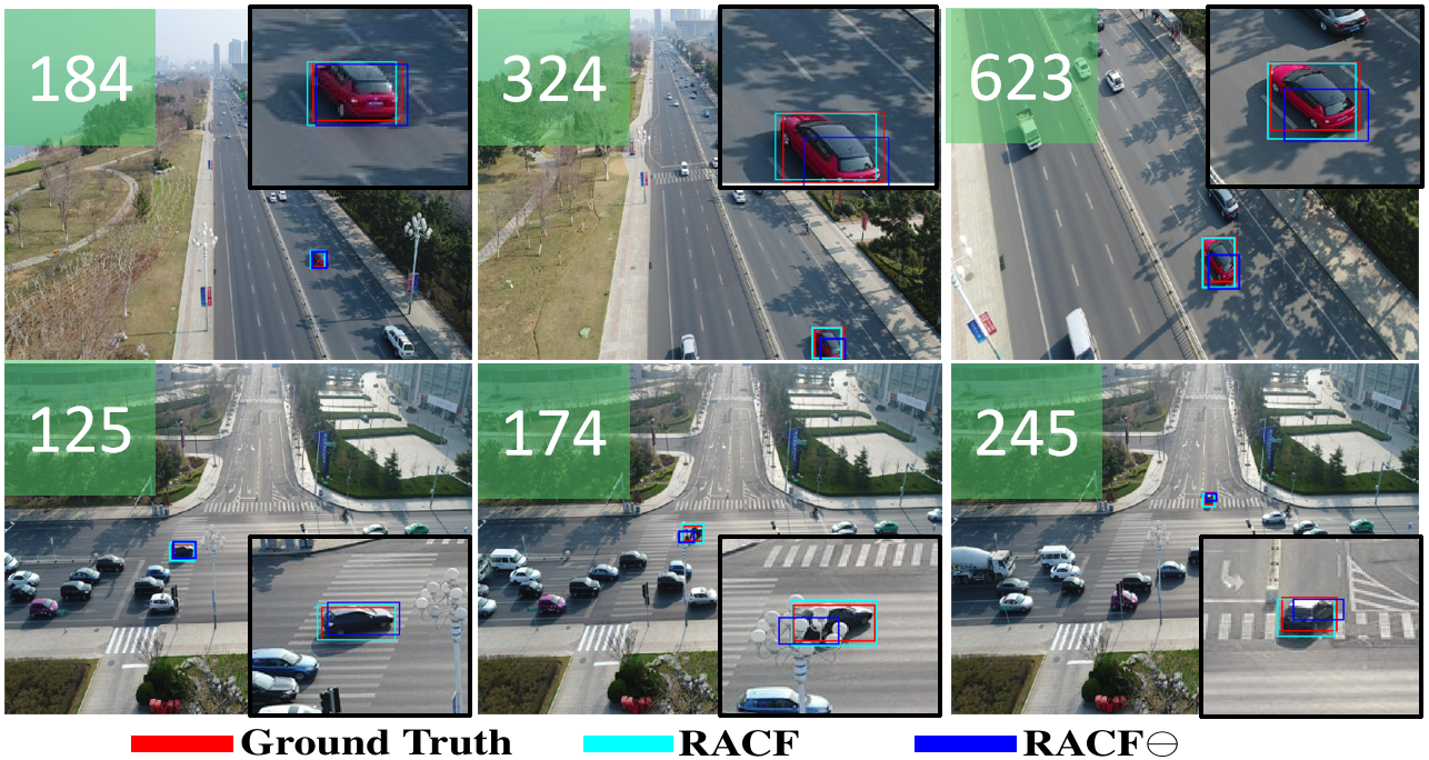
Figure 1: Comparison of our trackers RACF and RACF$\ominus$. RACF uses the GrabCut to refine the scale estimates whereas RACF$\ominus$ uses the existing discriminative scale estimation only.

Despite deep learning-based approaches have achieved great success and are promising in dealing with these challenges [14, 44, 65, 4, 34, 70], its efficiency is unsatisfactory in the limitation of power capacity and computational resources onboard UAVs. In contrast, discriminative correlation filters (DCF)-based methods are more favorable in efficiency for UAV tracking thanks to the fast Fourier transform (FFT) [29, 38, 23, 40, 32, 42, 39, 27] but they are not comparable with deep learning-based method in terms of precision and accuracy. One important reason is the failing to recognize the problems with the discriminative scale estimation [41, 18] used in DCF-based trackers. First, applying the filter at limited predefined multiple resolutions is inaccurate in estimating continuous changes of scale. Second, a fixed aspect ratio of target size is usually adopted to balance accuracy and speed in scale estimation, which is very rough and degrades the tracking greatly in situations where targets undergo extreme visual angle and appearance variations. See Fig. 1 for examples. As can be seen, the RACF$\ominus$ tracker using the existing discriminative scale estimation performs badly when the two target cars undergo big visual angle changes. Therefore, the existing discriminative scale estimation is inaccurate, which in fact greatly impacts the precision and accuracy of the trackers, since accumulated scale error degrades the appearance model as online updating goes on. In this paper, we study using the segmentation algorithm GrabCut [57] to improve scale estimation of DCF-based trackers. The method is demonstrated by the tracker RACF shown in Fig. 1 .

On the other hand, most DCF-based methods improve precision and accuracy at the cost of efficiency. For instance, the aberrance repressed correlation filters (ARCF) [29] has achieved state-of-the-art performance in UAV tracking by repressing aberrances happening during the tracking process, but it takes five iterations of ADMM (Alternating Direction Method of Multipliers) at each frame for model update, which is time-consuming compared with two iterations in its baseline the background-aware correlation filters (BACF) [24]. Inspired by the fast and stable optimization of Residual Networks (ResNets) [26], we exploit the residue nature inherent to videos and propose residue-aware correlation filters (RACF) that show better convergence properties in filter learning, which, to the best of our knowledge, has not been studied in DCF-based trackers before. In addition, ARCF does not use spatial and temporal regularizations which have been proved effective for suppressing boundary effects and avoiding overfitting to inaccurate and noisy samples [15, 33, 36, 38]. In this paper, we succeed to add spatial and temporal regularizations to boot performance with little additional computational cost. The contributions of this paper are summarized as follows:

• We propose a novel scale estimation approach for DCF-based trackers by using the GrabCut [57] algorithm to refine the discriminative scale estimates, which can be incorporated easily into any tracking method with discriminative scale estimation to improve precision and accuracy.

• We propose a novel regularization to model the residue between two neighboring frames, resulting in what we call residue-aware correlation filters, which show better convergence properties in filter learning. Meanwhile, we add spatial and temporal regularizations to boot performance with little additional computational cost.

• We demonstrate the proposed methods on four UAV benchmarks, namely, UAV123@10fps [50], DTB70 [35], UAVDT [20] and Vistrone2018 (VisDrone2018-test-dev) [72]. Experimental results show that the proposed approaches achieves state-of-the-art performance.

2 Related Works

2.1 Discriminative correlation filters

Using DCF for visual tracking starts with the minimum output sum of squared error (MOSSE) filter [6]. Afterwards, kernel trick [28], discriminative scale estimation [41, 18], spatial and temporal regularizations [15, 33], deep features [46, 17], attention [27], context and background information [51, 24] and so on were introduced for improvement. Among these DCF-based trackers, we are interested in the background-aware correlation filters (BACF) [24]. For one thing, it expands search region with lower computational cost and also has some theoretical advantages as shown in [36], an equivalent approach but formulated and optimized differently. For another, BACF equipped with an aberrance regularization and an enhanced feature extractor, i.e., the aberrance repressed correlation filters (ARCF) [29], has achieved state-of-the-art performance in multiple benchmarks specified for UAV tracking. These two methods are in close connection with our work here.

2.2 Residual representations

In visual tracking, residual learning was applied to capture the difference between the base layer output and the ground truth to reduce model degradation during online update in [59]. Before that residual representations had found their usefulness in image retrieval, recognition and restoration [26, 64, 10], video compression [62] and equation solving [53]. It has been shown [61, 9] that the solvers aware of the residual nature of the solutions converge much faster than standard solvers [61, 53, 26]. To understand the optimization landscape of the well-known ResNets [26], it has been proved that residual networks eliminate singularities and reduce shattered gradient, leading to numerical stability and easier optimization [55, 3, 31]. In the literature, residuals can be the difference between the target and the model output, the difference between the input and the output, the difference between a sample and the sample mean. In this paper, a residue is formed by subtracting the feature of the current frame from that of the previous one and the residue representation of the current frame is the sum of the residue and the feature of the previous frame. Since, approximately, videos are temporally continuous, the residues are usually of small values and entropy, which can be used to speed up the learning of correlation filters.

2.3 Scale estimation

There are three typical discriminative scale estimation strategies in DCF-based visual tracking [48, 71]. i) Multi-resolution translation filter (MRTF) defines a scale pool and estimates target scale by applying the translation filter on images of different scales [41, 5]. ii) Joint scale-space filter (JSSF) jointly estimates the translation and scale of the target by simultaneously maximizing the scores of translation and scale filters with a three-dimensional Gaussian function as the desired response. iii) Separate scale filter (SSF) learns a separate 1-dimensional scale correlation filter for scale estimation independent of translation [19, 18]. The SSF strategy has been popular in DCF-based trackers for its effectiveness, efficiency, robustness and easy integration. Although there are some variants such as using subgrid interpolation for efficiency [18], combining a points tracker for abrupt scale changes [1], defining rotation-aware correlation filters [47] and utilizing deep features for scale filter [48], these methods for scale estimation essentially remain detection-based and therefore inaccurate.

Recently, many researchers have noticed the close relation between video object segmentation and visual tracking and combined them to improve respective performance [70, 44, 11, 60]. It makes sense since accurate segmentation results provide reliable object observations for tracking and in turn precise target states provided by a reliable tracker correctly guide and speed up object segmentation. Unfortunately, they are deep learning-based approaches, not suitable for UAV tracking with limited onboard resources. There do exist plenty of CPU-based methods earlier by combing tracking and segmentation to overcome the inaccurate object description with rectangular bounding box, especially for tracking non-rigid objects [2, 56, 21, 25]. However, both appearance model and scale estimation in these approaches are strongly dependent on traditional segmentation algorithms which may be quite accurate in certain circumstances but are not robust generally. In this paper, we leverage the efficiency and robustness of SSF and the accuracy of segmentation by the GrabCut [57] for scale estimation in UAV tracking by taking the former as a crude estimate and the latter as a potential refinement, which, to the best of our knowledge, has not been studied before.

3 Revisit BACF and ARCF

Given the vectorized samples of $D$ channels $\{\mathbf{x}^{d}_{k}|\mathbf{x}^{d}_{k}\in R^{N}\}_{d=1}^{D}$ at frame $k$ and the vectorized ideal response $\mathbf{y}\in R^{N}$, BACF aims to minimize the following objective:

$$E(\mathbf{f}_{k})=\frac{1}{2}||\mathbf{y}-\sum_{d=1}^{D}\mathbf{x}^{d}_{k}\ast\mathbf{P}\mathbf{f}^{d}_{k}||_{2}^{2}+\frac{\lambda}{2}\sum_{d=1}^{D}||\mathbf{f}^{d}_{k}||_{2}^{2},$$ (1)

where $\mathbf{f}^{d}_{k}\in R^{M}$ is the filter to be learned and $\mathbf{P}\in R^{N\times M}$ is a padding matrix which symmetrically pads $\mathbf{f}^{d}_{k}$ with zeros such that $\mathbf{P}\mathbf{f}^{d}_{k}\in R^{N}$ and $\mathbf{P}^{\textup{T}}\mathbf{P}\mathbf{f}^{d}_{k}=\mathbf{f}^{d}_{k}$. $\ast$ denotes the correlation operator, the operator ${}^{\textup{T}}$ transposes a matrix and $M\ll N$. $\lambda$ is a penalty coefficient. ARCF introduces an additional regularization and proposes to minimize the following objective:

$$E(\mathbf{f}_{k})=\frac{1}{2}||\mathbf{y}-\sum_{d=1}^{D}\mathbf{x}_{k}^{d}\ast\mathbf{P}\mathbf{f}_{k}^{d}||_{2}^{2}+\frac{\lambda}{2}\sum_{d=1}^{D}||\mathbf{f}_{k}^{d}||_{2}^{2}$$ (2)

$$+\frac{\gamma}{2}||\mathbf{M}_{k-1}[{\psi}_{p,q}]-\mathbf{M}_{k}||_{2}^{2},$$

where $\mathbf{M}_{k}=\sum_{d=1}^{D}\mathbf{x}_{k}^{d}\ast\mathbf{P}\mathbf{f}_{k}^{d}$ denotes the response map at frame $k$, $(p,q)$ is the two-dimensional location offset of two peaks in $\mathbf{M}_{k}$ and $\mathbf{M}_{k-1}$, and $[{\psi}_{p,q}]$ indicates the shifting operation with which the two peaks coincide. $\gamma$ is the penalty coefficient.

4 Proposed Approach

4.1 Residue-aware correlation filters

The proposed residue-aware correlation filter with spatial and temporal regularizations is as follows:

$$\begin{split}E(\mathbf{f}_{k})=\frac{1}{2}||\mathbf{y}-\sum_{d=1}^{D}\mathbf{x}_{k}^{d}\ast\mathbf{P}\mathbf{f}_{k}^{d}||_{2}^{2}+\frac{\eta}{2}||\sum_{d=1}^{D}{\boldsymbol{\delta}}_{k}^{d}\ast\mathbf{P}\mathbf{f}_{k}^{d}||_{2}^{2}\\ +\frac{\theta}{2}\sum_{d=1}^{D}||\mathbf{w}\odot\mathbf{f}_{k}^{d}||_{2}^{2}+\frac{\tau}{2}\sum_{d=1}^{D}||\mathbf{f}_{k}^{d}-\mathbf{f}_{k-1}^{d}||_{2}^{2}+\frac{\lambda}{2}\sum_{d=1}^{D}||\mathbf{f}_{k}^{d}||_{2}^{2},\end{split}$$ (3)

where ${\boldsymbol{\delta}}_{k}^{d}=\mathbf{x}_{k}^{d}-\mathbf{x}_{k-1}^{d}$ denotes sample residue at the $k$th frame, $\mathbf{w}$ is a vectorized spatial regularization weight of bowl shape and $\odot$ denotes the Hadamard product. Parameters $\eta$, $\theta$ and $\tau$ are predefined penalty coefficients for residue-aware, spatial and temporal regularizations respectively. Eq. (3) will be transformed into the frequency domain and optimized with ADMM. Notice that the aberrance term of ARCF, i.e., $||M_{k-1}[{\psi}_{p,q}]-M_{k}||_{2}^{2}$ in Eq. (2), reduces to the proposed residue one, i.e., $||{\boldsymbol{\delta}}_{k}^{d}\ast\mathbf{P}\mathbf{f}_{k}^{d}||_{2}^{2}$ in Eq. (3), when ${\psi}_{p,q}\equiv{\psi}_{0,0}$, namely no shifting operation is required, and $\mathbf{f}_{k}^{d}=\mathbf{f}_{k-1}^{d}$. As a reward of our formulation, the residue nature manifests itself and it takes only two iterations of ADMM at each frame in our algorithm, a considerable computational saving compared with five in ARCF.

4.1.1 Transformation into frequency domain

For efficiency, correlation filters are typically solved in the frequency domain [15, 24, 29]. Let $\mathbf{F}$ denote the Fourier transform such that $\mathbf{F^{-1}}=\mathbf{F}^{\textup{H}}$, where the operator ${}^{\textup{H}}$ computes the conjugate transpose on a complex vector or matrix, and $\hat{\mathbf{z}}=\mathbf{Fz}$ be the Fourier transform of $\mathbf{z}$. Equipped with an auxiliary variable $\hat{\mathbf{g}}_{k}$, Eq. (3) can be expressed in the frequency domain as:

$$\begin{split}E(\mathbf{f}_{k},\hat{\mathbf{g}}_{k})=\frac{1}{2}||\mathbf{\hat{y}}-\mathbf{X}_{k}\hat{\mathbf{g}}_{k}||_{2}^{2}+\frac{\eta}{2}||\mathbf{\Delta}_{k}^{d}\hat{\mathbf{g}}_{k}||_{2}^{2}\\ +\frac{\theta}{2}||\mathbf{W}\mathbf{f}_{k}||_{2}^{2}+\frac{\tau}{2}||\mathbf{f}_{k}-\mathbf{f}_{k-1}||_{2}^{2}+\frac{\lambda}{2}||\mathbf{f}_{k}||_{2}^{2},\\ s.t.\qquad\hat{\mathbf{g}}_{k}=(\mathbf{I}_{D}\otimes\mathbf{FP})\mathbf{f}_{k}\end{split}$$ (4)

where $\mathbf{X}_{k}=[\textup{diag}(\mathbf{\hat{x}}_{k}^{1})^{\textup{H}},...,\textup{diag}(\mathbf{\hat{x}}_{k}^{D})^{\textup{H}}]$, $\mathbf{\Delta}_{k}=[\textup{diag}(\mathbf{\hat{{\boldsymbol{\delta}}}}_{k}^{1})^{\textup{H}},...,\textup{diag}(\mathbf{\hat{{\boldsymbol{\delta}}}}_{k}^{D})^{\textup{H}}]$ and $\mathbf{W}=\mathbf{I}_{D}\otimes\textup{diag}(\mathbf{w})$. $\textup{diag}(\mathbf{w})$ denotes the diagonal matrix created by the vector $\mathbf{w}$ and $\otimes$ indicates the Kronecker product. $\mathbf{f}_{k}=[({\mathbf{f}_{k}^{1}})^{\textup{H}},...,({\mathbf{f}_{k}^{D}})^{\textup{H}}]^{\textup{H}}$ and $\hat{\mathbf{g}}_{k}=[({\hat{\mathbf{g}}_{k}^{1}})^{\textup{H}},...,({\hat{\mathbf{g}}_{k}^{D}})^{\textup{H}}]^{\textup{H}}$ are vectors concatenating the corresponding $D$ vectorized channels.

4.1.2 Optimization with ADMM

The augmented Lagrangian of Eq. (4) is as follows,

$$\begin{split}L(\mathbf{f}_{k},\hat{\mathbf{g}}_{k},\hat{\boldsymbol{\zeta}})=\frac{1}{2}||\mathbf{\hat{y}}-\mathbf{X}_{k}\hat{\mathbf{g}}_{k}||_{2}^{2}+\frac{\eta}{2}||\mathbf{\Delta}_{k}^{d}\hat{\mathbf{g}}_{k}||_{2}^{2}\\ +\frac{\theta}{2}||\mathbf{W}\mathbf{f}_{k}||_{2}^{2}+\frac{\tau}{2}||\mathbf{f}_{k}-\mathbf{f}_{k-1}||_{2}^{2}+\frac{\lambda}{2}||\mathbf{f}_{k}||_{2}^{2}\\ +\hat{\boldsymbol{\zeta}}^{\textup{H}}(\hat{\mathbf{g}}_{k}-(\mathbf{I}_{D}\otimes\mathbf{FP})\mathbf{f}_{k})+\frac{\mu}{2}||\hat{\mathbf{g}}_{k}-(\mathbf{I}_{D}\otimes\mathbf{FP})\mathbf{f}_{k}||_{2}^{2},\end{split}$$ (5)

where $\mu$ is the penalty coefficient and $\hat{\boldsymbol{\zeta}}=[\hat{\boldsymbol{\zeta}}_{1}^{\textup{H}},...,\hat{\boldsymbol{\zeta}}_{D}^{\textup{H}}]^{\textup{H}}$ is the Lagrangian vector of size $DN\times 1$ in the frequency domain. Eq. (5) is solved iteratively using the ADMM at the $k$th frame. Fortunately, closed form solutions can be found for each of the following subproblems.

Subproblem $\mathbf{f}_{k}^{\ast}$

$$\begin{split}\mathbf{f}_{k}^{\ast}=\underset{\mathbf{f}_{k}}{\textup{argmin}}\left\{\frac{\theta}{2}||\mathbf{W}\mathbf{f}_{k}||_{2}^{2}+\frac{\tau}{2}||\mathbf{f}_{k}-\mathbf{f}_{k-1}||_{2}^{2}+\frac{\lambda}{2}||\mathbf{f}_{k}||_{2}^{2}+\right.\\ \left.\hat{\boldsymbol{\zeta}}^{\textup{H}}(\hat{\mathbf{g}}_{k}-(\mathbf{I}_{D}\otimes\mathbf{FP})\mathbf{f}_{k})+\frac{\mu}{2}||\hat{\mathbf{g}}_{k}-(\mathbf{I}_{D}\otimes\mathbf{FP})\mathbf{f}_{k}||_{2}^{2}\right\}\\ =\left((\mu+\lambda+\tau)\mathbf{I}+\theta\mathbf{W}^{\textup{H}}\mathbf{W}\right)^{-1}\left(\mu\mathbf{g}_{k}+\boldsymbol{\zeta}+\tau\mathbf{f}_{k-1}\right),\end{split}$$ (6)

where $\mathbf{g}_{k}=(\mathbf{I}_{D}\otimes\mathbf{P}^{\textup{T}}\mathbf{F}^{\textup{H}})\hat{\mathbf{g}}_{k}$ and $\boldsymbol{\zeta}=(\mathbf{I}_{D}\otimes\mathbf{P}^{\textup{T}}\mathbf{F}^{\textup{H}})\hat{\zeta}$, which can be broken into $D$ independent $\mathbf{P}^{\textup{T}}\mathbf{F}^{\textup{H}}$ transforms in realization. Since $\mathbf{A}=(\mu+\lambda+\tau)\mathbf{I}+\theta\mathbf{W}^{\textup{H}}\mathbf{W}$ is a diagonal matrix, its inverse (if it exists) can be computed immediately. In fact, $\mathbf{A}^{-1}$ multiplying by $(\mu\mathbf{g}_{k}+\boldsymbol{\zeta}+\tau\mathbf{f}_{k-1})$ can be conducted simply by dot division.

Subproblem $\hat{\mathbf{g}}_{k}^{\ast}$

$$\begin{split}\hat{\mathbf{g}}_{k}^{\ast}=\underset{\hat{\mathbf{g}}_{k}}{\textup{argmin}}\left\{\frac{1}{2}||\mathbf{\hat{y}}-\mathbf{X}_{k}\hat{\mathbf{g}}_{k}||_{2}^{2}+\frac{\eta}{2}||\mathbf{\Delta}_{k}^{d}\hat{\mathbf{g}}_{k}||_{2}^{2}+\right.\\ \left.\hat{\boldsymbol{\zeta}}^{\textup{H}}(\hat{\mathbf{g}}_{k}-(\mathbf{I}_{D}\otimes\mathbf{FP})\mathbf{f}_{k})+\frac{\mu}{2}||\hat{\mathbf{g}}_{k}-(\mathbf{I}_{D}\otimes\mathbf{FP})\mathbf{f}_{k}||_{2}^{2}\right\}.\end{split}$$ (7)

It is burden to directly solve Eq. (7). Fortunately, each entry of $\mathbf{\hat{y}}$, i.e., $\mathbf{\hat{y}}(n)$, depends only on $\mathbf{\hat{x}}_{k}(n)=[\mathbf{\hat{x}}_{k}^{1}(n),...,\mathbf{\hat{x}}_{k}^{D}(n)]^{\textup{T}}$, $\hat{\boldsymbol{\delta}}_{k}(n)=[\hat{\boldsymbol{\delta}}_{k}^{1}(n),...,\hat{\boldsymbol{\delta}}_{k}^{D}(n)]^{\textup{T}}$ and $\hat{\mathbf{g}}_{k}(n)=[\hat{\mathbf{g}}_{k}^{1}(n),...,\hat{\mathbf{g}}_{k}^{D}(n)]^{\textup{T}}$, $n=1,2,...,N$. Therefore, the subproblem $\hat{\mathbf{g}}_{k}^{\ast}$ can be divided into $N$ smaller problems as follows:

$$\begin{split}\hat{\mathbf{g}}_{k}^{\ast}(n)=\underset{\hat{\mathbf{g}}_{k}}{\textup{argmin}}\left\{\frac{1}{2}||\mathbf{\hat{y}}(n)-\mathbf{\hat{x}}_{k}^{\textup{H}}(n)\hat{\mathbf{g}}_{k}(n)||_{2}^{2}+\right.\\ \left.\frac{\eta}{2}||\mathbf{\hat{\boldsymbol{\delta}}}_{k}^{\textup{H}}(n)\hat{\mathbf{g}}_{k}(n)||_{2}^{2}+\hat{\boldsymbol{\zeta}}^{\textup{H}}(n)(\hat{\mathbf{g}}_{k}(n)-\hat{\mathbf{f}}_{k}(n))\right.\\ \left.+\frac{\mu}{2}||\hat{\mathbf{g}}_{k}(n)-\hat{\mathbf{f}}_{k}(n)||_{2}^{2}\right\},\end{split}$$ (8)

where $\hat{\mathbf{f}}_{k}(n)=[\hat{\mathbf{f}}_{k}^{1}(n),...,\hat{\mathbf{f}}_{k}^{D}(n)]^{\textup{T}}$ and $\hat{\mathbf{f}}_{k}^{d}=\mathbf{FP}\mathbf{f}_{k}^{d}$, i.e., $\hat{\mathbf{f}}_{k}^{d}$ is the Fourier transform of padded $\mathbf{f}_{k}^{d}$. The solution for $\hat{\mathbf{g}}_{k}^{\ast}(n)$ is as follows,

$$\begin{split}\hat{\mathbf{g}}_{k}^{\ast}(n)=\left(\mu\mathbf{I}_{D}+\eta\mathbf{\hat{\boldsymbol{\delta}}}_{k}(n)\mathbf{\hat{\boldsymbol{\delta}}}_{k}^{\textup{H}}(n)+\mathbf{\hat{x}}_{k}(n)\mathbf{\hat{x}}_{k}^{\textup{H}}(n)\right)^{-1}\\ \left(\mathbf{\hat{y}}(n)\mathbf{\hat{x}}_{k}(n)+\mu\hat{\mathbf{f}}_{k}(n)-\hat{\boldsymbol{\zeta}}(n)\right).\end{split}$$ (9)

The matrix inversion in Eq. (9) can be got rid of by applying twice the Sherman-Morrison formula [58], i.e., $(\mathbf{A}+\mathbf{uv}^{\textup{H}})^{-1}=\mathbf{A}^{-1}-\mathbf{A}^{-1}\mathbf{u(\mathbf{I}+\mathbf{v}^{\textup{H}}\mathbf{A}^{-1}\mathbf{u})^{-1}}\mathbf{v}^{\textup{H}}\mathbf{A}^{-1}$, where $\mathbf{u}$ and $\mathbf{v}$ are vectors and $\mathbf{A}$ is an invertible matrix. Specifically, let $\mathbf{A}_{1}=\mu\mathbf{I}_{D}+\eta\mathbf{\hat{\boldsymbol{\delta}}}_{k}(n)\mathbf{\hat{\boldsymbol{\delta}}}_{k}^{\textup{H}}(n)$, $\mathbf{u}_{1}=\mathbf{v}_{1}=\mathbf{\hat{x}}_{k}(n)$ first and then $\mathbf{A}_{2}=\mu\mathbf{I}_{D}$, $\mathbf{u}_{2}=\mathbf{v}_{2}=\sqrt{\eta}\mathbf{\hat{\boldsymbol{\delta}}}_{k}(n)$. After further simplification, we have

$$\begin{split}\hat{\mathbf{g}}_{k}^{\ast}(n)=\mathbf{A}_{1}^{-1}(\omega\mathbf{\hat{x}}_{k}(n)+\mu\hat{\mathbf{f}}_{k}(n)-\hat{\boldsymbol{\zeta}}(n)),\end{split}$$ (10)

where $\omega$ is defined by

$$\begin{split}\omega=\frac{\mathbf{\hat{y}}(n)+\mu\mathbf{\hat{x}}_{k}^{\textup{H}}(n)\mathbf{A}_{1}^{-1}\hat{\mathbf{f}}_{k}(n)-\mathbf{\hat{x}}_{k}^{\textup{H}}(n)\mathbf{A}_{1}^{-1}\hat{\boldsymbol{\zeta}}(n)}{(1+\mathbf{\hat{x}}_{k}(n)^{\textup{H}}\mathbf{A}_{1}^{-1}\mathbf{\hat{x}}_{k}(n))},\end{split}$$ (11)

in which $\mathbf{A}_{1}^{-1}=\frac{1}{\mu}(\mathbf{I}_{D}-\frac{\eta\mathbf{\hat{\boldsymbol{\delta}}}_{k}(n)\mathbf{\hat{\boldsymbol{\delta}}}_{k}^{\textup{H}}(n)}{\mu+\eta\mathbf{\hat{\boldsymbol{\delta}}}_{k}^{\textup{H}}(n)\mathbf{\hat{\boldsymbol{\delta}}}_{k}(n)})$. The terms of forms $\mathbf{A}_{1}^{-1}\mathbf{v}$ and $\mathbf{u}^{\textup{H}}\mathbf{A}_{1}^{-1}\mathbf{v}$ in Eq. (10) and Eq. (11), respectively, can be computed effectively by inner product of vectors.

Update of the Lagrangian $\hat{\boldsymbol{\zeta}}$

The Lagrangian is updated according to:

$$\begin{split}\hat{\boldsymbol{\zeta}}_{k}^{(i+1)}=\hat{\boldsymbol{\zeta}}_{k}^{(i)}+\mu(\hat{\mathbf{g}}_{k}^{\ast(i+1)}-\hat{\mathbf{f}}_{k}^{\ast(i+1)}))\end{split}$$ (12)

where $\hat{\mathbf{f}}_{k}^{\ast(i+1)}=(\mathbf{I}_{D}\otimes\mathbf{FP})\mathbf{f}_{k}^{\ast(i+1)}$, $\hat{\mathbf{g}}_{k}^{\ast(i+1)}$ and ${\mathbf{f}}_{k}^{\ast(i+1)}$ are the current solutions to the two subproblems at iteration $(i+1)$ within ADMM and $\mu$ is set with the scheme $\mu^{i+1}=\textup{min}(\mu_{\textup{max}},\beta\mu^{(i)})$ [7].

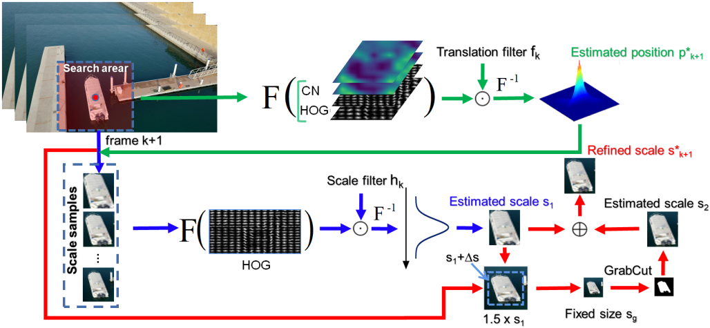
Figure 2: Overview of the proposed algorithm. The tracking task is decomposed into translation and scale estimation. At frame $k+1$, we first infer the target position $\textup{p}^{*}_{\textup{k}+1}$ using the translation filter $\textup{f}_{\textup{k}}$, and then predict the target scale $\textup{s}_{1}$ using the scale filter $\textup{h}_{\textup{k}}$. Finally, a segmentation-based scale refinement using the GrabCut is carried out, leading to a refined scale estimate $\textup{s}^{*}_{\textup{k+1}}$.

4.1.3 Update of appearance model

To improve robustness, the appearance model is adapted online [28, 24, 29] as follows:

$$\begin{split}\mathbf{\hat{x}}_{k}^{model}=(1-\alpha)\mathbf{\hat{x}}_{k-1}^{model}+\alpha\mathbf{\hat{x}}_{k-1}\end{split}$$ (13)

where $\alpha$ is the adaptation rate of the appearance model. $\mathbf{\hat{x}}_{k}^{model}$ instead of $\mathbf{\hat{x}}_{k}$ is then used to solve $\hat{\mathbf{g}}_{k}^{\ast}$.

4.1.4 Target localization

Spatial location of the target in the $(k+1)$th frame is localized by searching for the maximum value of response map $\mathbf{R}_{k+1}$ which is calculated by:

$$\begin{split}\mathbf{R}_{k+1}=\mathbf{F}^{-1}\left(\sum_{d=1}^{D}(\textup{conj}(\mathbf{\hat{z}}_{k+1}^{d})\odot\mathbf{\hat{g}}_{k}^{d})\right)\end{split}$$ (14)

where $\mathbf{\hat{z}}_{k+1}^{d}$ denotes the Fourier transform of extracted feature in the $(k+1)$th frame. Operator $\textup{conj}(.)$ denotes the complex conjugate operation.

4.2 Refine scale estimates with the GrabCut

As a graph cut [8] based method, GrabCut is is not only promising to specific images with known information but also effective to the natural images without any prior knowledge. It uses a Gaussian mixture model [49] to estimate the pixel color distribution of the object and background from a user specified bounding box around the segmented object, which is then used to construct a Markov random field [8] over the pixel labels with an energy function that prefers connected regions having the same label.

One disadvantage of it is the need for initial user interaction to initialize the segmentation process with a bounding box. Fortunately, in our scenario, we can adapt, by appropriately enlarging, the estimate of SSF to provide such an initial bounding box, which, hopefully, contains background as little as possible with the whole target being inside. Another disadvantage is, GrabCut may produce unacceptable results in the cases of low color contrast between the foreground and the background or high contrast among the foreground itself. Since we intend to exploit the accuracy of the GrabCut for refining, it is very important to refine the scale estimate of SSF only with acceptable segmentation by the GrabCut. Since for an effective SSF-based tracker the IoU (intersection over union) of the scale estimated by SSF with ground truth is supposed to be above a certain value in order to maintain the effectiveness of the appearance model, the IoU between the scale estimated by SSF and that derived from the GrabCut should be above a certain threshold as well if the segmentation was reliable. Therefore, this IoU between the SSF and the GrabCut above a certain threshold is used as the condition in this paper for conducting scale refinement to alleviate accumulating scale errors. The last but not least, although the GrabCut can achieve globally optimal result in polynomial time [57], it is still slow for UAV tracking if the input to the GrabCut is large. Therefore the input to the GrabCut is resized to a fixed and relatively small size to balance effectiveness and efficiency.

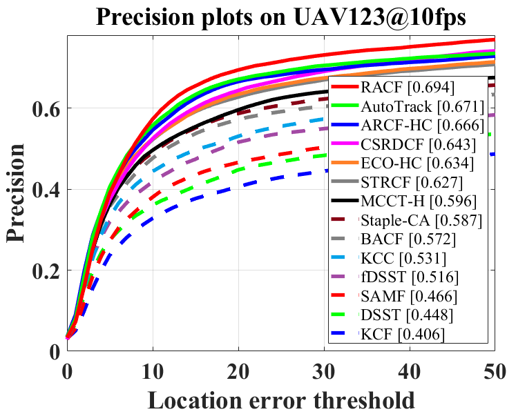
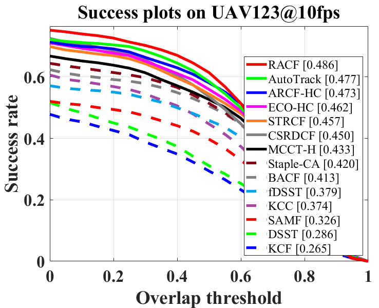
(a)

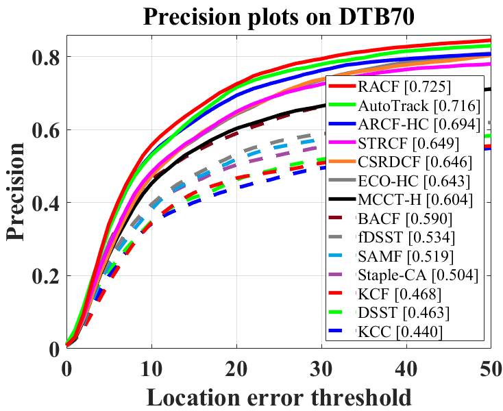
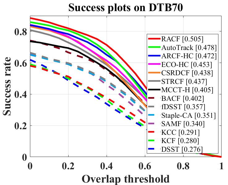
(b)

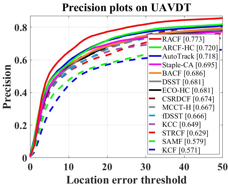
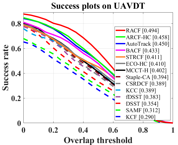
(c)

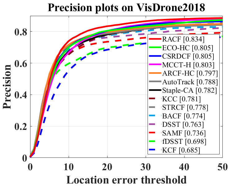
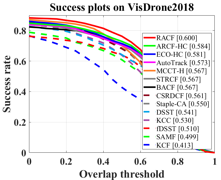
(d)

Figure 3: Overall performance of hand-crafted based trackers on (a) UAV123@10fps [50] (b) DTB70 [35](c) UAVDT [20] and (d) VisDrone2018 (VisDrone2018-test-dev) [72]. Precision and success rate for one-pass evaluation (OPE) [73] are used for evaluation. The precision at 20 pixels and area under curve (AUC) are used for ranking and marked in the precision plots and success plots respectively.

4.3 Our tracking framework

Fig. 2 illustrates the overview of the proposed algorithm for visual tracking. The translation filter $\textup{f}_{\textup{k}}$, formulated in the section 4.1, adapts to appearance changes of the target and its surrounding context for estimating translation. The 1D scale filter $\textup{h}_{\textup{k}}$ predicts scale variation of the target is the same as in [18, 24, 29]. The location of the target in the $(k+1)$th frame, denoted by $\textup{p}^{*}_{\textup{k}+1}$, is estimated by applying $\textup{f}_{\textup{k}}$ that has been updated in the $k$th frame to the detection sample extracted from the current frame at the last position $\textup{p}^{*}_{\textup{k}}$. Afterwards, $\textup{h}_{\textup{k}}$ is applied at multiple resolutions to estimate the scale of the target size, denoted by $\textup{s}_{1}$. At last, the proposed scale refinement is carried out. Firstly, an extended example is extracted centered at $\textup{p}^{*}_{\textup{k+1}}$ with size of $1.5\textup{s}_{1}$, which is associated a smaller bounding box of size $\textup{s}_{1}+\Delta\textup{s}$, $\Delta\textup{s}<0.5\textup{s}_{1}$, centered also at $\textup{p}^{*}_{\textup{k+1}}$. The extended example and the bounding box will be scaled to fixed sizes $\textup{s}_{g}$ and $\left[\frac{2}{3}(1+\Delta\textup{s}/\textup{s}_{1})\textup{s}_{g}\right]$, respectively, to make the input image and the initial bounding box for the GrabCut. Then the GrabCut is run to get the binary mask representing the foreground, the minimum bounding box of which, after resized, consists of the estimated scale $\textup{s}_{2}$ by the GrabCut. Finally, the refined scale is defined by

$$\begin{split}\textup{s}^{*}_{\textup{k+1}}=\left\{\begin{matrix}\textup{s}_{1},&\textup{if}\quad\mathbf{IoU}(\textup{s}_{1},\textup{s}_{2})>\sigma\\ \textup{s}_{2},&\textup{otherwise}\end{matrix}\right.,\end{split}$$ (15)

where $\mathbf{IoU}(\textup{s}_{1},\textup{s}_{2})$ computes the IoU between $\textup{s}_{1}$ and $\textup{s}_{2}$ and $\sigma$ is a predefined threshold.

Table 1: The proposed trackers with proposed components.

	RACF$\ominus\ominus$	RACF$\ominus$	RACF
Residue-aware regularization	✓	✓	✓
Spatial & temporal regularizations		✓	✓
Scale refinement			✓

5 Experiments

In this section, the proposed trackers with different components, summarized in Table 1, are exhaustively evaluated on four challenging UAV benchmarks, namely, UAV123@10fps [50], DTB70 [35], UAVDT [20] and Vistrone2018 [72]. UAV123@10fps is designed to investigate the impact of camera capture speed on tracking performance and constructed by down sampling the UAV123 benchmark [50] to 10 FPS from 30FPS. DTB70 composed of 70 UAV sequences primarily addresses the problem of severe UAV motion, but includes as well various cluttered scenes and objects with different sizes. UAVDT is mainly for vehicle tracking with various weather conditions, flying altitudes and camera views. Vistrone2018 (VisDrone2018-test-dev) is from the single object tracking challenge held in conjunction with the european conference on computer vision (ECCV2018), which focuses on evaluating tracking algorithms on drones. Our feature extractor is the same as in ARCF-HC, i.e., HOG and color name (CN) [29]. The evaluation experiments are conducted using MATLAB R2018a on a PC with an i7-7700K processor (3.7GHz), 32GB RAM and a NVIDIA GTX 960 GPU. For hyper parameters of RACF, we set $\eta=1$, $\theta=0.5$, $\tau=0.01$, $\lambda=0.55$. The spatial regularization weight is adapted from [36] with $\rho=1.5$. The parameters for scale refinement are set with $\textup{s}_{g}=52$, $\Delta\textup{s}=12$ and $\sigma=0.5$. All parameters settings are kept fixed for all videos in a dataset. ADMM iterations is set to 2. Code is available on: https://github.com/racf2021/racf

5.1 Comparison with hand-crafted based trackers

Thirteen state-of-the-art trackers based on hand-crafted features for comparison are: AutoTrack [38], ARCF-HC [29], STRCF [33], MCCT-H [69], KCC [66], ECO-HC [13], BACF [24], Staple-CA [52], CSRDCF [45], fDSST [16], KCF [28], DSST [19] and SAMF [41]. The precision and success plots on four benchmarks are shown in Fig. 3. Besides, the average performance in terms of frames per second (FPS) and precision is displayed in the Table 2.

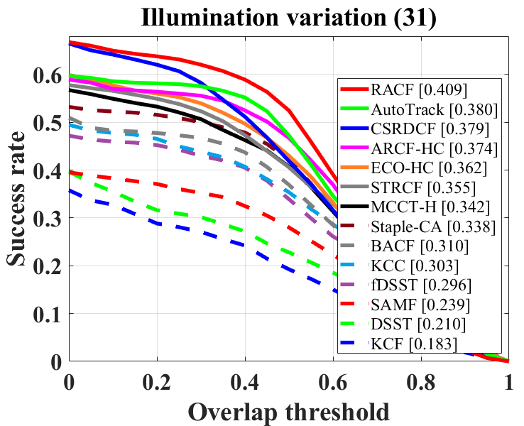
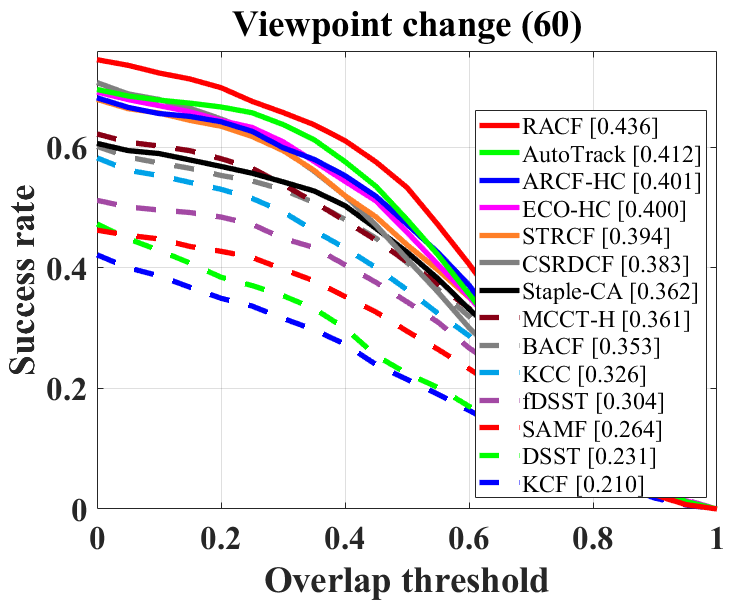
(a) UAV123@10fps

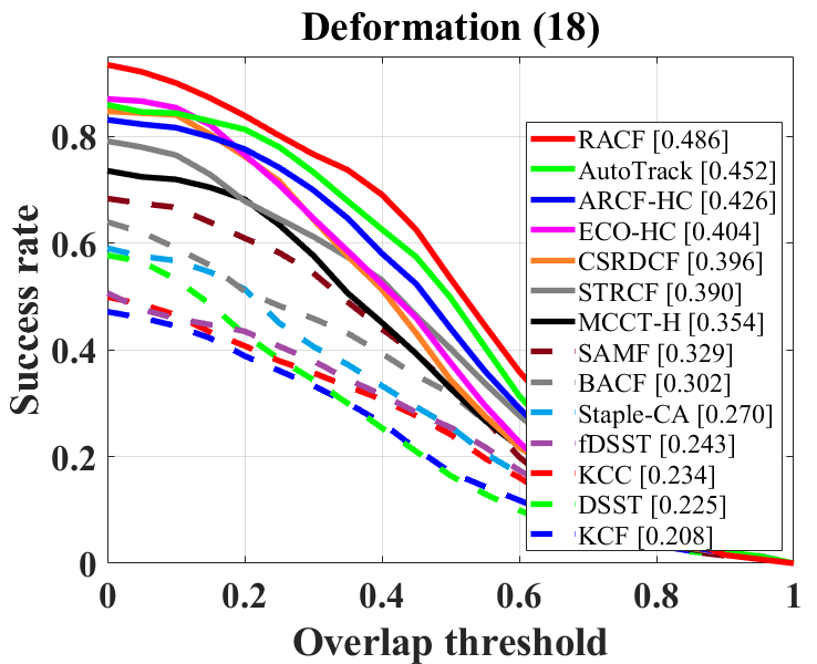
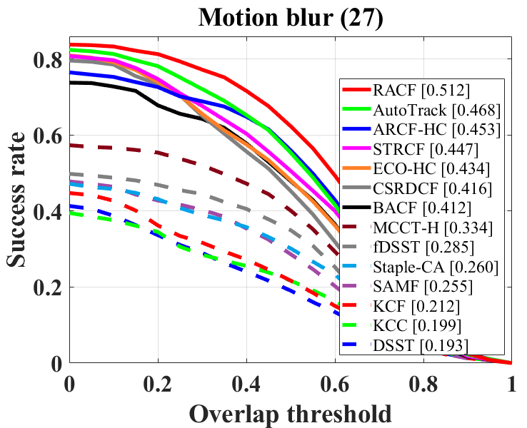
(b) DTB70

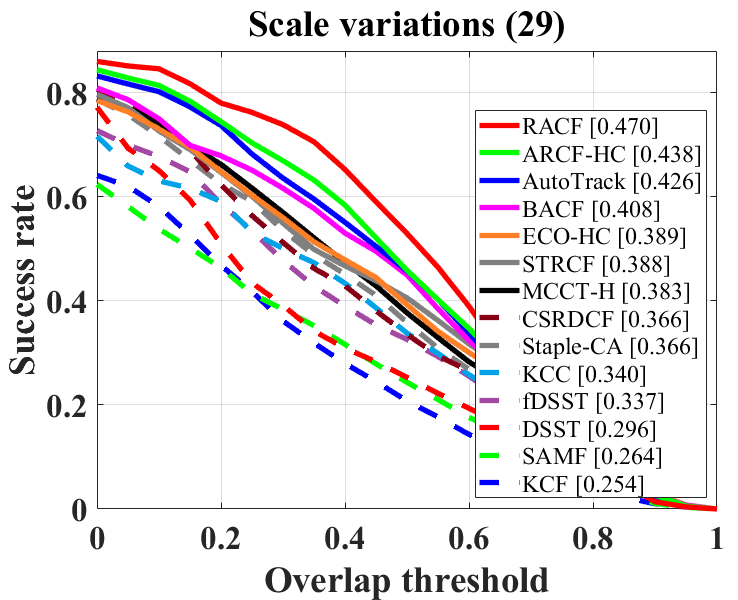
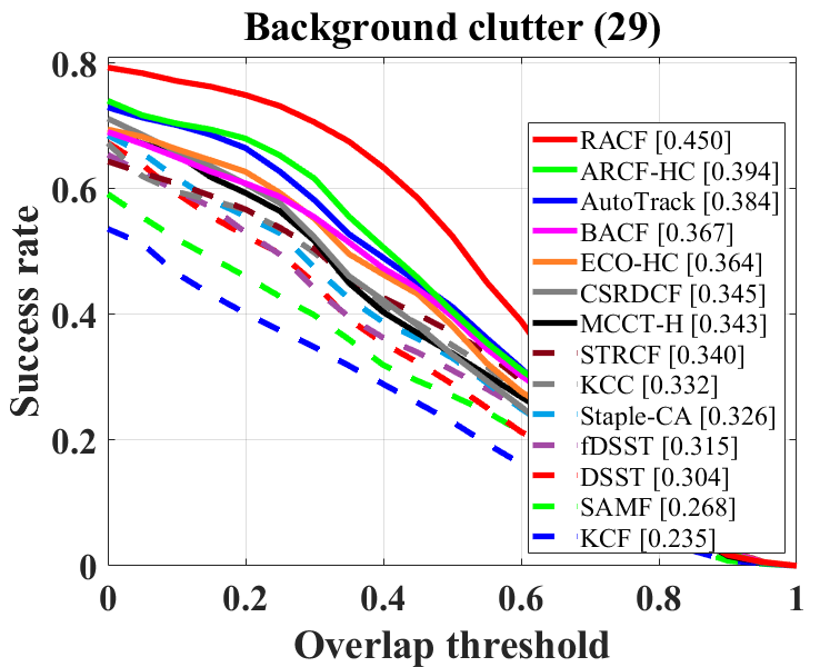
(c) UAVDT

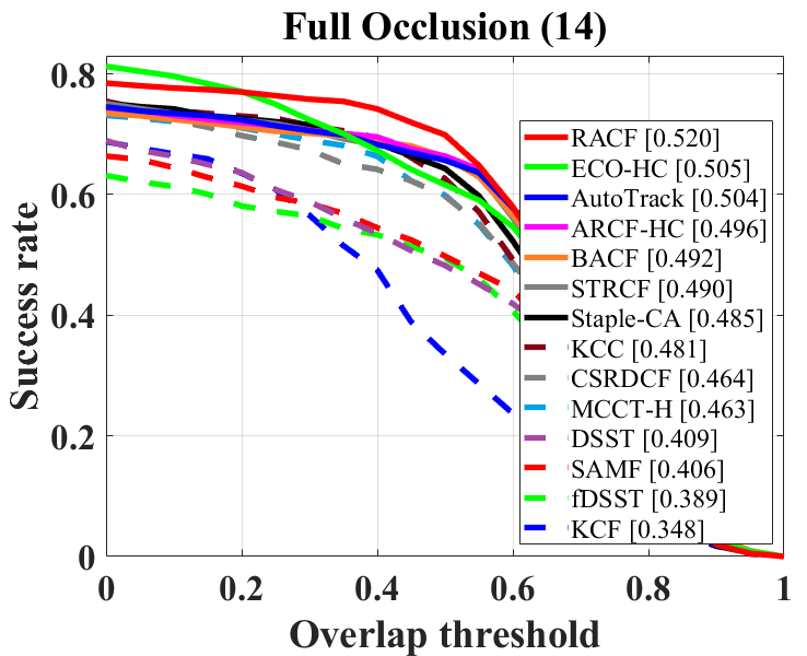
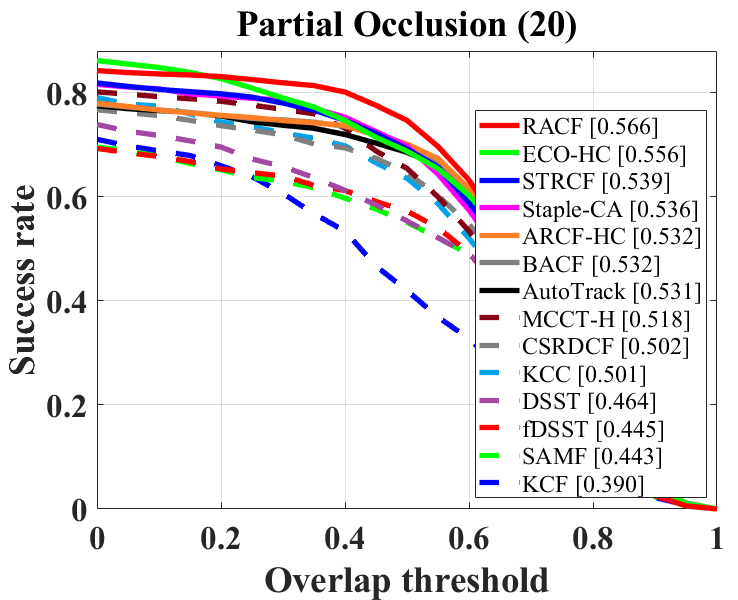
(d) VisDrone2018

Figure 4: Attribute-based comparison on illumination variation, viewpoint change, deformation, motion blur, scale variations, background clutter, full occlusion and partial occlusion.

Table 2: Average speed (FPS) and precision of hand-crafted based trackers on the four benchmarks. Red, green and blue respectively mean the first, second and third place. All the reported FPSs are evaluated on a single CPU. Noted that RACF$\ominus$ is the best real-time tracker.

	RACF	RACF$\ominus$	RACF$\ominus\ominus$	AutoTrack[38]	ARCF-HC[29]	KCF[28]	DSST[19]	BACF[24]	SAMF[41]	Staple-CA[52]	MCCT-H[69]	CSRDCF[45]	STRCF[33]	ECO-HC[13]	fDSST[16]	KCC[66]
Precision	75.7	74.3	73.0	72.3	71.9	53.3	58.9	65.3	57.5	64.2	66.8	69.2	67.1	68.8	60.4	60.0
FPS	26.3	36.2	36.3	43.2	25.2	545.8	88.3	45.1	9.6	52.7	50.9	10.6	23.0	62.1	164.7	35.2

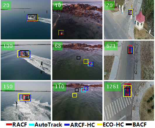
Figure 5: Qualitative evaluation on 3 video sequences from, respectively, UAV123@10fps, DTB70 and UAVDT (i.e. boat7, Gull1 and S1201). The results of AutoTrack, ARCF-HC, ECO-HC, BACF and our RACF are shown with different colors.

Overall performance evaluation: Fig. 3 shows the overall performance of RACF with the competing trackers on the four benchmarks. As can be seen, RACF outperforms all other trackers on all benchmarks. Specifically, on UAV123@10fps and DTB70, RACF outperforms the second tracker AutoTrack in (precision, AUC) with gains of (2.3%, 0.9%) and (0.9%, 2.7%) respectively. On UAVDT, RACF surpasses the second place, i.e, ARCF-HC, by a significant gain of (5.3%,3.6%). RACF also achieved the best performance on Vistrone2018, followed by ECO-HC with a gap of (2.9%, 1.6%). In terms of speed, we evaluate the average FPS of RACF, RACF$\ominus$ and RACF$\ominus\ominus$ with the competing trackers on the four benchmarks, the FPSs along with the average precisions are shown in Table 2. As can be seen, RACF$\ominus\ominus$ has already outperformed state-of-the-art trackers in precision and RACF$\ominus$ is the best real-time tracker (with a speed of $>$30FPS) on CPU. It also shows that RACF is near real-time even with scale refinement, and it makes little difference whether the spatial and temporal regularizations are used or not because $\tau\mathbf{I}$ and $\theta\mathbf{W}^{\textup{H}}\mathbf{W}$ in (6) are both diagonal matrices.
Attribute-based evaluation: The proposed RACF outperforms other hand-crafted based trackers in most attributes defined respectively in the four benchmarks. Examples of success plots are shown in Fig. 4. In the situations of deformation, viewpoint change and scale variations, RACF demonstrates a significant improvement over other trackers because the effectiveness of the proposed scale refinement in the corresponding benchmarks. All results are displayed in the supplementary materials.
Qualitative evaluation: Some qualitative tracking results of RACF and four top trackers are shown in Fig. 5. It can be seen that the scale estimates of RACF are more accurate in these examples with challenging viewpoint change, deformation and scale variations, justifying the effectiveness of the proposed method for refining scale estimates.

5.2 Comparison with deep-based trackers

The proposed RACF is also compared with fifteen state-of-the-art deep trackers, i.e., KYS [4], D3S [44], SiamR-CNN [65], PrDiMP18 [14], ASRCF [12], UDT+ [67], TADT [37], DeepSTRCF [33], MCCT [68], DSiam [24], ECO [13], ADNet [75], CFNet [63], MCPF [76] and CREST [59]. RACF achieves the second best precision and its CPU speed surpasses most GPU speeds on the UAVDT benchmark as shown in Table 3.

Table 3: Precision and speed (FPS) comparison between RACF and deep-based trackers on UAVDT [20]. * means GPU speed. Red, green and blue respectively mean the first, second and third place.

Tracker	Precision	FPS	Tracker	Precision	FPS
RACF	77.3	28.0	KYS [4]	79.8	18.6*
PrDiMP18 [14]	75.1	30.5*	D3S [44]	72.2	28.0*
SiamR-CNN [65]	66.5	4.6*	TADT [37]	67.7	19.1*
ASRCF [12]	70.0	14.2*	MCCT [68]	67.1	5.1*
UDT+ [67]	69.7	35.5*	ADNet [75]	68.3	4.7*
DeepSTRCF [33]	66.7	3.9*	ECO [13]	72.1	27.9*
MCPF [76]	66.0	0.4*	CFNet [63]	68.1	24.2*
DSiam [24]	70.4	9.3*	CREST [59]	64.9	2.5*

5.3 Ablation study

Table 4: Illustration of how success rate on DTB70 varies with the number of ADMM iterations in RACF$\ominus\ominus$ and the two baselines, i.e., BACF [24] and ARCF-HC [29]. The best success rates and the ones corresponding to default parameter settings are shown in red and underline, respectively.

	1	2	3	4	5	6	7	8	9	10	15	20	25
BACF[24]	23.113	40.201	41.016	40.864	40.695	40.866	40.845	40.577	40.555	40.72	40.773	40.433	40.615
ARCF-HC[29]	29.609	46.262	45.785	46.806	47.171	47.103	47.136	47.255	47.261	47.254	47.482	46.357	46.772
RACF$\ominus\ominus$	27.550	48.246	48.184	47.893	47.893	47.893	47.898	47.898	47.898	47.898	47.903	47.872	47.871

Table 5: AUCs and precisions on the four benchmarks. PRC is short for precision, and SR represents the scale refinement component. Red, green and blue respectively mean the first, second and third place.

	UAV123@10fps		DTB70		UAVDT		Vistrone2018		Avg.
Methods	AUC	RPC	AUC	RPC	AUC	RPC	AUC	RPC	AUC	RPC
ECO-HC[13] w/wo SR	46.2/47.7	63.4/66.0	45.3/46.0	64.3/64.6	41.0/46.5	68.1/72.7	58.1/58.8	80.5/81.2	47.7/49.8	69.1/71.1
ARCF-HC[29] w/wo SR	47.3/47.5	66.6/66.7	47.2/ 48.9	69.4/69.5	45.8/ 49.3	72.0/ 77.7	58.4/ 59.7	79.7/ 81.3	49.7/ 51.4	71.9/73.8
AutoTrack[38]w/wo SR	47.7/ 48.5	67.1/67.8	47.8/ 49.3	71.6/ 71.7	45.0/ 48.2	71.8/75.2	57.3/58.8	78.8/80.8	49.5/ 51.2	72.3/ 73.9
1-11 RACF $\ominus\ominus$	47.8	68.6	48.2	70.3	45.6	73.8	57.3	79.3	49.7	73.0
RACF $\ominus\quad$	47.8	69.1	48.5	70.7	46.6	75.3	59.2	82.1	50.5	74.3
RACF	48.6	69.4	50.5	72.5	49.4	77.3	60.0	83.4	52.1	75.6

Residue-aware regularization: To see how the number of ADMM iterations impacts the success rate of BACF, ARCF-HC and RACF$\ominus\ominus$, respectively, we evaluate the three trackers on DTB70 with varied ADMM iterations. The variations of success rate with respect to the number of ADMM iterations are shown in Table 4. As can be seen, RACF$\ominus\ominus$ obtains the highest success rate at iteration 2, BACF at iteration 3 and ARCF-HC at iteration 15, justifying that RACF$\ominus\ominus$ converges faster in average. We can also see that the fluctuations after iteration 2 are basically smaller in RACF$\ominus\ominus$ than in the others. To study the impact of $\eta$, the penalty of residue-aware regularization, we show in Tabel 6 the success rates of RACF$\ominus\ominus$ on DTB70 with respect to both $\eta$ and the number of ADMM iterations. As shown, RACF$\ominus\ominus$ achieves the highest success rate when $\eta=1.0$ at iteration 2. Notice that for each value of $\eta$ the highest success rate is obtained at iteration either 2 or 3, which conforms the fast convergence of the method.

Table 6: Illustration of how success rate on DTB70 varies with $\eta$ and the number of ADMM iterations in RACF$\ominus\ominus$. The best success rates are shown in red.

	0.2	0.4	0.6	0.8	1.0	1.2	1.4	1.6
1	28.782	27.933	27.927	27.083	27.550	27.342	27.672	28.295
2	46.590	46.977	47.903	48.098	48.246	46.971	47.031	47.203
3	47.039	46.879	47.712	47.544	48.184	47.603	46.595	46.572
4	47.018	46.843	47.752	47.522	47.893	47.190	46.651	46.595
5	47.018	46.843	47.752	47.522	47.893	47.190	46.651	46.595
6	47.018	46.806	47.752	47.522	47.893	47.190	46.700	46.595
7	47.018	46.806	47.752	47.521	47.898	47.190	46.700	46.595
8	47.018	46.806	47.752	47.521	47.898	47.190	46.700	46.595
9	47.018	46.806	47.752	47.521	47.898	47.189	46.700	46.587
10	47.018	46.796	47.839	47.521	47.898	47.189	46.700	46.587
15	47.035	46.773	47.843	47.521	47.903	47.152	46.660	46.591
20	47.029	46.773	47.640	47.526	47.872	47.155	46.660	46.544
25	47.029	46.747	47.590	47.540	47.871	47.155	46.680	46.541

Scale refinement, spatial and temporal regularizations: We incorporate the scale refinement (SR) component into three sate-of-the-art trackers, i.e, ECO-HC, ARCF-HC and AutoTrack, to validate its effectiveness and generality. The AUC and PRC, short for precision, on the four benchmarks are shown in Table 5. Equipped with SR, ECO-HC, ARCF-HC and AutoTrack acquire in average, respectively, gains of (2.1%, 2.0%), (1.7%, 1.9%) and (1.7%, 1.6%) in (AUC, PRC). The most significant improvements, specifically (5.5%, 4.6%), (3.5%, 5.7%) and (3.2%, 3.4%), are observed on UAVDT, for whose foreground and background are basically cars and roads and the GrabCut works well in these cases. The AUC and PRC of the proposed trackers are also shown in Table 5 beneath the dash line. As can be seen, in average, the SR component makes a gain of (1.6%, 1.3%) in (AUC, PRC), while the spatial and temporal regularizations make a gain of (0.8%, 1.3%), justifying the effectiveness of both components.

6 Conclusion

In this work, we proposed and evaluated the residue-aware correlation filters and the method of refining scale estimates with the GrabCut. The proposed RACF surpasses all sate-of-the-art hand-crafted based trackers in terms of precision and success rate in all the four UAV benchmarks and is comparable as well to many state-of-the-art deep-based trackers on UAVDT. The proposed scale refinement component can be easily incorporated into any tracking method with discriminative scale estimation to improve precision and accuracy.

References

- [1] Xiaofei Du A, Maximilian Allan B, Sebastian Bodenstedt C, Maier Hein D, Stefanie Speidel C, Alessio Dore E, and Danail Stoyanov A. Patch-based adaptive weighting with segmentation and scale (pawss) for visual tracking in surgical video. Medical Image Analysis, 57:120–135, 2019.
- [2] Chad Aeschliman, Johnny Park, and Avinash C. Kak. A probabilistic framework for joint segmentation and tracking. In 2010 IEEE Computer Society Conference on Computer Vision and Pattern Recognition, pages 1371–1378, 2010.
- [3] David Balduzzi, Marcus Frean, Lennox Leary, J P Lewis, Kurt Wan-Duo Ma, and Brian McWilliams. The shattered gradients problem: if resnets are the answer, then what is the question? In ICML’17 Proceedings of the 34th International Conference on Machine Learning - Volume 70, pages 342–350, 2017.
- [4] Goutam Bhat, Martin Danelljan, Luc Van Gool, and Radu Timofte. Know your surroundings: Exploiting scene information for object tracking. In ECCV (23), pages 205–221, 2020.
- [5] Adel Bibi, Matthias Mueller, and Bernard Ghanem. Target response adaptation for correlation filter tracking. 2016.
- [6] David S Bolme, J Ross Beveridge, Bruce A Draper, and Yui Man Lui. Visual object tracking using adaptive correlation filters. In 2010 IEEE computer society conference on computer vision and pattern recognition, pages 2544–2550. IEEE, 2010.
- [7] Stephen Boyd, Neal Parikh, Eric Chu, Borja Peleato, and Jonathan Eckstein. Distributed optimization and statistical learning via the alternating direction method of multipliers. Foundations & Trends in Machine Learning, 3(1):1–122, 2010.
- [8] Yuri Boykov and Gareth Funka-Lea. Graph cuts and efficient n-d image segmentation. International Journal of Computer Vision, 70(2):109–131, 2006.
- [9] William L Briggs, Van Emden Henson, and Steve F McCormick. A multigrid tutorial. SIAM, 2000.
- [10] Ken Chatfield, Victor S. Lempitsky, Andrea Vedaldi, and Andrew Zisserman. The devil is in the details: an evaluation of recent feature encoding methods. In British Machine Vision Conference 2011, pages 1–12, 2011.
- [11] Xi Chen, Zuoxin Li, Ye Yuan, Gang Yu, Jianxin Shen, and Donglian Qi. State-aware tracker for real-time video object segmentation. In 2020 IEEE/CVF Conference on Computer Vision and Pattern Recognition (CVPR), pages 9384–9393, 2020.
- [12] Kenan Dai, Dong Wang, Huchuan Lu, Chong Sun, and Jianhua Li. Visual tracking via adaptive spatially-regularized correlation filters. In 2019 IEEE/CVF Conference on Computer Vision and Pattern Recognition (CVPR), pages 4670–4679, 2019.
- [13] Martin Danelljan, Goutam Bhat, Fahad Shahbaz Khan, and Michael Felsberg. Eco: Efficient convolution operators for tracking. In 2017 IEEE Conference on Computer Vision and Pattern Recognition (CVPR), pages 6931–6939, 2017.
- [14] Martin Danelljan, Luc Van Gool, and Radu Timofte. Probabilistic regression for visual tracking. In 2020 IEEE/CVF Conference on Computer Vision and Pattern Recognition (CVPR), pages 7183–7192, 2020.
- [15] Martin Danelljan, Gustav Hager, Fahad Shahbaz Khan, and Michael Felsberg. Learning spatially regularized correlation filters for visual tracking. In 2015 IEEE International Conference on Computer Vision (ICCV), pages 4310–4318, 2015.
- [16] Martin Danelljan, Gustav Hager, Fahad Shahbaz Khan, and Michael Felsberg. Adaptive decontamination of the training set: A unified formulation for discriminative visual tracking. In 2016 IEEE Conference on Computer Vision and Pattern Recognition (CVPR), pages 1430–1438, 2016.
- [17] Martin Danelljan, Gustav Hager, Fahad Shahbaz Khan, and Michael Felsberg. Convolutional features for correlation filter based visual tracking. In 2015 IEEE International Conference on Computer Vision Workshop (ICCVW), 2016.
- [18] Martin Danelljan, Gustav Hager, Fahad Shahbaz Khan, and Michael Felsberg. Discriminative scale space tracking. IEEE Transactions on Pattern Analysis and Machine Intelligence, 39(8):1561–1575, 2017.
- [19] Martin Danelljan, Gustav Häger, Fahad Shahbaz Khan, and Michael Felsberg. Accurate scale estimation for robust visual tracking. In British Machine Vision Conference, 2014.
- [20] Dawei Du, Yuankai Qi, Hongyang Yu, Yifan Yang, Kaiwen Duan, Guorong Li, Weigang Zhang, Qingming Huang, and Qi Tian. The unmanned aerial vehicle benchmark: Object detection and tracking. In Proceedings of the European Conference on Computer Vision (ECCV), pages 375–391, 2018.
- [21] Stefan Duffner and Christophe Garcia. Pixeltrack: a fast adaptive algorithm for tracking non-rigid objects. In Proceedings of the IEEE international conference on computer vision, pages 2480–2487, 2013.
- [22] Changhong Fu, Fuling Lin, Yiming Li, and Guang Chen. Correlation filter-based visual tracking for uav with online multi-feature learning. Remote Sensing, 11(5), 2019.
- [23] Changhong Fu, Juntao Xu, Fuling Lin, Fuyu Guo, and Zhijun Zhang. Object saliency-aware dual regularized correlation filter for real-time aerial tracking. IEEE Transactions on Geoscience and Remote Sensing, page 12, 2020.
- [24] Hamed Kiani Galoogahi, Ashton Fagg, and Simon Lucey. Learning background-aware correlation filters for visual tracking. In 2017 IEEE International Conference on Computer Vision (ICCV), 2017.
- [25] Martin Godec, Peter M. Roth, and Horst Bischof. Hough-based tracking of non-rigid objects. In 2011 International Conference on Computer Vision, pages 81–88, 2011.
- [26] Kaiming He, Xiangyu Zhang, Shaoqing Ren, and Jian Sun. Deep residual learning for image recognition. In Proceedings of the IEEE conference on computer vision and pattern recognition, pages 770–778, 2016.
- [27] Yujie He, Changhong Fu, Fuling Lin, Yiming Li, and Peng Lu. Towards robust visual tracking for unmanned aerial vehicle with tri-attentional correlation filters. arXiv preprint arXiv:2008.00528, 2020.
- [28] Joao F. Henriques, Rui Caseiro, Pedro Martins, and Jorge Batista. High-speed tracking with kernelized correlation filters. IEEE Transactions on Pattern Analysis & Machine Intelligence, 37(3):583–596, 2015.
- [29] Ziyuan Huang, Changhong Fu, Yiming Li, Fuling Lin, and Peng Lu. Learning aberrance repressed correlation filters for real-time uav tracking. In 2019 IEEE/CVF International Conference on Computer Vision (ICCV), pages 2891–2900, 2019.
- [30] Mücahit Karaduman, Ahmet Cevahir Cinar, and Haluk Eren. Uav traffic patrolling via road detection and tracking in anonymous aerial video frames. Journal of Intelligent and Robotic Systems, 95(2):675–690, 2019.
- [31] Kenji Kawaguchi. Deep learning without poor local minima. In Advances in Neural Information Processing Systems (NeurIPS), volume 29, pages 586–594, 2016.
- [32] Fan Li, Changhong Fu, Fuling Lin, Yiming Li, and Peng Lu. Training-set distillation for real-time uav object tracking. In 2020 IEEE International Conference on Robotics and Automation (ICRA), pages 9715–9721, 2020.
- [33] Feng Li, Cheng Tian, Wangmeng Zuo, Lei Zhang, and Ming-Hsuan Yang. Learning spatial-temporal regularized correlation filters for visual tracking. In 2018 IEEE/CVF Conference on Computer Vision and Pattern Recognition, pages 4904–4913, 2018.
- [34] Peixia Li, Boyu Chen, Wanli Ouyang, Dong Wang, Xiaoyun Yang, and Huchuan Lu. Gradnet: Gradient-guided network for visual object tracking. In 2019 IEEE/CVF International Conference on Computer Vision (ICCV), pages 6162–6171, 2019.
- [35] Siyi Li and Dit Yan Yeung. Visual object tracking for unmanned aerial vehicles: A benchmark and new motion models. In Proceedings of the 31st AAAI Conference on Artificial Intelligence, pages 4140–4146, 2017.
- [36] Shui-wang Li, Qian-bo Jiang, Qi-jun Zhao, Li Lu, and Zi-liang Feng. Asymmetric discriminative correlation filters for visual tracking. Frontiers of Information Technology & Electronic Engineering, 21(10):1467–1484, 2020.
- [37] Xin Li, Chao Ma, Baoyuan Wu, Zhenyu He, and Ming-Hsuan Yang. Target-aware deep tracking. In 2019 IEEE/CVF Conference on Computer Vision and Pattern Recognition (CVPR), pages 1369–1378, 2019.
- [38] Yiming Li, Changhong Fu, Fangqiang Ding, Ziyuan Huang, and Geng Lu. Autotrack: Towards high-performance visual tracking for uav with automatic spatio-temporal regularization. In 2020 IEEE/CVF Conference on Computer Vision and Pattern Recognition (CVPR), pages 11923–11932, 2020.
- [39] Yiming Li, Changhong Fu, Fangqiang Ding, Ziyuan Huang, and Jia Pan. Augmented memory for correlation filters in real-time uav tracking. arXiv preprint arXiv:1909.10989, 2019.
- [40] Yiming Li, Changhong Fu, Ziyuan Huang, Yinqiang Zhang, and Jia Pan. Keyfilter-aware real-time uav object tracking. In 2020 IEEE International Conference on Robotics and Automation (ICRA), pages 193–199, 2020.
- [41] Yang Li and Jianke Zhu. A scale adaptive kernel correlation filter tracker with feature integration. In European Conference on Computer Vision, pages 254–265, 2014.
- [42] Fuling Lin, Changhong Fu, Yujie He, Fuyu Guo, and Qian Tang. Bicf: Learning bidirectional incongruity-aware correlation filter for efficient uav object tracking. In 2020 IEEE International Conference on Robotics and Automation (ICRA), pages 2365–2371, 2020.
- [43] Shanggang Lin, Matthew A. Garratt, and Andrew J. Lambert. Monocular vision-based real-time target recognition and tracking for autonomously landing an uav in a cluttered shipboard environment. Autonomous Robots, 41(4), 2016.
- [44] Alan Lukezic, Jiri Matas, and Matej Kristan. D3s – a discriminative single shot segmentation tracker. In 2020 IEEE/CVF Conference on Computer Vision and Pattern Recognition (CVPR), pages 7133–7142, 2020.
- [45] Alan Lukezic, Tomas Vojir, Luka Cehovin Zajc, Jiri Matas, and Matej Kristan. Discriminative correlation filter with channel and spatial reliability. In 2017 IEEE Conference on Computer Vision and Pattern Recognition (CVPR), pages 4847–4856, 2017.
- [46] Chao Ma, Jia-Bin Huang, Xiaokang Yang, and Ming-Hsuan Yang. Hierarchical convolutional features for visual tracking. In 2015 IEEE International Conference on Computer Vision (ICCV), pages 3074–3082, 2015.
- [47] Seyed Mojtaba Marvasti-Zadeh, Hossein Ghanei-Yakhdan, and Shohreh Kasaei. Rotation-aware discriminative scale space tracking. In 2019 27th Iranian Conference on Electrical Engineering (ICEE), 2019.
- [48] Seyed Mojtaba Marvasti-Zadeh, Hossein Ghanei-Yakhdan, and Shohreh Kasaei. Efficient scale estimation methods using lightweight deep convolutional neural networks for visual tracking. Neural Computing and Applications, pages 1–16, 2021.
- [49] G. J. Mclachlan and K. E. Basford. Mixture models: Inference and applications to clustering. Applied Statistics, 38(2), 1988.
- [50] Matthias Mueller, Neil Smith, and Bernard Ghanem. A benchmark and simulator for uav tracking. Far East Journal of Mathematical Sciences, 2(2):445–461, 2016.
- [51] Matthias Mueller, Neil Smith, and Bernard Ghanem. Context-aware correlation filter tracking. In IEEE Conference on Computer Vision & Pattern Recognition, 2017.
- [52] Matthias Mueller, Neil Smith, and Bernard Ghanem. Context-aware correlation filter tracking. In 2017 IEEE Conference on Computer Vision and Pattern Recognition (CVPR), pages 1387–1395, 2017.
- [53] Stephen G Nash. A multigrid approach to discretized optimization problems. Optimization Methods and Software, 14(1-2):99–116, 2000.
- [54] Miguel Olivares-Mendez, Changhong Fu, Philippe Ludivig, Tegawendé Bissyandé, Somasundar Kannan, Maciej Zurad, Arun Annaiyan, Holger Voos, and Pascual Campo. Towards an autonomous vision-based unmanned aerial system against wildlife poachers. Sensors, 2015.
- [55] A. Emin Orhan and Xaq Pitkow. Skip connections eliminate singularities. In International Conference on Learning Representations, 2018.
- [56] Xiaofeng Ren and J. Malik. Tracking as repeated figure/ground segmentation. In 2007 IEEE Conference on Computer Vision and Pattern Recognition, pages 1–8, 2007.
- [57] C. Rother. Grabcut : Interactive foreground extraction using iterated graph cut. Acm Trans Graph, 23, 2004.
- [58] Jack Sherman and Winifred J Morrison. Adjustment of an inverse matrix corresponding to a change in one element of a given matrix. The Annals of Mathematical Statistics, 21(1):124–127, 1950.
- [59] Yibing Song, Chao Ma, Lijun Gong, Jiawei Zhang, Rynson WH Lau, and Ming-Hsuan Yang. Crest: Convolutional residual learning for visual tracking. In Proceedings of the IEEE International Conference on Computer Vision, pages 2555–2564, 2017.
- [60] Mingjie Sun, Jimin Xiao, Eng Gee Lim, Bingfeng Zhang, and Yao Zhao. Fast template matching and update for video object tracking and segmentation. In 2020 IEEE/CVF Conference on Computer Vision and Pattern Recognition (CVPR), pages 10791–10799, 2020.
- [61] Richard Szeliski. Locally adapted hierarchical basis preconditioning. In ACM SIGGRAPH 2006 Papers, pages 1135–1143. 2006.
- [62] Yi-Hsuan Tsai, Ming-Yu Liu, Deqing Sun, Ming-Hsuan Yang, and Jan Kautz. Learning binary residual representations for domain-specific video streaming. In Proceedings of the AAAI Conference on Artificial Intelligence, volume 32, 2018.
- [63] Jack Valmadre, Luca Bertinetto, João F. Henriques, Andrea Vedaldi, and Philip H. S. Torr. End-to-end representation learning for correlation filter based tracking. 2017.
- [64] Andrea Vedaldi and Brian Fulkerson. Vlfeat: an open and portable library of computer vision algorithms. In Proceedings of the 18th ACM international conference on Multimedia, pages 1469–1472, 2010.
- [65] Paul Voigtlaender, Jonathon Luiten, Philip H.S. Torr, and Bastian Leibe. Siam r-cnn: Visual tracking by re-detection. In 2020 IEEE/CVF Conference on Computer Vision and Pattern Recognition (CVPR), pages 6578–6588, 2020.
- [66] Chen Wang, Le Zhang, Lihua Xie, and Junsong Yuan. Kernel cross-correlator. In The Thirty-Second AAAI Conference on Artificial Intelligence (AAAI-18), 2018.
- [67] Ning Wang, Yibing Song, Chao Ma, Wengang Zhou, Wei Liu, and Houqiang Li. Unsupervised deep tracking. In 2019 IEEE/CVF Conference on Computer Vision and Pattern Recognition (CVPR), pages 1308–1317, 2019.
- [68] Ning Wang, Wengang Zhou, Qi Tian, Richang Hong, and Houqiang Li. Multi-cue correlation filters for robust visual tracking. In 2018 IEEE/CVF Conference on Computer Vision and Pattern Recognition (CVPR), 2018.
- [69] Ning Wang, Wengang Zhou, Qi Tian, Richang Hong, Meng Wang, and Houqiang Li. Multi-cue correlation filters for robust visual tracking. In 2018 IEEE/CVF Conference on Computer Vision and Pattern Recognition, pages 4844–4853, 2018.
- [70] Qiang Wang, Li Zhang, Luca Bertinetto, Weiming Hu, and Philip H.S. Torr. Fast online object tracking and segmentation: A unifying approach. In 2019 IEEE/CVF Conference on Computer Vision and Pattern Recognition (CVPR), pages 1328–1338, 2019.
- [71] Z. L Wang and B. G Cai. A comparison study of adaptive scale estimation in correlation filter-based visual tracking methods. Robotics & Biomimetics, 4(1):11, 2017.
- [72] Longyin Wen, Pengfei Zhu, Dawei Du, and et al. Visdrone-sot2018: The vision meets drone single-object tracking challenge results. In Proceedings of the European Conference on Computer Vision (ECCV) Workshops, pages 469–495, 2018.
- [73] Yi Wu, Jongwoo Lim, and Ming Hsuan Yang. Online object tracking: A benchmark. In Computer Vision & Pattern Recognition, 2013.
- [74] Chi Yuan, Zhixiang Liu, and Youmin Zhang. Aerial images-based forest fire detection for firefighting using optical remote sensing techniques and unmanned aerial vehicles. Journal of Intelligent & Robotic Systems, 2017.
- [75] Sangdoo Yun, Jongwon Choi, Youngjoon Yoo, Kimin Yun, and Jin Young Choi. Action-decision networks for visual tracking with deep reinforcement learning. In IEEE Conference on Computer Vision & Pattern Recognition, 2017.
- [76] Tianzhu Zhang, Changsheng Xu, and Ming Hsuan Yang. Multi-task correlation particle filter for robust object tracking. In 2017 IEEE Conference on Computer Vision and Pattern Recognition (CVPR), 2017.