Abstract

Inference and testing in general point process models such as the Hawkes model is predominantly based on asymptotic approximations for likelihood-based estimators and tests. As an alternative, and to improve finite sample performance, this paper considers bootstrap-based inference for interval estimation and testing. Specifically, for a wide class of point process models we consider a novel bootstrap scheme labeled ‘fixed intensity bootstrap’ (FIB), where the conditional intensity is kept fixed across bootstrap repetitions. The FIB, which is very simple to implement and fast in practice, extends previous ideas from the bootstrap literature on time series in discrete time, where the so-called ‘fixed design’ and ‘fixed volatility’ bootstrap schemes have shown to be particularly useful and effective. We compare the FIB with the classic recursive bootstrap, which is here labeled ‘recursive intensity bootstrap’ (RIB). In RIB algorithms, the intensity is stochastic in the bootstrap world and implementation of the bootstrap is more involved, due to its sequential structure. For both bootstrap schemes, we provide new bootstrap (asymptotic) theory which allows to assess bootstrap validity, and propose a ‘non-parametric’ approach based on resampling time-changed transformations of the original waiting times. We also establish the link between the proposed bootstraps for point process models and the related autoregressive conditional duration (ACD) models. Lastly, we show effectiveness of the different bootstrap schemes in finite samples through a set of detailed Monte Carlo experiments, and provide applications to both financial data and social media data to illustrate the proposed methodology.

Keywords: Self-exciting point processes; conditional intensity; bootstrap inference; Hawkes process; autoregressive conditional duration models.

JEL Classification: C32.

1 Introduction

Point processes are well-known to be useful tools to characterize dynamics of event occurrence times. This includes the homogeneous Poisson process where the intensity process is constant over time, the inhomogeneous Poisson process, where the intensity is a deterministic (or strictly exogenous) time-varying function, as well as the class of ‘self-exciting’ point processes, such as the well-known and much applied Hawkes process. In particular, for the Hawkes process, the conditional intensity process depends on all past history of the events and thereby allows for (exponential or fractional) memory features, similar to autoregressive or fractional time-series processes in discrete time series econometrics. The self-exciting class of models, which are the focus of this paper, were originally proposed for modelling earthquake sequences; see Ogata (1988) and the references therein. Later, they have been put to use in a wide range of applications such as financial transactions (Bowsher, 2007; Bauwens and Hautsch, 2009), financial contagion (Aït-Sahalia et al., 2015), monetary policy (Dolado and María-Dolores, 2002), criminal fights and relations (Mohler et al., 2011), forecasting electricity price spikes (Clements et al., 2015) and the rich literature on social network information diffusion (Rizoiu et al., 2017), among others. Hawkes processes are also closely related to the class of autoregressive conditional duration [ACD] models of Engle and Russell (1998), which are well known and much used in financial economics; see Sections 2 and 6 below for the relation between the two classes of processes.

Inference for self-exciting point process models is generally performed through classic, likelihood-based asymptotic inference and testing, as originally discussed in Ogata (1978). However, see e.g. Reinhart (2018) and Wang et al. (2010), the finite sample performance of asymptotic inference is not always satisfactory. This is in general the case because the finite sample distributions of the estimators are often very skewed and far from the Gaussian asymptotic distribution.

In this framework, a key motivation for the results presented in the paper is to provide a simple to implement, and theoretically well-grounded, bootstrap approach to inference in self-exciting point process models. We do this by providing six main contributions.

The first contribution is to propose a novel (non-)parametric bootstrap scheme for such point process models, which we label as ‘fixed intensity bootstrap’ (FIB). The FIB is simple and fast to implement in practice – particularly so when compared to existing (recursive) applications of the bootstrap. The key difference between the new and the classic bootstrap schemes is how to generate the sequence of waiting times in the bootstrap world. Specifically, while for standard, recursive bootstrap schemes, the bootstrap event times are generated recursively through the past bootstrap events, for the novel bootstrap scheme the bootstrap event times are generated using a ‘fixed’ conditional intensity function, which entirely depends on the event times in the original world. Therefore, the FIB contrasts with existing implementations of the bootstrap, see e.g. Embrechts et al. (2011) and Sarma et al. (2011), which utilize a (possibly highly complex and time consuming) sequential update of the bootstrap conditional intensities.

The second contribution is to provide bootstrap (first-order) asymptotic theory, including establishing bootstrap validity for inference and testing in point process models for both the novel (FIB) bootstrap and for the classic recursive bootstrap (for which no theory exists in the literature). We show that the bootstrap based on the FIB is valid under regularity conditions which are milder than those required for validity of recursive bootstrap schemes (hereafter, RIB).

The third contribution is to introduce novel ‘non-parametric’ implementations of the FIB and RIB schemes, which are based on resampling time-changed transformations of the original waiting times, rather than generating the (transformed) waiting times through a parametric model (usually the exponential distribution), as is in the literature. These implementations are likely to be robust to model misspecifications which generate non-exponential transformed waiting times. We show how to scale the original time-changed waiting times properly and to resample them; we also show that, in the homogeneous case, validity of the implied bootstrap follows from a time-change functional central limit theorem derived by Billingsley (1968) which, as far as we are aware, has never been applied to the bootstrap of self-exciting point process models.

The fourth contribution of the paper is a detailed Monte Carlo simulation study on the performance of the bootstrap for self-exciting Hawkes processes. Possibly due to the high computational costs involved in the implementation of a simulation study for the bootstrap in this framework, to the best of our knowledge studies like ours have not been attempted in the literature. We show that for Hawkes processes with exponential kernels, the coverage probabilities of confidence intervals based on the Gaussian asymptotic approximation may be well below the nominal level. In contrast, the bootstrap is able to correct this and, in particular, FIB implementations are particularly well performing in terms of coverage probabilities.

The fifth contribution is to provide two real data examples where we illustrate the key differences between asymptotic and the various bootstrap inference methods in applications. The first refers to the problem of modeling and predicting extreme financial results, see Embrechts et al. (2011). We use this example, including the data sample considered in Embrechts et al. (2011), to compare the outcome of the four different bootstrap schemes discussed in the paper. The second example is based on social media data and considers the flows of tweets and re-tweets proceeding and following a political announcement. Specifically, using recent tweets related to the COVID-19 pandemic in Denmark, we show how bootstrap-based inference is able to detect structural breaks (in the mean intensity as well as in the decay rate of intensity) induced by the announcement, which may not be detected based on asymptotic inference.

Sixth, we discuss the link between the proposed bootstraps based on the point process representation and bootstrap inference for autoregressive conditional duration (ACD) models. We establish the relation between our proposed bootstrap schemes and bootstrap algorithms based on the ACD representation. Specifically, we show that our recursive bootstrap corresponds to a residual-based bootstrap in the ACD world (as discussed e.g. in Perera and Silvapulle, 2021), with the crucial difference that the number of events generated through our scheme is random, rather than being fixed. This is a key improvement, as our bootstrap ensures that the sum of the bootstrap waiting times always cover the original time interval. We also show that residual-based implementation of the bootstrap in the ACD world corresponds to our proposed non-parametric bootstrap with re-sampling based on the (estimated) transformed waiting times. Finally, we discuss the relation between our proposed fixed intensity bootstrap and a bootstrap in the ACD framework, which is novel in the literature, where the conditional duration in the bootstrap world is fixed to the estimated conditional duration in the original sample.

Structure of the paper

The paper is organized as follows. In Section 2 likelihood-based analysis for point processes inference is presented, and in Section 3 the novel fixed intensity, as well as the recursive intensity, bootstraps are discussed, with theory and validity results in Section 4. Non-parametric bootstrap is discussed in Section 5, and the relation between our bootstraps and the bootstraps for ACD models is discussed in Section 6. Section 7 provides a Monte Carlo study of the different schemes. Section 8 contains two empirical illustrations, and Section 9 concludes. All proofs are contained in the Appendix.

Notation

We use the counting process $N(t)$ to characterize the total number of events occurring before and including time $t$, with $N(s,t]$ and $N[s,t)$ the numbers of events in the interval $(s,t]$ and $[s,t)$, respectively, for $s<t$. For a right-continuous natural filtration $(\mathcal{F}_{t})_{t\in\mathbb{R}}$ of a continuous time stochastic process, we denote by $\mathcal{F}_{t-}$ the left limit of $\mathcal{F}_{t}$, which contains all the information before but not including time $t$. We use $\mathbb{I}(\cdot)$ to denote the indicator function, and define $\mathbb{R}^{+}:=(0,\infty)$ and $\mathbb{R}_{+}:=[0,\infty)$. For $x\in\mathbb{R}$, $\lfloor x\rfloor:=\max_{z\in\mathbb{Z}}\{z\leq x\}$. For the bootstrap, as is standard, we denote by $P^{\ast}$ the probability measure induced by the bootstrap; expectation and variance computed under $P^{\ast}$ are denoted by $E^{\ast}$ and $V^{\ast}$, respectively. For a sequence $X_{T}^{\ast}$ computed on the bootstrap data, $X_{T}^{\ast}\overset{p^{\ast}}{\rightarrow}_{p}0$ or $X_{T}^{\ast}=o_{p}^{\ast}(1)$, in probability, denote that $P^{\ast}(|X_{T}^{\ast}|>\epsilon)\rightarrow 0$ in probability for any $\epsilon>0$; $X_{T}^{\ast}=O_{p}^{\ast}(1)$, in probability, denotes that there exists a $c>0$ such that $P^{\ast}(|X_{T}^{\ast}|>c)\rightarrow 0$ in probability; with $X_{T}^{\ast}\overset{d^{\ast}}{\rightarrow}_{p}X$ (weak convergence in probability) we mean that $E^{\ast}(g(X_{T}^{\ast}))\overset{p}{\rightarrow}E(g(X))$ for all continuous bounded functions $g$, in each case as $T\rightarrow\infty$. Finally, $\mathcal{N}$ denotes a Gaussian random variable and, for $\mu>0$, $\mathcal{E}(\mu)$ denotes an exponential random variable with mean $1/\mu$.

2 Likelihood-based analysis of the point process

We discuss here likelihood-based estimation for a general class of point process models. For later use when establishing asymptotic validity of the bootstrap, we state explicit sufficient conditions for classic likelihood-based asymptotic theory. Precisely, and as in Ogata (1978), we establish consistency and limiting distributions of likelihood-based estimators, as well as the related (likelihood ratio) test statistics.

2.1 The model

By assumption, the observed event times are realizations from a univariate point process, i.e. a collection $\{t_{i}\}_{i=1}^{\infty}$, $t_{i}>0$, of stochastic event times with associated waiting times (or durations), $w_{i}:=t_{i}-t_{i-1}$, for $i=1,2,...$ with $t_{0}:=0$; see e.g. Daley and Vere-Jones (2003) for an introduction to point processes. The point process can be equivalently characterized by the continuous-time counting process

$$N(t):=\sum_{i\geq 1}\mathbb{I}(t_{i}\leq t),$$ (2.1)

for $t\geq 0$, with associated filtration $(\mathcal{F}_{t}),t\geq 0$ where $\mathcal{F}_{t}$ is the $\sigma$-field generated by $\{N(s),s\leq t\}$.

In addition, and as used here predominantly, a regular point process is uniquely defined by its conditional intensity process, $\lambda(t)$, $t\geq 0$, which captures the instantaneous conditional probability of event occurrences and is defined as

$$\lambda(t):=\lim_{\delta\rightarrow 0^{+}}\frac{1}{\delta}P(N[t,t+\delta)>0|\mathcal{F}_{t-}).$$ (2.2)

Observe that, as the point process is assumed to be regular and orderly, $\lambda(t)$ essentially captures the instantaneous conditional probability of observing a single event at each time $t$.

A key example used throughout is the ‘self-exciting’ Hawkes point process, where the conditional intensity is given by

$$\lambda(t)=\mu+\int_{-\infty}^{t}\gamma(t-s)dN(s)=\mu+\sum_{t_{i}<t}\gamma(t-t_{i}),$$ (2.3)

where the $\mu>0$ is the baseline intensity and $\gamma(t)$ is the so-called kernel function, which typically is either exponential,

$$\gamma(x)=\alpha\exp(-\beta x),$$ (2.4)

or following a power law,

$$\gamma(x)=\alpha(x+\beta)^{-\delta},$$ (2.5)

where $\alpha,\beta,\delta\geq 0$.

Note as the sum in (2.3) is over all events $t_{i}$ prior to $t$, the Hawkes process has infinite (or long) memory. In contrast, if $\gamma(t)=0$, $\lambda(t)=\mu>0$, then the point process reduces to a homogeneous Poisson process which has i.i.d. exponentially distributed waiting times $w_{i}$ with rate $\mu$, that is, the $w_{i}$’s are i.i.d. $\mathcal{E}(\mu)$ distributed. Likewise, an example of counting process with finite memory (or, $q$ ‘lags’), sometimes referred to as a ‘Wold process’, is given by

$$\lambda(t)=\mu+\gamma(t-t_{N(t-)},...,t-t_{N(t-)-q+1}),$$ (2.6)

where $\gamma(\cdot)$ is a mapping from $\mathbb{R}_{+}^{q}$ to $\mathbb{R}_{+}$. A specific example is given by

$$\gamma(t-t_{N(t-)},...,t-t_{N(t-)-q+1};\theta)=\sum_{i=1}^{q}\gamma_{i}(t-t_{N(t-)-i+1};\theta),$$

with $\gamma_{i}(\cdot)$ being exponential or power law kernel functions as in (2.4) and (2.5) for $i=1,2,...,q$. Notice that for $q=1$, this is an example of a renewal process, with associated i.i.d. waiting times $w_{i}$ which are not exponentially distributed.

The class of self-exciting point process models is also linked to the ACD model of Engle and Russell (1998), which is based on the following dynamic equation for the waiting times $w_{i}:=t_{i}-t_{i-1}$ between events:

$$w_{i}=\psi_{i}\varepsilon_{i},\quad\psi_{i}=E(w_{i}|w_{i-1},...,w_{0})=\psi(w_{i-1},...,w_{0}),$$ (2.7)

where the $\varepsilon_{i}$’s are strictly positive i.i.d. random variables with mean one. The ACD model can be given a point process representation; specifically, the conditional intensity associated to the model, see Engle and Russell (1998), takes the form

$$\lambda(t)=\lambda_{\varepsilon}\left(\frac{t-t_{N(t-)}}{\psi_{N(t-)+1}}\right)\frac{1}{\psi_{N(t-)+1}},$$ (2.8)

where $\lambda_{\varepsilon}(\cdot)=p_{\varepsilon}(\cdot)/S_{\varepsilon}(\cdot)$, with $p_{\varepsilon}$ and $S_{\varepsilon}$ denoting the pdf and the survival function of $\varepsilon_{i}$, respectively. A simple example is the ACD(1) with exponential errors,

$$w_{i}=\psi_{i}\varepsilon_{i},\quad\psi_{i}=\omega+\alpha w_{i-1},\quad\varepsilon_{i}\sim\mathcal{E}(1),$$

with intensity given by the piecewise constant function

$$\lambda(t)=\frac{1}{\psi_{N(t-)+1}}=\frac{1}{\omega+\alpha w_{N(t-)}}=\frac{1}{\omega+\alpha(t_{N(t-)}-t_{N(t-)-1})},$$

which is a special case of a Wold process with two ‘lags’. Should $\varepsilon_{i}$ be a continuous, non-exponentially distributed random variable, it follows from (2.8) that the intensity of the ACD(1) takes the form

$$\lambda(t)=\lambda_{\varepsilon}\left(\frac{t-t_{N(t-)}}{\omega+\alpha w_{N(t-)}}\right)\frac{1}{\omega+\alpha w_{N(t-)}}.$$

Finally, with $\alpha=0$ the ACD reduces to a renewal process with intensity $\lambda(t)=\lambda_{\varepsilon}(\omega^{-1}(t-t_{N(t-)}))\omega^{-1}$.

2.2 Likelihood-based estimation

For the statistical analysis we assume that the conditional intensity $\lambda(t)$ in (2.2) is parameterized by a finite-dimensional vector of unknown parameters $\theta\in\Theta\subseteq\mathbb{R}^{d}$, $d:=\dim\theta$. To emphasize the dependence of the intensity on $\theta$, we write $\lambda(t;\theta)$ and, for the associated counting process, $N(t;\theta)$. For notational convenience, when evaluated at the true value, we write $\lambda(t;\theta_{0})=:\lambda(t)$ and $N(t;\theta_{0})=:N(t)$.

Consider a sample of event times $t_{1},t_{2},\ldots,t_{n_{T}}$ observed in a time interval $[0,T]$, with $n_{T}=N(T)$ the total number of events in the interval. Standard arguments as in Daley and Vere-Jones (2003) imply that the joint log-likelihood function $\ell_{T}(\theta)$ can be written as

$$\ell_{T}(\theta) =\int_{0}^{T}\log\lambda(t;\theta)dN(t)-\Lambda(T;\theta)=\sum_{i=1}^{n_{T}}\left(\log\lambda(t_{i};\theta)-\int_{t_{i-1}}^{t_{i}}\lambda(t)dt\right)$$ (2.9)

where $\Lambda(\cdot;\theta)$ is the so-called integrated intensity, given by

$$\Lambda(t;\theta):=\int_{0}^{t}\lambda(s;\theta)ds,$$ (2.10)

and we assume $t_{n_{T}}=T$ (such that $T$ coincides with the last event time) in deducing the second equality in (2.9). The maximum likelihood estimator (MLE) $\hat{\theta}_{T}$ is defined by

$$\hat{\theta}_{T}:=\arg\max_{\theta\in\Theta}\ell_{T}(\theta).$$ (2.11)

For the Hawkes model, $\lambda(t;\theta)$ is given by (2.2) with $\theta=(\mu,\alpha,\beta)^{\prime}$ for the exponential kernel in (2.4) and $\theta=(\mu,\alpha,\beta,\eta)^{\prime}$ for the power law kernel in (2.5). Then the log-likelihood function $\ell_{T}(\theta)$ in (2.9) becomes

$$\ell_{T}(\theta)=\sum_{i=1}^{n_{T}}\left(\log\Big{(}\mu+\sum\limits_{j<i}\gamma(t_{i}-t_{j};\theta)\Big{)}-\int_{t_{i-1}}^{t_{i}}\Big{(}\mu+\sum\limits_{j<i}\gamma(t-t_{j};\theta)\Big{)}dt\right).$$ (2.12)

Note that for the special case of a homogeneous Poisson process where $\lambda(t)=\mu$, then $\theta=\mu$, and the log-likelihood simplifies to $\ell_{T}(\theta)=n_{T}\log\theta-T\theta$. Hence, in this special case the MLE has the closed form $\hat{\theta}_{T}=n_{T}/T$.

2.3 Asymptotic theory

For the asymptotic theory of $\hat{\theta}_{T}$ we assume that the information set $\mathcal{F}_{t}$ is defined as the $\sigma$-field generated by $\{N(s,t],-\infty<s\leq t\}$. Under mild requirements (e.g. Ogata, 1978, Assumption C), the analysis presented below extends to the case where $\mathcal{F}_{t}=\{N(s),0\leq s\leq t\}$. Likewise, we assume for simplicity that $t_{n_{T}}=T$.

A key role in the asymptotic analysis here – as well as for the novel bootstrap asymptotics below – is played by the Doob-Meyer decomposition of $N(t)$ in (2.1), which is given by

$$N(t)=M(t)+A(t).$$

Here $M$ is a square integrable continuous-time $\mathcal{F}_{t}$-local martingale and $A(t)$ is the compensator of $N(t)$, which in this case is given by the integrated intensity $\Lambda(t;\theta_{0})=\Lambda(t)$ in (2.10); that is, $A(t)=\int_{0}^{t}\lambda(s)ds=\Lambda(t)$. By definition,

$$M(t)=N(t)-\Lambda(t),\ t\geq 0,$$ (2.13)

is a continuous-time martingale, and we may write $E(dM(t)|\mathcal{F}_{t-})=E(dN(t)-\lambda(t)dt|\mathcal{F}_{t-})=0$ for any $t>0$. Since $\lambda(t)$ is $\mathcal{F}_{t-}$-measurable, it follows that $E(dN(t)|\mathcal{F}_{t-})=\lambda(t)dt$ (see also Ogata, 1978, p. 250) which will be used repeatedly throughout for both the standard and the bootstrap asymptotic analyses. Furthermore, we make the following technical assumptions.

Assumption 1

(a) The parameter space $\Theta\subseteq\mathbb{R}^{d}$ is compact with $\theta_{0}\in\Theta_{0}\subset\Theta$;

(b) For $\theta\in\Theta_{0}$, with $N(\cdot;\theta)$ denoting the counting process $N(\cdot)$ indexed by $\theta$, $N(\cdot;\theta)$ is an orderly point process with stationary and ergodic increments. Moreover, $E\big{(}\sup_{m\geq 1}m(N(t+1/m;\theta)-N(t;\theta))^{2}\big{)}<\infty$;

(c) the intensity process $\lambda(t;\theta)$ satisfies the following conditions almost surely: (i) it is predictable (left-continuous) for all $\theta$, continuous in $\theta$ and strictly positive; (ii) for all $\theta$, $|\lambda(t;\theta)|\leq\xi_{1}(\theta)$ with $E(\xi_{1}(\theta)^{2})<\infty$; (iii) $\lambda(t;\theta_{1})=\lambda(t;\theta_{2})$ if and only if $\theta_{1}=\theta_{2}$.

Notice that Assumption 1(c) implies in particular that $\log\lambda(t;\theta)$ has a finite second order moment.

Consistency of the MLE is given in the next theorem from Ogata (1978).

Theorem 1 (Ogata, 1978)

Under Assumption 1, $\hat{\theta}_{T}\overset{p}{\rightarrow}\theta_{0}$.

For the analysis of the score and the information, and for establishing the asymptotic normality of the MLE, we make use of the Assumption 2 below, where we use the following notation: for any function $f(t;\theta)$ of $\theta$ (and $t$), $f(t):=f(t;\theta_{0})$, $\partial_{\theta}f(t;\theta)=\partial f(t;\theta)/\partial\theta$ and $\partial_{\theta_{0}}f(t)=\left.\partial f(t;\theta)/\partial\theta\right|_{\theta=\theta_{0}}$ (and similarly for higher order and partial derivatives).

Assumption 2

(a) The intensity process $\lambda(t;\theta)$ satisfies the following conditions almost surely: (i) $\lambda(t;\theta)$ is continuously differentiable with respect to $\theta$ up to order three, for all $t\geq 0$; (ii) $E((\partial_{\theta_{i}}\lambda(t;\theta))^{2})<\infty$ and $E((\partial_{\theta_{i},\theta_{j}}^{2}\lambda(t;\theta))^{2})<\infty$ for all $\theta$;

(b) With $h(t;\theta):=\lambda(t;\theta)^{-1}(\partial_{\theta}\lambda(t;\theta))(\partial_{\theta}\lambda(t;\theta))^{\prime}$ and $I(\theta):=E(h(t;\theta))$, it holds that $I(\theta_{0})>0$ and each element of $h(t):=h(t;\theta_{0})$ has finite variance;

(c) With $N_{\epsilon}(\vartheta)$ denoting a neighborhood of $\vartheta$, for all $\vartheta\in\Theta$,

$$\sup_{\theta\in N_{\epsilon}(\vartheta)}|\partial_{\theta_{i},\theta_{j},\theta_{k}}^{3}\lambda(t;\theta)|\leq c_{ijk}(t),\quad\sup_{\theta\in N_{\epsilon}(\vartheta)}|\partial_{\theta_{i},\theta_{j},\theta_{k}}^{3}\log\lambda(t;\theta)|\leq d_{ijk}(t)$$

where $c_{ijk}(t),d_{ijk}(t)$ are stationary and ergodic processes with $E(c_{ijk}(t))<\infty$ and $E(\lambda(t)^{2}d_{ijk}^{2}(t))<\infty$.

Note that Assumption 2(c) differs from standard requirements as in Ogata (1978) which address uniformity of the Hessian.

Next, let $S_{T}(\theta):=\partial_{\theta}\ell_{T}(\theta)$ and $H_{T}(\theta):=\partial_{\theta}^{2}\ell_{T}(\theta)$ denote the score and the Hessian, respectively. Using (2.9) and (2.13) it holds that

$$S_{T}(\theta_{0}) =\int_{0}^{T}\partial_{\theta_{0}}\log\lambda(t)dM(t),$$ (2.14)

$$H_{T}(\theta_{0}) =\int_{0}^{T}\partial_{\theta_{0}}^{2}\log\lambda(t)dM(t)-\int_{0}^{T}h(t)dt.$$ (2.15)

Applying Jensen and Rahbek (2004, Lemma 1) the following theorem holds, where we here also consider the distribution of the likelihood ratio test statistic $LR_{T}(\theta_{0})$ for a simple null hypothesis $H_{0}:\theta=\theta_{0}$.

Theorem 2

Under Assumption 1 and 2(a),(b),

$$T^{-1/2}S_{T}(\theta_{0})\overset{d}{\rightarrow}\mathcal{N}(0,I(\theta_{0}))\quad\text{and}\quad-T^{-1}H_{T}(\theta_{0})\overset{p}{\rightarrow}I(\theta_{0}).$$

Moreover, if also Assumption 2(c) holds, then

$$T^{1/2}(\hat{\theta}_{T}-\theta_{0})\overset{d}{\rightarrow}\mathcal{N}(0,I(\theta_{0})^{-1})$$

and

$$LR_{T}(\theta_{0}):=2(\ell_{T}(\hat{\theta}_{T})-\ell_{T}(\theta_{0}))\overset{d}{\rightarrow}\chi_{d}^{2}.$$ (2.16)

3 The bootstrap

We discuss here two bootstrap schemes. The first bootstrap, which is novel, is denoted as the ‘fixed intensity bootstrap’ (FIB). The FIB as proposed here builds on ideas from the ‘fixed design bootstrap’ in regression (and time series) models (see e.g. Wu, 1986; Gonçalves and Kilian, 2004), as well as the so-called ‘fixed volatility bootstrap’ in conditional volatility modelling (see Cavaliere et al., 2018), in the sense that the bootstrap intensity function is fixed across bootstrap repetitions. The second scheme, which has been applied in e.g. Embrechts et al. (2011) and Sarma et al. (2011), is here denoted the ‘recursive intensity bootstrap’ (RIB). As will be discussed later, in practice the FIB is simpler and faster to implement than the RIB, in addition to being valid under milder regularity conditions. Since no theory exists for either of the FIB and the RIB schemes, in Section 4 we establish validity of the bootstrap for both.

3.1 Random time change

A key property we employ in defining our bootstrap algorithms is that using the integrated intensity to transform the original event times $\{t_{i}\}$ to another sequence of event times $\{s_{i}\}$ gives a homogeneous Poisson process with unit intensity. Equivalently, the original and non i.i.d. waiting times $\{w_{i}\}$, $w_{i}=t_{i}-t_{i-1}$, can be transformed into new waiting times $\{v_{i}\}$, $v_{i}=s_{i}-s_{i-1}$, which are i.i.d. $\mathcal{E}\left(1\right)$, see also Daley and Vere-Jones (2003).

The time change transformation $t_{i}\mapsto s_{i}$ is given by

$$s_{i}(\theta):=\Lambda(t_{i};\theta),$$ (3.1)

where the integrated intensity $\Lambda(t;\theta)$ is defined in (2.10). Moreover, with

$$\Lambda(t_{i},t_{i-1};\theta):=\Lambda(t_{i};\theta)-\Lambda(t_{i-1};\theta)=\int_{t_{i-1}}^{t_{i}}\lambda(t;\theta)dt,$$ (3.2)

the associated transformed waiting times $v_{i}(\theta)$ are given by

$$v_{i}(\theta):=s_{i}(\theta)-s_{i-1}(\theta)=\Lambda(t_{i},t_{i-1};\theta),$$ (3.3)

for $i=1,2,...$. By definition, at the true value $\theta_{0}$ the transformed waiting times $v_{i}:=v_{i}(\theta_{0})=\Lambda(t_{i},t_{i-1};\theta_{0})$ are i.i.d. $\mathcal{E}\left(1\right)$, such that the transformed event times, $s_{i}:=s_{i}(\theta_{0})$, form a homogeneous Poisson process with unit intensity. For the Hawkes process in (2.3), $\lambda(t)=\mu+\sum_{t_{j}<t}\gamma(t-t_{j})$, and hence

$$v_{i}=\Lambda(t_{i},t_{i-1};\theta_{0}) =\int_{t_{i-1}}^{t_{i}}\Big{(}\mu+\sum\nolimits_{t_{j}<t}\gamma(t-t_{j})\Big{)}dt$$ (3.4)

$$=\mu w_{i}+\int_{0}^{w_{i}}\sum\nolimits_{j<i}\gamma(w+t_{i-1}-t_{j})dw$$

which, for the exponential kernel in (2.4), reduces to

$$v_{i}=\Lambda(t_{i},t_{i-1};\theta_{0}) =\mu w_{i}+\frac{\alpha}{\beta}\sum\nolimits_{j<i}\big{(}e^{-\beta(t_{i-1}-t_{j})}-e^{-\beta(t_{i}-t_{j})}\big{)}$$

$$=\mu w_{i}+\frac{\alpha}{\beta}(1-e^{-\beta w_{i}})\sum\nolimits_{j<i}e^{-\beta(t_{i-1}-t_{j})}.$$

For the implementation of the bootstrap, the reverse time transformation $s_{i}\mapsto t_{i}$ is of key interest. Specifically, consider initially a sequence $\{v_{i}\}$ of waiting times in the transformed time scale, generated as i.i.d. and $\mathcal{E}\left(1\right)$-distributed. Then, under the true model, we can (numerically) invert the mapping (3.4) and generate the $i$th waiting time $w_{i}$ (or, equivalently, the $i$th event time) recursively in terms of the $i$th waiting time in transformed time scale $v_{i}$ and the past event times $\{t_{j},j=1,...,i-1\}$. The recursion is initiated by generating the first waiting time $w_{1}$ as $w_{1}=\Lambda^{-1}(v_{1};\theta_{0})$, where $v_{1}$ is the first ($\mathcal{E}\left(1\right)$-distributed) waiting time in transformed time scale.

As detailed below, for both the FIB and RIB schemes, we generate i.i.d. random event times in the transformed time scale, which are next transformed to the original time scale using the intensity dynamics estimated from the data. The key difference between the two algorithms is whether the transformation from transformed to original event times is fixed or sequential (and hence random) across bootstrap samples.

3.2 Fixed intensity bootstrap

Given a sample of event times $\{t_{i}\}_{i=1}^{n_{T}}$ in $[0,T]$, fix the bootstrap true value parameter, $\theta_{T}^{\ast}$. As is standard, one may for example set $\theta_{T}^{\ast}=\hat{\theta}_{T}$, the unrestricted MLE based on $\{t_{i}\}_{i=1}^{n_{T}}$; for hypothesis testing, one may also set $\theta_{T}^{\ast}=\tilde{\theta}_{T}$, the MLE restricted by the null hypothesis.

For the FIB, where the intensity is kept fixed across replications, denote the intensity process implied by the bootstrap true value as $\hat{\lambda}(t):=\lambda(t;\theta_{T}^{*})$, and the corresponding integrated intensity process as

$$\hat{\Lambda}(t):=\int_{0}^{t}\lambda(u;\theta_{T}^{*})du.$$ (3.5)

By definition, $\hat{\lambda}(t)$ and $\hat{\Lambda}(t)$ depend on the original data through the observed event times $\{t_{i}\}_{i=1}^{n_{T}}$ and bootstrap true value $\theta_{T}^{*}$. Therefore, by construction, $\hat{\lambda}(t)$ and $\hat{\Lambda}(t)$ are known and fixed conditionally on the data.

Algorithm 1 (FIB)

(i) Generate a (conditionally on the original data) i.i.d. sample $\{v_{i}^{\ast}\}$ of bootstrap transformed waiting times from the $\mathcal{E}\left(1\right)$ distribution; the bootstrap transformed event times are then given by $\{s_{i}^{\ast}\}$ where $s_{i}^{\ast}=\sum_{j=1}^{i}v_{j}^{\ast}$.

(ii) Construct the bootstrap event times in the original time scale as

$$t_{i}^{\ast}=\hat{\Lambda}^{-1}(s_{i}^{\ast}),$$

for $i=1,\ldots,n_{T}^{\ast}$, where $\hat{\Lambda}$ is defined in (3.5) and the number of bootstrap events $n_{T}^{\ast}$ is

$$n_{T}^{\ast}:=\max\{k:s_{k}^{\ast}\leq\hat{\Lambda}(T)\}=\max\left\{k:t_{k}^{\ast}\leq T\right\}\text{;}$$

the associated bootstrap counting process is $N^{\ast}(t):=\sum_{i\geq 1}\mathbb{I}(t_{i}^{\ast}\leq t)$, for $t\in[0,T]$.

(iii) Define the bootstrap MLE as $\hat{\theta}_{T}^{*}:=\arg\max_{\theta\in\Theta}\ell_{T}^{*}(\theta)$ with bootstrap log-likelihood

$$\ell_{T}^{*}(\theta) :=\int_{0}^{T}\log\lambda(t;\theta)dN^{*}(t)-\Lambda(T;\theta)$$

$$=\sum_{i=1}^{n_{T}^{*}}\log\lambda(t_{i}^{*};\theta)-\int_{0}^{T}\lambda(t;\theta)dt.$$ (3.6)

Some remarks are in order.

Remark 3.1

$\overset{}{\text{ }}$

(i) As is standard, the distribution of $T^{1/2}(\hat{\theta}_{T}-\theta_{0})$ is approximated by the empirical distribution (conditionally on the original data) of $T^{1/2}(\hat{\theta}_{T}^{*}-\theta_{T}^{*})$ where $\theta_{T}^{*}=\tilde{\theta}_{T}$ for the restricted bootstrap and $\theta_{T}^{*}=\hat{\theta}_{T}$ for the unrestricted bootstrap. Moreover, the bootstrap analog of the LR statistic in (2.16) is given by $\operatorname*{LR}_{T}^{*}(\theta_{T}^{*}):=2(\ell_{T}(\hat{\theta}_{T}^{*})-\ell_{T}(\theta_{T}^{*}))$.

(ii) Notice that in the FIB log-likelihood (3.6) the last term $\int_{0}^{T}\lambda(t;\theta)dt$ only depends on the original data and hence is non-random upon conditioning on the original data.

(iii) A key feature of the FIB is that, since the bootstrap waiting times in the transformed time are i.i.d. $\mathcal{E}\left(1\right)$-distributed, conditionally on the original data the bootstrap counting process $N^{\ast}(t)$ is an inhomogeneous Poisson process with time-varying intensity $\hat{\lambda}(t)$, $t\in[0,T]$. Bootstrap algorithms specifically designed for inhomogeneous Poisson processes have been proposed in Cowling et al. (1996). In contrast, despite (conditionally on the original data) the bootstrap sample follows an inhomogeneous Poisson bootstrap process, our FIB allows inference in a more general class of point processes.

(iv) One of the main features of the FIB is that its implementation is straightforward and fast. Specifically, draws of the bootstrap sample are obtained easily, since it is only required to invert the observed (strictly increasing) function $\hat{\Lambda}$. Similarly, computation of the bootstrap likelihood and estimator is straightforward as $\lambda(t;\theta)$ is a function of the original data only. $\square$

3.3 Recursive intensity bootstrap

The RIB resembles the recursive bootstrap in time series models, see e.g. Cavaliere and Rahbek (2021) for a review. Thus, and in contrast to the FIB, the RIB conditional intensity, denoted here by $\lambda^{*}(t;\theta)$, is constructed using the functional form of the original intensity $\lambda(t;\theta)$, but in terms of recursively obtained bootstrap event times $t_{i}^{*}$. This entails that, for any $\theta\in\Theta$, $\lambda^{*}(t;\theta)$ is a random process, even conditionally on the original data, and hence differs from the FIB intensity, which is fixed across bootstrap repetitions. Note also that the recursively obtained bootstrap intensity process $\lambda^{*}(t;\theta)$ inherits the same properties, in terms of e.g. differentiability with respect to $\theta$, of the original intensity process $\lambda(t;\theta)$.

We define $\lambda^{*}(t):=\lambda^{*}(t;\theta_{T}^{*})$ and

$$\Lambda^{*}(t):=\int_{0}^{t}\lambda^{*}(u;\theta_{T}^{*})du.$$ (3.7)

The RIB is then defined as follows.

Algorithm 2 (RIB)

(i) As in Algorithm 1.

(ii) For $i=1,...,n_{T}^{\ast}$, construct the bootstrap event times $t_{i}^{\ast}$ in the original time scale recursively (see Remark 3.2 below) as

$$t_{i}^{\ast}=\Lambda^{\ast-1}(s_{i}^{\ast}),$$

for $i=1,\ldots,n_{T}^{\ast}$, where the number of bootstrap events $n_{T}^{\ast}$ is

$$n_{T}^{\ast}:=\max\{k:s_{k}^{\ast}\leq\Lambda^{\ast}(T)\}=\max\left\{k:t_{k}^{\ast}\leq T\right\}$$

and $\Lambda^{\ast}(t)$ is defined in (3.7); the associated bootstrap counting process is $N^{\ast}(t):=\sum_{i\geq 1}\mathbb{I}(t_{i}^{\ast}\leq t)$, for $t\in[0,T]$.

(iii) Define the bootstrap MLE as $\hat{\theta}_{T}^{*}:=\arg\max_{\theta\in\Theta}\ell_{T}^{*}(\theta)$ with bootstrap log-likelihood

$$\ell_{T}^{\ast}(\theta) :=\int_{0}^{T}\log\lambda^{\ast}(t;\theta)dN^{*}(t)-\Lambda^{\ast}(T;\theta)$$

$$=\sum_{i=1}^{n_{T}^{*}}\log\lambda^{*}(t_{i};\theta)-\int_{0}^{T}\lambda^{*}(t;\theta)dt.$$ (3.8)

Remark 3.2

$\overset{}{\text{ }}$

(i) Note that, unlike the FIB, $\lambda^{*}(\cdot;\theta)$ in (3.8) is random, even conditional on the data.

(ii) In the second step of Algorithm 2, the $t_{i}^{\ast}$’s are generated recursively by using the bootstrap event times in transformed time $s_{1}^{\ast},\ldots,s_{n_{T}^{\ast}}^{\ast}$ obtained in the first step. Specifically, the first bootstrap event time $t_{1}^{\ast}$ is obtained as the solution of $s_{1}^{\ast}=\Lambda^{\ast}(t_{1}^{\ast})=\int_{0}^{t_{1}^{\ast}}\lambda^{\ast}(u)du$. Next, given $t_{1}^{\ast}$, we obtain $t_{2}^{\ast}$ as the solution to $s_{2}^{\ast}=s_{1}^{\ast}+\int_{t_{1}^{\ast}}^{t_{2}^{\ast}}\lambda^{\ast}(u)du$. Likewise, for $i>2$, $t_{i}^{\ast}$ is the solution to $s_{i}^{\ast}=s_{i-1}^{\ast}+\int_{t_{i-1}^{\ast}}^{t_{i}^{\ast}}\lambda^{\ast}(u)du$ given $t_{1}^{\ast},\dots,t_{i-1}^{\ast}$. $\square$

4 Validity of bootstrap inference

In this section, we establish bootstrap asymptotic validity for the FIB and RIB bootstrap schemes outlined above. As emphasized the bootstrap true parameter is assumed to be consistent, $\theta_{T}^{*}\rightarrow_{p}\theta_{0}$, which holds, e.g., for the particular choices where $\theta_{T}^{*}=\hat{\theta}_{T}$ (unrestricted bootstrap) or $\theta_{T}^{*}=\tilde{\theta}_{T}$ (restricted bootstrap) under the null.

Throughout, we let $\mathcal{F}_{t}^{\ast}$ denote the $\sigma$-field generated by $\{N^{\ast}(s),$ $0\leq s\leq t\}$ and $\mathcal{F}_{t-}^{\ast}$ be its left limit. Notice that, since the distribution of $N^{\ast}$ depends on $T$, formally we have an array $\mathcal{F}_{T,t}^{\ast}:=\{N_{T}^{\ast}(s),$ $0\leq s\leq t\leq T$, $T\geq 0\}$; for simplicity, in the following we suppress the dependence on $T$ and write $N_{T}^{\ast}(t)$ and $\mathcal{F}_{T,t}^{\ast}$ simply as $N^{\ast}(t)$ and $\mathcal{F}_{t}^{\ast}$.

4.1 Preliminaries

As for the non-bootstrap asymptotic analysis, define the bootstrap martingale

$$M^{\ast}(t)=N^{\ast}(t)-\Lambda_{N^{\ast}}(t).$$

Here $\Lambda_{N^{\ast}}(t)$ is the integrated conditional intensity of either the FIB or the RIB bootstrap process $N^{\ast}(t)$ (see also Remark 4.1(i)) and hence it corresponds to the bootstrap compensator of $N^{\ast}(t)$ conditionally on the data. Consequently, $M^{\ast}(t)$ is a continuous-time $\mathcal{F}_{t}^{\ast}$ local martingale conditionally on the data. Moreover, for any process $\xi^{\ast}(t)$ which (conditionally on the original data) is predictable with respect to $\mathcal{F}_{t}^{\ast}$, the (Stieltjes) stochastic integral process

$$Y^{\ast}(t):=\int_{0}^{t}\xi^{\ast}(u)dM^{\ast}(u)=\int_{0}^{t}\xi^{\ast}(u)[dN^{\ast}(u)-d\Lambda_{N^{\ast}}(u)]$$ (4.1)

is also (conditionally on the original data) a continuous-time martingale.

Remark 4.1

$\overset{}{\text{ }}$

(i) For both bootstrap algorithms, the bootstrap waiting times $\{v_{i}^{\ast}\}$ in the transformed time scale are i.i.d. $\mathcal{E}\left(1\right)$, and the transformation to the original time scale is continuous. Therefore, the conditional distributions of the bootstrap waiting times are absolutely continuous, and hence the bootstrap process $N^{\ast}(t)$ has well-defined integrated intensity function which is given by

$$\Lambda_{N^{\ast}}(t)=\int_{0}^{t}\hat{\lambda}(u)du=\hat{\Lambda}(t)$$

for the FIB, and

$$\Lambda_{N^{\ast}}(t)=\int_{0}^{t}\lambda^{\ast}(u)du=\Lambda^{\ast}(t)$$

for the RIB. As the conditional intensity process, the integrated intensity $\Lambda_{N^{\ast}}(t)$ depends on the original sample; it is non-random in the bootstrap world for the FIB, and depends on the past bootstrap event times $t_{1}^{\ast},\dots,t_{N^{\ast}(t-)}^{\ast}$ for the RIB; see also Remark 3.2.

(ii) In some cases, the theoretical arguments are simplified by working in transformed time rather than in the original time. Specifically, consider the bootstrap counting process in the transformed time, given by $Q^{\ast}(s):=\sum_{i\geq 1}\mathbb{I}(s_{i}^{\ast}\leq s)$. From Algorithm 1(i), which defines $s_{i}^{\ast}=s_{i-1}^{\ast}+v_{i}^{\ast}$ where $\{v_{i}^{\ast}\}$ are i.i.d. $\mathcal{E}\left(1\right)$ random variables, the cdf of each event time $s_{i}^{\ast},i=1,2,\dots,$ conditionally on the past event times is given by

$$\mathcal{F}_{s_{i}^{\ast}}(s|\mathcal{F}_{s_{i-1}^{\ast}}) :=P(s_{i}^{\ast}\leq s|\mathcal{F}_{s_{i-1}^{\ast}})$$

$$=P(v_{i}^{\ast}\leq s-s_{i-1}^{\ast}|\mathcal{F}_{s_{i-1}^{\ast}})=1-e^{-(s-s_{i-1}^{\ast})},$$ (4.2)

which is a continuous function for $s>s_{i-1}^{\ast}$.

(iii) For both the fixed intensity and recursive intensity bootstraps, $Q^{\ast}$ is a homogeneous Poisson process with unit intensity, and the probability measure induced by $Q^{\ast}$ is independent of the original data. For the FIB, the process $Q^{\ast}$ is related to the bootstrap counting process $N^{\ast}$ through the relation

$$N^{\ast}(t)=\sum\nolimits_{i\geq 1}\mathbb{I}(t_{i}^{\ast}\leq t)=\sum\nolimits_{i\geq 1}\mathbb{I}(s_{i}^{\ast}\leq\hat{\Lambda}(t))=:Q^{\ast}(\hat{\Lambda}(t))$$

and, equivalently, $Q^{\ast}(s)=N^{\ast}(\hat{\Lambda}^{-1}(s))$. Using $Q^{\ast}$, we can write the integral in (4.1) as

$$Y^{\ast}(t)=\int_{0}^{\hat{\Lambda}(t)}\xi(\hat{\Lambda}^{-1}(s))dM_{Q}^{\ast}(s),$$

where $M_{Q}^{\ast}(s):=Q^{\ast}(s)-s$ is a continuous-time martingale independent of the original data. For the RIB the formulas above are similar, with $\hat{\Lambda}(\cdot)$ replaced by $\Lambda^{\ast}(\cdot)$. $\square$

4.2 Validity of the FIB

We first consider the FIB. From the bootstrap log-likelihood defined in (3.6), we derive the corresponding bootstrap score and Hessian,

$$S_{T}^{\ast}(\theta) =\int_{0}^{T}\xi(t;\theta)(dN^{\ast}(t)-\lambda(t;\theta)dt)\quad\text{and}$$

$$H_{T}^{\ast}(\theta) =\int_{0}^{T}\zeta(t;\theta)(dN^{\ast}(t)-\lambda(t;\theta)dt)-\int_{0}^{T}h(t;\theta)dt,$$

where $\xi(t;\theta):=\partial_{\theta}\log\lambda(t;\theta)$, $\zeta(t;\theta):=\partial_{\theta}^{2}\log\lambda(t;\theta)$ and $h(t;\theta)$ is defined in Assumption 2.

Notice that $S_{T}^{\ast}(\theta)$ and $H_{T}^{\ast}(\theta)$ depend on the bootstrap data only through $N^{\ast}(t)$ which, conditionally on the original data, is an inhomogeneous Poisson point process with fixed conditional intensity given by $\hat{\lambda}(t)=\lambda(t;\theta_{T}^{\ast})$. With $M^{\ast}(t):=N^{\ast}(t)-\hat{\Lambda}(t)=N^{\ast}(t)-\Lambda(t;\theta_{T}^{\ast})$, the score and Hessian evaluated at the bootstrap true value $\theta_{T}^{\ast}$ can be rewritten as

$$S_{T}^{\ast}(\theta_{T}^{\ast}) =\int_{0}^{T}\hat{\xi}(t)dM^{\ast}(t)\text{ \ \ \ and}$$ (4.3)

$$H_{T}^{\ast}(\theta_{T}^{\ast}) =\int_{0}^{T}\hat{\zeta}(t)dM^{\ast}(t)-\int_{0}^{T}\hat{h}(t)dt,$$ (4.4)

where $\hat{\xi}(t)=\xi(t;\theta_{T}^{\ast})$, $\hat{h}(t)=h(t;\theta_{T}^{\ast})$ and $\hat{\zeta}(t)=\zeta(t;\theta_{T}^{\ast})$.

Using the fact that $M^{\ast}$ is a martingale, we prove in the appendix the following lemma, which requires only a mild strengthening of the assumptions in Theorem 2.

Lemma 1

Under the assumptions of Theorem 2, provided that, additionally, (i) $\theta_{T}^{\ast}\overset{p}{\rightarrow}\theta_{0}$; for all $\theta$, (ii) $E((\partial_{\theta_{i}}\lambda(t;\theta))^{3})<\infty$ and (iii) either $\lambda_{T}\left(t;\theta\right)\geq\lambda_{L}>0$, a.s., or $\partial_{\theta_{i}}\log\lambda(t;\theta)\leq c<\infty$, a.s., it holds that

$$T^{-1/2}S_{T}^{\ast}(\theta_{T}^{\ast}) \overset{d^{\ast}}{\rightarrow}_{p}\mathcal{N(}0,I(\theta_{0})),$$ (4.5)

$$H_{T}^{\ast}(\theta_{T}^{\ast}) =-\int_{0}^{T}\hat{h}(t)dt+o_{p}^{\ast}(1)\overset{p^{\ast}}{\rightarrow}_{p}-I(\theta_{0})$$ (4.6)

where $I(\theta_{0})$ is defined in Assumption 2.

The following theorem shows the first-order validity of the FIB and of the associated likelihood ratio test.

Theorem 3

Under the conditions of Lemma 1, as $T\rightarrow\infty$, it holds that

$$\sup_{x\in\mathbb{R}}\left|P^{\ast}(T^{1/2}(\hat{\theta}_{T}^{\ast}-\theta_{T}^{\ast})\leq x)-P(T^{1/2}(\hat{\theta}_{T}-\theta_{0})\leq x)\right|\rightarrow_{p}0.$$ (4.7)

Moreover, for the bootstrap likelihood-ratio statistic it holds that

$$LR_{T}^{\ast}(\theta_{T}^{\ast}):=2(\ell_{T}^{\ast}(\hat{\theta}_{T}^{\ast})-\ell_{T}(\theta_{T}^{\ast}))\overset{d^{\ast}}{\rightarrow}_{p}\chi_{d}^{2}.$$ (4.8)

4.3 Validity of the RIB

For the RIB, the bootstrap score and Hessian at the bootstrap true value $\theta_{T}^{\ast}$ mimic their counterparts on the original data, see (2.14)–(2.15). Specifically, with $\lambda^{\ast}(t):=\lambda^{\ast}(t;\theta_{T}^{\ast})$ and $M^{\ast}(t)=N^{\ast}(t)-\int_{0}^{t}\lambda^{\ast}(t)dt$,

$$S_{T}^{\ast}(\theta_{T}^{\ast}) =\int_{0}^{T}\xi^{\ast}(t)dM^{\ast}(t),\quad\xi^{\ast}(t):=\partial_{\theta_{T}^{\ast}}\log\lambda^{\ast}(t),$$ (4.9)

$$H_{T}^{\ast}(\theta) =\int_{0}^{T}\zeta^{\ast}(t)dM^{\ast}(t)-\int_{0}^{T}h^{\ast}(t)dt,\quad\zeta^{\ast}(t):=\partial_{\theta_{T}^{\ast}}^{2}\log\lambda^{\ast}(t),$$ (4.10)

where $h^{\ast}(t):=h^{\ast}(t;\theta_{T}^{\ast})$. The next lemma shows that the RIB score and Hessian mimic the large sample properties of the original score and Hessian. It requires an additional assumption, see (4.11) below, which is not required for the FIB. In order to introduce it, we emphasize that the quantity $h(t;\theta)$ in Assumption 2 depends on the data generating process, and hence on the true parameter $\theta_{0}$. That is, $h(t;\theta)=h_{\theta_{0}}(t;\theta)$.

The proof is based on the fact that for any fixed $T$ and conditionally on the data, the bootstrap sample can be made stationary.

Lemma 2

Under the assumptions of Theorem 2, provided $\theta_{T}^{\ast}\overset{p}{\rightarrow}\theta_{0}$ and, for $i,j=1,...,d$,

$$\sup_{\vartheta,\theta\in\Theta_{0}}|h_{\vartheta;i,j}(t;\theta)|\leq e_{i,j}(t),$$ (4.11)

where $h_{\vartheta;i,j}(t;\theta)=\partial^{2}h_{\vartheta}(t;\theta)/\partial\theta_{i}\partial\theta_{j}<\infty$ and $E(e_{i,j}(t))<\infty$, it holds that

$$T^{-1/2}S_{T}^{\ast}(\theta_{T}^{\ast})\overset{d^{\ast}}{\rightarrow}_{p}\mathcal{N}(0,I(\theta_{0})),-H_{T}^{\ast}(\theta_{T}^{\ast})=\int_{0}^{T}h^{\ast}(t)dt+o_{p}^{\ast}(1)\overset{p^{\ast}}{\rightarrow}_{p}I(\theta_{0})$$

with $I(\theta_{0})$ defined is Assumption 2.

For bootstrap consistency, we modify Assumption 2(c) as follows.

Assumption 2(c^∗)

Assumption 2(c) holds with $c_{ijk}(t)=c_{ijk}(t;\theta_{0})$ and $d_{ijk}(t)=d_{ijk}(t;\theta_{0})$ replaced by $\sup_{\theta\in\Theta_{0}}(c_{ijk}(t;\theta))$ and $\sup_{\theta\in\Theta_{0}}(d_{ijk}(t;\theta))$, respectively.

The modification is necessary in order to bound the third order derivatives of the RIB likelihood.

Theorem 4

Under the conditions of Lemma 2, with Assumption 2(c) replaced by 2(c^∗), (4.7) and (4.8) hold.

Remark 4.2

Condition (4.11) is required to show convergence of the bootstrap score in a neighborhood of the true value $\theta_{0}$. This is specific of the bootstrap and not necessary to show convergence of the original score at the true value. For proving convergence of the bootstrap Hessian in a neighborhood of $\theta$, no extra conditions are needed, as under the bounds on the terms entering the third derivative of the likelihood function, see Assumption 2(c), such convergence is already implied, as shown in Ogata (1978, proof of Theorem 3). $\square$

5 Non-parametric FIB and RIB

In the presented parametric bootstrap, bootstrap event times are obtained in transformed time scale by cumulating randomly-generated i.i.d. $\mathcal{E}\left(1\right)$ waiting times. This was motivated by the fact that waiting times $v_{i}=v_{i}(\theta_{0})$ in (3.3) are i.i.d. $\mathcal{E}\left(1\right)$-distributed for $i=1,...,n_{T}$ and, moreover, with $\theta_{T}^{\ast}=\theta_{0}+o_{p}(1)$,

$$\hat{v}_{i}:=\Lambda(t_{i};\theta_{T}^{\ast})-\Lambda(t_{i-1};\theta_{T}^{\ast})=v_{i}+o_{p}(1).$$ (5.1)

However, in the case of a misspecified model, it may be the case that the transformed waiting times $\hat{v}_{i}$ are not exponentially distributed (asymptotically). Therefore, we consider here the point process bootstrap equivalent of the well-known residual-based i.i.d. bootstrap in discrete time series models. Specifically, after the point process model is fit to data, the residuals to resample from can be taken as the waiting times in transformed time scale, i.e. $\hat{v}_{i}$, $i=1,...,n_{T}$. Then, the bootstrap waiting times in transformed time can be generated as an i.i.d sample from the sample $\{\hat{v}_{i}\}_{i=1}^{n_{T}}$. This algorithm is denoted here as the ‘non-parametric bootstrap’, and can be implemented for both FIB and RIB bootstraps, see below.

For the bootstrap in conditional mean and variance time series models, the residuals are typically centered and/or scaled prior to the implementation of the bootstrap. Similarly, here the waiting times $\hat{v}_{i}$ need to be properly standardized, such that the bootstrap transformed waiting times $v_{i}^{\ast}$ match (as a minimum) the mean of the $\mathcal{E}\left(1\right)$ distribution, i.e. $E^{\ast}(v_{i}^{\ast})=1$. This is achieved by sampling from $\hat{v}_{i}^{c}$ given by

$$\hat{v}_{i}^{c}:=\frac{\hat{v}_{i}}{\bar{v}_{T}},\quad i=1,\dots,n_{T},$$ (5.2)

where $\bar{v}_{T}:=n_{T}^{-1}\sum_{j=1}^{n_{T}}\hat{v}_{j}$. Note that $\hat{v}_{i}^{c}>0$ for all $i$, and therefore a random draw from $\{\hat{v}_{i}^{c}\}_{i=1}^{n_{T}}$ has, conditionally on the original data, unit expected value, i.e. $E^{\ast}(v_{i}^{\ast})=n_{T}^{-1}\sum_{i=1}^{n_{T}}\hat{v}_{i}^{c}=1$.

With the transformed waiting times $\{\hat{v}_{i}^{c}\}_{i=1}^{n_{T}}$ defined in (5.2), the proposed non-parametric bootstrap algorithm is as follows.

Algorithm 3 (Non-Parametric Bootstrap)

(i) Generate a sample $\{v_{i}^{*}\}$ of bootstrap transformed waiting times by resampling with replacement from $\{\hat{v}_{i}^{c}\}_{i=1}^{n_{T}}$, such that

$$v_{i}^{\ast}=\hat{v}_{u_{i}^{\ast}}^{c},\quad\text{for }i=1,2,\dots$$ (5.3)

where $u_{i}^{\ast}$ is an i.i.d. discrete uniformly distributed sequence on $\{1,\dots,n_{T}\}$. The bootstrap transformed event times are then given by $s_{i}^{\ast}=\sum_{j=1}^{i}v_{j}^{\ast}$.

(ii)-(iii) as in Algorithm 1 or Algorithm 2 depending on whether it is a fixed intensity or recursive intensity bootstrap.

Remark 5.1

$\overset{}{\text{ }}$

(i) As mentioned, a crucial step of the non-parametric bootstrap is the rescaling of the waiting times in transformed time scale. By doing as above, it holds that $v_{i}^{\ast}>0$, a.s., $E^{\ast}(v_{i}^{\ast})=n_{T}^{-1}\sum_{i=1}^{n_{T}}\hat{v}_{i}^{c}=1$, and, moreover, $V^{\ast}(v_{i}^{\ast})\rightarrow_{p}1$. Apart from matching the mean and, asymptotically, the variance of the $\mathcal{E}\left(1\right)$ distribution, scaling is a key ingredient to center the bootstrap score around $0$. Additionally, the convergence of the variance of the bootstrap waiting times to unity guarantees that, in large sample, the variance of the bootstrap score matches the inverse of the bootstrap information.

(ii) Without rescaling it holds that $E^{\ast}(v_{i}^{\ast})\rightarrow_{p}1$ and $V^{\ast}(v_{i}^{\ast})\rightarrow_{p}1$. However, this is not enough for the bootstrap score to be centered around $0$, because unless $E^{\ast}(v_{i}^{\ast}-1)=o_{p}(T^{-1/2})$ the bootstrap score will have a non-zero (and random) mean driven by the term $T^{1/2}(E^{\ast}(v_{i}^{\ast})-1)$. This is well-known for the bootstrap in time series models, where if the residuals are not centered, their $O_{p}(T^{-1/2})$ sample mean will induce randomness in the limit distribution of the bootstrap statistics (Cavaliere et al., 2015; Cavaliere and Georgiev, 2020). $\square$

To provide an intuition about validity of this bootstrap and about the importance of rescaling, consider a simple Poisson process model with intensity $\lambda(t)=\theta$, where interest is in inference on $\theta$ using the (unrestricted) bootstrap. Recall that the log-likelihood for the original sample is $\ell_{T}(\theta)=\int\log\theta dN(t)-\int\theta dt=n_{T}\log\theta-T\theta$, with associated bootstrap score $\theta^{-1}\int dN(t)-T=\theta^{-1}n_{T}-T$, which leads to the unique MLE, $\hat{\theta}_{T}=n_{T}/T$. To implement the non-parametric bootstrap, consider the transformed waiting times, see Section 3.1, which in this case are given by $\hat{v}_{i}=\hat{\theta}_{T}w_{i}$, with $w_{i}=t_{i}-t_{i-1}$ the original observed waiting times. The non-parametric bootstrap generates the $v_{i}^{\ast}$’s by initially resampling from the rescaled $\hat{v}_{i}^{c}$ defined in (5.2); next, the $v_{i}^{\ast}$’s are transformed back in the original time scale using the inverse mapping $w_{i}^{\ast}=v_{i}^{\ast}/\hat{\theta}_{T}$. This leads to the bootstrap event times $t_{i}^{\ast}:=\sum_{j=1}^{i}w_{j}^{\ast}$ with associated bootstrap counting process $N^{\ast}(t):=\sum_{i\geq 1}\mathbb{I}(t_{i}^{\ast}\leq t)$. The bootstrap likelihood and score are then given by $\ell_{T}^{\ast}(\theta)=\int\log\theta dN^{\ast}(t)-\int\theta dt=n_{T}^{\ast}\log\theta-T\theta$ and $S_{T}^{\ast}(\theta)=\theta^{-1}\int dN^{\ast}(t)-T=\theta^{-1}n_{T}^{\ast}-T$, respectively, where as earlier $n_{T}^{\ast}$ denotes the total number of events, $n_{T}^{\ast}=\max\{k:\sum_{1}^{k}w_{i}^{\ast}\leq T\}$.

Consider next the bootstrap score at the true value $\theta_{T}^{\ast}=\hat{\theta}_{T}$,

$$S_{T}^{\ast}(\hat{\theta}_{T})=\hat{\theta}_{T}^{-1}n_{T}^{\ast}-T=-\hat{\theta}_{T}^{-1}\sum_{i=1}^{n_{T}^{\ast}}(\hat{\theta}_{T}w_{i}^{\ast}-1)=-\hat{\theta}_{T}^{-1}\sum_{i=1}^{n_{T}^{\ast}}(v_{i}^{\ast}-1).$$ (5.4)

Because of the rescaling in (5.2), $E^{\ast}(v_{i}^{\ast}-1)=0$. This is a key feature for the bootstrap score to mimic the large-sample behavior of the original score. In contrast, without rescaling, the bootstrap mean of $v_{i}^{\ast}-1$ would be of order $O_{p}(n_{T}^{-1/2})=O_{p}(T^{-1/2})$ (the order being sharp), thereby introducing an asymptotically non-negligible (random) bias term in the distribution of the bootstrap score.

In order to analyze the large sample properties of the non-parametric bootstrap score, it is important to observe that a standard (bootstrap version of the) CLT cannot be applied to (5.4) because the number of terms in the sum is itself random. That is, $S_{T}^{\ast}(\hat{\theta}_{T})$ is a randomly selected partial sum. Its behavior can however be analyzed by considering the following FCLT for i.i.d. waiting times, which for non-bootstrap sequences is due to Billingsley (1968) (the extension to bootstrap random variables is straightforward and is omitted for brevity).

Theorem 5

Let $u_{1}^{\ast},u_{2}^{\ast},\ldots$ be bootstrap random variables which, conditionally on the original data, are i.i.d. with mean $1$, variance $\hat{\kappa}_{T}$ (being a function of the original data) and a.s. positive. For $T>0$, define with $s\in[0,1]$ the càdlàg process

$$n_{T}^{\ast}(s):=\max\left\{k\geq 0:\sum\nolimits_{i=1}^{k}u_{i}^{\ast}\leq\left\lfloor Ts\right\rfloor\right\}.$$

Assume that, as $T\rightarrow\infty$, $\hat{\kappa}_{T}\rightarrow_{p}\kappa>0$ and that a bootstrap FCLT holds for $\{u_{i}^{\ast}\}$, i.e.

$$\frac{1}{T^{1/2}}\sum_{i=1}^{\lfloor Ts\rfloor}\left(\frac{u_{i}^{\ast}-1}{\hat{\kappa}_{T}^{1/2}}\right)\overset{d^{\ast}}{\rightarrow}_{p}B(s),$$

with $B(\cdot)$ a standard Brownian motion. It then holds that, as $T\rightarrow\infty$,

$$\frac{n_{T}^{\ast}(s)-\lfloor Ts\rfloor}{\sqrt{\hat{\kappa}_{T}T}}\overset{d^{\ast}}{\rightarrow}_{p}B(s).$$

By using the fact that $\hat{\theta}_{T}$ is consistent and that the sample variance of the transformed waiting times converges to one, an immediate application of Theorem 5 yields that

$$T^{-1/2}S_{T}^{\ast}(\hat{\theta}_{T})\overset{d^{\ast}}{\rightarrow}_{p}\mathcal{N}(0,\theta_{0}^{-1}),$$

which matches the asymptotic distribution of the original score. For the Hessian,

$$T^{-1}H_{T\ }^{\ast}(\hat{\theta}_{T})=T^{-1}n_{T}^{\ast}/\hat{\theta}_{T}^{2}\overset{p^{\ast}}{\rightarrow}_{p}1/\theta_{0}\text{,}$$

as $T^{-1}n_{T}^{\ast}=\hat{\theta}_{T}^{\ast}=\theta_{0}+o_{p^{\ast}}\left(1\right)$, in probability, applying again Theorem 5. By standard arguments this implies that

$$T^{1/2}(\hat{\theta}_{T}^{\ast}-\theta_{T}^{\ast})\overset{d^{\ast}}{\rightarrow}_{p}\mathcal{N}(0,\theta_{0})\text{,}$$

and similarly, $LR_{T}^{\ast}(\theta_{T}^{\ast})\overset{d^{\ast}}{\rightarrow}_{p}\chi_{1}^{2}$. The general (non-Poisson) case is more involved due to the fact that conditionally on the data the bootstrap waiting times in transformed time scale have a discrete distribution. Although this feature is not crucial in the Poisson case, the general case involves the analysis of random terms of the form $\int\xi(t)dN^{\ast}(t)$ and an explicit calculation of the compensator of $N^{\ast}(t)$.

We conclude by noticing that, as shown in the next section, the non-parametric bootstrap performs as well as the parametric bootstrap.

6 Relation with the bootstrap for ACD models

In this section we discuss the relation between our proposed bootstrap algorithms and theory and extant results on the bootstrap for ACD models; see in particular Fernandes and Gramming (2005), Gao et al. (2015), Perera et al. (2016) and Perera and Silvapulle (2017; 2021) for the related class of multiplicative error models [MEM].

Consider, initially, the exponential ACD process [EACD] which, by (2.7) and (2.8), has intensity

$$\lambda\left(t\right)=\frac{1}{\psi_{N\left(t-\right)+1}}=\lambda\left(t-t_{N\left(t-\right)},t-t_{N\left(t-\right)-1},....\right),$$

and associated integrated intensity

$$\Lambda\left(t\right)=\sum_{i=1}^{N(t-)}\int_{t_{i-1}}^{t_{i}}\lambda(u)du+\int_{N(t-)}^{t}\lambda(u)du=\sum_{i=1}^{N(t-)}\frac{w_{i}}{\psi_{i}}+\frac{t-t_{N(t-)}}{\psi_{N(t-)+1}}.$$ (6.1)

Note that, to simplify notation, we omit here the dependence on $\theta$ parametrizing the intensity function and hence $\psi_{i}$.

It follows that our proposed RIB algorithms are related to recursive bootstraps in the ACD framework. To see this, recall that for the parametric RIB, we first generate the sequence of transformed waiting times $\left\{v_{i}^{\ast}\right\}$ as i.i.d. $\mathcal{E}\left(1\right)$, while for the non-parametric RIB we resample from the original (standardized) transformed waiting times $v_{i},i=1,...,n_{T}$ which, using (6.1), are given by $v_{i}=w_{i}/\psi_{i}$ in the case where $\theta_{T}^{\ast}=\theta_{0}$ without loss of generality. Next, the bootstrap waiting times $w_{i}^{\ast}$ are generating recursively as

$$w_{i}^{\ast} =\Lambda^{\ast-1}(t_{i}^{\ast},t_{i-1}^{\ast})=\psi_{i}^{\ast}v_{i}^{\ast},\quad i=1,...,n_{T}^{\ast},$$ (6.2)

with

$$n_{T}^{\ast} =\max\{k:\sum\nolimits_{i=1}^{k}w_{i}^{\ast}\leq T\},$$

which is equivalent to a recursive bootstrap for the EACD model (either parametric or non-parametric). Therefore, the theory we develop in this paper can also be used to establish bootstrap validity for EACD models. A crucial difference between the recursive bootstrap for MEM is that in (6.2) the number of event times $n_{T}^{\ast}$ is random, $\sum\nolimits_{i=1}^{n_{T}^{\ast}}w_{i}^{\ast}\leq T$, such that the event times fall within the interval $[0,T]$. In contrast, in the recursive MEM case $n_{T}^{\ast}=n_{T}$, which implies that $\sum\nolimits_{i=1}^{n_{T}}w_{i}^{\ast}$ can be much smaller or even larger than $T$.

For the case of ACD with non-exponentially distributed errors $\varepsilon_{i}$, the intensity is (2.8) with corresponding integrated intensity

$$\Lambda\left(t_{i},t_{i-1}\right)=\int_{t_{i-1}}^{t_{i}}\lambda\left(u\right)du=-\log S_{\varepsilon}\left(\frac{w_{i}}{\psi_{i}}\right)\text{,}$$ (6.3)

where $S_{\varepsilon}$ is one minus the cdf of $\varepsilon_{i}$. In the parametric case, with $v_{i}^{\ast}$ drawn as $\mathcal{E}(1)$, using (6.3) in the bootstrap world, we recursively obtain

$$w_{i}^{\ast}=\psi_{i}^{\ast}S_{\varepsilon}^{-1}\left(\exp\left(-v_{i}^{\ast}\right)\right)=\psi_{i}^{\ast}\varepsilon_{i}^{\ast}\text{,}$$ (6.4)

where

$$\varepsilon_{i}^{\ast}=S_{\varepsilon}^{-1}\left(\exp\left(-v_{i}^{\ast}\right)\right)=S_{\varepsilon}^{-1}\left(U_{i}^{\ast}\right)\text{, }$$ (6.5)

with the $U_{i}^{\ast}$’s being i.i.d. uniform in $[0,1]$; hence, apart for the random stopping time, our RIB covers the recursive bootstrap for ACD.

For the non-parametric case, existing bootstrap algorithms for ACD generate the errors $\varepsilon_{i}^{\ast}$ by resampling the residuals $\varepsilon_{i}=w_{i}/\psi_{i}$, while the RIB first generates the bootstrap waiting times in transformed scale $v_{i}^{\ast}$ by resampling the estimated $v_{i}$; these are later used to generated the bootstrap errors $\varepsilon_{i}^{\ast}$ and then $w_{i}^{\ast}$, see (6.5) and (6.4) above.

Finally, consider our (either parametric or non-parametric) FIB applied to the ACD. It would be tempting to think that our FIB would correspond to a ‘fixed conditional expected duration’ bootstrap in the ACD world, where the bootstrap waiting times are generated as

$$w_{i}^{\ast}=\hat{\psi}_{i}\varepsilon_{i}^{\ast},\quad i=1,...,n_{T},$$ (6.6)

where $\hat{\psi}_{i}$ is the $i$-th estimated conditional expected duration on the original data. Although this algorithm, which resembles the fixed volatility bootstrap for ARCH processes proposed in Cavaliere et al. (2018) and has not been investigated previously in the literature, seems to be an interesting development, it does not correspond to our FIB algorithm. In particular, the FIB uses the inverse of the estimated (integrated) intensity, say $\hat{\Lambda}^{-1}$, to transform the bootstrap $v_{i}^{\ast}$ into the bootstrap waiting times $w_{i}^{\ast}$ and generates a number of event times which is random in the bootstrap world; in contrast, a bootstrap based on (6.6) generates a number of events, given by $n_{T}$, which is fixed in the bootstrap world.

Remark 6.1

In terms of validity of our FIB and RIB when applied to the ACD models, the regularity conditions in Assumptions 1 and 2 are straightforward to verify. In terms of the condition (iii) in Lemma 1, while $\lambda_{T}(t)$ cannot be bounded from below, it trivially holds that the log-derivative of $\lambda_{T}\left(t\right)$ is bounded for classic ACD($p,q$) models. $\square$

7 Monte Carlo Simulations

In this section we consider the finite sample properties of asymptotic and bootstrap-based confidence intervals and hypothesis tests for the well-known and much used case of a Hawkes process. By considering a detailed simulation study based on the exponential kernel, we analyze how the bootstrap compares to asymptotic inference for different values of key quantities such as the ‘branching ratio’ (defined below) and the decaying rate of the memory of past events. We consider both the RIB and the proposed FIB schemes, parametric as well as non-parametric.

7.1 Model and implementation

In the simulations, we consider the Hawkes process with exponential kernel function, $\gamma(x;\alpha,\beta)=\alpha e^{-\beta x}$ and conditional intensity

$$\lambda(t;\theta)=\mu+\sum_{t_{i}<t}\gamma(t-t_{i};\alpha,\beta),$$

with $\theta=(\mu,\alpha,\beta)^{\prime}$, $\mu,\alpha,\beta>0$, see also (2.4). Here $\mu$ is the baseline intensity; $\alpha$ is the jump size of the intensity when a new event occurs; $\beta$ is the exponential decaying rate, which determines how fast the memory of past events declines to zero. In terms of $\alpha$ and $\beta$, a key quantity is the branching ratio

$$a:=\alpha/\beta=\int_{0}^{\infty}\gamma(x;\alpha,\beta)dx=\int_{0}^{\infty}\alpha e^{-\beta x}dx,$$ (7.1)

which describes how quickly the number of events increases. Moreover, with $\mu,\alpha,\beta>0$, stationarity of the Hawkes process requires the branching ratio to satisfy $0<a<1$, in which case the mean intensity $m$ is well defined and given by

$$m:=E(\lambda(t))=\frac{\mu}{1-a}.$$

Hence, the stationary region is given by $\{\theta=(\mu,\alpha,\beta)^{\prime}\in\mathbb{R}\times\mathbb{R}\times\mathbb{R}:\mu>0,0<\alpha<\beta\}$. A few remarks about the simulation scheme are as follows.

Remark 7.1

(i) We simulate the event times $\{t_{i}\}_{i=1}^{n_{T}}$ of the Hawkes process using the ‘thinning algorithm’ of Lewis and Shedler (1979) and Ogata (1981), which allows to simulate a general regular point processes characterized by any conditional intensity. Other options, such as the time-change method described in Section 3.1 (see also Ozaki, 1979), the efficient sampling algorithm by exploring the Markov property of the exponential kernel (Dassios and Zhao, 2013), and the ‘stochastic reconstruction’ method (Zhuang et al., 2004) are also available in the literature.

(ii) One important issue in simulating data in the time interval $[0,T]$ (as well as in likelihood estimation) is how to treat the events before and at time $t_{0}=0$ due to the ‘infinite memory’ of the simulated exponential intensity. In our simulations, we make use of a burn-in period $[-M,0)$, with $M>0$ arbitrarily large (and no events prior to time $-M$), and assume that data prior to $t_{0}=0$ are available for estimation. Accordingly, in the bootstrap world, the bootstrap event times prior to time $t_{0}$ are fixed to the original event times. We anticipate that the results do not substantially change without burn-in period, provided the time span $T$ is large enough, see also Ozaki (1979), Rasmussen (2013) and Rizoiu et al. (2017).

(iii) As is well-known, see e.g. Embrechts et al. (2011), to avoid numerical issues in estimations it is advisable to reparameterize the kernel function as $\gamma(x;a,\beta)=a\beta e^{-\beta x}$ where $a=\alpha/\beta$ is the branching ratio defined above, such that

$$\lambda(t;\theta)=\mu+a\beta\sum_{t_{i}<t}e^{-\beta(t-t_{i})}$$

where $\theta=(\mu,a,\beta)^{\prime}$. The associated likelihood function of $n_{T}$ event times observed in $[0,T]$ is given by

$$\ell_{T}(\theta)=\sum_{i=1}^{n_{T}}\log\Big{(}\mu+a\beta\sum_{t_{j}<t_{i}}e^{-\beta(t_{i}-t_{j})}\Big{)}-\mu T-a\beta\int_{0}^{T}\sum_{t_{i}<t}e^{-\beta(t-t_{i})}dt.$$

We employ this parameterization in our simulations.

(iv) The MLE $\hat{\theta}_{T}$ is obtained by maximizing the likelihood function over the set $\mathbb{R}\times\mathbb{R}\times\mathbb{R}$, i.e., without imposing the stationarity assumption in estimation. Therefore, it can be the case that for certain samples $\hat{\theta}_{T}$ falls outside the stationarity region (e.g., the estimated branching ratio $\hat{a}$ exceeds unity). In such a case, recursive versions of the bootstrap based on $\hat{\theta}_{T}$ would generate non-stationary bootstrap samples. Therefore, as in Cavaliere et al. (2012) and Swensen (2006), prior to the implementation of the bootstrap we check whether $\hat{\theta}_{T}$ is within the stationarity region. Also it is checked whether the Hessian evaluated at $\hat{\theta}_{T}$ is negative definite. We refer to this step as ‘sanity check’ [SC] and report statistics on this below. In our Monte Carlo experiment, samples for which SC fails are discarded, and the total number of Monte Carlo samples reported corresponds to the number of valid samples. $\square$

We simulate three stationary Hawkes processes (denoted by Models 1–3) with true parameters $\theta_{0}$ set as follows. For all simulated processes, the mean intensity is set to unity ($m_{0}=1$), while different levels of the branching ratio $a_{0}=\alpha_{0}/\beta_{0}$ are considered; specifically, we set $a_{0}\in\{0.2,0.5,0.8\}$. For each simulation, we consider three parameterizations (see A–C below) to allow different jump sizes and decaying behavior of the intensity. In all cases, we consider samples over $[0,T]$ for $T\in\{50,100,200\}$ with initial burn-in period $[-M,0)$ for $M=500$. The number of valid Monte Carlo replications (see Remark 7.1(iv)) is $10,000$, and the number of bootstrap repetitions is $B=199$.

The parameter configurations are summarized in Table 1 along with the (Monte Carlo) probabilities that the SC fails. It can be noticed that the probabilities of SC failure are severely high only for Model 1A when $T=50$. This is because the number of events generated for $T=50$ is extremely volatile and the likelihood of observing samples with a small number of events (hence, not informative enough for estimating the model reasonably well) is indeed high. Another reason is that, as is known, it is hard to precisely estimate the parameters when the true parameters $\alpha_{0}$ and $\beta_{0}$ are close to the zero boundary and $T$ is small. The reparameterization by branching ratio helps to resolve some numerical issues in estimation, as discussed in Remark 7.1(iii) but the improvement is not sufficient when the branching ratio itself is also low as in the case of Model 1A. Nevertheless, despite the quite extreme parameter setting of Model 1A, we decided to keep it in our Monte Carlo simulation for completion.

Table 1: Monte Carlo parameter configuration with associated empirical probabilities that the SC fails.

						Branching ratio		Probability of SC failure
Model			$\mu_{0}$	$\alpha_{0}$	$\beta_{0}$	$a_{0}=\alpha_{0}/\beta_{0}$		$T=50$	$T=100$	$T=1000$
$\overset{}{1}$	A		$0.8$	$0.2$	$1$	$0.2$		$0.268$	$0.134$	$0.044$
	B		$0.8$	$1.0$	$5$	$0.2$		$0.049$	$0.007$	$0.001$
	C		$0.8$	$5.0$	$25$	$0.2$		$0.008$	$0.002$	$0.000$
$\overset{}{2}$	A		$0.5$	$0.5$	$1$	$0.5$		$0.042$	$0.006$	$0.000$
	B		$0.5$	$2.5$	$5$	$0.5$		$0.001$	$0.000$	$0.000$
	C		$0.5$	$12.5$	$25$	$0.5$		$0.000$	$0.000$	$0.000$
$\overset{}{3}$	A		$0.2$	$0.8$	$1$	$0.8$		$0.025$	$0.000$	$0.000$
	B		$0.2$	$4.0$	$5$	$0.8$		$0.005$	$0.000$	$0.000$
	C		$\underset{}{0.2}$	$20.0$	$25$	$0.8$		$0.006$	$0.000$	$0.000$

For each parameter configuration and sample size, we report the coverage probabilities (estimated over the Monte Carlo replications) of confidence intervals at the $95\%$ nominal level, using both asymptotic and bootstrap methods. Asymptotic confidence intervals for the individual parameters as well as the (joint) confidence ellipsoid are based on the sample Hessian. We also report the coverage of (asymptotic and bootstrap) confidence intervals for the branching ratio, $a=\alpha/\beta$. For bootstrap confidence intervals we consider the naive percentile interval method.

Finally, we also report the (null) empirical rejection probabilities of likelihood ratio tests for the hypothesis $H_{0}:\theta=\theta_{0}$. For the bootstrap tests, we implement the unrestricted bootstrap (i.e., without the null imposed on the bootstrap sample); results for the restricted bootstrap (i.e., with the null imposed on the bootstrap sample) do not differ substantially.

7.2 Results

The coverage probabilities of the asymptotic and bootstrap confidence intervals [CI] for individual parameters are presented in Table 2. We can see that, in general, the asymptotic CIs suffer from the problem of undercoverage for almost all models and sample spans, and this fact is particularly severe for some of the cases. In contrast, the bootstrap methods, especially the FIB, powerfully correct these distortions.

Table 2: Coverage of asymptotic and bootstrap confidence intervals for $\mu,\alpha,\beta$, and $a=\alpha/\beta$.

		Model 1A				Model 1B				Model 1C
		$\mu$	$\alpha$	$\beta$	$a$	$\mu$	$\alpha$	$\beta$	$a$	$\mu$	$\alpha$	$\beta$	$a$
$T=50$	Asym	$94.9$	$99.0$	$91.9$	$96.5$	$92.6$	$92.5$	$88.4$	$91.9$	$92.2$	$89.5$	$89.4$	$92.5$
	PRFB	$93.2$	$93.0$	$93.4$	$95.8$	$95.9$	$96.0$	$93.7$	$96.4$	$94.8$	$95.9$	$94.0$	$96.7$
	NPFB	$92.5$	$93.0$	$93.4$	$95.5$	$95.5$	$95.9$	$93.5$	$96.3$	$94.2$	$96.2$	$94.1$	$96.5$
	PRRB	$98.3$	$95.5$	$92.3$	$99.1$	$95.0$	$97.2$	$94.0$	$97.5$	$94.1$	$96.9$	$94.7$	$96.9$
	NPRB	$97.2$	$94.1$	$90.7$	$98.1$	$93.5$	$94.9$	$89.5$	$95.3$	$90.3$	$94.1$	$89.8$	$95.0$
$T=100$	Asym	$95.0$	$96.3$	$90.1$	$93.8$	$93.8$	$90.9$	$88.9$	$90.8$	$93.8$	$91.9$	$91.8$	$93.8$
	PRFB	$94.0$	$94.9$	$94.4$	$95.8$	$95.2$	$96.1$	$94.8$	$96.0$	$94.7$	$96.1$	$95.0$	$96.2$
	NPFB	$93.7$	$94.8$	$94.3$	$95.7$	$94.9$	$95.9$	$94.5$	$95.9$	$94.1$	$96.2$	$95.2$	$96.3$
	PRRB	$97.9$	$96.3$	$93.9$	$98.1$	$95.0$	$96.8$	$95.0$	$96.5$	$92.8$	$96.7$	$95.5$	$96.3$
	NPRB	$96.7$	$94.2$	$92.0$	$96.5$	$93.4$	$94.3$	$92.1$	$94.5$	$91.9$	$94.5$	$92.7$	$95.0$
$T=200$	Asym	$94.0$	$92.0$	$87.6$	$91.0$	$93.7$	$92.3$	$90.7$	$91.9$	$94.2$	$93.2$	$93.1$	$94.3$
	PRFB	$94.3$	$95.2$	$94.3$	$95.7$	$94.8$	$95.5$	$94.6$	$95.4$	$94.4$	$95.1$	$94.9$	$95.2$
	NPFB	$94.3$	$95.1$	$94.3$	$95.4$	$94.5$	$95.6$	$94.7$	$95.5$	$94.1$	$95.0$	$95.0$	$95.1$
	PRRB	$97.2$	$95.9$	$94.4$	$97.1$	$94.2$	$96.0$	$95.3$	$95.7$	$93.6$	$95.3$	$95.5$	$95.2$
	NPRB	$96.2$	$93.4$	$93.0$	$95.2$	$93.1$	$94.9$	$92.9$	$94.3$	$93.1$	$94.2$	$92.7$	$94.5$
		Model 2A				Model 2B				Model 2C
		$\mu$	$\alpha$	$\beta$	$a$	$\mu$	$\alpha$	$\beta$	$a$	$\mu$	$\alpha$	$\beta$	$a$
$T=50$	Asym	$91.7$	$92.2$	$93.6$	$88.7$	$92.1$	$92.2$	$93.5$	$92.0$	$92.5$	$90.7$	$93.4$	$92.0$
	PRFB	$96.1$	$97.0$	$95.0$	$96.6$	$95.5$	$96.8$	$95.2$	$96.2$	$95.5$	$95.6$	$94.8$	$93.8$
	NPFB	$95.6$	$97.1$	$95.0$	$96.5$	$95.2$	$97.0$	$95.3$	$96.0$	$95.0$	$95.6$	$95.2$	$93.6$
	PRRB	$93.8$	$98.5$	$94.3$	$88.3$	$91.7$	$98.2$	$96.8$	$91.0$	$90.4$	$96.6$	$97.1$	$89.2$
	NPRB	$90.8$	$95.3$	$92.6$	$85.6$	$90.0$	$95.2$	$93.6$	$88.6$	$89.8$	$93.8$	$94.1$	$87.8$
$T=100$	Asym	$92.6$	$91.8$	$93.0$	$91.0$	$93.5$	$92.5$	$93.8$	$93.2$	$93.4$	$93.2$	$94.5$	$93.8$
	PRFB	$96.0$	$96.5$	$95.2$	$96.3$	$95.3$	$95.3$	$94.7$	$94.7$	$95.1$	$95.0$	$94.7$	$94.2$
	NPFB	$95.8$	$96.6$	$95.2$	$96.3$	$95.0$	$95.6$	$95.3$	$94.5$	$94.8$	$95.1$	$95.1$	$94.3$
	PRRB	$94.1$	$98.0$	$95.6$	$91.3$	$92.9$	$95.8$	$95.9$	$91.7$	$92.1$	$95.3$	$96.0$	$91.9$
	NPRB	$92.0$	$95.1$	$94.2$	$89.4$	$91.2$	$94.2$	$93.6$	$90.3$	$91.4$	$93.6$	$93.1$	$90.8$
$T=200$	Asym	$93.5$	$93.4$	$94.0$	$92.3$	$94.6$	$94.4$	$94.7$	$94.8$	$94.2$	$94.6$	$95.1$	$93.9$
	PRFB	$95.3$	$95.8$	$94.9$	$95.2$	$95.0$	$95.1$	$94.9$	$95.3$	$94.8$	$95.2$	$94.9$	$94.1$
	NPFB	$95.5$	$95.8$	$94.9$	$95.3$	$95.1$	$95.3$	$94.6$	$94.8$	$94.9$	$95.1$	$94.6$	$93.8$
	PRRB	$94.5$	$96.7$	$95.4$	$92.3$	$94.0$	$95.3$	$95.3$	$93.6$	$93.5$	$95.3$	$95.3$	$92.8$
	NPRB	$92.3$	$94.2$	$94.0$	$90.7$	$92.5$	$93.7$	$92.7$	$92.4$	$92.5$	$93.7$	$92.6$	$91.7$
		Model 3A				Model 3B				Model 3C
		$\mu$	$\alpha$	$\beta$	$a$	$\mu$	$\alpha$	$\beta$	$a$	$\mu$	$\alpha$	$\beta$	$a$
$T=50$	Asym	$90.5$	$91.1$	$95.2$	$86.5$	$89.5$	$90.0$	$95.1$	$87.1$	$88.1$	$89.7$	$94.8$	$87.6$
	PRFB	$88.9$	$98.1$	$95.2$	$92.1$	$89.6$	$97.2$	$95.4$	$92.3$	$90.0$	$93.6$	$95.9$	$91.7$
	NPFB	$87.7$	$97.9$	$95.2$	$92.2$	$88.9$	$96.7$	$95.0$	$92.1$	$91.4$	$94.8$	$94.0$	$91.2$
	PRRB	$89.7$	$98.9$	$94.7$	$72.5$	$88.6$	$97.2$	$94.6$	$80.1$	$88.9$	$95.7$	$97.8$	$80.0$
	NPRB	$86.6$	$95.2$	$96.0$	$72.2$	$87.9$	$94.3$	$96.3$	$77.4$	$90.3$	$93.9$	$96.2$	$87.6$
$T=100$	Asym	$92.6$	$92.5$	$95.0$	$90.9$	$92.0$	$92.6$	$94.8$	$91.2$	$91.4$	$92.1$	$95.0$	$90.7$
	PRFB	$95.4$	$96.3$	$94.7$	$94.6$	$95.3$	$96.1$	$94.4$	$93.0$	$95.0$	$94.7$	$94.2$	$92.2$
	NPFB	$95.2$	$96.5$	$95.0$	$94.1$	$95.3$	$96.0$	$94.5$	$92.4$	$94.5$	$94.6$	$94.1$	$91.6$
	PRRB	$92.2$	$96.1$	$95.4$	$80.6$	$90.3$	$96.0$	$96.9$	$81.0$	$89.1$	$95.1$	$97.3$	$81.2$
	NPRB	$88.6$	$94.0$	$95.1$	$76.0$	$89.7$	$92.8$	$95.3$	$78.9$	$92.6$	$94.5$	$95.5$	$88.4$
$T=200$	Asym	$93.6$	$93.6$	$94.9$	$92.9$	$93.3$	$93.7$	$95.1$	$93.4$	$93.1$	$93.1$	$94.9$	$92.6$
	PRFB	$95.1$	$95.6$	$95.1$	$93.7$	$95.2$	$95.2$	$94.9$	$93.8$	$94.9$	$94.0$	$94.0$	$92.7$
	NPFB	$94.9$	$95.7$	$94.9$	$93.5$	$95.1$	$95.0$	$95.0$	$93.4$	$95.1$	$94.6$	$94.5$	$92.9$
	PRRB	$92.7$	$95.4$	$96.1$	$84.8$	$92.8$	$94.8$	$96.9$	$95.3$	$91.6$	$94.1$	$96.2$	$86.2$
	NPRB	$90.6$	$92.8$	$94.1$	$82.8$	$91.3$	$92.6$	$94.3$	$85.1$	$95.1$	$94.6$	$94.5$	$92.9$

Note: Nominal coverage rate is $95\%$. PRFB, NPFB, PRRB, and NPRB refer to parametric fixed intensity, non-parametric fixed intensity, parametric recursive intensity and non-parametric recursive intensity bootstraps.

Table 3: Coverage of (asymptotic and bootstrap) confidence ellipsoids.

	Model	1A		1B		1C		2A		2B		2C		3A		3B		3C
		$\theta$	$\tilde{\theta}$	$\theta$	$\tilde{\theta}$	$\theta$	$\tilde{\theta}$	$\theta$	$\tilde{\theta}$	$\theta$	$\tilde{\theta}$	$\theta$	$\tilde{\theta}$	$\theta$	$\tilde{\theta}$	$\theta$	$\tilde{\theta}$	$\theta$	$\tilde{\theta}$
$T=50$	Asym	$81.7$	$89.6$	$85.0$	$84.4$	$85.3$	$84.9$	$86.4$	$84.7$	$88.8$	$87.5$	$88.8$	$88.9$	$86.5$	$83.9$	$86.4$	$84.8$	$84.7$	$83.9$
	PRFB	$99.6$	$99.5$	$98.1$	$97.9$	$96.0$	$95.4$	$99.5$	$99.1$	$97.5$	$96.9$	$95.2$	$95.5$	$99.3$	$98.8$	$98.3$	$97.4$	$97.2$	$96.5$
	NPFB	$99.5$	$99.4$	$97.7$	$97.4$	$95.9$	$95.3$	$99.4$	$98.9$	$97.2$	$96.7$	$95.3$	$95.4$	$99.2$	$98.4$	$97.7$	$96.5$	$97.8$	$97.1$
	PRRB	$99.6$	$99.6$	$97.2$	$97.4$	$95.6$	$95.2$	$99.4$	$99.0$	$97.5$	$97.7$	$96.6$	$96.9$	$98.0$	$97.3$	$98.7$	$97.9$	$98.2$	$97.9$
	NPRB	$99.5$	$99.1$	$96.3$	$96.1$	$93.0$	$92.3$	$99.4$	$98.6$	$95.9$	$96.4$	$94.5$	$95.8$	$98.1$	$97.9$	$97.3$	$97.7$	$97.1$	$96.8$
$T=100$	Asym	$84.6$	$86.7$	$85.9$	$84.7$	$89.4$	$89.4$	$87.8$	$87.9$	$90.7$	$90.3$	$92.0$	$92.2$	$90.1$	$88.7$	$90.3$	$89.6$	$90.1$	$90.0$
	PRFB	$99.4$	$98.9$	$97.0$	$96.6$	$96.1$	$95.9$	$98.5$	$97.9$	$95.7$	$95.5$	$94.6$	$94.5$	$98.1$	$97.5$	$95.2$	$94.3$	$93.7$	$93.0$
	NPFB	$99.2$	$98.7$	$97.1$	$96.7$	$96.2$	$96.1$	$98.4$	$97.8$	$95.4$	$95.2$	$94.3$	$94.2$	$97.8$	$97.1$	$94.6$	$93.4$	$92.9$	$92.3$
	PRRB	$99.0$	$99.0$	$96.0$	$96.1$	$96.2$	$96.2$	$98.0$	$98.3$	$95.7$	$96.3$	$95.4$	$95.7$	$97.0$	$96.8$	$97.2$	$97.2$	$97.0$	$97.1$
	NPRB	$99.0$	$98.6$	$95.4$	$95.5$	$94.1$	$95.0$	$97.9$	$98.2$	$94.8$	$95.7$	$94.9$	$95.9$	$97.3$	$97.6$	$95.8$	$96.4$	$95.9$	$96.1$
$T=200$	Asym	$81.3$	$83.4$	$87.9$	$87.2$	$97.1$	$92.1$	$90.7$	$91.2$	$93.7$	$93.6$	$93.6$	$93.6$	$92.1$	$91.9$	$92.4$	$92.5$	$91.9$	$92.3$
	PRFB	$98.4$	$98.0$	$96.1$	$95.8$	$95.4$	$95.5$	$97.5$	$96.9$	$95.5$	$94.9$	$94.6$	$94.5$	$95.9$	$95.4$	$94.0$	$93.8$	$93.1$	$93.0$
	NPFB	$98.2$	$97.8$	$96.0$	$95.9$	$95.3$	$95.5$	$97.3$	$96.5$	$95.5$	$95.0$	$94.6$	$94.4$	$95.3$	$94.9$	$93.7$	$93.3$	$93.1$	$92.9$
	PRRB	$97.2$	$98.1$	$95.2$	$95.6$	$95.2$	$95.7$	$96.4$	$96.7$	$95.4$	$95.5$	$95.2$	$95.1$	$95.5$	$96.0$	$95.5$	$95.7$	$95.2$	$95.3$
	NPRB	$97.3$	$97.9$	$94.7$	$95.4$	$94.6$	$95.6$	$96.6$	$96.6$	$95.6$	$96.1$	$95.8$	$95.9$	$95.4$	$96.0$	$95.1$	$95.8$	$95.2$	$95.4$

Note: Nominal coverage rate is $95\%$; $\theta=(\mu,\alpha,\beta)^{\prime}$ and $\tilde{\theta}=(\mu,a,\beta)^{\prime}$. PRFB, NPFB, PRRB, and NPRB refer to parametric fixed intensity, non-parametric fixed intensity, parametric recursive intensity and non-parametric recursive intensity bootstraps.

Table 4: Empirical rejection probabilities (in percentage) of the $5\%$ asymptotic and unrestricted bootstrap likelihood-ratio tests.

	Model	1A	1B	1C	2A	2B	2C	3A	3B	3C
$T=50$	Asym	$3.5$	$4.1$	$5.6$	$4.3$	$6.1$	$6.1$	$8.3$	$7.9$	$8.1$
	PRFB	$2.7$	$3.1$	$4.5$	$3.0$	$4.5$	$4.8$	$4.7$	$4.9$	$4.6$
	NPFB	$3.2$	$3.5$	$4.7$	$3.6$	$4.9$	$5.2$	$5.8$	$5.7$	$4.5$
	PRRB	$2.8$	$3.4$	$4.8$	$3.1$	$4.9$	$5.3$	$5.2$	$5.2$	$4.5$
	NPRB	$3.1$	$4.6$	$6.7$	$3.5$	$5.3$	$5.6$	$5.5$	$5.3$	$5.3$
$T=100$	Asym	$3.3$	$4.5$	$5.4$	$5.4$	$6.0$	$5.3$	$7.0$	$6.4$	$6.2$
	PRFB	$2.8$	$3.9$	$4.7$	$4.1$	$5.2$	$4.6$	$4.6$	$4.8$	$4.7$
	NPFB	$3.0$	$4.0$	$5.1$	$4.6$	$5.2$	$5.1$	$4.9$	$5.6$	$5.4$
	PRRB	$2.8$	$3.9$	$5.2$	$5.0$	$4.7$	$5.0$	$5.1$	$5.1$	$4.6$
	NPRB	$2.9$	$4.3$	$5.5$	$3.9$	$4.6$	$4.2$	$4.9$	$5.1$	$5.0$
$T=200$	Asym	$4.2$	$5.7$	$5.4$	$5.2$	$4.9$	$5.3$	$5.8$	$5.5$	$5.7$
	PRFB	$3.8$	$5.0$	$5.1$	$4.7$	$4.6$	$4.8$	$4.6$	$4.7$	$5.0$
	NPFB	$4.0$	$4.9$	$5.1$	$4.7$	$4.8$	$5.0$	$5.1$	$4.9$	$5.2$
	PRRB	$3.7$	$5.1$	$5.1$	$5.0$	$4.7$	$5.0$	$4.7$	$4.6$	$4.9$
	NPRB	$3.5$	$4.9$	$4.7$	$4.0$	$3.7$	$3.8$	$3.9$	$3.8$	$4.4$

Note: The null hypothesis is $H_{0}:\theta=\theta_{0}$, where $\theta=(\mu,\alpha,\beta)^{\prime}$. The bootstrap is based on unrestricted parameter estimation. PRFB, NPFB, PRRB, and NPRB refer to parametric fixed intensity, non-parametric fixed intensity, parametric recursive intensity and non-parametric recursive intensity bootstraps.

Below we provide a summary of the problems related to the asymptotic CIs for each individual parameter (branching ratio $a$, baseline intensity $\mu$, intensity jump size $\alpha$ and decay rate $\beta$).

(i) The undercoverage of the asymptotic CI for the branching ratio is severe in finite sample for all Models 1–3. The coverage deteriorates as the true value of branching ratio increases (moving from Model 1 to 3), and as the true values of $\alpha$ and $\beta$ decrease (moving from Model C to A). Accordingly, the performance of the asymptotic CI for the branching ratio is the worst for Model 3A, where the coverage probability is $86.5\%$ for $T=50$. Larger $\alpha_{0}$ and $\beta_{0}$ seem to improve the coverage rate of the branching ratio, and this improvement is the most significant for Model 1 where the branching ratio is low.

(ii) The asymptotic CI for the baseline intensity $\mu$ performs poorly in finite samples when $\mu_{0}$ is low. Note that for Model 3, where $\mu_{0}=0.2$, the empirical coverage probabilities are $90.5\%$, $89.5\%$, and $88.1\%$ for Model 3A, 3B and 3C, respectively, when $T=50$. In contrast, these probabilities are all above $90\%$ for Models 1 and 2.

(iii) The problem of undercoverage deteriorates when $\alpha_{0}$ is larger (moving from Model A to C). There are no significant changes in the coverage of $\alpha$ over different values of the branching ratio. Improvements in the coverage of $\alpha$ seem to come only from increasing the sample span $T$. In general, the coverage is acceptable.

(iv) The undercoverage of $\beta$ is severe for Model 1 with small branching ratio, but the coverage rate improves noticeably as branching ratio increases, and as sample span $T$ increases. In particular, the asymptotic CI coverage for $\beta$ is almost perfect for Models 3A–C even when $T=50$. The performance is independent of the value of $\beta$.

In contrast to the coverage of asymptotic CIs, which show evident finite sample distortions, the empirical coverage probabilities of the bootstrap percentile intervals based on the fixed intensity scheme (for both the parametric and non-parametric methods, labelled ‘PRFB’ and ‘NPFB’ in Table 2) are very close to the nominal level, for almost all simulation models and even when the sample span is very short ($T=50$). The only exceptions are for the coverage of branching ratio in Model 3, where the coverage probabilities of the parametric FIB and the non-parametric FIB are slightly below $95\%$, the nominal level. Nevertheless, the CIs of the two recursive intensity bootstraps, although performing generally better than asymptotic CIs for the coverage of parameter $\alpha$ and $\beta$, share similar features of finite sample distortion as asymptotic CIs. For instance, the coverage of $\mu$ deteriorates as $\mu_{0}$ decreases (for both the parametric and non-parametric RIBs); the coverage of $\beta$ is much below the nominal level for Model 1 where branching ratio is low, while it converges to the nominal level as the branching ratio increases (for the RIB); finally, we observe that the coverage of the branching ratio deteriorates when the branching ratio increases.

Unreported simulations of average lengths of the $95\%$ asymptotic and bootstrap confidence intervals for each parameter show that bootstrap confidence intervals are not significantly wider than asymptotic confidence intervals, except for Models 1A and 1B in which the parameter settings are relatively more extreme, or when the sample span is short ($T=50$). The wider bootstrap confidence intervals reveal the higher uncertainty associated to parameter estimation, and is in line with existing literature on the bootstrap.

Table 3 presents the joint coverage rate of the asymptotic and bootstrap confidence ellipsoids [CE], for both parameterizations $\theta=(\mu,\alpha,\beta)^{\prime}$ and $\tilde{\theta}=(\mu,a,\beta)^{\prime}$. Noticeably, here the benefit of using bootstrap methods to improve the finite sample joint coverage is way more than evident. The performance of the asymptotic CEs is clearly unsatisfactory: For all nine models, the empirical coverage probabilities of the asymptotic CEs are below $89\%$ when $T=50$; despite a gradual improvement of the coverage rates as sample span $T$ increases, the coverage rates when $T=200$ are still below the nominal level for all models (the joint coverage probabilities of Model 1B are even less than $88\%$ when $T=200$). On the contrary, all bootstrap methods produce the joint CEs that cover the true parameters with probabilities very close to the nominal level, across different models and different sample spans.

Finally, in Table 4 we report the empirical rejection probabilities of the asymptotic and unrestricted bootstrap likelihood-ratio tests for the null hypothesis $H_{0}:\theta=\theta_{0}$. In general, both the asymptotic and bootstrap tests perform satisfactorily well in terms of size, especially when $T=100$ and $200$. Nevertheless, we do notice that the asymptotic test tends to be oversized for larger values of the branching ratio. This can be seen by inspecting the rejection probabilities of the asymptotic test on $H_{0}$ for Model 3 (which has the largest branching ratio, $a=0.8$) for $T=50,100$. In particular, the asymptotic test is severely oversized for all three sub-models of Model 3, particularly so when $T=50$. In contrast, we do not see much variability of the bootstrap empirical rejection probabilities across different models or sample spans – they are all very close to the nominal level (slightly conservative in some cases).

8 Empirical illustrations

To illustrate how the proposed bootstrap schemes work in applications, we consider two empirical examples. The first consists of ‘extreme occurrences’ in US stock market data, as measured by empirical quantiles of the Dow Jones Index, see Embrechts et al. (2011). We use this application to compare the four different bootstrap schemes discussed in the paper. Next, we analyze recent Danish COVID-19 tweets using the non-parametric FIB. We illustrate how bootstrap confidence intervals reveal the presence of a structural break in the parameters, whereas confidence intervals based on the asymptotic Gaussian approximation do not.

8.1 Dow Jones Index

Figure 1: Dow Jones Index data. The top panel shows the observed counts at times $\{t_{i}\}$ while the bottom panel shows the estimated intensity $\lambda(t;\hat{\theta})$ with event times marked as barcodes. The time resolution for the bottom panel is in months.

As in Embrechts et al. (2011), we consider Dow Jones Index (DJI) daily (log) returns observed over the period January 1, 1994 to December 31, 2010. The event times corresponding to extreme returns are given by the trading days where the corresponding daily return is below the $10\%$ empirical quantile (negative occurrences), resulting in $n_{T}=428$ events during the period of $T=6144$ days considered. Figure 1 (top panel) shows the event times and the associated counting process.

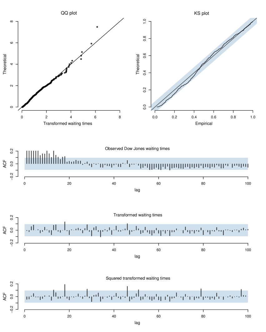
Figure 2: Misspecification analysis for the DJI data. The top left panel shows a QQ-plot of the time transformed waiting times $\hat{v}_{i}=\Lambda(t_{i},t_{i-1};\hat{\theta})$ against a unit exponential distribution. The top right panel shows the corresponding KS plot with 95% confidence band in shaded blue. The three lower panels show the autocorrelations for the observed waiting times, the time transformed waiting times $\hat{v}_{i}$ and $\hat{v}_{i}^{2}$ with 95% confidence band in shaded blue.

To analyze the data, we consider a Hawkes model with intensity reparameterized as

$$\lambda(t;\theta)=\mu+a\sum_{t_{i}<t}\gamma(t-t_{i};\theta)$$ (8.1)

where $a$ is the branching ratio and $\gamma$ is the (exponential) kernel; that is, $\gamma(t;\theta)=\beta\exp(-\beta t)$, see also (2.4) and Section 7. With parameter vector $\theta=(\mu,a,\beta)^{\prime}$, the MLE $\hat{\theta}$ is obtained by maximizing the log-likelihood in (2.9) subject to $\mu,\beta>0$, $0<a<1$ and with initial values from Embrechts et al. (2011). Estimation results are reported in Table 5; the estimated intensity is portrayed in the bottom panel of Figure 1. The MLE $\hat{\theta}$ is very similar to Embrechts et al. (2011), and we observe in particular that the branching ratio $a$ appears to be well inside the stationary region.

As previously emphasized, if the model is correctly specified, the transformed waiting times should be i.i.d. $\mathcal{E}\left(1\right)$. Therefore, the model fit can be evaluated by considering the estimated transformed waiting times

$$\hat{v}_{i}=\Lambda(t_{i},t_{i-1};\hat{\theta}),\quad i=1,2,...,n_{T},$$

with $\Lambda$ defined in (3.2). Figure 2 contains QQ-plots and Kolmogorov-Smirnov (KS) plots, as well as sample autocorrelograms and related tests. Based on these, we see no clear signs of model misspecification. Precisely, the QQ plot of $\hat{v}_{i}$ against a unit exponential distribution has no significant deviations from the identity line, except a few quantiles in the extreme upper tail, as also confirmed by the KS statistic p-value ($0.147$). Moreover, while the observed waiting times $w_{i}$ are autocorrelated, this is not the case for the transformed waiting times $\hat{v}_{i}$ (and its squares, $\hat{v}_{i}^{2}$).

We next compare the different bootstrap algorithms in terms of confidence intervals for the parameters, and compare these with the asymptotic CIs. With $\{\hat{\theta}_{T,i:b}^{\ast}\}_{b=1}^{B}$ the i.i.d. bootstrap realizations of the $i$-th element of $\hat{\theta}_{T}^{\ast}$, the bootstrap CIs reported are based on the empirical $\alpha/2$ and $1-\alpha/2$ quantiles of the empirical distribution function of the $\hat{\theta}_{T,i:b}^{\ast}$’s. In Table 5, while we find no noticeable difference between the parametric and non-parametric bootstraps, the bootstrapped CIs based on the FIB are less wide when compared to the asymptotic and RIB CIs (recall also from the Monte Carlo results that in general the bootstrap coverage probabilities are better than those associated to the asymptotic CIs). The observed difference between the FIB and RIB CIs is likely to be caused by the added randomness in the sequential computation of the RIB. Interestingly, the FIB and RIB bootstrap CIs are further away from the non-stationary region ($a\geq 1$) than the asymptotic CIs.

Table 5: Estimated parameters and bootstrap $95\%$ confidence intervals for DJI data.

	$\hat{\theta}$	Asymptotic	PRFB	NPFB	PRRB	NPRB
$\mu$	0.205	[0.10; 0.31]	[0.19; 0.34]	[0.19; 0.34]	[0.11; 0.38]	[0.13; 0.40]
$a$	0.800	[0.67; 0.93]	[0.67; 0.82]	[0.67; 0.82]	[0.58; 0.91]	[0.54; 0.89]
$\beta$	0.275	[0.15; 0.40]	[0.14; 0.35]	[0.14; 0.30]	[0.18; 0.43]	[0.18; 0.42]

Note: PRFB, NPFB, PRRB, and NPRB refer to parametric fixed intensity, non-parametric fixed intensity, parametric recursive intensity and non-parametric recursive intensity bootstraps.

8.2 COVID-19 Tweets

Figure 3: Danish COVID-19 tweets data. The top panel shows the observed counts at times $\{t_{i}\}$, while the bottom panel shows the the number of events every $15$ minutes. The time resolution for the bottom panel is 15 minute intervals. The vertical dashed line shows the time of the press briefing.

We consider the arrival times of tweets related to the COVID-19 pandemic, recorded on March 11 (06:00-00:00) 2020, when during a press briefing the Danish Prime Minister at 20:30 announced the first lockdown of Denmark. In total, there are $n_{T}=1822$ events from $1166$ unique individuals, with each event time $\{t_{i}\}_{i=0}^{n_{T}}$ ($t_{0}=0$) measured with a time resolution of $1$ second within the $T=18$ hours considered. In order to analyze the effects of the announcement, we analyze the full sample, as well as the pre-press briefing sample (06:00–20:30), and the post-press briefing sample (20:30–00:00). In Figure 3, we show the observed counting process $N(t)$ for $t\in[0,T]$ as well as an initial proxy for the intensity given by the number of events per $15$-minute intervals. It is worth noticing that there is a surge in activity after 20:30, visible both in the counting process and the increased intensity.

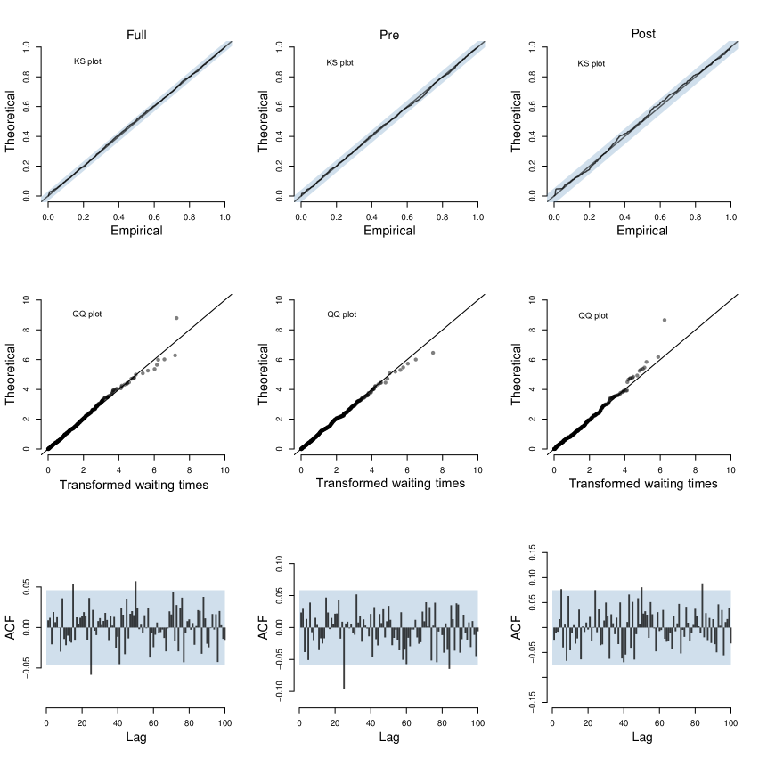
Figure 4: Danish COVID-19 tweets data. The “Full”, “Pre” and “Post” refer to the full sample and the samples pre- and post-announcement on March 11, 2021. The top row presents KS plots for these three time periods. The middle row presents QQ plots for these three time periods. The bottom row presents autocorrelations of the time transformed waiting times for these three periods.

As for the DJI data, we consider the Hawkes model with exponential kernel. Based on the diagnostics (see Figure 4), the model seems to be well specified in all the three (sub)samples. However, we observe a large difference between the estimates reported for the first subsample and for the second subsample, see Table 6. In particular, the effect of the response to the announcement is a substantial increase in the intensity. One may also note that the estimated memory parameter $\beta$ for the full period is between the estimates for the pre-announcement and post-announcement periods. Table 6 also reports asymptotic CIs and FIB CIs. As can clearly be seen, the bootstrap CIs indicates the presence of non-overlapping parameter estimates for the samples before and after the announcement. This possibly reflects different types of dynamics in the two samples, and indicates a structural break around the press briefing. We note that this is not detectable by the standard misspecification tests for the full sample, and is much less pronounced from the reported asymptotic CIs for the three samples (in particular so for the baseline $\mu$).

Table 6: Estimated parameters, asymptotic and bootstrap $95\%$ confidence intervals for Twitter data.

Asymptotic confidence intervals
	Full		Pre		Post
	$\hat{\theta}$	CI	$\hat{\theta}$	CI	$\hat{\theta}$	CI
$\mu$	12.19	[6.85; 21.70]	14.51	[7.64; 27.58]	47.09	[24.76; 89.56]
$a$	0.88	[0.78; 0.94]	0.82	[0.66; 0.92]	0.76	[0.57; 0.89]
$\beta$	8.11	[6.11; 10.78]	5.53	[3.62; 8.43]	21.06	[10.89; 40.74]

Bootstrap confidence intervals
	Full		Pre		Post
	$\hat{\theta}$	CI	$\hat{\theta}$	CI	$\hat{\theta}$	CI
$\mu$	12.21	[11.76; 17.02]	14.54	[13.58; 23.65]	47.07	[44.11; 89.24]
$a$	0.88	[0.84; 0.89]	0.82	[0.71; 0.84]	0.76	[0.55; 0.78]
$\beta$	8.12	[5.71; 9.31]	5.53	[2.64; 6.37]	21.07	[10.42; 41.11]

Note: Non-parametric fixed intensity bootstrap is implemented; ‘Full’, ‘Pre’ and ‘Post’ refer to the full sample and the samples pre- and post-announcement on March 11, 2021.

In addition, we have also considered the power law kernel, where $\gamma(t;\theta)$ in (8.1) is replaced by a power law, see (2.5). Interestingly, unreported results show that, in terms of model misspecification, one is unable to discriminate between the two models, and moreover that the estimates of the baseline $\mu$ and branching ratio $a$ are virtually indistinguishable from those obtained using the exponential kernel. Finally, estimation based on the power law kernel (unlike the exponential kernel) is highly sensitive to initial values, which may reflect the large correlation of the parameter estimators for power law kernels.

9 Conclusions

In this paper we have discussed the theoretical foundations and practical implementations of bootstrap inference for self-exciting point process models. Applications of the bootstrap in order to improve upon the poor quality of asymptotic approximations are scarce in the literature. Classic ‘recursive intensity bootstrap’ (RIB) schemes have been proposed in the recent literature, although without proof of their first-order validity. RIB schemes can also be quite involved to implement in practice, as they generally require numerical integration for the recursive computation of the intensity for each bootstrap repetition. To improve, we have introduced a new bootstrap scheme, the ‘fixed intensity bootstrap’ (FIB), where the conditional intensity is kept fixed across bootstrap repetitions. By doing so, conditionally on the original data the bootstrap data generating process follows a simple inhomogeneous point process with known intensity; therefore, it is very simple to implement and to use in practice. For both bootstrap schemes, we have provided a new bootstrap (asymptotic) theory, which allows to assess bootstrap validity for both bootstraps. Monte Carlo evidence supports the idea that the bootstrap is a valid inference method when applied to point process models.

The results in the paper could be extended in several directions. On top of the obvious extension to multivariate point process models, an interesting one is how to deal with marked point process models. Marked (self-exciting) processes are particularly useful in applications, as the intensity function can be made dependent on a set of ‘marks’ associated to past events (for financial returns, the trading volumes; for energy prices, the magnitude of price spikes; for tweets, the number of followers; for earthquakes modelling, the magnitude of the earthquakes). In this context the proposed FIB seems very powerful as re-sampling with a fixed intensity, even as a function of marks, is feasible and easy to implement. As an example, consider briefly an extension of the Hawkes model with exponential kernel in (2.4). One may include real-valued marks, or covariates, $y_{t}\in\mathbb{R}^{d}$ in the conditional intensity $\lambda(t;\theta)$ as for example,

$$\lambda\left(t;\theta\right)=\mu\left(y_{t}\right)+\alpha\sum_{t_{i}<t}\beta\left(y_{t_{i}}\right)\gamma\left(t-t_{i}\right),$$

where $\mu,\beta:\mathbb{R}^{d}\mathbb{\rightarrow R}_{+}$, see e.g. Clements et al. (2015) for an application to price spikes in electricity markets. Under the assumption of ‘strongly exogenous’ (or, ancillary) marks, similar to exogenous covariates in discrete time Poisson autoregressions (see Agosto et al., 2016) and with $\theta$ the parameters parameterizing the extended Hawkes intensity, estimation and inference based on the FIB utilize the original event times and marks, $\{t_{i},y_{t_{i}}\}_{i=1}^{N(T)}$. Thus, in contrast to the RIB and other existing recursive bootstraps, bootstrap inference based on FIB would not require further assumptions (apart from stationarity) of the covariates.

A further extension is to develop model misspecification-robust bootstrap methods. In particular, throughout the paper we have assumed that the model is correctly specified. This assumption implies that the bootstrap can be implemented parametrically by constructing bootstrap waiting times from an i.i.d. sequence of mean one exponential random variables (the waiting times in transformed time scale), as discussed in Sections 3.2 and 3.3. However, misspecification of the model (in the simplest case, data are modelled as a Poisson process, but the waiting times form a renewal process) may result in i.i.d., but non-exponential (transformed) waiting times. Although in this case the parametric bootstraps could fail, we believe that the non-parametric bootstrap algorithms discussed in Section 5 could serve as the basis of novel misspecification-robust bootstrap methods. All these extensions are left for future research.

Appendix

The appendix contains proofs and results for the bootstrap theory for the FIB and RIB schemes. It is structured as follows. Section A contains a general bootstrap theory to establish asymptotic properties of the bootstrap estimators, as well as central limit theorem (CLT) for inhomogeneous Poisson processes. Section B contains the proofs of Lemma 1 and Theorem 3 for the FIB validity. Similarly, Section C contains the proofs of Lemma 2 and Theorem 4 for the RIB. Some auxiliary lemmas for derivatives of the (bootstrap) likelihood are given in Section D. Finally, Section E contains the proof of the two lemmas in Section A.

Appendix A Auxiliary results

A.1 General asymptotic theory for bootstrap estimators

Before formulating the assumptions for Lemma A.1, we need to properly define a neighborhood $N(\theta)$ of $\theta$ where $\theta\in\operatorname*{int}\Theta$. Without loss of generality, let $\theta=(\theta_{1},...,\theta_{d})^{\prime}\in\Theta\subseteq\mathbb{R}^{d}$, and assume that $\Theta$ is a product of intervals $I_{i}$, $i=1,...,d$, which can be (sub-intervals of) $\mathbb{R},\mathbb{R}_{+}$ or $\mathbb{R}^{+}$. That is, $\Theta=I_{1}\times...\times I_{d}$, and define $N(\theta)$ as

$$N(\theta)=[\theta_{1L},\ \theta_{1U}]\times...\times[\theta_{mL},\ \theta_{mU}],$$ (A.1)

where $\theta_{iL}<\theta_{i}<\theta_{iU}$ for $i=1,2,...,d$. We make the following assumption.

Assumption A.1 Consider a bootstrap log-likelihood, or criterion function $\ell_{T}^{\ast}(\theta)$, which is a function of the bootstrap sample and the parameter $\theta\in\Theta\subseteq\mathbb{R}^{d}$. Assume that $\ell_{T}^{\ast}(\theta)$ is thrice continuously differentiable in $\theta$, and moreover that for the bootstrap true value $\theta_{T}^{\ast}$ it holds that:

(i) $\theta_{T}^{\ast}\rightarrow_{p}\theta_{\dagger}$, where $\theta_{\dagger}\in\operatorname*{int}\Theta$;

(ii) $T^{-1/2}\partial\ell_{T}^{\ast}(\theta_{T}^{\ast})/\partial\theta\overset{d^{\ast}}{\rightarrow}_{p}\mathcal{N(}0,\Omega_{S}),\ \Omega_{S}>0$;

(iii) $-T^{-1}\partial^{2}\ell_{T}^{\ast}(\theta_{T}^{\ast})/\partial\theta\partial\theta^{\prime}\overset{p^{\ast}}{\rightarrow}_{p}\Omega_{I}>0$;

(iv) with $\mathcal{N(}\theta_{\dagger})$ a neighborhood of $\theta_{\dagger}$, see (A.1),

$$\max_{h,i,j=1,...,d}\sup_{\theta\in\mathcal{N(}\theta_{\dagger})}\left|\frac{1}{T}\frac{\partial^{3}\ell_{T}^{\ast}(\theta)}{\partial\theta_{h}\partial\theta_{i}\partial\theta_{j}}\right|\leq c_{T}^{\ast},$$

where $c_{T}^{\ast}\overset{p^{\ast}}{\rightarrow}_{p}c$, $0<c<\infty$.

Lemma A.1

Assume that Assumption A.1 holds. Then in a fixed open neighborhood $U(\theta_{\dagger})$ of $\theta_{\dagger}$ the following holds as $T\rightarrow\infty$:

(i) The probability, conditionally on the original data, that there exists a unique maximum point $\hat{\theta}_{T}^{\ast}$ of $\partial\ell_{T}^{\ast}(\theta)$ which solves the estimating equation $\partial\ell_{T}(\hat{\theta}_{T}^{\ast})/\partial\theta=0$, converges in probability to one;

(ii) $\hat{\theta}_{T}^{\ast}-\theta_{T}^{\ast}\overset{p^{\ast}}{\rightarrow}_{p}0$;

(iii) $T^{1/2}(\hat{\theta}_{T}^{\ast}-\theta_{T}^{\ast})\overset{d^{\ast}}{\rightarrow}_{p}\mathcal{N(}0,\Omega_{I}^{-1}\Omega_{S}\Omega_{I}^{-1})$.

The proof of Lemma A.1 is given in Section E.

Remark A.1

$\overset{}{\text{ }}$

(i) Note that for the restricted bootstrap for testing the simple null hypothesis $\theta=\bar{\theta}$, Assumption A.1(i) is trivially satisfied with $\theta_{\dagger}=\bar{\theta}$. In the general case, $\theta_{T}^{\ast}=\tilde{\theta}_{T}$, where $\tilde{\theta}_{T}$ is an estimator, restricted by the null hypothesis, obtained on the original data; then, Assumption A.1(i) is implied by establishing $\tilde{\theta}_{T}\rightarrow_{p}\theta_{\dagger}$, where under the null $\theta_{\dagger}=\theta_{0}$ while under the alternative, $\theta_{\dagger}$ is a pseudo-true value. For the unrestricted bootstrap, $\theta_{T}^{\ast}=\hat{\theta}_{T}$, and Assumption A.1(i) is implied by establishing the classic consistency result, $\hat{\theta}_{T}\rightarrow_{p}\theta_{0}$.

(ii) As for the condition (iv) in Assumption A.1 on the third derivative of $\ell_{T}^{*}(\theta)$, this may be replaced by a uniform requirement for the second order derivative of $\ell_{T}^{\ast}(\theta)$, $\partial^{2}\ell_{T}^{\ast}(\theta)/\partial\theta\partial\theta^{\prime}$. Specifically, Lemma A.1 holds with condition (iv) in Assumption A.1 replaced by the following condition:

($\text{iv}^{\ast}$) Assume that there exists a continuous function, $f:\mathbb{R}^{d}\rightarrow\mathbb{R}^{d\times d}$ such that,

$$\|T^{-1}\partial^{2}\ell_{T}^{\ast}(\theta)/\partial\theta\partial\theta^{\prime}-f(\theta)\|\overset{p^{\ast}}{\rightarrow}_{p}0$$

uniformly over $\theta\in\mathcal{N(}\theta_{\dagger})$;

see Lange et al. (2011, proof of Lemma A.1) for its non-bootstrap equivalent. $\square$

A.2 Central limit theory for bootstrap point processes

The following lemma is a bootstrap extension of Lemma 2 in Ogata (1978). In Section 4, we consider a bootstrap point process $N^{\ast}(t)$ whose conditional intensity, say $\lambda(t)$, depends only on the original data. Consider an integral of the form

$$Y_{T}^{\ast}:=\int_{0}^{T}\xi_{T}(u)dM^{\ast}(u)$$ (A.2)

where $\xi(u)$ is a function of the original data. We have the following CLT.

Lemma A.2

For all $T\geq 0$, let $N^{\ast}(t)$ be a bootstrap inhomogeneous Poisson process with conditional intensity $\lambda_{T}(t)$ and let $\xi_{T}(t)$ be an $d$-dimensional stochastic process, where both $\lambda_{T}(t)$ and $\xi_{T}(t)$ depend only on the original data. Consider $Y_{T}^{\ast}$ defined in (A.2) with $M^{\ast}(t):=N^{\ast}(t)-\Lambda_{T}(t)$, where $\Lambda_{T}(t)=\int_{0}^{t}\lambda_{T}(u)du$. Then, with $h_{T}(t):=\xi_{T}(t)\xi_{T}(t)^{\prime}\lambda_{T}(t)$, assume that,

$$\frac{1}{T}\int_{0}^{T}h_{T}(t)dt \rightarrow_{p}V<\infty,$$ (A.3)

$$\frac{1}{T}\int_{0}^{T}\|h_{T}(t)\|^{1+\eta}dt =O_{p}(1),$$ (A.4)

for some $\eta>0$. Then if either (i) $\lambda_{T}\left(t\right)\geq\lambda_{L}>0$, or (ii) $\left\|\xi_{T}\left(t\right)\right\|\leq c_{\xi}<\infty$, it holds that

$$T^{-1/2}Y_{T}^{\ast}\overset{d^{\ast}}{\rightarrow}_{p}\mathcal{N}(0,V).$$

The proof of Lemma A.2 is given in Section E.

Appendix B Proofs for the fixed-intensity bootstrap

B.1 Proof of Lemma 1

We first consider the score at the true value, $S_{T}^{\ast}(\theta_{T}^{\ast})=\int_{0}^{T}\hat{\xi}(t)dM^{\ast}(t)$, see (4.3). Conditionally on the data, $M^{\ast}(t)$ is a $\mathcal{F}_{t}^{\ast}$-martingale and $\hat{\xi}(t)$ is a predictable process. Therefore, $\hat{Y}(t):=\int_{0}^{t}\hat{\xi}(s)dM^{\ast}(s)$, as a martingale transformation, is also a $\mathcal{F}_{t}^{\ast}$-martingale (under bootstrap probability) starting from $\hat{Y}(0)=0$. We apply Lemma A.2 to show that $S_{T}^{\ast}(\theta_{T}^{\ast})=\hat{Y}(T)$ satisfies the CLT.

We first verify condition A.3, with $h(t)$ replaced by $\hat{h}(t)=\hat{\xi}(t)\hat{\xi}(t)^{\prime}\hat{\lambda}(t)$ and $V=I(\theta_{0})$. To do so, write $\int_{0}^{T}\hat{h}(t)dt$ as

$$\int_{0}^{T}\hat{h}(t)dt=V_{1,T}+V_{2,T},$$

where $V_{1,T}=T^{-1}\int_{0}^{T}h(t)dt$ and $V_{2,T}=T^{-1}\int_{0}^{T}(\hat{h}(t)-h(t))dt$. Under stationarity (Assumption 1(b)), predictability (Assumption 1(c)) and finite variance of $h(t)$ (Assumption 2(b)), by Lemma 2 (eq. (3.3)) in Ogata (1978),

$$V_{1,T}\rightarrow_{p}E(h(t))=I(\theta_{0}).$$ (B.1)

To show that $V_{2,T}\rightarrow_{p}0$, since $h(t,\theta)$ is continuously differentiable in a neighborhood of $\theta_{0}$ (as implied by Assumption 2(a)) and $\theta_{T}^{\ast}-\theta_{0}=o_{p}(1)$, by the delta method, with $A_{ij}$ denoting the $(i,j)$-th entry of a generic matrix $A$,

$$T^{-1}\int_{0}^{T}(\hat{h}_{ij}(t)-h_{ij}(t))dt=\left(T^{-1}\int_{0}^{T}\partial_{\theta_{0}}h_{ij}(t)dt\right)^{\prime}(\theta_{T}^{\ast}-\theta_{0})(1+o_{p}(1))$$

The proof of Lemma 2 in Ogata (1978) implies that the first term on the right-hand side of the previous equation is of $O_{p}(1)$ provided $E(\partial_{\theta_{0}}h_{ij}(t))$ is finite, which is implied by Assumption 2(a),(b).

We next verify (A.4). As $h(t;\theta)$ is continuously differentiable around $\theta_{0}$ and $\eta>0$, by a Taylor expansion around $\theta_{0}$ and using the fact that $\theta_{T}^{\ast}\rightarrow_{p}\theta_{0}$, it trivially holds that $T^{-1}\int_{0}^{T}\|\hat{h}(t)\|^{1+\eta}dt=O_{p}(1)$, provided $E(|\partial_{\theta_{0}}h_{ij}(t)|^{1+\eta})<\infty$, which holds if, additionally, $E((\partial_{\theta_{i}}\lambda(t;\theta))^{3})<\infty$; see Lemma D.1 in Section D.1. Hence, $T^{-1/2}S_{T}^{\ast}(\theta_{T}^{\ast})\overset{d^{\ast}}{\rightarrow}_{p}\mathcal{N(}0,I(\theta_{0}))$ by Lemma  A.2.

Next consider the Hessian at the true value, $H_{T}^{\ast}(\theta_{T}^{\ast})=\int_{0}^{T}\hat{\zeta}(t)dM^{\ast}(t)-\int_{0}^{T}\hat{h}(t)dt$, see (4.4). Taking expectation conditionally on the data, it follows that

$$E^{\ast}(-T^{-1}H_{T}^{\ast}(\theta_{T}^{\ast}))=T^{-1}\int_{0}^{T}\hat{h}(t)dt=V^{\ast}(T^{-1/2}S_{T}^{\ast}(\theta_{T}^{\ast}))\rightarrow_{p}I(\theta_{0}),$$

as shown above. The convergence in (4.6) then follows provided $T^{-1}H_{T}^{\ast}(\theta_{T}^{\ast})-E^{\ast}(T^{-1}H_{T}^{\ast}(\theta_{T}^{\ast}))=o_{p}^{\ast}(1)$, in probability. To see this, notice that

$$T^{-1}H_{T}^{\ast}(\theta_{T}^{\ast})-E^{\ast}(T^{-1}H_{T}^{\ast}(\theta_{T}^{\ast})) =T^{-1}\int_{0}^{T}\hat{\zeta}(t)dM^{\ast}(t)$$

$$=T^{-1}\int_{0}^{T}\zeta(t)dM^{\ast}(t)+o_{p}(1).$$

The last equality is again by delta method, noticing that $\zeta(t,\theta)$ is continuously differentiable in a neighborhood of $\theta_{0}$ (as implied by Assumption 2(a)) and $\theta_{T}^{\ast}-\theta_{0}=o_{p}(1)$. Specifically,

$$T^{-1}\int_{0}^{T}\hat{\zeta}_{ij}(t)dM^{\ast}(t)-T^{-1}\int_{0}^{T}\zeta_{ij}(t)dM^{\ast}(t)$$

$$\hskip 28.45274pt=\left(T^{-1}\int_{0}^{T}\partial_{\theta_{0}}\zeta_{ij}(t)dM^{\ast}(t)\right)^{\prime}((\theta_{T}^{\ast}-\theta_{0})(1+o_{p}(1))=o_{p}(1)$$

by Lemma 2 in Ogata (1978) under the condition that $E(|\partial_{\theta_{0}}\zeta_{ij}(t)|\lambda(t))<\infty$ as implied by Assumption 2(c). The term $T^{-1}\int\zeta_{ij}(t)dM^{\ast}(t)$ has variance

$$V^{\ast}\left(T^{-1}\int_{0}^{T}\zeta_{ij}(t)dM^{\ast}(t)\right)=T^{-2}\int_{0}^{T}\zeta_{ij}^{2}(t)\hat{\lambda}(t)dt$$ (B.2)

$$\hskip 28.45274pt=T^{-2}\int_{0}^{T}\zeta_{ij}^{2}(t)\lambda(t)dt+o_{p}(T^{-1})$$

using continuous differentiability of $\lambda(t;\theta)$ around $\theta_{0}$. By the ergodic theorem, using $E(\zeta_{ij}^{2}(t)\lambda(t))<\infty$, we have that $T^{-1}\int_{0}^{T}\zeta_{ij}^{2}(t)\lambda(t)dt$ converges in probability, and hence the variance in (B.2) is of $o_{p}(1)$. Taken together, these results imply $-T^{-1}H_{T}^{\ast}(\theta_{T}^{\ast})\rightarrow_{p}I(\theta_{0})$.

B.2 Proof of Theorem 3

The theorem follows by a straightforward application of Lemma A.1. Specifically, Assumption A.0 is satisfied with $\theta^{\dagger}=\theta_{0}$ as by Assumption, $\theta_{T}^{\ast}\rightarrow_{p}\theta_{0}$. Assumptions A.1 and A.2 follow from Lemma 1 with $\Omega_{I}=\Omega_{S}=I(\theta_{0})$. Finally, Assumption A.3 follows from Assumption 2(c), which holds conditionally on the original data; this is shown in the Supplement, Lemma D.2.

Appendix C Proofs for the recursive intensity bootstrap

C.1 Proof of Lemma 2

Recall that, conditionally on the original sample, only $N^{\ast}(t)$ and the associated event times $t_{1}^{\ast},...,t_{n_{T}^{\ast}}^{\ast}$ are random. Moreover, conditionally on the original sample, $N^{\ast}(t)$ has conditional intensity given by $\lambda^{\ast}(t;\theta_{T}^{\ast})$, which in contrast to the FIB, is now a stochastic process even upon conditioning on the original data. As a consequence, at the bootstrap true value $\theta_{T}^{\ast}$, and with $\mathcal{F}_{t}^{\ast}$ denoting the filtration associated to $\{N^{\ast}(s),s\leq t\}$, it holds that $E^{\ast}(dN^{\ast}(t)|\mathcal{F}_{t-}^{\ast})=\lambda^{\ast}(t;\theta_{T}^{\ast})dt$. Notice that $N^{\ast}$ as well as the intensity $\lambda^{\ast}$ depend on the original data through $\theta_{T}^{\ast}$ only. Notice, finally, that $P(\theta_{T}^{\ast}\in\Theta_{0})$ can be made arbitrarily close to one by picking $T$ large enough (such that the bootstrap process can be made stationary upon proper choice of the distribution of the initial values).

Consider first the score evaluated at $\theta_{T}^{\ast}$, see (4.9), which we write as

$$S_{T}^{\ast}(\theta_{T}^{\ast})=\int_{0}^{T}\hat{\xi}^{\ast}(t)dM^{\ast}(t),\quad\hat{\xi}^{\ast}(t):=\partial_{\theta}\log\lambda^{\ast}(t;\theta_{T}^{\ast}).$$

By construction $S_{T}^{\ast}(\theta_{T}^{\ast})$ is a martingale difference array. Assuming without loss of generality that $T$ is an integer we can write

$$T^{-1/2}S_{T}^{\ast}(\theta_{T}^{\ast})=T^{-1/2}\sum_{k=1}^{T}\varepsilon_{T,k}^{\ast},\quad\varepsilon_{T,k}^{\ast}:=\int_{k-1}^{k}\hat{\xi}^{\ast}(t)dM^{\ast}(t),$$

where, conditionally on $\mathcal{F}_{k-}^{\ast}$, $E^{\ast}(\varepsilon_{T,k}^{\ast}|\mathcal{F}_{k-}^{\ast})=0$. We show that $T^{-1/2}S_{T}^{\ast}(\theta_{T}^{\ast})$ satisfies the conditions for the CLT for martingale triangular arrays, see e.g. Theorem 3.4.10 in Durret (2019). The unconditional variance is given by

$$\frac{1}{T}\sum_{k=1}^{T}E^{\ast}((\varepsilon_{T,k}^{\ast})^{2}) =\frac{1}{T}\sum_{k=1}^{T}E^{\ast}\left(\left(\int_{k-1}^{k}\hat{\xi}^{\ast}(t)dM^{\ast}(t)\right)^{2}\right)$$

$$=\frac{1}{T}\sum_{k=1}^{T}E^{\ast}\left(\int_{k-1}^{k}\hat{\xi}^{\ast}(t)\hat{\xi}^{\ast}(t)^{\prime}\lambda^{\ast}(t;\theta_{T}^{\ast})dt\right)$$

$$=E^{\ast}\left(\int_{0}^{1}\hat{\xi}^{\ast}(t)\hat{\xi}^{\ast}(t)^{\prime}\lambda^{\ast}(t;\theta_{T}^{\ast})dt\right)$$

$$=E^{\ast}\left(\int_{0}^{1}\hat{h}^{\ast}(t)dt\right)=I(\theta_{T}^{\ast}),$$

where the last two equalities hold as, with probability tending to one, $\theta_{T}^{\ast}\in\Theta_{0}$. Moreover, by condition (4.11) and for $T$ large enough, $I(\theta_{T}^{\ast})=E(h(t,\theta_{T}^{\ast}))\overset{p}{\rightarrow}E(h(t,\theta_{0}))=:I(\theta_{0})$. To prove that the Lindeberg condition holds in probability, notice that

$$\frac{1}{T}\sum_{k=1}^{T}E^{\ast}\left(\|\varepsilon_{T,k}^{\ast}\|^{2}\mathbb{I}(\|\varepsilon_{T,k}^{\ast}\|>\delta T^{1/2})\right)=E^{\ast}\left(\|\varepsilon_{T,k}^{\ast}\|^{2}\mathbb{I}(\|\varepsilon_{T,k}^{\ast}\|>\delta T^{1/2})\right)\rightarrow_{p}0$$

as, for all $\lambda\in\mathbb{R}^{d}$,

$$E^{\ast}\left((\lambda^{\prime}\varepsilon_{T,k}^{\ast})^{2}\mathbb{I}(\|\varepsilon_{T,k}^{\ast}\|>\delta T^{1/2})\right) \leq E^{\ast}((\lambda^{\prime}\varepsilon_{T,k}^{\ast})^{2})=\lambda^{\prime}E^{\ast}(\varepsilon_{T,k}^{\ast}\varepsilon_{T,k}^{\ast\prime})\lambda$$

$$\leq cE\sup_{\theta\in\Theta_{0}}\|h(t;\theta)\|<\infty,$$

again by (4.11). Hence, $T^{-1/2}S_{T}^{\ast}(\theta_{T}^{\ast})\overset{d^{\ast}}{\rightarrow}\mathcal{N(}0,I(\theta_{0}))$, in probability.

Consider now the Hessian at the true value, given in eq. (4.10). It holds that for $T$ large enough

$$|T^{-1}H_{T}^{\ast}(\theta_{T}^{\ast})-T^{-1}H_{T}^{\ast}(\theta_{0})|\leq\sup_{\theta\in\mathcal{N(}\theta_{0})}|T^{-1}H_{T}^{\ast}(\theta)-T^{-1}H_{T}^{\ast}(\theta_{0})|=o_{p}^{\ast}(1),$$

in probability, where the last equality is found as in the proof of Theorem 3 in Ogata (1978). As $T^{-1}H_{T}^{\ast}(\theta_{0})\overset{p^{\ast}}{\rightarrow}I(\theta_{0})$, the proof is completed.

C.2 Proof of Theorem 4

As for Theorem 3, we apply Lemma A.1 where Assumption A.0 is satisfied with $\theta^{{\dagger}}=\theta_{0}$ and Assumptions A.1 and A.2 follow from Lemma 2 with $\Omega_{I}=\Omega_{S}=I(\theta_{0})$. Finally, Assumption A.3 is verified in Lemma D.3 in Section D.3.

Appendix D Auxiliary lemmas

D.1 Derivative of $h(\cdot)$

Lemma D.1

Consider $h(\cdot)$ defined in Assumption 2(b). Under Assumptions 1 and 2, a sufficient condition for $E(|\partial_{\theta_{0}}h_{ij}(t)|^{1+\eta})<\infty$ is that $E((\partial_{\theta_{i}}\lambda(t;\theta))^{3})<\infty$.

Proof. Without loss of generality we consider the scalar case, $\theta\in\mathbb{R}$. To simplify notation, $h(\theta)$ and $\lambda(\theta)$ are denoted by $h$ and $\lambda$, respectively. Consider

$$\partial_{\theta}h^{1+\eta}=(1+\eta)h^{\eta}\partial_{\theta}h.$$

As

$$|\partial_{\theta}h|=\left|\frac{\left(\partial_{\theta}\lambda\right)\left(\partial_{\theta}^{2}\lambda\right)}{\lambda}-\frac{\left(\partial_{\theta}\lambda\right)^{3}}{\lambda^{2}}\right|\leq\left|\frac{\left(\partial_{\theta}\lambda\right)}{\lambda^{1/2}}\frac{1}{\lambda^{1/2}}\left(\partial_{\theta}^{2}\lambda\right)\right|+\left|\frac{\left(\partial_{\theta}\lambda\right)^{3}}{\lambda^{2}}\right|,$$

we have the inequality

$$|h^{\eta}\partial_{\theta}h|\leq\left|h^{\eta}\frac{\left(\partial_{\theta}\lambda\right)}{\lambda^{1/2}}\frac{1}{\lambda_{L}^{1/2}}\left(\partial_{\theta}^{2}\lambda\right)\right|+\left|h^{\eta}\frac{\left(\partial_{\theta}\lambda\right)^{3}}{\lambda^{2}}\right|:=a_{1}+a_{2},$$

with $a_{1},a_{2}$ implicitly defined. By the Cauchy-Schwartz inequality

$$(E(a_{1}))^{2} \leq E\left(\left(h^{\eta}\left(\frac{1}{\lambda^{1/2}}\partial_{\theta}\lambda\right)\right)^{2}\right)E\left(\left(\partial_{\theta}^{2}\lambda\right)^{2}\right)$$

$$=E\left(h^{2\eta}\frac{1}{\lambda}\left(\partial_{\theta}\lambda\right)^{2}\right)E(\left(\partial_{\theta}^{2}\lambda\right)^{2})=E(h^{1+2\eta})E(\left(\partial_{\theta}^{2}\lambda\right)^{2})<\infty$$

as, by choosing $\eta\leq\frac{1}{2}$, $E(h^{1+2\eta})<\infty$ (by Assumption 2(b), $h$ has finite variance), and $E\left((\partial_{\theta}^{2}\lambda)^{2}\right)<\infty$ (by Assumption 2(a)). Consider now $a_{2}$. Since

$$h^{\eta}\frac{\left(\partial_{\theta}\lambda\right)^{3}}{\lambda^{2}}=h^{\eta}\frac{\left(\partial_{\theta}\lambda\right)^{3/2}}{\lambda^{3/4}}\frac{\left(\partial_{\theta}\lambda\right)^{3/2}}{\lambda^{5/4}}=h^{\frac{3}{4}+\eta}\frac{\left(\partial_{\theta}\lambda\right)^{3/2}}{\lambda^{5/4}},$$

we can consider the inequality

$$E(a_{2})\leq\frac{1}{\lambda_{L}^{5/4}}E\left|h^{\frac{3}{4}+\eta}\left(\partial_{\theta}\lambda\right)^{3/2}\right|$$

which, by the Cauchy-Schwartz inequality, is bounded provided $E\left((h^{\frac{3}{4}+\eta})^{2}\right)=E(h^{\frac{3}{2}+2\eta})<\infty$ and $E\left((\partial_{\theta}\lambda)^{3}\right)<\infty$. The former inequality holds by the finite variance assumption on $h$ by choosing $\eta<1/4$, while the latter holds by assumption.

D.2 Third derivative of the FIB likelihood

Lemma D.2

Under the conditions of Theorem 3 for the FIB,

$$\sup_{\theta\in N_{\epsilon}\left(\theta_{{\dagger}}\right)}|\partial_{\theta_{i},\theta_{j},\theta_{k}}^{3}\tfrac{1}{T}l_{T}^{\ast}\left(t;\theta\right)|\leq c_{T}^{\ast}\overset{p^{\ast}}{\rightarrow}_{p}c.$$

Proof. Without loss of generality, to simplify notation we assume that $\theta$ is scalar. It follows that

$$\sup_{\theta\in\mathcal{N(}\theta_{0})}\left|\frac{1}{T}\partial_{\theta}^{3}l_{T}^{\ast}\left(\theta\right)\right| =\sup_{\theta\in\mathcal{N(}\theta_{0})}\left|\frac{1}{T}\int_{0}^{T}\partial_{\theta}^{3}\log\lambda(t,\theta)dN^{\ast}(t)-\frac{1}{T}\int_{0}^{T}\partial_{\theta}^{3}\lambda(t,\theta)dt\right|$$

$$\leq\sup_{\theta\in\mathcal{N(}\theta_{0})}\left|\frac{1}{T}\int_{0}^{T}\partial_{\theta}^{3}\log\lambda(t,\theta)dN^{\ast}(t)\right|$$

$$+\sup_{\theta\in\mathcal{N(}\theta_{0})}\left|\frac{1}{T}\int_{0}^{T}\partial_{\theta}^{3}\lambda(t,\theta)dt\right|=:A_{T}^{\ast}+B_{T}$$

where

$$B_{T}:=\sup_{\theta\in\mathcal{N(}\theta_{0})}\left|\frac{1}{T}\int_{0}^{T}\partial_{\theta}^{3}\lambda(t,\theta)dt\right| \leq\frac{1}{T}\int_{0}^{T}c(t)dt\rightarrow_{p}E(c(t))$$

$$A_{T}^{\ast}:=\sup_{\theta\in\mathcal{N(}\theta_{0})}\left|\frac{1}{T}\int_{0}^{T}\partial_{\theta}^{3}\log\lambda(t,\theta)dN^{\ast}(t)\right| \leq\frac{1}{T}\int_{0}^{T}d(t)dN^{\ast}(t)\overset{p^{\ast}}{\rightarrow}_{p}E(d(t)\lambda(t)).$$

The first convergence follows from the LLN for stationary and ergodic processes. To see the second convergence, consider the following decomposition:

$$\frac{1}{T}\int_{0}^{T}d(t)dN^{\ast}(t)=\frac{1}{T}\int_{0}^{T}d(t)dM^{\ast}(t)+\frac{1}{T}\int_{0}^{T}d(t)\hat{\lambda}(t)dt$$ (D.1)

where $T^{-1}\int_{0}^{T}d(t)dM^{\ast}(t)=O_{p}^{\ast}(T^{-1/2})$, in probability. By a Taylor expansion,

$$\frac{1}{T}\int_{0}^{T}d(t)\hat{\lambda}(t)dt=\frac{1}{T}\int_{0}^{T}d(t)\lambda(t)dt+\frac{1}{T}\int_{0}^{T}d(t)\partial_{\theta}\lambda(t)dt(\theta_{T}^{\ast}-\theta_{0})(1+o_{p}(1))$$

where

$$\frac{1}{T}\int_{0}^{T}d(t)\lambda(t)dt\rightarrow_{p}E(d(t)\lambda(t))<\infty$$

by Assumption 2(c). To see that the last term on the right hand side is negligible, it suffices no show that

$$E|d(t)\partial_{\theta}\lambda(t)|<\infty,$$

which holds as

$$E|d(t)\partial_{\theta}\lambda(t)|=E\left|\left(\lambda(t)d(t)\right)\left(\frac{\partial_{\theta}\lambda(t)}{\lambda(t)}\right)\right|<\infty$$

by the Cauchy-Schwarz inequality, as $E\left((\lambda(t)d(t))^{2}\right)<\infty$ and $E((\frac{\partial_{\theta}\lambda(t)}{\lambda(t)})^{2})<(\lambda_{L})^{-1}E(\partial_{\theta}\lambda(t))^{2}<\infty$. For the first term in (D.1), we have (see also the proof of Lemma 1)

$$V^{\ast}\left(\frac{1}{T}\int_{0}^{T}d(t)dM^{\ast}(t)\right) =\frac{1}{T^{2}}\int_{0}^{T}d(t)^{2}\hat{\lambda}(t)dt=\frac{1}{T^{2}}\int_{0}^{T}d(t)^{2}\lambda(t)dt$$

$$+\frac{1}{T^{2}}\int_{0}^{T}d(t)^{2}\partial_{\theta}\lambda(t)dt\left((\hat{\theta}-\theta_{0})(1+o_{p}(1))\right)$$

$$=O_{p}(T^{-1})$$

as $\int_{0}^{T}d(t)^{2}\lambda(t)dt\leq\lambda_{L}^{-1}\int_{0}^{T}d(t)^{2}\lambda^{2}(t)dt=O_{p}(T)$, and

$$\frac{1}{T^{2}}\int_{0}^{T}d(t)^{2}\partial_{\theta}\lambda(t)dt\leq\frac{1}{T}\sup_{t\in[0,T]}|d(t)\lambda(t)|\frac{1}{T\lambda_{L}}\int_{0}^{T}d(t)|\partial_{\theta}\lambda(t)|dt$$

where for any $\varepsilon>0$,

$$P\left(\frac{1}{T}\sup_{t\in[0,T]}|d(t)\lambda(t)|>\varepsilon\right) =\int_{0}^{T}\left(P(|d(t)\lambda(t)|>\varepsilon T\right)dt$$

$$\leq T\frac{E|d(t)\lambda(t)|^{2}}{\varepsilon^{2}T^{2}}=O_{p}(T^{-1})$$

under the stated conditions and $T^{-1}\int_{0}^{T}d(t)|\partial_{\theta}\lambda(t)|dt=O_{p}(1)$ as shown above.

D.3 Third derivative of the RIB likelihood

Lemma D.3

Under the conditions of Theorem 4 for the RIB,

$$\sup_{\theta\in N_{\epsilon}(\theta_{0})}|\partial_{\theta_{i},\theta_{j},\theta_{k}}^{3}\frac{1}{T}l_{T}^{\ast}(t;\theta)|\leq c_{T}^{\ast}\overset{p^{\ast}}{\rightarrow}_{p}c.$$

Proof. Similarly to the proof of Lemma D.2, we have

$$\sup_{\theta\in\mathcal{N(}\theta_{0})}\left|\frac{1}{T}\partial_{\theta}^{3}l_{T}^{\ast}(\theta)\right| =\sup_{\theta\in\mathcal{N(}\theta_{0})}\left|\frac{1}{T}\int_{0}^{T}\partial_{\theta}^{3}\log\lambda^{\ast}(t,\theta)dN^{\ast}(t)-\frac{1}{T}\int_{0}^{T}\partial_{\theta}^{3}\lambda^{\ast}(t,\theta)dt\right|$$

$$\leq\sup_{\theta\in\mathcal{N(}\theta_{0})}\left|\frac{1}{T}\int_{0}^{T}\partial_{\theta}^{3}\log\lambda^{\ast}(t,\theta)dN^{\ast}(t)\right|$$

$$+\sup_{\theta\in\mathcal{N(}\theta_{0})}\left|\frac{1}{T}\int_{0}^{T}\partial_{\theta}^{3}\lambda^{\ast}(t,\theta)dt\right|=:A_{T}^{\ast}+B_{T}^{\ast}.$$

Notice that, in contrast to the FIB, the term $B_{T}^{\ast}$ now depends on the bootstrap data. The reminder of the proof follows the same lines of the proof of Lemma D.2. The difference is that, since conditionally on the data, the intensity of the bootstrap process is a stochastic process, in order to bound the third order derivatives of $\lambda^{\ast}(t,\theta)$ and $\log\lambda^{\ast}(t,\theta)$, the additional condition in Assumption 2(c^∗) is required.

Appendix E Miscellaneous proofs for bootstrap theory

E.1 Proof of Lemma A.1

The proof is based on the proof of Lemma 1 in Jensen and Rahbek (2004) [henceforth, JR04], which is modified here for the bootstrap. With $\tilde{\ell}_{T}(\theta)=-\frac{2}{T}\ell_{T}^{\ast}(\theta)$, $\partial\tilde{\ell}_{T}(\theta_{T}^{\ast})=\left.\partial\tilde{\ell}_{T}(\theta)\partial\theta^{\prime}\right|_{\theta=\theta_{T}^{\ast}}$ and $\partial^{2}\tilde{\ell}_{T}(\theta^{\ast})=\left.\partial^{2}\tilde{\ell}_{T}(\theta)/\partial\theta\partial\theta^{\prime}\right|_{\theta=\theta_{T}^{\ast}}$, using Assumption A.1(iv) it follows as in JR04 that for any $v_{1},v_{2}\in\mathbb{R}^{d}$, $\theta\in\mathcal{N(}\theta_{\dagger})$ and $T$ large enough, such that $\theta_{T}^{\ast}\in\mathcal{N(}\theta_{\dagger})$ (by Assumption A.1(i)),

$$\left|v_{1}^{\prime}\left(\partial^{2}\tilde{\ell}_{T}(\theta)-\partial^{2}\tilde{\ell}_{T}(\theta_{T}^{\ast})\right)v_{2}\right|\leq\left\|v_{1}\right\|\left\|v_{2}\right\|\left\|\theta-\theta_{T}^{\ast}\right\|\tilde{c}_{T}^{\ast},$$ (E.1)

where $\tilde{c}_{T}^{\ast}=2d^{3/2}c_{T}^{\ast}$. Next, by continuity, $\tilde{\ell}_{T}(\theta)$ attains its minimum in any compact neighborhood $K(\theta_{\dagger},r)=\{\theta|\ \|\theta-\theta_{\dagger}\|\leq r\}\subseteq\mathcal{N(}\theta_{\dagger})$ of $\theta_{\dagger}$. Similar to JR04, we next show that with probability tending to one, in probability, as $T\rightarrow\infty,$ $\tilde{\ell}_{T}(\theta)$ cannot obtain its minimum on the boundary of $K(\theta_{\dagger},r)$ and that $\tilde{\ell}_{T}(\theta)$ is convex in the interior of $K(\theta_{\dagger},r)$, $\operatorname*{int}K(\theta_{\dagger},r)$. Specifically, with $v_{\theta}^{\ast}:=(\theta-\theta_{T}^{\ast}),$ and $\bar{\theta}$ on the line from $\theta$ to $\theta_{T}^{\ast}$, Taylor’s formula gives

$$\tilde{\ell}_{T}(\theta)-\tilde{\ell}_{T}(\theta_{T}^{\ast})=\partial\tilde{\ell}_{T}(\theta_{T}^{\ast})v_{\theta}^{\ast}+\tfrac{1}{2}v_{\theta}^{\ast\prime}\partial^{2}\tilde{\ell}_{T}(\bar{\theta})v_{\theta}^{\ast}=$$ (E.2)

$$\partial\tilde{\ell}_{T}(\theta_{T}^{\ast})v_{\theta}^{\ast}+\tfrac{1}{2}v_{\theta}^{\ast\prime}\left[\tilde{\Omega}_{I}+(\partial^{2}\tilde{\ell}_{T}(\theta_{T}^{\ast})-\tilde{\Omega}_{I})+(\partial^{2}\tilde{\ell}_{T}(\bar{\theta})-\partial^{2}\tilde{\ell}_{T}(\theta_{T}^{\ast}))\right]v_{\theta}^{\ast},$$

where $\tilde{\Omega}_{I}=2\Omega_{I}$. Denote by $\delta_{T}^{\ast}$ and $\rho>0$, the smallest eigenvalues of the matrix $[\partial^{2}\tilde{\ell}_{T}(\theta_{T}^{\ast})-\tilde{\Omega}_{I}]$ and $\tilde{\Omega}_{I}$, respectively, where $\delta_{T}^{\ast}\overset{p^{\ast}}{\rightarrow}_{p}0$ by Assumption A.1(iii) and the fact that the smallest eigenvalue of a $d\times d$ symmetric matrix $M$ is continuous in $M$. Taken together, Assumption A.1(ii) and (iv), with $\tilde{c}=2k^{3/2}c$, and the uniform upper bound in (E.1) imply that

$$\inf_{\theta:\|\theta-\theta_{\dagger}\|=r}[\tilde{\ell}_{T}(\theta)-\tilde{\ell}_{T}(\theta_{T}^{\ast})] \geq-\|\partial\tilde{\ell}_{T}(\theta_{T}^{\ast})\|\left\|v_{\theta}^{\ast}\right\|+\tfrac{1}{2}\left\|v_{\theta}^{\ast}\right\|^{2}\left[\rho+\delta_{T}^{\ast}-\tilde{c}_{T}^{\ast}r\right]$$

$$\overset{p^{\ast}}{\rightarrow}_{p}\tfrac{1}{2}[\rho-\tilde{c}r]r^{2}=:\eta,$$

where we have used $\left\|v_{\theta}^{\ast}\right\|\rightarrow_{p}r=\left\|\theta-\theta_{\dagger}\right\|$ by Assumption A.1(i). Hence, if $r<\rho/\tilde{c}$ then $\inf_{\theta:\|\theta-\theta_{\dagger}\|=r}[\tilde{\ell}_{T}(\theta)-\tilde{\ell}_{T}(\theta_{T}^{\ast})]\geq\eta>0$ with probability tending to one (in probability). As $\tilde{\ell}_{T}(\theta)|_{\theta=\theta_{T}^{\ast}}-\tilde{\ell}_{T}(\theta_{T}^{\ast})=0$, this implies that the probability that $\tilde{\ell}_{T}(\theta)$ attains its minimum on the boundary of $K(\theta_{\dagger},r)$ tends to zero (in probability). Next, for $\theta\in K(\theta_{\dagger},r)$ and $v\in\mathbb{R}^{d}$, rewriting $v^{\prime}\partial^{2}\tilde{\ell}_{T}(\theta)v$ as in (E.2) one finds

$$v^{\prime}\partial^{2}\tilde{\ell}_{T}(\theta)v\geq\|v\|^{2}(\rho+\delta_{T}^{\ast}-r\tilde{c}_{T}^{\ast})\overset{p^{\ast}}{\rightarrow}_{p}\|v\|^{2}(\rho-r\tilde{c}).$$

Hence, if $r<\rho/\tilde{c}$ the probability that, conditionally on the data, $\tilde{\ell}_{T}(\theta)$ is strongly convex in the interior of $K(\theta_{\dagger},r)$ tends to $1$ in probability, and therefore it has at most one stationary point (with probability tending to one). As in JR04, this establishes Part (i) of the lemma with $U(\theta_{\dagger})=\operatorname*{int}K(\theta_{\dagger},r)$: $\hat{\theta}_{T}^{\ast}$ is the unique minimum point of $\tilde{\ell}_{T}(\theta)$ in $U(\theta_{\dagger})$, and $\partial\tilde{\ell}_{T}(\hat{\theta}_{T}^{\ast})=0$ implies $\partial\ell_{T}^{\ast}(\hat{\theta}_{T}^{\ast})=0$. Likewise, it follows that $\hat{\theta}_{T}^{\ast}-\theta_{\dagger}\overset{p^{\ast}}{\rightarrow}_{p}0$, which establishes Part (ii) of the lemma, as by Assumption A.1(i),

$$\left\|\hat{\theta}_{T}^{\ast}-\theta_{T}^{\ast}\right\|\leq\left\|\hat{\theta}_{T}^{\ast}-\theta_{\dagger}\right\|+\left\|\theta_{\dagger}-\theta_{T}^{\ast}\right\|\overset{p^{\ast}}{\rightarrow}_{p}0.$$

As to Part (iii) of the lemma, note that by Assumption A.1(ii) and Taylor’s formula for $\partial\tilde{\ell}_{T}(\theta)/\partial\theta_{j},j=1,\dots,d$,

$$T^{1/2}\partial\tilde{\ell}_{T}(\theta_{T}^{\ast})=(\tilde{\Omega}_{I}+Q_{T}(\bar{\theta}))T^{1/2}(\hat{\theta}_{T}^{\ast}-\theta_{T}^{\ast}),$$ (E.3)

where $Q_{T}(\bar{\theta}):=\partial^{2}\tilde{\ell}_{T}(\bar{\theta})-\tilde{\Omega}_{I}$, $\bar{\theta}$ being a point on the line from $\theta_{T}^{\ast}$ to $\hat{\theta}_{T}^{\ast}$. Next, $Q_{T}(\bar{\theta})\overset{p^{\ast}}{\rightarrow}_{p}0$ by (E.1),

$$|v_{1}^{\prime}Q_{T}(\bar{\theta})v_{2}| \leq|v_{1}^{\prime}\left(\partial^{2}\tilde{\ell}_{T}(\bar{\theta})-\partial^{2}\tilde{\ell}_{T}(\theta_{T}^{\ast})\right)v_{2}|+|v_{1}^{\prime}(\partial^{2}\tilde{\ell}_{T}(\theta_{T}^{\ast})-\tilde{\Omega}_{I})v_{2}|$$

$$\leq\|v_{1}\|\|v_{2}\|\|\bar{\theta}-\theta_{T}^{\ast}\|\tilde{c}_{T}^{\ast}+|v_{1}^{\prime}(\partial^{2}\tilde{\ell}_{T}(\theta_{T}^{\ast})-\tilde{\Omega}_{I})v_{2}|\overset{p^{\ast}}{\rightarrow}_{p}0$$

since $\bar{\theta}-\theta_{T}^{\ast}\overset{p^{\ast}}{\rightarrow}_{p}0$, $\tilde{c}_{T}^{\ast}\overset{p^{\ast}}{\rightarrow}_{p}\tilde{c}<\infty$ and applying Assumption A.1(iii). Hence, using Assumption A.1(ii), (E.3) gives the desired,

$$T^{1/2}(\hat{\theta}_{T}^{\ast}-\theta_{T}^{\ast})\overset{d^{\ast}}{\rightarrow}_{p}\mathcal{N(}0,\tilde{\Omega}_{I}^{-1}2^{2}\Omega_{S}\tilde{\Omega}_{I}^{-1})=\mathcal{N(}0,\Omega_{I}^{-1}\Omega_{S}\Omega_{I}^{-1}).$$

This completes the proof.

E.2 Proof of Lemma A.2

Assume w.l.g. that $T$ is an integer and let $\varepsilon_{T,k}^{\ast}:=\int_{k-1}^{k}\xi_{T}(t)dM^{\ast}(t)$, such that $Y_{T}^{\ast}=\sum_{k=1}^{T}\varepsilon_{T,k}^{\ast}$. Clearly, $\varepsilon_{T,k}^{\ast}$ defined a martingale difference array [mda] with average conditional variance given by

$$\frac{1}{T}\sum_{k=1}^{T}E^{\ast}((\varepsilon_{T,k}^{\ast})^{2}|\mathcal{F}_{k-}^{\ast})$$

$$=\frac{1}{T}\sum_{k=1}^{T}E^{\ast}\left(\left.\left(\int_{k-1}^{k}\xi_{T}(t)dM^{\ast}(t)\right)\left(\int_{k-1}^{k}\xi_{T}(t)dM^{\ast}(t)\right)^{\prime}\right|\mathcal{F}_{k-}^{\ast}\right)$$

$$=\frac{1}{T}\sum_{k=1}^{T}E^{\ast}\left(\left.\int_{k-1}^{k}\xi_{T}(t)\xi_{T}(t)^{\prime}[dM^{\ast}(t)]^{2}\right|\mathcal{F}_{k-}^{\ast}\right)$$

$$=\frac{1}{T}\sum_{k=1}^{T}E^{\ast}\left(\left.\int_{k-1}^{k}\xi_{T}(t)\xi_{T}(t)^{\prime}E^{\ast}([dM^{\ast}(t)]^{2}|\mathcal{F}_{t-}^{\ast})\right|\mathcal{F}_{k-}^{\ast}\right)$$

$$=\frac{1}{T}\sum_{k=1}^{T}E^{\ast}\left(\left.\int_{k-1}^{k}\xi_{T}(t)\xi_{T}(t)^{\prime}\lambda_{T}(t)dt\right|\mathcal{F}_{k-}^{\ast}\right)$$

$$=\frac{1}{T}\sum_{k=1}^{T}\int_{k-1}^{k}\xi_{T}(t)\xi_{T}(t)^{\prime}\lambda_{T}(t)dt=\frac{1}{T}\int_{0}^{T}h_{T}(t)dt\rightarrow_{p}V$$

by Assumption (A.3). By the CLT for mda’s, see e.g. Corollary 3.1 in Hall and Heyde (1980), $T^{-1/2}Y_{T}^{\ast}\overset{d^{\ast}}{\rightarrow}_{p}\mathcal{N(}0,V)$, provided that the Lindeberg condition holds on $\varepsilon_{T,k}^{\ast}$, which we prove next.

Consider, for some $\eta>0$,

$$L_{T}^{\ast}:=\frac{1}{T}\sum_{k=1}^{T}E^{\ast}(\|\varepsilon_{T,k}^{\ast}\|^{2}\mathbb{I}(\|\varepsilon_{T,k}^{\ast}\|>T^{1/2}\delta)|\mathcal{F}_{k-1}^{\ast}),$$

for which it follows that,

$$L_{T}^{\ast} \leq\frac{1}{T^{1+\eta}\delta^{2\eta}}\sum_{k=1}^{T}E^{\ast}\left(\|\varepsilon_{T,k}^{\ast}\|^{2(1+\eta)}|\right)$$

$$=\frac{1}{T^{\eta}\delta^{2\eta}}\frac{1}{T}\sum_{k=1}^{T}E^{\ast}\left(\left\|\int_{k-1}^{k}\xi_{T}(t)dM^{\ast}(t)\right\|^{2(1+\eta)}\right).$$

Next, by Lemma A.2 in Clinet and Yoshida (2017) with $p=\log_{2}(2(1+\eta))$, it holds (with $c$ a generic constant),

$$E^{\ast}\left(\left\|\int_{k-1}^{k}\xi_{T}(t)dM^{\ast}(t)\right\|^{2(1+\eta)}\right)$$

$$\leq\ cE^{\ast}\left(\int_{k-1}^{k}\left\|\xi_{T}(t)\right\|^{2(1+\eta)}\lambda_{T}(t)dt\right)+cE^{\ast}\left|\int_{k-1}^{k}\|\xi_{T}(t)\|^{2}\lambda_{T}(t)dt\right|^{1+\eta}$$

$$=\ c\int_{k-1}^{k}\|\xi_{T}(t)\|^{2(1+\eta)}\lambda_{T}(t)dt+c\left(\int_{k-1}^{k}\|\xi_{T}(t)\|^{2}\lambda_{T}(t)dt\right)^{1+\eta}$$

$$\leq\ c\int_{k-1}^{k}\|\xi_{T}(t)\|^{2\left(1+\eta\right)}\lambda_{T}(t)dt+c\int_{k-1}^{k}\|\xi_{T}(t)\|^{2(1+\eta)}\lambda_{T}(t)^{1+\eta}dt$$

Consider the second term:

$$\frac{1}{T^{1+\eta}}\sum_{k=1}^{T}\int_{k-1}^{k}\|\xi_{T}(t)\|^{2(1+\eta)}\lambda_{T}(t)^{1+\eta}dt=\frac{1}{T^{1+\eta}}\int_{0}^{T}\|h_{T}(t)\|^{1+\eta}dt=O_{p}\left(T^{-\eta}\right)$$

by finite variance of $h_{T}(t)$. Next, for the first term, assume that $\lambda_{T}(t)\geq\lambda_{L}>0$. Then

$$\frac{1}{T^{1+\eta}}\int_{0}^{T}\|\xi_{T}(t)\|^{2(1+\eta)}\lambda_{T}(t)dt =\frac{1}{T^{1+\eta}}\int_{0}^{T}\|h_{T}(t)\|^{1+\eta}\frac{1}{\lambda_{T}^{\eta}(t)}dt$$

$$\leq\frac{1}{\lambda_{L}^{\eta}T^{1+\eta}}\int_{0}^{T}\|h_{T}(t)\|^{1+\eta}dt=O_{p}\left(T^{-\eta}\right).$$

Finally, assuming instead for the first term $\left\|\xi_{T}\left(t\right)\right\|\leq c_{\xi}<\infty$, it follows that,

$$E\left[\|\xi_{T}(t)\|^{2(1+\eta)}\lambda_{T}(t)\right]\leq c_{\xi}^{2(1+\eta)}E\left(\lambda_{T}^{2}\left(t\right)\right)^{1/2}<\infty,$$

and hence $\int_{0}^{T}\|\xi_{T}(t)\|^{2(1+\eta)}\lambda_{T}(t)dt=O_{p}\left(T\right)$ as desired.

References

- Agosto et al. (2016) Agosto, A., G. Cavaliere, D. Kristensen, and A. Rahbek (2016). Modeling corporate defaults: Poisson autoregressions with exogenous covariates (PARX). Journal of Empirical Finance, 38, 640–663.
- Aït-Sahalia et al. (2015) Aït-Sahalia, Y., J. Cacho-Diaz, and R. J. Laeven (2015). Modeling financial contagion using mutually exciting jump processes. Journal of Financial Economics, 117(3), 585–606.
- Bauwens and Hautsch (2009) Bauwens, L. and N. Hautsch (2009). Modelling financial high frequency data using point processes. In Handbook of Financial Time Series (pp. 953–979). Springer.
- Billingsley (1968) Billingsley, P. (1968). Convergence of Probability Measures. John Wiley & Sons.
- Bowsher (2007) Bowsher, C. G. (2007). Modelling security market events in continuous time: Intensity based, multivariate point process models. Journal of Econometrics, 141(2), 876–912.
- Cavaliere and Georgiev (2020) Cavaliere, G. and I. Georgiev (2020). Inference under random limit bootstrap measures. Econometrica, 80(6), 2547–2574.
- Cavaliere et al. (2015) Cavaliere, G., H. B. Nielsen, and A. Rahbek (2015). Bootstrap testing of hypotheses on co-integration relations in vector autoregressive models, Econometrica, 83, 813–831.
- Cavaliere et al. (2018) Cavaliere, G., R. S. Pedersen, and A. Rahbek (2018). The fixed volatility bootstrap for a class of ARCH() models. Journal of Time Series Analysis, 39(6), 920–941.
- Cavaliere and Rahbek (2021) Cavaliere, G. and A. Rahbek (2021). A primer on bootstrap testing of hypotheses in time series models: with and application to double autoregressive models. Econometric Theory, 37, 2021, 1–48.
- Cavaliere et al. (2012) Cavaliere, G., A. Rahbek, and A. R. Taylor (2012). Bootstrap determination of the co-integration rank in vector autoregressive models. Econometrica, 80(4), 1721–1740.
- Clements et al. (2015) Clements, A. E., R. Herrera, and A. S. Hurn (2015). Modelling interregional links in electricity price spikes. Energy Economics, 51, 383–393.
- Clinet and Yoshida (2017) Clinet, S. and N. Yoshida (2017). Statistical inference for ergodic point processes and application to limit order book. Stochastic Processes and their Applications, 127(6), 1800–1839.
- Cowling et al. (1996) Cowling, A., P. Hall, and M. J. Phillips (1996). Bootstrap confidence regions for the intensity of a Poisson point process. Journal of the American Statistical Association, 91(436), 1516–1524.
- Daley and Vere-Jones (2003) Daley, D. J. and D. Vere-Jones (2003). An Introduction to the Theory of Point Processes: Volume I: Elementary Theory and Methods. Springer.
- Dassios and Zhao (2013) Dassios, A. and H. Zhao. (2013). Exact simulation of Hawkes process with exponentially decaying intensity. Electronic Communications in Probability, 18.
- Dolado and María-Dolores (2002) Dolado, J. J. and R. María-Dolores (2002). Evaluating changes in the Bank of Spain’s interest rate target: an alternative approach using marked point processes, Oxford Bulletin of Economics and Statistics, 64, 159–182.
- Durret (2019) Durret, R. (2019). Probability: Theory and Examples, Fifth edition, Cambridge University Press.
- Embrechts et al. (2011) Embrechts, P., T. Liniger, and L. Lin (2011). Multivariate Hawkes processes: an application to financial data. Journal of Applied Probability, 48(A), 367–378.
- Engle and Russell (1998) Engle, R.F. and J. Russell (1998). Autoregressive Conditional Duration: a new model for irregularly spaced transaction data. Econometrica, 66, 1127–1162.
- Fernandes and Gramming (2005) Fernandes, M. and J. Gramming (2005). Nonparametric specification tests for conditional duration models. Journal of Econometrics, 127, 35–68.
- Gao et al. (2015) Gao, J., N. H. Kim, and P. W. Saart (2015). A misspecification test for multiplicative error models of non-negative time series processes. Journal of Econometrics, 189, 349–359.
- Gonçalves and Kilian (2004) Gonçalves, S. and L. Kilian (2004). Bootstrapping autoregressions with conditional heteroskedasticity of unknown form. Journal of Econometrics, 123(1), 89–120.
- Hall and Heyde (1980) Hall, P. and C. C. Heyde. (1980). Martingale Limit Theory and Its Application. Academic press.
- Hawkes and Oakes (1974) Hawkes, A. G. and D. Oakes (1974). A cluster process representation of a self-exciting process. Journal of Applied Probability, 11(3), 493–503.
- Jensen and Rahbek (2004) Jensen, S. T. and A. Rahbek (2004). Asymptotic inference for nonstationary GARCH. Econometric Theory, 20(6), 1203–1226.
- Lange et al. (2011) Lange, T., A. Rahbek, and S. T. Jensen (2011). Estimation and asymptotic inference in the AR-ARCH model. Econometric Reviews, 30(2), 129–153.
- Lewis and Shedler (1979) Lewis, P. W. and G. S. Shedler (1979). Simulation of nonhomogeneous Poisson processes by thinning. Naval Research Logistics Quarterly, 26(3), 403–413.
- Mohler et al. (2011) Mohler, G. O., M. B. Short, P. J. Brantingham, F. P. Schoenberg, and G. E. Tita (2011). Self-exciting point process modeling of crime. Journal of the American Statistical Association, 106(493), 100–108.
- Ogata (1978) Ogata, Y. (1978). The asymptotic behavior of maximum likelihood estimators for stationary point processes. Annals of the Institute of Statistical Mathematics, 30(2), 243–261.
- Ogata (1981) Ogata, Y. (1981). On Lewis’ simulation method for point processes. IEEE Transactions on Information Theory, 27(1), 23–31.
- Ogata (1988) Ogata, Y. (1988). Statistical models for earthquake occurrences and residual analysis for point processes. Journal of the American Statistical Association, 83(401), 9–27.
- Ozaki (1979) Ozaki, T. (1979). Maximum likelihood estimation of Hawkes’ self-exciting point processes. Annals of the Institute of Statistical Mathematics, 31(1), 145–155.
- Perera et al. (2016) Perera, I., J. Hidalgo, and M. J. Silvapulle (2016). A Goodness-of-fit test for a class of autoregressive conditional duration models. Econometric Reviews, 35(6), 1111–1141.
- Perera and Silvapulle (2017) Perera, I. and M. J. Silvapulle (2017). Specification tests for multiplicative error models. Econometric Theory, 33, 413–438.
- Perera and Silvapulle (2021) Perera, I. and M. J. Silvapulle (2021). Bootstrap based probability forecasting in multiplicative error models. Journal of Econometrics, 221, 1–24.
- Rasmussen (2013) Rasmussen, J. G. (2013). Bayesian inference for Hawkes processes. Methodology and Computing in Applied Probability, 15(3), 623–642.
- Reinhart (2018) Reinhart, A. (2018). A review of self-exciting spatio-temporal point processes and their applications. Statistical Science, 33(3), 299–318.
- Rizoiu et al. (2017) Rizoiu, M. A., Y. Lee, S. Mishra, and L. Xie (2017). A tutorial on Hawkes processes for events in social media. arXiv:1708.06401.
- Rubin (1972) Rubin, I. (1972). Regular point processes and their detection. IEEE Transactions on Information Theory, 18(5), 547–557.
- Sarma et al. (2011) Sarma, S. V., D. P. Nguyen, G. Czanner, S. Wirth, M. A. Wilson, W. Suzuki, and E. N. Brown. (2011). Computing confidence intervals for point process models. Neural Computation, 23(11), 2731–2745.
- Swensen (2006) Swensen, A. R. (2006). Bootstrap algorithms for testing and determining the cointegration rank in VAR models. Econometrica, 74(6), 1699–1714.
- Wang et al. (2010) Wang, Q., F. P. Schoenberg, and D. D. Jackson (2010). Standard errors of parameter estimates in the ETAS model. Bulletin of the Seismological Society of America, 100(5A), 1989–2001.
- Wu (1986) Wu, C. F. J. (1986). Jackknife, bootstrap and other resampling methods in regression analysis. Annals of Statistics, 14(4), 1261–1295.
- Zhuang et al. (2004) Zhuang, J., Y. Ogata, and D. Vere-Jones (2004). Analyzing earthquake clustering features by using stochastic reconstruction. Journal of Geophysical Research: Solid Earth, 109(B5).