\AtAppendix\AtAppendix\AtAppendix\AtAppendix

Selecting Penalty Parameters of High-Dimensional M-Estimators using Bootstrapping after Cross-Validationthanks: Date: August 2023. Parts of this paper were previously circulated under the title “Analytic and Bootstrap-after-Cross-Validation Methods for Selecting Penalty Parameters of High-Dimensional M-Estimators.” We thank Richard Blundell, Victor Chernozhukov, Bo Honoré, Whitney Newey, Joris Pinkse, Simon Reese, Azeem Shaikh, Mikkel Sølvsten, and Sara van de Geer as well as numerous seminar participants for their insightful comments and discussions. Chetverikov’s work was supported by NSF Grant SES - 1628889.

Denis Chetverikov111Department of Economics, UCLA; e-mail: chetverikov@econ.ucla.edu.    Jesper R.-V. Sørensen222Department of Economics, University of Copenhagen; e-mail: jrvs@econ.ku.dk.
Abstract

We develop a new method for selecting the penalty parameter for 1subscript1\ell_{1}-penalized M-estimators in high dimensions, which we refer to as bootstrapping after cross-validation. We derive rates of convergence for the corresponding 1subscript1\ell_{1}-penalized M-estimator and also for the post-1subscript1\ell_{1}-penalized M-estimator, which refits the non-zero parameters of the former estimator without penalty in the criterion function. We demonstrate via simulations that our method is not dominated by cross-validation in terms of estimation errors and outperforms cross-validation in terms of inference. As an illustration, we revisit Fryer Jr (2019), who investigated racial differences in police use of force, and confirm his findings.

Keywords: Penalty parameter selection, penalized M-estimation, high-dimensional models, sparsity, cross-validation, bootstrap, inference, one-step debiasing.

1 Introduction

High-dimensional models have attracted substantial attention both in the econometrics and in the statistics/machine learning literature, e.g. see Belloni et al. (2023) and Hastie et al. (2015), and 1subscript1\ell_{1}-penalized estimators have emerged among the most useful methods for learning parameters of such models. However, implementing these estimators requires a choice of the penalty parameter and with few notable exceptions, e.g. 1subscript1\ell_{1}-penalized linear mean, quantile, and logit regression estimators, the choice of this penalty parameter in practice often remains unclear. In this paper, we develop a new method to choose the penalty parameter in the context of 1subscript1\ell_{1}-penalized M-estimation and show that our method leads to good estimation and inference results in a large variety of models.

We consider a model where the true value 𝜽0subscript𝜽0\bm{\theta}_{0} of some parameter 𝜽𝜽\bm{\theta} is given by the solution to an optimization problem

𝜽0=argmin𝜽ΘE[m(𝑿𝜽,𝒀)],subscript𝜽0subscriptargmin𝜽ΘEdelimited-[]𝑚superscript𝑿top𝜽𝒀\bm{\theta}_{0}=\operatornamewithlimits{argmin}\limits_{\bm{\theta}\in\Theta}\mathrm{E}\left[m\left(\bm{X}^{\top}\bm{\theta},\bm{Y}\right)\right], (1.1)

where m:×𝒴:𝑚𝒴m:\mathbb{R}\times\mathcal{Y}\to\mathbb{R} is a known (potentially non-smooth) loss function that is convex in its first argument, 𝑿=(X1,,Xp)𝒳p𝑿superscriptsubscript𝑋1subscript𝑋𝑝top𝒳superscript𝑝\bm{X}=(X_{1},\dots,X_{p})^{\top}\in\mathcal{X}\subseteq\mathbb{R}^{p} a vector of candidate regressors, 𝒀𝒴𝒀𝒴\bm{Y}\in\mathcal{Y} one or more outcome variables, and ΘpΘsuperscript𝑝\Theta\subseteq\mathbb{R}^{p} a convex parameter space. Prototypical loss functions are square-error loss and negative log-likelihood but the framework (1.1) also covers many other cross-sectional models and associated modern as well as classical estimation approaches including logit and probit models, logistic calibration (Tan, 2020), covariate balancing (Imai and Ratkovic, 2014), and expectile regression (Newey and Powell, 1987). It also subsumes approaches to estimation of panel-data models such as the fixed-effects/conditional logit (Rasch, 1960) and trimmed least-absolute-deviations and least-squares methods for censored regression (Honoré, 1992), and partial likelihood estimation of heterogeneous panel models for duration (Chamberlain, 1985). We provide details on some of these examples in Section 2.

For the purpose of estimation, we assume access to a sample (𝑿1,𝒀1),,(𝑿n,𝒀n)subscript𝑿1subscript𝒀1subscript𝑿𝑛subscript𝒀𝑛(\bm{X}_{1},\bm{Y}_{1}),\dots,(\bm{X}_{n},\bm{Y}_{n}) of independent observations from the distribution P𝑃P of the pair (𝑿,𝒀)𝑿𝒀\left(\bm{X},\bm{Y}\right), where the number p𝑝p of candidate regressors in each 𝑿i=(Xi,1,,Xi,p)subscript𝑿𝑖superscriptsubscript𝑋𝑖1subscript𝑋𝑖𝑝top\bm{X}_{i}=(X_{i,1},\dots,X_{i,p})^{\top} may be (potentially much) larger than the sample size n𝑛n, meaning that we cover high-dimensional models. Following the literature on high-dimensional models, we assume that the vector 𝜽0=(θ0,1,,θ0,p)subscript𝜽0superscriptsubscript𝜃01subscript𝜃0𝑝top\bm{\theta}_{0}=(\theta_{0,1},\dots,\theta_{0,p})^{\top} is at least approximately (also known as “weakly”) sparse in the sense that sq:=j=1p|θ0,j|qassignsubscript𝑠𝑞superscriptsubscript𝑗1𝑝superscriptsubscript𝜃0𝑗𝑞s_{q}:=\sum_{j=1}^{p}|\theta_{0,j}|^{q} is much smaller than n𝑛n for some q[0,1].𝑞01q\in[0,1]. In the simplest case of exact (also known as “strong”) sparsity (q=0)𝑞0(q=0) this assumption amounts to the number s0:=j=1p𝟏(θ0,j0)assignsubscript𝑠0superscriptsubscript𝑗1𝑝1subscript𝜃0𝑗0s_{0}:=\sum_{j=1}^{p}\mathbf{1}\left(\theta_{0,j}\neq 0\right) of relevant regressors being much smaller than n𝑛n. Approximate sparsity relaxes this idea to allow possibly many, but typically small, non-zeros. With sparsity in mind, we study the sparsity encouraging 1subscript1\ell_{1}-penalized M-estimator (1subscript1\ell_{1}-ME)

𝜽^(λ)Θ^(λ):=argmin𝜽Θ{1ni=1nm(𝑿i𝜽,𝒀i)+λ𝜽1},^𝜽𝜆^Θ𝜆assignsubscriptargmin𝜽Θ1𝑛superscriptsubscript𝑖1𝑛𝑚superscriptsubscript𝑿𝑖top𝜽subscript𝒀𝑖𝜆subscriptnorm𝜽1\widehat{\bm{\theta}}\left(\lambda\right)\in\widehat{\Theta}\left(\lambda\right):=\operatornamewithlimits{argmin}\limits_{\bm{\theta}\in\Theta}\bigg{\{}\frac{1}{n}\sum_{i=1}^{n}m(\bm{X}_{i}^{\top}\bm{\theta},\bm{Y}_{i})+\lambda\|\bm{\theta}\|_{1}\bigg{\}}, (1.2)

where 𝜽1=j=1p|θj|subscriptnorm𝜽1superscriptsubscript𝑗1𝑝subscript𝜃𝑗\|\bm{\theta}\|_{1}=\sum_{j=1}^{p}|\theta_{j}| denotes the 1subscript1\ell_{1} norm of 𝜽𝜽\bm{\theta}, and λ[0,)𝜆0\lambda\in[0,\infty) is a penalty parameter,333Throughout the main text, we implicitly assume that an estimator exists. Simple conditions under which Θ^(λ)^Θ𝜆\widehat{\Theta}\left(\lambda\right) is non-empty (and related properties) are given in Appendix E. as well as the post-1subscript1\ell_{1}-penalized M-estimator (post-1subscript1\ell_{1}-ME), which refits the coefficients of the variables selected by 1subscript1\ell_{1}-ME without the penalty in the criterion function in (1.2).

Implementing the estimator 𝜽^(λ)^𝜽𝜆\widehat{\bm{\theta}}(\lambda) requires choosing λ𝜆\lambda. To do so, we first extend a probabilistic bound from Belloni and Chernozhukov (2011b) obtained for 1subscript1\ell_{1}-penalized quantile regression estimators to the general setting of 1subscript1\ell_{1}-penalized M-estimators (1.2). The bound, which we state in Section 3, yields a general principle to choose λ𝜆\lambda. In particular, it suggests that, for an arbitrary choice of c0>1subscript𝑐01c_{0}>1, one needs to choose λ𝜆\lambda as small as possible subject to the constraint that the event

λc0max1jp|1ni=1nm1(𝑿i𝜽0,𝒀i)Xi,j|𝜆subscript𝑐0subscript1𝑗𝑝1𝑛superscriptsubscript𝑖1𝑛superscriptsubscript𝑚1superscriptsubscript𝑿𝑖topsubscript𝜽0subscript𝒀𝑖subscript𝑋𝑖𝑗\lambda\geqslant c_{0}\max_{1\leqslant j\leqslant p}\bigg{|}\frac{1}{n}\sum_{i=1}^{n}m_{1}^{\prime}(\bm{X}_{i}^{\top}\bm{\theta}_{0},\bm{Y}_{i})X_{i,j}\bigg{|} (1.3)

occurs with probability approaching one. We therefore wish to set λ=c0q(1α)𝜆subscript𝑐0𝑞1𝛼\lambda=c_{0}q(1-\alpha), where

q(1α):=(1α)-quantile of max1jp|1ni=1nm1(𝑿i𝜽0,𝒀i)Xi,j|,assign𝑞1𝛼1𝛼-quantile of subscript1𝑗𝑝1𝑛superscriptsubscript𝑖1𝑛superscriptsubscript𝑚1superscriptsubscript𝑿𝑖topsubscript𝜽0subscript𝒀𝑖subscript𝑋𝑖𝑗q\left(1-\alpha\right):=\left(1-\alpha\right)\text{-quantile of }\max_{1\leqslant j\leqslant p}\bigg{|}\frac{1}{n}\sum_{i=1}^{n}m_{1}^{\prime}(\bm{X}_{i}^{\top}\bm{\theta}_{0},\bm{Y}_{i})X_{i,j}\bigg{|}, (1.4)

for some small user-specified probability tolerance level α=αn0𝛼subscript𝛼𝑛0\alpha=\alpha_{n}\to 0 as n𝑛n\to\infty. This choice, however, is typically infeasible since the random variable in (1.4) depends on the unknown 𝜽0subscript𝜽0\bm{\theta}_{0}. We thus have a vicious circle: to choose λ𝜆\lambda, we need an estimator of 𝜽0subscript𝜽0\bm{\theta}_{0}, but to estimate 𝜽0subscript𝜽0\bm{\theta}_{0}, we need to choose λ𝜆\lambda. In this paper, we offer a solution to this problem, which constitutes our key contribution.

To obtain our solution, we show that even though, as we discuss below, the estimator 𝜽^(λ)^𝜽𝜆\widehat{\bm{\theta}}(\lambda) based on λ𝜆\lambda chosen by cross-validation or its variants is generally difficult to analyze, it can be used to construct provably good, in a certain sense, estimators of the random vectors m1(𝑿i𝜽0,𝒀i)𝑿isuperscriptsubscript𝑚1superscriptsubscript𝑿𝑖topsubscript𝜽0subscript𝒀𝑖subscript𝑿𝑖m_{1}^{\prime}(\bm{X}_{i}^{\top}\bm{\theta}_{0},\bm{Y}_{i})\bm{X}_{i}. We are then able to derive an estimator, say q^(1α)^𝑞1𝛼\widehat{q}(1-\alpha), of q(1α)𝑞1𝛼q(1-\alpha) via bootstrapping, as discussed in Belloni et al. (2023), and to set λ=c0q^(1α)𝜆subscript𝑐0^𝑞1𝛼\lambda=c_{0}\widehat{q}(1-\alpha), which we refer to as the bootstrap-after-cross-validation (BCV) method to choose λ𝜆\lambda. This method is computationally rather straightforward, applicable in a wide variety of models, and non-conservative in the sense that it gives λ𝜆\lambda such that λc0q(1α)𝜆subscript𝑐0𝑞1𝛼\lambda\approx c_{0}q(1-\alpha) rather than λc0q(1α)much-greater-than𝜆subscript𝑐0𝑞1𝛼\lambda\gg c_{0}q(1-\alpha). We derive convergence rates of 1subscript1\ell_{1}-ME and post-1subscript1\ell_{1}-ME based on this choice of λ𝜆\lambda in Section 4. In addition, we show in Section 5 that, upon debiasing via the double machine learning approach, these estimators yield simple inference procedures.

The main alternative to our method is cross-validation and related sample-splitting techniques. One of the main complications with these methods is that they are difficult to analyze, at least in some important dimensions. Sample-splitting techniques yield bounds on the 2subscript2\ell_{2} estimation error 𝜽^(λ)𝜽02subscriptnorm^𝜽𝜆subscript𝜽02\|\widehat{\bm{\theta}}(\lambda)-\bm{\theta}_{0}\|_{2}, e.g. see Lecue and Mitchell (2012), but not on the 1subscript1\ell_{1} estimation error 𝜽^(λ)𝜽01subscriptnorm^𝜽𝜆subscript𝜽01\|\widehat{\bm{\theta}}(\lambda)-\bm{\theta}_{0}\|_{1}.444Any two norms on a finite-dimensional space are equivalent. However, the equivalence constants generally depend on the dimension (here p𝑝p), which makes translation of error bounds for one norm into another a non-trivial manner when the dimension is growing. In contrast, our method gives bounds on both 2subscript2\ell_{2} and 1subscript1\ell_{1} estimation errors. In turn, an 1subscript1\ell_{1} error bound is crucial when we are interested in estimating dense functionals 𝒂𝜽0superscript𝒂topsubscript𝜽0\bm{a}^{\top}\bm{\theta}_{0} of 𝜽0subscript𝜽0\bm{\theta}_{0} with 𝒂p𝒂superscript𝑝\bm{a}\in\mathbb{R}^{p} being a vector of loadings with many nonzero components; see Belloni et al. (2023) for details.555Dense functionals 𝒂𝜽0superscript𝒂topsubscript𝜽0\bm{a}^{\top}\bm{\theta}_{0} may appear in the analysis, for example, when the vector 𝑿𝑿\bm{X} consists of many dummy variables and we are interesting in making comparisons between two cells, (𝒙2𝒙1)𝜽0superscriptsubscript𝒙2subscript𝒙1topsubscript𝜽0(\bm{x}_{2}-\bm{x}_{1})^{\top}\bm{\theta}_{0}, where 𝒙1subscript𝒙1\bm{x}_{1} and 𝒙2subscript𝒙2\bm{x}_{2} represent the first and the second cell, respectively. In such examples, we can guarantee that (𝒙2𝒙1)𝜽^(λ)superscriptsubscript𝒙2subscript𝒙1top^𝜽𝜆(\bm{x}_{2}-\bm{x}_{1})^{\top}\widehat{\bm{\theta}}(\lambda) is close to (𝒙2𝒙1)𝜽0superscriptsubscript𝒙2subscript𝒙1topsubscript𝜽0(\bm{x}_{2}-\bm{x}_{1})^{\top}\bm{\theta}_{0} only when 𝜽^(λ)𝜽01subscriptnorm^𝜽𝜆subscript𝜽01\|\widehat{\bm{\theta}}(\lambda)-\bm{\theta}_{0}\|_{1} is small. Moreover, 1subscript1\ell_{1} estimation error bounds are needed to perform inference on components of 𝜽0subscript𝜽0\bm{\theta}_{0} as in Section 5.666It is possible to replace the requirement on 1subscript1\ell_{1} estimation error by the requirement on 2subscript2\ell_{2} estimation error via cross-fitting, as in Chernozhukov et al. (2018). However, the combination of sample-splitting and cross-fitting would require splitting the original sample into at least three subsamples, which may not lead to accurate inference in moderate samples. When λ𝜆\lambda is selected by cross-validation, 1subscript1\ell_{1} and 2subscript2\ell_{2} estimation error bounds are typically both unknown. The only exception we are aware of is the linear mean regression model estimated by the LASSO. For this special case, bounds have been derived in Chetverikov et al. (2021) and Miolane and Montanari (2018), but the bounds appearing in those references are less sharp than those provided here. Moreover, and crucially, cross-validation may lead to rather poor inference results, in the sense of bad size control, even in relatively large samples, and does not dominate our method even in terms of estimation errors; see our simulation results in Section 6 for details.

Another alternative to our method is the penalty parameter choice based on the self-normalized moderate deviation (SNMD) theory, as developed in Belloni et al. (2012) for the linear mean regression model and extended in Belloni et al. (2016) to the logit model. This method is slightly conservative, in the sense that it gives λ𝜆\lambda somewhat larger than c0q(1α)subscript𝑐0𝑞1𝛼c_{0}q(1-\alpha), but yields estimation and inference results that are comparable in quality with those produced by the BCV method. The SNMD method can be further extended to cover any Lipschitz-continuous loss function, but it is not clear how to extend it to a non-Lipschitz setting. The SNMD method can therefore be applied to the logit model but not for the probit model, for example. In contrast, our BCV method is nearly universally applicable, and does not require Lipschitz continuity. We provide several other important examples where the loss function is not Lipschitz-continuous in Section 2.

In Section 7 we revisit the empirical setting of Fryer Jr (2019), who investigated racial differences in police use of force. We extend Fryer’s regression analysis in two ways: First, we change the model from a binary logit to a binary probit, keeping the regressors as in Fryer’s analysis, a relatively small list. Second, we add a large number of additional (technical) regressors resulting from interactions between the original regressors. The first change leads to a non-Lipschitz loss (the negative probit likelihood). The second change brings us into high-dimensional territory, causing classical methods to break down. Unlike existing methods, the methods developed in this paper can accommodate both changes. Our analysis support the conclusions of Fryer Jr (2019) in showing that they are robust to model specification and a much larger set of candidate controls than originally considered.

The literature on learning parameters of high-dimensional models via 1subscript1\ell_{1}-penalized M-estimation is large. Instead of listing all existing papers, we therefore refer the interested reader to the excellent textbook treatment in Wainwright (2019) and focus here on only a few key references. van de Geer (2008, 2016) derives bounds on the estimation errors of general 1subscript1\ell_{1}-penalized M-estimators (1.2) and provides some choices of the penalty parameter λ𝜆\lambda. However, her penalty formulas give values of λ𝜆\lambda that are so large that the resulting estimators are typically trivial in moderate samples, with all coefficients being exactly zero. Recognizing this issue, van de Geer (2008) remarks that her results should only be seen as an indication that her theory has something to say about finite sample sizes, and that other methods to choose λ𝜆\lambda should be used in practice. Negahban et al. (2012) develop error guarantees in a very general setting, and when specialized to our setting (1.2), their results become quite similar to those in our Theorem 3.1. The same authors also note that a challenge to using these results in practice is that the random variable in (1.3) is usually impossible to compute because it depends on the unknown vector 𝜽0subscript𝜽0\bm{\theta}_{0}. It is exactly this challenge that we overcome in this paper. Belloni and Chernozhukov (2011b) study high-dimensional quantile regression model and note that the distribution of the random variable in (1.3) is in this case pivotal, making the choice of the penalty parameter simple. Similarly, Wang et al. (2020) study high-dimensional mean regression model and show that one can obtain pivotality by replacing the square-loss function by Jaeckel’s dispersion function, again making the choice of the penalty parameter simple. However, these are the only two settings we are aware of in which the distribution of the random variable in (1.3) is pivotal.777With a known censoring propensity, the linear programming estimator of Buchinsky and Hahn (1998) for censored quantile regression boils down to a variant of quantile regression and, therefore, leads to pivotality of the random variable in (1.3) as well. Finally, Ninomiya and Kawano (2016) consider information criteria for the choice of the penalty parameter λ𝜆\lambda but focus on fixed-p𝑝p asymptotics, thus precluding high-dimensional models.

The rest of the paper is organized as follows. In Section 2 we provide a portfolio of examples that constitute possible applications of our method. In Section 3 we develop bounds on the estimation error of the 1subscript1\ell_{1}-ME, which motivate our method for choosing the penalty parameter. In Section 4, we introduce the BCV penalty method and derive convergence rates for the resulting 1subscript1\ell_{1}-ME and post-1subscript1\ell_{1}-ME. In Section 5, we show how to perform inference on individual components of 𝜽0subscript𝜽0\bm{\theta}_{0} via debiasing. In Section 6, we present a simulation study shedding light on the finite-sample properties of our method and contrast it with cross-validation. Finally, in Section 7, we apply our method to the empirical setting of Fryer Jr (2019). All proofs are relegated to the Online Appendices.

Notation

The distribution P𝑃P of the pair (𝑿,𝒀)𝑿𝒀(\bm{X},\bm{Y}) and features thereof, including the dimension p𝑝p of the vector 𝑿𝑿\bm{X}, may change with the sample size n𝑛n (that is, we consider triangular array sampling and asymptotics), but we suppress this potential dependence whenever this does not cause confusion in order to simplify notation. We use E[f(𝑿,𝒀)]Edelimited-[]𝑓𝑿𝒀\mathrm{E}[f(\bm{X},\bm{Y})] to denote the expectation of a function f𝑓f of the pair (𝑿,𝒀)𝑿𝒀(\bm{X},\bm{Y}) computed with respect to P𝑃P, and we use 𝔼n[f(𝑿i,𝒀i)]:=n1i=1nf(𝑿i,𝒀i)assignsubscript𝔼𝑛delimited-[]𝑓subscript𝑿𝑖subscript𝒀𝑖superscript𝑛1superscriptsubscript𝑖1𝑛𝑓subscript𝑿𝑖subscript𝒀𝑖\mathbb{E}_{n}[f(\bm{X}_{i},\bm{Y}_{i})]:=n^{-1}\sum_{i=1}^{n}f(\bm{X}_{i},\bm{Y}_{i}) to abbreviate the sample average. We use \mathbb{R} and \mathbb{N} to denote all real numbers and all positive integers {1,2,},12\{1,2,\dotsc\}, respectively. For k𝑘k\in\mathbb{N}, we write [k]:={1,,k}assigndelimited-[]𝑘1𝑘\left[k\right]:=\{1,\dotsc,k\} for all positive integers up to and including k𝑘k. When only a non-empty subset I[n]𝐼delimited-[]𝑛I\subsetneq[n] is in use, we write 𝔼I[f(𝑿i,𝒀i)]:=|I|1iIf(𝑿i,𝒀i)assignsubscript𝔼𝐼delimited-[]𝑓subscript𝑿𝑖subscript𝒀𝑖superscript𝐼1subscript𝑖𝐼𝑓subscript𝑿𝑖subscript𝒀𝑖\mathbb{E}_{I}[f(\bm{X}_{i},\bm{Y}_{i})]:=|I|^{-1}\sum_{i\in I}f(\bm{X}_{i},\bm{Y}_{i}) for the subsample average. For a set of indices I[n]𝐼delimited-[]𝑛I\subseteq\left[n\right], we use Icsuperscript𝐼𝑐I^{c} to denote the elements of [n]delimited-[]𝑛\left[n\right] not in I.𝐼I. For k𝑘k\in\mathbb{N}, we use 𝟎ksubscript0𝑘\mathbf{0}_{k} to denote the vector in ksuperscript𝑘\mathbb{R}^{k} whose components are all zero. Given a vector 𝜹k,𝜹superscript𝑘\bm{\delta}\in\mathbb{R}^{k}, we denote its rsubscript𝑟\ell_{r} norms, r[1,]𝑟1r\in[1,\infty], by 𝜹rsubscriptdelimited-∥∥𝜹𝑟\left\lVert\bm{\delta}\right\rVert_{r}. We write supp(𝜹):={j[k];𝜹j0}assignsupp𝜹formulae-sequence𝑗delimited-[]𝑘subscript𝜹𝑗0\mathrm{supp}(\bm{\delta}):=\{j\in[k];\bm{\delta}_{j}\neq 0\} for the support of 𝜹𝜹\bm{\delta}, and use the 0subscript0\ell_{0} “norm” 𝜹0:=|supp(𝜹)|assignsubscriptnorm𝜹0supp𝜹\|\bm{\delta}\|_{0}:=|\mathrm{supp}(\bm{\delta})| to denote the number of non-zero elements of 𝜹𝜹\bm{\delta}, where |J|𝐽|J| denotes the cardinality of the set J𝐽J. For any function f:×𝒵:𝑓𝒵f\colon\mathbb{R}\times\mathcal{Z}\to\mathbb{R}, whose first argument is a scalar, we use f1subscriptsuperscript𝑓1f^{\prime}_{1}, f11′′subscriptsuperscript𝑓′′11f^{\prime\prime}_{11} and f111′′′subscriptsuperscript𝑓′′′111f^{\prime\prime\prime}_{111} to denote its partial derivatives with respect to the first argument of the first, second and third order, respectively. We abbreviate ab:=max{a,b}assign𝑎𝑏𝑎𝑏a\lor b:=\max\{a,b\} and ab:=min{a,b}assign𝑎𝑏𝑎𝑏a\wedge b:=\min\{a,b\}. Unless explicitly stated otherwise, limits are understood as n𝑛n\to\infty. For numbers ansubscript𝑎𝑛a_{n} and positive numbers bn,n,subscript𝑏𝑛𝑛b_{n},n\in\mathbb{N}, we write an=o(1)subscript𝑎𝑛𝑜1a_{n}=o(1) if an0subscript𝑎𝑛0a_{n}\to 0, and anbn,less-than-or-similar-tosubscript𝑎𝑛subscript𝑏𝑛a_{n}\lesssim b_{n}, if the sequence an/bnsubscript𝑎𝑛subscript𝑏𝑛a_{n}/b_{n} is bounded. For random variables Vnsubscript𝑉𝑛V_{n} and positive numbers bn,subscript𝑏𝑛b_{n}, we write VnPbn,subscriptless-than-or-similar-toPsubscript𝑉𝑛subscript𝑏𝑛V_{n}\lesssim_{\mathrm{P}}b_{n}, if the sequence Vn/bnsubscript𝑉𝑛subscript𝑏𝑛V_{n}/b_{n} is bounded in probability. We denote ηn:=ln(pn)/nassignsubscript𝜂𝑛𝑝𝑛𝑛\eta_{n}:=\sqrt{\ln(pn)/n}. We use the word “constant” to refer to non-random quantities that do not depend on n𝑛n. Finally, we take n3,𝑛3n\geqslant 3, p2,𝑝2p\geqslant 2, and sq1subscript𝑠𝑞1s_{q}\geqslant 1 throughout and introduce more notation as needed in the appendices.

2 Examples

In this section, we discuss a variety of models that fit into the M-estimation framework (1.1) with the loss function m(t,𝒚)𝑚𝑡𝒚m(t,\bm{y}) being convex in its first argument. The following examples cover both discrete and continuous outcomes in likelihood and non-likelihood settings with smooth as well as kinked loss functions. Additional examples can be found in Appendix G.

Example 1 (Binary Response Model).

A relatively simple model fitting our framework is the binary response model, i.e. a model for an outcome Y{0,1}𝑌01Y\in\{0,1\} with

P(Y=1|𝑿)=F(𝑿𝜽0),P𝑌conditional1𝑿𝐹superscript𝑿topsubscript𝜽0\mathrm{P}(Y=1|\bm{X})=F(\bm{X}^{\top}\bm{\theta}_{0}),

for a known cumulative distribution function (CDF) F:(0,1):𝐹01F:\mathbb{R}\to\left(0,1\right). The log-likelihood of this model yields the following loss function:

m(t,y)=ylnF(t)(1y)ln(1F(t)).𝑚𝑡𝑦𝑦𝐹𝑡1𝑦1𝐹𝑡m\left(t,y\right)=-y\ln F\left(t\right)-\left(1-y\right)\ln\left(1-F\left(t\right)\right). (2.1)

The logit model arises here by setting F(t)=1/(1+et)=:Λ(t)F\left(t\right)=1/\left(1+\mathrm{e}^{-t}\right)=:\Lambda\left(t\right), the standard logistic CDF, and the loss function reduces in this case to

m(t,y)=ln(1+et)yt.𝑚𝑡𝑦1superscripte𝑡𝑦𝑡m\left(t,y\right)=\ln\left(1+\mathrm{e}^{t}\right)-yt. (2.2)

The probit model arises by setting F(t)=t(2π)1/2eu2/2du=:Φ(t)F\left(t\right)=\int_{-\infty}^{t}\left(2\pi\right)^{-1/2}\allowbreak\mathrm{e}^{-u^{2}/2}\mathrm{d}u=:\Phi\left(t\right), the standard normal CDF, and the loss function in this case becomes

m(t,y)=ylnΦ(t)(1y)ln(1Φ(t)).𝑚𝑡𝑦𝑦Φ𝑡1𝑦1Φ𝑡m\left(t,y\right)=-y\ln\Phi\left(t\right)-\left(1-y\right)\ln\left(1-\Phi\left(t\right)\right). (2.3)

Note that the loss functions in both (2.2) and (2.3) are convex in t𝑡t.

More generally, any binary response model with both F𝐹F and complementary CDF 1F1𝐹1-F being log-concave leads to a loss (2.1) that is convex in t𝑡t. For these log-concavities it suffices that F𝐹F admits a probability density function (PDF) f=F𝑓superscript𝐹f=F^{\prime}, which is itself log-concave (Pratt, 1981, Section 5). Both the standard logistic and standard normal PDFs are log-concave. Also, lnf𝑓\ln f is concave whenever f(t)e|t|aproportional-to𝑓𝑡superscriptesuperscript𝑡𝑎f\left(t\right)\propto\mathrm{e}^{-|t|^{a}} for some a[1,)𝑎1a\in[1,\infty) or f(t)tb1etproportional-to𝑓𝑡superscript𝑡𝑏1superscripte𝑡f\left(t\right)\propto t^{b-1}\mathrm{e}^{-t} for some b[1,)𝑏1b\in[1,\infty), the extreme cases being the Laplace and exponential distributions, respectively. Other examples of distributions for which f𝑓f is log-concave can be found in the Gumbel, Weibull, Pareto and beta families (Pratt, 1981, Section 6). A t𝑡t-distribution with ν(0,)𝜈0\nu\in(0,\infty) degrees of freedom (the standard Cauchy arising from ν=1𝜈1\nu=1) does not have a log-concave density. However, both its CDF and complementary CDF are log-concave (ibid.).∎

Example 2 (Ordered Response Model).

Consider the ordered response model, i.e. a model for an outcome Y{0,1,,V}𝑌01𝑉Y\in\left\{0,1,\dots,V\right\} with

P(Y=v|𝑿)=F(αv+1𝑿𝜽0)F(αv𝑿𝜽0),v[V],formulae-sequenceP𝑌conditional𝑣𝑿𝐹subscript𝛼𝑣1superscript𝑿topsubscript𝜽0𝐹subscript𝛼𝑣superscript𝑿topsubscript𝜽0𝑣delimited-[]𝑉\mathrm{P}(Y=v|\bm{X})=F(\alpha_{v+1}-\bm{X}^{\top}\bm{\theta}_{0})-F(\alpha_{v}-\bm{X}^{\top}\bm{\theta}_{0}),\quad v\in\left[V\right],

for a known CDF F:(0,1):𝐹01F:\mathbb{R}\to(0,1) and known cut-off points =α0<α1<<αV<αV+1=+subscript𝛼0subscript𝛼1subscript𝛼𝑉subscript𝛼𝑉1-\infty=\alpha_{0}<\alpha_{1}<\cdots<\alpha_{V}<\alpha_{V+1}=+\infty. (We here interpret F()𝐹F\left(-\infty\right) as zero and F(+)𝐹F\left(+\infty\right) as one.) The log-likelihood of this model yields the loss function

m(t,y)=v=0V𝟏(y=v)ln(F(αv+1t)F(αvt)),𝑚𝑡𝑦superscriptsubscript𝑣0𝑉1𝑦𝑣𝐹subscript𝛼𝑣1𝑡𝐹subscript𝛼𝑣𝑡m\left(t,y\right)=-\sum_{v=0}^{V}\mathbf{1}\left(y=v\right)\ln\left(F\left(\alpha_{v+1}-t\right)-F\left(\alpha_{v}-t\right)\right), (2.4)

which is convex in t𝑡t for any distribution F𝐹F admitting a log-concave PDF f=F𝑓superscript𝐹f=F^{\prime} (Pratt, 1981, Section 3). See Example 1 for specific distributions satisfying this criterion.∎

Example 3 (Expectile Model).

Newey and Powell (1987) study the conditional (τ𝜏\tauth) expectile model μτ(Y|𝑿)=𝑿𝜽0subscript𝜇𝜏conditional𝑌𝑿superscript𝑿topsubscript𝜽0\mu_{\tau}\left(\left.Y\right|\bm{X}\right)=\bm{X}^{\top}\bm{\theta}_{0}, where τ(0,1)𝜏01\tau\in\left(0,1\right) is a known number, and propose the asymmetric least squares estimator of 𝜽0subscript𝜽0\bm{\theta}_{0} in this model. This estimator can be understood as an M-estimator with the loss function

m(t,y)=ρτ(yt),𝑚𝑡𝑦subscript𝜌𝜏𝑦𝑡m\left(t,y\right)=\rho_{\tau}\left(y-t\right), (2.5)

where ρτ::subscript𝜌𝜏\rho_{\tau}:\mathbb{R}\to\mathbb{R} is the piecewise quadratic and continuously differentiable function defined by

ρτ(u)=|τ𝟏(u<0)|u2={(1τ)u2,u<0,τu2,u0,subscript𝜌𝜏𝑢𝜏1𝑢0superscript𝑢2cases1𝜏superscript𝑢2𝑢0𝜏superscript𝑢2𝑢0\rho_{\tau}\left(u\right)=\left|\tau-\mathbf{1}\left(u<0\right)\right|u^{2}=\begin{cases}\left(1-\tau\right)u^{2},&u<0,\\ \tau u^{2},&u\geqslant 0,\end{cases}

a smooth analogue of the ‘check’ function known from the quantile regression literature. This estimator can also be interpreted as a maximum likelihood estimator when model disturbances arise from a normal distribution with unequal weights placed on positive and negative disturbances (Aigner et al., 1976). Note that m(,y)𝑚𝑦m(\cdot,y) in (2.5) is convex but not twice differentiable (at zero) unless τ=1/2𝜏12\tau=1/2.∎

Example 4 (Panel Censored Model).

Consider the panel censored model

Yτ=max(0,γ+𝑿τ𝜽0+ετ),τ{1,2},formulae-sequencesubscript𝑌𝜏0𝛾superscriptsubscript𝑿𝜏topsubscript𝜽0subscript𝜀𝜏𝜏12Y_{\tau}=\max\left(0,\gamma+\bm{X}_{\tau}^{\top}\bm{\theta}_{0}+\varepsilon_{\tau}\right),\quad\tau\in\{1,2\},

where 𝒀=(Y1,Y2)[0,)2𝒀superscriptsubscript𝑌1subscript𝑌2topsuperscript02\bm{Y}=(Y_{1},Y_{2})^{\top}\in[0,\infty)^{2} is a pair of outcome variables, (𝑿1,𝑿2)superscriptsuperscriptsubscript𝑿1topsuperscriptsubscript𝑿2toptop(\bm{X}_{1}^{\top},\bm{X}_{2}^{\top})^{\top} is a vector of regressors, γ𝛾\gamma is a unit-specific unobserved fixed effect, and ε1subscript𝜀1\varepsilon_{1} and ε2subscript𝜀2\varepsilon_{2} are unobserved error terms, which may or may not be centered. Honoré (1992) shows that under certain conditions, including exchangeability of ε1subscript𝜀1\varepsilon_{1} and ε2subscript𝜀2\varepsilon_{2} conditional on (𝑿1,𝑿2,γ)subscript𝑿1subscript𝑿2𝛾(\bm{X}_{1},\bm{X}_{2},\gamma), 𝜽0subscript𝜽0\bm{\theta}_{0} in this model can be identified by 𝜽0=argmin𝜽pE[m(𝑿𝜽,𝒀)],subscript𝜽0subscriptargmin𝜽superscript𝑝Edelimited-[]𝑚superscript𝑿top𝜽𝒀\bm{\theta}_{0}=\operatornamewithlimits{argmin}\limits\nolimits_{\bm{\theta}\in\mathbb{R}^{p}}\mathrm{E}[m(\bm{X}^{\top}\bm{\theta},\bm{Y})], with 𝑿=𝑿1𝑿2𝑿subscript𝑿1subscript𝑿2\bm{X}=\bm{X}_{1}-\bm{X}_{2} and m𝑚m being the trimmed loss function

m(t,𝒚)={Ξ(y1)(y2+t)ξ(y1),t(,y2],Ξ(y1y2t),t(y2,y1),Ξ(y2)(ty1)ξ(y2),t[y1,),𝑚𝑡𝒚casesΞsubscript𝑦1subscript𝑦2𝑡𝜉subscript𝑦1𝑡subscript𝑦2Ξsubscript𝑦1subscript𝑦2𝑡𝑡subscript𝑦2subscript𝑦1Ξsubscript𝑦2𝑡subscript𝑦1𝜉subscript𝑦2𝑡subscript𝑦1m\left(t,\bm{y}\right)=\begin{cases}\Xi\left(y_{1}\right)-\left(y_{2}+t\right)\xi\left(y_{1}\right),&t\in\left(-\infty,-y_{2}\right],\\ \Xi\left(y_{1}-y_{2}-t\right),&t\in\left(-y_{2},y_{1}\right),\\ \Xi\left(-y_{2}\right)-\left(t-y_{1}\right)\xi\left(-y_{2}\right),&t\in\left[y_{1},\infty\right),\end{cases} (2.6)

and either Ξ=||\Xi=\left|\cdot\right| or Ξ=()2Ξsuperscript2\Xi=(\cdot)^{2} and ξ𝜉\xi its derivative (when defined).888When Ξ=||\Xi=\left|\cdot\right|, we set ξ(0):=0assign𝜉00\xi\left(0\right):=0 to make (2.6) consistent with formulas in Honoré (1992). These choices lead to trimmed least absolute deviations (trimmed LAD) and trimmed least squares (trimmed LS) estimators, respectively, both of which are based on loss functions convex in t𝑡t. Here Ξ=||\Xi=\left|\cdot\right| leads to a non-differentiable loss.∎

3 Non-Asymptotic Bounds on Estimation Error

In this section, we derive probabilistic bounds on the error of the 1subscript1\ell_{1}-ME (1.2) in the 1subscript1\ell_{1} and 2subscript2\ell_{2} norms. The bounds reveal which quantities one needs to control in order to ensure good behavior of the estimator, motivating the choice of the penalty parameter λ𝜆\lambda in the next section.

Our bounds will be based on the following assumptions. Since Assumptions 3.3, 3.4, and 3.5 stated below are high level, we verify these assumptions under low-level conditions in the familiar case of the linear model with square loss in Appendix A.1 and for all examples in Section 2 in Appendix A.2.

Assumption 3.1 (Parameter Space).

The parameter space ΘΘ\Theta is a non-empty convex subset of psuperscript𝑝\mathbb{R}^{p} for which 𝛉0subscript𝛉0\bm{\theta}_{0} is interior.

Assumption 3.2 (Convexity).

The function m(,𝐲)𝑚𝐲m\left(\cdot,\bm{y}\right) is convex for all 𝐲𝒴𝐲𝒴\bm{y}\in\mathcal{Y}.

Assumption 3.3 (Differentiability and Integrability).

The derivative m1(𝐗𝛉,𝐘)superscriptsubscript𝑚1superscript𝐗top𝛉𝐘m_{1}^{\prime}(\bm{X}^{\top}\bm{\theta},\bm{Y}) exists almost surely for all 𝛉Θ𝛉Θ\bm{\theta}\in\Theta, and E[|m(𝐗𝛉,𝐘)|]<Edelimited-[]𝑚superscript𝐗top𝛉𝐘\mathrm{E}[\lvert m(\bm{X}^{\top}\bm{\theta},\bm{Y})\rvert]<\infty for all 𝛉Θ𝛉Θ\bm{\theta}\in\Theta.

Assumption 3.1 is a minor regularity condition. Both convexity and interiority follow trivially in the case of a full parameter space Θ=pΘsuperscript𝑝\Theta=\mathbb{R}^{p}. Assumption 3.2 is satisfied in all examples from the previous section, as discussed there. In the same examples, Assumption 3.3 imposes minor integrability conditions on the random vectors 𝑿𝑿\bm{X} and 𝒀𝒀\bm{Y}. In addition, in the case of Example 4 with trimmed LAD loss function, this assumption requires that the conditional distribution of Y1Y2subscript𝑌1subscript𝑌2Y_{1}-Y_{2} given (𝑿,Y1+Y2>0)𝑿subscript𝑌1subscript𝑌20(\bm{X},Y_{1}+Y_{2}>0) is continuous; see Appendix A.2 for details.

Further, define the excess risk function :Θ[0,):Θ0\mathcal{E}:\Theta\to[0,\infty) by

(𝜽):=E[m(𝑿𝜽,𝒀)m(𝑿𝜽0,𝒀)],𝜽Θ.formulae-sequenceassign𝜽Edelimited-[]𝑚superscript𝑿top𝜽𝒀𝑚superscript𝑿topsubscript𝜽0𝒀𝜽Θ\mathcal{E}\left(\bm{\theta}\right):=\mathrm{E}\left[m\left(\bm{X}^{\top}\bm{\theta},\bm{Y}\right)-m\left(\bm{X}^{\top}\bm{\theta}_{0},\bm{Y}\right)\right],\quad\bm{\theta}\in\Theta.

By the definition of 𝜽0subscript𝜽0\bm{\theta}_{0} in (1.1), this function is always non-negative and takes value zero when 𝜽=𝜽0𝜽subscript𝜽0\bm{\theta}=\bm{\theta}_{0}. The next assumption requires that it grows sufficiently fast as 𝜽𝜽\bm{\theta} moves away from 𝜽0subscript𝜽0\bm{\theta}_{0}.

Assumption 3.4 (Margin).

There are constants cM(0,1]subscript𝑐𝑀01c_{M}\in(0,1] and cM(0,]superscriptsubscript𝑐𝑀0c_{M}^{\prime}\in(0,\infty] such that for all 𝛉Θ𝛉Θ\bm{\theta}\in\Theta satisfying 𝛉𝛉02cMsubscriptnorm𝛉subscript𝛉02superscriptsubscript𝑐𝑀\|\bm{\theta}-\bm{\theta}_{0}\|_{2}\leqslant c_{M}^{\prime}, we have (𝛉)cM𝛉𝛉022𝛉subscript𝑐𝑀superscriptsubscriptnorm𝛉subscript𝛉022\mathcal{E}\left(\bm{\theta}\right)\geqslant c_{M}\|\bm{\theta}-\bm{\theta}_{0}\|_{2}^{2}.

In addition to some technical regularity conditions, this assumption requires the matrix E[𝑿𝑿]Edelimited-[]𝑿superscript𝑿top\mathrm{E}[\bm{X}\bm{X}^{\top}] to be non-degenerate, which means that there should be no perfect multicollinearity among the regressors in the population. In Example 4, it also requires that Y1subscript𝑌1Y_{1} and Y2subscript𝑌2Y_{2} are different with positive probability. Also, our formal analysis reveals that Assumption 3.4 could be relaxed by asking the bound (𝜽)cM𝜽𝜽022𝜽subscript𝑐𝑀superscriptsubscriptnorm𝜽subscript𝜽022\mathcal{E}\left(\bm{\theta}\right)\geqslant c_{M}\|\bm{\theta}-\bm{\theta}_{0}\|_{2}^{2} to hold only for certain sparse vectors 𝜽𝜽\bm{\theta}. We have opted for a less general statement to avoid additional technicalities.

Assumption 3.5 (Local Loss).

There are constants cL(0,]subscript𝑐𝐿0c_{L}\in(0,\infty], CL[1,)subscript𝐶𝐿1C_{L}\in[1,\infty) and r(4,)𝑟4r\in(4,\infty), a non-random sequence Bnsubscript𝐵𝑛B_{n} in [1,)1[1,\infty), and a function L:𝒳×𝒴[1,):𝐿𝒳𝒴1L:\mathcal{X}\times\mathcal{Y}\to[1,\infty) such that

  1. 1.

    for all (𝒙,𝒚)𝒳×𝒴𝒙𝒚𝒳𝒴(\bm{x},\bm{y})\in\mathcal{X}\times\mathcal{Y} and all (t1,t2)2subscript𝑡1subscript𝑡2superscript2(t_{1},t_{2})\in\mathbb{R}^{2} satisfying |t1||t2|cL,subscript𝑡1subscript𝑡2subscript𝑐𝐿\left\lvert t_{1}\right\rvert\lor\left\lvert t_{2}\right\rvert\leqslant c_{L},

    |m(𝒙𝜽0+t1,𝒚)m(𝒙𝜽0+t2,𝒚)|𝑚superscript𝒙topsubscript𝜽0subscript𝑡1𝒚𝑚superscript𝒙topsubscript𝜽0subscript𝑡2𝒚\displaystyle\left\lvert m\left(\bm{x}^{\top}\bm{\theta}_{0}+t_{1},\bm{y}\right)-m\left(\bm{x}^{\top}\bm{\theta}_{0}+t_{2},\bm{y}\right)\right\rvert L(𝒙,𝒚)|t1t2|absent𝐿𝒙𝒚subscript𝑡1subscript𝑡2\displaystyle\leqslant L\left(\bm{x},\bm{y}\right)\left\lvert t_{1}-t_{2}\right\rvert (3.1)

    with max1jpE[|L(𝑿,𝒀)Xj|2]CL2subscript1𝑗𝑝Edelimited-[]superscript𝐿𝑿𝒀subscript𝑋𝑗2superscriptsubscript𝐶𝐿2\max_{1\leqslant j\leqslant p}\mathrm{E}[|L(\bm{X},\bm{Y})X_{j}|^{2}]\leqslant C_{L}^{2} and E[|L(𝑿,𝒀)𝑿|r]BnrEdelimited-[]superscript𝐿𝑿𝒀subscriptnorm𝑿𝑟superscriptsubscript𝐵𝑛𝑟\mathrm{E}[|L(\bm{X},\bm{Y})\|\bm{X}\|_{\infty}|^{r}]\leqslant B_{n}^{r};

  2. 2.

    for all 𝜽Θ𝜽Θ\bm{\theta}\in\Theta satisfying 𝜽𝜽02cLsubscriptnorm𝜽subscript𝜽02subscript𝑐𝐿\|\bm{\theta}-\bm{\theta}_{0}\|_{2}\leqslant c_{L}, we have

    E[|m(𝑿𝜽,𝒀)m(𝑿𝜽0,𝒀)|2]Edelimited-[]superscript𝑚superscript𝑿top𝜽𝒀𝑚superscript𝑿topsubscript𝜽0𝒀2\displaystyle\mathrm{E}\left[\left|m\left(\bm{X}^{\top}\bm{\theta},\bm{Y}\right)-m\left(\bm{X}^{\top}\bm{\theta}_{0},\bm{Y}\right)\right|^{2}\right] CL2𝜽𝜽022;absentsuperscriptsubscript𝐶𝐿2superscriptsubscriptnorm𝜽subscript𝜽022\displaystyle\leqslant C_{L}^{2}\|\bm{\theta}-\bm{\theta}_{0}\|_{2}^{2};
  3. 3.

    for all 𝜽Θ𝜽Θ\bm{\theta}\in\Theta satisfying 𝜽𝜽02cLsubscriptnorm𝜽subscript𝜽02subscript𝑐𝐿\|\bm{\theta}-\bm{\theta}_{0}\|_{2}\leqslant c_{L}, we have

    E[|m1(𝑿𝜽,𝒀)m1(𝑿𝜽0,𝒀)|2]CL2𝜽𝜽02.Edelimited-[]superscriptsuperscriptsubscript𝑚1superscript𝑿top𝜽𝒀superscriptsubscript𝑚1superscript𝑿topsubscript𝜽0𝒀2superscriptsubscript𝐶𝐿2subscriptnorm𝜽subscript𝜽02\mathrm{E}\left[\left|m_{1}^{\prime}\left(\bm{X}^{\top}\bm{\theta},\bm{Y}\right)-m_{1}^{\prime}\left(\bm{X}^{\top}\bm{\theta}_{0},\bm{Y}\right)\right|^{2}\right]\leqslant C_{L}^{2}\|\bm{\theta}-\bm{\theta}_{0}\|_{2}. (3.2)

This is a technical regularity assumption. Assumption 3.5.1 states that the loss function is locally Lipschitz in the first argument with the Lipschitz “constant” L(𝒙,𝒚)𝐿𝒙𝒚L(\bm{x},\bm{y}) being sufficiently well-behaved. The local Lipschitzness required in (3.1) actually follows from the loss convexity in Assumption 3.2 (Rockafellar, 1970, Theorem 10.4), so Assumption 3.5.1 should be regarded as a mild moment condition. Assumptions 3.5.2 and 3.5.3 essentially state that, viewed as functions of 𝜽𝜽\bm{\theta}, both the loss and its derivative are mean-square continuous at 𝜽0subscript𝜽0\bm{\theta}_{0}. When the loss m(,𝒚)𝑚𝒚m(\cdot,\bm{y}) is globally Lipschitz uniformly in 𝒚𝒚\bm{y} (thus allowing the choice cL=subscript𝑐𝐿c_{L}=\infty), Assumption 3.5.1 boils down to the regressors having sufficiently many absolute moments, and Assumption 3.5.2 reduces to the requirement that the largest eigenvalue of E[𝑿𝑿]Edelimited-[]𝑿superscript𝑿top\mathrm{E}[\bm{X}\bm{X}^{\top}] is bounded from above.999Boundedness of eigenvalues is a standard assumption in the semi- and non-parametric estimation literature. See, e.g., Belloni et al. (2015, Condition A.2) and Sørensen (2022, Assumption 5). Examples of globally Lipschitz losses are the logit likelihood loss in Example 1 and the trimmed LAD loss in Example 4. Note also that in all examples from the previous section except for Example 4 with trimmed LAD loss, a stronger version of Assumption 3.5.3 is actually satisfied, with CL2𝜽𝜽022superscriptsubscript𝐶𝐿2superscriptsubscriptnorm𝜽subscript𝜽022C_{L}^{2}\|\bm{\theta}-\bm{\theta}_{0}\|_{2}^{2} instead of CL2𝜽𝜽02superscriptsubscript𝐶𝐿2subscriptnorm𝜽subscript𝜽02C_{L}^{2}\|\bm{\theta}-\bm{\theta}_{0}\|_{2} on the right-hand side of (3.2).

Assumption 3.6 (Approximate Sparsity).

There is a constant q[0,1]𝑞01q\in\left[0,1\right] and a non-random sequence sq:=sq,nassignsubscript𝑠𝑞subscript𝑠𝑞𝑛s_{q}:=s_{q,n} in [1,)1[1,\infty) such that j=1p|θ0,j|qsq.superscriptsubscript𝑗1𝑝superscriptsubscript𝜃0𝑗𝑞subscript𝑠𝑞\sum_{j=1}^{p}|\theta_{0,j}|^{q}\leqslant s_{q}.

This assumption is a sparsity condition, stating that 𝜽0subscript𝜽0\bm{\theta}_{0} lies in an qsubscript𝑞\ell_{q}-“ball” of “radius” sqsubscript𝑠𝑞s_{q}. We interpret the q=0𝑞0q=0 case in the limiting sense limq0+j=1p|θ0,j|q=j=1p𝟏(θ0,j0)subscript𝑞subscript0superscriptsubscript𝑗1𝑝superscriptsubscript𝜃0𝑗𝑞superscriptsubscript𝑗1𝑝1subscript𝜃0𝑗0\lim_{q\to 0_{+}}\sum_{j=1}^{p}|\theta_{0,j}|^{q}=\sum_{j=1}^{p}\mathbf{1}(\theta_{0,j}\neq 0) so as to nest the case of exact sparsity with sparsity index s0subscript𝑠0s_{0}. When q>0𝑞0q>0, we have approximate sparsity, allowing for possibly many, but typically small, non-zeros in 𝜽0subscript𝜽0\bm{\theta}_{0}. Related assumptions appear in many papers on estimation of high-dimensional models. See also Remark 3.3 for further discussion.

Define 𝑺npsubscript𝑺𝑛superscript𝑝\bm{S}_{n}\in\mathbb{R}^{p} by

𝑺n:=𝔼n[𝜽m(𝑿i𝜽,𝒀i)|𝜽=𝜽0]=𝔼n[m1(𝑿i𝜽0,𝒀i)𝑿i],assignsubscript𝑺𝑛subscript𝔼𝑛delimited-[]evaluated-at𝜽𝑚superscriptsubscript𝑿𝑖top𝜽subscript𝒀𝑖𝜽subscript𝜽0subscript𝔼𝑛delimited-[]superscriptsubscript𝑚1superscriptsubscript𝑿𝑖topsubscript𝜽0subscript𝒀𝑖subscript𝑿𝑖\bm{S}_{n}:=\mathbb{E}_{n}\left[\left.\frac{\partial}{\partial\bm{\theta}}m(\bm{X}_{i}^{\top}\bm{\theta},\bm{Y}_{i})\right|_{\bm{\theta}=\bm{\theta}_{0}}\right]=\mathbb{E}_{n}\left[m_{1}^{\prime}(\bm{X}_{i}^{\top}\bm{\theta}_{0},\bm{Y}_{i})\bm{X}_{i}\right], (3.3)

which is almost surely well-defined by Assumption 3.3. In this paper we refer to 𝑺nsubscript𝑺𝑛\bm{S}_{n} as the score.

We are now ready to present a theorem that provides probabilistic guarantees for 1subscript1\ell_{1} and 2subscript2\ell_{2} estimation errors of the 1subscript1\ell_{1}-ME. The proof, given in Appendix B.1, builds on arguments of Belloni and Chernozhukov (2011b). Related statements appear also in van de Geer (2008), Bickel et al. (2009), and Negahban et al. (2012), among others. Although we could not find the exact same version of the theorem in the literature, we make no claims of originality for these bounds and include the theorem for expositional purposes and in order to motivate our method for choosing the penalty parameter λ𝜆\lambda.

Theorem 3.1 (Non-Asymptotic Error Bounds for 𝟏subscriptbold-ℓ1\bm{\ell_{1}}-ME).

Let Assumptions 3.13.6 hold, let λ¯nsubscript¯𝜆𝑛\overline{\lambda}_{n} be a non-random sequence in (0,)0(0,\infty), and define

ηn:=ln(pn)nandunassignsubscript𝜂𝑛𝑝𝑛𝑛andsubscript𝑢𝑛\displaystyle\eta_{n}:=\sqrt{\frac{\ln(pn)}{n}}\ \text{and}\ u_{n} :=4c0sqηnq(c01)cM(CLηn+λ¯n).assignabsent4subscript𝑐0subscript𝑠𝑞superscriptsubscript𝜂𝑛𝑞subscript𝑐01subscript𝑐𝑀subscript𝐶𝐿subscript𝜂𝑛subscript¯𝜆𝑛\displaystyle:=\frac{4c_{0}\sqrt{s_{q}\eta_{n}^{-q}}}{(c_{0}-1)c_{M}}\left(C_{L}\eta_{n}+\overline{\lambda}_{n}\right).

Then there is a universal constant C[1,)𝐶1C\in[1,\infty) such that for all n𝑛n\in\mathbb{N} and t[1,)𝑡1t\in[1,\infty) satisfying

ηn1,CuncM,Bnln(pn)nCL2 and tn1/rBn(Cunsqηnq+sqηn1q)(c01)cL2c0,formulae-sequencesubscript𝜂𝑛1formulae-sequence𝐶subscript𝑢𝑛superscriptsubscript𝑐𝑀subscript𝐵𝑛𝑝𝑛𝑛superscriptsubscript𝐶𝐿2 and 𝑡superscript𝑛1𝑟subscript𝐵𝑛𝐶subscript𝑢𝑛subscript𝑠𝑞superscriptsubscript𝜂𝑛𝑞subscript𝑠𝑞superscriptsubscript𝜂𝑛1𝑞subscript𝑐01subscript𝑐𝐿2subscript𝑐0\eta_{n}\leqslant 1,\ Cu_{n}\leqslant c_{M}^{\prime},\ \frac{B_{n}\ln(pn)}{\sqrt{n}}\leqslant C_{L}^{2}\text{ and }\ tn^{1/r}B_{n}\left(Cu_{n}\sqrt{s_{q}\eta_{n}^{-q}}+s_{q}\eta_{n}^{1-q}\right)\leqslant\frac{\left(c_{0}-1\right)c_{L}}{2c_{0}},

we have

sup𝜽^Θ^(λ)𝜽^𝜽02subscriptsupremum^𝜽^Θ𝜆subscriptnorm^𝜽subscript𝜽02\displaystyle\sup_{\widehat{\bm{\theta}}\in\widehat{\Theta}\left(\lambda\right)}\|\widehat{\bm{\theta}}-\bm{\theta}_{0}\|_{2} Cunandsup𝜽^Θ^(λ)𝜽^𝜽012c0c01(Cunsqηnq+sqηn1q)formulae-sequenceabsent𝐶subscript𝑢𝑛andsubscriptsupremum^𝜽^Θ𝜆subscriptnorm^𝜽subscript𝜽012subscript𝑐0subscript𝑐01𝐶subscript𝑢𝑛subscript𝑠𝑞superscriptsubscript𝜂𝑛𝑞subscript𝑠𝑞superscriptsubscript𝜂𝑛1𝑞\displaystyle\leqslant Cu_{n}\quad\text{and}\quad\sup_{\widehat{\bm{\theta}}\in\widehat{\Theta}\left(\lambda\right)}\|\widehat{\bm{\theta}}-\bm{\theta}_{0}\|_{1}\leqslant\frac{2c_{0}}{c_{0}-1}\left(Cu_{n}\sqrt{s_{q}\eta_{n}^{-q}}+s_{q}\eta_{n}^{1-q}\right)

with probability at least 1P(λ<c0𝐒n)P(λ>λ¯n)4trC/ln2(pn)n1.1Pevaluated-at𝜆brasubscript𝑐0subscript𝐒𝑛P𝜆subscript¯𝜆𝑛4superscript𝑡𝑟𝐶superscript2𝑝𝑛superscript𝑛11-\mathrm{P}(\lambda<c_{0}\|\bm{S}_{n}\|_{\infty})-\mathrm{P}(\lambda>\overline{\lambda}_{n})-4t^{-r}-C/\ln^{2}(pn)-n^{-1}.

This theorem motivates our choice of the penalty parameter λ𝜆\lambda. Specifically, it demonstrates that we want a level of regularization sufficient to overrule the score (λc0𝑺n)𝜆subscript𝑐0subscriptnormsubscript𝑺𝑛(\lambda\geqslant c_{0}\|\bm{S}_{n}\|_{\infty}) with high probability, without making the penalty “too large” (λ>λ¯n).𝜆subscript¯𝜆𝑛(\lambda>\overline{\lambda}_{n}). An interested reader can also find an analogue of Theorem 3.1 for the post-1subscript1\ell_{1}-ME in Appendix C, but the general principle for choosing λ𝜆\lambda remains the same.

Remark 3.1 (Non-Uniqueness).

Like similar statements appearing in the literature, Theorem 3.1 concerns the set of optimizers to the convex minimization problem (1.2) for a fixed value of λ𝜆\lambda. While the objective function is convex, it need not be strictly convex, and the global minimum may be attained at more than one point. The bounds stated here (and in what follows) hold for any of these optimizers. See also Appendix E for sufficient conditions for solution existence and uniqueness. Despite the possible multiplicity, we sometimes refer to any 𝜽^Θ^(λ)^𝜽^Θ𝜆\widehat{\bm{\theta}}\in\widehat{\Theta}\left(\lambda\right) as the 1subscript1\ell_{1}-ME. ∎

Remark 3.2 (Margin).

Our convexity, interiority, and differentiability assumptions suffice to show that the excess risk function (𝜽)𝜽\mathcal{E}(\bm{\theta}) is differentiable at 𝜽0subscript𝜽0\bm{\theta}_{0}, and so the estimand 𝜽0subscript𝜽0\bm{\theta}_{0} must satisfy the population first-order condition (𝜽0)=𝟎subscript𝜽00\nabla\mathcal{E}\left(\bm{\theta}_{0}\right)=\mathbf{0}. Assumption 3.4 therefore amounts to assuming that (𝜽)𝜽\mathcal{E}(\bm{\theta}) admits a quadratic margin near 𝜽0subscript𝜽0\bm{\theta}_{0}. The name margin condition appears to originate from Tsybakov (2004, Assumption A1), who invokes a similar assumption in a classification context. van de Geer (2008, Assumption B) contains a more general formulation of margin behavior for estimation purposes. We consider the (focal) quadratic case for the sake of simplicity.∎

Remark 3.3 (Sparsity Notions).

In Negahban et al. (2012, Section 4.3) the sparsity in Assumption 3.6 is referred to as strong for q=0𝑞0q=0 and weak for q>0.𝑞0q>0. Wainwright (2019, Chapter 7) distinguishes between strong qsubscript𝑞\ell_{q}-balls (like {𝜽p;j=1p|θj|qsq}formulae-sequence𝜽superscript𝑝superscriptsubscript𝑗1𝑝superscriptsubscript𝜃𝑗𝑞subscript𝑠𝑞\{\bm{\theta}\in\mathbb{R}^{p};\sum_{j=1}^{p}|\theta_{j}|^{q}\leqslant s_{q}\} implicitly considered here) and weak qsubscript𝑞\ell_{q}-balls, which impose a polynomial decay in the non-increasing rearrangement of the absolute values of the coefficients. In Belloni et al. (2023), restricting 𝜽0subscript𝜽0\bm{\theta}_{0} to a weak qsubscript𝑞\ell_{q}-ball is referred to as approximate sparsity, and a 𝜽0subscript𝜽0\bm{\theta}_{0} having bounded 1subscript1\ell_{1} norm (i.e. belonging to a strong 1subscript1\ell_{1}-ball) is called dense. Both strong (q>0)𝑞0(q>0) and weak ball restrictions formalize the idea of “weak” or “approximate” sparsity.∎

Remark 3.4 (Free Parameter).

The free parameter c0(1,)subscript𝑐01c_{0}\in(1,\infty) in Theorem 3.1 serves as a trade-off between the likelihood of score domination on the one hand and bound quality on the other. A smaller c0(1,)subscript𝑐01c_{0}\in(1,\infty) makes the event λc0𝑺n𝜆subscript𝑐0subscriptnormsubscript𝑺𝑛\lambda\geqslant c_{0}\|\bm{S}_{n}\|_{\infty} more probable but also worsens the bounds. Note that the free parameter c0subscript𝑐0c_{0} appears, either explicitly or implicitly, in existing bounds as well.101010A free parameter is explicit in both Belloni and Chernozhukov (2011b) and van de Geer (2008). In deriving their bounds both Bickel et al. (2009) (for the LASSO) and Negahban et al. (2012) set c0=2subscript𝑐02c_{0}=2. Our finite-sample experiments in Section 6 indicate, however, that increasing c0subscript𝑐0c_{0} away from one worsens performance but setting c0subscript𝑐0c_{0} to any value near one, including one itself, does not impact the results by much (cf. Figures 6.2 and 6.3). Similar observations were made by Belloni et al. (2012, Footnote 7) in the context of the LASSO.∎

4 Bootstrapping after Cross-Validation

We next provide a method for choosing the penalty parameter which is broadly available yet amenable to theoretical analysis. We split the section into two parts. In Section 4.1, we discuss a generic bootstrap method that allows for choosing the penalty parameter λ𝜆\lambda under availability of some generic estimators U^isubscript^𝑈𝑖\widehat{U}_{i} of Ui:=m1(𝑿i𝜽,𝒀i),i[n]formulae-sequenceassignsubscript𝑈𝑖subscriptsuperscript𝑚1superscriptsubscript𝑿𝑖top𝜽subscript𝒀𝑖𝑖delimited-[]𝑛U_{i}:=m^{\prime}_{1}(\bm{X}_{i}^{\top}\bm{\theta},\bm{Y}_{i}),i\in[n]. In Section 4.2, we show how to obtain suitable estimators U^isubscript^𝑈𝑖\widehat{U}_{i} via cross-validation. By analogy with linear mean regression, we refer to U:=m1(𝑿𝜽0,𝒀)assign𝑈superscriptsubscript𝑚1superscript𝑿topsubscript𝜽0𝒀U:=m_{1}^{\prime}(\bm{X}^{\top}\bm{\theta}_{0},\bm{Y}) as the residual.111111The analogy stems from observing that using the linear mean model E[Y|𝑿]=𝑿𝜽0Edelimited-[]conditional𝑌𝑿superscript𝑿topsubscript𝜽0\mathrm{E}[Y|\bm{X}]=\bm{X}^{\top}\bm{\theta}_{0} and square loss m(t,y)=(1/2)(yt)2𝑚𝑡𝑦12superscript𝑦𝑡2m(t,y)=(1/2)(y-t)^{2}, m1(𝑿𝜽0,Y)=𝑿𝜽0Ysuperscriptsubscript𝑚1superscript𝑿topsubscript𝜽0𝑌superscript𝑿topsubscript𝜽0𝑌m_{1}^{\prime}(\bm{X}^{\top}\bm{\theta}_{0},Y)=\bm{X}^{\top}\bm{\theta}_{0}-Y agrees with the deviation YE[Y|𝑿]𝑌Edelimited-[]conditional𝑌𝑿Y-\mathrm{E}[Y|\bm{X}] from the mean up to a sign.

4.1 Bootstrapping the Penalty Level

Suppose for the moment that residuals Ui=m1(𝑿i𝜽0,𝒀i)subscript𝑈𝑖superscriptsubscript𝑚1superscriptsubscript𝑿𝑖topsubscript𝜽0subscript𝒀𝑖U_{i}=m_{1}^{\prime}\left(\bm{X}_{i}^{\top}\bm{\theta}_{0},\bm{Y}_{i}\right) are observable. In this case, we can estimate the (1α)1𝛼(1-\alpha)-quantile of 𝑺n=𝔼n[Ui𝑿i]subscriptnormsubscript𝑺𝑛subscriptnormsubscript𝔼𝑛delimited-[]subscript𝑈𝑖subscript𝑿𝑖\|\bm{S}_{n}\|_{\infty}=\|\mathbb{E}_{n}[U_{i}\bm{X}_{i}]\|_{\infty}, say qn(1α)subscript𝑞𝑛1𝛼q_{n}(1-\alpha), via the Gaussian multiplier bootstrap.121212Recall that 𝑺nsubscript𝑺𝑛\bm{S}_{n} is well-defined and unique a.s. We omit the qualifier throughout this section. To this end, let {ei}i=1nsuperscriptsubscriptsubscript𝑒𝑖𝑖1𝑛\{e_{i}\}_{i=1}^{n} be independent standard normal random variables that are independent of the data {(𝑿i,𝒀i)}i=1nsuperscriptsubscriptsubscript𝑿𝑖subscript𝒀𝑖𝑖1𝑛\{(\bm{X}_{i},\bm{Y}_{i})\}_{i=1}^{n}. Given that E[U𝑿]=𝟎Edelimited-[]𝑈𝑿0\mathrm{E}[U\bm{X}]=\mathbf{0} under mild regularity conditions, the Gaussian multiplier bootstrap estimates qn(1α)subscript𝑞𝑛1𝛼q_{n}(1-\alpha) by

q~n(1α):=(1α)-quantile of max1jp|𝔼n[eiUiXi,j]| given {(𝑿i,𝒀i)}i=1n.assignsubscript~𝑞𝑛1𝛼1𝛼-quantile of subscript1𝑗𝑝subscript𝔼𝑛delimited-[]subscript𝑒𝑖subscript𝑈𝑖subscript𝑋𝑖𝑗 given superscriptsubscriptsubscript𝑿𝑖subscript𝒀𝑖𝑖1𝑛\widetilde{q}_{n}\left(1-\alpha\right):=\left(1-\alpha\right)\text{-quantile of }\max_{1\leqslant j\leqslant p}\left|\mathbb{E}_{n}\left[e_{i}U_{i}X_{i,j}\right]\right|\text{ given }\{(\bm{X}_{i},\bm{Y}_{i})\}_{i=1}^{n}.

Under certain regularity conditions, q~n(1α)subscript~𝑞𝑛1𝛼\widetilde{q}_{n}(1-\alpha) delivers a good approximation to qn(1α)subscript𝑞𝑛1𝛼q_{n}(1-\alpha), even if the dimension p𝑝p of the vectors 𝑿isubscript𝑿𝑖\bm{X}_{i} is much larger than the sample size n𝑛n. To see why this is the case, let 𝒁𝒁\bm{Z} be a centered random vector in psuperscript𝑝\mathbb{R}^{p} and let 𝒁1,,𝒁nsubscript𝒁1subscript𝒁𝑛\bm{Z}_{1},\dots,\bm{Z}_{n} be independent copies of 𝒁𝒁\bm{Z}. As established in Chernozhukov et al. (2013, 2017), the random vectors 𝒁1,,𝒁nsubscript𝒁1subscript𝒁𝑛\bm{Z}_{1},\dots,\bm{Z}_{n} satisfy the following high-dimensional versions of the central limit and Gaussian multiplier bootstrap theorems: If for some constant b(0,)𝑏0b\in(0,\infty) and a non-random sequence B~nsubscript~𝐵𝑛\widetilde{B}_{n} in [1,)1[1,\infty), possibly growing to infinity, one has

min1jpE[Zi,j2]b,maxk{1,2}max1jpE[|Zi,j|2+k]/B~nk1,andE[max1jpZi,j4]B~n4,formulae-sequencesubscript1𝑗𝑝Edelimited-[]superscriptsubscript𝑍𝑖𝑗2𝑏formulae-sequencesubscript𝑘12subscript1𝑗𝑝Edelimited-[]superscriptsubscript𝑍𝑖𝑗2𝑘superscriptsubscript~𝐵𝑛𝑘1andEdelimited-[]subscript1𝑗𝑝superscriptsubscript𝑍𝑖𝑗4superscriptsubscript~𝐵𝑛4\min_{1\leqslant j\leqslant p}\mathrm{E}[Z_{i,j}^{2}]\geqslant b,\quad\max_{k\in\{1,2\}}\max_{1\leqslant j\leqslant p}\mathrm{E}\left[|Z_{i,j}|^{2+k}\right]/\widetilde{B}_{n}^{k}\leqslant 1,\quad\text{and}\quad\mathrm{E}\Big{[}\max_{1\leqslant j\leqslant p}Z_{i,j}^{4}\Big{]}\leqslant\widetilde{B}_{n}^{4},

then there is a constant Cb(0,)subscript𝐶𝑏0C_{b}\in(0,\infty), depending only on b𝑏b, such that

supA𝒜p|P(1ni=1n𝒁iA)P(𝓝nA)|Cb(B~n4ln7(pn)n)1/6,subscriptsupremum𝐴subscript𝒜𝑝P1𝑛superscriptsubscript𝑖1𝑛subscript𝒁𝑖𝐴Psubscript𝓝𝑛𝐴subscript𝐶𝑏superscriptsuperscriptsubscript~𝐵𝑛4superscript7𝑝𝑛𝑛16\sup_{A\in\mathcal{A}_{p}}\left|\mathrm{P}\left(\frac{1}{\sqrt{n}}\sum_{i=1}^{n}\bm{Z}_{i}\in A\right)-\mathrm{P}\left(\bm{\mathcal{N}}_{n}\in A\right)\right|\leqslant C_{b}\left(\frac{\widetilde{B}_{n}^{4}\ln^{7}\left(pn\right)}{n}\right)^{1/6}, (4.1)

and, with probability approaching one,

supA𝒜p|P(1ni=1nei𝒁iA|{𝒁i}i=1n)P(𝓝nA)|Cb(B~n4ln7(pn)n)1/6,\sup_{A\in\mathcal{A}_{p}}\left|\mathrm{P}\left(\left.\frac{1}{\sqrt{n}}\sum_{i=1}^{n}e_{i}\bm{Z}_{i}\in A\right|\left\{\bm{Z}_{i}\right\}_{i=1}^{n}\right)-\mathrm{P}\left(\bm{\mathcal{N}}_{n}\in A\right)\right|\leqslant C_{b}\left(\frac{\widetilde{B}_{n}^{4}\ln^{7}\left(pn\right)}{n}\right)^{1/6}, (4.2)

where 𝒜psubscript𝒜𝑝\mathcal{A}_{p} denotes the collection of all (hyper)rectangles in psuperscript𝑝\mathbb{R}^{p}, and 𝓝nsubscript𝓝𝑛\bm{\mathcal{N}}_{n} is a centered Gaussian random vector in psuperscript𝑝\mathbb{R}^{p} with covariance matrix E[𝒁𝒁]Edelimited-[]𝒁superscript𝒁top\mathrm{E}[\bm{Z}\bm{Z}^{\top}]. Provided B~n4ln7(pn)/n0superscriptsubscript~𝐵𝑛4superscript7𝑝𝑛𝑛0\widetilde{B}_{n}^{4}\ln^{7}(pn)/n\to 0, applying these two results with 𝒁i=Ui𝑿isubscript𝒁𝑖subscript𝑈𝑖subscript𝑿𝑖\bm{Z}_{i}=U_{i}\bm{X}_{i} for all i[n]𝑖delimited-[]𝑛i\in[n] and noting that sets of the form At={𝒖p;max1jp|uj|t}subscript𝐴𝑡formulae-sequence𝒖superscript𝑝subscript1𝑗𝑝subscript𝑢𝑗𝑡A_{t}=\{\bm{u}\in\mathbb{R}^{p};\max_{1\leqslant j\leqslant p}|u_{j}|\leqslant t\}, t[0,)𝑡0t\in[0,\infty), are indeed rectangles suggest that the Gaussian multiplier bootstrap estimator q~n(1α)subscript~𝑞𝑛1𝛼\widetilde{q}_{n}(1-\alpha) provides a good approximation to qn(1α)subscript𝑞𝑛1𝛼q_{n}(1-\alpha).

As we typically do not observe the residuals Ui=m1(𝑿i𝜽0,𝒀i)subscript𝑈𝑖superscriptsubscript𝑚1superscriptsubscript𝑿𝑖topsubscript𝜽0subscript𝒀𝑖U_{i}=m_{1}^{\prime}(\bm{X}_{i}^{\top}\bm{\theta}_{0},\bm{Y}_{i}), the method described above is infeasible. Fortunately, the result (4.2) continues to hold upon replacing {𝒁i}i=1nsuperscriptsubscriptsubscript𝒁𝑖𝑖1𝑛\{\bm{Z}_{i}\}_{i=1}^{n} with estimators {𝒁^i}i=1nsuperscriptsubscriptsubscript^𝒁𝑖𝑖1𝑛\{\widehat{\bm{Z}}_{i}\}_{i=1}^{n}, provided these estimators are “sufficiently good,” in the sense to be defined below; see (4.5). Suppose therefore that residual estimators {U^i}i=1nsuperscriptsubscriptsubscript^𝑈𝑖𝑖1𝑛\{\widehat{U}_{i}\}_{i=1}^{n} are available. We then compute

q^bm(1α):=(1α)-quantile of max1jp|𝔼n[eiU^iXi,j]| given {(𝑿i,𝒀i,U^i)}i=1n,assignsuperscript^𝑞bm1𝛼1𝛼-quantile of subscript1𝑗𝑝subscript𝔼𝑛delimited-[]subscript𝑒𝑖subscript^𝑈𝑖subscript𝑋𝑖𝑗 given superscriptsubscriptsubscript𝑿𝑖subscript𝒀𝑖subscript^𝑈𝑖𝑖1𝑛\widehat{q}^{\texttt{bm}}\left(1-\alpha\right):=\left(1-\alpha\right)\text{-quantile of }\max_{1\leqslant j\leqslant p}\big{|}\mathbb{E}_{n}\big{[}e_{i}\widehat{U}_{i}X_{i,j}\big{]}\big{|}\text{ given }\{(\bm{X}_{i},\bm{Y}_{i},\widehat{U}_{i})\}_{i=1}^{n}, (4.3)

and a penalty level follows as

λ^α𝚋𝚖:=c0q^bm(1α).assignsubscriptsuperscript^𝜆𝚋𝚖𝛼subscript𝑐0superscript^𝑞bm1𝛼\widehat{\lambda}^{\mathtt{bm}}_{\alpha}:=c_{0}\widehat{q}^{\texttt{bm}}\left(1-\alpha\right). (4.4)

We refer to this method for obtaining a penalty level as the bootstrap method (BM) and to λ^α𝚋𝚖subscriptsuperscript^𝜆𝚋𝚖𝛼\widehat{\lambda}^{\mathtt{bm}}_{\alpha} itself as the bootstrap penalty level.

To ensure that q^bm(1α)superscript^𝑞bm1𝛼\widehat{q}^{\texttt{bm}}\left(1-\alpha\right) indeed delivers a good approximation to qn(1α)subscript𝑞𝑛1𝛼q_{n}\left(1-\alpha\right), we invoke the following assumption.

Assumption 4.1 (Residuals).

There are constants cU(0,)subscript𝑐𝑈0c_{U}\in(0,\infty) and CU[1,)subscript𝐶𝑈1C_{U}\in[1,\infty) and a non-random sequence B~nsubscript~𝐵𝑛\widetilde{B}_{n} in [1,)1\left[1,\infty\right) such that (1) cU2E[|UXj|2]CU2superscriptsubscript𝑐𝑈2Edelimited-[]superscript𝑈subscript𝑋𝑗2superscriptsubscript𝐶𝑈2c_{U}^{2}\leqslant\mathrm{E}[|UX_{j}|^{2}]\leqslant C_{U}^{2}for all j[p],𝑗delimited-[]𝑝j\in[p], (2) E[|UXj|4]B~n2Edelimited-[]superscript𝑈subscript𝑋𝑗4superscriptsubscript~𝐵𝑛2\mathrm{E}[|UX_{j}|^{4}]\leqslant\widetilde{B}_{n}^{2}for all j[p]𝑗delimited-[]𝑝j\in[p], and (3) E[U𝐗4]B~n4.Edelimited-[]superscriptsubscriptnorm𝑈𝐗4superscriptsubscript~𝐵𝑛4\mathrm{E}\left[\|U\bm{X}\|_{\infty}^{4}\right]\leqslant\widetilde{B}_{n}^{4}.

This assumption imposes a few minor regularity conditions. It requires, in particular, that all components of the vector 𝑿𝑿\bm{X} are normalized to be on the same scale. Since this assumption is high level, we verify it under low-level conditions in Appendix A.2 for all examples from Section 2.

Recall that throughout the paper, we denote ηn=ln(pn)/nsubscript𝜂𝑛𝑝𝑛𝑛\eta_{n}=\sqrt{\ln(pn)/n}. We have the following result on convergence rates of the 1subscript1\ell_{1}-ME based on the bootstrap penalty level.

Lemma 4.1 (Convergence Rates: Generic Bootstrap Method).

Let Assumptions 3.13.6 and 4.1 hold, let δnsubscript𝛿𝑛\delta_{n} be a non-random sequence in [0,)0[0,\infty) such that

P(𝔼n[(U^iUi)2]>δn2/ln2(pn))0,Psubscript𝔼𝑛delimited-[]superscriptsubscript^𝑈𝑖subscript𝑈𝑖2superscriptsubscript𝛿𝑛2superscript2𝑝𝑛0\mathrm{P}\Big{(}\mathbb{E}_{n}[(\widehat{U}_{i}-U_{i})^{2}]>\delta_{n}^{2}/\ln^{2}\left(pn\right)\Big{)}\to 0, (4.5)

let Θ^(λ^α𝚋𝚖)^Θsubscriptsuperscript^𝜆𝚋𝚖𝛼\widehat{\Theta}(\widehat{\lambda}^{\mathtt{bm}}_{\alpha}) be the solutions to the 1subscript1\ell_{1}-penalized M-estimation problem (1.2) with penalty level λ=λ^α𝚋𝚖𝜆subscriptsuperscript^𝜆𝚋𝚖𝛼\lambda=\widehat{\lambda}^{\mathtt{bm}}_{\alpha} given in (4.4) and α=αn(0,1)𝛼subscript𝛼𝑛01\alpha=\alpha_{n}\in(0,1) satisfying αn0subscript𝛼𝑛0\alpha_{n}\to 0 and ln(1/αn)ln(pn)less-than-or-similar-to1subscript𝛼𝑛𝑝𝑛\ln(1/\alpha_{n})\lesssim\ln(pn), and suppose that

n1/rBn(δn+sqηn1q)0andB~n4ln7(pn)n0.formulae-sequencesuperscript𝑛1𝑟subscript𝐵𝑛subscript𝛿𝑛subscript𝑠𝑞superscriptsubscript𝜂𝑛1𝑞0andsuperscriptsubscript~𝐵𝑛4superscript7𝑝𝑛𝑛0n^{1/r}B_{n}\left(\delta_{n}+s_{q}\eta_{n}^{1-q}\right)\to 0\quad\text{and}\quad\frac{\widetilde{B}_{n}^{4}\ln^{7}\left(pn\right)}{n}\to 0. (4.6)

Then

sup𝜽^Θ^(λ^α𝚋𝚖)𝜽^𝜽02Psqηn2qandsup𝜽^Θ^(λ^α𝚋𝚖)𝜽^𝜽01Psqηn1q.formulae-sequencesubscriptless-than-or-similar-toPsubscriptsupremum^𝜽^Θsubscriptsuperscript^𝜆𝚋𝚖𝛼subscriptnorm^𝜽subscript𝜽02subscript𝑠𝑞superscriptsubscript𝜂𝑛2𝑞andsubscriptless-than-or-similar-toPsubscriptsupremum^𝜽^Θsubscriptsuperscript^𝜆𝚋𝚖𝛼subscriptnorm^𝜽subscript𝜽01subscript𝑠𝑞superscriptsubscript𝜂𝑛1𝑞\sup_{\widehat{\bm{\theta}}\in\widehat{\Theta}(\widehat{\lambda}^{\mathtt{bm}}_{\alpha})}\|\widehat{\bm{\theta}}-\bm{\theta}_{0}\|_{2}\lesssim_{\mathrm{P}}\sqrt{s_{q}\eta_{n}^{2-q}}\quad\text{and}\quad\sup_{\widehat{\bm{\theta}}\in\widehat{\Theta}(\widehat{\lambda}^{\mathtt{bm}}_{\alpha})}\|\widehat{\bm{\theta}}-\bm{\theta}_{0}\|_{1}\lesssim_{\mathrm{P}}s_{q}\eta_{n}^{1-q}.

We note that the idea of using a bootstrap procedure to select the penalty level in high-dimensional estimation is itself not new. Chernozhukov et al. (2013) use a Gaussian multiplier bootstrap to tune the Dantzig selector (Candes and Tao, 2007) for the high-dimensional linear model allowing both non-Gaussian and heteroskedastic errors. Note, however, that Chernozhukov et al. (2013, Theorem 4.2) presumes access to a preliminary Dantzig selector, which is used to estimate residuals. The condition (4.5) is similarly high-level in the sense that it does not specify how one performs residual estimation in practice. Our primary contribution lies in providing methods for coming up with good residual estimators, which we turn to in the next subsection, where we also compare the derived rates with those appearing in the literature—see Remark 4.1.

4.2 Cross-Validating Residuals

In this subsection, we explain how residual estimation can be performed via cross-validation (CV). To describe our CV residual estimator, fix any integer K2𝐾2K\geqslant 2, and let I1,,IKsubscript𝐼1subscript𝐼𝐾I_{1},\dotsc,I_{K} partition the sample indices [n]delimited-[]𝑛[n]. Provided n𝑛n is divisible by K𝐾K, the even partition

Ik={(k1)n/K+1,,kn/K},k[K],formulae-sequencesubscript𝐼𝑘𝑘1𝑛𝐾1𝑘𝑛𝐾𝑘delimited-[]𝐾I_{k}=\left\{\left(k-1\right)n/K+1,\dotsc,kn/K\right\},\quad k\in\left[K\right], (4.7)

is natural, but not necessary. For the formal results below, we only require that each Iksubscript𝐼𝑘I_{k} specifies a “substantial” subsample; see Assumption 4.2 below.

Let ΛnsubscriptΛ𝑛\Lambda_{n} denote a finite subset of (0,)0(0,\infty) composed by candidate penalty levels. In Assumption 4.3 below, we require ΛnsubscriptΛ𝑛\Lambda_{n} to be “sufficiently rich.” Our CV procedure then goes as follows. First, estimate the vector of parameters 𝜽0subscript𝜽0\bm{\theta}_{0} by

𝜽^Ikc(λ)Θ^Ikc(λ):=argmin𝜽Θ{𝔼Ikc[m(𝑿i𝜽,𝒀i)]+λ𝜽1},subscript^𝜽superscriptsubscript𝐼𝑘𝑐𝜆subscript^Θsuperscriptsubscript𝐼𝑘𝑐𝜆assignsubscriptargmin𝜽Θsubscript𝔼superscriptsubscript𝐼𝑘𝑐delimited-[]𝑚superscriptsubscript𝑿𝑖top𝜽subscript𝒀𝑖𝜆subscriptdelimited-∥∥𝜽1\widehat{\bm{\theta}}_{I_{k}^{c}}\left(\lambda\right)\in\widehat{\Theta}_{I_{k}^{c}}\left(\lambda\right):=\operatornamewithlimits{argmin}\limits_{\bm{\theta}\in\Theta}\left\{\mathbb{E}_{I_{k}^{c}}[m(\bm{X}_{i}^{\top}\bm{\theta},\bm{Y}_{i})]+\lambda\left\lVert\bm{\theta}\right\rVert_{1}\right\}, (4.8)

for each candidate penalty level λΛn𝜆subscriptΛ𝑛\lambda\in\Lambda_{n} and holding out each subsample k[K]𝑘delimited-[]𝐾k\in[K] in turn. Second, determine the penalty level

λ^𝚌𝚟argminλΛnk=1KiIkm(𝑿i𝜽^Ikc(λ),𝒀i)superscript^𝜆𝚌𝚟subscriptargmin𝜆subscriptΛ𝑛superscriptsubscript𝑘1𝐾subscript𝑖subscript𝐼𝑘𝑚superscriptsubscript𝑿𝑖topsubscript^𝜽superscriptsubscript𝐼𝑘𝑐𝜆subscript𝒀𝑖\widehat{\lambda}^{\mathtt{cv}}\in\operatornamewithlimits{argmin}\limits_{\lambda\in\Lambda_{n}}\sum_{k=1}^{K}\sum_{i\in I_{k}}m\big{(}\bm{X}_{i}^{\top}\widehat{\bm{\theta}}_{I_{k}^{c}}\left(\lambda\right),\bm{Y}_{i}\big{)} (4.9)

by minimizing the out-of-sample loss over the set of candidate penalties. Third, estimate residuals Ui=m1(𝑿i𝜽0,𝒀i),i[n]formulae-sequencesubscript𝑈𝑖superscriptsubscript𝑚1superscriptsubscript𝑿𝑖topsubscript𝜽0subscript𝒀𝑖𝑖delimited-[]𝑛U_{i}=m_{1}^{\prime}(\bm{X}_{i}^{\top}\bm{\theta}_{0},\bm{Y}_{i}),i\in[n], by predicting out of each estimation subsample, i.e.,

U^i𝚌𝚟:=m1(𝑿i𝜽^Ikc(λ^𝚌𝚟),𝒀i),iIk,k[K].formulae-sequenceassignsuperscriptsubscript^𝑈𝑖𝚌𝚟superscriptsubscript𝑚1superscriptsubscript𝑿𝑖topsubscript^𝜽superscriptsubscript𝐼𝑘𝑐superscript^𝜆𝚌𝚟subscript𝒀𝑖formulae-sequence𝑖subscript𝐼𝑘𝑘delimited-[]𝐾\widehat{U}_{i}^{\mathtt{cv}}:=m_{1}^{\prime}\big{(}\bm{X}_{i}^{\top}\widehat{\bm{\theta}}_{I_{k}^{c}}(\widehat{\lambda}^{\mathtt{cv}}),\bm{Y}_{i}\big{)},\quad i\in I_{k},\quad k\in\left[K\right]. (4.10)

Note here that since Iksubscript𝐼𝑘I_{k} and Ikcsuperscriptsubscript𝐼𝑘𝑐I_{k}^{c} have no elements in common, the derivative m1(𝑿i𝜽^Ikc(λ),𝒀i)superscriptsubscript𝑚1subscriptsuperscript𝑿top𝑖subscript^𝜽superscriptsubscript𝐼𝑘𝑐𝜆subscript𝒀𝑖m_{1}^{\prime}(\bm{X}^{\top}_{i}\widehat{\bm{\theta}}_{I_{k}^{c}}(\lambda),\bm{Y}_{i}) exists for all iIk𝑖subscript𝐼𝑘i\in I_{k}, k[K]𝑘delimited-[]𝐾k\in[K], and λΛn𝜆subscriptΛ𝑛\lambda\in\Lambda_{n} almost surely by Assumption 3.3. The residuals U^i𝚌𝚟superscriptsubscript^𝑈𝑖𝚌𝚟\widehat{U}_{i}^{\mathtt{cv}} are therefore almost-surely well-defined even though the function m(,𝒚)𝑚𝒚m(\cdot,\bm{y}) is not necessarily differentiable.

Combining the bootstrap estimate λ^α𝚋𝚖=c0q^bm(1α)subscriptsuperscript^𝜆𝚋𝚖𝛼subscript𝑐0superscript^𝑞bm1𝛼\widehat{\lambda}^{\mathtt{bm}}_{\alpha}=c_{0}\widehat{q}^{\texttt{bm}}\left(1-\alpha\right) from the previous subsection with the CV residual estimates U^i=U^i𝚌𝚟subscript^𝑈𝑖superscriptsubscript^𝑈𝑖𝚌𝚟\widehat{U}_{i}=\widehat{U}_{i}^{\mathtt{cv}} from this subsection, we obtain the bootstrap-after-cross-validation (BCV) method for estimating the quantile qn(1α)subscript𝑞𝑛1𝛼q_{n}(1-\alpha),

q^𝚋𝚌𝚟(1α):=(1α)-quantile of max1jp|𝔼n[eiU^i𝚌𝚟Xi,j]| given {(𝑿i,𝒀i)}i=1n,assignsuperscript^𝑞𝚋𝚌𝚟1𝛼1𝛼-quantile of subscript1𝑗𝑝subscript𝔼𝑛delimited-[]subscript𝑒𝑖superscriptsubscript^𝑈𝑖𝚌𝚟subscript𝑋𝑖𝑗 given superscriptsubscriptsubscript𝑿𝑖subscript𝒀𝑖𝑖1𝑛\widehat{q}^{\mathtt{bcv}}\left(1-\alpha\right):=\left(1-\alpha\right)\text{-quantile of }\max_{1\leqslant j\leqslant p}\big{|}\mathbb{E}_{n}\big{[}e_{i}\widehat{U}_{i}^{\mathtt{cv}}X_{i,j}\big{]}\big{|}\text{ given }\{(\bm{X}_{i},\bm{Y}_{i})\}_{i=1}^{n}, (4.11)

and a feasible penalty level follows as

λ^α𝚋𝚌𝚟:=c0q^𝚋𝚌𝚟(1α).assignsubscriptsuperscript^𝜆𝚋𝚌𝚟𝛼subscript𝑐0superscript^𝑞𝚋𝚌𝚟1𝛼\widehat{\lambda}^{\mathtt{bcv}}_{\alpha}:=c_{0}\widehat{q}^{\mathtt{bcv}}\left(1-\alpha\right). (4.12)

To ensure good performance of the estimator resulting from initiating the bootstrap method with the CV residual estimates, we invoke the following two assumptions.

Assumption 4.2 (Data Partition).

The number of folds K{2,3,}𝐾23K\in\left\{2,3,\dotsc\right\} is constant. There is a constant cD(0,1)subscript𝑐𝐷01c_{D}\in\left(0,1\right) such that min1kK|Ik|cDnsubscript1𝑘𝐾subscript𝐼𝑘subscript𝑐𝐷𝑛\min_{1\leqslant k\leqslant K}\left|I_{k}\right|\geqslant c_{D}n.

Assumption 4.3 (Candidate Penalties).

There are constants cΛsubscript𝑐Λc_{\Lambda} and CΛsubscript𝐶ΛC_{\Lambda} in (0,)0(0,\infty) and a(0,1)𝑎01a\in\left(0,1\right) such that

Λn={CΛa;acΛ/n,{0,1,2,}}.\Lambda_{n}=\left\{C_{\Lambda}a^{\ell};a^{\ell}\geqslant c_{\Lambda}/n,\ell\in\left\{0,1,2,\dotsc\right\}\right\}.

Assumption 4.2 means that we rely upon the classical K𝐾K-fold cross-validation with fixed K𝐾K. This assumption does rule out leave-one-out cross-validation, since K=n𝐾𝑛K=n and Ik={k}subscript𝐼𝑘𝑘I_{k}=\left\{k\right\} imply |Ik|/n0subscript𝐼𝑘𝑛0|I_{k}|/n\to 0. Assumption 4.3 allows for a rather large candidate set ΛnsubscriptΛ𝑛\Lambda_{n} of penalty values. Note that the largest penalty value, CΛsubscript𝐶ΛC_{\Lambda}, can be set arbitrarily large and the smallest value, cΛ/nsubscript𝑐Λ𝑛c_{\Lambda}/n, converges rapidly to zero. As a part of the proof of Theorem 4.1 below, we show that these properties ensure that the set ΛnsubscriptΛ𝑛\Lambda_{n} eventually contains a “good” penalty candidate, say λsubscript𝜆\lambda_{\ast}, in the sense of leading to a uniform bound on the excess risk of subsample estimators 𝜽^Ikc(λ),k[K]subscript^𝜽superscriptsubscript𝐼𝑘𝑐subscript𝜆𝑘delimited-[]𝐾\widehat{\bm{\theta}}_{I_{k}^{c}}\left(\lambda_{\ast}\right),k\in[K] and, because of that, the CV residual estimators are reasonable inputs for the bootstrap method, in the sense of satisfying (4.5). Combining this finding with Lemma 4.1, we obtain convergence rates for the 1subscript1\ell_{1}-ME based on the penalty parameter λ𝜆\lambda chosen according to the BCV method.

Theorem 4.1 (Convergence Rates: BCV Method, Penalized Estimator).

Let Assumptions 3.13.6 and 4.14.3 hold, let Θ^(λ^α𝚋𝚌𝚟)^Θsuperscriptsubscript^𝜆𝛼𝚋𝚌𝚟\widehat{\Theta}(\widehat{\lambda}_{\alpha}^{\mathtt{bcv}}) be the solutions to the 1subscript1\ell_{1}-penalized M-estimation problem (1.2) with penalty level λ=λ^α𝚋𝚌𝚟𝜆superscriptsubscript^𝜆𝛼𝚋𝚌𝚟\lambda=\widehat{\lambda}_{\alpha}^{\mathtt{bcv}} given in (4.12) and α=αn(0,1)𝛼subscript𝛼𝑛01\alpha=\alpha_{n}\in(0,1) satisfying αn0subscript𝛼𝑛0\alpha_{n}\to 0 and ln(1/αn)ln(pn)less-than-or-similar-to1subscript𝛼𝑛𝑝𝑛\ln(1/\alpha_{n})\lesssim\ln(pn), and suppose that

n1/rBnsqηn1q0,Bn4sq(ln(pn))5q/2(lnn)2n1q/24/r0andB~n4ln7(pn)n0.formulae-sequencesuperscript𝑛1𝑟subscript𝐵𝑛subscript𝑠𝑞superscriptsubscript𝜂𝑛1𝑞0formulae-sequencesuperscriptsubscript𝐵𝑛4subscript𝑠𝑞superscript𝑝𝑛5𝑞2superscript𝑛2superscript𝑛1𝑞24𝑟0andsuperscriptsubscript~𝐵𝑛4superscript7𝑝𝑛𝑛0n^{1/r}B_{n}s_{q}\eta_{n}^{1-q}\to 0,\quad\frac{B_{n}^{4}s_{q}(\ln(pn))^{5-q/2}(\ln n)^{2}}{n^{1-q/2-4/r}}\to 0\quad\text{and}\quad\;\frac{\widetilde{B}_{n}^{4}\ln^{7}\left(pn\right)}{n}\to 0. (4.13)

Then

sup𝜽^Θ^(λ^α𝚋𝚌𝚟)𝜽^𝜽02Psqηn2qandsup𝜽^Θ^(λ^α𝚋𝚌𝚟)𝜽^𝜽01Psqηn1q.formulae-sequencesubscriptless-than-or-similar-toPsubscriptsupremum^𝜽^Θsubscriptsuperscript^𝜆𝚋𝚌𝚟𝛼subscriptnorm^𝜽subscript𝜽02subscript𝑠𝑞superscriptsubscript𝜂𝑛2𝑞andsubscriptless-than-or-similar-toPsubscriptsupremum^𝜽^Θsubscriptsuperscript^𝜆𝚋𝚌𝚟𝛼subscriptnorm^𝜽subscript𝜽01subscript𝑠𝑞superscriptsubscript𝜂𝑛1𝑞\sup_{\widehat{\bm{\theta}}\in\widehat{\Theta}(\widehat{\lambda}^{\mathtt{bcv}}_{\alpha})}\|\widehat{\bm{\theta}}-\bm{\theta}_{0}\|_{2}\lesssim_{\mathrm{P}}\sqrt{s_{q}\eta_{n}^{2-q}}\quad\text{and}\quad\sup_{\widehat{\bm{\theta}}\in\widehat{\Theta}(\widehat{\lambda}^{\mathtt{bcv}}_{\alpha})}\|\widehat{\bm{\theta}}-\bm{\theta}_{0}\|_{1}\lesssim_{\mathrm{P}}s_{q}\eta_{n}^{1-q}. (4.14)
Remark 4.1 (Discussion of Convergence Rates).

The convergence rates derived in this theorem are exactly those that one can expect in high-dimensional settings. For example, the 2subscript2\ell_{2} rate in (4.14) was obtained in Negahban et al. (2012) and proved to be optimal in Raskutti et al. (2011) for the case of a high-dimensional linear mean regression. We expect it to remain optimal in the general high-dimensional M-estimation framework as well. In the special case of exact sparsity (q=0)𝑞0(q=0), the rates in (4.14) reduce to s0ln(pn)/nsubscript𝑠0𝑝𝑛𝑛\sqrt{s_{0}\ln(pn)/n} and s02ln(pn)/nsuperscriptsubscript𝑠02𝑝𝑛𝑛\sqrt{s_{0}^{2}\ln(pn)/n} and, again, these are the rates that appear in the analysis of a high-dimensional linear mean regression, e.g. see Belloni and Chernozhukov (2011a). Note that the rates become slower as we replace the exact sparsity (q=0)𝑞0(q=0) by approximate sparsity (q>0)𝑞0(q>0). ∎

Remark 4.2 (Model Sparsity and Regressor Regularity).

The side condition

Bn4sq(ln(pn))5q/2(lnn)2n1q/24/r0superscriptsubscript𝐵𝑛4subscript𝑠𝑞superscript𝑝𝑛5𝑞2superscript𝑛2superscript𝑛1𝑞24𝑟0\frac{B_{n}^{4}s_{q}(\ln(pn))^{5-q/2}(\ln n)^{2}}{n^{1-q/2-4/r}}\to 0

necessitates r>8/(2q)𝑟82𝑞r>8/(2-q), which reveals an interplay between the model sparsity as captured by the constant q𝑞q in Assumption 3.6 and the regressor integrability as captured by constant r𝑟r in Assumption 3.5.1. In the special case of exact sparsity (q=0)𝑞0(q=0) the regressors are only required to have more than four finite moments.∎

Remark 4.3 (Dense Case).

In the dense case (q=1)𝑞1(q=1), ηn1qsuperscriptsubscript𝜂𝑛1𝑞\eta_{n}^{1-q} does not vanish, and so the side condition n1/rBnsqηn1q0superscript𝑛1𝑟subscript𝐵𝑛subscript𝑠𝑞superscriptsubscript𝜂𝑛1𝑞0n^{1/r}B_{n}s_{q}\eta_{n}^{1-q}\to 0 fails. However, inspection of the proof reveals that we actually require n1/rBnsqηn1q/cL0superscript𝑛1𝑟subscript𝐵𝑛subscript𝑠𝑞superscriptsubscript𝜂𝑛1𝑞subscript𝑐𝐿0n^{1/r}B_{n}s_{q}\eta_{n}^{1-q}/c_{L}\to 0 for cL(0,]subscript𝑐𝐿0c_{L}\in(0,\infty] in Assumption 3.5. The latter condition is trivially satisfied for cL=subscript𝑐𝐿c_{L}=\infty, which is allowed when the loss m(t,𝒚)𝑚𝑡𝒚m(t,\bm{y}) is globally Lipschitz in its first argument uniformly in 𝒚𝒴𝒚𝒴\bm{y}\in\mathcal{Y}. Hence, even in the dense case Theorem 4.1 can produce the 2subscript2\ell_{2} rate of convergence s11/2(ln(pn)/n)1/4superscriptsubscript𝑠112superscript𝑝𝑛𝑛14s_{1}^{1/2}(\ln(pn)/n)^{1/4} provided the loss is globally Lipschitz. Examples of globally Lipschitz losses are the logit likelihood loss in Example 1 and the trimmed LAD loss in Example 4. The side condition n1/rBnsqηn1q0superscript𝑛1𝑟subscript𝐵𝑛subscript𝑠𝑞superscriptsubscript𝜂𝑛1𝑞0n^{1/r}B_{n}s_{q}\eta_{n}^{1-q}\to 0 may also be relaxed in the special case of generalized linear models—see Negahban et al. (2012, Section 4.4) for details.∎

Next, we consider the post-1subscript1\ell_{1}-penalized M-estimator (post-1subscript1\ell_{1}-ME). The idea here is that the 1subscript1\ell_{1}-ME may be severely biased because it shrinks coefficients toward zero, and by refitting the non-zero coefficients of the 1subscript1\ell_{1}-ME without the penalty in the criterion function in (1.2), the post-1subscript1\ell_{1}-ME may be able to partially reduce this bias. To define the post-1subscript1\ell_{1}-ME, for any 𝜽¯Θ¯𝜽Θ\overline{\bm{\theta}}\in\Theta, we introduce the set Θ~(supp(𝜽¯))Θ~Θsupp¯𝜽Θ\widetilde{\Theta}(\mathrm{supp}(\overline{\bm{\theta}}))\subseteq\Theta defined by

Θ~(supp(𝜽¯)):=argmin𝜽Θ,supp(𝜽)supp(𝜽¯)𝔼n[m(𝑿i𝜽,𝒀i)].assign~Θsupp¯𝜽subscriptargmin𝜽Θsupp𝜽supp¯𝜽subscript𝔼𝑛delimited-[]𝑚superscriptsubscript𝑿𝑖top𝜽subscript𝒀𝑖\widetilde{\Theta}(\mathrm{supp}(\overline{\bm{\theta}})):=\operatornamewithlimits{argmin}\limits_{\mathclap{\begin{subarray}{c}\bm{\theta}\in\Theta,\\ \mathrm{supp}\left(\bm{\theta}\right)\subseteq\mathrm{supp}(\overline{\bm{\theta}})\end{subarray}}}\mathbb{E}_{n}\left[m(\bm{X}_{i}^{\top}\bm{\theta},\bm{Y}_{i})\right]. (4.15)

Then for any 1subscript1\ell_{1}-ME, i.e. a solution 𝜽^Θ^(λ)^𝜽^Θ𝜆\widehat{\bm{\theta}}\in\widehat{\Theta}(\lambda) to the optimization problem in (1.2), the corresponding post-1subscript1\ell_{1}-ME is defined as any element 𝜽~~𝜽\widetilde{\bm{\theta}} of the set Θ~(supp(𝜽^))~Θsupp^𝜽\widetilde{\Theta}(\mathrm{supp}(\widehat{\bm{\theta}})). Note here that there could be multiple post-1subscript1\ell_{1}-MEs in finite samples. Our treatment below covers the set Θ~(λ)~Θ𝜆\widetilde{\Theta}(\lambda) of all post-1subscript1\ell_{1}-MEs, given by

Θ~(λ):=𝜽^Θ^(λ)Θ~(supp(𝜽^)).assign~Θ𝜆subscript^𝜽^Θ𝜆~Θsupp^𝜽\widetilde{\Theta}(\lambda):=\bigcup_{\widehat{\bm{\theta}}\in\widehat{\Theta}(\lambda)}\widetilde{\Theta}(\mathrm{supp}(\widehat{\bm{\theta}})). (4.16)

As in our treatment of 1subscript1\ell_{1}-ME, we implicitly assume that a post-1subscript1\ell_{1}-ME exists.

To derive the convergence rate for the post-1subscript1\ell_{1}-ME, we will need the following two additional assumptions.

Assumption 4.4 (Smoothness).

The function m(,𝐲)𝑚𝐲m(\cdot,\bm{y}) is differentiable for all 𝐲𝒴𝐲𝒴\bm{y}\in\mathcal{Y} with its derivative being Lipschitz-continuous: |m1(t2,𝐲)m1(t1,𝐲)|Cm|t2t1|superscriptsubscript𝑚1subscript𝑡2𝐲superscriptsubscript𝑚1subscript𝑡1𝐲subscript𝐶𝑚subscript𝑡2subscript𝑡1|m_{1}^{\prime}(t_{2},\bm{y})-m_{1}^{\prime}(t_{1},\bm{y})|\leqslant C_{m}|t_{2}-t_{1}| for all (t1,t2,𝐲)××𝒴subscript𝑡1subscript𝑡2𝐲𝒴(t_{1},t_{2},\bm{y})\in\mathbb{R}\times\mathbb{R}\times\mathcal{Y} and some constant Cm(0,)subscript𝐶𝑚0C_{m}\in(0,\infty).

Assumption 4.5 (Moments).

There is a constant Cev[1,)subscript𝐶𝑒𝑣1C_{ev}\in[1,\infty) such that E[(𝐗𝛅)4]Cev𝛅24Edelimited-[]superscriptsuperscript𝐗top𝛅4subscript𝐶𝑒𝑣superscriptsubscriptnorm𝛅24\mathrm{E}[(\bm{X}^{\top}\bm{\delta})^{4}]\leqslant C_{ev}\|\bm{\delta}\|_{2}^{4} for all 𝛅p𝛅superscript𝑝\bm{\delta}\in\mathbb{R}^{p}.

Assumption 4.4 excludes the trimmed LAD loss function in Example 4 but can be easily verified for the trimmed LS loss function in the same example as well as for all other examples from Section 2, which we do in Appendix A.2. Assumption 4.5 is satisfied if the random vectors 𝑿isubscript𝑿𝑖\bm{X}_{i} are Gaussian, for example. Related assumptions often appear in the literature on high-dimensional estimation.

Theorem 4.2 (Convergence Rates: BCV Method, Post-Penalized Estimator).

Let Assumptions 3.13.6 and 4.14.5 hold, let Θ~(λ^α𝚋𝚌𝚟)~Θsuperscriptsubscript^𝜆𝛼𝚋𝚌𝚟\widetilde{\Theta}(\widehat{\lambda}_{\alpha}^{\mathtt{bcv}}) be the set of post-1subscript1\ell_{1}-penalized M-estimators with penalty level λ=λ^α𝚋𝚌𝚟𝜆superscriptsubscript^𝜆𝛼𝚋𝚌𝚟\lambda=\widehat{\lambda}_{\alpha}^{\mathtt{bcv}} given in (4.12) and α=αn(0,1)𝛼subscript𝛼𝑛01\alpha=\alpha_{n}\in(0,1) satisfying αn0subscript𝛼𝑛0\alpha_{n}\to 0 and ln(1/αn)ln(pn)less-than-or-similar-to1subscript𝛼𝑛𝑝𝑛\ln(1/\alpha_{n})\lesssim\ln(pn), and suppose that

n1/rBnsqηn1qln(pn)0,Bn4sq(ln(pn))5q/2(lnn)2n1q/24/r0,and B~n4ln7(pn)n0.formulae-sequencesuperscript𝑛1𝑟subscript𝐵𝑛subscript𝑠𝑞superscriptsubscript𝜂𝑛1𝑞𝑝𝑛0formulae-sequencesuperscriptsubscript𝐵𝑛4subscript𝑠𝑞superscript𝑝𝑛5𝑞2superscript𝑛2superscript𝑛1𝑞24𝑟0and superscriptsubscript~𝐵𝑛4superscript7𝑝𝑛𝑛0n^{1/r}B_{n}s_{q}\eta_{n}^{1-q}\ln(pn)\to 0,\ \frac{B_{n}^{4}s_{q}(\ln(pn))^{5-q/2}(\ln n)^{2}}{n^{1-q/2-4/r}}\to 0,\ \text{and }\;\frac{\widetilde{B}_{n}^{4}\ln^{7}\left(pn\right)}{n}\to 0. (4.17)

Then

sup𝜽~Θ~(λ^α𝚋𝚌𝚟)𝜽~𝜽02Psqηn2qln(pn)andsup𝜽~Θ~(λ^α𝚋𝚌𝚟)𝜽~𝜽01Psqηn1qln(pn).formulae-sequencesubscriptless-than-or-similar-toPsubscriptsupremum~𝜽~Θsubscriptsuperscript^𝜆𝚋𝚌𝚟𝛼subscriptnorm~𝜽subscript𝜽02subscript𝑠𝑞superscriptsubscript𝜂𝑛2𝑞𝑝𝑛andsubscriptless-than-or-similar-toPsubscriptsupremum~𝜽~Θsubscriptsuperscript^𝜆𝚋𝚌𝚟𝛼subscriptnorm~𝜽subscript𝜽01subscript𝑠𝑞superscriptsubscript𝜂𝑛1𝑞𝑝𝑛\sup_{\widetilde{\bm{\theta}}\in\widetilde{\Theta}(\widehat{\lambda}^{\mathtt{bcv}}_{\alpha})}\|\widetilde{\bm{\theta}}-\bm{\theta}_{0}\|_{2}\lesssim_{\mathrm{P}}\sqrt{s_{q}\eta_{n}^{2-q}\ln(pn)}\quad\text{and}\quad\sup_{\widetilde{\bm{\theta}}\in\widetilde{\Theta}(\widehat{\lambda}^{\mathtt{bcv}}_{\alpha})}\|\widetilde{\bm{\theta}}-\bm{\theta}_{0}\|_{1}\lesssim_{\mathrm{P}}s_{q}\eta_{n}^{1-q}\ln(pn). (4.18)
Remark 4.4 (Comparison of Rates for 1subscript1\ell_{1}-ME and Post-1subscript1\ell_{1}-ME).

The convergence rates for the post-1subscript1\ell_{1}-ME we derive here are slightly slower than those we derived for the 1subscript1\ell_{1}-ME itself in Theorem 4.1. The technical reason for this difference is that the analysis of the post-1subscript1\ell_{1}-ME requires not only that the penalty parameter λ𝜆\lambda is not too large but also that it is not too small, as we may end up with “too many” selected variables— see Appendix C for details. In turn, our BCV method may yield low values of λ𝜆\lambda if there is substantial correlation between regressors in the vector 𝑿𝑿\bm{X}. A simple solution to this issue would be to censor the BCV penalty parameter λ^α𝚋𝚌𝚟superscriptsubscript^𝜆𝛼𝚋𝚌𝚟\widehat{\lambda}_{\alpha}^{\mathtt{bcv}} from below so that it shrinks to zero no faster than ln(pn)/n𝑝𝑛𝑛\sqrt{\ln(pn)/n}, i.e. to replace λ^α𝚋𝚌𝚟superscriptsubscript^𝜆𝛼𝚋𝚌𝚟\widehat{\lambda}_{\alpha}^{\mathtt{bcv}} by max(λ^α𝚋𝚌𝚟,cln(pn)/n)superscriptsubscript^𝜆𝛼𝚋𝚌𝚟𝑐𝑝𝑛𝑛\max(\widehat{\lambda}_{\alpha}^{\mathtt{bcv}},c\sqrt{\ln(pn)/n}) for some small user-chosen constant c(0,)𝑐0c\in(0,\infty). In this case, the rates in (4.18) would coincide with the rates in (4.14). However, we prefer to state a slightly slower rate, as in (4.18), over the necessity to introduce another tuning parameter c𝑐c (for which there is no obvious guiding principle). Moreover, under the additional assumption that the elements of the regressor vector 𝑿𝑿\bm{X} are not too correlated, it is possible to derive the same rates as in (4.14) for the post-1subscript1\ell_{1}-ME even without censoring, which means that the rates for post-1subscript1\ell_{1}-ME are typically as good as the rates for 1subscript1\ell_{1}-ME itself.∎

5 Debiased Estimation and Inference

In this section, we describe how to construct n𝑛\sqrt{n}-consistent and asymptotically normal estimators of individual components of the vector 𝜽0subscript𝜽0\bm{\theta}_{0} defined in (1.1). Since these estimators are asymptotically unbiased and have easily estimable asymptotic variance, they lead to standard inference procedures for testing hypotheses about and building confidence intervals for individuals components of 𝜽0subscript𝜽0\bm{\theta}_{0}. Our approach here is based on the concept of Neyman orthogonal equations and closely follows the literature on double/debiased machine learning (Chernozhukov et al., 2018). We note that the tools developed in this section do rule out the trimmed LAD loss function in Example 4, as this loss function is not sufficiently smooth.

Without loss of generality, suppose that we are interested in the first component of the vector 𝜽0subscript𝜽0\bm{\theta}_{0}, so that 𝜽0=(β0,𝜸0)subscript𝜽0superscriptsubscript𝛽0superscriptsubscript𝜸0toptop\bm{\theta}_{0}=(\beta_{0},\bm{\gamma}_{0}^{\top})^{\top}, where β0subscript𝛽0\beta_{0}\in\mathbb{R} is a scalar parameter of interest and 𝜸0p1subscript𝜸0superscript𝑝1\bm{\gamma}_{0}\in\mathbb{R}^{p-1} is a vector of nuisance parameters. To derive a n𝑛\sqrt{n}-consistent and asymptotically normal estimator of β0subscript𝛽0\beta_{0}, write 𝑿=(D,𝑾)𝑿superscript𝐷superscript𝑾toptop\bm{X}=(D,\bm{W}^{\top})^{\top}, so that 𝑿𝜽0=Dβ0+𝑾𝜸0superscript𝑿topsubscript𝜽0𝐷subscript𝛽0superscript𝑾topsubscript𝜸0\bm{X}^{\top}\bm{\theta}_{0}=D\beta_{0}+\bm{W}^{\top}\bm{\gamma}_{0}, and let 𝝁0p1subscript𝝁0superscript𝑝1\bm{\mu}_{0}\in\mathbb{R}^{p-1} be a vector that is defined as a solution to the following system of equations:

E[m11′′(𝑿𝜽0,𝒀)(D𝑾𝝁0)𝑾]=𝟎p1.Edelimited-[]subscriptsuperscript𝑚′′11superscript𝑿topsubscript𝜽0𝒀𝐷superscript𝑾topsubscript𝝁0𝑾subscript0𝑝1\mathrm{E}[m^{\prime\prime}_{11}(\bm{X}^{\top}\bm{\theta}_{0},\bm{Y})(D-\bm{W}^{\top}\bm{\mu}_{0})\bm{W}]=\mathbf{0}_{p-1}. (5.1)

Note that this system has a solution 𝝁0subscript𝝁0\bm{\mu}_{0} and this solution is unique as long as the matrix E[m11′′(𝑿θ0,𝒀)𝑾𝑾]Edelimited-[]subscriptsuperscript𝑚′′11superscript𝑿topsubscript𝜃0𝒀𝑾superscript𝑾top\mathrm{E}[m^{\prime\prime}_{11}(\bm{X}^{\top}\theta_{0},\bm{Y})\bm{W}\bm{W}^{\top}] is non-singular, which is the case under our assumptions.131313See Lemma B.19 in the appendix for the precise statement. With this definition in mind, by inspecting the first-order conditions associated with (1.1), we have

E[m1(Dβ0+𝑾𝜸0,𝒀)(D𝑾𝝁0)]=0.Edelimited-[]subscriptsuperscript𝑚1𝐷subscript𝛽0superscript𝑾topsubscript𝜸0𝒀𝐷superscript𝑾topsubscript𝝁00\mathrm{E}[m^{\prime}_{1}(D\beta_{0}+\bm{W}^{\top}\bm{\gamma}_{0},\bm{Y})(D-\bm{W}^{\top}\bm{\mu}_{0})]=0. (5.2)

We obtain an estimator of β0subscript𝛽0\beta_{0} by solving an empirical version of this equation, where we replace the (high-dimensional) vectors 𝜸0subscript𝜸0\bm{\gamma}_{0} and 𝝁0subscript𝝁0\bm{\mu}_{0} by suitable estimators. Here, n𝑛\sqrt{n}-consistent and asymptotically normal estimation of β0subscript𝛽0\beta_{0} is possible due to (5.2) being Neyman orthogonal with respect to 𝜸0subscript𝜸0\bm{\gamma}_{0} and 𝝁0subscript𝝁0\bm{\mu}_{0}, which means that this equation is first-order insensitive with respect to perturbations in 𝜸0subscript𝜸0\bm{\gamma}_{0} and 𝝁0subscript𝝁0\bm{\mu}_{0}:

𝜸E[m1(Dβ0+𝑾𝜸,𝒀)(D𝑾𝝁0)]|𝜸=𝜸0=𝟎p1,evaluated-at𝜸Edelimited-[]subscriptsuperscript𝑚1𝐷subscript𝛽0superscript𝑾top𝜸𝒀𝐷superscript𝑾topsubscript𝝁0𝜸subscript𝜸0subscript0𝑝1\displaystyle\left.\frac{\partial}{\partial\bm{\gamma}}\mathrm{E}[m^{\prime}_{1}(D\beta_{0}+\bm{W}^{\top}\bm{\gamma},\bm{Y})(D-\bm{W}^{\top}\bm{\mu}_{0})]\right|_{\bm{\gamma}=\bm{\gamma}_{0}}=\mathbf{0}_{p-1},
𝝁E[m1(Dβ0+𝑾𝜸0,𝒀)(D𝑾𝝁)]|𝝁=𝝁0=𝟎p1,evaluated-at𝝁Edelimited-[]subscriptsuperscript𝑚1𝐷subscript𝛽0superscript𝑾topsubscript𝜸0𝒀𝐷superscript𝑾top𝝁𝝁subscript𝝁0subscript0𝑝1\displaystyle\left.\frac{\partial}{\partial\bm{\mu}}\mathrm{E}[m^{\prime}_{1}(D\beta_{0}+\bm{W}^{\top}\bm{\gamma}_{0},\bm{Y})(D-\bm{W}^{\top}\bm{\mu})]\right|_{\bm{\mu}=\bm{\mu}_{0}}=\mathbf{0}_{p-1},

which follows from (5.1) and (1.1), respectively. Neyman orthogonality thus facilitates simple inference for the low-dimensional β0subscript𝛽0\beta_{0} despite possibly complicated estimation of the high-dimensional 𝜸0subscript𝜸0\bm{\gamma}_{0} and 𝝁0subscript𝝁0\bm{\mu}_{0}. Formally, we consider the following procedure:

Algorithm 5.1 (Three-Step Debiasing).

Given rules for choosing penalty levels λ1,λ2(0,)subscript𝜆1subscript𝜆20\lambda_{1},\lambda_{2}\in(0,\infty),141414Here, λ1subscript𝜆1\lambda_{1} can be chosen via the BCV method, and λ2subscript𝜆2\lambda_{2} can be chosen either via the BCV method or via the SNMD theory for weighted LASSO, as discussed in Belloni et al. (2016). follow the steps below to obtain a debiased estimator β^^𝛽\widehat{\beta} of β0subscript𝛽0\beta_{0}:

  • Step 1 (Initiate):
    a. Calculate a (preliminary) estimator 𝜽~=(β~,𝜸~)~𝜽superscript~𝛽superscript~𝜸toptop\widetilde{\bm{\theta}}=(\widetilde{\beta},\widetilde{\bm{\gamma}}^{\top})^{\top} of 𝜽0=(β0,𝜸0)subscript𝜽0superscriptsubscript𝛽0superscriptsubscript𝜸0toptop\bm{\theta}_{0}=(\beta_{0},\bm{\gamma}_{0}^{\top})^{\top}: 𝜽~argmin𝜽Θ{𝔼n[m(𝑿i𝜽,𝒀i)]+λ1𝜽1}.~𝜽subscriptargmin𝜽Θsubscript𝔼𝑛delimited-[]𝑚superscriptsubscript𝑿𝑖top𝜽subscript𝒀𝑖subscript𝜆1subscriptnorm𝜽1\widetilde{\bm{\theta}}\in\operatornamewithlimits{argmin}\limits_{\bm{\theta}\in\Theta}\left\{\mathbb{E}_{n}[m(\bm{X}_{i}^{\top}\bm{\theta},\bm{Y}_{i})]+\lambda_{1}\|\bm{\theta}\|_{1}\right\}. b. (Optional): Define T~1:=supp(𝜽~)assignsubscript~𝑇1supp~𝜽\widetilde{T}_{1}:=\mathrm{supp}(\widetilde{\bm{\theta}}) and recast 𝜽~~𝜽\widetilde{\bm{\theta}} as the refitted estimator of 𝜽0subscript𝜽0\bm{\theta}_{0}: 𝜽~argmin𝜽Θ,supp(𝜽)T~1𝔼n[m(𝑿i𝜽,𝒀i)].~𝜽subscriptargmin𝜽Θsupp𝜽subscript~𝑇1subscript𝔼𝑛delimited-[]𝑚superscriptsubscript𝑿𝑖top𝜽subscript𝒀𝑖\widetilde{\bm{\theta}}\in\operatornamewithlimits{argmin}\limits_{\mathclap{\begin{subarray}{c}\bm{\theta}\in\Theta,\\ \mathrm{supp}(\bm{\theta})\subseteq\widetilde{T}_{1}\end{subarray}}}\mathbb{E}_{n}[m(\bm{X}_{i}^{\top}\bm{\theta},\bm{Y}_{i})].
  • Step 2 (Orthogonalize):
    a. Calculate an estimator 𝝁~~𝝁\widetilde{\bm{\mu}} of 𝝁0subscript𝝁0\bm{\mu}_{0}: 𝝁~argmin𝝁p1{𝔼n[m11′′(𝑿i𝜽~,𝒀i)(Di𝑾𝝁)2]+λ2𝝁1}.~𝝁subscriptargmin𝝁superscript𝑝1subscript𝔼𝑛delimited-[]subscriptsuperscript𝑚′′11superscriptsubscript𝑿𝑖top~𝜽subscript𝒀𝑖superscriptsubscript𝐷𝑖superscript𝑾top𝝁2subscript𝜆2subscriptnorm𝝁1\widetilde{\bm{\mu}}\in\operatornamewithlimits{argmin}\limits_{\bm{\mu}\in\mathbb{R}^{p-1}}\left\{\mathbb{E}_{n}\big{[}m^{\prime\prime}_{11}(\bm{X}_{i}^{\top}\widetilde{\bm{\theta}},\bm{Y}_{i})(D_{i}-\bm{W}^{\top}\bm{\mu})^{2}\big{]}+\lambda_{2}\|\bm{\mu}\|_{1}\right\}. (5.3) b. (Optional): Define T~2:=supp(𝝁~)assignsubscript~𝑇2supp~𝝁\widetilde{T}_{2}:=\mathrm{supp}(\widetilde{\bm{\mu}}) and recast 𝝁~~𝝁\widetilde{\bm{\mu}} as the refitted estimator of 𝝁0subscript𝝁0\bm{\mu}_{0}: 𝝁~argmin𝝁p1,supp(𝝁)T~2𝔼n[m11′′(𝑿i𝜽~,𝒀i)(Di𝑾𝝁)2].~𝝁subscriptargmin𝝁superscript𝑝1supp𝝁subscript~𝑇2subscript𝔼𝑛delimited-[]subscriptsuperscript𝑚′′11superscriptsubscript𝑿𝑖top~𝜽subscript𝒀𝑖superscriptsubscript𝐷𝑖superscript𝑾top𝝁2\widetilde{\bm{\mu}}\in\operatornamewithlimits{argmin}\limits_{\mathclap{\begin{subarray}{c}\bm{\mu}\in\mathbb{R}^{p-1},\\ \mathrm{supp}(\bm{\mu})\subseteq\widetilde{T}_{2}\end{subarray}}}\mathbb{E}_{n}\big{[}m^{\prime\prime}_{11}(\bm{X}_{i}^{\top}\widetilde{\bm{\theta}},\bm{Y}_{i})(D_{i}-\bm{W}^{\top}\bm{\mu})^{2}\big{]}. (5.4)
  • Step 3 (Update):

    Calculate a (debiased) estimator β^^𝛽\widehat{\beta} of β0subscript𝛽0\beta_{0} via one-step updating:

    β^:=β~𝔼n[m1(𝑿i𝜽~,𝒀i)(Di𝑾i𝝁~)]𝔼n[m11′′(𝑿i𝜽~,𝒀i)(Di𝑾i𝝁~)Di].assign^𝛽~𝛽subscript𝔼𝑛delimited-[]subscriptsuperscript𝑚1superscriptsubscript𝑿𝑖top~𝜽subscript𝒀𝑖subscript𝐷𝑖superscriptsubscript𝑾𝑖top~𝝁subscript𝔼𝑛delimited-[]subscriptsuperscript𝑚′′11superscriptsubscript𝑿𝑖top~𝜽subscript𝒀𝑖subscript𝐷𝑖superscriptsubscript𝑾𝑖top~𝝁subscript𝐷𝑖\widehat{\beta}:=\widetilde{\beta}-\frac{\mathbb{E}_{n}\big{[}m^{\prime}_{1}(\bm{X}_{i}^{\top}\widetilde{\bm{\theta}},\bm{Y}_{i})(D_{i}-\bm{W}_{i}^{\top}\widetilde{\bm{\mu}})\big{]}}{\mathbb{E}_{n}\big{[}m^{\prime\prime}_{11}(\bm{X}_{i}^{\top}\widetilde{\bm{\theta}},\bm{Y}_{i})(D_{i}-\bm{W}_{i}^{\top}\widetilde{\bm{\mu}})D_{i}\big{]}}. (5.5)

Note that (even without refitting) this procedure actually gives two estimators of β0subscript𝛽0\beta_{0}, β~~𝛽\widetilde{\beta} on the first step and β^^𝛽\widehat{\beta} on the third step. As it turns out, the estimator β^^𝛽\widehat{\beta} is better, in the sense that it is asymptotically unbiased. Moreover, it is n𝑛\sqrt{n}-consistent and asymptotically normal. To derive these results, we impose the following assumptions.

Assumption 5.1 (Identifiability).

There exists a constant cI(0,)subscript𝑐𝐼0c_{I}\in(0,\infty) such that we have E[(m1(𝐗𝛉0,𝐘)(D𝐖𝛍0))2]cIEdelimited-[]superscriptsuperscriptsubscript𝑚1superscript𝐗topsubscript𝛉0𝐘𝐷superscript𝐖topsubscript𝛍02subscript𝑐𝐼\mathrm{E}[(m_{1}^{\prime}(\bm{X}^{\top}\bm{\theta}_{0},\bm{Y})(D-\bm{W}^{\top}\bm{\mu}_{0}))^{2}]\geqslant c_{I}.

Assumption 5.2 (Integrability).

There are constants CM(0,)subscript𝐶𝑀0C_{M}\in(0,\infty) and r~(4,)~𝑟4\widetilde{r}\in(4,\infty) such that max1jp(E[|Xj|r~])1/r~CM\max_{1\leqslant j\leqslant p}(\mathrm{E}[|X_{j}|^{\widetilde{r}}])^{1/\widetilde{r}}\leqslant C_{M}, (E[|D𝐖𝛍0|r~])1/r~CMsuperscriptEdelimited-[]superscript𝐷superscript𝐖topsubscript𝛍0~𝑟1~𝑟subscript𝐶𝑀(\mathrm{E}[|D-\bm{W}^{\top}\bm{\mu}_{0}|^{\widetilde{r}}])^{1/\widetilde{r}}\leqslant C_{M}, and (E[|m1(𝐗𝛉0,𝐘)|r~])1/r~CMsuperscriptEdelimited-[]superscriptsuperscriptsubscript𝑚1superscript𝐗topsubscript𝛉0𝐘~𝑟1~𝑟subscript𝐶𝑀(\mathrm{E}[|m_{1}^{\prime}(\bm{X}^{\top}\bm{\theta}_{0},\bm{Y})|^{\widetilde{r}}])^{1/\widetilde{r}}\leqslant C_{M}.

Assumption 5.1 essentially means that there is non-trivial variation in the variable of interest D𝐷D after partialling out the controls 𝑾𝑾\bm{W}. In the familiar case of the linear mean model with square loss, non-trivial variation follows from the usual rank condition for identification of 𝜽0subscript𝜽0\bm{\theta}_{0}—see Appendix A.1 for details. Assumption 5.2 imposes minor regularity conditions requiring a certain amount of integrability of the random variables in the model and linear transformations thereof.

Assumption 5.3 (Smoothness).

There are constants Cm(0,)subscript𝐶𝑚0C_{m}\in(0,\infty), J𝐽J\in\mathbb{N}, and a possibly 𝐲𝐲\bm{y}-dependent partition =t𝐲,0<t𝐲,1t𝐲,J1<t𝐲,J=subscript𝑡𝐲0subscript𝑡𝐲1subscript𝑡𝐲𝐽1subscript𝑡𝐲𝐽-\infty=t_{\bm{y},0}<t_{\bm{y},1}\leqslant\dots\leqslant t_{\bm{y},J-1}<t_{\bm{y},J}=\infty of \mathbb{R} such that for all 𝐲𝒴𝐲𝒴\bm{y}\in\mathcal{Y}, the function m(,𝐲)𝑚𝐲m(\cdot,\bm{y}) is continuously differentiable on \mathbb{R} and three-times differentiable on each (t𝐲,j1,t𝐲,j)subscript𝑡𝐲𝑗1subscript𝑡𝐲𝑗(t_{\bm{y},j-1},t_{\bm{y},j}), j[J]𝑗delimited-[]𝐽j\in[J], with second and third derivatives satisfying |m11′′(t,𝐲)|Cmsubscriptsuperscript𝑚′′11𝑡𝐲subscript𝐶𝑚|m^{\prime\prime}_{11}(t,\bm{y})|\leqslant C_{m} and |m111′′′(t,𝐲)|Cmsubscriptsuperscript𝑚′′′111𝑡𝐲subscript𝐶𝑚|m^{\prime\prime\prime}_{111}(t,\bm{y})|\leqslant C_{m}. In addition, m11′′(𝐗𝛉,𝐘)superscriptsubscript𝑚11′′superscript𝐗top𝛉𝐘m_{11}^{\prime\prime}(\bm{X}^{\top}\bm{\theta},\bm{Y}) exists almost surely for all 𝛉Θ𝛉Θ\bm{\theta}\in\Theta.

This assumption strengthens Assumption 4.4 from Section 4. As such, it does not hold for the trimmed LAD loss function in Example 4, which means that our inference approach does not apply for this loss function. Although we believe it should be possible to perform inference based on this loss function using methods from Belloni et al. (2017) developed for the case of a high-dimensional linear quantile regression model, we leave this line of work for the future. In Appendix A.2, we verify Assumption 5.3 for all other examples from Section 2 including Example 4 with the trimmed LS loss function.

Assumption 5.4 (Density).

Provided J2𝐽2J\geqslant 2, there is a constant Cf(0,)subscript𝐶𝑓0C_{f}\in(0,\infty) and a non-random sequence Δ¯nsubscript¯Δ𝑛\overline{\Delta}_{n} in (0,)0(0,\infty) such that P(𝐗𝛉0Δ¯nt𝐘,j𝐗𝛉0+Δ¯n)CfΔ¯nPsuperscript𝐗topsubscript𝛉0subscript¯Δ𝑛subscript𝑡𝐘𝑗superscript𝐗topsubscript𝛉0subscript¯Δ𝑛subscript𝐶𝑓subscript¯Δ𝑛\mathrm{P}(\bm{X}^{\top}\bm{\theta}_{0}-\overline{\Delta}_{n}\leqslant t_{\bm{Y},j}\leqslant\bm{X}^{\top}\bm{\theta}_{0}+\overline{\Delta}_{n})\leqslant C_{f}\overline{\Delta}_{n} for all j[J1]𝑗delimited-[]𝐽1j\in[J-1].

This assumption holds trivially in Examples 1 and 2, as for those examples Assumption 5.3 holds with J=1𝐽1J=1. It does impose quite a bit of structure in Examples 3 and 4, however. Specifically, in Example 3, it suffices that the conditional distribution of Y𝑌Y given 𝑿𝑿\bm{X} is continuous with bounded PDF. In Example 4 with the trimmed LS loss function, it requires that for both τ=1𝜏1\tau=1 and 222, the conditional distribution of Yτsubscript𝑌𝜏Y_{\tau} given (𝑿,Yτ>0)𝑿subscript𝑌𝜏0(\bm{X},Y_{\tau}>0), as well as the unconditional distribution of 𝑿𝜽0superscript𝑿topsubscript𝜽0\bm{X}^{\top}\bm{\theta}_{0}, are continuous with bounded PDF; see Appendix A.2 for details.

Assumption 5.5 (Convergence Rates).

There is a non-random sequence ansubscript𝑎𝑛a_{n} in (0,)0(0,\infty) such that an0subscript𝑎𝑛0a_{n}\to 0 and 𝛉~𝛉01+𝛍~𝛍01Pansubscriptless-than-or-similar-toPsubscriptnorm~𝛉subscript𝛉01subscriptnorm~𝛍subscript𝛍01subscript𝑎𝑛\|\widetilde{\bm{\theta}}-\bm{\theta}_{0}\|_{1}+\|\widetilde{\bm{\mu}}-\bm{\mu}_{0}\|_{1}\lesssim_{\mathrm{P}}a_{n}.

This is a high-level assumption. For the estimation error of 𝜽~~𝜽\widetilde{\bm{\theta}}, which is either 1subscript1\ell_{1}-ME or post-1subscript1\ell_{1}-ME, we can directly plug in the bounds from Theorem 4.2. For the estimation error of 𝝁~~𝝁\widetilde{\bm{\mu}}, however, we can not use Theorem 4.2, as this estimator does not fit into our framework because of the presence of estimated weights in the optimization problems (5.3) and (5.4). However, these optimization problems correspond to LASSO and post-LASSO with estimated weights, and such estimators are well studied in the literature, e.g. see Belloni et al. (2016), where one can find the appropriate rates for the estimation error of 𝝁~~𝝁\widetilde{\bm{\mu}} in terms of the sparsity of 𝝁0subscript𝝁0\bm{\mu}_{0}.

We are now ready to present a theorem on the asymptotic distribution of the debiased estimator β^^𝛽\widehat{\beta}.

Theorem 5.1 (Asymptotic Distribution).

Let Assumptions 3.13.6 and 5.15.5 hold. In addition, suppose nan20𝑛superscriptsubscript𝑎𝑛20\sqrt{n}a_{n}^{2}\to 0, an(n1/rBn+ln(pn))0subscript𝑎𝑛superscript𝑛1𝑟subscript𝐵𝑛𝑝𝑛0a_{n}(n^{1/r}B_{n}+\sqrt{\ln(pn)})\to 0, and Bn2ln(pn)=o(n14/(rr~))superscriptsubscript𝐵𝑛2𝑝𝑛𝑜superscript𝑛14𝑟~𝑟B_{n}^{2}\ln(pn)=o(n^{1-4/(r\wedge\widetilde{r})}). Moreover, provided J2𝐽2J\geqslant 2, suppose that (1+nBnan)(Δ¯n1/2+(Bnan/Δ¯n)r/2)01𝑛subscript𝐵𝑛subscript𝑎𝑛superscriptsubscript¯Δ𝑛12superscriptsubscript𝐵𝑛subscript𝑎𝑛subscript¯Δ𝑛𝑟20(1+\sqrt{n}B_{n}a_{n})(\overline{\Delta}_{n}^{1/2}+(B_{n}a_{n}/\overline{\Delta}_{n})^{r/2})\to 0. Then

n(β^β0)σ0𝐷N(0,1),whereσ02:=E[(m1(𝑿𝜽0,𝒀)(D𝑾𝝁0))2](E[m11′′(𝑿𝜽0,𝒀)(D𝑾𝝁0)D])2.assign𝑛^𝛽subscript𝛽0subscript𝜎0𝐷N01wheresuperscriptsubscript𝜎02Edelimited-[]superscriptsubscriptsuperscript𝑚1superscript𝑿topsubscript𝜽0𝒀𝐷superscript𝑾topsubscript𝝁02superscriptEdelimited-[]subscriptsuperscript𝑚′′11superscript𝑿topsubscript𝜽0𝒀𝐷superscript𝑾topsubscript𝝁0𝐷2\frac{\sqrt{n}(\widehat{\beta}-\beta_{0})}{\sigma_{0}}\overset{D}{\to}\mathrm{N}(0,1),\quad\text{where}\quad\sigma_{0}^{2}:=\frac{\mathrm{E}\big{[}(m^{\prime}_{1}(\bm{X}^{\top}\bm{\theta}_{0},\bm{Y})(D-\bm{W}^{\top}\bm{\mu}_{0}))^{2}\big{]}}{\big{(}\mathrm{E}[m^{\prime\prime}_{11}(\bm{X}^{\top}\bm{\theta}_{0},\bm{Y})(D-\bm{W}^{\top}\bm{\mu}_{0})D]\big{)}^{2}}. (5.6)

This theorem shows that the estimator β^^𝛽\widehat{\beta} is asymptotically unbiased and normal under plausible regularity conditions. The “asymptotic” variance σ02superscriptsubscript𝜎02\sigma_{0}^{2} in this theorem, which depends on n𝑛n in general via the distribution P𝑃P of (𝑿,𝒀)𝑿𝒀(\bm{X},\bm{Y}), is easily estimable. For example, one can use a plug-in estimator

σ^2:=𝔼n[|m1(Diβ~+𝑾i𝜸~,𝒀i)(Di𝑾i𝝁~)|2](𝔼n[m11′′(Diβ~+𝑾i𝜸~,𝒀i)(Di𝑾i𝝁~)Di])2assignsuperscript^𝜎2subscript𝔼𝑛delimited-[]superscriptsubscriptsuperscript𝑚1subscript𝐷𝑖~𝛽superscriptsubscript𝑾𝑖top~𝜸subscript𝒀𝑖subscript𝐷𝑖superscriptsubscript𝑾𝑖top~𝝁2superscriptsubscript𝔼𝑛delimited-[]subscriptsuperscript𝑚′′11subscript𝐷𝑖~𝛽superscriptsubscript𝑾𝑖top~𝜸subscript𝒀𝑖subscript𝐷𝑖superscriptsubscript𝑾𝑖top~𝝁subscript𝐷𝑖2\widehat{\sigma}^{2}:=\frac{\mathbb{E}_{n}\big{[}|m^{\prime}_{1}(D_{i}\widetilde{\beta}+\bm{W}_{i}^{\top}\widetilde{\bm{\gamma}},\bm{Y}_{i})(D_{i}-\bm{W}_{i}^{\top}\widetilde{\bm{\mu}})|^{2}\big{]}}{\big{(}\mathbb{E}_{n}\big{[}m^{\prime\prime}_{11}(D_{i}\widetilde{\beta}+\bm{W}_{i}^{\top}\widetilde{\bm{\gamma}},\bm{Y}_{i})(D_{i}-\bm{W}_{i}^{\top}\widetilde{\bm{\mu}})D_{i}\big{]}\big{)}^{2}} (5.7)

with the estimators β~,𝜸~~𝛽~𝜸\widetilde{\beta},\widetilde{\bm{\gamma}} and 𝝁~~𝝁\widetilde{\bm{\mu}} stemming from Steps 1 and 2 of Algorithm 5.1, possibly with refitting. Alternatively, one can incorporate Step 3 of the same algorithm and use

σ^2:=𝔼n[|m1(Diβ^+𝑾i𝜸~,𝒀i)(Di𝑾i𝝁~)|2](𝔼n[m11′′(Diβ^+𝑾i𝜸~,𝒀i)(Di𝑾i𝝁~)Di])2.assignsuperscript^𝜎2subscript𝔼𝑛delimited-[]superscriptsubscriptsuperscript𝑚1subscript𝐷𝑖^𝛽superscriptsubscript𝑾𝑖top~𝜸subscript𝒀𝑖subscript𝐷𝑖superscriptsubscript𝑾𝑖top~𝝁2superscriptsubscript𝔼𝑛delimited-[]subscriptsuperscript𝑚′′11subscript𝐷𝑖^𝛽superscriptsubscript𝑾𝑖top~𝜸subscript𝒀𝑖subscript𝐷𝑖superscriptsubscript𝑾𝑖top~𝝁subscript𝐷𝑖2\widehat{\sigma}^{2}:=\frac{\mathbb{E}_{n}\big{[}|m^{\prime}_{1}(D_{i}\widehat{\beta}+\bm{W}_{i}^{\top}\widetilde{\bm{\gamma}},\bm{Y}_{i})(D_{i}-\bm{W}_{i}^{\top}\widetilde{\bm{\mu}})|^{2}\big{]}}{\big{(}\mathbb{E}_{n}\big{[}m^{\prime\prime}_{11}(D_{i}\widehat{\beta}+\bm{W}_{i}^{\top}\widetilde{\bm{\gamma}},\bm{Y}_{i})(D_{i}-\bm{W}_{i}^{\top}\widetilde{\bm{\mu}})D_{i}\big{]}\big{)}^{2}}. (5.8)

It is rather standard to derive consistency of these estimators. Also, because of asymptotic normality of β^^𝛽\widehat{\beta}, it is then straightforward to perform inference on β0subscript𝛽0\beta_{0}. For example, the (1α)×100%1𝛼percent100(1-\alpha)\times 100\% asymptotic confidence interval for β0subscript𝛽0\beta_{0} takes the standard form (β^zα/2σ^/n,β^+zα/2σ^/n)^𝛽subscript𝑧𝛼2^𝜎𝑛^𝛽subscript𝑧𝛼2^𝜎𝑛(\widehat{\beta}-z_{\alpha/2}\widehat{\sigma}/\sqrt{n},\widehat{\beta}+z_{\alpha/2}\widehat{\sigma}/\sqrt{n}), where σ^^𝜎\widehat{\sigma} is given either by (5.7) or by (5.8), and zα/2subscript𝑧𝛼2z_{\alpha/2} is the (1α/2)1𝛼2(1-\alpha/2)-quantile of the standard normal distribution.

Remark 5.1 (Relation to Literature).

As discussed in the beginning of this section, our approach to inference in this section follows closely the developments in the literature. In particular, our estimator β^^𝛽\widehat{\beta} is essentially the same as that proposed in van de Geer et al. (2014), the only difference being that we allow refitting in the optional parts of Steps 1 and 2 of Algorithm 5.1. As we will see in the next section, this refitting can substantially improve inference, in terms of size control, even in approximately sparse models. More importantly, however, is that Theorem 5.1 is different from the corresponding theorem in van de Geer et al. (2014), as we tune the assumptions of our theorem toward the examples from Section 2. Specifically, we do not require the function m(,𝒚)𝑚𝒚m(\cdot,\bm{y}) to have Lipschitz-continuous second derivative. Related approaches to debiasing of high-dimensional estimators were also proposed in Javanmard and Montanari (2013) in the M-estimation framework and in Belloni et al. (2016) in the generalized linear mean regression framework. ∎

6 Simulations

In this section we investigate the finite-sample behavior of our estimators based on the bootstrap-after-cross-validation (BCV) method for obtaining penalty levels proposed in Section 4. We also compare our estimation and inference methods to (K𝐾K-fold) cross-validation, which lacks general theoretical justification but is a popular method in practice.

6.1 Simulation Design

We consider a master data-generating process (DGP) of the form

Yi=𝟏(β0Di+j=1p1γ0jWi,j+εi>0),εiDi,𝑾iN(0,1),i[n],formulae-sequencesubscript𝑌𝑖1subscript𝛽0subscript𝐷𝑖superscriptsubscript𝑗1𝑝1subscript𝛾0𝑗subscript𝑊𝑖𝑗subscript𝜀𝑖0formulae-sequencesimilar-toconditionalsubscript𝜀𝑖subscript𝐷𝑖subscript𝑾𝑖N01𝑖delimited-[]𝑛Y_{i}=\mathbf{1}\left(\beta_{0}D_{i}+\sum_{j=1}^{p-1}\gamma_{0j}W_{i,j}+\varepsilon_{i}>0\right),\quad\varepsilon_{i}\mid D_{i},\bm{W}_{i}\sim\mathrm{N}\left(0,1\right),\quad i\in\left[n\right],

thus implying a binary probit model as in Example 1. The regressors 𝑿=(D,𝑾)𝑿superscript𝐷superscript𝑾toptop\bm{X}=(D,\bm{W}^{\top})^{\top} are distributed jointly centered Gaussian 𝑿N(𝟎,𝚺(ρ))similar-to𝑿N0𝚺𝜌\bm{X}\sim\mathrm{N}(\bm{0},\bm{\Sigma}(\rho)) with covariances (and correlations)

Σj,k(ρ):=cov(Xj,Xk)=E[XjXk]=ρ|jk|,(j,k)[p]2.formulae-sequenceassignsubscriptΣ𝑗𝑘𝜌covsubscript𝑋𝑗subscript𝑋𝑘Edelimited-[]subscript𝑋𝑗subscript𝑋𝑘superscript𝜌𝑗𝑘𝑗𝑘superscriptdelimited-[]𝑝2\Sigma_{j,k}(\rho):=\mathrm{cov}\left(X_{j},X_{k}\right)=\mathrm{E}\left[X_{j}X_{k}\right]=\rho^{\left|j-k\right|},\quad\left(j,k\right)\in\left[p\right]^{2}.

Hence, the regressor covariance matrix 𝚺(ρ)𝚺𝜌\bm{\Sigma}\left(\rho\right) takes a Toeplitz form with the overall correlation level being dictated by ρ𝜌\rho. We allow ρ{0,.2,,.8}𝜌0.2.8\rho\in\left\{0,.2,\dotsc,.8\right\}, thus running the gamut of (positive) correlation levels. Since εisubscript𝜀𝑖\varepsilon_{i}’s are standard normal, the “noise” var(ε)var𝜀\mathrm{var}\left(\varepsilon\right) in our DGP is fixed at level one. Hence, the signal-to-noise ratio (SNR) equals the “signal,”

SNR:=var(𝑿θ0)var(ε)=𝜽0𝚺(ρ)𝜽0.assignSNRvarsuperscript𝑿topsubscript𝜃0var𝜀superscriptsubscript𝜽0top𝚺𝜌subscript𝜽0\mathrm{SNR}:=\frac{\mathrm{var}(\bm{X}^{\top}\theta_{0})}{\mathrm{var}(\varepsilon)}=\bm{\theta}_{0}^{\top}\bm{\Sigma}\left(\rho\right)\bm{\theta}_{0}.

which depends on both the correlation level and coefficient pattern. We consider the patterns:

Pattern 1::Pattern1absent\displaystyle\mathrm{Pattern\,1}:\quad 𝜽0=(1,1,0,,0),subscript𝜽0superscript1100top\displaystyle\bm{\theta}_{0}=\left(1,1,0,\dotsc,0\right)^{\top}, (Exactly Sparse)
Pattern 2::Pattern2absent\displaystyle\mathrm{Pattern\,2}:\quad θ0,j=(1/2)j1𝟏(j5),j[p],formulae-sequencesubscript𝜃0𝑗superscript12𝑗11𝑗5𝑗delimited-[]𝑝\displaystyle\theta_{0,j}=(1/\sqrt{2})^{j-1}\mathbf{1}\left(j\leqslant 5\right),\quad j\in\left[p\right], (Intermediate)
Pattern 3::Pattern3absent\displaystyle\mathrm{Pattern\,3}:\quad θ0,j=(1/2)j1,j[p].formulae-sequencesubscript𝜃0𝑗superscript12𝑗1𝑗delimited-[]𝑝\displaystyle\theta_{0,j}=(1/\sqrt{2})^{j-1},\quad j\in\left[p\right]. (Approximately Sparse)

The exactly sparse pattern has only non-zero coefficients for the first couple of regressors (s0=2)subscript𝑠02(s_{0}=2), and both non-zeros are clearly separated from zero, thus allowing perfect variable selection. The implied signals (hence SNRs) are

var(𝑿𝜽0)=2(1+ρ){2,2.4,2.8,3.2,3.8}.varsuperscript𝑿topsubscript𝜽021𝜌22.42.83.23.8\mathrm{var}\left(\bm{X}^{\top}\bm{\theta}_{0}\right)=2\left(1+\rho\right)\in\left\{2,2.4,2.8,3.2,3.8\right\}. (6.1)

Compared to existing simulation studies for high-dimensional binary response models, the SNRs considered here are relatively low.171717For example, the binary logit designs in Friedman et al. (2010, Section 5.2) and Ng (2004, Section 5) imply SNRs of three and over 30, respectively.

Note that the SNR is increasing with the regressor correlation, such that sampling from a high-ρ𝜌\rho DGP tends to produce an easier estimation problem compared to sampling from a low-ρ𝜌\rho DGP, keeping all other things equal. When reporting results below for ρ=0𝜌0\rho=0 (our baseline), we are thus considering the worst correlation scenario.181818The same comments apply to the other coefficient patterns albeit with the more complicated signal var(𝑿𝜽0)=j=1pθ0,j2+2j=1p1k=j+1pθ0,jθ0,kρkj.varsuperscript𝑿topsubscript𝜽0superscriptsubscript𝑗1𝑝superscriptsubscript𝜃0𝑗22superscriptsubscript𝑗1𝑝1superscriptsubscript𝑘𝑗1𝑝subscript𝜃0𝑗subscript𝜃0𝑘superscript𝜌𝑘𝑗\mathrm{var}\left(\bm{X}^{\top}\bm{\theta}_{0}\right)=\sum_{j=1}^{p}\theta_{0,j}^{2}+2\sum_{j=1}^{p-1}\sum_{k=j+1}^{p}\theta_{0,j}\theta_{0,k}\rho^{k-j}.

In contrast to the exactly sparse pattern, the approximately sparse pattern involves all non-zeros (s0=p)subscript𝑠0𝑝(s_{0}=p), which are not bounded away from zero, such that variable selection mistakes are bound to happen. To see that this pattern is in fact approximately sparse, note that for every q(0,1]𝑞01q\in(0,1] one has j=1p|θ0,j|qj=1|θ0,j|q=1/(12q/2).superscriptsubscript𝑗1𝑝superscriptsubscript𝜃0𝑗𝑞superscriptsubscript𝑗1superscriptsubscript𝜃0𝑗𝑞11superscript2𝑞2\sum_{j=1}^{p}\left|\theta_{0,j}\right|^{q}\leqslant\sum_{j=1}^{\infty}\left|\theta_{0,j}\right|^{q}=1/(1-2^{-q/2}). Hence, for the purpose of Assumption 3.6, we can choose q(0,1]𝑞01q\in(0,1] freely and pair it with sq=1/(12q/2)subscript𝑠𝑞11superscript2𝑞2s_{q}=1/(1-2^{-q/2}). The base 1/2121/\sqrt{2} of the approximately sparse pattern was here chosen to (approximately) equate the signals arising from the approximately and exactly sparse coefficient patterns in the baseline case of uncorrelated regressors (ρ=0)𝜌0(\rho=0), which amounts to 𝜽022superscriptsubscriptnormsubscript𝜽022\|\bm{\theta}_{0}\|_{2}^{2}. The relevance of a regressor, as measured by its coefficient, is rapidly decaying in the regressor index j𝑗j, such that the vast majority of the signal is captured by a small fraction of the regressors. For example, in the baseline case of uncorrelated regressors (ρ=0)𝜌0(\rho=0), the first 10 regressors account for 99.9 percent of the signal (two).

In between these two extremes lies the intermediate pattern. This pattern was created by cutting off the approximately sparse coefficient sequence at the smallest regressor index jsuperscript𝑗j^{\ast}, such that regressors [j]delimited-[]superscript𝑗[j^{\ast}] account for at least 95 percent of the baseline signal. (Here: j=5superscript𝑗5j^{\ast}=5.) For this pattern, perfect variable selection is possible but unlikely.

We consider sample sizes n{100,200,400}𝑛100200400n\in\left\{100,200,400\right\} and limit attention to the high-dimensional regime by fixing p=n𝑝𝑛p=n throughout.

Remark 6.1 (Sparsity of Debiasing Coefficient Vector).

One may wonder whether the above patterns for the structural coefficients 𝜽0=(β0,𝜸0)subscript𝜽0superscriptsubscript𝛽0superscriptsubscript𝜸0toptop\bm{\theta}_{0}=(\beta_{0},\bm{\gamma}_{0}^{\top})^{\top} agree or conflict with sparsity of the non-primitive debiasing coefficient vector 𝝁0subscript𝝁0\bm{\mu}_{0} in any sense of the word. In Appendix H.1, we show that in our collection of DGPs the number of non-zeros in 𝝁0subscript𝝁0\bm{\mu}_{0} is bounded by the number of non-zeros in 𝜸0subscript𝜸0\bm{\gamma}_{0}, 𝝁00𝜸00subscriptnormsubscript𝝁00subscriptnormsubscript𝜸00\|\bm{\mu}_{0}\|_{0}\leqslant\|\bm{\gamma}_{0}\|_{0}, i.e. the number of relevant controls. Hence, when 𝜸0subscript𝜸0\bm{\gamma}_{0} is (exactly) sparse, so is 𝝁0subscript𝝁0\bm{\mu}_{0}. However, the magnitudes of the non-zeros in 𝝁0subscript𝝁0\bm{\mu}_{0} do not appear available in closed form in general. For this reason, when 𝜽0subscript𝜽0\bm{\theta}_{0} is only approximately sparse, it is not clear whether 𝝁0subscript𝝁0\bm{\mu}_{0} is sparse in any sense.∎

6.2 Estimation and Implementation

We consider the following estimators:

  1. 1.

    1subscript1\ell_{1}-ME based on bootstrapping after cross-validation (BCV),

  2. 2.

    post-1subscript1\ell_{1}-ME based on bootstrapping after cross-validation (post-BCV),

  3. 3.

    1subscript1\ell_{1}-ME based on cross-validation (CV), and

  4. 4.

    post-1subscript1\ell_{1}-ME based on cross-validation (post-CV).

When discussing normal approximations based on three-step debiasing (Algorithm 5.1), we use the same method in both Steps 1 and 2. For example, the “post-BCV” inference procedure refers to post-BCV in the first step, followed by post-BCV in the second step (i.e. both optional steps are taken).

Our BCV and post-BCV estimation methods require us to specify a score markup c0(1,)subscript𝑐01c_{0}\in(1,\infty) and probability tolerance rule α=αn𝛼subscript𝛼𝑛\alpha=\alpha_{n}. We here follow the recommendation in Belloni et al. (2012, p. 2380) for the LASSO and post-LASSO and take c0=1.1subscript𝑐01.1c_{0}=1.1 and αn=.1/ln(pn)subscript𝛼𝑛.1𝑝𝑛\alpha_{n}=.1/\ln\left(p\lor n\right) as our benchmark. The latter function, slowly decaying in pn𝑝𝑛p\lor n, leads to α2.2%,1.9%𝛼percent2.2percent1.9\alpha\approx 2.2\%,1.9\% and 1.7%percent1.71.7\% for n=100,200𝑛100200n=100,200 and 400400400, respectively. We also look at the alternative score markups {1,1.05}11.05\left\{1,1.05\right\}, the first one being excluded by the theory in Section 4. The alternative probability tolerance rule αn=10/nsubscript𝛼𝑛10𝑛\alpha_{n}=10/n leads to qualitatively identical conclusions, cf. Appendix H.2.

We have previously treated all coefficients in the same manner, in that they are all penalized and with equal weight. However, in an empirical application one is typically confident that an intercept belongs in the model. For this reason, the (intercept) coefficient on the constant regressor is usually not penalized during estimation. Moreover, to justify equal penalty weighting, prior to estimation one typically brings the (non-constant) regressors onto the same scale by dividing them by their respective sample standard deviations. To align our simulation study with these empirical practices, we include unpenalized intercepts in both Steps 1 and 2 of Algorithm 5.1 and rescale regressors. (The intercepts are still suppressed in our notation.) That is, we treat neither the zero (true) intercept nor equivariant regressors as information known to the researcher. In these aspects our simulations are therefore empirically calibrated.

For each sample size n(=p)annotated𝑛absent𝑝n(=p), each correlation level ρ𝜌\rho, and each coefficient pattern, we use 2,000 independent simulation draws and 1,000 independent standard Gaussian bootstrap draws per simulation draw and per estimation step (when relevant). We assign observations to K𝐾K approximately equally large folds {Ik}k=1Ksuperscriptsubscriptsubscript𝐼𝑘𝑘1𝐾\left\{I_{k}\right\}_{k=1}^{K} for both the first and second steps, shuffling the assignments in between. We keep K=3𝐾3K=3 throughout and use the same folds for all estimators to facilitate comparison.191919Three folds is the minimum value allowed by cv.glmnet. Preliminary and unreported simulation experiments suggest that using 5-fold (instead of 3-fold) CV only affects the average errors reported below at the third decimal. Similarly, using 2,000 Gaussian bootstraps (instead of 1,000) appears to only affect these averages at the fourth decimal.

All simulations are carried out in R with cross-validation done using glmnet::cv.glmnet, and refitting done using stats::glm.202020We use R version 4.2.2 and glmnet version 4.1-6. When constructing the candidate penalty set ΛnsubscriptΛ𝑛\Lambda_{n}, we use the glmnet default settings, which creates a log-scale equi-distant grid of a 100 candidate penalties from the threshold penalty level to essentially zero. The threshold is the (approximately) smallest level of penalization needed to set every coefficient to zero, thus resulting in a trivial (null) model.212121Log-scale equi-distance from a “large” candidate value to essentially zero fits well with the form of ΛnsubscriptΛ𝑛\Lambda_{n} in our Assumption 4.3 (interpreting cΛ/n0subscript𝑐Λ𝑛0c_{\Lambda}/n\approx 0). However, the threshold penalty is a function of the data and, thus, random. The resulting candidate penalty set used in our simulations is therefore also random, and thus, strictly speaking, not allowed by Assumption 4.3. Moreover, the number of candidate values |Λn|subscriptΛ𝑛|\Lambda_{n}| is here held fixed. We believe these deviations from our theory to be only a minor issue.

Note that cv.glmnet calculates and stores the out-of-fold linear forms 𝑿i𝜽^Ikc(λ)superscriptsubscript𝑿𝑖topsubscript^𝜽superscriptsubscript𝐼𝑘𝑐𝜆\bm{X}_{i}^{\top}\widehat{\bm{\theta}}_{I_{k}^{c}}(\lambda) (with an intercept, if relevant) for each iIk𝑖subscript𝐼𝑘i\in I_{k}, fold k𝑘k and candidate penalty λ𝜆\lambda, and allows for extraction of estimates for penalty levels off the regularization grid via linear interpolation. Hence, compared to CV, there is essentially zero added computational burden associated with using BCV.

6.3 Results

6.3.1 Non-Existence and Treatment of Missing Values

While the 1subscript1\ell_{1}-penalized probit estimators BCV and CV always exist (cf. Section E), refitting after variable selection based on either of these estimator can fail. For example, in our binary response setting, without any penalty one may encounter complete separation of the outcomes based on the fitted probabilities, in which case the refitted estimates fail to exist (as real numbers).222222Strictly speaking, the 1subscript1\ell_{1}-penalized probit estimator fails to exist when all outcomes are of the same label and some coefficient (here: the intercept) goes unpenalized. In none of our simulated datasets did we encounter all zeros or all ones. See Appendix E and, in particular, Remark E.6 for more discussion.

Across all simulation designs and draws, refitting after CV fails in nearly 15% of all cases. The fraction of such non-existent post-CV cases varies with the DGP and can be higher than 47%. Since post-CV estimation and debiasing procedures do not appear well-defined in our context, we drop them from further consideration.

In contrast, refitting after BCV fails to converge in only about 0.01% of all cases.232323Specifically, convergence fails in 74 out of a total of 540,000 cases, where the total equals the product of the numbers of simulation draws (2,000), correlation levels (5), sample/problem sizes (3), coefficient patterns (3), score markups (3) and probability tolerance rules (2). Since we find this fraction miniscule, when reporting results below we choose to simply omit the problematic cases from the relevant post-BCV statistics—see also the figure notes.

6.3.2 Estimation Error
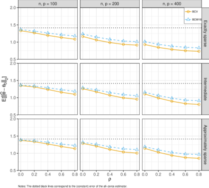
Figure 6.1 shows the mean 2subscript2\ell_{2} estimation error (for the slope coefficients, averaging over the 2,000 simulation draws) arising from BCV, post-BCV and CV, respectively, and using benchmark tuning.
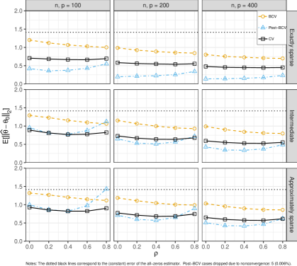
Figure 6.1: Mean 2subscript2\ell_{2} Estimation Error by Method with c0=1.1subscript𝑐01.1c_{0}=1.1 and αn=.1/ln(pn)subscript𝛼𝑛.1𝑝𝑛\alpha_{n}=.1/\ln\left(p\lor n\right)
Refer to caption

Mean 2subscript2\ell_{2} estimation error is here depicted as a function of the sample/problem size (the tile column), coefficient pattern (the tile row), and correlation level (the horizontal axis in each tile). We also include a horizontal line at 𝜽02subscriptnormsubscript𝜽02\|\bm{\theta}_{0}\|_{2}, which facilitates comparison with the trivial “estimator” 𝜽^𝟎^𝜽0\widehat{\bm{\theta}}\equiv\bm{0}.

One observation evident from this figure is that the error curves of BCV, post-BCV and CV can cross. Hence, these estimators cannot be ranked in terms of mean 2subscript2\ell_{2} estimation error, in general. However, for the largest sample/problem size considered, post-BCV outperforms CV for small to medium levels of correlation, and CV outperforms BCV.242424We reach qualitatively identical conclusions from inspecting the median 2subscript2\ell_{2} estimation errors. Hence, these findings are not limited to one particular feature of the error distributions. We omit the corresponding median plots due to their similarity with the mean error plots. Figures are available upon request.

Increasing the sample size (moving from left to right) leads to a downward shift in mean estimation error for all three estimators, which is indicative of convergence. Convergence appears to take place no matter the coefficient pattern or regressor correlation level even though the number of candidate regressors matches the sample size. Increasing the number of non-zeros in 𝜽0subscript𝜽0\bm{\theta}_{0} (moving from top to bottom) leads to an upward shift in mean estimation error. This finding is consistent with convergence slowing down with q𝑞q and sqsubscript𝑠𝑞s_{q} as predicted by Theorems 4.1 and 4.2.

We next investigate the impact of the choice of score markup c0subscript𝑐0c_{0}. Figures 6.2 and 6.3 plot the mean 2subscript2\ell_{2} estimation error for c0=1,1.05subscript𝑐011.05c_{0}=1,1.05 and (the previously used) 1.11.11.1, each sample/problem size and coefficient pattern, and for the BCV and post-BCV estimators, respectively.
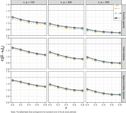
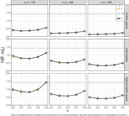
Figure 6.2: Mean 2subscript2\ell_{2} BCV Estimation Error by Score Markup with αn=.1/ln(pn)subscript𝛼𝑛.1𝑝𝑛\alpha_{n}=.1/\ln\left(p\lor n\right)
Refer to caption
Figure 6.3: Mean 2subscript2\ell_{2} Post-BCV Estimation Error by Score Markup with αn=.1/ln(pn)subscript𝛼𝑛.1𝑝𝑛\alpha_{n}=.1/\ln\left(p\lor n\right)
Refer to caption

Figure 6.2 suggests that increasing c0subscript𝑐0c_{0} away from one slightly worsens (mean estimation error) performance of BCV. While our theory takes c0subscript𝑐0c_{0} strictly greater than one, any value near one—including the limit case of one itself— appears to lead to near identical results.252525That mean BCV error is downward sloping for small to moderate ρ𝜌\rho levels is due to the signal being increasing in ρ𝜌\rho and need not translate to other correlation or coefficient patterns. For post-BCV (Figure 6.3), the findings are similar. In fact, at least for the largest sample/problem size, the exact value of c0{1,1.05,1.1}subscript𝑐011.051.1c_{0}\in\left\{1,1.05,1.1\right\} has little to no impact on mean error. Note that our findings for post-BCV apply even with the approximately sparse coefficient pattern, where variable selection mistakes are bound to occur. To conclude this subsection, we note that it is a well-known problem in the LASSO literature that the theory typically requires that c0subscript𝑐0c_{0} is strictly bigger than one, with the estimation error bounds deteriorating as c0subscript𝑐0c_{0} approaches one, but the simulation experience suggests that the estimation errors are insensitive with respect to c0subscript𝑐0c_{0} when c0subscript𝑐0c_{0} is close to one. We believe that solving this problem remains one of the key challenges in this literature.

6.3.3 Normal Approximation

We next assess the normal approximations resulting from three-step debiasing (Algorithm 5.1) using either BCV, post-BCV or CV. Instead of looking at the standardized estimate n(β^β0)/σ0𝑛^𝛽subscript𝛽0subscript𝜎0\sqrt{n}(\widehat{\beta}-\beta_{0})/\sigma_{0} for the true asymptotic variance σ02superscriptsubscript𝜎02\sigma_{0}^{2} given in (5.6), we form an estimate σ^2superscript^𝜎2\widehat{\sigma}^{2} and consider the studentized estimate n(β^β0)/σ^𝑛^𝛽subscript𝛽0^𝜎\sqrt{n}(\widehat{\beta}-\beta_{0})/\widehat{\sigma}. That is, we take into account the unknown nature of the σ02superscriptsubscript𝜎02\sigma_{0}^{2}, as required in an empirical application.

To construct the estimate σ^2superscript^𝜎2\widehat{\sigma}^{2}, we first leverage the binary response model to establish the (conditional information) equality E[m1(𝑿𝜽0,𝒀)2𝑿]=E[m11′′(𝑿𝜽0,𝒀)𝑿].Edelimited-[]conditionalsuperscriptsubscript𝑚1superscriptsuperscript𝑿topsubscript𝜽0𝒀2𝑿Edelimited-[]conditionalsuperscriptsubscript𝑚11′′superscript𝑿topsubscript𝜽0𝒀𝑿\mathrm{E}[m_{1}^{\prime}\left(\bm{X}^{\top}\bm{\theta}_{0},\bm{Y}\right)^{2}\mid\bm{X}]=\mathrm{E}[m_{11}^{\prime\prime}\left(\bm{X}^{\top}\bm{\theta}_{0},\bm{Y}\right)\mid\bm{X}]. We then use the definition of 𝝁0subscript𝝁0\bm{\mu}_{0} to establish the (weighted projection) equality

E[m11′′(𝑿𝜽0,𝒀)(D𝑾𝝁0)2]=E[m11′′(𝑿𝜽0,𝒀)(D𝑾𝝁0)D].Edelimited-[]superscriptsubscript𝑚11′′superscript𝑿topsubscript𝜽0𝒀superscript𝐷superscript𝑾topsubscript𝝁02Edelimited-[]superscriptsubscript𝑚11′′superscript𝑿topsubscript𝜽0𝒀𝐷superscript𝑾topsubscript𝝁0𝐷\mathrm{E}\big{[}m_{11}^{\prime\prime}\left(\bm{X}^{\top}\bm{\theta}_{0},\bm{Y}\right)\left(D-\bm{W}^{\top}\bm{\mu}_{0}\right)^{2}\big{]}=\mathrm{E}\left[m_{11}^{\prime\prime}\left(\bm{X}^{\top}\bm{\theta}_{0},\bm{Y}\right)\left(D-\bm{W}^{\top}\bm{\mu}_{0}\right)D\right].

Again using the binary response model, we can evaluate

E[m11′′(𝑿𝜽0,𝒀)𝑿𝜽0=t]=f(t)2F(t)(1F(t))=:ωF(t),\displaystyle\mathrm{E}\left[m_{11}^{\prime\prime}\left(\bm{X}^{\top}\bm{\theta}_{0},\bm{Y}\right)\mid\bm{X}^{\top}\bm{\theta}_{0}=t\right]=\frac{f\left(t\right)^{2}}{F\left(t\right)\left(1-F\left(t\right)\right)}=:\omega_{F}\left(t\right),

where f𝑓f and F𝐹F denote the PDF and CDF, respectively, associated with the binary response model.262626In our current binary probit setting, these functions are the standard normal PDF and CDF, respectively. In the empirical application in Section 7, we also use the logistic distribution, thus leading to the binary logit. This allows us to simplify the expression for σ02superscriptsubscript𝜎02\sigma_{0}^{2} to

σ02=1/E[ωF(𝑿𝜽0)(D𝑾𝝁0)D]superscriptsubscript𝜎021Edelimited-[]subscript𝜔𝐹superscript𝑿topsubscript𝜽0𝐷superscript𝑾topsubscript𝝁0𝐷\sigma_{0}^{2}=1\big{/}\mathrm{E}\left[\omega_{F}\left(\bm{X}^{\top}\bm{\theta}_{0}\right)\left(D-\bm{W}^{\top}\bm{\mu}_{0}\right)D\right]

and leads to the following estimator of σ02superscriptsubscript𝜎02\sigma_{0}^{2}:

σ^2:=1/𝔼n[ωF(β^Di+𝑾i𝜸~)(Di𝑾i𝝁~)Di],assignsuperscript^𝜎21subscript𝔼𝑛delimited-[]subscript𝜔𝐹^𝛽subscript𝐷𝑖superscriptsubscript𝑾𝑖top~𝜸subscript𝐷𝑖superscriptsubscript𝑾𝑖top~𝝁subscript𝐷𝑖\widehat{\sigma}^{2}:=1\big{/}\mathbb{E}_{n}\big{[}\omega_{F}\big{(}\widehat{\beta}D_{i}+\bm{W}_{i}^{\top}\widetilde{\bm{\gamma}}\big{)}\big{(}D_{i}-\bm{W}_{i}^{\top}\widetilde{\bm{\mu}}\big{)}D_{i}\big{]},

with 𝜸~,𝝁~~𝜸~𝝁\widetilde{\bm{\gamma}},\widetilde{\bm{\mu}} and β^^𝛽\widehat{\beta} given by Steps 1, 2 and 3, respectively, of Algorithm 5.1 given different rules for choosing the penalties λ1subscript𝜆1\lambda_{1} and λ2subscript𝜆2\lambda_{2}.272727Alternatively, one can use the “sandwich” estimators (5.7) and (5.8). Experimenting with these estimators, we obtained numerically similar results as reported below for the estimator σ^2superscript^𝜎2\widehat{\sigma}^{2}. We prefer σ^2superscript^𝜎2\widehat{\sigma}^{2} since it leverages both the binary response and projection structure.

Figure 6.4 shows the (kernel) densities of the studentized estimates using benchmark tuning and ρ=0𝜌0\rho=0.282828All kernel densities are created using the R package ggplot2 with geom_density. In expectation of an approximately normal distribution, we use a Gaussian kernel and the Silverman (1986, Equation (3.31)) rule-of-thumb bandwidth (both geom_density defaults), which is optimal for the Gaussian distribution.

Figure 6.4: Densities of Studentized Estimates by n(=p)annotated𝑛absent𝑝n(=p) with ρ=0𝜌0\rho=0, c0=1.1subscript𝑐01.1c_{0}=1.1 and αn=.1/ln(pn)subscript𝛼𝑛.1𝑝𝑛\alpha_{n}=.1/\ln\left(p\lor n\right).
Refer to caption

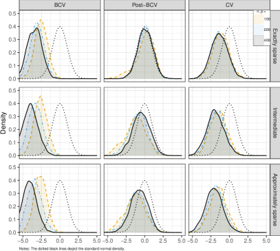
The densities arising from BCV, post-BCV and CV, respectively, are here depicted as columns of tiles, where each tile row corresponds to a coefficient pattern and each graph within a tile a sample/problem size. Starting with the exactly sparse coefficient pattern (the top row of tiles), we see that both BCV and CV lead to considerable shrinkage bias even after debiasing the initial estimate of the focal parameter β0subscript𝛽0\beta_{0}. This feature is seen from the leftward shifts in the resulting densities compared to the standard normal density, here represented by the dotted line. Note that these biases do not disappear as the sample size grows without bound. If anything, these distributions shift further left as n𝑛n increases, holding n=p𝑛𝑝n=p. In constrast, the post-BCV density essentially collapses to the standard normal one, at least for n=p=200𝑛𝑝200n=p=200 and 400400400.

As the coefficient pattern becomes less and less sparse (moving down), all approximations deteriorate, as is to be expected. While imperfect, the post-BCV densities are still decent approximations to the normal for both the intermediate and approximately sparse coefficient patterns. Moreover, only these densities appear to approach the standard normal as the sample/problem size increases.

While Figure 6.4 depicts the normal approximations for ρ=0𝜌0\rho=0 (the worst-correlation case), in Figure 6.5 we display the normal approximations as a function of ρ𝜌\rho.

Figure 6.5: Densities of Studentized Post-BCV and CV Estimates for Different ρ𝜌\rho with n(=p)=400,annotated𝑛absent𝑝400n(=p)=400, Approximately Sparse Coefficient Pattern, c0=1.1subscript𝑐01.1c_{0}=1.1 and αn=.1/ln(pn)subscript𝛼𝑛.1𝑝𝑛\alpha_{n}=.1/\ln\left(p\lor n\right)
Refer to caption

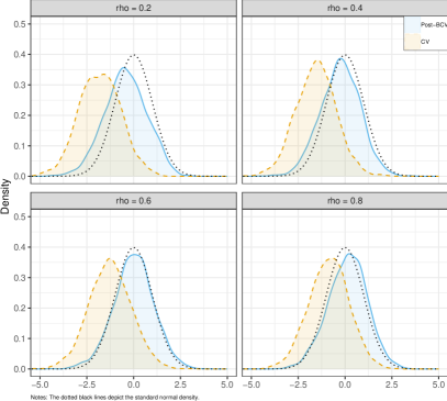
We here focus on the largest sample size n(=p)=400annotated𝑛absent𝑝400n(=p)=400 and the (more challenging) approximately sparse coefficient pattern, again using benchmark tuning. Since post-BCV and CV appear to lead to better normal approximations than BCV, we display only results from the former two methods. Post-BCV leads to a relatively accurate normal approximation for every correlation level considered. Moreover, while the normal approximation stemming from CV appears to improve as ρ𝜌\rho increases, at no correlation level considered does CV lead to a visually better approximation than post-BCV.292929We also investigated the robustness of the post-BCV-resulting normal approximations with respect to the markup c0{1,1.05,1.1}subscript𝑐011.051.1c_{0}\in\{1,1.05,1.1\}. Parallelling our findings for mean estimation error in Figure 6.3, the exact markup value appears to make little difference. (Figures are available upon request.)

7 Revisiting Racial Differences in Police Use of Force

In this section we revisit the empirical setting in Fryer Jr (2019) (henceforth: Fryer), who explored racial differences in police use of force. We here focus on the part of Fryer’s regression analysis invoking the full Police-Public Contact Survey (PPCS) dataset with the outcome being an indicator for any use of force by the police (conditional on a encounter), thus leading to a binary response model as in our Example 1.303030See Fryer Jr (2019) and the associated online appendix for alternative outcome variables and data sources as well as a detailed discussion of their relative merits and drawbacks. Specifically, Fryer estimates models of the form

P(Force=1𝐑𝐚𝐜𝐞,𝑾)=F(𝐑𝐚𝐜𝐞𝜶0+𝑾𝜸0),PForceconditional1𝐑𝐚𝐜𝐞𝑾𝐹superscript𝐑𝐚𝐜𝐞topsubscript𝜶0superscript𝑾topsubscript𝜸0\mathrm{P}\left(\mathrm{Force}=1\mid\mathbf{Race},\bm{W}\right)=F\left(\mathbf{Race}^{\top}\bm{\alpha}_{0}+\bm{W}^{\top}\bm{\gamma}_{0}\right), (7.1)

where ForceForce\mathrm{Force} indicates whether any force was used by the police when encountering a civilian, 𝐑𝐚𝐜𝐞=(Black,Hisp,Other)𝐑𝐚𝐜𝐞superscriptBlackHispOthertop\mathbf{Race}=(\mathrm{Black},\mathrm{Hisp},\mathrm{Other})^{\top} indicate the race of the civilian (black, hispanic and other than white, with white being the reference race), and 𝑾𝑾\bm{W} is a list of control variables capturing both civilian (e.g. gender and age), officer (e.g. majority race) and encounter characteristics (e.g. whether the civilian disobeyed, resisted or otherwise misbehaved).313131See the Fryer Jr (2019, Table 2.B) notes for the full variable list and his online appendix A for descriptions. Here F𝐹F is a placeholder for a strictly increasing known cumulative distribution function (CDF), which Fryer takes to be the logistic CDF ΛΛ\Lambda, thus leading to the binary logit model.

The PPCS logistic regression results reported in Fryer Jr (2019, Table 2.B) show that black and hispanic subjects are statistically significantly more likely to experience some form of force in interactions with the police, controlling for context and civilian behavior. We here look into the robustness of this finding by employing also (i) an alternative binary response model and (ii) large(r) sets of candidate regressors, in combination with 1subscript1\ell_{1}-penalization. For brevity, we here single out the black dummy (Black)Black(\mathrm{Black}) and its coefficient βBlacksubscript𝛽Black\beta_{\mathrm{Black}} and group the other non-white dummies (HispHisp\mathrm{Hisp} and OtherOther\mathrm{Other}) with the controls (thus recasting 𝜸0subscript𝜸0\bm{\gamma}_{0}). We interpret the statement “there are no racial differences in police use of force” as there being no difference in the probability of force being used for black civilians relative to white subjects, holding everything else equal. That is,

P(Force=1Black=1,𝑾=𝒘)=P(Force=1Black=0,𝑾=𝒘)\mathrm{P}\left(\mathrm{Force}=1\mid\mathrm{Black}=1,\bm{W}=\bm{w}\right)=\mathrm{P}\left(\mathrm{Force}=1\mid\mathrm{Black}=0,\bm{W}=\bm{w}\right)

for all realizations of the controls 𝒘𝒘\bm{w} (with HispHisp\mathrm{Hisp} and OtherOther\mathrm{Other} both zero). Since the race dummies enter the strictly increasing F𝐹F in (7.1) in an additive manner, such a zero probability difference is equivalent to a zero coefficient on the dummy for being black, i.e. βBlack=0subscript𝛽Black0\beta_{\mathrm{Black}}=0. We therefore take the latter as the hypothesis to be tested.

First, using the Fryer Jr (2019) supplementary files and descriptions in his online appendix, we recollect and recreate the PPCS dataset. Using the same supplementary files, we then replicate the PPCS logistic regression results in Fryer Jr (2019, Table 2.B) to all reported digits, which leaves us confident that we are indeed considering the original dataset.

We next apply three-step debiasing (Algorithm 5.1) with the loss function being either the negative logit or probit log-likelihood. Our simulation findings indicate that post-BCV debiasing outperforms both the BCV and CV equivalents. We therefore only consider the former. We use two sets of regressors. The first set (Basic Controls) corresponds to that in Fryer Jr (2019, Table 2.B, Row l), which is Fryer’s largest set of controls. The only difference is that we include categorical regressors via dummies for their different levels, leaving one reference category for each. The second set of regressors (Basic Controls + Interactions) builds on the first by adding all first-order pairwise interactions between the controls (excluding the race dummies HispHisp\mathrm{Hisp} and OtherOther\mathrm{Other}). After eliminating variables with zero variance or perfect correlation, the two sets include 31 and 345 non-constant regressors, respectively, which should be compared to a sample size of n=59,668𝑛59668n=59,668 civilian–police encounters.323232We note in passing that the 59,668 equals the total number of police-civilian encounters in the PPCS dataset covering the six surveys 1996, 1999, 2002, 2005, 2008 and 2011. The number of complete cases with respect to the regressors used is 9,930 and only leaves the years 2002 and 2011. For a clean comparison, we follow Fryer’s approach to missing values.

Table 1 displays the t𝑡t-statistics associated with testing the null hypothesis using either unpenalized or 1subscript1\ell_{1}-penalized methods.

Table 1: t𝑡t-Statistic for Testing a Zero Coefficient βBlacksubscript𝛽Black\beta_{\mathrm{Black}} on BlackBlack\mathrm{Black}
Unpenalized (ML) Post-BCV
Controls \ Loss Logit Probit Logit Probit
Basic Controls 8.7 8.7 10.5 9.6
+ Interactions n.a. n.a. 20.7 18.9

Using only basic controls (the logit case being covered in Fryer), the t𝑡t-statistics take on similar values for both unpenalized maximum likelihood (ML) and post-BCV methods. Thus, with only 31 candidate regressors, regularization has little impact. In contrast, the specification including both basic controls and interactions thereof leads to complete separation in the data, such that the (unpenalized) maximum likelihood estimates do not exist (as real numbers). For this case, some regularization is necessary. Hence, although the numbers of regressors considered here may not appear overwhelmingly large when compared to the sample size, the set of regressors is of great importance. Even when we include all first-order interactions between the controls, the t𝑡t-statistics resulting from our three-step debiasing procedure remain of the same order as before.333333The increase in the t𝑡t-statistic values for post-BCV arising from inclusion of interactions is for both the logit and probit loss due to both a somewhat larger coefficient estimate and a somewhat smaller standard error. The values underlying Table 1 therefore illustrate that a larger set of candidate regressors need not lead to larger estimation error. The t𝑡t-tests based on our post-BCV debiasing lead us to reject the null hypothesis of no racial differences in police use of force at any reasonable significance level. This conclusion in Fryer Jr (2019) therefore appears robust to the choice of controls.

To gauge the economic impact of our change in estimation procedures, we estimate the average partial effect (APE) of changing the civilian race from white to black. Iterating expectations and using (7.1), the theoretical APE can be expressed as the average probability difference

APEBlacksubscriptAPEBlack\displaystyle\mathrm{APE}_{\mathrm{Black}} :=E[P(Force=1Black=1,Hisp=0,Other=0,𝑾)\displaystyle:=\mathrm{E}\big{[}\mathrm{P}\left(\mathrm{Force}=1\mid\mathrm{Black}=1,\mathrm{Hisp}=0,\mathrm{Other}=0,\bm{W}\right)
P(Force=1Black=0,Hisp=0,Other=0,𝑾)]\displaystyle\quad\quad-\mathrm{P}\left(\mathrm{Force}=1\mid\mathrm{Black}=0,\mathrm{Hisp}=0,\mathrm{Other}=0,\bm{W}\right)\big{]}
=E[F(βBlack+𝑾𝜸0)F(𝑾𝜸0)],absentEdelimited-[]𝐹subscript𝛽Blacksuperscript𝑾topsubscript𝜸0𝐹superscript𝑾topsubscript𝜸0\displaystyle=\mathrm{E}\left[F\left(\beta_{\mathrm{Black}}+\bm{W}^{\top}\bm{\gamma}_{0}\right)-F\left(\bm{W}^{\top}\bm{\gamma}_{0}\right)\right], (7.2)

where we bring back the other (non-white) civilian race dummies to clarify the comparison made. We estimate this APE by APE^Black:=𝔼n[F(β^Black+𝑾i𝜸^)F(𝑾i𝜸^)],assignsubscript^APEBlacksubscript𝔼𝑛delimited-[]𝐹subscript^𝛽Blacksuperscriptsubscript𝑾𝑖top^𝜸𝐹superscriptsubscript𝑾𝑖top^𝜸\widehat{\mathrm{APE}}_{\mathrm{Black}}:=\mathbb{E}_{n}[F\big{(}\widehat{\beta}_{\mathrm{Black}}+\bm{W}_{i}^{\top}\widehat{\bm{\gamma}}\big{)}-F\left(\bm{W}_{i}^{\top}\widehat{\bm{\gamma}}\right)], for point estimates β^Blacksubscript^𝛽Black\widehat{\beta}_{\mathrm{Black}} and 𝜸^^𝜸\widehat{\bm{\gamma}} of βBlacksubscript𝛽Black\beta_{\mathrm{Black}} and 𝜸0subscript𝜸0\bm{\gamma}_{0}, respectively. When results stem from (unpenalized) ML, we use the ML estimates. When results stem from three-step post-BCV debiasing, we use the debiased third-step estimate for β^Blacksubscript^𝛽Black\widehat{\beta}_{\mathrm{Black}} and use the (biased) first-step estimate of 𝜸0subscript𝜸0\bm{\gamma}_{0} for 𝜸^^𝜸\widehat{\bm{\gamma}}. Table 2 reports the APE estimates (in percentage points) corresponding to these procedures including either basic controls or basic controls with interactions.

Table 2: Estimates of the Average Partial Effect of Black (in Percentage Points)
100×APEBlack100subscriptAPEBlack100\times\mathrm{APE}_{\mathrm{Black}} Unpenalized (ML) Post-BCV
Controls \ Loss Logit Probit Logit Probit
Basic Controls 1.1 1.1 1.4 1.3
+ Interactions n.a. n.a. 3.2 2.8

Using only basic controls, (unpenalized) ML and post-BCV lead to APE estimates in the range of 1.1-1.4 percentage points regardless of the CDF used. For context, the unconditional average of contacts in which PPCS respondents reported any force being used for white civilians is .7 percent. Including interactions of basic controls, the post-BCV APE estimates roughly double in size to about 3 percentage points. Of course, these relatively large APE estimates may come with relatively large estimation error. However, as the APE in (7.2) depends on many (in fact, nearly all) the unknown coefficients, it remains a non-trivial task to assign standard errors to these point estimates—a task falling outside the scope of this paper.

Finally, to illustrate the computational burden associated with the methods proposed in this paper when applied to real data, in Table 3 we report the computing time used by the above-mentioned estimation routines.

Table 3: Estimation Routine Timings (in Seconds)
Unpenalized (ML) Post-BCV
Controls \ Loss Logit Probit Logit Probit
Basic Controls 1.37 1.41 18.4 38.2
+ Interactions \infty \infty 211.8 199.2
  • Notes: All timings were carried out on an Intel Core i7-8700 3.20GHz CPU. When using cv.glmnet, we use the parallel computing option with all 12 virtual cores available.

With only 31 basic controls, the three-step post-BCV debiasing procedure takes at least ten times as long as (unpenalized) ML. This is not too surprising, as the former method involves two rounds of CV, bootstrapping and refitting—no task of which is undertaken by ML. However, including also basic control interactions (bringing the number of controls to 328), the ranking of the two approaches is reversed. The roughly tenfold (328/3110.6)3283110.6(328/31\approx 10.6) increase in number of controls increases the computing time associated with post-BCV logit debiasing by 211.8/18.411.5211.818.411.5211.8/18.4\approx 11.5, i.e. almost linearly. For post-BCV probit debiasing, the corresponding increase is about five fold (199.2/38.25.2)199.238.25.2(199.2/38.2\approx 5.2). In contrast, as the ML estimates are not real numbers, without proper checks for existence of a solution, any (gradient-based) optimizer would have to iterate indefinitely in an attempt to obtain the ML estimates. We here represent the non-existence of an ML estimate by an infinite computing time.343434While infinite time may appear overly dramatic, we warn that glmnet does not check for divergence of the optimization algorithm (cf. Friedman et al., 2010, p. 9). For this reason we opted for stats::glm for ML estimation and refitting after variable selection.

Of course, the particular runtimes reported in Table 3 are only single observations arising from a particular implementation of our procedures and using a specific dataset and our specific computing environment. As such, they need not be representative of the runtimes that would expect in other environments or applications.

References

  • Adler and Taylor (2007) Adler, R. J. and J. E. Taylor (2007): Random fields and geometry, Springer Science & Business Media.
  • Aigner et al. (1976) Aigner, D. J., T. Amemiya, and D. J. Poirier (1976): “On the estimation of production frontiers: maximum likelihood estimation of the parameters of a discontinuous density function,” International Economic Review, 377–396.
  • Ali and Tibshirani (2019) Ali, A. and R. J. Tibshirani (2019): “The Generalized Lasso Problem and Uniqueness,” Electronic Journal of Statistics, 13, 2307–2347, publisher: Institute of Mathematical Statistics and Bernoulli Society.
  • Belloni et al. (2012) Belloni, A., D. Chen, V. Chernozhukov, and C. Hansen (2012): “Sparse models and methods for optimal instruments with an application to eminent domain,” Econometrica, 80, 2369–2429.
  • Belloni et al. (2017) Belloni, A., K. Chernozhukov, and K. Kato (2017): “High-dimensional quantile regression,” Handbook of Quantile Regression.
  • Belloni and Chernozhukov (2011a) Belloni, A. and V. Chernozhukov (2011a): High dimensional sparse econometric models: An introduction, Springer.
  • Belloni and Chernozhukov (2011b) ——— (2011b): “l1-penalized quantile regression in high-dimensional sparse models,” The Annals of Statistics, 39, 82–130.
  • Belloni and Chernozhukov (2013) ——— (2013): “Least squares after model selection in high-dimensional sparse models,” Bernoulli, 19, 521–547.
  • Belloni et al. (2023) Belloni, A., V. Chernozhukov, D. Chetverikov, C. Hansen, and K. Kato (2023): “High-dimensional econometrics and regularized GMM,” Working Paper.
  • Belloni et al. (2015) Belloni, A., V. Chernozhukov, D. Chetverikov, and K. Kato (2015): “Some new asymptotic theory for least squares series: Pointwise and uniform results,” Journal of Econometrics, 186, 345–366.
  • Belloni et al. (2018) Belloni, A., V. Chernozhukov, D. Chetverikov, and Y. Wei (2018): “Uniformly valid post-regularization confidence regions for many functional parameters in z-estimation framework,” Annals of statistics, 46, 3643.
  • Belloni et al. (2016) Belloni, A., V. Chernozhukov, and Y. Wei (2016): “Post-selection inference for generalized linear models with many controls,” Journal of Business & Economic Statistics, 34, 606–619.
  • Bickel et al. (2009) Bickel, P. J., Y. Ritov, and A. B. Tsybakov (2009): “Simultaneous analysis of Lasso and Dantzig selector,” The Annals of Statistics, 1705–1732.
  • Buchinsky and Hahn (1998) Buchinsky, M. and J. Hahn (1998): “An alternative estimator for the censored quantile regression model,” Econometrica, 653–671.
  • Candes and Tao (2007) Candes, E. and T. Tao (2007): “The Dantzig selector: statistical estimation when p is much larger than n,” The Annals of Statistics, 2313–2351.
  • Chamberlain (1984) Chamberlain, G. (1984): “Panel data,” Handbook of econometrics, 2, 1247–1318.
  • Chamberlain (1985) ——— (1985): “Heterogeneity, omitted variable bias, and duration dependence,” in Longitudinal Analysis of Labor Market Data, ed. by J. J. Heckman and B. Singer, Cambridge University Press, 3–38.
  • Chernozhukov et al. (2018) Chernozhukov, V., D. Chetverikov, M. Demirer, E. Duflo, C. Hansen, W. Newey, and J. Robins (2018): “Double/debiased machine learning for treatment and structural parameters,” The Econometrics Journal, 21, C1–C68.
  • Chernozhukov et al. (2013) Chernozhukov, V., D. Chetverikov, and K. Kato (2013): “Gaussian approximations and multiplier bootstrap for maxima of sums of high-dimensional random vectors,” The Annals of Statistics, 41, 2786–2819.
  • Chernozhukov et al. (2017) ——— (2017): “Central limit theorems and bootstrap in high dimensions,” The Annals of Probability, 45, 2309–2352.
  • Chetverikov et al. (2021) Chetverikov, D., Z. Liao, and V. Chernozhukov (2021): “On cross-validated Lasso,” Annals of Statistics, 49, 1300–1317.
  • de la Pena et al. (2009) de la Pena, V. H., T. L. Lai, and Q.-M. Shao (2009): Self-normalized processes. Probability and its Applications, New York. Springer-Verlag, Berlin.
  • Dudley (2014) Dudley, R. (2014): Uniform Central Limit Theorems, 142, Cambridge University Press.
  • Friedman et al. (2010) Friedman, J., T. Hastie, and R. Tibshirani (2010): “Regularization paths for generalized linear models via coordinate descent,” Journal of statistical software, 33, 1.
  • Fryer Jr (2019) Fryer Jr, R. G. (2019): “An empirical analysis of racial differences in police use of force,” Journal of Political Economy, 127, 1210–1261, publisher: The University of Chicago Press Chicago, IL.
  • Hastie et al. (2015) Hastie, T., R. Tibshirani, and M. Wainwright (2015): Statistical Learning with Sparsity: The Lasso and Generalizations, CRC Press.
  • Honoré (1992) Honoré, B. E. (1992): “Trimmed LAD and least squares estimation of truncated and censored regression models with fixed effects,” Econometrica: journal of the Econometric Society, 533–565.
  • Imai and Ratkovic (2014) Imai, K. and M. Ratkovic (2014): “Covariate balancing propensity score,” Journal of the Royal Statistical Society: Series B (Statistical Methodology), 76, 243–263.
  • Javanmard and Montanari (2013) Javanmard, A. and A. Montanari (2013): “Confidence intervals and hypothesis testing for high-dimensional statistical models,” Advances in neural information processing systems, 26.
  • Jing et al. (2003) Jing, B.-Y., Q.-M. Shao, and Q. Wang (2003): “Self-normalized Cramér-type large deviations for independent random variables,” The Annals of probability, 31, 2167–2215, publisher: Institute of Mathematical Statistics.
  • Lancaster (1992) Lancaster, T. (1992): The econometric analysis of transition data, 17, Cambridge university press.
  • Lecue and Mitchell (2012) Lecue, G. and G. Mitchell (2012): “Oracle inequalities for cross-validation type procedures,” Electronic Journal of Statistics, 1803–1837.
  • Meinshausen (2007) Meinshausen, N. (2007): “Relaxed lasso,” Computational Statistics & Data Analysis, 52, 374–393.
  • Miolane and Montanari (2018) Miolane, L. and A. Montanari (2018): “The distribution of the Lasso: uniform control over sparse balls and adaptive parameter tuning,” arXiv:1811.01212.
  • Negahban et al. (2012) Negahban, S. N., P. Ravikumar, M. J. Wainwright, and B. Yu (2012): “A unified framework for high-dimensional analysis of $ M $-estimators with decomposable regularizers,” Statistical science, 27, 538–557, publisher: Institute of Mathematical Statistics.
  • Newey and Powell (1987) Newey, W. K. and J. L. Powell (1987): “Asymmetric least squares estimation and testing,” Econometrica: Journal of the Econometric Society, 819–847.
  • Ng (2004) Ng, A. Y. (2004): “Feature selection, L 1 vs. L 2 regularization, and rotational invariance,” in Proceedings of the twenty-first international conference on Machine learning, ACM, 78.
  • Ninomiya and Kawano (2016) Ninomiya, Y. and S. Kawano (2016): “AIC for the Lasso in generalized linear models,” Electronic Journal of Statistics.
  • Osborne et al. (2000) Osborne, M. R., B. Presnell, and B. A. Turlach (2000): “On the lasso and its dual,” Journal of Computational and Graphical statistics, 9, 319–337.
  • Pratt (1981) Pratt, J. W. (1981): “Concavity of the log likelihood,” Journal of the American Statistical Association, 76, 103–106, publisher: Taylor & Francis.
  • Rasch (1960) Rasch, G. (1960): Probabilistic Models for Some Intelligence and Attainment Tests, Studies in mathematical psychology, Danmarks Paedagogiske Institut.
  • Raskutti et al. (2011) Raskutti, G., M. Wainwright, and B. Yu (2011): “Minimax rates of estimation for high-dimensional linear regression over qsubscript𝑞\ell_{q} balls,” IEEE Trans. Inform. Theory, 57, 6976–6994.
  • Rockafellar (1970) Rockafellar, R. T. (1970): “Convex Analysis (Princeton Mathematical Series),” Princeton University Press, 46, 49.
  • Rosset et al. (2004) Rosset, S., J. Zhu, and T. Hastie (2004): “Boosting as a regularized path to a maximum margin classifier,” The Journal of Machine Learning Research, 5, 941–973, publisher: JMLR. org.
  • Silverman (1986) Silverman, B. W. (1986): Density Estimation for Statistics and Data Analysis, vol. 26 of Monographs on Statistics and Applied Probability, London: Chapman & Hall, publisher: Chapman and Hall.
  • Sørensen (2022) Sørensen, J. R.-V. (2022): “Testing a Class of Semi- or Nonparametric Conditional Moment Restriction Models using Series Methods,” Econometric Theory, 1–32.
  • Talagrand (2010) Talagrand, M. (2010): Mean field models for spin glasses: Volume I: Basic examples, vol. 54, Springer Science & Business Media.
  • Tan (2020) Tan, Z. (2020): “Regularized calibrated estimation of propensity scores with model misspecification and high-dimensional data,” Biometrika, 107, 137–158.
  • Tibshirani (1996) Tibshirani, R. (1996): “Regression shrinkage and selection via the lasso,” Journal of the Royal Statistical Society. Series B (Methodological), 267–288.
  • Tibshirani (2013) Tibshirani, R. J. (2013): “The lasso problem and uniqueness,” Electronic Journal of Statistics, 7, 1456–1490, publisher: Institute of Mathematical Statistics and Bernoulli Society.
  • Tsybakov (2004) Tsybakov, A. B. (2004): “Optimal aggregation of classifiers in statistical learning,” The Annals of Statistics, 32, 135–166, publisher: Institute of Mathematical Statistics.
  • van de Geer (2016) van de Geer, S. (2016): “Estimation and testing under sparsity,” Lecture notes in mathematics, 2159, publisher: Springer.
  • van de Geer et al. (2014) van de Geer, S., P. Bühlmann, Y. Ritov, and R. Dezeure (2014): “On asymptotically optimal confidence regions and tests for high-dimensional models,” The Annals of Statistics, 42, 1166 – 1202.
  • van de Geer (2008) van de Geer, S. A. (2008): “High-Dimensional Generalized Linear Models and the Lasso,” The Annals of Statistics, 36, 614–645.
  • van der Vaart and Wellner (1996) van der Vaart, A. W. and J. A. Wellner (1996): Weak Convergence and Empirical Processes, Springer.
  • Wainwright (2019) Wainwright, M. J. (2019): High-dimensional statistics: A non-asymptotic viewpoint, vol. 48, Cambridge University Press.
  • Wang et al. (2020) Wang, L., B. Peng, J. Bradic, R. Li, and Y. Wu (2020): “A tuning-free robust and efficient approach to high-dimensional regression,” Journal of the American Statistical Association, 115, 1700–1714, publisher: Taylor & Francis.
  • Wooldridge (2010) Wooldridge, J. M. (2010): Econometric analysis of cross section and panel data, MIT press.
\doparttoc\faketableofcontents

Online Appendices

\parttoc

Appendix A Verification of High-Level Assumptions

In this section, we discuss high-level assumptions from the main text. We first consider the case of linear models and the square loss, and then turn to the examples from Section 2. In particular, Corollaries A.1 and A.2 state convergence rate and inference results under low-level conditions for each of the examples from Section 2.

A.1 Verification for Linear Model with Square Loss

It is instructive to illustrate the contents of Assumptions 3.13.5, 4.1, 4.4, 4.5, 5.1, 5.3, and 5.4 in the familiar case of the linear mean model. We here consider the following (strong) version of the linear model with independent Gaussian errors,

Y=𝑿𝜽0+ε,ε𝑿N(0,σ02),formulae-sequence𝑌𝑿superscriptsubscript𝜽0top𝜀similar-toconditional𝜀𝑿N0superscriptsubscript𝜎02Y=\bm{X}{{}^{\top}}\bm{\theta}_{0}+\varepsilon,\quad\varepsilon\mid\bm{X}\sim\mathrm{N}\left(0,\sigma_{0}^{2}\right),

where θ0psubscript𝜃0superscript𝑝\theta_{0}\in\mathbb{R}^{p} and σ02(0,)superscriptsubscript𝜎020\sigma_{0}^{2}\in(0,\infty) are model parameters, and we use the square loss m(t,y)=(1/2)(yt)2𝑚𝑡𝑦12superscript𝑦𝑡2m(t,y)=(1/2)(y-t)^{2}. Less restrictive dependence and distributional assumptions can be accommodated. We focus on the independent Gaussian case for simplicity.

We take ΘΘ\Theta to be the full space psuperscript𝑝\mathbb{R}^{p}, such that Assumption 3.1 is trivial. Convexity of the loss (Assumption 3.2) follows from differentiating twice with respect to t𝑡t and observing that m11′′(t,y)=1>0subscriptsuperscript𝑚′′11𝑡𝑦10m^{\prime\prime}_{11}(t,y)=1>0 no matter (t,y)2𝑡𝑦superscript2(t,y)\in\mathbb{R}^{2}. For 𝜽Θ𝜽Θ\bm{\theta}\in\Theta arbitrary, the derivative m1(𝑿𝜽,Y)=𝑿𝜽0Y=εsuperscriptsubscript𝑚1superscript𝑿top𝜽𝑌superscript𝑿topsubscript𝜽0𝑌𝜀m_{1}^{\prime}(\bm{X}^{\top}\bm{\theta},Y)=\bm{X}^{\top}\bm{\theta}_{0}-Y=-\varepsilon surely exists. Denoting 𝜹:=𝜽𝜽0assign𝜹𝜽subscript𝜽0\bm{\delta}:=\bm{\theta}-\bm{\theta}_{0}, the finiteness of

E[|m(𝑿𝜽,Y)|]=12E[(ε𝑿𝜹)2]=12(σ02+𝜹E[𝑿𝑿]𝜹)Edelimited-[]𝑚superscript𝑿top𝜽𝑌12Edelimited-[]superscript𝜀superscript𝑿top𝜹212superscriptsubscript𝜎02superscript𝜹topEdelimited-[]𝑿superscript𝑿top𝜹\mathrm{E}\left[\left|m\left(\bm{X}^{\top}\bm{\theta},Y\right)\right|\right]=\frac{1}{2}\mathrm{E}\big{[}\left(\varepsilon-\bm{X}^{\top}\bm{\delta}\right)^{2}\big{]}=\frac{1}{2}\left(\sigma_{0}^{2}+\bm{\delta}^{\top}\mathrm{E}\left[\bm{X}\bm{X}^{\top}\right]\bm{\delta}\right)

hinges on finiteness of the matrix E[𝑿𝑿]Edelimited-[]𝑿superscript𝑿top\mathrm{E}[\bm{X}\bm{X}^{\top}]. In particular, Assumption 3.3 can be guaranteed by finiteness of second moments E[Xj2]Edelimited-[]superscriptsubscript𝑋𝑗2\mathrm{E}[X_{j}^{2}] for all j[p]𝑗delimited-[]𝑝j\in[p]. The excess risk at 𝜽𝜽\bm{\theta} is

(𝜽)=12E[(ε𝑿𝜹)2ε2]=12𝜹E[𝑿𝑿]𝜹12λmin(E[𝑿𝑿])𝜹22,𝜽12Edelimited-[]superscript𝜀superscript𝑿top𝜹2superscript𝜀212superscript𝜹topEdelimited-[]𝑿superscript𝑿top𝜹12subscript𝜆Edelimited-[]𝑿superscript𝑿topsuperscriptsubscriptnorm𝜹22\mathcal{E}\left(\bm{\theta}\right)=\frac{1}{2}\mathrm{E}\big{[}\left(\varepsilon-\bm{X}^{\top}\bm{\delta}\right)^{2}-\varepsilon^{2}\big{]}=\frac{1}{2}\bm{\delta}^{\top}\mathrm{E}\left[\bm{X}\bm{X}^{\top}\right]\bm{\delta}\geqslant\frac{1}{2}\lambda_{\min}\left(\mathrm{E}\left[\bm{X}\bm{X}^{\top}\right]\right)\left\|\bm{\delta}\right\|_{2}^{2},

with λmin(E[𝑿𝑿])subscript𝜆Edelimited-[]𝑿superscript𝑿top\lambda_{\min}(\mathrm{E}[\bm{X}\bm{X}^{\top}]) denoting the smallest eigenvalue of E[𝑿𝑿]Edelimited-[]𝑿superscript𝑿top\mathrm{E}[\bm{X}\bm{X}^{\top}]. As long as the eigenvalues are bounded away from zero, Assumption 3.4 holds with cM=1(1/2)infnλmin(E[𝑿𝑿])subscript𝑐𝑀112subscriptinfimum𝑛subscript𝜆Edelimited-[]𝑿superscript𝑿topc_{M}=1\wedge(1/2)\inf_{n\in\mathbb{N}}\lambda_{\min}(\mathrm{E}[\bm{X}\bm{X}^{\top}]) and cM=superscriptsubscript𝑐𝑀c_{M}^{\prime}=\infty. Positivity of λmin(E[𝑿𝑿])subscript𝜆Edelimited-[]𝑿superscript𝑿top\lambda_{\min}(\mathrm{E}[\bm{X}\bm{X}^{\top}]) is precisely the rank condition for identification of 𝜽0subscript𝜽0\bm{\theta}_{0}. Without this condition 𝜽0subscript𝜽0\bm{\theta}_{0} does not uniquely minimize the expected loss. Turning to Assumption 3.5.1, a calculation shows that for all (𝒙,y)p+1𝒙𝑦superscript𝑝1(\bm{x},y)\in\mathbb{R}^{p+1} and all (t1,t2)2subscript𝑡1subscript𝑡2superscript2(t_{1},t_{2})\in\mathbb{R}^{2},

|m(𝒙𝜽0+t1,y)m(𝒙𝜽0+t2,y)|𝑚superscript𝒙topsubscript𝜽0subscript𝑡1𝑦𝑚superscript𝒙topsubscript𝜽0subscript𝑡2𝑦\displaystyle\left\lvert m\left(\bm{x}^{\top}\bm{\theta}_{0}+t_{1},y\right)-m\left(\bm{x}^{\top}\bm{\theta}_{0}+t_{2},y\right)\right\rvert =12|t1+t2+2(𝒙𝜽0y)||t1t2|absent12subscript𝑡1subscript𝑡22superscript𝒙topsubscript𝜽0𝑦subscript𝑡1subscript𝑡2\displaystyle=\frac{1}{2}\left|t_{1}+t_{2}+2\left(\bm{x}^{\top}\bm{\theta}_{0}-y\right)\right|\left|t_{1}-t_{2}\right|
12(|t1|+|t2|+2|y𝒙𝜽0|)|t1t2|.absent12subscript𝑡1subscript𝑡22𝑦superscript𝒙topsubscript𝜽0subscript𝑡1subscript𝑡2\displaystyle\leqslant\frac{1}{2}\left(\left|t_{1}\right|+\left|t_{2}\right|+2\left|y-\bm{x}^{\top}\bm{\theta}_{0}\right|\right)\left|t_{1}-t_{2}\right|.

Choosing cL=1subscript𝑐𝐿1c_{L}=1 and L(𝒙,y)=1+|y𝒙𝜽0|𝐿𝒙𝑦1𝑦superscript𝒙topsubscript𝜽0L(\bm{x},y)=1+|y-\bm{x}^{\top}\bm{\theta}_{0}|, we see that (3.1) holds for all (𝒙,y)p+1𝒙𝑦superscript𝑝1(\bm{x},y)\in\mathbb{R}^{p+1} and all (t1,t2)2subscript𝑡1subscript𝑡2superscript2(t_{1},t_{2})\in\mathbb{R}^{2} for which |t1||t2|cLsubscript𝑡1subscript𝑡2subscript𝑐𝐿|t_{1}|\lor|t_{2}|\leqslant c_{L}. For this L𝐿L, using independence and (a+b)22a2+2b2superscript𝑎𝑏22superscript𝑎22superscript𝑏2(a+b)^{2}\leqslant 2a^{2}+2b^{2} (repeatedly), we get

max1jpE[|L(𝑿,Y)Xj|2]=E[(1+|ε|)2]max1jpE[Xj2]2(1+σ02)max1jpE[Xj2],subscript1𝑗𝑝Edelimited-[]superscript𝐿𝑿𝑌subscript𝑋𝑗2Edelimited-[]superscript1𝜀2subscript1𝑗𝑝Edelimited-[]superscriptsubscript𝑋𝑗221subscriptsuperscript𝜎20subscript1𝑗𝑝Edelimited-[]superscriptsubscript𝑋𝑗2\max_{1\leqslant j\leqslant p}\mathrm{E}\big{[}\left|L\left(\bm{X},Y\right)X_{j}\right|^{2}\big{]}=\mathrm{E}\left[\left(1+\left|\varepsilon\right|\right)^{2}\right]\max_{1\leqslant j\leqslant p}\mathrm{E}\left[X_{j}^{2}\right]\leqslant 2\left(1+\sigma^{2}_{0}\right)\max_{1\leqslant j\leqslant p}\mathrm{E}\left[X_{j}^{2}\right],

and, picking r=8𝑟8r=8,

E[|L(𝑿,Y)𝑿|8]=E[(1+|ε|)8]E[𝑿8]27(1+105σ08)E[𝑿8],Edelimited-[]superscript𝐿𝑿𝑌subscriptnorm𝑿8Edelimited-[]superscript1𝜀8Edelimited-[]superscriptsubscriptnorm𝑿8superscript271105superscriptsubscript𝜎08Edelimited-[]superscriptsubscriptnorm𝑿8\mathrm{E}\big{[}\left|L\left(\bm{X},Y\right)\left\|\bm{X}\right\|_{\infty}\right|^{8}\big{]}=\mathrm{E}\left[\left(1+\left|\varepsilon\right|\right)^{8}\right]\mathrm{E}\left[\left\|\bm{X}\right\|_{\infty}^{8}\right]\leqslant 2^{7}\left(1+105\sigma_{0}^{8}\right)\mathrm{E}\left[\left\|\bm{X}\right\|_{\infty}^{8}\right],

where the last inequality uses normality to get E[ε8]=105σ08Edelimited-[]superscript𝜀8105superscriptsubscript𝜎08\mathrm{E}[\varepsilon^{8}]=105\sigma_{0}^{8}. As long as the error has bounded variance and the regressors bounded second moments, the previous two displays suggest

CL,12=12supn{(1+σ02)max1jpE[Xj2]}superscriptsubscript𝐶𝐿1212subscriptsupremum𝑛1superscriptsubscript𝜎02subscript1𝑗𝑝Edelimited-[]superscriptsubscript𝑋𝑗2C_{L,1}^{2}=1\lor 2\sup_{n\in\mathbb{N}}\left\{\left(1+\sigma_{0}^{2}\right)\max_{1\leqslant j\leqslant p}\mathrm{E}[X_{j}^{2}]\right\}

and

Bn8=127supn{(1+105σ08)max1jpE[𝑿8]}.superscriptsubscript𝐵𝑛81superscript27subscriptsupremum𝑛1105superscriptsubscript𝜎08subscript1𝑗𝑝Edelimited-[]superscriptsubscriptnorm𝑿8B_{n}^{8}=1\lor 2^{7}\sup_{n\in\mathbb{N}}\left\{\left(1+105\sigma_{0}^{8}\right)\max_{1\leqslant j\leqslant p}\mathrm{E}\left[\left\|\bm{X}\right\|_{\infty}^{8}\right]\right\}.

Other choices of r(4,)𝑟4r\in(4,\infty) are possible but may lead to more complicated expressions.

For Assumption 3.5.2, note that

E[|m(𝑿𝜽,Y)m(𝑿𝜽0,Y)|2]Edelimited-[]superscript𝑚superscript𝑿top𝜽𝑌𝑚superscript𝑿topsubscript𝜽0𝑌2\displaystyle\mathrm{E}\left[\left|m\left(\bm{X}^{\top}\bm{\theta},Y\right)-m\left(\bm{X}^{\top}\bm{\theta}_{0},Y\right)\right|^{2}\right] =14E[|(ε𝑿𝜹)2ε2|2]absent14Edelimited-[]superscriptsuperscript𝜀superscript𝑿top𝜹2superscript𝜀22\displaystyle=\frac{1}{4}\mathrm{E}\big{[}\big{|}\left(\varepsilon-\bm{X}^{\top}\bm{\delta}\right)^{2}-\varepsilon^{2}\big{|}^{2}\big{]}
=14E[(𝑿𝜹)4]+E[ε2(𝑿𝜹)2]E[ε(𝑿𝜹)3]absent14Edelimited-[]superscriptsuperscript𝑿top𝜹4Edelimited-[]superscript𝜀2superscriptsuperscript𝑿top𝜹2Edelimited-[]𝜀superscriptsuperscript𝑿top𝜹3\displaystyle=\frac{1}{4}\mathrm{E}\big{[}\left(\bm{X}^{\top}\bm{\delta}\right)^{4}\big{]}+\mathrm{E}\big{[}\varepsilon^{2}\left(\bm{X}^{\top}\bm{\delta}\right)^{2}\big{]}-\mathrm{E}\big{[}\varepsilon\left(\bm{X}^{\top}\bm{\delta}\right)^{3}\big{]}
=14E[(𝑿𝜹)4]+σ02E[(𝑿𝜹)2]absent14Edelimited-[]superscriptsuperscript𝑿top𝜹4superscriptsubscript𝜎02Edelimited-[]superscriptsuperscript𝑿top𝜹2\displaystyle=\frac{1}{4}\mathrm{E}\big{[}\left(\bm{X}^{\top}\bm{\delta}\right)^{4}\big{]}+\sigma_{0}^{2}\mathrm{E}\big{[}\left(\bm{X}^{\top}\bm{\delta}\right)^{2}\big{]}
14E[(𝑿𝜹)4]+σ02λmax(E[𝑿𝑿])𝜹22,absent14Edelimited-[]superscriptsuperscript𝑿top𝜹4superscriptsubscript𝜎02subscript𝜆Edelimited-[]𝑿superscript𝑿topsuperscriptsubscriptnorm𝜹22\displaystyle\leqslant\frac{1}{4}\mathrm{E}\big{[}\left(\bm{X}^{\top}\bm{\delta}\right)^{4}\big{]}+\sigma_{0}^{2}\lambda_{\max}\left(\mathrm{E}\big{[}\bm{X}\bm{X}^{\top}\big{]}\right)\|\bm{\delta}\|_{2}^{2},

with λmax(E[𝑿𝑿])subscript𝜆Edelimited-[]𝑿superscript𝑿top\lambda_{\max}(\mathrm{E}[\bm{X}\bm{X}^{\top}]) denoting the largest eigenvalue of E[𝑿𝑿]Edelimited-[]𝑿superscript𝑿top\mathrm{E}[\bm{X}\bm{X}^{\top}]. The term (1/4)E[(𝑿𝜹)4]14Edelimited-[]superscriptsuperscript𝑿top𝜹4(1/4)\mathrm{E}[(\bm{X}^{\top}\bm{\delta})^{4}] is not generally of the required form. However, if the regressors themselves are jointly Gaussian 𝑿N(𝟎,E[𝑿𝑿])similar-to𝑿N0Edelimited-[]𝑿superscript𝑿top\bm{X}\sim\mathrm{N}(\mathbf{0},\mathrm{E}[\bm{X}\bm{X}^{\top}]) (or at least centered sub-Gaussian to obtain an inequality), then

E[(𝑿𝜹)4]=3(E[(𝑿𝜹)2])23λmax(E[𝑿𝑿])2𝜹24.Edelimited-[]superscriptsuperscript𝑿top𝜹43superscriptEdelimited-[]superscriptsuperscript𝑿top𝜹223subscript𝜆superscriptEdelimited-[]𝑿superscript𝑿top2superscriptsubscriptnorm𝜹24\mathrm{E}\big{[}\left(\bm{X}^{\top}\bm{\delta}\right)^{4}\big{]}=3\big{(}\mathrm{E}\big{[}\left(\bm{X}^{\top}\bm{\delta}\right)^{2}\big{]}\big{)}^{2}\leqslant 3\lambda_{\max}\left(\mathrm{E}\big{[}\bm{X}\bm{X}^{\top}\big{]}\right)^{2}\|\bm{\delta}\|_{2}^{4}.

Hence, when 𝜹2cL=1subscriptnorm𝜹2subscript𝑐𝐿1\|\bm{\delta}\|_{2}\leqslant c_{L}=1, E[(𝑿𝜹)4]3λmax(E[𝑿𝑿])2𝜹22Edelimited-[]superscriptsuperscript𝑿top𝜹43subscript𝜆superscriptEdelimited-[]𝑿superscript𝑿top2superscriptsubscriptnorm𝜹22\mathrm{E}[(\bm{X}^{\top}\bm{\delta})^{4}]\leqslant 3\lambda_{\max}(\mathrm{E}[\bm{X}\bm{X}^{\top}])^{2}\|\bm{\delta}\|_{2}^{2}, and, thus,

E[|m(𝑿𝜽,Y)m(𝑿𝜽0,Y)|2](34λmax(E[𝑿𝑿])2+σ02λmax(E[𝑿𝑿]))𝜹22.Edelimited-[]superscript𝑚superscript𝑿top𝜽𝑌𝑚superscript𝑿topsubscript𝜽0𝑌234subscript𝜆superscriptEdelimited-[]𝑿superscript𝑿top2superscriptsubscript𝜎02subscript𝜆Edelimited-[]𝑿superscript𝑿topsuperscriptsubscriptnorm𝜹22\mathrm{E}\left[\left|m\left(\bm{X}^{\top}\bm{\theta},Y\right)-m\left(\bm{X}^{\top}\bm{\theta}_{0},Y\right)\right|^{2}\right]\leqslant\left(\frac{3}{4}\lambda_{\max}\left(\mathrm{E}\big{[}\bm{X}\bm{X}^{\top}\big{]}\right)^{2}+\sigma_{0}^{2}\lambda_{\max}\left(\mathrm{E}\big{[}\bm{X}\bm{X}^{\top}\big{]}\right)\right)\|\bm{\delta}\|_{2}^{2}.

Provided also the eigenvalues of E[𝑿𝑿]Edelimited-[]𝑿superscript𝑿top\mathrm{E}[\bm{X}\bm{X}^{\top}] are bounded from above, the previous display suggests

CL,22=1supn{34λmax(E[𝑿𝑿])2+σ02λmax(E[𝑿𝑿])}.superscriptsubscript𝐶𝐿221subscriptsupremum𝑛34subscript𝜆superscriptEdelimited-[]𝑿superscript𝑿top2superscriptsubscript𝜎02subscript𝜆Edelimited-[]𝑿superscript𝑿topC_{L,2}^{2}=1\lor\sup_{n\in\mathbb{N}}\left\{\frac{3}{4}\lambda_{\max}\left(\mathrm{E}\big{[}\bm{X}\bm{X}^{\top}\big{]}\right)^{2}+\sigma_{0}^{2}\lambda_{\max}\left(\mathrm{E}\big{[}\bm{X}\bm{X}^{\top}\big{]}\right)\right\}.

Finally, for Assumption 3.5.3, observe that no matter 𝜹2subscriptnorm𝜹2\|\bm{\delta}\|_{2},

E[|m1(𝑿𝜽,Y)m1(𝑿𝜽0,Y)|2]=E[(𝑿𝜹)2]λmax(E[𝑿𝑿])𝜹22,Edelimited-[]superscriptsuperscriptsubscript𝑚1superscript𝑿top𝜽𝑌superscriptsubscript𝑚1superscript𝑿topsubscript𝜽0𝑌2Edelimited-[]superscriptsuperscript𝑿top𝜹2subscript𝜆Edelimited-[]𝑿superscript𝑿topsuperscriptsubscriptnorm𝜹22\mathrm{E}\big{[}\left|m_{1}^{\prime}\left(\bm{X}^{\top}\bm{\theta},Y\right)-m_{1}^{\prime}\left(\bm{X}^{\top}\bm{\theta}_{0},Y\right)\right|^{2}\big{]}=\mathrm{E}\big{[}\left(\bm{X}^{\top}\bm{\delta}\right)^{2}\big{]}\leqslant\lambda_{\max}\left(\mathrm{E}\big{[}\bm{X}\bm{X}^{\top}\big{]}\right)\|\bm{\delta}\|_{2}^{2},

which suggests

CL,32=1supnλmax(E[𝑿𝑿]).superscriptsubscript𝐶𝐿321subscriptsupremum𝑛subscript𝜆Edelimited-[]𝑿superscript𝑿topC_{L,3}^{2}=1\lor\sup_{n\in\mathbb{N}}\lambda_{\max}\left(\mathrm{E}\big{[}\bm{X}\bm{X}^{\top}\big{]}\right).

Assumption 3.5 now follows from setting CL=max{CL,1,CL,2,CL,3}subscript𝐶𝐿subscript𝐶𝐿1subscript𝐶𝐿2subscript𝐶𝐿3C_{L}=\max\{C_{L,1},C_{L,2},C_{L,3}\}, which lies in [1,)1[1,\infty) under the previously stated assumptions.

Since m1(𝑿𝜽,Y)=εsubscriptsuperscript𝑚1superscript𝑿top𝜽𝑌𝜀m^{\prime}_{1}(\bm{X}^{\top}\bm{\theta},Y)=-\varepsilon, by independence of ε𝜀\varepsilon and 𝑿𝑿\bm{X}, E[|UXj|2]=σ02E[Xj2]Edelimited-[]superscript𝑈subscript𝑋𝑗2superscriptsubscript𝜎02Edelimited-[]superscriptsubscript𝑋𝑗2\mathrm{E}[|UX_{j}|^{2}]=\sigma_{0}^{2}\mathrm{E}[X_{j}^{2}], so

σ02min1jpE[Xj2]E[|UXj|2]σ02max1jpE[Xj2],superscriptsubscript𝜎02subscript1𝑗𝑝Edelimited-[]superscriptsubscript𝑋𝑗2Edelimited-[]superscript𝑈subscript𝑋𝑗2superscriptsubscript𝜎02subscript1𝑗𝑝Edelimited-[]superscriptsubscript𝑋𝑗2\sigma_{0}^{2}\min_{1\leqslant j\leqslant p}\mathrm{E}[X_{j}^{2}]\leqslant\mathrm{E}[|UX_{j}|^{2}]\leqslant\sigma_{0}^{2}\max_{1\leqslant j\leqslant p}\mathrm{E}[X_{j}^{2}],

Hence, as long as the lower and upper bounds are bounded away from zero and infinity, respectively, for the purpose of Assumption 4.1.1, we can take

cU2=infn{σ02min1jpE[Xj2]}andCU2=1supn{σ02max1jpE[Xj2]}.superscriptsubscript𝑐𝑈2subscriptinfimum𝑛superscriptsubscript𝜎02subscript1𝑗𝑝Edelimited-[]superscriptsubscript𝑋𝑗2andsuperscriptsubscript𝐶𝑈21subscriptsupremum𝑛superscriptsubscript𝜎02subscript1𝑗𝑝Edelimited-[]superscriptsubscript𝑋𝑗2c_{U}^{2}=\inf_{n\in\mathbb{N}}\left\{\sigma_{0}^{2}\min_{1\leqslant j\leqslant p}\mathrm{E}[X_{j}^{2}]\right\}\;\text{and}\;C_{U}^{2}=1\lor\sup_{n\in\mathbb{N}}\left\{\sigma_{0}^{2}\max_{1\leqslant j\leqslant p}\mathrm{E}[X_{j}^{2}]\right\}.

Using also normality, E[|UXj|4]=3σ04E[Xj4]Edelimited-[]superscript𝑈subscript𝑋𝑗43superscriptsubscript𝜎04Edelimited-[]superscriptsubscript𝑋𝑗4\mathrm{E}[|UX_{j}|^{4}]=3\sigma_{0}^{4}\mathrm{E}[X_{j}^{4}] and E[U𝑿4]=3σ04E[𝑿4]Edelimited-[]subscriptsuperscriptnorm𝑈𝑿43superscriptsubscript𝜎04Edelimited-[]superscriptsubscriptnorm𝑿4\mathrm{E}[\|U\bm{X}\|^{4}_{\infty}]=3\sigma_{0}^{4}\mathrm{E}[\|\bm{X}\|_{\infty}^{4}], which suggest

B~n,12=13σ04max1jpE[Xj4]andB~n,24=13σ04E[𝑿4],superscriptsubscript~𝐵𝑛1213superscriptsubscript𝜎04subscript1𝑗𝑝Edelimited-[]superscriptsubscript𝑋𝑗4andsuperscriptsubscript~𝐵𝑛2413superscriptsubscript𝜎04Edelimited-[]superscriptsubscriptnorm𝑿4\widetilde{B}_{n,1}^{2}=1\lor 3\sigma_{0}^{4}\max_{1\leqslant j\leqslant p}\mathrm{E}[X_{j}^{4}]\;\text{and}\;\widetilde{B}_{n,2}^{4}=1\lor 3\sigma_{0}^{4}\mathrm{E}[\|\bm{X}\|_{\infty}^{4}],

respectively. The remainder of Assumption 4.1 now follows from setting B~n=B~n,1B~n,2subscript~𝐵𝑛subscript~𝐵𝑛1subscript~𝐵𝑛2\widetilde{B}_{n}=\widetilde{B}_{n,1}\lor\widetilde{B}_{n,2}, which lies in [1,)1[1,\infty) as long as E[𝑿4]<Edelimited-[]superscriptsubscriptnorm𝑿4\mathrm{E}[\|\bm{X}\|_{\infty}^{4}]<\infty, which holds when all regressors have finite fourth moments. Assumptions 4.2 and 4.3 have nothing to do with the model and loss function. Moving to Assumption 4.4, observing that m1(t,y)=tysubscriptsuperscript𝑚1𝑡𝑦𝑡𝑦m^{\prime}_{1}(t,y)=t-y, we have |m1(t1,y)m1(t2,y)|=|t1t2|m^{\prime}_{1}(t_{1},y)-m^{\prime}_{1}(t_{2},y)|=|t_{1}-t_{2}| for all t1,t2,ysubscript𝑡1subscript𝑡2𝑦t_{1},t_{2},y\in\mathbb{R}. As previously established, Assumption 4.5 follows from 𝑿𝑿\bm{X} being jointly Gaussian with λmax(E[𝑿𝑿])subscript𝜆Edelimited-[]𝑿superscript𝑿top\lambda_{\max}(\mathrm{E}[\bm{X}\bm{X}^{\top}]) bounded (or jointly sub-Gaussian with bounded sub-Gaussian norm).

Next, 𝝁0subscript𝝁0\bm{\mu}_{0} is uniquely given by 𝝁0=(E[𝑾𝑾])1E[𝑾D]subscript𝝁0superscriptEdelimited-[]𝑾superscript𝑾top1Edelimited-[]𝑾𝐷\bm{\mu}_{0}=(\mathrm{E}[\bm{W}\bm{W}^{\top}])^{-1}\mathrm{E}[\bm{W}D] provided λmin(E[𝑾𝑾])>0subscript𝜆Edelimited-[]𝑾superscript𝑾top0\lambda_{\min}(\mathrm{E}[\bm{W}\bm{W}^{\top}])>0, which is implied by the previously discussed rank condition for identification of 𝜽0subscript𝜽0\bm{\theta}_{0}. It follows that

E[|m1(𝑿𝜽0,Y)(D𝑾𝝁0)|2]=σ02E[(D𝑾𝝁0)2],Edelimited-[]superscriptsuperscriptsubscript𝑚1superscript𝑿topsubscript𝜽0𝑌𝐷superscript𝑾topsubscript𝝁02subscriptsuperscript𝜎20Edelimited-[]superscript𝐷superscript𝑾topsubscript𝝁02\mathrm{E}\left[|m_{1}^{\prime}(\bm{X}^{\top}\bm{\theta}_{0},Y)(D-\bm{W}^{\top}\bm{\mu}_{0})|^{2}\right]=\sigma^{2}_{0}\mathrm{E}\left[(D-\bm{W}^{\top}\bm{\mu}_{0})^{2}\right],

and Assumption 5.1 is satisfied if both right-hand side terms are bounded away from zero. To this end, note that

E[(D𝑾𝝁0)2]=[1𝝁0]E[𝑿𝑿][1𝝁0]λmin(E[𝑿𝑿]).Edelimited-[]superscript𝐷superscript𝑾topsubscript𝝁02delimited-[]1superscriptsubscript𝝁0topEdelimited-[]𝑿superscript𝑿topdelimited-[]1subscript𝝁0subscript𝜆Edelimited-[]𝑿superscript𝑿top\mathrm{E}\left[(D-\bm{W}^{\top}\bm{\mu}_{0})^{2}\right]=\left[\begin{array}[]{cc}1&-\bm{\mu}_{0}^{\top}\end{array}\right]\mathrm{E}\left[\bm{X}\bm{X}^{\top}\right]\left[\begin{array}[]{c}1\\ -\bm{\mu}_{0}\end{array}\right]\geqslant\lambda_{\min}(\mathrm{E}[\bm{X}\bm{X}^{\top}]).

Our identifiability condition (Assumption 5.1) then essentially follows from the previously invoked infnλmin(E[𝑿𝑿])>0subscriptinfimum𝑛subscript𝜆Edelimited-[]𝑿superscript𝑿top0\inf_{n\in\mathbb{N}}\lambda_{\min}(\mathrm{E}[\bm{X}\bm{X}^{\top}])>0, which, again, is only slightly stronger than the rank condition for identification of 𝜽0subscript𝜽0\bm{\theta}_{0}. The square loss is everywhere thrice differentiable. Hence, for the purpose of Assumption 5.3, we can take J=1𝐽1J=1. The second derivative of the loss is m11′′(,)1subscriptsuperscript𝑚′′111m^{\prime\prime}_{11}(\cdot,\cdot)\equiv 1 and the third derivative is m111′′′(,)0subscriptsuperscript𝑚′′′1110m^{\prime\prime\prime}_{111}(\cdot,\cdot)\equiv 0, and, thus, the remainder of Assumption 5.3 follows. Since we can pick J=1𝐽1J=1, Assumption 5.4 is trivially satisfied.

A.2 Verification for Examples in Section 2

In this section, we state convergence rate and inference results for each of the examples from the main text under low-level assumptions. The main task of this section is to prove the following results.

Corollary A.1 (Convergence Rates in Examples from Main Text).

Let cevsubscript𝑐𝑒𝑣c_{ev}, cdesubscript𝑐𝑑𝑒c_{de}, cfsubscript𝑐𝑓c_{f}, cepssubscript𝑐𝑒𝑝𝑠c_{eps}, C0subscript𝐶0C_{0}, Cevsubscript𝐶𝑒𝑣C_{ev}, Cpdfsubscript𝐶𝑝𝑑𝑓C_{pdf} be some constants in (0,)0(0,\infty), r¯¯𝑟\bar{r} be a constant in (4,)4(4,\infty), B¯nsubscript¯𝐵𝑛\bar{B}_{n} be a non-random sequence in [1,)1[1,\infty). Assume the setting of one of the examples from the main text: Example 1 (logit or probit), Example 2 (logit or probit), Example 3, or Example 4 (trimmed least squares or trimmed least absolute deviations). In all of the examples, assume that

E[|𝑿𝜹|2]cev𝜹22,andE[|𝑿𝜹|4]Cev2𝜹24,for all 𝜹p,formulae-sequenceEdelimited-[]superscriptsuperscript𝑿top𝜹2subscript𝑐𝑒𝑣superscriptsubscriptnorm𝜹22andformulae-sequenceEdelimited-[]superscriptsuperscript𝑿top𝜹4superscriptsubscript𝐶𝑒𝑣2superscriptsubscriptnorm𝜹24for all 𝜹superscript𝑝\mathrm{E}[|\bm{X}^{\top}\bm{\delta}|^{2}]\geqslant c_{ev}\|\bm{\delta}\|_{2}^{2},\quad\text{and}\quad\mathrm{E}[|\bm{X}^{\top}\bm{\delta}|^{4}]\leqslant C_{ev}^{2}\|\bm{\delta}\|_{2}^{4},\quad\text{for all }\bm{\delta}\in\mathbb{R}^{p}, (A.1)
max((E[|𝑿𝜽0|8])1/8,(E[|D𝑾𝝁0|8])1/8,maxj[p](E[|Xj|8])1/8)C0,\max\left((\mathrm{E}[|\bm{X}^{\top}\bm{\theta}_{0}|^{8}])^{1/8},(\mathrm{E}[|D-\bm{W}^{\top}\bm{\mu}_{0}|^{8}])^{1/8},\max_{j\in[p]}(\mathrm{E}[|X_{j}|^{8}])^{1/8}\right)\leqslant C_{0}, (A.2)
E[(1+|𝑿𝜽0|r¯)𝑿r¯]B¯nr¯.Edelimited-[]1superscriptsuperscript𝑿topsubscript𝜽0¯𝑟superscriptsubscriptnorm𝑿¯𝑟superscriptsubscript¯𝐵𝑛¯𝑟\mathrm{E}[(1+|\bm{X}^{\top}\bm{\theta}_{0}|^{\bar{r}})\|\bm{X}\|_{\infty}^{\bar{r}}]\leqslant\bar{B}_{n}^{\bar{r}}. (A.3)

In addition, in Example 3, assume that

(E[|Y|8])1/8C0,minj[p]E[|Y𝑿𝜽0|2Xj2]ceps,andE[Y𝑿r¯]B¯nr¯;formulae-sequencesuperscriptEdelimited-[]superscript𝑌818subscript𝐶0formulae-sequencesubscript𝑗delimited-[]𝑝Edelimited-[]superscript𝑌superscript𝑿topsubscript𝜽02superscriptsubscript𝑋𝑗2subscript𝑐𝑒𝑝𝑠andEdelimited-[]superscriptsubscriptnorm𝑌𝑿¯𝑟superscriptsubscript¯𝐵𝑛¯𝑟(\mathrm{E}[|Y|^{8}])^{1/8}\leqslant C_{0},\quad\min_{j\in[p]}\mathrm{E}[|Y-\bm{X}^{\top}\bm{\theta}_{0}|^{2}X_{j}^{2}]\geqslant c_{eps},\quad\text{and}\quad\mathrm{E}[\|Y\bm{X}\|_{\infty}^{\bar{r}}]\leqslant\overline{B}_{n}^{\bar{r}}; (A.4)

in Example 4 (trimmed least squares), assume that

(E[(|Y¯|8])1/8C0,minj[p]E[(XjY¯)2𝟏(Y¯|𝑿𝜽0|)]ceps,E[Y¯𝑿r¯]B¯nr¯,(\mathrm{E}[(|\overline{Y}|^{8}])^{1/8}\leqslant C_{0},\quad\min_{j\in[p]}\mathrm{E}[(X_{j}\overline{Y})^{2}\mathbf{1}(\overline{Y}\leqslant|\bm{X}^{\top}\bm{\theta}_{0}|)]\geqslant c_{eps},\quad\mathrm{E}[\|\overline{Y}\bm{X}\|_{\infty}^{\bar{r}}]\leqslant\overline{B}_{n}^{\bar{r}}, (A.5)

where Y¯:=max(Y1,Y2)assign¯𝑌subscript𝑌1subscript𝑌2\overline{Y}:=\max(Y_{1},Y_{2}), and

P(min(P(Y1Y2>𝑿𝜽0+cde𝑿),\displaystyle\mathrm{P}\Big{(}\min(\mathrm{P}(Y_{1}-Y_{2}>\bm{X}^{\top}\bm{\theta}_{0}+c_{de}\mid\bm{X}),
P(Y1Y2<𝑿𝜽0cde𝑿))4cf)1(cev22Cev)2;\displaystyle\qquad\qquad\mathrm{P}(Y_{1}-Y_{2}<\bm{X}^{\top}\bm{\theta}_{0}-c_{de}\mid\bm{X}))\geqslant 4c_{f}\Big{)}\geqslant 1-\left(\frac{c_{ev}}{2\sqrt{2}C_{ev}}\right)^{2}; (A.6)

in Example 4 (trimmed least absolute deviations), assume that

(E[|Y¯|8])1/8C0,minj[p]E[|Xj|2𝟏(Y1>0,Y2>0)]ceps,formulae-sequencesuperscriptEdelimited-[]superscript¯𝑌818subscript𝐶0subscript𝑗delimited-[]𝑝Edelimited-[]superscriptsubscript𝑋𝑗21formulae-sequencesubscript𝑌10subscript𝑌20subscript𝑐𝑒𝑝𝑠(\mathrm{E}[|\overline{Y}|^{8}])^{1/8}\leqslant C_{0},\quad\min_{j\in[p]}\mathrm{E}[|X_{j}|^{2}\mathbf{1}(Y_{1}>0,Y_{2}>0)]\geqslant c_{eps}, (A.7)

where Y¯:=max(Y1,Y2)assign¯𝑌subscript𝑌1subscript𝑌2\overline{Y}:=\max(Y_{1},Y_{2}), that the conditional distribution of Y1Y2subscript𝑌1subscript𝑌2Y_{1}-Y_{2} given (𝐗,Y1>0,Y2>0)formulae-sequence𝐗subscript𝑌10subscript𝑌20(\bm{X},Y_{1}>0,Y_{2}>0) as well as conditional distributions of Y1subscript𝑌1Y_{1} given (𝐗,Y1>0,Y2=0)formulae-sequence𝐗subscript𝑌10subscript𝑌20(\bm{X},Y_{1}>0,Y_{2}=0) and of Y2subscript𝑌2Y_{2} given (𝐗,Y1=0,Y2>0)formulae-sequence𝐗subscript𝑌10subscript𝑌20(\bm{X},Y_{1}=0,Y_{2}>0) are continuous with bounded PDF:

fY1Y2𝑿,Y1>0,Y2>0(t𝒙)Cpdf,for all (𝒙,t)𝒳×formulae-sequencesubscript𝑓subscript𝑌1subscript𝑌2ket𝑿subscript𝑌10subscript𝑌20conditional𝑡𝒙subscript𝐶𝑝𝑑𝑓for all 𝒙𝑡𝒳f_{Y_{1}-Y_{2}\mid\bm{X},Y_{1}>0,Y_{2}>0}(t\mid\bm{x})\leqslant C_{pdf},\quad\text{for all }(\bm{x},t)\in\mathcal{X}\times\mathbb{R} (A.8)

and

fYj𝑿,Yj>0,Y3j=0(t𝒙)Cpdf,for all (j,𝒙,t){1,2}×𝒳×(0,),formulae-sequencesubscript𝑓subscript𝑌𝑗ket𝑿subscript𝑌𝑗0subscript𝑌3𝑗0conditional𝑡𝒙subscript𝐶𝑝𝑑𝑓for all 𝑗𝒙𝑡12𝒳0f_{Y_{j}\mid\bm{X},Y_{j}>0,Y_{3-j}=0}(t\mid\bm{x})\leqslant C_{pdf},\quad\text{for all }(j,\bm{x},t)\in\{1,2\}\times\mathcal{X}\times(0,\infty), (A.9)

and that

P(infcdetcdefY1Y2𝑿,Y1>0,Y2>0(𝑿𝜽0+t𝑿)P(Y1>0,Y2>0𝑿)2cf)Psubscriptinfimumsubscript𝑐𝑑𝑒𝑡subscript𝑐𝑑𝑒subscript𝑓subscript𝑌1subscript𝑌2ket𝑿subscript𝑌10subscript𝑌20superscript𝑿topsubscript𝜽0conditional𝑡𝑿Pformulae-sequencesubscript𝑌10subscript𝑌2conditional0𝑿2subscript𝑐𝑓\displaystyle\mathrm{P}\Big{(}\inf_{-c_{de}\leqslant t\leqslant c_{de}}f_{Y_{1}-Y_{2}\mid\bm{X},Y_{1}>0,Y_{2}>0}(\bm{X}^{\top}\bm{\theta}_{0}+t\mid\bm{X})\mathrm{P}(Y_{1}>0,Y_{2}>0\mid\bm{X})\geqslant 2c_{f}\Big{)}
1(cev22Cev)2.absent1superscriptsubscript𝑐𝑒𝑣22subscript𝐶𝑒𝑣2\displaystyle\qquad\qquad\qquad\qquad\qquad\qquad\qquad\qquad\qquad\qquad\qquad\qquad\qquad\geqslant 1-\left(\frac{c_{ev}}{2\sqrt{2}C_{ev}}\right)^{2}. (A.10)

Moreover, suppose that Assumptions 3.1, 3.6, 4.2, and 4.3 hold. Finally, let Θ^(λ^α𝚋𝚌𝚟)^Θsuperscriptsubscript^𝜆𝛼𝚋𝚌𝚟\widehat{\Theta}(\widehat{\lambda}_{\alpha}^{\mathtt{bcv}}) be the solutions to the 1subscript1\ell_{1}-penalized M-estimation problem (1.2) with penalty level λ=λ^α𝚋𝚌𝚟𝜆superscriptsubscript^𝜆𝛼𝚋𝚌𝚟\lambda=\widehat{\lambda}_{\alpha}^{\mathtt{bcv}} given in (4.12) and α=αn𝛼subscript𝛼𝑛\alpha=\alpha_{n} satisfying αn0subscript𝛼𝑛0\alpha_{n}\to 0 and ln(1/αn)ln(pn)less-than-or-similar-to1subscript𝛼𝑛𝑝𝑛\ln(1/\alpha_{n})\lesssim\ln(pn), and suppose that

n1/r¯B¯nsqηn1q0,B¯n4sq(ln(pn))5q/2(lnn)2n1q/24/r¯0andB¯n4ln7(pn)n0.formulae-sequencesuperscript𝑛1¯𝑟subscript¯𝐵𝑛subscript𝑠𝑞superscriptsubscript𝜂𝑛1𝑞0formulae-sequencesuperscriptsubscript¯𝐵𝑛4subscript𝑠𝑞superscript𝑝𝑛5𝑞2superscript𝑛2superscript𝑛1𝑞24¯𝑟0andsuperscriptsubscript¯𝐵𝑛4superscript7𝑝𝑛𝑛0n^{1/\bar{r}}\bar{B}_{n}s_{q}\eta_{n}^{1-q}\to 0,\quad\frac{\bar{B}_{n}^{4}s_{q}(\ln(pn))^{5-q/2}(\ln n)^{2}}{n^{1-q/2-4/\bar{r}}}\to 0\quad\text{and}\quad\;\frac{\bar{B}_{n}^{4}\ln^{7}\left(pn\right)}{n}\to 0.

Then

sup𝜽^Θ^(λ^α𝚋𝚌𝚟)𝜽^𝜽02Psqηn2qandsup𝜽^Θ^(λ^α𝚋𝚌𝚟)𝜽^𝜽01Psqηn1q.formulae-sequencesubscriptless-than-or-similar-toPsubscriptsupremum^𝜽^Θsubscriptsuperscript^𝜆𝚋𝚌𝚟𝛼subscriptnorm^𝜽subscript𝜽02subscript𝑠𝑞superscriptsubscript𝜂𝑛2𝑞andsubscriptless-than-or-similar-toPsubscriptsupremum^𝜽^Θsubscriptsuperscript^𝜆𝚋𝚌𝚟𝛼subscriptnorm^𝜽subscript𝜽01subscript𝑠𝑞superscriptsubscript𝜂𝑛1𝑞\sup_{\widehat{\bm{\theta}}\in\widehat{\Theta}(\widehat{\lambda}^{\mathtt{bcv}}_{\alpha})}\|\widehat{\bm{\theta}}-\bm{\theta}_{0}\|_{2}\lesssim_{\mathrm{P}}\sqrt{s_{q}\eta_{n}^{2-q}}\quad\text{and}\quad\sup_{\widehat{\bm{\theta}}\in\widehat{\Theta}(\widehat{\lambda}^{\mathtt{bcv}}_{\alpha})}\|\widehat{\bm{\theta}}-\bm{\theta}_{0}\|_{1}\lesssim_{\mathrm{P}}s_{q}\eta_{n}^{1-q}.

Moreover, in all examples except for Example 4 (trimmed least absolute deviations), if, in addition, n1/r¯B¯nsqηn1qln(pn)0superscript𝑛1¯𝑟subscript¯𝐵𝑛subscript𝑠𝑞superscriptsubscript𝜂𝑛1𝑞𝑝𝑛0n^{1/\bar{r}}\bar{B}_{n}s_{q}\eta_{n}^{1-q}\ln(pn)\to 0, then

sup𝜽~Θ~(λ^α𝚋𝚌𝚟)𝜽~𝜽02Psqηn2qln(pn)andsup𝜽~Θ~(λ^α𝚋𝚌𝚟)𝜽~𝜽01Psqηn1qln(pn).formulae-sequencesubscriptless-than-or-similar-toPsubscriptsupremum~𝜽~Θsubscriptsuperscript^𝜆𝚋𝚌𝚟𝛼subscriptnorm~𝜽subscript𝜽02subscript𝑠𝑞superscriptsubscript𝜂𝑛2𝑞𝑝𝑛andsubscriptless-than-or-similar-toPsubscriptsupremum~𝜽~Θsubscriptsuperscript^𝜆𝚋𝚌𝚟𝛼subscriptnorm~𝜽subscript𝜽01subscript𝑠𝑞superscriptsubscript𝜂𝑛1𝑞𝑝𝑛\sup_{\widetilde{\bm{\theta}}\in\widetilde{\Theta}(\widehat{\lambda}^{\mathtt{bcv}}_{\alpha})}\|\widetilde{\bm{\theta}}-\bm{\theta}_{0}\|_{2}\lesssim_{\mathrm{P}}\sqrt{s_{q}\eta_{n}^{2-q}\ln(pn)}\quad\text{and}\quad\sup_{\widetilde{\bm{\theta}}\in\widetilde{\Theta}(\widehat{\lambda}^{\mathtt{bcv}}_{\alpha})}\|\widetilde{\bm{\theta}}-\bm{\theta}_{0}\|_{1}\lesssim_{\mathrm{P}}s_{q}\eta_{n}^{1-q}\ln(pn).
Corollary A.2 (Inference in Examples from Main Text).

Assume the setting of one of the examples from the main text: Example 1 (logit or probit), Example 2 (logit or probit), Example 3, or Example 4 (trimmed least squares), and suppose that all assumptions of Corollary A.1 hold. In addition, in Example 3, assume that the conditional distribution of Y𝑌Y given 𝐗𝐗\bm{X} is continuous with bounded PDF:

fY|𝑿(y|x)Cpdf,for all (𝒙,y)𝒳×𝒴,formulae-sequencesubscript𝑓conditional𝑌𝑿conditional𝑦𝑥subscript𝐶𝑝𝑑𝑓for all 𝒙𝑦𝒳𝒴f_{Y|\bm{X}}(y|x)\leqslant C_{pdf},\quad\text{for all }(\bm{x},y)\in\mathcal{X}\times\mathcal{Y}, (A.11)

and in Example 4 (trimmed least squares), assume that for all j{1,2}𝑗12j\in\{1,2\}, the conditional distribution of Yjsubscript𝑌𝑗Y_{j} given (𝐗,Yj>0)𝐗subscript𝑌𝑗0(\bm{X},Y_{j}>0) as well as the unconditional distribution of 𝐗𝛉0superscript𝐗topsubscript𝛉0\bm{X}^{\top}\bm{\theta}_{0} are continuous with bounded PDF:

fYj|𝑿,Yj>0(t|x)Cpdffor all (𝒙,t)𝒳×(0,),andf𝑿𝜽0(t)Cpdffor all t.formulae-sequencesubscript𝑓subscript𝑌𝑗ket𝑿subscript𝑌𝑗0conditional𝑡𝑥subscript𝐶𝑝𝑑𝑓for all 𝒙𝑡𝒳0andsubscript𝑓superscript𝑿topsubscript𝜽0𝑡subscript𝐶𝑝𝑑𝑓for all 𝑡f_{Y_{j}|\bm{X},Y_{j}>0}(t|x)\leqslant C_{pdf}\ \text{for all }(\bm{x},t)\in\mathcal{X}\times(0,\infty),\ \text{and}\ f_{\bm{X}^{\top}\bm{\theta}_{0}}(t)\leqslant C_{pdf}\ \text{for all }t\in\mathbb{R}. (A.12)

Finally, suppose that Assumptions 5.1 and 5.5 hold and that nan20𝑛superscriptsubscript𝑎𝑛20\sqrt{n}a_{n}^{2}\to 0, an(n1/r¯B¯n+ln(pn))0subscript𝑎𝑛superscript𝑛1¯𝑟subscript¯𝐵𝑛𝑝𝑛0a_{n}(n^{1/\bar{r}}\bar{B}_{n}+\sqrt{\ln(pn)})\to 0, B¯n2ln(pn)=o(n14/(r¯8))superscriptsubscript¯𝐵𝑛2𝑝𝑛𝑜superscript𝑛14¯𝑟8\bar{B}_{n}^{2}\ln(pn)=o(n^{1-4/(\bar{r}\wedge 8)}), and, provided J2𝐽2J\geqslant 2, n(B¯nan)(3r+2)/(2r+2)0𝑛superscriptsubscript¯𝐵𝑛subscript𝑎𝑛3𝑟22𝑟20\sqrt{n}(\bar{B}_{n}a_{n})^{(3r+2)/(2r+2)}\to 0. Then the estimator β^^𝛽\widehat{\beta} defined in Section 5 satisfies

n(β^β0)σ0𝐷N(0,1),whereσ02:=E[(m1(𝑿𝜽0,𝒀)(D𝑾𝝁0))2](E[m11′′(𝑿𝜽0,𝒀)(D𝑾𝝁0)D])2.assign𝑛^𝛽subscript𝛽0subscript𝜎0𝐷N01wheresuperscriptsubscript𝜎02Edelimited-[]superscriptsubscriptsuperscript𝑚1superscript𝑿topsubscript𝜽0𝒀𝐷superscript𝑾topsubscript𝝁02superscriptEdelimited-[]subscriptsuperscript𝑚′′11superscript𝑿topsubscript𝜽0𝒀𝐷superscript𝑾topsubscript𝝁0𝐷2\frac{\sqrt{n}(\widehat{\beta}-\beta_{0})}{\sigma_{0}}\overset{D}{\to}\mathrm{N}(0,1),\quad\text{where}\quad\sigma_{0}^{2}:=\frac{\mathrm{E}\big{[}(m^{\prime}_{1}(\bm{X}^{\top}\bm{\theta}_{0},\bm{Y})(D-\bm{W}^{\top}\bm{\mu}_{0}))^{2}\big{]}}{\big{(}\mathrm{E}[m^{\prime\prime}_{11}(\bm{X}^{\top}\bm{\theta}_{0},\bm{Y})(D-\bm{W}^{\top}\bm{\mu}_{0})D]\big{)}^{2}}.

Corollaries A.1 and A.2 follow immediately from Theorems 4.1, 4.2, and 5.1 as long as we can verify high-level Assumptions 3.3, 3.4, 3.5, 4.1, 4.4, 4.5, 5.2, 5.3, and 5.4 from the main text under low-level example-specific assumptions of these corollaries. Also, Assumptions 4.4 and 4.5 follow immediately from Assumption 5.3 and (A.1), respectively, so we do not have to verify them separately. In the rest of this section, we verify all the remaining assumptions.

Before we starting the verification process, however, we note that there are various sets of sufficient low-level example-specific assumptions. In particular, throughout this section, we do not impose any restrictions on the set ΘΘ\Theta, and so one can simply assume that Θ=pΘsuperscript𝑝\Theta=\mathbb{R}^{p}, which is convenient from the implementation point of view, but one could assume, for example, that the set ΘΘ\Theta is bounded in the sense that Θ1:=sup𝜽Θ𝜽1CassignsubscriptnormΘ1subscriptsupremum𝜽Θsubscriptnorm𝜽1𝐶\|\Theta\|_{1}:=\sup_{\bm{\theta}\in\Theta}\|\bm{\theta}\|_{1}\leq C for some constant C(0,)𝐶0C\in(0,\infty), possibly increasing with n𝑛n, and relax some of the assumptions above. For brevity, however, we provide results only for assumptions that are listed in Corollaries A.1 and A.2.

Let f:×𝒳:𝑓𝒳f\colon\mathbb{R}\times\mathcal{X}\to\mathbb{R} be the function defined by f(t,𝒙):=E[m(t,𝒀)|𝑿=𝒙]assign𝑓𝑡𝒙Edelimited-[]conditional𝑚𝑡𝒀𝑿𝒙f(t,\bm{x}):=\mathrm{E}[m(t,\bm{Y})|\bm{X}=\bm{x}] for all (t,𝒙)×𝒳𝑡𝒙𝒳(t,\bm{x})\in\mathbb{R}\times\mathcal{X}. Also, in this section, to emphasize dependence between constants, we will use function arguments. For example, we will write C=C(Cev,C0)𝐶𝐶subscript𝐶𝑒𝑣subscript𝐶0C=C(C_{ev},C_{0}) when the constant C𝐶C may depend on Cevsubscript𝐶𝑒𝑣C_{ev} and C0subscript𝐶0C_{0}.

To streamline the verification process, we first state five lemmas, whose proofs can be found at the end of this section.

Lemma A.1.

Suppose that (A.1) and (A.2) are satisfied and let cfsubscript𝑐𝑓c_{f} and cMsuperscriptsubscript𝑐𝑀c_{M}^{\prime} be some constants in (0,)0(0,\infty). Also, suppose that the function f(,𝐱)𝑓𝐱f(\cdot,\bm{x}) is continuously differentiable and is such that for all 𝐱𝒳𝐱𝒳\bm{x}\in\mathcal{X}, the first derivative f1(,𝐱)superscriptsubscript𝑓1𝐱f_{1}^{\prime}(\cdot,\bm{x}) is Lipschitz-continuous on any compact set, so that the second derivative f11′′(,𝐱)superscriptsubscript𝑓11′′𝐱f_{11}^{\prime\prime}(\cdot,\bm{x}) exists almost everywhere on \mathbb{R}. In addition, suppose that the first derivative f1(,𝐱)superscriptsubscript𝑓1𝐱f_{1}^{\prime}(\cdot,\bm{x}) is such that E[|f1(𝐗𝛉,𝐗)Xj|]<Edelimited-[]superscriptsubscript𝑓1superscript𝐗top𝛉𝐗subscript𝑋𝑗\mathrm{E}[|f_{1}^{\prime}(\bm{X}^{\top}\bm{\theta},\bm{X})X_{j}|]<\infty for all 𝛉Θ𝛉Θ\bm{\theta}\in\Theta and j[p]𝑗delimited-[]𝑝j\in[p], and a version of the second derivative f11′′(,𝐱)superscriptsubscript𝑓11′′𝐱f_{11}^{\prime\prime}(\cdot,\bm{x}) is such that either

P(infCtCf11′′(t,𝑿)4cf)1(cev22Cev)2forC:=4CevcevC02+Cev(cM)2formulae-sequencePsubscriptinfimum𝐶𝑡𝐶superscriptsubscript𝑓11′′𝑡𝑿4subscript𝑐𝑓1superscriptsubscript𝑐𝑒𝑣22subscript𝐶𝑒𝑣2forassign𝐶4subscript𝐶𝑒𝑣subscript𝑐𝑒𝑣superscriptsubscript𝐶02subscript𝐶𝑒𝑣superscriptsuperscriptsubscript𝑐𝑀2\mathrm{P}\left(\inf_{-C\leqslant t\leqslant C}f_{11}^{\prime\prime}(t,\bm{X})\geqslant 4c_{f}\right)\geqslant 1-\left(\frac{c_{ev}}{2\sqrt{2}C_{ev}}\right)^{2}\quad\text{for}\quad C:=\frac{4C_{ev}}{c_{ev}}\sqrt{C_{0}^{2}+C_{ev}(c_{M}^{\prime})^{2}} (A.13)

or

P(infCtCf11′′(𝑿𝜽0+t,𝑿)4cf)1(cev22Cev)2forC:=22cMCev3/2cev.formulae-sequencePsubscriptinfimum𝐶𝑡𝐶superscriptsubscript𝑓11′′superscript𝑿topsubscript𝜽0𝑡𝑿4subscript𝑐𝑓1superscriptsubscript𝑐𝑒𝑣22subscript𝐶𝑒𝑣2forassign𝐶22superscriptsubscript𝑐𝑀superscriptsubscript𝐶𝑒𝑣32subscript𝑐𝑒𝑣\mathrm{P}\left(\inf_{-C\leqslant t\leqslant C}f_{11}^{\prime\prime}(\bm{X}^{\top}\bm{\theta}_{0}+t,\bm{X})\geqslant 4c_{f}\right)\geqslant 1-\left(\frac{c_{ev}}{2\sqrt{2}C_{ev}}\right)^{2}\quad\text{for}\quad C:=\frac{2\sqrt{2}c_{M}^{\prime}C_{ev}^{3/2}}{c_{ev}}. (A.14)

Then Assumption 3.4 is satisfied with given cMsuperscriptsubscript𝑐𝑀c_{M}^{\prime} and cM:=(cevcf)1assignsubscript𝑐𝑀subscript𝑐𝑒𝑣subscript𝑐𝑓1c_{M}:=(c_{ev}c_{f})\wedge 1.

Lemma A.2.

Suppose that (A.1), (A.2), and (A.3) are satisfied, and let cm,1subscript𝑐𝑚1c_{m,1}, cm,2subscript𝑐𝑚2c_{m,2}, and cm,3subscript𝑐𝑚3c_{m,3} be some constants in [0,)0[0,\infty). Also, suppose that the function m(,𝐲)𝑚𝐲m(\cdot,\bm{y}) is continuously differentiable for all 𝐲𝒴𝐲𝒴\bm{y}\in\mathcal{Y} with the first derivative m(,𝐲)𝑚𝐲m(\cdot,\bm{y}) satisfying

|m1(t,𝒚)|cm,1+cm,2|t|,for all (t,𝒚)×𝒴formulae-sequencesuperscriptsubscript𝑚1𝑡𝒚subscript𝑐𝑚1subscript𝑐𝑚2𝑡for all 𝑡𝒚𝒴|m_{1}^{\prime}(t,\bm{y})|\leqslant c_{m,1}+c_{m,2}|t|,\quad\text{for all }(t,\bm{y})\in\mathbb{R}\times\mathcal{Y} (A.15)

and

|m1(t2,𝒚)m1(t1,𝒚)|cm,3|t2t1|,for all (t1,t2,𝒚)××𝒴.formulae-sequencesuperscriptsubscript𝑚1subscript𝑡2𝒚superscriptsubscript𝑚1subscript𝑡1𝒚subscript𝑐𝑚3subscript𝑡2subscript𝑡1for all subscript𝑡1subscript𝑡2𝒚𝒴|m_{1}^{\prime}(t_{2},\bm{y})-m_{1}^{\prime}(t_{1},\bm{y})|\leqslant c_{m,3}|t_{2}-t_{1}|,\quad\text{for all }(t_{1},t_{2},\bm{y})\in\mathbb{R}\times\mathbb{R}\times\mathcal{Y}. (A.16)

Then Assumption 3.5 is satisfied with L(𝐱,𝐲):=(1+cm,1+cm,2)(1+|𝐱𝛉0|)assign𝐿𝐱𝐲1subscript𝑐𝑚1subscript𝑐𝑚21superscript𝐱topsubscript𝛉0L(\bm{x},\bm{y}):=(1+c_{m,1}+c_{m,2})(1+|\bm{x}^{\top}\bm{\theta}_{0}|) for all (𝐱,𝐲)𝒳×𝒴𝐱𝐲𝒳𝒴(\bm{x},\bm{y})\in\mathcal{X}\times\mathcal{Y}, cL:=1assignsubscript𝑐𝐿1c_{L}:=1, r:=r¯assign𝑟¯𝑟r:=\bar{r}, Bn:=(1+cm,1+cm,2)B¯nassignsubscript𝐵𝑛1subscript𝑐𝑚1subscript𝑐𝑚2subscript¯𝐵𝑛B_{n}:=(1+c_{m,1}+c_{m,2})\bar{B}_{n}, and CL2:=max{1,2(1+cm,1+cm,2)2Cev(1+C02),2(cm,12Cev+cm,22C02Cev+cm,22Cev2),cm,32}assignsuperscriptsubscript𝐶𝐿212superscript1subscript𝑐𝑚1subscript𝑐𝑚22subscript𝐶𝑒𝑣1superscriptsubscript𝐶022superscriptsubscript𝑐𝑚12subscript𝐶𝑒𝑣superscriptsubscript𝑐𝑚22superscriptsubscript𝐶02subscript𝐶𝑒𝑣superscriptsubscript𝑐𝑚22superscriptsubscript𝐶𝑒𝑣2superscriptsubscript𝑐𝑚32C_{L}^{2}:=\max\{1,2(1+c_{m,1}+c_{m,2})^{2}C_{ev}(1+C_{0}^{2}),2(c_{m,1}^{2}C_{ev}+c_{m,2}^{2}C_{0}^{2}C_{ev}+c_{m,2}^{2}C_{ev}^{2}),c_{m,3}^{2}\}

Lemma A.3.

Suppose that all conditions of Lemma A.2 are satisfied. In addition, suppose that there exists a constant cU(0,)subscript𝑐𝑈0c_{U}\in(0,\infty) such that E[|m1(𝐗𝛉0,𝐘)Xj|2]cU2Edelimited-[]superscriptsuperscriptsubscript𝑚1superscript𝐗topsubscript𝛉0𝐘subscript𝑋𝑗2superscriptsubscript𝑐𝑈2\mathrm{E}[|m_{1}^{\prime}(\bm{X}^{\top}\bm{\theta}_{0},\bm{Y})X_{j}|^{2}]\geqslant c_{U}^{2} for all j[p]𝑗delimited-[]𝑝j\in[p]. Then Assumption 4.1 is satisfied with CU2:=max{1,2(cm,12C02+cm,22C04)}assignsuperscriptsubscript𝐶𝑈212superscriptsubscript𝑐𝑚12superscriptsubscript𝐶02superscriptsubscript𝑐𝑚22superscriptsubscript𝐶04C_{U}^{2}:=\max\{1,2(c_{m,1}^{2}C_{0}^{2}+c_{m,2}^{2}C_{0}^{4})\} and B~n2:=max{1,8(cm,1+cm,2)4C04(1+C04),(cm,1+cm,2)2B¯n2}assignsuperscriptsubscript~𝐵𝑛218superscriptsubscript𝑐𝑚1subscript𝑐𝑚24superscriptsubscript𝐶041superscriptsubscript𝐶04superscriptsubscript𝑐𝑚1subscript𝑐𝑚22superscriptsubscript¯𝐵𝑛2\widetilde{B}_{n}^{2}:=\max\{1,8(c_{m,1}+c_{m,2})^{4}C_{0}^{4}(1+C_{0}^{4}),(c_{m,1}+c_{m,2})^{2}\bar{B}_{n}^{2}\}.

Lemma A.4.

Suppose that all conditions of Lemma A.2 are satisfied. Then Assumption 5.2 is satisfied with r~:=8assign~𝑟8\widetilde{r}:=8 and CM:=max{C0,27/8(cm,1+cm,2)(1+C08)1/8}assignsubscript𝐶𝑀subscript𝐶0superscript278subscript𝑐𝑚1subscript𝑐𝑚2superscript1superscriptsubscript𝐶0818C_{M}:=\max\{C_{0},2^{7/8}(c_{m,1}+c_{m,2})(1+C_{0}^{8})^{1/8}\}.

Lemma A.5.

Let Z𝑍Z be a random variable such that E[|Z|]<Edelimited-[]𝑍\mathrm{E}[|Z|]<\infty. Then the function f::𝑓f\colon\mathbb{R}\to\mathbb{R} defined by f(t):=E[(Zt)𝟏(Zt)]assign𝑓𝑡Edelimited-[]𝑍𝑡1𝑍𝑡f(t):=\mathrm{E}[(Z-t)\mathbf{1}(Z\geqslant t)] for all t𝑡t\in\mathbb{R} is Lipschitz-continuous and a version of its derivative is given by f(t)=P(Z>t)superscript𝑓𝑡P𝑍𝑡f^{\prime}(t)=-\mathrm{P}(Z>t) for all t𝑡t\in\mathbb{R}.

We are now ready to verify Assumptions 3.3, 3.4, 3.5, 4.1, 5.2, 5.3, and 5.4 in each of the example from the main text.

Example 1 (Binary Response Model, Continued). We first consider the case of the logit loss function (2.2). In this case, the differentiability part of Assumption 3.3 is trivial. In addition, for all 𝜽Θ𝜽Θ\bm{\theta}\in\Theta, we have

E[|m(𝑿𝜽,Y)|]E[|ln(1+e|𝑿𝜽|)|]+E[|𝑿𝜽|]ln2+2E[|𝑿𝜽|]<Edelimited-[]𝑚superscript𝑿top𝜽𝑌Edelimited-[]1superscript𝑒superscript𝑿top𝜽Edelimited-[]superscript𝑿top𝜽22Edelimited-[]superscript𝑿top𝜽\mathrm{E}[|m(\bm{X}^{\top}\bm{\theta},Y)|]\leqslant\mathrm{E}[|\ln(1+e^{|\bm{X}^{\top}\bm{\theta}|})|]+\mathrm{E}[|\bm{X}^{\top}\bm{\theta}|]\leqslant\ln 2+2\mathrm{E}[|\bm{X}^{\top}\bm{\theta}|]<\infty

by (A.1), which gives the integrability part of Assumption 3.3.

Next, the function

f(t,𝒙)=E[m(t,Y)𝑿=𝒙]=ln(1+et)e𝒙𝜽01+e𝒙𝜽0t𝑓𝑡𝒙Edelimited-[]conditional𝑚𝑡𝑌𝑿𝒙1superscript𝑒𝑡superscript𝑒superscript𝒙topsubscript𝜽01superscript𝑒superscript𝒙topsubscript𝜽0𝑡f(t,\bm{x})=\mathrm{E}[m(t,Y)\mid\bm{X}=\bm{x}]=\ln(1+e^{t})-\frac{e^{\bm{x}^{\top}\bm{\theta}_{0}}}{1+e^{\bm{x}^{\top}\bm{\theta}_{0}}}t

is twice continuously differentiable in its first argument and for all (t,𝒙)×𝒳𝑡𝒙𝒳(t,\bm{x})\in\mathbb{R}\times\mathcal{X} satisfies

f1(t,𝒙)=et1+ete𝒙𝜽01+e𝒙𝜽0,f11′′(t,𝒙)=et1+et(et1+et)2.formulae-sequencesuperscriptsubscript𝑓1𝑡𝒙superscript𝑒𝑡1superscript𝑒𝑡superscript𝑒superscript𝒙topsubscript𝜽01superscript𝑒superscript𝒙topsubscript𝜽0superscriptsubscript𝑓11′′𝑡𝒙superscript𝑒𝑡1superscript𝑒𝑡superscriptsuperscript𝑒𝑡1superscript𝑒𝑡2\displaystyle f_{1}^{\prime}(t,\bm{x})=\frac{e^{t}}{1+e^{t}}-\frac{e^{\bm{x}^{\top}\bm{\theta}_{0}}}{1+e^{\bm{x}^{\top}\bm{\theta}_{0}}},\quad f_{11}^{\prime\prime}(t,\bm{x})=\frac{e^{t}}{1+e^{t}}-\left(\frac{e^{t}}{1+e^{t}}\right)^{2}.

Thus, for all 𝜽Θ𝜽Θ\bm{\theta}\in\Theta and j[p]𝑗delimited-[]𝑝j\in[p], we have E[|f1(𝑿𝜽,𝑿)Xj|]E[|Xj|]<Edelimited-[]superscriptsubscript𝑓1superscript𝑿top𝜽𝑿subscript𝑋𝑗Edelimited-[]subscript𝑋𝑗\mathrm{E}[|f_{1}^{\prime}(\bm{X}^{\top}\bm{\theta},\bm{X})X_{j}|]\leqslant\mathrm{E}[|X_{j}|]<\infty by (A.2). Also, for any C(0,)𝐶0C\in(0,\infty), there exists cf(0,)subscript𝑐𝑓0c_{f}\in(0,\infty) such that f11′′(t,𝒙)4cfsuperscriptsubscript𝑓11′′𝑡𝒙4subscript𝑐𝑓f_{11}^{\prime\prime}(t,\bm{x})\geqslant 4c_{f} for all t[C,C]𝑡𝐶𝐶t\in[-C,C] and 𝒙𝒳𝒙𝒳\bm{x}\in\mathcal{X}. Hence, Assumption 3.4 follows from Lemma A.1 with cM=1superscriptsubscript𝑐𝑀1c_{M}^{\prime}=1 and cM=cM(C0,cev,Cev)subscript𝑐𝑀subscript𝑐𝑀subscript𝐶0subscript𝑐𝑒𝑣subscript𝐶𝑒𝑣c_{M}=c_{M}(C_{0},c_{ev},C_{ev}).

Next, for all (t,y)×𝒴𝑡𝑦𝒴(t,y)\in\mathbb{R}\times\mathcal{Y}, we have

m1(t,y)=et1+ety,m11′′(t,y)=et1+et(et1+et)2,formulae-sequencesuperscriptsubscript𝑚1𝑡𝑦superscript𝑒𝑡1superscript𝑒𝑡𝑦superscriptsubscript𝑚11′′𝑡𝑦superscript𝑒𝑡1superscript𝑒𝑡superscriptsuperscript𝑒𝑡1superscript𝑒𝑡2\displaystyle m_{1}^{\prime}(t,y)=\frac{e^{t}}{1+e^{t}}-y,\quad m_{11}^{\prime\prime}(t,y)=\frac{e^{t}}{1+e^{t}}-\left(\frac{e^{t}}{1+e^{t}}\right)^{2},
m111′′′(t,y)=et1+et3(et1+et)2+2(et1+et)3,superscriptsubscript𝑚111′′′𝑡𝑦superscript𝑒𝑡1superscript𝑒𝑡3superscriptsuperscript𝑒𝑡1superscript𝑒𝑡22superscriptsuperscript𝑒𝑡1superscript𝑒𝑡3\displaystyle m_{111}^{\prime\prime\prime}(t,y)=\frac{e^{t}}{1+e^{t}}-3\left(\frac{e^{t}}{1+e^{t}}\right)^{2}+2\left(\frac{e^{t}}{1+e^{t}}\right)^{3},

and so |m1(t,y)|1superscriptsubscript𝑚1𝑡𝑦1|m_{1}^{\prime}(t,y)|\leqslant 1, |m11′′(t,y)|1superscriptsubscript𝑚11′′𝑡𝑦1|m_{11}^{\prime\prime}(t,y)|\leqslant 1, and |m111′′′(t,y)|1superscriptsubscript𝑚111′′′𝑡𝑦1|m_{111}^{\prime\prime\prime}(t,y)|\leqslant 1. Hence, (A.15) and (A.16) are satisfied with cm,1=1subscript𝑐𝑚11c_{m,1}=1, cm,2=0subscript𝑐𝑚20c_{m,2}=0, and cm,3=1subscript𝑐𝑚31c_{m,3}=1, and so Assumption 3.5 follows from Lemma A.2 with L(𝒙,y)=2(1+|𝒙𝜽0|)𝐿𝒙𝑦21superscript𝒙topsubscript𝜽0L(\bm{x},y)=2(1+|\bm{x}^{\top}\bm{\theta}_{0}|) for all (𝒙,y)𝒳×𝒴𝒙𝑦𝒳𝒴(\bm{x},y)\in\mathcal{X}\times\mathcal{Y}, cL=1subscript𝑐𝐿1c_{L}=1, r=r¯𝑟¯𝑟r=\bar{r}, Bn=2B¯nsubscript𝐵𝑛2subscript¯𝐵𝑛B_{n}=2\bar{B}_{n}, and CL=CL(C0,Cev)subscript𝐶𝐿subscript𝐶𝐿subscript𝐶0subscript𝐶𝑒𝑣C_{L}=C_{L}(C_{0},C_{ev}). Also, Assumption 5.3 is satisfied with J=1𝐽1J=1 and Cm=1subscript𝐶𝑚1C_{m}=1. In addition, since J=1𝐽1J=1, Assumption 5.4 is satisfied trivially. Moreover, Assumption 5.2 follows from Lemma A.4 with r~=8~𝑟8\widetilde{r}=8 and CM=CM(C0)subscript𝐶𝑀subscript𝐶𝑀subscript𝐶0C_{M}=C_{M}(C_{0}).

Finally, letting C:=C02/cev/2assign𝐶superscriptsubscript𝐶02subscript𝑐𝑒𝑣2C:=C_{0}^{2}/\sqrt{c_{ev}/2} and noting that U=m1(𝑿𝜽0,Y)=Λ(𝑿𝜽0)Y𝑈superscriptsubscript𝑚1superscript𝑿topsubscript𝜽0𝑌Λsuperscript𝑿topsubscript𝜽0𝑌U=m_{1}^{\prime}(\bm{X}^{\top}\bm{\theta}_{0},Y)=\Lambda(\bm{X}^{\top}\bm{\theta}_{0})-Y and that there exists a constant c(0,)𝑐0c\in(0,\infty) depending only on C𝐶C such that infCtCΛ(t)(1Λ(t))csubscriptinfimum𝐶𝑡𝐶Λ𝑡1Λ𝑡𝑐\inf_{-C\leqslant t\leqslant C}\Lambda(t)(1-\Lambda(t))\geqslant c, we have for all j[p]𝑗delimited-[]𝑝j\in[p] that

E[|UXj|2]Edelimited-[]superscript𝑈subscript𝑋𝑗2\displaystyle\mathrm{E}[|UX_{j}|^{2}] =E[Λ(𝑿𝜽0)(1Λ(𝑿𝜽0))|Xj|2]absentEdelimited-[]Λsuperscript𝑿topsubscript𝜽01Λsuperscript𝑿topsubscript𝜽0superscriptsubscript𝑋𝑗2\displaystyle=\mathrm{E}\Big{[}\Lambda(\bm{X}^{\top}\bm{\theta}_{0})(1-\Lambda(\bm{X}^{\top}\bm{\theta}_{0}))|X_{j}|^{2}\Big{]}
cE[|Xj|21{|𝑿𝜽0|C}]=c(E[|Xj|2]E[|Xj|2𝟏{|𝑿𝜽0|>C}])absent𝑐Edelimited-[]superscriptsubscript𝑋𝑗21superscript𝑿topsubscript𝜽0𝐶𝑐Edelimited-[]superscriptsubscript𝑋𝑗2Edelimited-[]superscriptsubscript𝑋𝑗21superscript𝑿topsubscript𝜽0𝐶\displaystyle\geqslant c\mathrm{E}[|X_{j}|^{2}1\{|\bm{X}^{\top}\bm{\theta}_{0}|\leqslant C\}]=c\Big{(}\mathrm{E}[|X_{j}|^{2}]-\mathrm{E}[|X_{j}|^{2}\mathbf{1}\{|\bm{X}^{\top}\bm{\theta}_{0}|>C\}]\Big{)}
c(cevE[|Xj|2|𝑿𝜽0|2]/C2)c(cev(E[|Xj|4]E[|𝑿𝜽0|4])1/2/C2)absent𝑐subscript𝑐𝑒𝑣Edelimited-[]superscriptsubscript𝑋𝑗2superscriptsuperscript𝑿topsubscript𝜽02superscript𝐶2𝑐subscript𝑐𝑒𝑣superscriptEdelimited-[]superscriptsubscript𝑋𝑗4Edelimited-[]superscriptsuperscript𝑿topsubscript𝜽0412superscript𝐶2\displaystyle\geqslant c\Big{(}c_{ev}-\mathrm{E}\Big{[}|X_{j}|^{2}|\bm{X}^{\top}\bm{\theta}_{0}|^{2}\Big{]}/C^{2}\Big{)}\geqslant c\Big{(}c_{ev}-\Big{(}\mathrm{E}[|X_{j}|^{4}]\mathrm{E}[|\bm{X}^{\top}\bm{\theta}_{0}|^{4}]\Big{)}^{1/2}/C^{2}\Big{)}
c(cevC04/C2)=ccev/2,absent𝑐subscript𝑐𝑒𝑣superscriptsubscript𝐶04superscript𝐶2𝑐subscript𝑐𝑒𝑣2\displaystyle\geqslant c\Big{(}c_{ev}-C_{0}^{4}/C^{2}\Big{)}=cc_{ev}/2,

by (A.1), (A.2), and the Cauchy-Schwarz inequality. Hence, Assumption 4.1 follows from Lemma A.3 with cU=cU(C0,cev)subscript𝑐𝑈subscript𝑐𝑈subscript𝐶0subscript𝑐𝑒𝑣c_{U}=c_{U}(C_{0},c_{ev}), CU=CU(C0)subscript𝐶𝑈subscript𝐶𝑈subscript𝐶0C_{U}=C_{U}(C_{0}), and B~n=B¯n+4C02subscript~𝐵𝑛subscript¯𝐵𝑛4superscriptsubscript𝐶02\widetilde{B}_{n}=\bar{B}_{n}+4C_{0}^{2}, which completes the logit case.

Next, we consider the case of the probit loss function (2.3). Let ΦΦ\Phi and ϕitalic-ϕ\phi denote the standard normal CDF and PDF, respectively. We start with deriving some basic inequalities. By Proposition 2.5 in Dudley (2014), for all t[1,)𝑡1t\in[1,\infty), ϕ(t)/(1Φ(t))2t,italic-ϕ𝑡1Φ𝑡2𝑡\phi(t)/(1-\Phi(t))\leqslant 2t, and so

11Φ(t)22πtet2/222πet+t2/2.11Φ𝑡22𝜋𝑡superscript𝑒superscript𝑡2222𝜋superscript𝑒𝑡superscript𝑡22\frac{1}{1-\Phi(t)}\leqslant 2\sqrt{2\pi}te^{t^{2}/2}\leqslant 2\sqrt{2\pi}e^{t+t^{2}/2}.

Also, for all t(,1)𝑡1t\in(-\infty,1), we have 1/(1Φ(t))1/(1Φ(1))11Φ𝑡11Φ11/(1-\Phi(t))\leqslant 1/(1-\Phi(1)). Hence,

|ln(1Φ(t))||ln(1Φ(1))|+ln(22π)+|t|+t22,for all t,formulae-sequence1Φ𝑡1Φ122𝜋𝑡superscript𝑡22for all 𝑡|\ln(1-\Phi(t))|\leqslant|\ln(1-\Phi(1))|+\ln(2\sqrt{2\pi})+|t|+\frac{t^{2}}{2},\quad\text{for all }t\in\mathbb{R}, (A.17)

and, by using Φ(t)=1Φ(t)Φ𝑡1Φ𝑡\Phi(-t)=1-\Phi(t),

|ln(Φ(t))||ln(1Φ(1))|+ln(22π)+|t|+t22,for all t.formulae-sequenceΦ𝑡1Φ122𝜋𝑡superscript𝑡22for all 𝑡|\ln(\Phi(t))|\leqslant|\ln(1-\Phi(1))|+\ln(2\sqrt{2\pi})+|t|+\frac{t^{2}}{2},\quad\text{for all }t\in\mathbb{R}. (A.18)

In addition, for all t(,1)𝑡1t\in(-\infty,1), we have ϕ(t)/(1Φ(t))ϕ(0)/(1Φ(1))italic-ϕ𝑡1Φ𝑡italic-ϕ01Φ1\phi(t)/(1-\Phi(t))\leqslant\phi(0)/(1-\Phi(1)). Hence,

ϕ(t)1Φ(t)ϕ(0)1Φ(1)+|2t|andϕ(t)Φ(t)ϕ(0)1Φ(1)+|2t|,for all t,formulae-sequenceitalic-ϕ𝑡1Φ𝑡italic-ϕ01Φ12𝑡andformulae-sequenceitalic-ϕ𝑡Φ𝑡italic-ϕ01Φ12𝑡for all 𝑡\frac{\phi(t)}{1-\Phi(t)}\leqslant\frac{\phi(0)}{1-\Phi(1)}+|2t|\quad\text{and}\quad\frac{\phi(t)}{\Phi(t)}\leqslant\frac{\phi(0)}{1-\Phi(1)}+|2t|,\quad\text{for all }t\in\mathbb{R}, (A.19)

where the second inequality follows from Φ(t)=1Φ(t)Φ𝑡1Φ𝑡\Phi(-t)=1-\Phi(t) and ϕ(t)=ϕ(t)italic-ϕ𝑡italic-ϕ𝑡\phi(-t)=\phi(t). Moreover, by (1.2.2) in Adler and Taylor (2007), for all t(0,)𝑡0t\in(0,\infty), we have ϕ(t)/(1Φ(t))>titalic-ϕ𝑡1Φ𝑡𝑡\phi(t)/(1-\Phi(t))>t, and so

ϕ(t)1Φ(t)t>0andϕ(t)Φ(t)+t>0,for all t,formulae-sequenceitalic-ϕ𝑡1Φ𝑡𝑡0andformulae-sequenceitalic-ϕ𝑡Φ𝑡𝑡0for all 𝑡\frac{\phi(t)}{1-\Phi(t)}-t>0\quad\text{and}\quad\frac{\phi(t)}{\Phi(t)}+t>0,\quad\text{for all }t\in\mathbb{R}, (A.20)

where the second inequality follows from Φ(t)=1Φ(t)Φ𝑡1Φ𝑡\Phi(-t)=1-\Phi(t) and ϕ(t)=ϕ(t)italic-ϕ𝑡italic-ϕ𝑡\phi(-t)=\phi(t). Further, by (1.2.2) in Adler and Taylor (2007) again, for all t(1,)𝑡1t\in(1,\infty), we have

0<ϕ(t)1Φ(t)t11/t1/t3t=tt21.0italic-ϕ𝑡1Φ𝑡𝑡11𝑡1superscript𝑡3𝑡𝑡superscript𝑡210<\frac{\phi(t)}{1-\Phi(t)}-t\leqslant\frac{1}{1/t-1/t^{3}}-t=\frac{t}{t^{2}-1}.

Hence, there exists a universal constant C[1,)𝐶1C\in[1,\infty) such that

ϕ(t)1Φ(t)|ϕ(t)1Φ(t)t|Candϕ(t)Φ(t)|ϕ(t)Φ(t)+t|C,for all t,formulae-sequenceitalic-ϕ𝑡1Φ𝑡italic-ϕ𝑡1Φ𝑡𝑡𝐶andformulae-sequenceitalic-ϕ𝑡Φ𝑡italic-ϕ𝑡Φ𝑡𝑡𝐶for all 𝑡\frac{\phi(t)}{1-\Phi(t)}\left|\frac{\phi(t)}{1-\Phi(t)}-t\right|\leqslant C\quad\text{and}\quad\frac{\phi(t)}{\Phi(t)}\left|\frac{\phi(t)}{\Phi(t)}+t\right|\leqslant C,\quad\text{for all }t\in\mathbb{R}, (A.21)

where the second inequality follows from Φ(t)=1Φ(t)Φ𝑡1Φ𝑡\Phi(-t)=1-\Phi(t) and ϕ(t)=ϕ(t)italic-ϕ𝑡italic-ϕ𝑡\phi(-t)=\phi(t). Finally,

limtt2(ϕ(t)1Φ(t)t1t)=limtt2(ϕ(t)Φ(t)+t+1t)=0subscript𝑡superscript𝑡2italic-ϕ𝑡1Φ𝑡𝑡1𝑡subscript𝑡superscript𝑡2italic-ϕ𝑡Φ𝑡𝑡1𝑡0\lim_{t\to\infty}t^{2}\left(\frac{\phi(t)}{1-\Phi(t)}-t-\frac{1}{t}\right)=\lim_{t\to-\infty}t^{2}\left(\frac{\phi(t)}{\Phi(t)}+t+\frac{1}{t}\right)=0 (A.22)

by L’Hopital’s rule.

With these inequalities in mind, we now verify the required assumptions. The differentiability part of Assumption 3.3 is trivial. In addition, for all 𝜽Θ𝜽Θ\bm{\theta}\in\Theta, we have

E[|m(𝑿𝜽,Y)|]E[|ln(Φ(𝑿𝜽))|+|ln(1Φ(𝑿𝜽))|]<Edelimited-[]𝑚superscript𝑿top𝜽𝑌Edelimited-[]Φsuperscript𝑿top𝜽1Φsuperscript𝑿top𝜽\mathrm{E}[|m(\bm{X}^{\top}\bm{\theta},Y)|]\leqslant\mathrm{E}[|\ln(\Phi(\bm{X}^{\top}\bm{\theta}))|+|\ln(1-\Phi(\bm{X}^{\top}\bm{\theta}))|]<\infty

by (A.17), (A.18), and (A.1), which gives the integrability part of Assumption 3.3.

Next, the function

f(t,𝒙)=E[m(t,Y)𝑿=𝒙]=Φ(𝑿𝜽0)ln(Φ(t))(1Φ(𝑿𝜽0))ln(1Φ(t))𝑓𝑡𝒙Edelimited-[]conditional𝑚𝑡𝑌𝑿𝒙Φsuperscript𝑿topsubscript𝜽0Φ𝑡1Φsuperscript𝑿topsubscript𝜽01Φ𝑡f(t,\bm{x})=\mathrm{E}[m(t,Y)\mid\bm{X}=\bm{x}]=-\Phi(\bm{X}^{\top}\bm{\theta}_{0})\ln(\Phi(t))-(1-\Phi(\bm{X}^{\top}\bm{\theta}_{0}))\ln(1-\Phi(t))

is twice continuously differentiable in its first argument and for all (t,𝒙)×𝒳𝑡𝒙𝒳(t,\bm{x})\in\mathbb{R}\times\mathcal{X} satisfies

f1(t,𝒙)=Φ(𝒙𝜽0)ϕ(t)Φ(t)+(1Φ(𝒙𝜽0))ϕ(t)1Φ(t),superscriptsubscript𝑓1𝑡𝒙Φsuperscript𝒙topsubscript𝜽0italic-ϕ𝑡Φ𝑡1Φsuperscript𝒙topsubscript𝜽0italic-ϕ𝑡1Φ𝑡\displaystyle f_{1}^{\prime}(t,\bm{x})=-\Phi(\bm{x}^{\top}\bm{\theta}_{0})\frac{\phi(t)}{\Phi(t)}+(1-\Phi(\bm{x}^{\top}\bm{\theta}_{0}))\frac{\phi(t)}{1-\Phi(t)},
f11′′(t,𝒙)=Φ(𝒙𝜽0)ϕ(t)Φ(t)(t+ϕ(t)Φ(t))+(1Φ(𝒙𝜽0))ϕ(t)1Φ(t)(ϕ(t)1Φ(t)t).superscriptsubscript𝑓11′′𝑡𝒙Φsuperscript𝒙topsubscript𝜽0italic-ϕ𝑡Φ𝑡𝑡italic-ϕ𝑡Φ𝑡1Φsuperscript𝒙topsubscript𝜽0italic-ϕ𝑡1Φ𝑡italic-ϕ𝑡1Φ𝑡𝑡\displaystyle f_{11}^{\prime\prime}(t,\bm{x})=\Phi(\bm{x}^{\top}\bm{\theta}_{0})\frac{\phi(t)}{\Phi(t)}\left(t+\frac{\phi(t)}{\Phi(t)}\right)+(1-\Phi(\bm{x}^{\top}\bm{\theta}_{0}))\frac{\phi(t)}{1-\Phi(t)}\left(\frac{\phi(t)}{1-\Phi(t)}-t\right).

Thus, for all 𝜽Θ𝜽Θ\bm{\theta}\in\Theta and j[p]𝑗delimited-[]𝑝j\in[p], we have

E[|f1(𝑿𝜽,𝑿)Xj|]E[(ϕ(𝑿𝜽)Φ(𝑿𝜽)+ϕ(𝑿𝜽)1Φ(𝑿𝜽))|Xj|]<Edelimited-[]superscriptsubscript𝑓1superscript𝑿top𝜽𝑿subscript𝑋𝑗Edelimited-[]italic-ϕsuperscript𝑿top𝜽Φsuperscript𝑿top𝜽italic-ϕsuperscript𝑿top𝜽1Φsuperscript𝑿top𝜽subscript𝑋𝑗\mathrm{E}[|f_{1}^{\prime}(\bm{X}^{\top}\bm{\theta},\bm{X})X_{j}|]\leqslant\mathrm{E}\left[\left(\frac{\phi(\bm{X}^{\top}\bm{\theta})}{\Phi(\bm{X}^{\top}\bm{\theta})}+\frac{\phi(\bm{X}^{\top}\bm{\theta})}{1-\Phi(\bm{X}^{\top}\bm{\theta})}\right)|X_{j}|\right]<\infty

by (A.19), (A.1), (A.2), and the Cauchy-Schwarz inequality. Also, by (A.20), for any C(0,)𝐶0C\in(0,\infty), there exists cf(0,)subscript𝑐𝑓0c_{f}\in(0,\infty) such that f11′′(t,𝒙)4cfsuperscriptsubscript𝑓11′′𝑡𝒙4subscript𝑐𝑓f_{11}^{\prime\prime}(t,\bm{x})\geqslant 4c_{f} for all t[C,C]𝑡𝐶𝐶t\in[-C,C] and 𝒙𝒳𝒙𝒳\bm{x}\in\mathcal{X}. Hence, Assumption 3.4 follows from Lemma A.1 with cM=1superscriptsubscript𝑐𝑀1c_{M}^{\prime}=1 and cM=cM(C0,cev,Cev)subscript𝑐𝑀subscript𝑐𝑀subscript𝐶0subscript𝑐𝑒𝑣subscript𝐶𝑒𝑣c_{M}=c_{M}(C_{0},c_{ev},C_{ev}).

Next, for all (t,y)×𝒴𝑡𝑦𝒴(t,y)\in\mathbb{R}\times\mathcal{Y}, we have

m1(t,y)=yϕ(t)Φ(t)+(1y)ϕ(t)1Φ(t),superscriptsubscript𝑚1𝑡𝑦𝑦italic-ϕ𝑡Φ𝑡1𝑦italic-ϕ𝑡1Φ𝑡\displaystyle m_{1}^{\prime}(t,y)=-y\frac{\phi(t)}{\Phi(t)}+(1-y)\frac{\phi(t)}{1-\Phi(t)},
m11′′(t,y)=yϕ(t)Φ(t)(t+ϕ(t)Φ(t))+(1y)ϕ(t)1Φ(t)(ϕ(t)1Φ(t)t),superscriptsubscript𝑚11′′𝑡𝑦𝑦italic-ϕ𝑡Φ𝑡𝑡italic-ϕ𝑡Φ𝑡1𝑦italic-ϕ𝑡1Φ𝑡italic-ϕ𝑡1Φ𝑡𝑡\displaystyle m_{11}^{\prime\prime}(t,y)=y\frac{\phi(t)}{\Phi(t)}\left(t+\frac{\phi(t)}{\Phi(t)}\right)+(1-y)\frac{\phi(t)}{1-\Phi(t)}\left(\frac{\phi(t)}{1-\Phi(t)}-t\right),
m111′′′(t,y)=yϕ(t)Φ(t){1(ϕ(t)Φ(t)+t)(2ϕ(t)Φ(t)+t)}superscriptsubscript𝑚111′′′𝑡𝑦𝑦italic-ϕ𝑡Φ𝑡1italic-ϕ𝑡Φ𝑡𝑡2italic-ϕ𝑡Φ𝑡𝑡\displaystyle m_{111}^{\prime\prime\prime}(t,y)=y\frac{\phi(t)}{\Phi(t)}\left\{1-\left(\frac{\phi(t)}{\Phi(t)}+t\right)\left(\frac{2\phi(t)}{\Phi(t)}+t\right)\right\}
+(1y)ϕ(t)1Φ(t){(ϕ(t)1Φ(t)t)(2ϕ(t)1Φ(t)t)1}.1𝑦italic-ϕ𝑡1Φ𝑡italic-ϕ𝑡1Φ𝑡𝑡2italic-ϕ𝑡1Φ𝑡𝑡1\displaystyle\qquad\qquad\quad+(1-y)\frac{\phi(t)}{1-\Phi(t)}\left\{\left(\frac{\phi(t)}{1-\Phi(t)}-t\right)\left(\frac{2\phi(t)}{1-\Phi(t)}-t\right)-1\right\}.

Therefore, for all (t,y)×𝒴𝑡𝑦𝒴(t,y)\in\mathbb{R}\times\mathcal{Y}, |m1(t,y)|ϕ(0)/(1Φ(1))+|2t|superscriptsubscript𝑚1𝑡𝑦italic-ϕ01Φ12𝑡|m_{1}^{\prime}(t,y)|\leqslant\phi(0)/(1-\Phi(1))+|2t| by (A.19) and |m11′′(t,y)|Csuperscriptsubscript𝑚11′′𝑡𝑦𝐶|m_{11}^{\prime\prime}(t,y)|\leqslant C for some universal constant C[1,)𝐶1C\in[1,\infty) by (A.21). Hence, (A.15) and (A.16) are satisfied with cm,1=ϕ(0)/(1Φ(1))subscript𝑐𝑚1italic-ϕ01Φ1c_{m,1}=\phi(0)/(1-\Phi(1)), cm,2=2subscript𝑐𝑚22c_{m,2}=2, and cm,3=Csubscript𝑐𝑚3𝐶c_{m,3}=C, and so Assumption 3.5 follows from Lemma A.2 with L(𝒙,y)=(3+ϕ(0)/(1Φ(1)))(1+|𝒙𝜽0|)𝐿𝒙𝑦3italic-ϕ01Φ11superscript𝒙topsubscript𝜽0L(\bm{x},y)=(3+\phi(0)/(1-\Phi(1)))(1+|\bm{x}^{\top}\bm{\theta}_{0}|) for all (𝒙,y)𝒳×𝒴𝒙𝑦𝒳𝒴(\bm{x},y)\in\mathcal{X}\times\mathcal{Y}, cL=1subscript𝑐𝐿1c_{L}=1, r=r¯𝑟¯𝑟r=\bar{r}, Bn=(3+ϕ(0)/(1Φ(1)))B¯nsubscript𝐵𝑛3italic-ϕ01Φ1subscript¯𝐵𝑛B_{n}=(3+\phi(0)/(1-\Phi(1)))\bar{B}_{n}, and CL=CL(C0,Cev)subscript𝐶𝐿subscript𝐶𝐿subscript𝐶0subscript𝐶𝑒𝑣C_{L}=C_{L}(C_{0},C_{ev}). Also, as t𝑡t\to\infty, uniformly over y𝒴𝑦𝒴y\in\mathcal{Y},

|m111′′′(t,y)|=o(1)+(t+o(t))|(1/t+o(1/t2))(t+2/t+o(1/t2))1|=o(1)superscriptsubscript𝑚111′′′𝑡𝑦𝑜1𝑡𝑜𝑡1𝑡𝑜1superscript𝑡2𝑡2𝑡𝑜1superscript𝑡21𝑜1|m_{111}^{\prime\prime\prime}(t,y)|=o(1)+(t+o(t))\left|(1/t+o(1/t^{2}))(t+2/t+o(1/t^{2}))-1\right|=o(1)

and as t𝑡t\to-\infty, uniformly over y𝒴𝑦𝒴y\in\mathcal{Y},

|m111′′′(t,y)|=(t+o(|t|))|1(1/t+o(1/t2))(t2/t+o(1/t2))|+o(1)=o(1)superscriptsubscript𝑚111′′′𝑡𝑦𝑡𝑜𝑡11𝑡𝑜1superscript𝑡2𝑡2𝑡𝑜1superscript𝑡2𝑜1𝑜1|m_{111}^{\prime\prime\prime}(t,y)|=(-t+o(|t|))\left|1-(-1/t+o(1/t^{2}))(-t-2/t+o(1/t^{2}))\right|+o(1)=o(1)

by (A.22), and so Assumption 5.3 is satisfied with J=1𝐽1J=1 and some universal Cm[1,)subscript𝐶𝑚1C_{m}\in[1,\infty). In addition, since J=1𝐽1J=1, Assumption 5.4 is satisfied trivially. Moreover, Assumption 5.2 follows from Lemma A.4 with r~=8~𝑟8\widetilde{r}=8 and CM=CM(C0)subscript𝐶𝑀subscript𝐶𝑀subscript𝐶0C_{M}=C_{M}(C_{0}).

Finally, letting C:=C02/cev/2assign𝐶superscriptsubscript𝐶02subscript𝑐𝑒𝑣2C:=C_{0}^{2}/\sqrt{c_{ev}/2} and noting that there exists a constant c(0,)𝑐0c\in(0,\infty) depending only on C𝐶C such that

infCtC(ϕ(t)2Φ(t)+ϕ(t)21Φ(t))c,subscriptinfimum𝐶𝑡𝐶italic-ϕsuperscript𝑡2Φ𝑡italic-ϕsuperscript𝑡21Φ𝑡𝑐\inf_{-C\leqslant t\leqslant C}\left(\frac{\phi(t)^{2}}{\Phi(t)}+\frac{\phi(t)^{2}}{1-\Phi(t)}\right)\geqslant c,

we have for all j[p]𝑗delimited-[]𝑝j\in[p] that

E[|UXj|2]Edelimited-[]superscript𝑈subscript𝑋𝑗2\displaystyle\mathrm{E}[|UX_{j}|^{2}] =E[(ϕ(𝑿𝜽0)2Φ(ϕ(𝑿𝜽0)+ϕ(𝑿𝜽0)21Φ(ϕ(𝑿𝜽0))|Xj|2]\displaystyle=\mathrm{E}\left[\left(\frac{\phi(\bm{X}^{\top}\bm{\theta}_{0})^{2}}{\Phi(\phi(\bm{X}^{\top}\bm{\theta}_{0})}+\frac{\phi(\bm{X}^{\top}\bm{\theta}_{0})^{2}}{1-\Phi(\phi(\bm{X}^{\top}\bm{\theta}_{0})}\right)|X_{j}|^{2}\right]
cE[|Xj|21{|𝑿𝜽0|C}]=c(E[|Xj|2]E[|Xj|2𝟏{|𝑿𝜽0|>C}])absent𝑐Edelimited-[]superscriptsubscript𝑋𝑗21superscript𝑿topsubscript𝜽0𝐶𝑐Edelimited-[]superscriptsubscript𝑋𝑗2Edelimited-[]superscriptsubscript𝑋𝑗21superscript𝑿topsubscript𝜽0𝐶\displaystyle\geqslant c\mathrm{E}[|X_{j}|^{2}1\{|\bm{X}^{\top}\bm{\theta}_{0}|\leqslant C\}]=c\Big{(}\mathrm{E}[|X_{j}|^{2}]-\mathrm{E}[|X_{j}|^{2}\mathbf{1}\{|\bm{X}^{\top}\bm{\theta}_{0}|>C\}]\Big{)}
c(cevE[|Xj|2|𝑿𝜽0|2]/C2)c(cev(E[|Xj|4]E[|𝑿𝜽0|4])1/2/C2)absent𝑐subscript𝑐𝑒𝑣Edelimited-[]superscriptsubscript𝑋𝑗2superscriptsuperscript𝑿topsubscript𝜽02superscript𝐶2𝑐subscript𝑐𝑒𝑣superscriptEdelimited-[]superscriptsubscript𝑋𝑗4Edelimited-[]superscriptsuperscript𝑿topsubscript𝜽0412superscript𝐶2\displaystyle\geqslant c\Big{(}c_{ev}-\mathrm{E}\Big{[}|X_{j}|^{2}|\bm{X}^{\top}\bm{\theta}_{0}|^{2}\Big{]}/C^{2}\Big{)}\geqslant c\Big{(}c_{ev}-\Big{(}\mathrm{E}[|X_{j}|^{4}]\mathrm{E}[|\bm{X}^{\top}\bm{\theta}_{0}|^{4}]\Big{)}^{1/2}/C^{2}\Big{)}
c(cevC04/C2)=ccev/2,absent𝑐subscript𝑐𝑒𝑣superscriptsubscript𝐶04superscript𝐶2𝑐subscript𝑐𝑒𝑣2\displaystyle\geqslant c\Big{(}c_{ev}-C_{0}^{4}/C^{2}\Big{)}=cc_{ev}/2,

by (A.1), (A.2), and the Cauchy-Schwarz inequality. Hence, Assumption 4.1 follows from Lemma A.3 with cU=cU(C0,cev)subscript𝑐𝑈subscript𝑐𝑈subscript𝐶0subscript𝑐𝑒𝑣c_{U}=c_{U}(C_{0},c_{ev}), CU=CU(C0)subscript𝐶𝑈subscript𝐶𝑈subscript𝐶0C_{U}=C_{U}(C_{0}), and B~n=C1B¯n+C2subscript~𝐵𝑛subscript𝐶1subscript¯𝐵𝑛subscript𝐶2\widetilde{B}_{n}=C_{1}\bar{B}_{n}+C_{2}, where C1subscript𝐶1C_{1} is a universal constant in [1,)1[1,\infty) and C2subscript𝐶2C_{2} is a constant in [1,)1[1,\infty) that depends only on C0subscript𝐶0C_{0}. which completes the probit case. ∎

Example 2 (Ordered Response Model, Continued). We first consider the case when the CDF F𝐹F is logit: F(t)=Λ(t)=et/(1+et)𝐹𝑡Λ𝑡superscript𝑒𝑡1superscript𝑒𝑡F(t)=\Lambda(t)=e^{t}/(1+e^{t}). In this case, the differentiability part of Assumption 3.3 is trivial. Also, for all t1,t2subscript𝑡1subscript𝑡2t_{1},t_{2}\in\mathbb{R} such that t1<t2subscript𝑡1subscript𝑡2t_{1}<t_{2}, we have for some τ(t1,t2)𝜏subscript𝑡1subscript𝑡2\tau\in(t_{1},t_{2}) that

|ln(Λ(t2)Λ(t1))|Λsubscript𝑡2Λsubscript𝑡1\displaystyle|\ln(\Lambda(t_{2})-\Lambda(t_{1}))| =ln1Λ(t2)Λ(t1)=ln1Λ(τ)(t2t1)=ln(1+eτ)2eτln(t2t1)absent1Λsubscript𝑡2Λsubscript𝑡11superscriptΛ𝜏subscript𝑡2subscript𝑡1superscript1superscript𝑒𝜏2superscript𝑒𝜏subscript𝑡2subscript𝑡1\displaystyle=\ln\frac{1}{\Lambda(t_{2})-\Lambda(t_{1})}=\ln\frac{1}{\Lambda^{\prime}(\tau)(t_{2}-t_{1})}=\ln\frac{(1+e^{\tau})^{2}}{e^{\tau}}-\ln(t_{2}-t_{1})
2ln(1+e|τ|)+|τ|ln(t2t1)2ln2+3(|t1||t2|)ln(t2t1)absent21superscript𝑒𝜏𝜏subscript𝑡2subscript𝑡1223subscript𝑡1subscript𝑡2subscript𝑡2subscript𝑡1\displaystyle\leqslant 2\ln(1+e^{|\tau|})+|\tau|-\ln(t_{2}-t_{1})\leqslant 2\ln 2+3(|t_{1}|\vee|t_{2}|)-\ln(t_{2}-t_{1})

by the Mean Value Theorem. Hence, for all 𝜽Θ𝜽Θ\bm{\theta}\in\Theta, we have

E[|m(𝑿𝜽,Y)|]Edelimited-[]𝑚superscript𝑿top𝜽𝑌\displaystyle\mathrm{E}[|m(\bm{X}^{\top}\bm{\theta},Y)|] v=0VE[|ln(Λ(αv+1𝑿𝜽)Λ(αv𝑿𝜽))|]<absentsuperscriptsubscript𝑣0𝑉Edelimited-[]Λsubscript𝛼𝑣1superscript𝑿top𝜽Λsubscript𝛼𝑣superscript𝑿top𝜽\displaystyle\leqslant\sum_{v=0}^{V}\mathrm{E}[|\ln(\Lambda(\alpha_{v+1}-\bm{X}^{\top}\bm{\theta})-\Lambda(\alpha_{v}-\bm{X}^{\top}\bm{\theta}))|]<\infty

by (A.1), where we used the bound above to control the terms with v=1,,V1𝑣1𝑉1v=1,\dots,V-1 and the argument from the previous example to control the terms with v=0𝑣0v=0 and v=V𝑣𝑉v=V. This gives the integrability part of Assumption 3.3.

Next, the function

f(t,𝒙)𝑓𝑡𝒙\displaystyle f(t,\bm{x}) =E[m(t,Y)𝑿=𝒙]absentEdelimited-[]conditional𝑚𝑡𝑌𝑿𝒙\displaystyle=\mathrm{E}[m(t,Y)\mid\bm{X}=\bm{x}]
=v=0V(Λ(αv+1𝒙𝜽0)Λ(αv𝒙𝜽0))ln(Λ(αv+1t)Λ(αvt))absentsuperscriptsubscript𝑣0𝑉Λsubscript𝛼𝑣1superscript𝒙topsubscript𝜽0Λsubscript𝛼𝑣superscript𝒙topsubscript𝜽0Λsubscript𝛼𝑣1𝑡Λsubscript𝛼𝑣𝑡\displaystyle=-\sum_{v=0}^{V}(\Lambda(\alpha_{v+1}-\bm{x}^{\top}\bm{\theta}_{0})-\Lambda(\alpha_{v}-\bm{x}^{\top}\bm{\theta}_{0}))\ln(\Lambda(\alpha_{v+1}-t)-\Lambda(\alpha_{v}-t))

is twice continuously differentiable in its first argument and for all (t,𝒙)×𝒳𝑡𝒙𝒳(t,\bm{x})\in\mathbb{R}\times\mathcal{X} satisfies

f1(t,𝒙)=v=0V(Λ(αv+1𝒙𝜽0)Λ(αv𝒙𝜽0))(1Λ(αv+1t)Λ(αvt)),superscriptsubscript𝑓1𝑡𝒙superscriptsubscript𝑣0𝑉Λsubscript𝛼𝑣1superscript𝒙topsubscript𝜽0Λsubscript𝛼𝑣superscript𝒙topsubscript𝜽01Λsubscript𝛼𝑣1𝑡Λsubscript𝛼𝑣𝑡\displaystyle f_{1}^{\prime}(t,\bm{x})=\sum_{v=0}^{V}(\Lambda(\alpha_{v+1}-\bm{x}^{\top}\bm{\theta}_{0})-\Lambda(\alpha_{v}-\bm{x}^{\top}\bm{\theta}_{0}))(1-\Lambda(\alpha_{v+1}-t)-\Lambda(\alpha_{v}-t)),
f11′′(t,𝒙)=v=0V(Λ(αv+1𝒙𝜽0)Λ(αv𝒙𝜽0))superscriptsubscript𝑓11′′𝑡𝒙superscriptsubscript𝑣0𝑉Λsubscript𝛼𝑣1superscript𝒙topsubscript𝜽0Λsubscript𝛼𝑣superscript𝒙topsubscript𝜽0\displaystyle f_{11}^{\prime\prime}(t,\bm{x})=\sum_{v=0}^{V}(\Lambda(\alpha_{v+1}-\bm{x}^{\top}\bm{\theta}_{0})-\Lambda(\alpha_{v}-\bm{x}^{\top}\bm{\theta}_{0}))
×(Λ(αv+1t)(1Λ(αv+1t))+Λ(αvt)(1Λ(αvt))).absentΛsubscript𝛼𝑣1𝑡1Λsubscript𝛼𝑣1𝑡Λsubscript𝛼𝑣𝑡1Λsubscript𝛼𝑣𝑡\displaystyle\qquad\qquad\qquad\times(\Lambda(\alpha_{v+1}-t)(1-\Lambda(\alpha_{v+1}-t))+\Lambda(\alpha_{v}-t)(1-\Lambda(\alpha_{v}-t))).

Thus, for all 𝜽Θ𝜽Θ\bm{\theta}\in\Theta and j[p]𝑗delimited-[]𝑝j\in[p], we have E[|f1(𝑿𝜽,𝑿)Xj|]E[|Xj|]<Edelimited-[]superscriptsubscript𝑓1superscript𝑿top𝜽𝑿subscript𝑋𝑗Edelimited-[]subscript𝑋𝑗\mathrm{E}[|f_{1}^{\prime}(\bm{X}^{\top}\bm{\theta},\bm{X})X_{j}|]\leqslant\mathrm{E}[|X_{j}|]<\infty by (A.2). Also, for any C(0,)𝐶0C\in(0,\infty), there exists cf=cf(α1,,αV)(0,)subscript𝑐𝑓subscript𝑐𝑓subscript𝛼1subscript𝛼𝑉0c_{f}=c_{f}(\alpha_{1},\dots,\alpha_{V})\in(0,\infty) such that f11′′(t,𝒙)4cfsuperscriptsubscript𝑓11′′𝑡𝒙4subscript𝑐𝑓f_{11}^{\prime\prime}(t,\bm{x})\geqslant 4c_{f} for all t[C,C]𝑡𝐶𝐶t\in[-C,C] and 𝒙𝒳𝒙𝒳\bm{x}\in\mathcal{X}. Hence, Assumption 3.4 follows from Lemma A.1 with cM=1superscriptsubscript𝑐𝑀1c_{M}^{\prime}=1 and cM=cM(C0,cev,Cev,α1,,αV)subscript𝑐𝑀subscript𝑐𝑀subscript𝐶0subscript𝑐𝑒𝑣subscript𝐶𝑒𝑣subscript𝛼1subscript𝛼𝑉c_{M}=c_{M}(C_{0},c_{ev},C_{ev},\alpha_{1},\dots,\alpha_{V}).

Next, for all (t,y)×𝒴𝑡𝑦𝒴(t,y)\in\mathbb{R}\times\mathcal{Y}, we have

m1(t,y)=v=0V𝟏(y=v)(1Λ(αv+1t)Λ(αvt)),superscriptsubscript𝑚1𝑡𝑦superscriptsubscript𝑣0𝑉1𝑦𝑣1Λsubscript𝛼𝑣1𝑡Λsubscript𝛼𝑣𝑡\displaystyle m_{1}^{\prime}(t,y)=\sum_{v=0}^{V}\mathbf{1}(y=v)(1-\Lambda(\alpha_{v+1}-t)-\Lambda(\alpha_{v}-t)),
m11′′(t,y)=v=0V𝟏(y=v)(Λ(αv+1t)(1Λ(αv+1t))+Λ(αvt)(1Λ(αvt))),superscriptsubscript𝑚11′′𝑡𝑦superscriptsubscript𝑣0𝑉1𝑦𝑣Λsubscript𝛼𝑣1𝑡1Λsubscript𝛼𝑣1𝑡Λsubscript𝛼𝑣𝑡1Λsubscript𝛼𝑣𝑡\displaystyle m_{11}^{\prime\prime}(t,y)=\sum_{v=0}^{V}\mathbf{1}(y=v)(\Lambda(\alpha_{v+1}-t)(1-\Lambda(\alpha_{v+1}-t))+\Lambda(\alpha_{v}-t)(1-\Lambda(\alpha_{v}-t))),
m111′′′(t,y)=v=0V𝟏(y=v)Λ(αv+1t)(1Λ(αv+1t))(12Λ(αv+1t))superscriptsubscript𝑚111′′′𝑡𝑦superscriptsubscript𝑣0𝑉1𝑦𝑣Λsubscript𝛼𝑣1𝑡1Λsubscript𝛼𝑣1𝑡12Λsubscript𝛼𝑣1𝑡\displaystyle m_{111}^{\prime\prime\prime}(t,y)=-\sum_{v=0}^{V}\mathbf{1}(y=v)\Lambda(\alpha_{v+1}-t)(1-\Lambda(\alpha_{v+1}-t))(1-2\Lambda(\alpha_{v+1}-t))
v=0V𝟏(y=v)Λ(αvt)(1Λ(αvt))(12Λ(αvt)),superscriptsubscript𝑣0𝑉1𝑦𝑣Λsubscript𝛼𝑣𝑡1Λsubscript𝛼𝑣𝑡12Λsubscript𝛼𝑣𝑡\displaystyle\qquad\qquad\qquad-\sum_{v=0}^{V}\mathbf{1}(y=v)\Lambda(\alpha_{v}-t)(1-\Lambda(\alpha_{v}-t))(1-2\Lambda(\alpha_{v}-t)),

and so |m1(t,y)|1superscriptsubscript𝑚1𝑡𝑦1|m_{1}^{\prime}(t,y)|\leqslant 1, |m11′′(t,y)|2superscriptsubscript𝑚11′′𝑡𝑦2|m_{11}^{\prime\prime}(t,y)|\leqslant 2, and |m111′′′(t,y)|2superscriptsubscript𝑚111′′′𝑡𝑦2|m_{111}^{\prime\prime\prime}(t,y)|\leqslant 2. Hence, (A.15) and (A.16) are satisfied with cm,1=1subscript𝑐𝑚11c_{m,1}=1, cm,2=0subscript𝑐𝑚20c_{m,2}=0, and cm,3=2subscript𝑐𝑚32c_{m,3}=2, and so Assumption 3.5 follows from Lemma A.2 with L(𝒙,y)=2(1+|𝒙𝜽0|)𝐿𝒙𝑦21superscript𝒙topsubscript𝜽0L(\bm{x},y)=2(1+|\bm{x}^{\top}\bm{\theta}_{0}|) for all (𝒙,y)𝒳×𝒴𝒙𝑦𝒳𝒴(\bm{x},y)\in\mathcal{X}\times\mathcal{Y}, cL=1subscript𝑐𝐿1c_{L}=1, r=r¯𝑟¯𝑟r=\bar{r}, Bn=2B¯nsubscript𝐵𝑛2subscript¯𝐵𝑛B_{n}=2\bar{B}_{n}, and CL=CL(C0,Cev)subscript𝐶𝐿subscript𝐶𝐿subscript𝐶0subscript𝐶𝑒𝑣C_{L}=C_{L}(C_{0},C_{ev}). Also, Assumption 5.3 is satisfied with J=1𝐽1J=1 and Cm=2subscript𝐶𝑚2C_{m}=2, and Assumption 5.4 is satisfied trivially. Moreover, Assumption 5.2 follows from Lemma A.4 with r~=8~𝑟8\widetilde{r}=8 and CM=CM(C0)subscript𝐶𝑀subscript𝐶𝑀subscript𝐶0C_{M}=C_{M}(C_{0}).

Finally, letting C:=C02/cev/2assign𝐶superscriptsubscript𝐶02subscript𝑐𝑒𝑣2C:=C_{0}^{2}/\sqrt{c_{ev}/2} and noting that there is a constant c=c(C,α1,,αV)(0,)𝑐𝑐𝐶subscript𝛼1subscript𝛼𝑉0c=c(C,\alpha_{1},\dots,\alpha_{V})\in(0,\infty) such that

infCtCv=0V(Λ(αv+1t)Λ(αvt))(1Λ(αv+1t)Λ(αvt))2subscriptinfimum𝐶𝑡𝐶superscriptsubscript𝑣0𝑉Λsubscript𝛼𝑣1𝑡Λsubscript𝛼𝑣𝑡superscript1Λsubscript𝛼𝑣1𝑡Λsubscript𝛼𝑣𝑡2\displaystyle\inf_{-C\leqslant t\leqslant C}\sum_{v=0}^{V}(\Lambda(\alpha_{v+1}-t)-\Lambda(\alpha_{v}-t))(1-\Lambda(\alpha_{v+1}-t)-\Lambda(\alpha_{v}-t))^{2}
infCtCΛ(α1t)(1Λ(α1t))2c,absentsubscriptinfimum𝐶𝑡𝐶Λsubscript𝛼1𝑡superscript1Λsubscript𝛼1𝑡2𝑐\displaystyle\qquad\qquad\qquad\qquad\qquad\qquad\qquad\qquad\geqslant\inf_{-C\leqslant t\leqslant C}\Lambda(\alpha_{1}-t)(1-\Lambda(\alpha_{1}-t))^{2}\geqslant c,

we have for all j[p]𝑗delimited-[]𝑝j\in[p] that

E[|UXj|2]Edelimited-[]superscript𝑈subscript𝑋𝑗2\displaystyle\mathrm{E}[|UX_{j}|^{2}] =E[v=0V(Λ(αv+1𝑿𝜽0)Λ(αv𝑿𝜽0))\displaystyle=\mathrm{E}\Bigg{[}\sum_{v=0}^{V}(\Lambda(\alpha_{v+1}-\bm{X}^{\top}\bm{\theta}_{0})-\Lambda(\alpha_{v}-\bm{X}^{\top}\bm{\theta}_{0}))
×(1Λ(αv+1𝑿𝜽0)Λ(αv𝑿𝜽0))2|Xj|2]\displaystyle\qquad\qquad\qquad\times(1-\Lambda(\alpha_{v+1}-\bm{X}^{\top}\bm{\theta}_{0})-\Lambda(\alpha_{v}-\bm{X}^{\top}\bm{\theta}_{0}))^{2}|X_{j}|^{2}\Bigg{]}
cE[|Xj|21{|𝑿𝜽0|C}]=c(E[|Xj|2]E[|Xj|2𝟏{|𝑿𝜽0|>C}])absent𝑐Edelimited-[]superscriptsubscript𝑋𝑗21superscript𝑿topsubscript𝜽0𝐶𝑐Edelimited-[]superscriptsubscript𝑋𝑗2Edelimited-[]superscriptsubscript𝑋𝑗21superscript𝑿topsubscript𝜽0𝐶\displaystyle\geqslant c\mathrm{E}[|X_{j}|^{2}1\{|\bm{X}^{\top}\bm{\theta}_{0}|\leqslant C\}]=c\Big{(}\mathrm{E}[|X_{j}|^{2}]-\mathrm{E}[|X_{j}|^{2}\mathbf{1}\{|\bm{X}^{\top}\bm{\theta}_{0}|>C\}]\Big{)}
c(cevE[|Xj|2|𝑿𝜽0|2]/C2)c(cev(E[|Xj|4]E[|𝑿𝜽0|4])1/2/C2)absent𝑐subscript𝑐𝑒𝑣Edelimited-[]superscriptsubscript𝑋𝑗2superscriptsuperscript𝑿topsubscript𝜽02superscript𝐶2𝑐subscript𝑐𝑒𝑣superscriptEdelimited-[]superscriptsubscript𝑋𝑗4Edelimited-[]superscriptsuperscript𝑿topsubscript𝜽0412superscript𝐶2\displaystyle\geqslant c\Big{(}c_{ev}-\mathrm{E}\Big{[}|X_{j}|^{2}|\bm{X}^{\top}\bm{\theta}_{0}|^{2}\Big{]}/C^{2}\Big{)}\geqslant c\Big{(}c_{ev}-\Big{(}\mathrm{E}[|X_{j}|^{4}]\mathrm{E}[|\bm{X}^{\top}\bm{\theta}_{0}|^{4}]\Big{)}^{1/2}/C^{2}\Big{)}
c(cevC04/C2)=ccev/2,absent𝑐subscript𝑐𝑒𝑣superscriptsubscript𝐶04superscript𝐶2𝑐subscript𝑐𝑒𝑣2\displaystyle\geqslant c\Big{(}c_{ev}-C_{0}^{4}/C^{2}\Big{)}=cc_{ev}/2,

by (A.1), (A.2), and the Cauchy-Schwarz inequality. Hence, Assumption 4.1 follows from Lemma A.3 with cU=cU(C0,cev,α1,,αJ)subscript𝑐𝑈subscript𝑐𝑈subscript𝐶0subscript𝑐𝑒𝑣subscript𝛼1subscript𝛼𝐽c_{U}=c_{U}(C_{0},c_{ev},\alpha_{1},\dots,\alpha_{J}), CU=CU(C0)subscript𝐶𝑈subscript𝐶𝑈subscript𝐶0C_{U}=C_{U}(C_{0}), and B~n=B¯n+4C02subscript~𝐵𝑛subscript¯𝐵𝑛4superscriptsubscript𝐶02\widetilde{B}_{n}=\bar{B}_{n}+4C_{0}^{2}, which completes the case when the CDF F𝐹F is logit.

Next, we consider the case when the CDF F𝐹F is probit: F(t)=Φ(t)𝐹𝑡Φ𝑡F(t)=\Phi(t). We start with deriving some basic inequalities. First, we show that

|ln(Φ(t2)Φ(t1))|(|t1||t2|)22lnt2t12π,for all t1,t2 such that t1<t2.formulae-sequenceΦsubscript𝑡2Φsubscript𝑡1superscriptsubscript𝑡1subscript𝑡222subscript𝑡2subscript𝑡12𝜋for all subscript𝑡1subscript𝑡2 such that subscript𝑡1subscript𝑡2|\ln(\Phi(t_{2})-\Phi(t_{1}))|\leqslant\frac{(|t_{1}|\vee|t_{2}|)^{2}}{2}-\ln\frac{t_{2}-t_{1}}{\sqrt{2\pi}},\ \text{for all }t_{1},t_{2}\in\mathbb{R}\text{ such that }t_{1}<t_{2}. (A.23)

To do so, we have for some τ(t1,t2)𝜏subscript𝑡1subscript𝑡2\tau\in(t_{1},t_{2}) that

|ln(Φ(t2)Φ(t1))|Φsubscript𝑡2Φsubscript𝑡1\displaystyle|\ln(\Phi(t_{2})-\Phi(t_{1}))| =ln1Φ(t2)Φ(t1)=ln1(t2t1)ϕ(τ)absent1Φsubscript𝑡2Φsubscript𝑡11subscript𝑡2subscript𝑡1italic-ϕ𝜏\displaystyle=\ln\frac{1}{\Phi(t_{2})-\Phi(t_{1})}=\ln\frac{1}{(t_{2}-t_{1})\phi(\tau)}
=τ22lnt2t12π(|t1||t2|)22lnt2t12πabsentsuperscript𝜏22subscript𝑡2subscript𝑡12𝜋superscriptsubscript𝑡1subscript𝑡222subscript𝑡2subscript𝑡12𝜋\displaystyle=\frac{\tau^{2}}{2}-\ln\frac{t_{2}-t_{1}}{\sqrt{2\pi}}\leqslant\frac{(|t_{1}|\vee|t_{2}|)^{2}}{2}-\ln\frac{t_{2}-t_{1}}{\sqrt{2\pi}}

by the Mean Value Theorem, which gives (A.23).

Second, we show that

ϕ(t1)ϕ(t2)Φ(t2)Φ(t1)t1,for all t1,t2 such that t1<t2.formulae-sequenceitalic-ϕsubscript𝑡1italic-ϕsubscript𝑡2Φsubscript𝑡2Φsubscript𝑡1subscript𝑡1for all subscript𝑡1subscript𝑡2 such that subscript𝑡1subscript𝑡2\frac{\phi(t_{1})-\phi(t_{2})}{\Phi(t_{2})-\Phi(t_{1})}\geqslant t_{1},\quad\text{for all }t_{1},t_{2}\in\mathbb{R}\text{ such that }t_{1}<t_{2}. (A.24)

To do so, fix any t1subscript𝑡1t_{1}\in\mathbb{R} and let g:(t1,):𝑔subscript𝑡1g\colon(t_{1},\infty)\to\mathbb{R} be the function defined by

g(t):=ϕ(t1)ϕ(t)Φ(t)Φ(t1),t(t1,).formulae-sequenceassign𝑔𝑡italic-ϕsubscript𝑡1italic-ϕ𝑡Φ𝑡Φsubscript𝑡1𝑡subscript𝑡1g(t):=\frac{\phi(t_{1})-\phi(t)}{\Phi(t)-\Phi(t_{1})},\quad t\in(t_{1},\infty). (A.25)

Then

limtt1g(t)=t1subscript𝑡subscript𝑡1𝑔𝑡subscript𝑡1\lim_{t\downarrow t_{1}}g(t)=t_{1} (A.26)

by L’Hopital’s rule. Hence, if there exists t¯(t1,)¯𝑡subscript𝑡1\bar{t}\in(t_{1},\infty) such that g(t¯)>t¯𝑔¯𝑡¯𝑡g(\bar{t})>\bar{t}, then, by the Mean Value Theorem, there exists t(t1,t¯)𝑡subscript𝑡1¯𝑡t\in(t_{1},\bar{t}) such that g(t)t>0𝑔𝑡𝑡0g(t)-t>0 and g(t)1>0superscript𝑔𝑡10g^{\prime}(t)-1>0. However, the former inequality implies that

g(t)=ϕ(t)Φ(t)Φ(t1)(tg(t))<0,superscript𝑔𝑡italic-ϕ𝑡Φ𝑡Φsubscript𝑡1𝑡𝑔𝑡0g^{\prime}(t)=\frac{\phi(t)}{\Phi(t)-\Phi(t_{1})}(t-g(t))<0,

which contradicts to g(t)1>0superscript𝑔𝑡10g^{\prime}(t)-1>0. Therefore, g(t)t𝑔𝑡𝑡g(t)\leqslant t for all t(t1,)𝑡subscript𝑡1t\in(t_{1},\infty), which in turn implies that g(t)0superscript𝑔𝑡0g^{\prime}(t)\geqslant 0 for all t(t1,)𝑡subscript𝑡1t\in(t_{1},\infty). Combining this bound with (A.26) gives (A.24).

Third, we show that

t2ϕ(t2)t1ϕ(t1)Φ(t2)Φ(t1)+(ϕ(t2)ϕ(t1)Φ(t2)Φ(t1))2>0,for all t1,t2 such that t1<t2.formulae-sequencesubscript𝑡2italic-ϕsubscript𝑡2subscript𝑡1italic-ϕsubscript𝑡1Φsubscript𝑡2Φsubscript𝑡1superscriptitalic-ϕsubscript𝑡2italic-ϕsubscript𝑡1Φsubscript𝑡2Φsubscript𝑡120for all subscript𝑡1subscript𝑡2 such that subscript𝑡1subscript𝑡2\frac{t_{2}\phi(t_{2})-t_{1}\phi(t_{1})}{\Phi(t_{2})-\Phi(t_{1})}+\left(\frac{\phi(t_{2})-\phi(t_{1})}{\Phi(t_{2})-\Phi(t_{1})}\right)^{2}>0,\quad\text{for all }t_{1},t_{2}\in\mathbb{R}\text{ such that }t_{1}<t_{2}. (A.27)

To do so, we consider three possible cases: (i) t2>t10subscript𝑡2subscript𝑡10t_{2}>t_{1}\geqslant 0, (ii) t1<t20subscript𝑡1subscript𝑡20t_{1}<t_{2}\leqslant 0, and (iii) t1<0subscript𝑡10t_{1}<0 and t2>0subscript𝑡20t_{2}>0. In the first case, we have

t2ϕ(t2)t1ϕ(t1)Φ(t2)Φ(t1)+(ϕ(t2)ϕ(t1)Φ(t2)Φ(t1))2subscript𝑡2italic-ϕsubscript𝑡2subscript𝑡1italic-ϕsubscript𝑡1Φsubscript𝑡2Φsubscript𝑡1superscriptitalic-ϕsubscript𝑡2italic-ϕsubscript𝑡1Φsubscript𝑡2Φsubscript𝑡12\displaystyle\frac{t_{2}\phi(t_{2})-t_{1}\phi(t_{1})}{\Phi(t_{2})-\Phi(t_{1})}+\left(\frac{\phi(t_{2})-\phi(t_{1})}{\Phi(t_{2})-\Phi(t_{1})}\right)^{2} >t1ϕ(t2)t1ϕ(t1)Φ(t2)Φ(t1)+(ϕ(t2)ϕ(t1)Φ(t2)Φ(t1))2absentsubscript𝑡1italic-ϕsubscript𝑡2subscript𝑡1italic-ϕsubscript𝑡1Φsubscript𝑡2Φsubscript𝑡1superscriptitalic-ϕsubscript𝑡2italic-ϕsubscript𝑡1Φsubscript𝑡2Φsubscript𝑡12\displaystyle>\frac{t_{1}\phi(t_{2})-t_{1}\phi(t_{1})}{\Phi(t_{2})-\Phi(t_{1})}+\left(\frac{\phi(t_{2})-\phi(t_{1})}{\Phi(t_{2})-\Phi(t_{1})}\right)^{2}
=ϕ(t1)ϕ(t2)Φ(t2)Φ(t1)(ϕ(t1)ϕ(t2)Φ(t2)Φ(t1)t1)0absentitalic-ϕsubscript𝑡1italic-ϕsubscript𝑡2Φsubscript𝑡2Φsubscript𝑡1italic-ϕsubscript𝑡1italic-ϕsubscript𝑡2Φsubscript𝑡2Φsubscript𝑡1subscript𝑡10\displaystyle=\frac{\phi(t_{1})-\phi(t_{2})}{\Phi(t_{2})-\Phi(t_{1})}\left(\frac{\phi(t_{1})-\phi(t_{2})}{\Phi(t_{2})-\Phi(t_{1})}-t_{1}\right)\geqslant 0

by (A.24). In the second case, we have

t2ϕ(t2)t1ϕ(t1)Φ(t2)Φ(t1)+(ϕ(t2)ϕ(t1)Φ(t2)Φ(t1))2=|t1|ϕ(|t1|)|t2|ϕ(|t2|)Φ(|t1|)Φ(|t2|)+(ϕ(|t1|)ϕ(|t2|)Φ(|t1|)Φ(|t2|))2>0subscript𝑡2italic-ϕsubscript𝑡2subscript𝑡1italic-ϕsubscript𝑡1Φsubscript𝑡2Φsubscript𝑡1superscriptitalic-ϕsubscript𝑡2italic-ϕsubscript𝑡1Φsubscript𝑡2Φsubscript𝑡12subscript𝑡1italic-ϕsubscript𝑡1subscript𝑡2italic-ϕsubscript𝑡2Φsubscript𝑡1Φsubscript𝑡2superscriptitalic-ϕsubscript𝑡1italic-ϕsubscript𝑡2Φsubscript𝑡1Φsubscript𝑡220\frac{t_{2}\phi(t_{2})-t_{1}\phi(t_{1})}{\Phi(t_{2})-\Phi(t_{1})}+\left(\frac{\phi(t_{2})-\phi(t_{1})}{\Phi(t_{2})-\Phi(t_{1})}\right)^{2}=\frac{|t_{1}|\phi(|t_{1}|)-|t_{2}|\phi(|t_{2}|)}{\Phi(|t_{1}|)-\Phi(|t_{2}|)}+\left(\frac{\phi(|t_{1}|)-\phi(|t_{2}|)}{\Phi(|t_{1}|)-\Phi(|t_{2}|)}\right)^{2}>0

by the bound above since |t1|>|t2|0subscript𝑡1subscript𝑡20|t_{1}|>|t_{2}|\geqslant 0. In the third case, (A.27) is trivial. Since we have considered all possible cases, (A.27) follows.

Fourth, we show that

|ϕ(t2)ϕ(t1)|Φ(t2)Φ(t1)ϕ(0)1Φ(1)+2(|t1||t2|),for all t1,t2 such that t1<t2.formulae-sequenceitalic-ϕsubscript𝑡2italic-ϕsubscript𝑡1Φsubscript𝑡2Φsubscript𝑡1italic-ϕ01Φ12subscript𝑡1subscript𝑡2for all subscript𝑡1subscript𝑡2 such that subscript𝑡1subscript𝑡2\frac{\left|\phi(t_{2})-\phi(t_{1})\right|}{\Phi(t_{2})-\Phi(t_{1})}\leqslant\frac{\phi(0)}{1-\Phi(1)}+2(|t_{1}|\wedge|t_{2}|),\quad\text{for all }t_{1},t_{2}\in\mathbb{R}\text{ such that }t_{1}<t_{2}. (A.28)

To do so, we consider three possible cases again: (i) t2>t10subscript𝑡2subscript𝑡10t_{2}>t_{1}\geqslant 0, (ii) t1<t20subscript𝑡1subscript𝑡20t_{1}<t_{2}\leqslant 0, and (iii) t1<0subscript𝑡10t_{1}<0 and t2>0subscript𝑡20t_{2}>0. In the first case, we have

|ϕ(t2)ϕ(t1)|Φ(t2)Φ(t1)=ϕ(t1)ϕ(t2)Φ(t2)Φ(t1)ϕ(t1)1Φ(t1)ϕ(0)1Φ(1)+2(|t1||t2|),italic-ϕsubscript𝑡2italic-ϕsubscript𝑡1Φsubscript𝑡2Φsubscript𝑡1italic-ϕsubscript𝑡1italic-ϕsubscript𝑡2Φsubscript𝑡2Φsubscript𝑡1italic-ϕsubscript𝑡11Φsubscript𝑡1italic-ϕ01Φ12subscript𝑡1subscript𝑡2\frac{\left|\phi(t_{2})-\phi(t_{1})\right|}{\Phi(t_{2})-\Phi(t_{1})}=\frac{\phi(t_{1})-\phi(t_{2})}{\Phi(t_{2})-\Phi(t_{1})}\leqslant\frac{\phi(t_{1})}{1-\Phi(t_{1})}\leqslant\frac{\phi(0)}{1-\Phi(1)}+2(|t_{1}|\wedge|t_{2}|),

where the first inequality follows from the fact that the function g𝑔g in (A.25) is non-decreasing, as shown above, and the second from (A.19). In the second case, we have

|ϕ(t2)ϕ(t1)|Φ(t2)Φ(t1)=ϕ(|t2|)ϕ(|t1|)Φ(|t1|)Φ(|t2|)ϕ(|t2|)1Φ(|t2|)ϕ(0)1Φ(1)+2(|t1||t2|)italic-ϕsubscript𝑡2italic-ϕsubscript𝑡1Φsubscript𝑡2Φsubscript𝑡1italic-ϕsubscript𝑡2italic-ϕsubscript𝑡1Φsubscript𝑡1Φsubscript𝑡2italic-ϕsubscript𝑡21Φsubscript𝑡2italic-ϕ01Φ12subscript𝑡1subscript𝑡2\frac{\left|\phi(t_{2})-\phi(t_{1})\right|}{\Phi(t_{2})-\Phi(t_{1})}=\frac{\phi(|t_{2}|)-\phi(|t_{1}|)}{\Phi(|t_{1}|)-\Phi(|t_{2}|)}\leqslant\frac{\phi(|t_{2}|)}{1-\Phi(|t_{2}|)}\leqslant\frac{\phi(0)}{1-\Phi(1)}+2(|t_{1}|\wedge|t_{2}|)

by the same arguments. In the third case, we have

|ϕ(t2)ϕ(t1)|Φ(t2)Φ(t1)|ϕ(|t2|)ϕ(|t1|)Φ(|t2|)Φ(|t1|)|ϕ(0)1Φ(1)+2(|t1||t2|)italic-ϕsubscript𝑡2italic-ϕsubscript𝑡1Φsubscript𝑡2Φsubscript𝑡1italic-ϕsubscript𝑡2italic-ϕsubscript𝑡1Φsubscript𝑡2Φsubscript𝑡1italic-ϕ01Φ12subscript𝑡1subscript𝑡2\frac{\left|\phi(t_{2})-\phi(t_{1})\right|}{\Phi(t_{2})-\Phi(t_{1})}\leqslant\left|\frac{\phi(|t_{2}|)-\phi(|t_{1}|)}{\Phi(|t_{2}|)-\Phi(|t_{1}|)}\right|\leqslant\frac{\phi(0)}{1-\Phi(1)}+2(|t_{1}|\wedge|t_{2}|)

by the same arguments. Since we have considered all possible cases, (A.28) follows.

Fifth, we show that for any Δ(0,)Δ0\Delta\in(0,\infty),

limtt2(ϕ(t)ϕ(t+Δ)Φ(t+Δ)Φ(t)t1t)=0.subscript𝑡superscript𝑡2italic-ϕ𝑡italic-ϕ𝑡ΔΦ𝑡ΔΦ𝑡𝑡1𝑡0\lim_{t\to\infty}t^{2}\left(\frac{\phi(t)-\phi(t+\Delta)}{\Phi(t+\Delta)-\Phi(t)}-t-\frac{1}{t}\right)=0. (A.29)

To do so, fix any Δ(0,)Δ0\Delta\in(0,\infty) and observe that for all t[1,)𝑡1t\in[1,\infty), we have tϕ(t)/(1Φ(t))2t𝑡italic-ϕ𝑡1Φ𝑡2𝑡t\leqslant\phi(t)/(1-\Phi(t))\leqslant 2t by Proposition 2.5 in Dudley (2014). Hence, again for all t[1,)𝑡1t\in[1,\infty),

1Φ(t+Δ)1Φ(t)=1Φ(t+Δ)ϕ(t+Δ)ϕ(t)1Φ(t)ϕ(t+Δ)ϕ(t)2tt+Δϕ(t+Δ)ϕ(t),1Φ𝑡Δ1Φ𝑡1Φ𝑡Δitalic-ϕ𝑡Δitalic-ϕ𝑡1Φ𝑡italic-ϕ𝑡Δitalic-ϕ𝑡2𝑡𝑡Δitalic-ϕ𝑡Δitalic-ϕ𝑡\frac{1-\Phi(t+\Delta)}{1-\Phi(t)}=\frac{1-\Phi(t+\Delta)}{\phi(t+\Delta)}\frac{\phi(t)}{1-\Phi(t)}\frac{\phi(t+\Delta)}{\phi(t)}\leqslant\frac{2t}{t+\Delta}\frac{\phi(t+\Delta)}{\phi(t)},

and so

1Φ(t+Δ)1Φ(t)=o(1/t3)as t,formulae-sequence1Φ𝑡Δ1Φ𝑡𝑜1superscript𝑡3as 𝑡\frac{1-\Phi(t+\Delta)}{1-\Phi(t)}=o(1/t^{3})\quad\text{as }t\to\infty,

given that ϕ(t+Δ)/ϕ(t)=o(1/t3)italic-ϕ𝑡Δitalic-ϕ𝑡𝑜1superscript𝑡3\phi(t+\Delta)/\phi(t)=o(1/t^{3}) as t𝑡t\to\infty. Thus,

|ϕ(t)ϕ(t+Δ)Φ(t+Δ)Φ(t)ϕ(t)1Φ(t)|=ϕ(t)1Φ(t)|1ϕ(t+Δ)ϕ(t)11Φ(t+Δ)1Φ(t)1|=o(1/t2)as t,formulae-sequenceitalic-ϕ𝑡italic-ϕ𝑡ΔΦ𝑡ΔΦ𝑡italic-ϕ𝑡1Φ𝑡italic-ϕ𝑡1Φ𝑡1italic-ϕ𝑡Δitalic-ϕ𝑡11Φ𝑡Δ1Φ𝑡1𝑜1superscript𝑡2as 𝑡\left|\frac{\phi(t)-\phi(t+\Delta)}{\Phi(t+\Delta)-\Phi(t)}-\frac{\phi(t)}{1-\Phi(t)}\right|=\frac{\phi(t)}{1-\Phi(t)}\left|\frac{1-\frac{\phi(t+\Delta)}{\phi(t)}}{1-\frac{1-\Phi(t+\Delta)}{1-\Phi(t)}}-1\right|=o(1/t^{2})\quad\text{as }t\to\infty,

which in combination with (A.22) gives (A.29).

Sixth, we show that for any Δ(0,)Δ0\Delta\in(0,\infty),

tΔϕ(t+Δ)Φ(t+Δ)Φ(t)0as t.formulae-sequence𝑡Δitalic-ϕ𝑡ΔΦ𝑡ΔΦ𝑡0as 𝑡\frac{t\Delta\phi(t+\Delta)}{\Phi(t+\Delta)-\Phi(t)}\to 0\quad\text{as }t\to\infty. (A.30)

To do so, observe that

Φ(t+Δ)Φ(t)ϕ(t+Δ)=0Δϕ(t+s)ϕ(t+Δ)𝑑s12π0ΔetΔts𝑑s=12π0Δets𝑑s=etΔ1t2π,Φ𝑡ΔΦ𝑡italic-ϕ𝑡Δsuperscriptsubscript0Δitalic-ϕ𝑡𝑠italic-ϕ𝑡Δdifferential-d𝑠12𝜋superscriptsubscript0Δsuperscript𝑒𝑡Δ𝑡𝑠differential-d𝑠12𝜋superscriptsubscript0Δsuperscript𝑒𝑡𝑠differential-d𝑠superscript𝑒𝑡Δ1𝑡2𝜋\frac{\Phi(t+\Delta)-\Phi(t)}{\phi(t+\Delta)}=\int_{0}^{\Delta}\frac{\phi(t+s)}{\phi(t+\Delta)}ds\geqslant\frac{1}{\sqrt{2\pi}}\int_{0}^{\Delta}e^{t\Delta-ts}ds=\frac{1}{\sqrt{2\pi}}\int_{0}^{\Delta}e^{ts}ds=\frac{e^{t\Delta}-1}{t\sqrt{2\pi}},

which yields (A.30).

With these bounds in mind, we now verify the required assumptions. The differentiability part of Assumption 3.3 is trivial. In addition, for all 𝜽Θ𝜽Θ\bm{\theta}\in\Theta, we have

E[|m(𝑿𝜽,Y)|]v=0VE[|ln(Φ(αv+1𝑿𝜽)Φ(αv𝑿𝜽))|]<Edelimited-[]𝑚superscript𝑿top𝜽𝑌superscriptsubscript𝑣0𝑉Edelimited-[]Φsubscript𝛼𝑣1superscript𝑿top𝜽Φsubscript𝛼𝑣superscript𝑿top𝜽\mathrm{E}[|m(\bm{X}^{\top}\bm{\theta},Y)|]\leqslant\sum_{v=0}^{V}\mathrm{E}\left[|\ln(\Phi(\alpha_{v+1}-\bm{X}^{\top}\bm{\theta})-\Phi(\alpha_{v}-\bm{X}^{\top}\bm{\theta}))|\right]<\infty

by (A.17), (A.18), (A.23), and (A.1), which gives the integrability part of Assumption 3.3.

Next, for all t𝑡t\in\mathbb{R} and v{0,1,,V}𝑣01𝑉v\in\{0,1,\dots,V\}, denote

ψv(t):=ϕ(αvt)ϕ(αv+1t)Φ(αv+1t)Φ(αvt)andκv:=Φ(αv+1𝑿𝜽0)Φ(αv𝑿𝜽0)formulae-sequenceassignsubscript𝜓𝑣𝑡italic-ϕsubscript𝛼𝑣𝑡italic-ϕsubscript𝛼𝑣1𝑡Φsubscript𝛼𝑣1𝑡Φsubscript𝛼𝑣𝑡andassignsubscript𝜅𝑣Φsubscript𝛼𝑣1superscript𝑿topsubscript𝜽0Φsubscript𝛼𝑣superscript𝑿topsubscript𝜽0\psi_{v}(t):=\frac{\phi(\alpha_{v}-t)-\phi(\alpha_{v+1}-t)}{\Phi(\alpha_{v+1}-t)-\Phi(\alpha_{v}-t)}\quad\text{and}\quad\kappa_{v}:=\Phi(\alpha_{v+1}-\bm{X}^{\top}\bm{\theta}_{0})-\Phi(\alpha_{v}-\bm{X}^{\top}\bm{\theta}_{0})

Then the function

f(t,𝒙)𝑓𝑡𝒙\displaystyle f(t,\bm{x}) =E[m(t,Y)𝑿=𝒙]=v=0Vκvln(Φ(αv+1t)Φ(αvt))absentEdelimited-[]conditional𝑚𝑡𝑌𝑿𝒙superscriptsubscript𝑣0𝑉subscript𝜅𝑣Φsubscript𝛼𝑣1𝑡Φsubscript𝛼𝑣𝑡\displaystyle=\mathrm{E}[m(t,Y)\mid\bm{X}=\bm{x}]=-\sum_{v=0}^{V}\kappa_{v}\ln(\Phi(\alpha_{v+1}-t)-\Phi(\alpha_{v}-t))

is twice continuously differentiable in its first argument and for all (t,𝒙)×𝒳𝑡𝒙𝒳(t,\bm{x})\in\mathbb{R}\times\mathcal{X} satisfies

f1(t,𝒙)=v=0Vκvψv(t),superscriptsubscript𝑓1𝑡𝒙superscriptsubscript𝑣0𝑉subscript𝜅𝑣subscript𝜓𝑣𝑡\displaystyle f_{1}^{\prime}(t,\bm{x})=-\sum_{v=0}^{V}\kappa_{v}\psi_{v}(t),
f11′′(t,𝒙)=v=0Vκv{(αv+1t)ϕ(αv+1t)(αvt)ϕ(αvt)Φ(αv+1t)Φ(αvt)+ψv(t)2},superscriptsubscript𝑓11′′𝑡𝒙superscriptsubscript𝑣0𝑉subscript𝜅𝑣subscript𝛼𝑣1𝑡italic-ϕsubscript𝛼𝑣1𝑡subscript𝛼𝑣𝑡italic-ϕsubscript𝛼𝑣𝑡Φsubscript𝛼𝑣1𝑡Φsubscript𝛼𝑣𝑡subscript𝜓𝑣superscript𝑡2\displaystyle f_{11}^{\prime\prime}(t,\bm{x})=\sum_{v=0}^{V}\kappa_{v}\left\{\frac{(\alpha_{v+1}-t)\phi(\alpha_{v+1}-t)-(\alpha_{v}-t)\phi(\alpha_{v}-t)}{\Phi(\alpha_{v+1}-t)-\Phi(\alpha_{v}-t)}+\psi_{v}(t)^{2}\right\},

where the terms (αV+1t)ϕ(αV+1t)subscript𝛼𝑉1𝑡italic-ϕsubscript𝛼𝑉1𝑡(\alpha_{V+1}-t)\phi(\alpha_{V+1}-t) and (α0t)ϕ(α0t)subscript𝛼0𝑡italic-ϕsubscript𝛼0𝑡(\alpha_{0}-t)\phi(\alpha_{0}-t) are understood to be zero. Thus, for all 𝜽Θ𝜽Θ\bm{\theta}\in\Theta and j[p]𝑗delimited-[]𝑝j\in[p], we have

E[|f1(𝑿𝜽,𝑿)Xj|]E[v=0V|ψv(t)Xj|]<Edelimited-[]superscriptsubscript𝑓1superscript𝑿top𝜽𝑿subscript𝑋𝑗Edelimited-[]superscriptsubscript𝑣0𝑉subscript𝜓𝑣𝑡subscript𝑋𝑗\mathrm{E}[|f_{1}^{\prime}(\bm{X}^{\top}\bm{\theta},\bm{X})X_{j}|]\leqslant\mathrm{E}\left[\sum_{v=0}^{V}|\psi_{v}(t)X_{j}|\right]<\infty

by (A.28), (A.1), (A.2), and the Cauchy-Schwarz inequality. Also, by (A.27), for any C(0,)𝐶0C\in(0,\infty), there exists cf=cf(α1,,αV)(0,)subscript𝑐𝑓subscript𝑐𝑓subscript𝛼1subscript𝛼𝑉0c_{f}=c_{f}(\alpha_{1},\dots,\alpha_{V})\in(0,\infty) such that f11′′(t,𝒙)4cfsuperscriptsubscript𝑓11′′𝑡𝒙4subscript𝑐𝑓f_{11}^{\prime\prime}(t,\bm{x})\geqslant 4c_{f} for all t[C,C]𝑡𝐶𝐶t\in[-C,C] and 𝒙𝒳𝒙𝒳\bm{x}\in\mathcal{X}. Hence, Assumption 3.4 follows from Lemma A.1 with cM=1superscriptsubscript𝑐𝑀1c_{M}^{\prime}=1 and cM=cM(C0,cev,Cev,α1,,αV)subscript𝑐𝑀subscript𝑐𝑀subscript𝐶0subscript𝑐𝑒𝑣subscript𝐶𝑒𝑣subscript𝛼1subscript𝛼𝑉c_{M}=c_{M}(C_{0},c_{ev},C_{ev},\alpha_{1},\dots,\alpha_{V}).

Next, for all (t,y)×𝒴𝑡𝑦𝒴(t,y)\in\mathbb{R}\times\mathcal{Y}, we have

m1(t,y)=v=0V𝟏(y=v)ψv(t),superscriptsubscript𝑚1𝑡𝑦superscriptsubscript𝑣0𝑉1𝑦𝑣subscript𝜓𝑣𝑡\displaystyle m_{1}^{\prime}(t,y)=-\sum_{v=0}^{V}\mathbf{1}(y=v)\psi_{v}(t),
m11′′(t,y)=v=0V𝟏(y=v){(αv+1t)ϕ(αv+1t)(αvt)ϕ(αvt)Φ(αv+1t)Φ(αvt)+ψv(t)2},superscriptsubscript𝑚11′′𝑡𝑦superscriptsubscript𝑣0𝑉1𝑦𝑣subscript𝛼𝑣1𝑡italic-ϕsubscript𝛼𝑣1𝑡subscript𝛼𝑣𝑡italic-ϕsubscript𝛼𝑣𝑡Φsubscript𝛼𝑣1𝑡Φsubscript𝛼𝑣𝑡subscript𝜓𝑣superscript𝑡2\displaystyle m_{11}^{\prime\prime}(t,y)=\sum_{v=0}^{V}\mathbf{1}(y=v)\left\{\frac{(\alpha_{v+1}-t)\phi(\alpha_{v+1}-t)-(\alpha_{v}-t)\phi(\alpha_{v}-t)}{\Phi(\alpha_{v+1}-t)-\Phi(\alpha_{v}-t)}+\psi_{v}(t)^{2}\right\},
m111′′′(t,y)=v=0V𝟏(y=v){ψv(t)+(αv+1t)2ϕ(αv+1t)(αvt)2ϕ(αvt)Φ(αv+1t)Φ(αvt)\displaystyle m_{111}^{\prime\prime\prime}(t,y)=\sum_{v=0}^{V}\mathbf{1}(y=v)\bigg{\{}\psi_{v}(t)+\frac{(\alpha_{v+1}-t)^{2}\phi(\alpha_{v+1}-t)-(\alpha_{v}-t)^{2}\phi(\alpha_{v}-t)}{\Phi(\alpha_{v+1}-t)-\Phi(\alpha_{v}-t)}
ψv(t)(αv+1t)ϕ(αv+1t)(αvt)ϕ(αvt)Φ(αv+1t)Φ(αvt)subscript𝜓𝑣𝑡subscript𝛼𝑣1𝑡italic-ϕsubscript𝛼𝑣1𝑡subscript𝛼𝑣𝑡italic-ϕsubscript𝛼𝑣𝑡Φsubscript𝛼𝑣1𝑡Φsubscript𝛼𝑣𝑡\displaystyle\qquad\qquad\qquad\qquad-\psi_{v}(t)\frac{(\alpha_{v+1}-t)\phi(\alpha_{v+1}-t)-(\alpha_{v}-t)\phi(\alpha_{v}-t)}{\Phi(\alpha_{v+1}-t)-\Phi(\alpha_{v}-t)}
2ψv(t)[ψv(t)2+(αv+1t)ϕ(αv+1t)(αvt)ϕ(αvt)Φ(αv+1t)Φ(αvt)]},\displaystyle\qquad\qquad\qquad\qquad-2\psi_{v}(t)\bigg{[}\psi_{v}(t)^{2}+\frac{(\alpha_{v+1}-t)\phi(\alpha_{v+1}-t)-(\alpha_{v}-t)\phi(\alpha_{v}-t)}{\Phi(\alpha_{v+1}-t)-\Phi(\alpha_{v}-t)}\bigg{]}\bigg{\}},

where the terms (αV+1t)2ϕ(αV+1t)superscriptsubscript𝛼𝑉1𝑡2italic-ϕsubscript𝛼𝑉1𝑡(\alpha_{V+1}-t)^{2}\phi(\alpha_{V+1}-t), (αV+1t)ϕ(αV+1t)subscript𝛼𝑉1𝑡italic-ϕsubscript𝛼𝑉1𝑡(\alpha_{V+1}-t)\phi(\alpha_{V+1}-t), (α0t)2ϕ(α0t)superscriptsubscript𝛼0𝑡2italic-ϕsubscript𝛼0𝑡(\alpha_{0}-t)^{2}\phi(\alpha_{0}-t), and (α0t)ϕ(α0t)subscript𝛼0𝑡italic-ϕsubscript𝛼0𝑡(\alpha_{0}-t)\phi(\alpha_{0}-t) are all understood to be zero. Therefore, for all (t,y)×𝒴𝑡𝑦𝒴(t,y)\in\mathbb{R}\times\mathcal{Y}, |m1(t,y)|ϕ(0)/(1Φ(1))+2max1jV|αv|+|2t|superscriptsubscript𝑚1𝑡𝑦italic-ϕ01Φ12subscript1𝑗𝑉subscript𝛼𝑣2𝑡|m_{1}^{\prime}(t,y)|\leqslant\phi(0)/(1-\Phi(1))+2\max_{1\leqslant j\leqslant V}|\alpha_{v}|+|2t| by (A.28). Also, for all t(,α1]𝑡subscript𝛼1t\in(-\infty,\alpha_{1}],

(αv+1αv)ϕ(αv+1t)Φ(αv+1t)Φ(αvt)1,v=1,,V1,formulae-sequencesubscript𝛼𝑣1subscript𝛼𝑣italic-ϕsubscript𝛼𝑣1𝑡Φsubscript𝛼𝑣1𝑡Φsubscript𝛼𝑣𝑡1𝑣1𝑉1\frac{(\alpha_{v+1}-\alpha_{v})\phi(\alpha_{v+1}-t)}{\Phi(\alpha_{v+1}-t)-\Phi(\alpha_{v}-t)}\leqslant 1,\quad v=1,\dots,{V-1},

by the Mean Value Theorem, and so

|m11′′(t,y)|superscriptsubscript𝑚11′′𝑡𝑦\displaystyle|m_{11}^{\prime\prime}(t,y)| 𝟏(y=0)ϕ(α1t)Φ(α1t)|ϕ(α1t)Φ(α1t)+(α1t)|absent1𝑦0italic-ϕsubscript𝛼1𝑡Φsubscript𝛼1𝑡italic-ϕsubscript𝛼1𝑡Φsubscript𝛼1𝑡subscript𝛼1𝑡\displaystyle\leqslant\mathbf{1}(y=0)\frac{\phi(\alpha_{1}-t)}{\Phi(\alpha_{1}-t)}\left|\frac{\phi(\alpha_{1}-t)}{\Phi(\alpha_{1}-t)}+(\alpha_{1}-t)\right|
+v=1V1𝟏(y=v)(1+ψv(t)|ψv(t)(αvt)|)superscriptsubscript𝑣1𝑉11𝑦𝑣1subscript𝜓𝑣𝑡subscript𝜓𝑣𝑡subscript𝛼𝑣𝑡\displaystyle\qquad+\sum_{v=1}^{V-1}\mathbf{1}(y=v)\Big{(}1+\psi_{v}(t)|\psi_{v}(t)-(\alpha_{v}-t)|\Big{)}
+𝟏(y=V)ϕ(αVt)1Φ(αVt)|ϕ(αVt)1Φ(αVt)(αVt)|1𝑦𝑉italic-ϕsubscript𝛼𝑉𝑡1Φsubscript𝛼𝑉𝑡italic-ϕsubscript𝛼𝑉𝑡1Φsubscript𝛼𝑉𝑡subscript𝛼𝑉𝑡\displaystyle\qquad+\mathbf{1}(y=V)\frac{\phi(\alpha_{V}-t)}{1-\Phi(\alpha_{V}-t)}\left|\frac{\phi(\alpha_{V}-t)}{1-\Phi(\alpha_{V}-t)}-(\alpha_{V}-t)\right|

Hence, uniformly over y𝒴𝑦𝒴y\in\mathcal{Y}, we have |m11(t,y)|=O(1)subscript𝑚11𝑡𝑦𝑂1|m_{11}(t,y)|=O(1) as t𝑡t\to-\infty by (A.21) and (A.29). Also, |m11(t,y)|=O(1)subscript𝑚11𝑡𝑦𝑂1|m_{11}(t,y)|=O(1) as t𝑡t\to\infty by a similar argument. Thus, there exists a constant C=C(α1,,αV)(0,)𝐶𝐶subscript𝛼1subscript𝛼𝑉0C=C(\alpha_{1},\dots,\alpha_{V})\in(0,\infty) such that for all (t,y)×𝒴𝑡𝑦𝒴(t,y)\in\mathbb{R}\times\mathcal{Y}, we have |m11′′(t,y)|C.superscriptsubscript𝑚11′′𝑡𝑦𝐶|m_{11}^{\prime\prime}(t,y)|\leqslant C. Hence, (A.15) and (A.16) are satisfied with cm,1=ϕ(0)/(1Φ(1))+2max1vV|αv|subscript𝑐𝑚1italic-ϕ01Φ12subscript1𝑣𝑉subscript𝛼𝑣c_{m,1}=\phi(0)/(1-\Phi(1))+2\max_{1\leqslant v\leqslant V}|\alpha_{v}|, cm,2=2subscript𝑐𝑚22c_{m,2}=2, and cm,3=Csubscript𝑐𝑚3𝐶c_{m,3}=C, and so Assumption 3.5 follows from Lemma A.2 with L(𝒙,y)=(3+ϕ(0)/(1Φ(1))+2max1vV|αv|)(1+|𝒙𝜽0|)𝐿𝒙𝑦3italic-ϕ01Φ12subscript1𝑣𝑉subscript𝛼𝑣1superscript𝒙topsubscript𝜽0L(\bm{x},y)=(3+\phi(0)/(1-\Phi(1))+2\max_{1\leqslant v\leqslant V}|\alpha_{v}|)(1+|\bm{x}^{\top}\bm{\theta}_{0}|) for all (𝒙,y)𝒳×𝒴𝒙𝑦𝒳𝒴(\bm{x},y)\in\mathcal{X}\times\mathcal{Y}, cL=1subscript𝑐𝐿1c_{L}=1, r=r¯𝑟¯𝑟r=\bar{r}, Bn=(3+ϕ(0)/(1Φ(1))+2max1vV|αv|)B¯nsubscript𝐵𝑛3italic-ϕ01Φ12subscript1𝑣𝑉subscript𝛼𝑣subscript¯𝐵𝑛B_{n}=(3+\phi(0)/(1-\Phi(1))+2\max_{1\leqslant v\leqslant V}|\alpha_{v}|)\bar{B}_{n}, and CL=CL(C0,Cev,α1,,αV)subscript𝐶𝐿subscript𝐶𝐿subscript𝐶0subscript𝐶𝑒𝑣subscript𝛼1subscript𝛼𝑉C_{L}=C_{L}(C_{0},C_{ev},\alpha_{1},\dots,\alpha_{V}). Further, for all v=1,,V1𝑣1𝑉1v=1,\dots,V-1, as t𝑡t\to-\infty,

(αv+1αv)2ϕ(αv+1t)Φ(αv+1t)Φ(αvt)0superscriptsubscript𝛼𝑣1subscript𝛼𝑣2italic-ϕsubscript𝛼𝑣1𝑡Φsubscript𝛼𝑣1𝑡Φsubscript𝛼𝑣𝑡0\frac{(\alpha_{v+1}-\alpha_{v})^{2}\phi(\alpha_{v+1}-t)}{\Phi(\alpha_{v+1}-t)-\Phi(\alpha_{v}-t)}\to 0

by (A.30),

(αv+1αv)ϕ(αv+1t)Φ(αv+1t)Φ(αvt)|ψv(t)(αvt)|0 and ψv(t)(αv+1αv)ϕ(αv+1t)Φ(αv+1t)Φ(αvt)0subscript𝛼𝑣1subscript𝛼𝑣italic-ϕsubscript𝛼𝑣1𝑡Φsubscript𝛼𝑣1𝑡Φsubscript𝛼𝑣𝑡subscript𝜓𝑣𝑡subscript𝛼𝑣𝑡0 and subscript𝜓𝑣𝑡subscript𝛼𝑣1subscript𝛼𝑣italic-ϕsubscript𝛼𝑣1𝑡Φsubscript𝛼𝑣1𝑡Φsubscript𝛼𝑣𝑡0\frac{(\alpha_{v+1}-\alpha_{v})\phi(\alpha_{v+1}-t)}{\Phi(\alpha_{v+1}-t)-\Phi(\alpha_{v}-t)}\left|\psi_{v}(t)-(\alpha_{v}-t)\right|\to 0\ \text{ and }\ \psi_{v}(t)\frac{(\alpha_{v+1}-\alpha_{v})\phi(\alpha_{v+1}-t)}{\Phi(\alpha_{v+1}-t)-\Phi(\alpha_{v}-t)}\to 0

by (A.29) and (A.30). Hence, uniformly over y𝒴𝑦𝒴y\in\mathcal{Y},

|m111′′′(t,y)|=o(1)+v=1V1|ψv(t)|×|(ψv(t)(αvt))(2ψv(t)(αvt))1|0superscriptsubscript𝑚111′′′𝑡𝑦𝑜1superscriptsubscript𝑣1𝑉1subscript𝜓𝑣𝑡subscript𝜓𝑣𝑡subscript𝛼𝑣𝑡2subscript𝜓𝑣𝑡subscript𝛼𝑣𝑡10|m_{111}^{\prime\prime\prime}(t,y)|=o(1)+\sum_{v=1}^{V-1}|\psi_{v}(t)|\times\left|(\psi_{v}(t)-(\alpha_{v}-t))(2\psi_{v}(t)-(\alpha_{v}-t))-1\right|\to 0

as t𝑡t\to-\infty by (A.22) and (A.29). Also, |m111′′′(t,y)|0superscriptsubscript𝑚111′′′𝑡𝑦0|m_{111}^{\prime\prime\prime}(t,y)|\to 0 as t𝑡t\to\infty by a similar argument. Thus, Assumption 5.3 is satisfied with J=1𝐽1J=1 and some Cm=Cm(α1,,αV)[1,)subscript𝐶𝑚subscript𝐶𝑚subscript𝛼1subscript𝛼𝑉1C_{m}=C_{m}(\alpha_{1},\dots,\alpha_{V})\in[1,\infty), and Assumption 5.4 is satisfied trivially. Moreover, Assumption 5.2 follows from Lemma A.4 with r~=8~𝑟8\widetilde{r}=8 and CM=CM(C0,α1,,αV)subscript𝐶𝑀subscript𝐶𝑀subscript𝐶0subscript𝛼1subscript𝛼𝑉C_{M}=C_{M}(C_{0},\alpha_{1},\dots,\alpha_{V}).

Finally, letting C:=C02/cev/2assign𝐶superscriptsubscript𝐶02subscript𝑐𝑒𝑣2C:=C_{0}^{2}/\sqrt{c_{ev}/2} and noting that there exists a constant c(0,)𝑐0c\in(0,\infty) depending only on C,α1,,αJ𝐶subscript𝛼1subscript𝛼𝐽C,\alpha_{1},\dots,\alpha_{J} such that

infCtCv=0V|ϕ(αvt)ϕ(αv+1t)|2Φ(αv+1t)Φ(αvt)c,subscriptinfimum𝐶𝑡𝐶superscriptsubscript𝑣0𝑉superscriptitalic-ϕsubscript𝛼𝑣𝑡italic-ϕsubscript𝛼𝑣1𝑡2Φsubscript𝛼𝑣1𝑡Φsubscript𝛼𝑣𝑡𝑐\inf_{-C\leqslant t\leqslant C}\sum_{v=0}^{V}\frac{|\phi(\alpha_{v}-t)-\phi(\alpha_{v+1}-t)|^{2}}{\Phi(\alpha_{v+1}-t)-\Phi(\alpha_{v}-t)}\geqslant c,

we have for all j[p]𝑗delimited-[]𝑝j\in[p] that

E[|UXj|2]Edelimited-[]superscript𝑈subscript𝑋𝑗2\displaystyle\mathrm{E}[|UX_{j}|^{2}] =v=0VE[(|ϕ(αv𝑿𝜽0)ϕ(αv+1𝑿𝜽0)|2Φ(αv+1𝑿𝜽0)Φ(αv𝑿𝜽0))|Xj|2]absentsuperscriptsubscript𝑣0𝑉Edelimited-[]superscriptitalic-ϕsubscript𝛼𝑣superscript𝑿topsubscript𝜽0italic-ϕsubscript𝛼𝑣1superscript𝑿topsubscript𝜽02Φsubscript𝛼𝑣1superscript𝑿topsubscript𝜽0Φsubscript𝛼𝑣superscript𝑿topsubscript𝜽0superscriptsubscript𝑋𝑗2\displaystyle=\sum_{v=0}^{V}\mathrm{E}\left[\left(\frac{|\phi(\alpha_{v}-\bm{X}^{\top}\bm{\theta}_{0})-\phi(\alpha_{v+1}-\bm{X}^{\top}\bm{\theta}_{0})|^{2}}{\Phi(\alpha_{v+1}-\bm{X}^{\top}\bm{\theta}_{0})-\Phi(\alpha_{v}-\bm{X}^{\top}\bm{\theta}_{0})}\right)|X_{j}|^{2}\right]
cE[|Xj|21{|𝑿𝜽0|C}]=c(E[|Xj|2]E[|Xj|2𝟏{|𝑿𝜽0|>C}])absent𝑐Edelimited-[]superscriptsubscript𝑋𝑗21superscript𝑿topsubscript𝜽0𝐶𝑐Edelimited-[]superscriptsubscript𝑋𝑗2Edelimited-[]superscriptsubscript𝑋𝑗21superscript𝑿topsubscript𝜽0𝐶\displaystyle\geqslant c\mathrm{E}[|X_{j}|^{2}1\{|\bm{X}^{\top}\bm{\theta}_{0}|\leqslant C\}]=c\Big{(}\mathrm{E}[|X_{j}|^{2}]-\mathrm{E}[|X_{j}|^{2}\mathbf{1}\{|\bm{X}^{\top}\bm{\theta}_{0}|>C\}]\Big{)}
c(cevE[|Xj|2|𝑿𝜽0|2]/C2)c(cev(E[|Xj|4]E[|𝑿𝜽0|4])1/2/C2)absent𝑐subscript𝑐𝑒𝑣Edelimited-[]superscriptsubscript𝑋𝑗2superscriptsuperscript𝑿topsubscript𝜽02superscript𝐶2𝑐subscript𝑐𝑒𝑣superscriptEdelimited-[]superscriptsubscript𝑋𝑗4Edelimited-[]superscriptsuperscript𝑿topsubscript𝜽0412superscript𝐶2\displaystyle\geqslant c\Big{(}c_{ev}-\mathrm{E}\Big{[}|X_{j}|^{2}|\bm{X}^{\top}\bm{\theta}_{0}|^{2}\Big{]}/C^{2}\Big{)}\geqslant c\Big{(}c_{ev}-\Big{(}\mathrm{E}[|X_{j}|^{4}]\mathrm{E}[|\bm{X}^{\top}\bm{\theta}_{0}|^{4}]\Big{)}^{1/2}/C^{2}\Big{)}
c(cevC04/C2)=ccev/2,absent𝑐subscript𝑐𝑒𝑣superscriptsubscript𝐶04superscript𝐶2𝑐subscript𝑐𝑒𝑣2\displaystyle\geqslant c\Big{(}c_{ev}-C_{0}^{4}/C^{2}\Big{)}=cc_{ev}/2,

by (A.1), (A.2), and the Cauchy-Schwarz inequality. Hence, Assumption 4.1 follows from Lemma A.3 with cU=cU(C0,cev,α1,,αV)subscript𝑐𝑈subscript𝑐𝑈subscript𝐶0subscript𝑐𝑒𝑣subscript𝛼1subscript𝛼𝑉c_{U}=c_{U}(C_{0},c_{ev},\alpha_{1},\dots,\alpha_{V}), CU=CU(C0,α1,,αJ)subscript𝐶𝑈subscript𝐶𝑈subscript𝐶0subscript𝛼1subscript𝛼𝐽C_{U}=C_{U}(C_{0},\alpha_{1},\dots,\alpha_{J}), and B~n=C1B¯n+C2subscript~𝐵𝑛subscript𝐶1subscript¯𝐵𝑛subscript𝐶2\widetilde{B}_{n}=C_{1}\bar{B}_{n}+C_{2}, where C1=C1(α1,,αV)subscript𝐶1subscript𝐶1subscript𝛼1subscript𝛼𝑉C_{1}=C_{1}(\alpha_{1},\dots,\alpha_{V}) and C2=C2(C0,α1,,αV)subscript𝐶2subscript𝐶2subscript𝐶0subscript𝛼1subscript𝛼𝑉C_{2}=C_{2}(C_{0},\alpha_{1},\dots,\alpha_{V}) are some constants, which completes the case where the CDF F𝐹F is probit. ∎

Example 3 (Expectile Model, Continued). The differentiability part of Assumption 3.3 is then trivial. In addition, for all 𝜽Θ𝜽Θ\bm{\theta}\in\Theta, we have

E[|m(𝑿𝜽,Y)|]E[|Y𝑿𝜽|2]2E[Y2]+2E[|𝑿𝜽|2]<Edelimited-[]𝑚superscript𝑿top𝜽𝑌Edelimited-[]superscript𝑌superscript𝑿top𝜽22Edelimited-[]superscript𝑌22Edelimited-[]superscriptsuperscript𝑿top𝜽2\mathrm{E}[|m(\bm{X}^{\top}\bm{\theta},Y)|]\leqslant\mathrm{E}[|Y-\bm{X}^{\top}\bm{\theta}|^{2}]\leqslant 2\mathrm{E}[Y^{2}]+2\mathrm{E}[|\bm{X}^{\top}\bm{\theta}|^{2}]<\infty

by (A.4) and (A.1), which gives the integrability part of Assumption 3.3.

Next, for all 𝒙𝒳𝒙𝒳\bm{x}\in\mathcal{X} the function f(,𝒙)=E[m(,Y)𝑿=𝒙]𝑓𝒙Edelimited-[]conditional𝑚𝑌𝑿𝒙f(\cdot,\bm{x})=\mathrm{E}[m(\cdot,Y)\mid\bm{X}=\bm{x}] has the first derivative

f1(t,𝒙)=2E[(1τ)(tY)𝟏(Y<t)+τ(tY)𝟏(Yt)𝑿=𝒙],t.formulae-sequencesuperscriptsubscript𝑓1𝑡𝒙2Edelimited-[]1𝜏𝑡𝑌1𝑌𝑡conditional𝜏𝑡𝑌1𝑌𝑡𝑿𝒙𝑡f_{1}^{\prime}(t,\bm{x})=2\mathrm{E}[(1-\tau)(t-Y)\mathbf{1}(Y<t)+\tau(t-Y)\mathbf{1}(Y\geqslant t)\mid\bm{X}=\bm{x}],\quad t\in\mathbb{R}.

By Lemma A.5, this derivative is Lipschitz-continuous with a version of the derivative given by

f11′′(t,𝒙)=2(1τ)P(Y<t𝑿=𝒙)+2τP(Yt𝑿=𝒙),t.formulae-sequencesuperscriptsubscript𝑓11′′𝑡𝒙21𝜏P𝑌bra𝑡𝑿𝒙2𝜏P𝑌conditional𝑡𝑿𝒙𝑡f_{11}^{\prime\prime}(t,\bm{x})=2(1-\tau)\mathrm{P}(Y<t\mid\bm{X}=\bm{x})+2\tau\mathrm{P}(Y\geqslant t\mid\bm{X}=\bm{x}),\quad t\in\mathbb{R}.

Thus, for all 𝜽Θ𝜽Θ\bm{\theta}\in\Theta and j[p]𝑗delimited-[]𝑝j\in[p], we have

E[|f1(𝑿𝜽,𝑿)Xj|]2E[|Xj𝑿𝜽|]+2E[|YXj|]<Edelimited-[]superscriptsubscript𝑓1superscript𝑿top𝜽𝑿subscript𝑋𝑗2Edelimited-[]subscript𝑋𝑗superscript𝑿top𝜽2Edelimited-[]𝑌subscript𝑋𝑗\mathrm{E}[|f_{1}^{\prime}(\bm{X}^{\top}\bm{\theta},\bm{X})X_{j}|]\leqslant 2\mathrm{E}[|X_{j}\bm{X}^{\top}\bm{\theta}|]+2\mathrm{E}[|YX_{j}|]<\infty

by the law of iterated expectations, Cauchy-Schwarz inequality, (A.1), (A.2), and (A.4). Also, f11′′(t,𝒙)2(τ(1τ))superscriptsubscript𝑓11′′𝑡𝒙2𝜏1𝜏f_{11}^{\prime\prime}(t,\bm{x})\geqslant 2(\tau\wedge(1-\tau)) for all 𝒙𝒳𝒙𝒳\bm{x}\in\mathcal{X}. Hence, Assumption 3.4 follows from Lemma A.1 with cM=1superscriptsubscript𝑐𝑀1c_{M}^{\prime}=1 and cM=cM(cev,τ)subscript𝑐𝑀subscript𝑐𝑀subscript𝑐𝑒𝑣𝜏c_{M}=c_{M}(c_{ev},\tau).

Next, for all (t,y)×𝒴𝑡𝑦𝒴(t,y)\in\mathbb{R}\times\mathcal{Y}, we have

m1(t,y)={2(1τ)(ty),if y<t,2τ(ty),if yt,superscriptsubscript𝑚1𝑡𝑦cases21𝜏𝑡𝑦if 𝑦𝑡2𝜏𝑡𝑦if 𝑦𝑡\displaystyle m_{1}^{\prime}(t,y)=\begin{cases}2(1-\tau)(t-y),&\text{if }y<t,\\ 2\tau(t-y),&\text{if }y\geqslant t,\end{cases}
m11′′(t,y)={2(1τ),if y<t,2τ,if y>t,superscriptsubscript𝑚11′′𝑡𝑦cases21𝜏if 𝑦𝑡2𝜏if 𝑦𝑡\displaystyle m_{11}^{\prime\prime}(t,y)=\begin{cases}2(1-\tau),&\text{if }y<t,\\ 2\tau,&\text{if }y>t,\end{cases}
m111′′′(t,y)={0,if y<t,0,if y>t.superscriptsubscript𝑚111′′′𝑡𝑦cases0if 𝑦𝑡0if 𝑦𝑡\displaystyle m_{111}^{\prime\prime\prime}(t,y)=\begin{cases}0,&\text{if }y<t,\\ 0,&\text{if }y>t.\end{cases}

Hence, from the proof of Lemma A.2, it follows that under (A.4), Assumption 3.5 is satisfied with L(𝒙,y)=2(1+|y|+|𝒙𝜽0|)𝐿𝒙𝑦21𝑦superscript𝒙topsubscript𝜽0L(\bm{x},y)=2(1+|y|+|\bm{x}^{\top}\bm{\theta}_{0}|) for all (𝒙,y)𝒳×𝒴𝒙𝑦𝒳𝒴(\bm{x},y)\in\mathcal{X}\times\mathcal{Y}, cL=1subscript𝑐𝐿1c_{L}=1, r=r¯𝑟¯𝑟r=\bar{r}, Bn=4B¯nsubscript𝐵𝑛4subscript¯𝐵𝑛B_{n}=4\bar{B}_{n}, and CL=CL(C0,Cev)subscript𝐶𝐿subscript𝐶𝐿subscript𝐶0subscript𝐶𝑒𝑣C_{L}=C_{L}(C_{0},C_{ev}). Also, Assumption 5.3 is satisfied with J=2𝐽2J=2 and Cm=2subscript𝐶𝑚2C_{m}=2. In addition, under (A.11), Assumption 5.4 is satisfied with any Δ¯nsubscript¯Δ𝑛\overline{\Delta}_{n} and Cf=2Cpdfsubscript𝐶𝑓2subscript𝐶𝑝𝑑𝑓C_{f}=2C_{pdf} by (A.11). Moreover, Assumption 5.2 follows from the proof of Lemma A.4 with r~=8~𝑟8\widetilde{r}=8 and CM=CM(C0)subscript𝐶𝑀subscript𝐶𝑀subscript𝐶0C_{M}=C_{M}(C_{0}).

Finally, we have for all j[p]𝑗delimited-[]𝑝j\in[p] that

E[|UXj|2]Edelimited-[]superscript𝑈subscript𝑋𝑗2\displaystyle\mathrm{E}[|UX_{j}|^{2}] =E[|m1(𝑿𝜽0,Y)Xj|2]absentEdelimited-[]superscriptsuperscriptsubscript𝑚1superscript𝑿topsubscript𝜽0𝑌subscript𝑋𝑗2\displaystyle=\mathrm{E}[|m_{1}^{\prime}(\bm{X}^{\top}\bm{\theta}_{0},Y)X_{j}|^{2}]
4(τ(1τ))2E[(Y𝑿𝜽0)2Xj2]4(τ(1τ))2cepsabsent4superscript𝜏1𝜏2Edelimited-[]superscript𝑌superscript𝑿topsubscript𝜽02superscriptsubscript𝑋𝑗24superscript𝜏1𝜏2subscript𝑐𝑒𝑝𝑠\displaystyle\geqslant 4(\tau\wedge(1-\tau))^{2}\mathrm{E}[(Y-\bm{X}^{\top}\bm{\theta}_{0})^{2}X_{j}^{2}]\geqslant 4(\tau\wedge(1-\tau))^{2}c_{eps}

by the law of iterated expectations and (A.4). Hence, Assumption 4.1 follows from Lemma A.3 with cU=cU(ceps,τ)subscript𝑐𝑈subscript𝑐𝑈subscript𝑐𝑒𝑝𝑠𝜏c_{U}=c_{U}(c_{eps},\tau), CU=CU(C0)subscript𝐶𝑈subscript𝐶𝑈subscript𝐶0C_{U}=C_{U}(C_{0}), and B~n=C1B¯n+C2subscript~𝐵𝑛subscript𝐶1subscript¯𝐵𝑛subscript𝐶2\widetilde{B}_{n}=C_{1}\bar{B}_{n}+C_{2}, where C1=C1(C0)subscript𝐶1subscript𝐶1subscript𝐶0C_{1}=C_{1}(C_{0}) and C2=C2(C0)subscript𝐶2subscript𝐶2subscript𝐶0C_{2}=C_{2}(C_{0}) are some constants. ∎

Example 4 (Panel Censored Model, Continued). We first consider the case of the trimmed least squares estimator, so that

m(t,𝒚)={y122y1(y2+t),t(,y2],(y1y2t)2,t(y2,y1),y22+2y2(ty1),t[y1,),𝑚𝑡𝒚casessuperscriptsubscript𝑦122subscript𝑦1subscript𝑦2𝑡𝑡subscript𝑦2superscriptsubscript𝑦1subscript𝑦2𝑡2𝑡subscript𝑦2subscript𝑦1superscriptsubscript𝑦222subscript𝑦2𝑡subscript𝑦1𝑡subscript𝑦1m\left(t,\bm{y}\right)=\begin{cases}y_{1}^{2}-2y_{1}(y_{2}+t),&t\in\left(-\infty,-y_{2}\right],\\ (y_{1}-y_{2}-t)^{2},&t\in\left(-y_{2},y_{1}\right),\\ y_{2}^{2}+2y_{2}(t-y_{1}),&t\in\left[y_{1},\infty\right),\end{cases}

The differentiability part of Assumption 3.3 is then trivial. In addition, for all 𝜽Θ𝜽Θ\bm{\theta}\in\Theta, we have

E[|m(𝑿𝜽,𝒀)|]9E[Y12]+9E[Y22]+9E[|𝑿𝜽|2]<Edelimited-[]𝑚superscript𝑿top𝜽𝒀9Edelimited-[]superscriptsubscript𝑌129Edelimited-[]superscriptsubscript𝑌229Edelimited-[]superscriptsuperscript𝑿top𝜽2\mathrm{E}[|m(\bm{X}^{\top}\bm{\theta},\bm{Y})|]\leqslant 9\mathrm{E}[Y_{1}^{2}]+9\mathrm{E}[Y_{2}^{2}]+9\mathrm{E}[|\bm{X}^{\top}\bm{\theta}|^{2}]<\infty

by (A.5) and (A.1), which gives the integrability part of Assumption 3.3.

Next, for all 𝒙𝒳𝒙𝒳\bm{x}\in\mathcal{X}, the function f(,𝒙)=E[m(,Y)𝑿=𝒙]𝑓𝒙Edelimited-[]conditional𝑚𝑌𝑿𝒙f(\cdot,\bm{x})=\mathrm{E}[m(\cdot,Y)\mid\bm{X}=\bm{x}] has the first derivative

f1(t,𝒙)={2E[(Y2+t)𝟏(Y2+t>0)Y1𝑿=𝒙],if t(,0],2E[(tY1)𝟏(Y1t>0)+Y2𝑿=𝒙],if t(0,).superscriptsubscript𝑓1𝑡𝒙cases2Edelimited-[]subscript𝑌2𝑡1subscript𝑌2𝑡0conditionalsubscript𝑌1𝑿𝒙if 𝑡02Edelimited-[]𝑡subscript𝑌11subscript𝑌1𝑡0conditionalsubscript𝑌2𝑿𝒙if 𝑡0f_{1}^{\prime}(t,\bm{x})=\begin{cases}2\mathrm{E}[(Y_{2}+t)\mathbf{1}(Y_{2}+t>0)-Y_{1}\mid\bm{X}=\bm{x}],&\text{if }t\in(-\infty,0],\\ 2\mathrm{E}[(t-Y_{1})\mathbf{1}(Y_{1}-t>0)+Y_{2}\mid\bm{X}=\bm{x}],&\text{if }t\in(0,\infty).\end{cases}

By Lemma (A.5), this derivative is Lipschitz-continuous with a version of the derivative given by

f11′′(t,𝒙)={2P(Y2>t𝑿=𝒙),if t(,0],2P(Y1>t𝑿=𝒙),if t(0,).superscriptsubscript𝑓11′′𝑡𝒙cases2Psubscript𝑌2conditional𝑡𝑿𝒙if 𝑡02Psubscript𝑌1conditional𝑡𝑿𝒙if 𝑡0f_{11}^{\prime\prime}(t,\bm{x})=\begin{cases}2\mathrm{P}(Y_{2}>-t\mid\bm{X}=\bm{x}),&\text{if }t\in(-\infty,0],\\ 2\mathrm{P}(Y_{1}>t\mid\bm{X}=\bm{x}),&\text{if }t\in(0,\infty).\end{cases}

Thus, for all 𝜽Θ𝜽Θ\bm{\theta}\in\Theta and j[p]𝑗delimited-[]𝑝j\in[p], we have E[|f1(𝑿𝜽,𝑿)Xj|]<Edelimited-[]superscriptsubscript𝑓1superscript𝑿top𝜽𝑿subscript𝑋𝑗\mathrm{E}[|f_{1}^{\prime}(\bm{X}^{\top}\bm{\theta},\bm{X})X_{j}|]<\infty by the law of iterated expectations, Cauchy-Schwarz inequality, (A.1), (A.2), and (A.5). Also,

f11′′(t,𝒙){2P(Y1Y2<t𝑿=𝒙),if t(,0],2P(Y1Y2>t𝑿=𝒙),if t(0,).superscriptsubscript𝑓11′′𝑡𝒙cases2Psubscript𝑌1subscript𝑌2bra𝑡𝑿𝒙if 𝑡02Psubscript𝑌1subscript𝑌2conditional𝑡𝑿𝒙if 𝑡0f_{11}^{\prime\prime}(t,\bm{x})\geqslant\begin{cases}2\mathrm{P}(Y_{1}-Y_{2}<t\mid\bm{X}=\bm{x}),&\text{if }t\in(-\infty,0],\\ 2\mathrm{P}(Y_{1}-Y_{2}>t\mid\bm{X}=\bm{x}),&\text{if }t\in(0,\infty).\end{cases}

Hence,

infcdetcdef11′′(𝒙𝜽0+t,𝒙)subscriptinfimumsubscript𝑐𝑑𝑒𝑡subscript𝑐𝑑𝑒superscriptsubscript𝑓11′′superscript𝒙topsubscript𝜽0𝑡𝒙\displaystyle\inf_{-c_{de}\leqslant t\leqslant c_{de}}f_{11}^{\prime\prime}(\bm{x}^{\top}\bm{\theta}_{0}+t,\bm{x}) min(P(Y1Y2<𝒙𝜽0cde,𝑿=𝒙),\displaystyle\geqslant\min\Big{(}\mathrm{P}(Y_{1}-Y_{2}<\bm{x}^{\top}\bm{\theta}_{0}-c_{de},\mid\bm{X}=\bm{x}),
P(Y1Y2>𝒙𝜽0+cde,𝑿=𝒙)).\displaystyle\qquad\qquad\qquad\mathrm{P}(Y_{1}-Y_{2}>\bm{x}^{\top}\bm{\theta}_{0}+c_{de},\mid\bm{X}=\bm{x})\Big{)}.

Therefore, by (A.6), we have that (A.14) is satisfied with C=cde𝐶subscript𝑐𝑑𝑒C=c_{de}, and so Assumption 3.4 follows from Lemma A.1 with cM=cM(cev,Cev,cde)superscriptsubscript𝑐𝑀superscriptsubscript𝑐𝑀subscript𝑐𝑒𝑣subscript𝐶𝑒𝑣subscript𝑐𝑑𝑒c_{M}^{\prime}=c_{M}^{\prime}(c_{ev},C_{ev},c_{de}) and cM=cM(cev,cf)subscript𝑐𝑀subscript𝑐𝑀subscript𝑐𝑒𝑣subscript𝑐𝑓c_{M}=c_{M}(c_{ev},c_{f}).

Next, for all (t,𝒚)×𝒴𝑡𝒚𝒴(t,\bm{y})\in\mathbb{R}\times\mathcal{Y}, we have

m1(t,𝒚)={2y1,if ty2,2(t+y2y1),if y2<t<y1,2y2,if ty1,superscriptsubscript𝑚1𝑡𝒚cases2subscript𝑦1if 𝑡subscript𝑦22𝑡subscript𝑦2subscript𝑦1if subscript𝑦2𝑡subscript𝑦12subscript𝑦2if 𝑡subscript𝑦1\displaystyle m_{1}^{\prime}(t,\bm{y})=\begin{cases}-2y_{1},&\text{if }t\leqslant-y_{2},\\ 2(t+y_{2}-y_{1}),&\text{if }-y_{2}<t<y_{1},\\ 2y_{2},&\text{if }t\geqslant y_{1},\end{cases}
m11′′(t,𝒚)={2,if y2<t<y1,0,otherwise,superscriptsubscript𝑚11′′𝑡𝒚cases2if subscript𝑦2𝑡subscript𝑦10otherwise\displaystyle m_{11}^{\prime\prime}(t,\bm{y})=\begin{cases}2,&\text{if }-y_{2}<t<y_{1},\\ 0,&\text{otherwise},\end{cases}

and m111′′′(t,𝒚)=0superscriptsubscript𝑚111′′′𝑡𝒚0m_{111}^{\prime\prime\prime}(t,\bm{y})=0 unless t=y1𝑡subscript𝑦1t=y_{1} or y2subscript𝑦2-y_{2}. Hence, from the proof of Lemma A.2, it follows that under (A.5), Assumption 3.5 is satisfied with L(𝒙,𝒚)=2(1+(|y1||y2|)+|𝒙𝜽0|)𝐿𝒙𝒚21subscript𝑦1subscript𝑦2superscript𝒙topsubscript𝜽0L(\bm{x},\bm{y})=2(1+(|y_{1}|\vee|y_{2}|)+|\bm{x}^{\top}\bm{\theta}_{0}|) for all (𝒙,𝒚)𝒳×𝒴𝒙𝒚𝒳𝒴(\bm{x},\bm{y})\in\mathcal{X}\times\mathcal{Y}, cL=1subscript𝑐𝐿1c_{L}=1, r=r¯𝑟¯𝑟r=\bar{r}, Bn=4B¯nsubscript𝐵𝑛4subscript¯𝐵𝑛B_{n}=4\bar{B}_{n}, and CL=CL(C0,Cev)subscript𝐶𝐿subscript𝐶𝐿subscript𝐶0subscript𝐶𝑒𝑣C_{L}=C_{L}(C_{0},C_{ev}). Also, Assumption 5.3 is satisfied with J=3𝐽3J=3 and Cm=2subscript𝐶𝑚2C_{m}=2. In addition, Assumption 5.4 is satisfied with any Δ¯nsubscript¯Δ𝑛\overline{\Delta}_{n} and Cf=4Cpdfsubscript𝐶𝑓4subscript𝐶𝑝𝑑𝑓C_{f}=4C_{pdf} by (A.12). Moreover, Assumption 5.2 follows from the proof of Lemma A.4 with r~=8~𝑟8\widetilde{r}=8 and CM=CM(C0)subscript𝐶𝑀subscript𝐶𝑀subscript𝐶0C_{M}=C_{M}(C_{0}).

Finally, we have for all j[p]𝑗delimited-[]𝑝j\in[p] that

E[|UXj|2]Edelimited-[]superscript𝑈subscript𝑋𝑗2\displaystyle\mathrm{E}[|UX_{j}|^{2}] =E[|m1(𝑿𝜽0,Y)Xj|2]absentEdelimited-[]superscriptsuperscriptsubscript𝑚1superscript𝑿topsubscript𝜽0𝑌subscript𝑋𝑗2\displaystyle=\mathrm{E}[|m_{1}^{\prime}(\bm{X}^{\top}\bm{\theta}_{0},Y)X_{j}|^{2}]
4E[Xj2(Y12{Y2𝑿𝜽0}+Y22{Y1𝑿𝜽0})]absent4Edelimited-[]superscriptsubscript𝑋𝑗2superscriptsubscript𝑌12subscript𝑌2superscript𝑿topsubscript𝜽0superscriptsubscript𝑌22subscript𝑌1superscript𝑿topsubscript𝜽0\displaystyle\geqslant 4\mathrm{E}[X_{j}^{2}(Y_{1}^{2}\mathbf{\{}Y_{2}\leqslant-\bm{X}^{\top}\bm{\theta}_{0}\}+Y_{2}^{2}\mathbf{\{}Y_{1}\leqslant\bm{X}^{\top}\bm{\theta}_{0}\})]
4E[Xj2(Y12+Y22)𝟏(Y¯|𝑿𝜽0|)]absent4Edelimited-[]superscriptsubscript𝑋𝑗2superscriptsubscript𝑌12superscriptsubscript𝑌221¯𝑌superscript𝑿topsubscript𝜽0\displaystyle\geqslant 4\mathrm{E}[X_{j}^{2}(Y_{1}^{2}+Y_{2}^{2})\mathbf{1}(\overline{Y}\leqslant|\bm{X}^{\top}\bm{\theta}_{0}|)]
4E[(XjY¯)2𝟏(Y¯|𝑿𝜽0|)]4cepsabsent4Edelimited-[]superscriptsubscript𝑋𝑗¯𝑌21¯𝑌superscript𝑿topsubscript𝜽04subscript𝑐𝑒𝑝𝑠\displaystyle\geqslant 4\mathrm{E}[(X_{j}\overline{Y})^{2}\mathbf{1}(\overline{Y}\leqslant|\bm{X}^{\top}\bm{\theta}_{0}|)]\geqslant 4c_{eps}

by the law of iterated expectations and (A.5). Hence, Assumption 4.1 follows from Lemma A.3 with cU=cU(ceps)subscript𝑐𝑈subscript𝑐𝑈subscript𝑐𝑒𝑝𝑠c_{U}=c_{U}(c_{eps}), CU=CU(C0)subscript𝐶𝑈subscript𝐶𝑈subscript𝐶0C_{U}=C_{U}(C_{0}), and B~n=C1B¯n+C2subscript~𝐵𝑛subscript𝐶1subscript¯𝐵𝑛subscript𝐶2\widetilde{B}_{n}=C_{1}\bar{B}_{n}+C_{2}, where C1=C1(C0)subscript𝐶1subscript𝐶1subscript𝐶0C_{1}=C_{1}(C_{0}) and C2=C2(C0)subscript𝐶2subscript𝐶2subscript𝐶0C_{2}=C_{2}(C_{0}) are some constants.

Next, we consider the case of the trimmed least absolute deviations estimator, so that for all (t,y1,y2)×[0,)×[0,)𝑡subscript𝑦1subscript𝑦200(t,y_{1},y_{2})\in\mathbb{R}\times[0,\infty)\times[0,\infty),

m(t,𝒚)={|y1y2t|,if y1,y2>0,(y2+t)𝟏(y2+t>0),if y1=0,y2>0,(y1t)𝟏(y1t>0),if y1>0,y2=0,0,if y1=y2=0.𝑚𝑡𝒚casessubscript𝑦1subscript𝑦2𝑡if subscript𝑦1subscript𝑦20subscript𝑦2𝑡1subscript𝑦2𝑡0formulae-sequenceif subscript𝑦10subscript𝑦20subscript𝑦1𝑡1subscript𝑦1𝑡0formulae-sequenceif subscript𝑦10subscript𝑦200if subscript𝑦1subscript𝑦20m\left(t,\bm{y}\right)=\begin{cases}|y_{1}-y_{2}-t|,&\text{if }y_{1},y_{2}>0,\\ (y_{2}+t)\mathbf{1}(y_{2}+t>0),&\text{if }y_{1}=0,y_{2}>0,\\ (y_{1}-t)\mathbf{1}(y_{1}-t>0),&\text{if }y_{1}>0,y_{2}=0,\\ 0,&\text{if }y_{1}=y_{2}=0.\end{cases}

The differentiability part of Assumption 3.3 is then trivial by (A.8) and (A.9). In addition, for all 𝜽Θ𝜽Θ\bm{\theta}\in\Theta, we have

E[|m(𝑿𝜽,𝒀)|]E[Y1]+E[Y2]+E[|𝑿𝜽|]<Edelimited-[]𝑚superscript𝑿top𝜽𝒀Edelimited-[]subscript𝑌1Edelimited-[]subscript𝑌2Edelimited-[]superscript𝑿top𝜽\mathrm{E}[|m(\bm{X}^{\top}\bm{\theta},\bm{Y})|]\leqslant\mathrm{E}[Y_{1}]+\mathrm{E}[Y_{2}]+\mathrm{E}[|\bm{X}^{\top}\bm{\theta}|]<\infty

by (A.7) and (A.1), which gives the integrability part of Assumption 3.3.

Next, for all 𝒙𝒳𝒙𝒳\bm{x}\in\mathcal{X}, the function f(,𝒙)=E[m(,Y)𝑿=𝒙]𝑓𝒙Edelimited-[]conditional𝑚𝑌𝑿𝒙f(\cdot,\bm{x})=\mathrm{E}[m(\cdot,Y)\mid\bm{X}=\bm{x}] has the first derivative

f1(t,𝒙)superscriptsubscript𝑓1𝑡𝒙\displaystyle f_{1}^{\prime}(t,\bm{x}) =E[(𝟏(Y1Y2<t)𝟏(Y1Y2>t))𝟏(Y1>0,Y2>0)𝑿=𝒙]absentEdelimited-[]conditional1subscript𝑌1subscript𝑌2𝑡1subscript𝑌1subscript𝑌2𝑡1formulae-sequencesubscript𝑌10subscript𝑌20𝑿𝒙\displaystyle=\mathrm{E}[(\mathbf{1}(Y_{1}-Y_{2}<t)-\mathbf{1}(Y_{1}-Y_{2}>t))\mathbf{1}(Y_{1}>0,Y_{2}>0)\mid\bm{X}=\bm{x}]
+E[𝟏(Y2>t)𝟏(Y1=0,Y2>0)𝑿=𝒙]E[𝟏(Y1>t)𝟏(Y1>0,Y2=0)𝑿=𝒙].Edelimited-[]conditional1subscript𝑌2𝑡1formulae-sequencesubscript𝑌10subscript𝑌20𝑿𝒙Edelimited-[]conditional1subscript𝑌1𝑡1formulae-sequencesubscript𝑌10subscript𝑌20𝑿𝒙\displaystyle+\mathrm{E}[\mathbf{1}(Y_{2}>-t)\mathbf{1}(Y_{1}=0,Y_{2}>0)\mid\bm{X}=\bm{x}]-\mathrm{E}[\mathbf{1}(Y_{1}>t)\mathbf{1}(Y_{1}>0,Y_{2}=0)\mid\bm{X}=\bm{x}].

By (A.8) and (A.9), this derivative is Lipschitz-continuous with derivative satisfying

f11′′(t,𝒙)2fY1Y2Y1>0,Y2>0,𝑿(t𝑿=𝒙)P(Y1>0,Y2>0𝑿=𝒙).superscriptsubscript𝑓11′′𝑡𝒙2subscript𝑓formulae-sequencesubscript𝑌1subscript𝑌2ketsubscript𝑌10subscript𝑌20𝑿conditional𝑡𝑿𝒙Pformulae-sequencesubscript𝑌10subscript𝑌2conditional0𝑿𝒙f_{11}^{\prime\prime}(t,\bm{x})\geqslant 2f_{Y_{1}-Y_{2}\mid Y_{1}>0,Y_{2}>0,\bm{X}}(t\mid\bm{X}=\bm{x})\mathrm{P}(Y_{1}>0,Y_{2}>0\mid\bm{X}=\bm{x}).

Thus, for all 𝜽Θ𝜽Θ\bm{\theta}\in\Theta and j[p]𝑗delimited-[]𝑝j\in[p], we have E[|f1(𝑿𝜽,𝑿)Xj|]<Edelimited-[]superscriptsubscript𝑓1superscript𝑿top𝜽𝑿subscript𝑋𝑗\mathrm{E}[|f_{1}^{\prime}(\bm{X}^{\top}\bm{\theta},\bm{X})X_{j}|]<\infty by (A.1). Also, by (A.10), we have that (A.14) is satisfied with C=cde𝐶subscript𝑐𝑑𝑒C=c_{de}, and so Assumption 3.4 follows from Lemma A.1 with cM=cM(cev,Cev,cde)superscriptsubscript𝑐𝑀superscriptsubscript𝑐𝑀subscript𝑐𝑒𝑣subscript𝐶𝑒𝑣subscript𝑐𝑑𝑒c_{M}^{\prime}=c_{M}^{\prime}(c_{ev},C_{ev},c_{de}) and cM=cM(cev,cf)subscript𝑐𝑀subscript𝑐𝑀subscript𝑐𝑒𝑣subscript𝑐𝑓c_{M}=c_{M}(c_{ev},c_{f}).

Next, given that for all 𝒚𝒴𝒚𝒴\bm{y}\in\mathcal{Y}, the function m(,𝒚)𝑚𝒚m(\cdot,\bm{y}) is Lipschitz-continuous with Lipschitz constant one, it is trivial to verify Assumptions 3.5.1 and 3.5.2 with L(𝒙,𝒚)=1𝐿𝒙𝒚1L(\bm{x},\bm{y})=1 for all (𝒙,𝒚)𝒳×𝒴𝒙𝒚𝒳𝒴(\bm{x},\bm{y})\in\mathcal{X}\times\mathcal{Y}, r=r¯𝑟¯𝑟r=\bar{r}, Bn=B¯nsubscript𝐵𝑛subscript¯𝐵𝑛B_{n}=\bar{B}_{n} and CL=CL(C0,Cev)subscript𝐶𝐿subscript𝐶𝐿subscript𝐶0subscript𝐶𝑒𝑣C_{L}=C_{L}(C_{0},C_{ev}); see the proof of Lemma A.2. Also, for all 𝜽Θ𝜽Θ\bm{\theta}\in\Theta, we have

E[|m1(𝑿𝜽,𝒀)m1(𝑿𝜽0,𝒀)|2]Edelimited-[]superscriptsuperscriptsubscript𝑚1superscript𝑿top𝜽𝒀superscriptsubscript𝑚1superscript𝑿topsubscript𝜽0𝒀2\displaystyle\mathrm{E}[|m_{1}^{\prime}(\bm{X}^{\top}\bm{\theta},\bm{Y})-m_{1}^{\prime}(\bm{X}^{\top}\bm{\theta}_{0},\bm{Y})|^{2}] P(𝑿𝜽0Y1Y2𝑿𝜽,Y1+Y2>0)\displaystyle\leqslant\mathrm{P}(\bm{X}^{\top}\bm{\theta}_{0}\leqslant Y_{1}-Y_{2}\leqslant\bm{X}^{\top}\bm{\theta},Y_{1}+Y_{2}>0)
+P(𝑿𝜽Y1Y2𝑿𝜽0,Y1+Y2>0)\displaystyle\quad+\mathrm{P}(\bm{X}^{\top}\bm{\theta}\leqslant Y_{1}-Y_{2}\leqslant\bm{X}^{\top}\bm{\theta}_{0},Y_{1}+Y_{2}>0)
2CpdfE[|𝑿𝜽𝑿𝜽0|]2CpdfCev𝜽𝜽02,absent2subscript𝐶𝑝𝑑𝑓Edelimited-[]superscript𝑿top𝜽superscript𝑿topsubscript𝜽02subscript𝐶𝑝𝑑𝑓subscript𝐶𝑒𝑣subscriptnorm𝜽subscript𝜽02\displaystyle\leqslant 2C_{pdf}\mathrm{E}[|\bm{X}^{\top}\bm{\theta}-\bm{X}^{\top}\bm{\theta}_{0}|]\leqslant 2C_{pdf}\sqrt{C_{ev}}\|\bm{\theta}-\bm{\theta}_{0}\|_{2},

where the first inequality follows from the fact that a jump in tm1(t,𝒚)maps-to𝑡superscriptsubscript𝑚1𝑡𝒚t\mapsto m_{1}^{\prime}(t,\bm{y}) occurs only at t=y1y2𝑡subscript𝑦1subscript𝑦2t=y_{1}-y_{2} and only when y1+y2>0subscript𝑦1subscript𝑦20y_{1}+y_{2}>0, the second from (A.8) and (A.9), and the third from Jensen’s inequality and (A.1). This gives Assumption 3.5.3 with CL=2CpdfCevsubscript𝐶𝐿2subscript𝐶𝑝𝑑𝑓subscript𝐶𝑒𝑣C_{L}=2C_{pdf}\sqrt{C_{ev}}.

Finally, we have for all j[p]𝑗delimited-[]𝑝j\in[p] that

E[|UXj|2]E[|m1(𝑿𝜽0,𝒀)Xj|2𝟏(Y1>0,Y2>0)]=E[|Xj|2𝟏(Y1>0,Y2>0)]cepsEdelimited-[]superscript𝑈subscript𝑋𝑗2Edelimited-[]superscriptsuperscriptsubscript𝑚1superscript𝑿topsubscript𝜽0𝒀subscript𝑋𝑗21formulae-sequencesubscript𝑌10subscript𝑌20Edelimited-[]superscriptsubscript𝑋𝑗21formulae-sequencesubscript𝑌10subscript𝑌20subscript𝑐𝑒𝑝𝑠\displaystyle\mathrm{E}[|UX_{j}|^{2}]\geqslant\mathrm{E}[|m_{1}^{\prime}(\bm{X}^{\top}\bm{\theta}_{0},\bm{Y})X_{j}|^{2}\mathbf{1}(Y_{1}>0,Y_{2}>0)]=\mathrm{E}[|X_{j}|^{2}\mathbf{1}(Y_{1}>0,Y_{2}>0)]\geqslant c_{eps}

by (A.8) and (A.7). Hence, given that the function m(,𝒚)𝑚𝒚m(\cdot,\bm{y}) is Lipschitz-continuous with Lipschitz constant one for all 𝒚𝒴𝒚𝒴\bm{y}\in\mathcal{Y}, Assumption 4.1 follows from the proof of Lemma A.3 with cU=cU(ceps)subscript𝑐𝑈subscript𝑐𝑈subscript𝑐𝑒𝑝𝑠c_{U}=c_{U}(c_{eps}), CU=CU(C0)subscript𝐶𝑈subscript𝐶𝑈subscript𝐶0C_{U}=C_{U}(C_{0}), and B~n=C1B¯n+C2subscript~𝐵𝑛subscript𝐶1subscript¯𝐵𝑛subscript𝐶2\widetilde{B}_{n}=C_{1}\bar{B}_{n}+C_{2}, where C1=C1(C0)subscript𝐶1subscript𝐶1subscript𝐶0C_{1}=C_{1}(C_{0}) and C2=C2(C0)subscript𝐶2subscript𝐶2subscript𝐶0C_{2}=C_{2}(C_{0}) are some constants. ∎

Proof of Lemma A.1.

We first formally show that E[f1(𝑿𝜽0,𝑿)𝑿]=𝟎p×1Edelimited-[]superscriptsubscript𝑓1superscript𝑿topsubscript𝜽0𝑿𝑿subscript0𝑝1\mathrm{E}[f_{1}^{\prime}(\bm{X}^{\top}\bm{\theta}_{0},\bm{X})\bm{X}]=\mathbf{0}_{p\times 1}. To do so, fix any 𝜽Θ𝜽Θ\bm{\theta}\in\Theta such that 𝜽0(𝜽𝜽0)Θsubscript𝜽0𝜽subscript𝜽0Θ\bm{\theta}_{0}-(\bm{\theta}-\bm{\theta}_{0})\in\Theta and let g:(1,1):𝑔11g\colon(-1,1)\to\mathbb{R} be the function defined by

g(r):=E[f(𝑿𝜽0+r(𝑿𝜽𝑿𝜽0),𝑿)]f(𝑿𝜽0,𝑿),r(1,1).formulae-sequenceassign𝑔𝑟Edelimited-[]𝑓superscript𝑿topsubscript𝜽0𝑟superscript𝑿top𝜽superscript𝑿topsubscript𝜽0𝑿𝑓superscript𝑿topsubscript𝜽0𝑿𝑟11g(r):=\mathrm{E}[f(\bm{X}^{\top}\bm{\theta}_{0}+r(\bm{X}^{\top}\bm{\theta}-\bm{X}^{\top}\bm{\theta}_{0}),\bm{X})]-f(\bm{X}^{\top}\bm{\theta}_{0},\bm{X}),\quad r\in(-1,1).

Since it follows from Assumption 3.2 that the function tf(t,𝒙)maps-to𝑡𝑓𝑡𝒙t\mapsto f(t,\bm{x}) is convex, we have for any r(1,1)\{0}𝑟\110r\in(-1,1)\backslash\{0\} that

r1|f(𝑿𝜽0+r(𝑿𝜽𝑿𝜽0),𝑿)f(𝑿𝜽0,𝑿)|superscript𝑟1𝑓superscript𝑿topsubscript𝜽0𝑟superscript𝑿top𝜽superscript𝑿topsubscript𝜽0𝑿𝑓superscript𝑿topsubscript𝜽0𝑿\displaystyle r^{-1}\Big{|}f(\bm{X}^{\top}\bm{\theta}_{0}+r(\bm{X}^{\top}\bm{\theta}-\bm{X}^{\top}\bm{\theta}_{0}),\bm{X})-f(\bm{X}^{\top}\bm{\theta}_{0},\bm{X})\Big{|}
(|f1(𝑿𝜽0,𝑿)|+|f1(𝑿𝜽,𝑿)|)×|𝑿𝜽𝑿𝜽0|,absentsuperscriptsubscript𝑓1superscript𝑿topsubscript𝜽0𝑿superscriptsubscript𝑓1superscript𝑿top𝜽𝑿superscript𝑿top𝜽superscript𝑿topsubscript𝜽0\displaystyle\qquad\leqslant\Big{(}|f_{1}^{\prime}(\bm{X}^{\top}\bm{\theta}_{0},\bm{X})|+|f_{1}^{\prime}(\bm{X}^{\top}\bm{\theta},\bm{X})|\Big{)}\times|\bm{X}^{\top}\bm{\theta}-\bm{X}^{\top}\bm{\theta}_{0}|,

where the right-hand side is integrable by assumption.

Hence, it follows from Dudley (2014, Corollary A.3) that the function rg(r)maps-to𝑟𝑔𝑟r\mapsto g(r) is differentiable at r=0𝑟0r=0 with derivative

g(0)=E[f1(𝑿𝜽0,𝑿)(𝑿𝜽𝑿𝜽0)].superscript𝑔0Edelimited-[]superscriptsubscript𝑓1superscript𝑿topsubscript𝜽0𝑿superscript𝑿top𝜽superscript𝑿topsubscript𝜽0g^{\prime}(0)=\mathrm{E}[f_{1}^{\prime}(\bm{X}^{\top}\bm{\theta}_{0},\bm{X})(\bm{X}^{\top}\bm{\theta}-\bm{X}^{\top}\bm{\theta}_{0})].

Therefore, by Taylor’s theorem (with Peano’s form of remainder),

g(r)=g(0)+g(0)+h(r)r,r(1,1),formulae-sequence𝑔𝑟𝑔0superscript𝑔0𝑟𝑟𝑟11g(r)=g(0)+g^{\prime}(0)+h(r)r,\quad r\in(-1,1),

where h:(1,1):11h\colon(-1,1)\to\mathbb{R} is a function such that h(r)0𝑟0h(r)\to 0 as r0𝑟0r\to 0. On the other hand, by the definition of 𝜽0subscript𝜽0\bm{\theta}_{0}, we have g(r)=E[m(𝑿𝜽0+r(𝑿𝜽𝑿𝜽0),𝒀)]E[m(𝑿𝜽0,𝒀)]=g(0)𝑔𝑟Edelimited-[]𝑚superscript𝑿topsubscript𝜽0𝑟superscript𝑿top𝜽superscript𝑿topsubscript𝜽0𝒀Edelimited-[]𝑚superscript𝑿topsubscript𝜽0𝒀𝑔0g(r)=\mathrm{E}[m(\bm{X}^{\top}\bm{\theta}_{0}+r(\bm{X}^{\top}\bm{\theta}-\bm{X}^{\top}\bm{\theta}_{0}),\bm{Y})]\geqslant\mathrm{E}[m(\bm{X}^{\top}\bm{\theta}_{0},\bm{Y})]=g(0) for all r(1,1)𝑟11r\in(-1,1). Thus, g(0)=0superscript𝑔00g^{\prime}(0)=0 and given that 𝜽0subscript𝜽0\bm{\theta}_{0} belongs to the interior of ΘΘ\Theta by Assumption 3.1, so that the direction of 𝜽𝜽0𝜽subscript𝜽0\bm{\theta}-\bm{\theta}_{0} is arbitrary, E[f1(𝑿𝜽0,𝑿)𝑿]=𝟎p×1Edelimited-[]subscriptsuperscript𝑓1superscript𝑿topsubscript𝜽0𝑿𝑿subscript0𝑝1\mathrm{E}[f^{\prime}_{1}(\bm{X}^{\top}\bm{\theta}_{0},\bm{X})\bm{X}]=\mathbf{0}_{p\times 1}, as desired.

Using this result, we have by the first-order Taylor expansion with remainder in the integral form that for all 𝜽Θ𝜽Θ\bm{\theta}\in\Theta satisfying 𝜽𝜽02cMsubscriptnorm𝜽subscript𝜽02superscriptsubscript𝑐𝑀\|\bm{\theta}-\bm{\theta}_{0}\|_{2}\leqslant c_{M}^{\prime},

E[m(𝑿𝜽,𝒀)]E[m(𝑿𝜽0,𝒀)]Edelimited-[]𝑚superscript𝑿top𝜽𝒀Edelimited-[]𝑚superscript𝑿topsubscript𝜽0𝒀\displaystyle\mathrm{E}[m(\bm{X}^{\top}\bm{\theta},\bm{Y})]-\mathrm{E}[m(\bm{X}^{\top}\bm{\theta}_{0},\bm{Y})]
=E[f(𝑿𝜽,𝑿)f(𝑿𝜽0,𝑿)]=E[𝑿𝜽0𝑿𝜽f11′′(t,𝑿)(𝑿𝜽t)𝑑t]absentEdelimited-[]𝑓superscript𝑿top𝜽𝑿𝑓superscript𝑿topsubscript𝜽0𝑿Edelimited-[]superscriptsubscriptsuperscript𝑿topsubscript𝜽0superscript𝑿top𝜽subscriptsuperscript𝑓′′11𝑡𝑿superscript𝑿top𝜽𝑡differential-d𝑡\displaystyle\quad=\mathrm{E}[f(\bm{X}^{\top}\bm{\theta},\bm{X})-f(\bm{X}^{\top}\bm{\theta}_{0},\bm{X})]=\mathrm{E}\left[\int_{\bm{X}^{\top}\bm{\theta}_{0}}^{\bm{X}^{\top}\bm{\theta}}f^{\prime\prime}_{11}(t,\bm{X})(\bm{X}^{\top}\bm{\theta}-t)dt\right]
=E[01f11′′(𝑿𝜽0+r𝑿(𝜽𝜽0),𝑿){𝑿(𝜽𝜽0)}2(1r)𝑑r]absentEdelimited-[]superscriptsubscript01subscriptsuperscript𝑓′′11superscript𝑿topsubscript𝜽0𝑟superscript𝑿top𝜽subscript𝜽0𝑿superscriptsuperscript𝑿top𝜽subscript𝜽021𝑟differential-d𝑟\displaystyle\quad=\mathrm{E}\left[\int_{0}^{1}f^{\prime\prime}_{11}(\bm{X}^{\top}\bm{\theta}_{0}+r\bm{X}^{\top}(\bm{\theta}-\bm{\theta}_{0}),\bm{X})\{\bm{X}^{\top}(\bm{\theta}-\bm{\theta}_{0})\}^{2}(1-r)dr\right]
4cfE[01{𝑿(𝜽𝜽0)}2(1r)𝟏{f11′′(𝑿𝜽0+r𝑿(𝜽𝜽0),𝑿)4cf}𝑑r].absent4subscript𝑐𝑓Edelimited-[]superscriptsubscript01superscriptsuperscript𝑿top𝜽subscript𝜽021𝑟1subscriptsuperscript𝑓′′11superscript𝑿topsubscript𝜽0𝑟superscript𝑿top𝜽subscript𝜽0𝑿4subscript𝑐𝑓differential-d𝑟\displaystyle\quad\geqslant 4c_{f}\mathrm{E}\left[\int_{0}^{1}\{\bm{X}^{\top}(\bm{\theta}-\bm{\theta}_{0})\}^{2}(1-r)\mathbf{1}\Big{\{}f^{\prime\prime}_{11}(\bm{X}^{\top}\bm{\theta}_{0}+r\bm{X}^{\top}(\bm{\theta}-\bm{\theta}_{0}),\bm{X})\geqslant 4c_{f}\Big{\}}dr\right]. (A.31)

In turn, writing f11′′(r)superscriptsubscript𝑓11′′𝑟f_{11}^{\prime\prime}(r) instead of f11′′(𝑿𝜽0+r𝑿(𝜽𝜽0),𝑿)subscriptsuperscript𝑓′′11superscript𝑿topsubscript𝜽0𝑟superscript𝑿top𝜽subscript𝜽0𝑿f^{\prime\prime}_{11}(\bm{X}^{\top}\bm{\theta}_{0}+r\bm{X}^{\top}(\bm{\theta}-\bm{\theta}_{0}),\bm{X}) for brevity, the expectation in (A.31) is equal to

E[01{𝑿(𝜽𝜽0)}2(1r)𝑑r]E[01{𝑿(𝜽𝜽0)}2(1r)𝟏{f11′′(r)<4cf}𝑑r]Edelimited-[]superscriptsubscript01superscriptsuperscript𝑿top𝜽subscript𝜽021𝑟differential-d𝑟Edelimited-[]superscriptsubscript01superscriptsuperscript𝑿top𝜽subscript𝜽021𝑟1superscriptsubscript𝑓11′′𝑟4subscript𝑐𝑓differential-d𝑟\displaystyle\mathrm{E}\left[\int_{0}^{1}\{\bm{X}^{\top}(\bm{\theta}-\bm{\theta}_{0})\}^{2}(1-r)dr\right]-\mathrm{E}\left[\int_{0}^{1}\{\bm{X}^{\top}(\bm{\theta}-\bm{\theta}_{0})\}^{2}(1-r)\mathbf{1}\{f_{11}^{\prime\prime}(r)<4c_{f}\}dr\right]
cev𝜽𝜽022201E[{𝑿(𝜽𝜽0)}4]P(f11′′(r)<4cf)(1r)𝑑rabsentsubscript𝑐𝑒𝑣superscriptsubscriptnorm𝜽subscript𝜽0222superscriptsubscript01Edelimited-[]superscriptsuperscript𝑿top𝜽subscript𝜽04Psuperscriptsubscript𝑓11′′𝑟4subscript𝑐𝑓1𝑟differential-d𝑟\displaystyle\qquad\geqslant\frac{c_{ev}\|\bm{\theta}-\bm{\theta}_{0}\|_{2}^{2}}{2}-\int_{0}^{1}\sqrt{\mathrm{E}[\{\bm{X}^{\top}(\bm{\theta}-\bm{\theta}_{0})\}^{4}]}\sqrt{\mathrm{P}(f_{11}^{\prime\prime}(r)<4c_{f})}(1-r)dr
𝜽𝜽0222(cevCevsupr[0,1]P(f11′′(r)<4cf))absentsuperscriptsubscriptnorm𝜽subscript𝜽0222subscript𝑐𝑒𝑣subscript𝐶𝑒𝑣subscriptsupremum𝑟01Psuperscriptsubscript𝑓11′′𝑟4subscript𝑐𝑓\displaystyle\qquad\geqslant\frac{\|\bm{\theta}-\bm{\theta}_{0}\|_{2}^{2}}{2}\left(c_{ev}-C_{ev}\sup_{r\in[0,1]}\sqrt{\mathrm{P}(f_{11}^{\prime\prime}(r)<4c_{f})}\right)

by the Cauchy-Schwarz inequality and (A.1). Further, for all r[0,1]𝑟01r\in[0,1], under (A.13),

P(f11′′(r)<4cf)Psuperscriptsubscript𝑓11′′𝑟4subscript𝑐𝑓\displaystyle\mathrm{P}(f_{11}^{\prime\prime}(r)<4c_{f}) P(infCtCf11′′(t,𝑿)<4cf)+P(|𝑿𝜽0+r𝑿(𝜽𝜽0)|>C)absentPsubscriptinfimum𝐶𝑡𝐶superscriptsubscript𝑓11′′𝑡𝑿4subscript𝑐𝑓Psuperscript𝑿topsubscript𝜽0𝑟superscript𝑿top𝜽subscript𝜽0𝐶\displaystyle\leqslant\mathrm{P}\left(\inf_{-C\leqslant t\leqslant C}f_{11}^{\prime\prime}(t,\bm{X})<4c_{f}\right)+\mathrm{P}\Big{(}|\bm{X}^{\top}\bm{\theta}_{0}+r\bm{X}^{\top}(\bm{\theta}-\bm{\theta}_{0})|>C\Big{)}
(cev22Cev)2+E[(𝑿𝜽0+r𝑿(𝜽𝜽0))2]C2absentsuperscriptsubscript𝑐𝑒𝑣22subscript𝐶𝑒𝑣2Edelimited-[]superscriptsuperscript𝑿topsubscript𝜽0𝑟superscript𝑿top𝜽subscript𝜽02superscript𝐶2\displaystyle\leqslant\left(\frac{c_{ev}}{2\sqrt{2}C_{ev}}\right)^{2}+\frac{\mathrm{E}[(\bm{X}^{\top}\bm{\theta}_{0}+r\bm{X}^{\top}(\bm{\theta}-\bm{\theta}_{0}))^{2}]}{C^{2}}
(cev22Cev)2+2E[|𝑿𝜽0|2]+2E[|𝑿(𝜽𝜽0)|2]C2absentsuperscriptsubscript𝑐𝑒𝑣22subscript𝐶𝑒𝑣22Edelimited-[]superscriptsuperscript𝑿topsubscript𝜽022Edelimited-[]superscriptsuperscript𝑿top𝜽subscript𝜽02superscript𝐶2\displaystyle\leqslant\left(\frac{c_{ev}}{2\sqrt{2}C_{ev}}\right)^{2}+\frac{2\mathrm{E}[|\bm{X}^{\top}\bm{\theta}_{0}|^{2}]+2\mathrm{E}[|\bm{X}^{\top}(\bm{\theta}-\bm{\theta}_{0})|^{2}]}{C^{2}}
(cev22Cev)2+2(C02+Cev(cM)2)C2(cev2Cev)2absentsuperscriptsubscript𝑐𝑒𝑣22subscript𝐶𝑒𝑣22superscriptsubscript𝐶02subscript𝐶𝑒𝑣superscriptsuperscriptsubscript𝑐𝑀2superscript𝐶2superscriptsubscript𝑐𝑒𝑣2subscript𝐶𝑒𝑣2\displaystyle\leqslant\left(\frac{c_{ev}}{2\sqrt{2}C_{ev}}\right)^{2}+\frac{2(C_{0}^{2}+C_{ev}(c_{M}^{\prime})^{2})}{C^{2}}\leqslant\left(\frac{c_{ev}}{2C_{ev}}\right)^{2}

by the union bound, (A.13), Markov’s inequality, (A.1), and (A.2). Also, for all r[0,1]𝑟01r\in[0,1], under (A.14),

P(f11′′(r)<4cf)Psuperscriptsubscript𝑓11′′𝑟4subscript𝑐𝑓\displaystyle\mathrm{P}(f_{11}^{\prime\prime}(r)<4c_{f}) P(infCtCf11′′(𝑿𝜽0+t,𝑿)<4cf)+P(|𝑿(𝜽𝜽0)|>C)absentPsubscriptinfimum𝐶𝑡𝐶superscriptsubscript𝑓11′′superscript𝑿topsubscript𝜽0𝑡𝑿4subscript𝑐𝑓Psuperscript𝑿top𝜽subscript𝜽0𝐶\displaystyle\leqslant\mathrm{P}\left(\inf_{-C\leqslant t\leqslant C}f_{11}^{\prime\prime}(\bm{X}^{\top}\bm{\theta}_{0}+t,\bm{X})<4c_{f}\right)+\mathrm{P}\Big{(}|\bm{X}^{\top}(\bm{\theta}-\bm{\theta}_{0})|>C\Big{)}
(cev22Cev)2+E[(𝑿(𝜽𝜽0))2]C2absentsuperscriptsubscript𝑐𝑒𝑣22subscript𝐶𝑒𝑣2Edelimited-[]superscriptsuperscript𝑿top𝜽subscript𝜽02superscript𝐶2\displaystyle\leqslant\left(\frac{c_{ev}}{2\sqrt{2}C_{ev}}\right)^{2}+\frac{\mathrm{E}[(\bm{X}^{\top}(\bm{\theta}-\bm{\theta}_{0}))^{2}]}{C^{2}}
(cev22Cev)2+Cev(cM)2C2(cev2Cev)2absentsuperscriptsubscript𝑐𝑒𝑣22subscript𝐶𝑒𝑣2subscript𝐶𝑒𝑣superscriptsuperscriptsubscript𝑐𝑀2superscript𝐶2superscriptsubscript𝑐𝑒𝑣2subscript𝐶𝑒𝑣2\displaystyle\leqslant\left(\frac{c_{ev}}{2\sqrt{2}C_{ev}}\right)^{2}+\frac{C_{ev}(c_{M}^{\prime})^{2}}{C^{2}}\leqslant\left(\frac{c_{ev}}{2C_{ev}}\right)^{2}

by the same arguments. Combining these chains of inequalities gives the asserted claim. ∎

Proof of Lemma A.2.

First, for all (𝒙,𝒚)𝒳×𝒴𝒙𝒚𝒳𝒴(\bm{x},\bm{y})\in\mathcal{X}\times\mathcal{Y} and all (t1,t2)2subscript𝑡1subscript𝑡2superscript2(t_{1},t_{2})\in\mathbb{R}^{2} satisfying |t1||t2|1subscript𝑡1subscript𝑡21|t_{1}|\vee|t_{2}|\leqslant 1, we have for some τ(0,1)𝜏01\tau\in(0,1) that

|m(𝒙𝜽0+t1,𝒚)m(𝒙𝜽0+t2,𝒚)|=|m1(𝒙𝜽0+t1+τ(t2t1),𝒚)(t1t2)|𝑚superscript𝒙topsubscript𝜽0subscript𝑡1𝒚𝑚superscript𝒙topsubscript𝜽0subscript𝑡2𝒚superscriptsubscript𝑚1superscript𝒙topsubscript𝜽0subscript𝑡1𝜏subscript𝑡2subscript𝑡1𝒚subscript𝑡1subscript𝑡2\displaystyle|m(\bm{x}^{\top}\bm{\theta}_{0}+t_{1},\bm{y})-m(\bm{x}^{\top}\bm{\theta}_{0}+t_{2},\bm{y})|=|m_{1}^{\prime}(\bm{x}^{\top}\bm{\theta}_{0}+t_{1}+\tau(t_{2}-t_{1}),\bm{y})(t_{1}-t_{2})|
(cm,1+cm,2(|𝒙𝜽0+t1||𝒙𝜽0+t2|))|t1t2|absentsubscript𝑐𝑚1subscript𝑐𝑚2superscript𝒙topsubscript𝜽0subscript𝑡1superscript𝒙topsubscript𝜽0subscript𝑡2subscript𝑡1subscript𝑡2\displaystyle\qquad\leqslant(c_{m,1}+c_{m,2}(|\bm{x}^{\top}\bm{\theta}_{0}+t_{1}|\vee|\bm{x}^{\top}\bm{\theta}_{0}+t_{2}|))|t_{1}-t_{2}|
(cm,1+cm,2(|𝒙𝜽0|+1))|t1t2|(1+cm,1+cm,2)(1+|𝒙𝜽0|)|t1t2|,absentsubscript𝑐𝑚1subscript𝑐𝑚2superscript𝒙topsubscript𝜽01subscript𝑡1subscript𝑡21subscript𝑐𝑚1subscript𝑐𝑚21superscript𝒙topsubscript𝜽0subscript𝑡1subscript𝑡2\displaystyle\qquad\leqslant(c_{m,1}+c_{m,2}(|\bm{x}^{\top}\bm{\theta}_{0}|+1))|t_{1}-t_{2}|\leqslant(1+c_{m,1}+c_{m,2})(1+|\bm{x}^{\top}\bm{\theta}_{0}|)|t_{1}-t_{2}|,

where the first line follows from the Mean Value Theorem, the second from (A.15), and the third from |t1||t2|1subscript𝑡1subscript𝑡21|t_{1}|\vee|t_{2}|\leqslant 1. This gives (3.1) with the provided L𝐿L. Also,

E[|L(𝑿,𝒀)𝑿|r¯]Edelimited-[]superscript𝐿𝑿𝒀subscriptnorm𝑿¯𝑟\displaystyle\mathrm{E}[|L(\bm{X},\bm{Y})\|\bm{X}\|_{\infty}|^{\bar{r}}] =(1+cm,1+cm,2)r¯E[(1+|𝑿𝜽0|)r¯𝑿r¯](1+cm,1+cm,2)r¯B¯nr¯absentsuperscript1subscript𝑐𝑚1subscript𝑐𝑚2¯𝑟Edelimited-[]superscript1superscript𝑿topsubscript𝜽0¯𝑟superscriptsubscriptnorm𝑿¯𝑟superscript1subscript𝑐𝑚1subscript𝑐𝑚2¯𝑟superscriptsubscript¯𝐵𝑛¯𝑟\displaystyle=(1+c_{m,1}+c_{m,2})^{\bar{r}}\mathrm{E}[(1+|\bm{X}^{\top}\bm{\theta}_{0}|)^{\bar{r}}\|\bm{X}\|_{\infty}^{\bar{r}}]\leqslant(1+c_{m,1}+c_{m,2})^{\bar{r}}\bar{B}_{n}^{\bar{r}}

by (A.3). This gives the choice of Bn=(1+cm,1+cm,2)B¯nsubscript𝐵𝑛1subscript𝑐𝑚1subscript𝑐𝑚2subscript¯𝐵𝑛B_{n}=(1+c_{m,1}+c_{m,2})\bar{B}_{n} and r=r¯𝑟¯𝑟r=\bar{r}. In addition, for all j[p]𝑗delimited-[]𝑝j\in[p],

E[|L(𝑿,𝒀)Xj|2]Edelimited-[]superscript𝐿𝑿𝒀subscript𝑋𝑗2\displaystyle\mathrm{E}[|L(\bm{X},\bm{Y})X_{j}|^{2}] =(1+cm,1+cm,2)2E[(1+|𝑿𝜽0|)2Xj2]absentsuperscript1subscript𝑐𝑚1subscript𝑐𝑚22Edelimited-[]superscript1superscript𝑿topsubscript𝜽02superscriptsubscript𝑋𝑗2\displaystyle=(1+c_{m,1}+c_{m,2})^{2}\mathrm{E}[(1+|\bm{X}^{\top}\bm{\theta}_{0}|)^{2}X_{j}^{2}]
2(1+cm,1+cm,2)2(E[Xj2]+E[|𝑿𝜽0|4]E[Xj4])absent2superscript1subscript𝑐𝑚1subscript𝑐𝑚22Edelimited-[]superscriptsubscript𝑋𝑗2Edelimited-[]superscriptsuperscript𝑿topsubscript𝜽04Edelimited-[]superscriptsubscript𝑋𝑗4\displaystyle\leqslant 2(1+c_{m,1}+c_{m,2})^{2}\left(\mathrm{E}[X_{j}^{2}]+\sqrt{\mathrm{E}[|\bm{X}^{\top}\bm{\theta}_{0}|^{4}]\mathrm{E}[X_{j}^{4}]}\right)
2(1+cm,1+cm,2)2Cev(1+C02)CL2,absent2superscript1subscript𝑐𝑚1subscript𝑐𝑚22subscript𝐶𝑒𝑣1superscriptsubscript𝐶02superscriptsubscript𝐶𝐿2\displaystyle\leqslant 2(1+c_{m,1}+c_{m,2})^{2}C_{ev}(1+C_{0}^{2})\leqslant C_{L}^{2},

where the second line follows from the Cauchy-Schwarz inequality and the third from (A.1), (A.2) and the definition of CLsubscript𝐶𝐿C_{L}. This gives Assumption 3.5.1.

Second, for all 𝜽Θ𝜽Θ\bm{\theta}\in\Theta satisfying 𝜽𝜽021subscriptnorm𝜽subscript𝜽021\|\bm{\theta}-\bm{\theta}_{0}\|_{2}\leqslant 1, we have for some τ(0,1)𝜏01\tau\in(0,1) that

E[(m(𝑿𝜽,𝒀)m(𝑿𝜽0,𝒀))2]𝐸delimited-[]superscript𝑚superscript𝑿top𝜽𝒀𝑚superscript𝑿topsubscript𝜽0𝒀2\displaystyle E\left[(m(\bm{X}^{\top}\bm{\theta},\bm{Y})-m(\bm{X}^{\top}\bm{\theta}_{0},\bm{Y}))^{2}\right]
=E[(m1(𝑿𝜽0+τ𝑿(𝜽𝜽0),𝒀)2(𝑿𝜽𝑿𝜽0)2]\displaystyle\qquad=\mathrm{E}\left[(m_{1}^{\prime}(\bm{X}^{\top}\bm{\theta}_{0}+\tau\bm{X}^{\top}(\bm{\theta}-\bm{\theta}_{0}),\bm{Y})^{2}(\bm{X}^{\top}\bm{\theta}-\bm{X}^{\top}\bm{\theta}_{0})^{2}\right]
E[(cm,1+cm,2(|𝑿𝜽0|+|𝑿(𝜽𝜽0)|))2(𝑿𝜽𝑿𝜽0)2]absentEdelimited-[]superscriptsubscript𝑐𝑚1subscript𝑐𝑚2superscript𝑿topsubscript𝜽0superscript𝑿top𝜽subscript𝜽02superscriptsuperscript𝑿top𝜽superscript𝑿topsubscript𝜽02\displaystyle\qquad\leqslant\mathrm{E}\left[(c_{m,1}+c_{m,2}(|\bm{X}^{\top}\bm{\theta}_{0}|+|\bm{X}^{\top}(\bm{\theta}-\bm{\theta}_{0})|))^{2}(\bm{X}^{\top}\bm{\theta}-\bm{X}^{\top}\bm{\theta}_{0})^{2}\right]
2E[(cm,12+cm,22|𝑿𝜽0|2+cm,22|𝑿(𝜽𝜽0)|2)(𝑿𝜽𝑿𝜽0)2]absent2Edelimited-[]superscriptsubscript𝑐𝑚12superscriptsubscript𝑐𝑚22superscriptsuperscript𝑿topsubscript𝜽02superscriptsubscript𝑐𝑚22superscriptsuperscript𝑿top𝜽subscript𝜽02superscriptsuperscript𝑿top𝜽superscript𝑿topsubscript𝜽02\displaystyle\qquad\leqslant 2\mathrm{E}\left[(c_{m,1}^{2}+c_{m,2}^{2}|\bm{X}^{\top}\bm{\theta}_{0}|^{2}+c_{m,2}^{2}|\bm{X}^{\top}(\bm{\theta}-\bm{\theta}_{0})|^{2})(\bm{X}^{\top}\bm{\theta}-\bm{X}^{\top}\bm{\theta}_{0})^{2}\right]
2(cm,12Cev+cm,22C02Cev+cm,22Cev2)𝜽𝜽022CL2𝜽𝜽022,absent2superscriptsubscript𝑐𝑚12subscript𝐶𝑒𝑣superscriptsubscript𝑐𝑚22superscriptsubscript𝐶02subscript𝐶𝑒𝑣superscriptsubscript𝑐𝑚22superscriptsubscript𝐶𝑒𝑣2superscriptsubscriptnorm𝜽subscript𝜽022superscriptsubscript𝐶𝐿2superscriptsubscriptnorm𝜽subscript𝜽022\displaystyle\qquad\leqslant 2(c_{m,1}^{2}C_{ev}+c_{m,2}^{2}C_{0}^{2}C_{ev}+c_{m,2}^{2}C_{ev}^{2})\|\bm{\theta}-\bm{\theta}_{0}\|_{2}^{2}\leqslant C_{L}^{2}\|\bm{\theta}-\bm{\theta}_{0}\|_{2}^{2},

where the second line follows from the Mean Value Theorem, the third from (A.15), the fourth from the basic inequality (a+b+c)22(a2+b2+c2)superscript𝑎𝑏𝑐22superscript𝑎2superscript𝑏2superscript𝑐2(a+b+c)^{2}\leqslant 2(a^{2}+b^{2}+c^{2}), and the fifth from the Cauchy-Schwarz inequality, (A.1), (A.2), and the definition of CLsubscript𝐶𝐿C_{L}. This gives Assumption 3.5.2.

Third, for all 𝜽Θ𝜽Θ\bm{\theta}\in\Theta satisfying 𝜽𝜽021subscriptnorm𝜽subscript𝜽021\|\bm{\theta}-\bm{\theta}_{0}\|_{2}\leqslant 1, we have

E[|m1(𝑿𝜽,𝒀)m1(𝑿,𝜽0,𝒀)|2]cm,32E[|𝑿𝜽𝑿𝜽0|2]Edelimited-[]superscriptsuperscriptsubscript𝑚1superscript𝑿top𝜽𝒀superscriptsubscript𝑚1superscript𝑿topsubscript𝜽0𝒀2superscriptsubscript𝑐𝑚32Edelimited-[]superscriptsuperscript𝑿top𝜽superscript𝑿topsubscript𝜽02\displaystyle\mathrm{E}\left[|m_{1}^{\prime}(\bm{X}^{\top}\bm{\theta},\bm{Y})-m_{1}^{\prime}(\bm{X}^{\top},\bm{\theta}_{0},\bm{Y})|^{2}\right]\leqslant c_{m,3}^{2}\mathrm{E}\left[|\bm{X}^{\top}\bm{\theta}-\bm{X}^{\top}\bm{\theta}_{0}|^{2}\right]
cm,32Cev𝜽𝜽022CL2𝜽𝜽022CL2𝜽𝜽02absentsuperscriptsubscript𝑐𝑚32subscript𝐶𝑒𝑣superscriptsubscriptnorm𝜽subscript𝜽022superscriptsubscript𝐶𝐿2superscriptsubscriptnorm𝜽subscript𝜽022superscriptsubscript𝐶𝐿2subscriptnorm𝜽subscript𝜽02\displaystyle\qquad\leqslant c_{m,3}^{2}C_{ev}\|\bm{\theta}-\bm{\theta}_{0}\|_{2}^{2}\leqslant C_{L}^{2}\|\bm{\theta}-\bm{\theta}_{0}\|_{2}^{2}\leqslant C_{L}^{2}\|\bm{\theta}-\bm{\theta}_{0}\|_{2}

by (A.16), (A.1), and the definition of CLsubscript𝐶𝐿C_{L}. This gives Assumption 3.5.3 and completes the proof of the lemma. ∎

Proof of Lemma A.3.

First, for all j[p]𝑗delimited-[]𝑝j\in[p], we have

E[|m1(𝑿𝜽0,𝒀)Xj|2]Edelimited-[]superscriptsuperscriptsubscript𝑚1superscript𝑿topsubscript𝜽0𝒀subscript𝑋𝑗2\displaystyle\mathrm{E}[|m_{1}^{\prime}(\bm{X}^{\top}\bm{\theta}_{0},\bm{Y})X_{j}|^{2}] E[(cm,1+cm,2|𝑿𝜽0|)2Xj2]absentEdelimited-[]superscriptsubscript𝑐𝑚1subscript𝑐𝑚2superscript𝑿topsubscript𝜽02superscriptsubscript𝑋𝑗2\displaystyle\leqslant\mathrm{E}\left[(c_{m,1}+c_{m,2}|\bm{X}^{\top}\bm{\theta}_{0}|)^{2}X_{j}^{2}\right]
2E[(cm,12+cm,22|𝑿𝜽0|2)Xj2]2(cm,12C02+cm,22C04)CU2absent2Edelimited-[]superscriptsubscript𝑐𝑚12superscriptsubscript𝑐𝑚22superscriptsuperscript𝑿topsubscript𝜽02superscriptsubscript𝑋𝑗22superscriptsubscript𝑐𝑚12superscriptsubscript𝐶02superscriptsubscript𝑐𝑚22superscriptsubscript𝐶04superscriptsubscript𝐶𝑈2\displaystyle\leqslant 2\mathrm{E}\left[(c_{m,1}^{2}+c_{m,2}^{2}|\bm{X}^{\top}\bm{\theta}_{0}|^{2})X_{j}^{2}\right]\leqslant 2(c_{m,1}^{2}C_{0}^{2}+c_{m,2}^{2}C_{0}^{4})\leqslant C_{U}^{2}

by (A.15), the basic inequality (a+b)22(a2+b2)superscript𝑎𝑏22superscript𝑎2superscript𝑏2(a+b)^{2}\leqslant 2(a^{2}+b^{2}), (A.2), the Cauchy-Schwarz inequality, and the definition of CUsubscript𝐶𝑈C_{U}. Together with the assumptions of the lemma, this gives the first part of Assumption 4.1.

Second, for all j[p]𝑗delimited-[]𝑝j\in[p], we have

E[|m1(𝑿𝜽0,𝒀)Xj|4]Edelimited-[]superscriptsuperscriptsubscript𝑚1superscript𝑿topsubscript𝜽0𝒀subscript𝑋𝑗4\displaystyle\mathrm{E}\left[|m_{1}^{\prime}(\bm{X}^{\top}\bm{\theta}_{0},\bm{Y})X_{j}|^{4}\right] E[(cm,1+cm,2|𝑿𝜽0|)4Xj4]absentEdelimited-[]superscriptsubscript𝑐𝑚1subscript𝑐𝑚2superscript𝑿topsubscript𝜽04superscriptsubscript𝑋𝑗4\displaystyle\leqslant\mathrm{E}\left[(c_{m,1}+c_{m,2}|\bm{X}^{\top}\bm{\theta}_{0}|)^{4}X_{j}^{4}\right]
(cm,1+cm,2)4E[(1+|𝑿𝜽0|)4Xj4]absentsuperscriptsubscript𝑐𝑚1subscript𝑐𝑚24Edelimited-[]superscript1superscript𝑿topsubscript𝜽04superscriptsubscript𝑋𝑗4\displaystyle\leqslant(c_{m,1}+c_{m,2})^{4}\mathrm{E}\left[(1+|\bm{X}^{\top}\bm{\theta}_{0}|)^{4}X_{j}^{4}\right]
8(cm,1+cm,2)4E[(1+|𝑿𝜽0|4)Xj4]absent8superscriptsubscript𝑐𝑚1subscript𝑐𝑚24Edelimited-[]1superscriptsuperscript𝑿topsubscript𝜽04superscriptsubscript𝑋𝑗4\displaystyle\leqslant 8(c_{m,1}+c_{m,2})^{4}\mathrm{E}\left[(1+|\bm{X}^{\top}\bm{\theta}_{0}|^{4})X_{j}^{4}\right]
8(cm,1+cm,2)4C04(1+C04)B~n2.absent8superscriptsubscript𝑐𝑚1subscript𝑐𝑚24superscriptsubscript𝐶041superscriptsubscript𝐶04superscriptsubscript~𝐵𝑛2\displaystyle\leqslant 8(c_{m,1}+c_{m,2})^{4}C_{0}^{4}(1+C_{0}^{4})\leqslant\widetilde{B}_{n}^{2}.

by (A.15), the basic inequality (a+b)22(a2+b2)superscript𝑎𝑏22superscript𝑎2superscript𝑏2(a+b)^{2}\leqslant 2(a^{2}+b^{2}), (A.2), the Cauchy-Schwarz inequality, and the definition of B~nsubscript~𝐵𝑛\widetilde{B}_{n}. This gives the second part of Assumption 4.1.

Third,

E[m1(𝑿𝜽0,𝒀)𝑿4]Edelimited-[]superscriptsubscriptnormsuperscriptsubscript𝑚1superscript𝑿topsubscript𝜽0𝒀𝑿4\displaystyle\mathrm{E}\left[\|m_{1}^{\prime}(\bm{X}^{\top}\bm{\theta}_{0},\bm{Y})\bm{X}\|_{\infty}^{4}\right] E[(cm,1+cm,2|𝑿𝜽0|)4𝑿4]absentEdelimited-[]superscriptsubscript𝑐𝑚1subscript𝑐𝑚2superscript𝑿topsubscript𝜽04superscriptsubscriptnorm𝑿4\displaystyle\leqslant\mathrm{E}\left[(c_{m,1}+c_{m,2}|\bm{X}^{\top}\bm{\theta}_{0}|)^{4}\|\bm{X}\|_{\infty}^{4}\right]
(cm,1+cm,2)4E[(1+|𝑿𝜽0|)4𝑿4]absentsuperscriptsubscript𝑐𝑚1subscript𝑐𝑚24Edelimited-[]superscript1superscript𝑿topsubscript𝜽04superscriptsubscriptnorm𝑿4\displaystyle\leqslant(c_{m,1}+c_{m,2})^{4}\mathrm{E}\left[(1+|\bm{X}^{\top}\bm{\theta}_{0}|)^{4}\|\bm{X}\|_{\infty}^{4}\right]
(cm,1+cm,2)4B¯n4B~n4absentsuperscriptsubscript𝑐𝑚1subscript𝑐𝑚24superscriptsubscript¯𝐵𝑛4superscriptsubscript~𝐵𝑛4\displaystyle\leqslant(c_{m,1}+c_{m,2})^{4}\bar{B}_{n}^{4}\leqslant\widetilde{B}_{n}^{4}

by (A.15), the basic inequality (a+b)22(a2+b2)superscript𝑎𝑏22superscript𝑎2superscript𝑏2(a+b)^{2}\leqslant 2(a^{2}+b^{2}), (A.3), and the definition of B~nsubscript~𝐵𝑛\widetilde{B}_{n}. This gives the third part of Assumption 4.1 and completes the proof of the lemma. ∎

Proof of Lemma A.4.

We have

(E[|m1(𝑿𝜽0,𝒀)|8])1/8superscriptEdelimited-[]superscriptsuperscriptsubscript𝑚1superscript𝑿topsubscript𝜽0𝒀818\displaystyle\left(\mathrm{E}\left[|m_{1}^{\prime}(\bm{X}^{\top}\bm{\theta}_{0},\bm{Y})|^{8}\right]\right)^{1/8} (E[(cm,1+cm,2|𝑿𝜽0|)8])1/8absentsuperscriptEdelimited-[]superscriptsubscript𝑐𝑚1subscript𝑐𝑚2superscript𝑿topsubscript𝜽0818\displaystyle\leqslant\left(\mathrm{E}\left[(c_{m,1}+c_{m,2}|\bm{X}^{\top}\bm{\theta}_{0}|)^{8}\right]\right)^{1/8}
(cm,1+cm,2)(E[(1+|𝑿𝜽0|)8])1/8absentsubscript𝑐𝑚1subscript𝑐𝑚2superscriptEdelimited-[]superscript1superscript𝑿topsubscript𝜽0818\displaystyle\leqslant(c_{m,1}+c_{m,2})\left(\mathrm{E}\left[(1+|\bm{X}^{\top}\bm{\theta}_{0}|)^{8}\right]\right)^{1/8}
27/8(cm,1+cm,2)(1+E[|𝑿𝜽0|8])1/8absentsuperscript278subscript𝑐𝑚1subscript𝑐𝑚2superscript1Edelimited-[]superscriptsuperscript𝑿topsubscript𝜽0818\displaystyle\leqslant 2^{7/8}(c_{m,1}+c_{m,2})\left(1+\mathrm{E}\left[|\bm{X}^{\top}\bm{\theta}_{0}|^{8}\right]\right)^{1/8}
27/8(cm,1+cm,2)(1+C08)1/8CM.absentsuperscript278subscript𝑐𝑚1subscript𝑐𝑚2superscript1superscriptsubscript𝐶0818subscript𝐶𝑀\displaystyle\leqslant 2^{7/8}(c_{m,1}+c_{m,2})(1+C_{0}^{8})^{1/8}\leqslant C_{M}.

by (A.15), repeated application of the basic inequality (a+b)22(a2+b2)superscript𝑎𝑏22superscript𝑎2superscript𝑏2(a+b)^{2}\leqslant 2(a^{2}+b^{2}), (A.2), and the definition of CMsubscript𝐶𝑀C_{M}. This gives one part of Assumption 5.2. Since the other parts hold trivially by (A.2), the asserted claim follows. ∎

Proof of Lemma A.5.

For all t1,t2subscript𝑡1subscript𝑡2t_{1},t_{2}\in\mathbb{R} such that t1<t2subscript𝑡1subscript𝑡2t_{1}<t_{2}, we have

f(t2)f(t1)𝑓subscript𝑡2𝑓subscript𝑡1\displaystyle f(t_{2})-f(t_{1}) =E[(Zt2)𝟏(Zt2)]E[(Zt1)𝟏(Zt1)]absentEdelimited-[]𝑍subscript𝑡21𝑍subscript𝑡2Edelimited-[]𝑍subscript𝑡11𝑍subscript𝑡1\displaystyle=\mathrm{E}[(Z-t_{2})\mathbf{1}(Z\geqslant t_{2})]-\mathrm{E}[(Z-t_{1})\mathbf{1}(Z\geqslant t_{1})]
=E[(Zt1)(𝟏(Zt2)𝟏(Zt1))](t2t1)E[𝟏(Zt2)]absentEdelimited-[]𝑍subscript𝑡11𝑍subscript𝑡21𝑍subscript𝑡1subscript𝑡2subscript𝑡1Edelimited-[]1𝑍subscript𝑡2\displaystyle=\mathrm{E}[(Z-t_{1})(\mathbf{1}(Z\geqslant t_{2})-\mathbf{1}(Z\geqslant t_{1}))]-(t_{2}-t_{1})\mathrm{E}[\mathbf{1}(Z\geqslant t_{2})]
=E[(Zt1)𝟏(t1Z<t2)](t2t1)E[𝟏(Zt2)].absentEdelimited-[]𝑍subscript𝑡11subscript𝑡1𝑍subscript𝑡2subscript𝑡2subscript𝑡1Edelimited-[]1𝑍subscript𝑡2\displaystyle=-\mathrm{E}[(Z-t_{1})\mathbf{1}(t_{1}\leqslant Z<t_{2})]-(t_{2}-t_{1})\mathrm{E}[\mathbf{1}(Z\geqslant t_{2})]. (A.32)

Hence,

|f(t2)f(t1)|𝑓subscript𝑡2𝑓subscript𝑡1\displaystyle|f(t_{2})-f(t_{1})| =E[(Zt1)𝟏(t1Z<t2)]+(t2t1)E[𝟏(Zt2)]absentEdelimited-[]𝑍subscript𝑡11subscript𝑡1𝑍subscript𝑡2subscript𝑡2subscript𝑡1Edelimited-[]1𝑍subscript𝑡2\displaystyle=\mathrm{E}[(Z-t_{1})\mathbf{1}(t_{1}\leqslant Z<t_{2})]+(t_{2}-t_{1})\mathrm{E}[\mathbf{1}(Z\geqslant t_{2})]
(t2t1)E[𝟏(t1Z<t2)]+(t2t1)E[𝟏(Zt2)]2(t2t1),absentsubscript𝑡2subscript𝑡1Edelimited-[]1subscript𝑡1𝑍subscript𝑡2subscript𝑡2subscript𝑡1Edelimited-[]1𝑍subscript𝑡22subscript𝑡2subscript𝑡1\displaystyle\leqslant(t_{2}-t_{1})\mathrm{E}[\mathbf{1}(t_{1}\leqslant Z<t_{2})]+(t_{2}-t_{1})\mathrm{E}[\mathbf{1}(Z\geqslant t_{2})]\leqslant 2(t_{2}-t_{1}),

yielding the first asserted claim. Also, for all t𝑡t\in\mathbb{R} such that P(Z=t)=0P𝑍𝑡0\mathrm{P}(Z=t)=0,

limΔ0f(t+Δ)f(t)Δ=P(Z>t)subscriptΔ0𝑓𝑡Δ𝑓𝑡ΔP𝑍𝑡\lim_{\Delta\downarrow 0}\frac{f(t+\Delta)-f(t)}{\Delta}=-\mathrm{P}(Z>t)

by (A.32) and

limΔ0f(t+Δ)f(t)Δ=P(Z>t)subscriptΔ0𝑓𝑡Δ𝑓𝑡ΔP𝑍𝑡\lim_{\Delta\uparrow 0}\frac{f(t+\Delta)-f(t)}{\Delta}=-\mathrm{P}(Z>t)

by a similar argument. Hence, given that P(Z=t)=0P𝑍𝑡0\mathrm{P}(Z=t)=0 for almost all t𝑡t, we have f(t)=P(Z>t)superscript𝑓𝑡P𝑍𝑡f^{\prime}(t)=\mathrm{P}(Z>t) for almost all t𝑡t, yielding the second asserted claim. ∎

Appendix B Proofs for Statements in Main Text

B.1 Proofs for Section 3

For the arguments in this section, we introduce some additional notation. Let T0subscript𝑇0T_{0} denote the true support of θ0,subscript𝜃0\theta_{0},

T0:=supp(𝜽0)={j[p];|θ0,j|>0}assignsubscript𝑇0suppsubscript𝜽0formulae-sequence𝑗delimited-[]𝑝subscript𝜃0𝑗0T_{0}:=\mathrm{supp}\left(\bm{\theta}_{0}\right)=\left\{j\in\left[p\right];\left|\theta_{0,j}\right|>0\right\}

and let T(η)T0𝑇𝜂subscript𝑇0T\left(\eta\right)\subseteq T_{0} be the η𝜂\eta-thresholded version thereof, i.e.

T(η):={j[p];|θ0,j|>η},η[0,),formulae-sequenceassign𝑇𝜂formulae-sequence𝑗delimited-[]𝑝subscript𝜃0𝑗𝜂𝜂0T\left(\eta\right):=\left\{j\in\left[p\right];\left|\theta_{0,j}\right|>\eta\right\},\quad\eta\in[0,\infty),

such that T(0)=T0.𝑇0subscript𝑇0T\left(0\right)=T_{0}. Given a vector 𝜹p𝜹superscript𝑝\bm{\delta}\in\mathbb{R}^{p} and a set of indices J[p]𝐽delimited-[]𝑝J\subseteq\left[p\right], we let 𝜹Jsubscript𝜹𝐽\bm{\delta}_{J} denote the vector in psuperscript𝑝\mathbb{R}^{p} with coordinates given by δJ,j=δjsubscript𝛿𝐽𝑗subscript𝛿𝑗\delta_{J,j}=\delta_{j} if jJ𝑗𝐽j\in J and zero otherwise. Also, for c~,η[0,)~𝑐𝜂0\widetilde{c},\eta\in[0,\infty), let (c~,η)~𝑐𝜂\mathcal{R}(\widetilde{c},\eta) denote the restricted set

(c~,η):={𝜹p;𝜹T(η)c1c~𝜹T(η)1+(1+c~)𝜽0T(η)c1 and 𝜽0+𝜹Θ}.assign~𝑐𝜂formulae-sequence𝜹superscript𝑝subscriptnormsubscript𝜹𝑇superscript𝜂𝑐1~𝑐subscriptnormsubscript𝜹𝑇𝜂11~𝑐subscriptnormsubscript𝜽0𝑇superscript𝜂𝑐1 and subscript𝜽0𝜹Θ\mathcal{R}\left(\widetilde{c},\eta\right):=\left\{\bm{\delta}\in\mathbb{R}^{p};\left\|\bm{\delta}_{T\left(\eta\right)^{c}}\right\|_{1}\leqslant\widetilde{c}\left\|\bm{\delta}_{T\left(\eta\right)}\right\|_{1}+\left(1+\widetilde{c}\right)\left\|\bm{\theta}_{0T\left(\eta\right)^{c}}\right\|_{1}\text{ and }\bm{\theta}_{0}+\bm{\delta}\in\Theta\right\}.

In addition, define the (random) empirical error function ϵn:[0,)[0,):subscriptitalic-ϵ𝑛00\epsilon_{n}\colon[0,\infty)\to[0,\infty) by

ϵn(u)subscriptitalic-ϵ𝑛𝑢\displaystyle\epsilon_{n}\left(u\right) :=sup𝜹(c¯0,ηn),𝜹2u|(𝔼nE)[m(𝑿i(𝜽0+𝜹),𝒀i)m(𝑿i𝜽0,𝒀i)]|,assignabsentsubscriptsupremum𝜹subscript¯𝑐0subscript𝜂𝑛subscriptnorm𝜹2𝑢subscript𝔼𝑛Edelimited-[]𝑚superscriptsubscript𝑿𝑖topsubscript𝜽0𝜹subscript𝒀𝑖𝑚superscriptsubscript𝑿𝑖topsubscript𝜽0subscript𝒀𝑖\displaystyle:=\sup_{\begin{subarray}{c}\bm{\delta}\in\mathcal{R}\left(\overline{c}_{0},\eta_{n}\right),\\ \left\|\bm{\delta}\right\|_{2}\leqslant u\end{subarray}}\left|\left(\mathbb{E}_{n}-\mathrm{E}\right)\left[m\left(\bm{X}_{i}^{\top}\left(\bm{\theta}_{0}+\bm{\delta}\right),\bm{Y}_{i}\right)-m\left(\bm{X}_{i}^{\top}\bm{\theta}_{0},\bm{Y}_{i}\right)\right]\right|,

where c¯0:=(c0+1)/(c01)assignsubscript¯𝑐0subscript𝑐01subscript𝑐01\overline{c}_{0}:=(c_{0}+1)/(c_{0}-1) and ηn=ln(pn)/n.subscript𝜂𝑛𝑝𝑛𝑛\eta_{n}=\sqrt{\ln(pn)/n}. Finally, for sequences of constants aϵ,nsubscript𝑎italic-ϵ𝑛a_{\epsilon,n} and bϵ,nsubscript𝑏italic-ϵ𝑛b_{\epsilon,n} in (0,)0(0,\infty), to be specified later, define the events

𝒮n:={λc0𝑺n},n:={λλ¯n},andn:={ϵn(u~n)aϵ,nu~n+bϵ,n},formulae-sequenceassignsubscript𝒮𝑛conditional-set𝜆subscript𝑐0evaluated-atsubscript𝑺𝑛formulae-sequenceassignsubscript𝑛𝜆subscript¯𝜆𝑛andassignsubscript𝑛subscriptitalic-ϵ𝑛subscript~𝑢𝑛subscript𝑎italic-ϵ𝑛subscript~𝑢𝑛subscript𝑏italic-ϵ𝑛\mathscr{S}_{n}:=\left\{\lambda\geqslant c_{0}\|\bm{S}_{n}\|_{\infty}\right\},\quad\mathscr{L}_{n}:=\left\{\lambda\leqslant\overline{\lambda}_{n}\right\},\quad\text{and}\quad\mathscr{E}_{n}:=\left\{\epsilon_{n}\left(\widetilde{u}_{n}\right)\leqslant a_{\epsilon,n}\widetilde{u}_{n}+b_{\epsilon,n}\right\}, (B.1)

where

u~n:=2cM(aϵ,n+(1+c¯0)λ¯nsqηnq).assignsubscript~𝑢𝑛2subscript𝑐𝑀subscript𝑎italic-ϵ𝑛1subscript¯𝑐0subscript¯𝜆𝑛subscript𝑠𝑞superscriptsubscript𝜂𝑛𝑞\widetilde{u}_{n}:=\frac{2}{c_{M}}\left(a_{\epsilon,n}+\left(1+\overline{c}_{0}\right)\overline{\lambda}_{n}\sqrt{s_{q}\eta_{n}^{-q}}\right). (B.2)

In proving Theorem 3.1, we will rely on the following four lemmas, whose proofs can be found at the end of this section.

Lemma B.1 (Strong Ball Consequences).

Let Assumption 3.6 hold. Then for any η(0,)𝜂0\eta\in(0,\infty), we have |T(η)|sqηq𝑇𝜂subscript𝑠𝑞superscript𝜂𝑞|T\left(\eta\right)|\leqslant s_{q}\eta^{-q} and 𝛉0T(η)c1sqη1qsubscriptnormsubscript𝛉0𝑇superscript𝜂𝑐1subscript𝑠𝑞superscript𝜂1𝑞\|\bm{\theta}_{0T\left(\eta\right)^{c}}\|_{1}\leqslant s_{q}\eta^{1-q}.

Lemma B.2 (Restricted Set Consequence).

Let Assumption 3.6 hold. Then for any c~,η(0,)~𝑐𝜂0\widetilde{c},\eta\in(0,\infty), 𝛅(c~,η)𝛅~𝑐𝜂\bm{\delta}\in\mathcal{R}(\widetilde{c},\eta) implies 𝛅1(1+c~)(sqηq𝛅2+sqη1q).subscriptnorm𝛅11~𝑐subscript𝑠𝑞superscript𝜂𝑞subscriptnorm𝛅2subscript𝑠𝑞superscript𝜂1𝑞\|\bm{\delta}\|_{1}\leqslant\left(1+\widetilde{c}\right)(\sqrt{s_{q}\eta^{-q}}\left\|\bm{\delta}\right\|_{2}+s_{q}\eta^{1-q}).

Lemma B.3 (Non-Asymptotic Deterministic Bounds).

Let Assumptions 3.13.6 hold and suppose that u~ncMsubscript~𝑢𝑛superscriptsubscript𝑐𝑀\widetilde{u}_{n}\leqslant c_{M}^{\prime} and

(aϵ,n+(1+c¯0)λ¯nsqηnq)2cM(bϵ,n+(1+c¯0)λ¯nsqηn1q).superscriptsubscript𝑎italic-ϵ𝑛1subscript¯𝑐0subscript¯𝜆𝑛subscript𝑠𝑞subscriptsuperscript𝜂𝑞𝑛2subscript𝑐𝑀subscript𝑏italic-ϵ𝑛1subscript¯𝑐0subscript¯𝜆𝑛subscript𝑠𝑞superscriptsubscript𝜂𝑛1𝑞\Big{(}a_{\epsilon,n}+(1+\overline{c}_{0})\overline{\lambda}_{n}\sqrt{s_{q}\eta^{-q}_{n}}\Big{)}^{2}\geqslant c_{M}\Big{(}b_{\epsilon,n}+(1+\overline{c}_{0})\overline{\lambda}_{n}s_{q}\eta_{n}^{1-q}\Big{)}. (B.3)

Then on the event 𝒮nnn,subscript𝒮𝑛subscript𝑛subscript𝑛\mathscr{S}_{n}\cap\mathscr{L}_{n}\cap\mathscr{E}_{n}, for all 𝛉^Θ^(λ)^𝛉^Θ𝜆\widehat{\bm{\theta}}\in\widehat{\Theta}(\lambda), we have 𝛉^𝛉0(c¯0,ηn)^𝛉subscript𝛉0subscript¯𝑐0subscript𝜂𝑛\widehat{\bm{\theta}}-\bm{\theta}_{0}\in\mathcal{R}(\overline{c}_{0},\eta_{n}),

𝜽^𝜽02u~nand 𝜽^𝜽01(1+c¯0)(u~nsqηnq+sqηn1q).subscriptnorm^𝜽subscript𝜽02subscript~𝑢𝑛and subscriptnorm^𝜽subscript𝜽011subscript¯𝑐0subscript~𝑢𝑛subscript𝑠𝑞superscriptsubscript𝜂𝑛𝑞subscript𝑠𝑞superscriptsubscript𝜂𝑛1𝑞\|\widehat{\bm{\theta}}-\bm{\theta}_{0}\|_{2}\leqslant\widetilde{u}_{n}\ \text{and }\ \|\widehat{\bm{\theta}}-\bm{\theta}_{0}\|_{1}\leqslant\left(1+\overline{c}_{0}\right)\left(\widetilde{u}_{n}\sqrt{s_{q}\eta_{n}^{-q}}+s_{q}\eta_{n}^{1-q}\right).
Lemma B.4 (Empirical Error Bound).

Let Assumptions 3.5 and 3.6 hold and suppose that ηn1subscript𝜂𝑛1\eta_{n}\leqslant 1. Then there is a universal constant C[1,)𝐶1C\in[1,\infty) such that for any u(0,)𝑢0u\in(0,\infty) and t[1,)𝑡1t\in[1,\infty) satisfying

tn1/rBn(usqηnq+sqηn1q)cL1+c¯0andBnln(pn)nCL2,formulae-sequence𝑡superscript𝑛1𝑟subscript𝐵𝑛𝑢subscript𝑠𝑞superscriptsubscript𝜂𝑛𝑞subscript𝑠𝑞superscriptsubscript𝜂𝑛1𝑞subscript𝑐𝐿1subscript¯𝑐0andsubscript𝐵𝑛𝑝𝑛𝑛superscriptsubscript𝐶𝐿2tn^{1/r}B_{n}\Big{(}u\sqrt{s_{q}\eta_{n}^{-q}}+s_{q}\eta_{n}^{1-q}\Big{)}\leqslant\frac{c_{L}}{1+\overline{c}_{0}}\quad\text{and}\quad\frac{B_{n}\ln(pn)}{\sqrt{n}}\leqslant C_{L}^{2}, (B.4)

we have

ϵn(u)subscriptitalic-ϵ𝑛𝑢\displaystyle\epsilon_{n}\left(u\right) C(1+c¯0)CL(usqηn2q+sqηn2q)absent𝐶1subscript¯𝑐0subscript𝐶𝐿𝑢subscript𝑠𝑞superscriptsubscript𝜂𝑛2𝑞subscript𝑠𝑞superscriptsubscript𝜂𝑛2𝑞\displaystyle\leqslant C(1+\overline{c}_{0})C_{L}\left(u\sqrt{s_{q}\eta_{n}^{2-q}}+s_{q}\eta_{n}^{2-q}\right)

with probability at least 14trC/ln2(pn)n1.14superscript𝑡𝑟𝐶superscript2𝑝𝑛superscript𝑛11-4t^{-r}-C/\ln^{2}(pn)-n^{-1}.

Remark B.1 (Alternative Non-Asymptotic Bounds).

If the loss function m𝑚m is (globally) Lipschitz in its first argument with Lipschitz constant not depending on 𝒚𝒚\bm{y}, and the regressors are bounded, then symmetrization, contraction, and concentration arguments may be used to bound the modified empirical error

ϵ~n(u):=sup𝜹p;𝜹1u|(𝔼nE)[m(𝑿i(𝜽0+𝜹),𝒀i)m(𝑿i𝜽0,𝒀i)]|,u(0,),formulae-sequenceassignsubscript~italic-ϵ𝑛𝑢subscriptsupremum𝜹superscript𝑝subscriptnorm𝜹1𝑢subscript𝔼𝑛Edelimited-[]𝑚superscriptsubscript𝑿𝑖topsubscript𝜽0𝜹subscript𝒀𝑖𝑚superscriptsubscript𝑿𝑖topsubscript𝜽0subscript𝒀𝑖𝑢0\widetilde{\epsilon}_{n}\left(u\right):=\sup_{\begin{subarray}{c}\bm{\delta}\in\mathbb{R}^{p};\\ \|\bm{\delta}\|_{1}\leqslant u\end{subarray}}\left|\left(\mathbb{E}_{n}-\mathrm{E}\right)\left[m\left(\bm{X}_{i}^{\top}\left(\bm{\theta}_{0}+\bm{\delta}\right),\bm{Y}_{i}\right)-m\left(\bm{X}_{i}^{\top}\bm{\theta}_{0},\bm{Y}_{i}\right)\right]\right|,\quad u\in\left(0,\infty\right),

now defined with respect to the 1subscript1\ell_{1} norm and without the restricted set. This is the approach taken by van de Geer (2008), who shows that, under the above assumptions, there exists a constant C~(0,)~𝐶0\widetilde{C}\in\left(0,\infty\right) such that with probability approaching one,

supu(0,)ϵ~n(u)uC~(lnpn+lnpn).subscriptsupremum𝑢0subscript~italic-ϵ𝑛𝑢𝑢~𝐶𝑝𝑛𝑝𝑛\sup_{u\in\left(0,\infty\right)}\frac{\widetilde{\epsilon}_{n}\left(u\right)}{u}\leqslant\widetilde{C}\left(\sqrt{\frac{\ln p}{n}}+\frac{\ln p}{n}\right).

van de Geer (2008) demonstrates that bounds on the estimation error of the 1subscript1\ell_{1}-ME can be derived if λ𝜆\lambda is chosen to exceed the right-hand side of this inequality, which motivates alternative methods to choose λ𝜆\lambda. Unfortunately, C~~𝐶\widetilde{C} typically relies on design constants unknown to the researcher. Moreover, even if these constants were known, the resulting values of C~~𝐶\widetilde{C} would typically be prohibitively large, yielding choices of λ𝜆\lambda leading to trivial estimates of the vector 𝜽0subscript𝜽0\bm{\theta}_{0} in moderate samples. Our bounds therefore seem more suitable for devising methods to choose λ𝜆\lambda.∎

Proof of Theorem 3.1.

We will prove the theorem with the universal constant C[1,)𝐶1C\in[1,\infty) appearing in the statement of Lemma B.4. Let 𝜽^Θ^(λ)^𝜽^Θ𝜆\widehat{\bm{\theta}}\in\widehat{\Theta}(\lambda) be arbitrary, fix any t[1,)𝑡1t\in[1,\infty) satisfying the requirements of the theorem, and specify the sequences aϵ,n:=C(1+c¯0)CLsqηn2qassignsubscript𝑎italic-ϵ𝑛𝐶1subscript¯𝑐0subscript𝐶𝐿subscript𝑠𝑞superscriptsubscript𝜂𝑛2𝑞a_{\epsilon,n}:=C(1+\overline{c}_{0})C_{L}\sqrt{s_{q}\eta_{n}^{2-q}} and bϵ,n:=C(1+c¯0)CLsqηn2qassignsubscript𝑏italic-ϵ𝑛𝐶1subscript¯𝑐0subscript𝐶𝐿subscript𝑠𝑞superscriptsubscript𝜂𝑛2𝑞b_{\epsilon,n}:=C(1+\overline{c}_{0})C_{L}s_{q}\eta_{n}^{2-q}, so that (B.3) is satisfied (because C(1+c¯0)CL>1cM𝐶1subscript¯𝑐0subscript𝐶𝐿1subscript𝑐𝑀C(1+\overline{c}_{0})C_{L}>1\geqslant c_{M}) and u~nCun.subscript~𝑢𝑛𝐶subscript𝑢𝑛\widetilde{u}_{n}\leqslant Cu_{n}. Since CuncM𝐶subscript𝑢𝑛superscriptsubscript𝑐𝑀Cu_{n}\leqslant c_{M}^{\prime} by assumption, we therefore obtain from Lemma B.3 that on the event 𝒮nnnsubscript𝒮𝑛subscript𝑛subscript𝑛\mathscr{S}_{n}\cap\mathscr{L}_{n}\cap\mathscr{E}_{n}, we have

𝜽^𝜽02subscriptnorm^𝜽subscript𝜽02\displaystyle\|\widehat{\bm{\theta}}-\bm{\theta}_{0}\|_{2} Cunand𝜽^𝜽012c0c01(Cunsqηnq+sqηn1q),formulae-sequenceabsent𝐶subscript𝑢𝑛andsubscriptnorm^𝜽subscript𝜽012subscript𝑐0subscript𝑐01𝐶subscript𝑢𝑛subscript𝑠𝑞superscriptsubscript𝜂𝑛𝑞subscript𝑠𝑞superscriptsubscript𝜂𝑛1𝑞\displaystyle\leqslant Cu_{n}\quad\text{and}\quad\|\widehat{\bm{\theta}}-\bm{\theta}_{0}\|_{1}\leqslant\frac{2c_{0}}{c_{0}-1}\left(Cu_{n}\sqrt{s_{q}\eta_{n}^{-q}}+s_{q}\eta_{n}^{1-q}\right),

where we have used 1+c¯0=2c0/(c01).1subscript¯𝑐02subscript𝑐0subscript𝑐011+\overline{c}_{0}=2c_{0}/(c_{0}-1). The asserted claim now follows from

P((𝒮nnn)c)Psuperscriptsubscript𝒮𝑛subscript𝑛subscript𝑛𝑐\displaystyle\mathrm{P}\left(\left(\mathscr{S}_{n}\cap\mathscr{L}_{n}\cap\mathscr{E}_{n}\right)^{c}\right) P(𝒮nc)+P(nc)+P(nc)absentPsubscriptsuperscript𝒮𝑐𝑛Psubscriptsuperscript𝑐𝑛Psubscriptsuperscript𝑐𝑛\displaystyle\leqslant\mathrm{P}\left(\mathscr{S}^{c}_{n}\right)+\mathrm{P}\left(\mathscr{L}^{c}_{n}\right)+\mathrm{P}\left(\mathscr{E}^{c}_{n}\right)
P(𝒮nc)+P(nc)+4tr+C/ln2(pn)+n1,absentPsubscriptsuperscript𝒮𝑐𝑛Psubscriptsuperscript𝑐𝑛4superscript𝑡𝑟𝐶superscript2𝑝𝑛superscript𝑛1\displaystyle\leqslant\mathrm{P}\left(\mathscr{S}^{c}_{n}\right)+\mathrm{P}\left(\mathscr{L}^{c}_{n}\right)+4t^{-r}+C/\ln^{2}(pn)+n^{-1},

where the first inequality follows from the union bound and the second from Lemma B.4, whose application is justified by the assumptions of the theorem. ∎

Proof of Lemma B.1.

The first claim follows from

sqj=1p|θ0,j|qjT(η)|θ0,j|q|T(η)|ηqsubscript𝑠𝑞superscriptsubscript𝑗1𝑝superscriptsubscript𝜃0𝑗𝑞subscript𝑗𝑇𝜂superscriptsubscript𝜃0𝑗𝑞𝑇𝜂superscript𝜂𝑞s_{q}\geqslant\sum_{j=1}^{p}|\theta_{0,j}|^{q}\geqslant\sum_{j\in T\left(\eta\right)}|\theta_{0,j}|^{q}\geqslant|T\left(\eta\right)|\eta^{q}

upon rearrangement. The second claim follows from

𝜽0T(η)c1=jT(η)c|θ0,j|1q|θ0,j|qη1qjT(η)c|θ0,j|qsqη1q,subscriptnormsubscript𝜽0𝑇superscript𝜂𝑐1subscript𝑗𝑇superscript𝜂𝑐superscriptsubscript𝜃0𝑗1𝑞superscriptsubscript𝜃0𝑗𝑞superscript𝜂1𝑞subscript𝑗𝑇superscript𝜂𝑐superscriptsubscript𝜃0𝑗𝑞subscript𝑠𝑞superscript𝜂1𝑞\|\bm{\theta}_{0T\left(\eta\right)^{c}}\|_{1}=\sum_{j\in T\left(\eta\right)^{c}}|\theta_{0,j}|^{1-q}|\theta_{0,j}|^{q}\leqslant\eta^{1-q}\sum_{j\in T\left(\eta\right)^{c}}|\theta_{0,j}|^{q}\leqslant s_{q}\eta^{1-q},

and completes the proof of the lemma. ∎

Proof of Lemma B.2.

The claim follows from

𝜹1=𝜹T(η)1+𝜹T(η)c1subscriptnorm𝜹1subscriptnormsubscript𝜹𝑇𝜂1subscriptnormsubscript𝜹𝑇superscript𝜂𝑐1\displaystyle\left\|\bm{\delta}\right\|_{1}=\left\|\bm{\delta}_{T(\eta)}\right\|_{1}+\left\|\bm{\delta}_{T(\eta)^{c}}\right\|_{1} (1+c~)(𝜹T(η)1+𝜽0T(η)c1)absent1~𝑐subscriptnormsubscript𝜹𝑇𝜂1subscriptnormsubscript𝜽0𝑇superscript𝜂𝑐1\displaystyle\leqslant\left(1+\widetilde{c}\right)\left(\left\|\bm{\delta}_{T(\eta)}\right\|_{1}+\left\|\bm{\theta}_{0T(\eta)^{c}}\right\|_{1}\right)
(1+c~)(|T(η)|1/2𝜹T(η)2+𝜽0T(η)c1)absent1~𝑐superscript𝑇𝜂12subscriptnormsubscript𝜹𝑇𝜂2subscriptnormsubscript𝜽0𝑇superscript𝜂𝑐1\displaystyle\leqslant\left(1+\widetilde{c}\right)\left(|T(\eta)|^{1/2}\left\|\bm{\delta}_{T(\eta)}\right\|_{2}+\left\|\bm{\theta}_{0T(\eta)^{c}}\right\|_{1}\right)
(1+c~)(sqηq𝜹2+sqη1q),absent1~𝑐subscript𝑠𝑞superscript𝜂𝑞subscriptnorm𝜹2subscript𝑠𝑞superscript𝜂1𝑞\displaystyle\leqslant\left(1+\widetilde{c}\right)\Big{(}\sqrt{s_{q}\eta^{-q}}\left\|\bm{\delta}\right\|_{2}+s_{q}\eta^{1-q}\Big{)},

where the first inequality follows from 𝜹(c~,η)𝜹~𝑐𝜂\bm{\delta}\in\mathcal{R}(\widetilde{c},\eta), the second from the Cauchy-Schwarz inequality, and the third from Lemma B.1. ∎

Proof of Lemma B.3.

Let 𝜽^Θ^(λ)^𝜽^Θ𝜆\widehat{\bm{\theta}}\in\widehat{\Theta}(\lambda) be arbitrary. We proceed in two steps. In the first step, we show that 𝜽^𝜽0(c¯0,ηn)^𝜽subscript𝜽0subscript¯𝑐0subscript𝜂𝑛\widehat{\bm{\theta}}-\bm{\theta}_{0}\in\mathcal{R}(\overline{c}_{0},\eta_{n}) on the event 𝒮nsubscript𝒮𝑛\mathscr{S}_{n}. In the second step, we derive bounds on 𝜽^𝜽02subscriptnorm^𝜽subscript𝜽02\|\widehat{\bm{\theta}}-\bm{\theta}_{0}\|_{2} and 𝜽^𝜽01subscriptnorm^𝜽subscript𝜽01\|\widehat{\bm{\theta}}-\bm{\theta}_{0}\|_{1} on the event 𝒮nnnsubscript𝒮𝑛subscript𝑛subscript𝑛\mathscr{S}_{n}\cap\mathscr{L}_{n}\cap\mathscr{E}_{n}.

Step 1: Abbreviate 𝜹^:=𝜽^𝜽0.assign^𝜹^𝜽subscript𝜽0\widehat{\bm{\delta}}:=\widehat{\bm{\theta}}-\bm{\theta}_{0}. By minimization in (1.2) and the triangle inequality,

𝔼n[m(𝑿i𝜽^,𝒀i)m(𝑿i𝜽0,𝒀i)]subscript𝔼𝑛delimited-[]𝑚superscriptsubscript𝑿𝑖top^𝜽subscript𝒀𝑖𝑚superscriptsubscript𝑿𝑖topsubscript𝜽0subscript𝒀𝑖\displaystyle\mathbb{E}_{n}[m(\bm{X}_{i}^{\top}\widehat{\bm{\theta}},\bm{Y}_{i})-m\left(\bm{X}_{i}^{\top}\bm{\theta}_{0},\bm{Y}_{i}\right)] λ(𝜽01𝜽^1).absent𝜆subscriptnormsubscript𝜽01subscriptnorm^𝜽1\displaystyle\leqslant\lambda\left(\|\bm{\theta}_{0}\|_{1}-\|\widehat{\bm{\theta}}\|_{1}\right).

Let J[p]𝐽delimited-[]𝑝J\subseteq[p] be a for now arbitrary index set. By convexity in Assumption 3.2 followed by Hölder’s inequality, score domination (𝒮n),subscript𝒮𝑛(\mathscr{S}_{n}), and the triangle inequality,

𝔼n[m(𝑿i𝜽^,𝒀i)m(𝑿i𝜽0,𝒀i)]𝑺n(𝜽^𝜽0)𝑺n𝜹^1λc0(𝜹^J1+𝜹^Jc1).subscript𝔼𝑛delimited-[]𝑚superscriptsubscript𝑿𝑖top^𝜽subscript𝒀𝑖𝑚superscriptsubscript𝑿𝑖topsubscript𝜽0subscript𝒀𝑖superscriptsubscript𝑺𝑛top^𝜽subscript𝜽0subscriptnormsubscript𝑺𝑛subscriptnorm^𝜹1𝜆subscript𝑐0subscriptnormsubscript^𝜹𝐽1subscriptnormsubscript^𝜹superscript𝐽𝑐1\mathbb{E}_{n}[m(\bm{X}_{i}^{\top}\widehat{\bm{\theta}},\bm{Y}_{i})-m\left(\bm{X}_{i}^{\top}\bm{\theta}_{0},\bm{Y}_{i}\right)]\geqslant\bm{S}_{n}^{\top}(\widehat{\bm{\theta}}-\bm{\theta}_{0})\geqslant-\|\bm{S}_{n}\|_{\infty}\|\widehat{\bm{\delta}}\|_{1}\geqslant-\frac{\lambda}{c_{0}}\left(\|\widehat{\bm{\delta}}_{J}\|_{1}+\|\widehat{\bm{\delta}}_{J^{c}}\|_{1}\right).

Moreover, since 𝜽^=𝜽0+𝜹^=𝜽0J+𝜽0Jc+𝜹^J+𝜹^Jc,^𝜽subscript𝜽0^𝜹subscript𝜽0𝐽subscript𝜽0superscript𝐽𝑐subscript^𝜹𝐽subscript^𝜹superscript𝐽𝑐\widehat{\bm{\theta}}=\bm{\theta}_{0}+\widehat{\bm{\delta}}=\bm{\theta}_{0J}+\bm{\theta}_{0J^{c}}+\widehat{\bm{\delta}}_{J}+\widehat{\bm{\delta}}_{J^{c}}, the triangle inequality shows that

𝜽^1𝜽01subscriptnorm^𝜽1subscriptnormsubscript𝜽01\displaystyle\|\widehat{\bm{\theta}}\|_{1}-\|\bm{\theta}_{0}\|_{1} 𝜽0J+𝜹^Jc1𝜽0Jc+𝜹^J1𝜽01absentsubscriptnormsubscript𝜽0𝐽subscript^𝜹superscript𝐽𝑐1subscriptnormsubscript𝜽0superscript𝐽𝑐subscript^𝜹𝐽1subscriptnormsubscript𝜽01\displaystyle\geqslant\|\bm{\theta}_{0J}+\widehat{\bm{\delta}}_{J^{c}}\|_{1}-\|\bm{\theta}_{0J^{c}}+\widehat{\bm{\delta}}_{J}\|_{1}-\|\bm{\theta}_{0}\|_{1}
=𝜽0J1+𝜹^Jc1(𝜽0Jc1+𝜹^J1)(𝜽0J1+𝜽0Jc1)absentsubscriptnormsubscript𝜽0𝐽1subscriptnormsubscript^𝜹superscript𝐽𝑐1subscriptnormsubscript𝜽0superscript𝐽𝑐1subscriptnormsubscript^𝜹𝐽1subscriptnormsubscript𝜽0𝐽1subscriptnormsubscript𝜽0superscript𝐽𝑐1\displaystyle=\|\bm{\theta}_{0J}\|_{1}+\|\widehat{\bm{\delta}}_{J^{c}}\|_{1}-\left(\|\bm{\theta}_{0J^{c}}\|_{1}+\|\widehat{\bm{\delta}}_{J}\|_{1}\right)-\left(\|\bm{\theta}_{0J}\|_{1}+\|\bm{\theta}_{0J^{c}}\|_{1}\right)
=𝜹^Jc1𝜹^J12𝜽0Jc1.absentsubscriptnormsubscript^𝜹superscript𝐽𝑐1subscriptnormsubscript^𝜹𝐽12subscriptnormsubscript𝜽0superscript𝐽𝑐1\displaystyle=\|\widehat{\bm{\delta}}_{J^{c}}\|_{1}-\|\widehat{\bm{\delta}}_{J}\|_{1}-2\|\bm{\theta}_{0J^{c}}\|_{1}.

Combining the three previous displays, we get

𝜹^Jc1𝜹^J12𝜽0Jc1𝜽^1𝜽011c0(𝜹^J1+𝜹^Jc1),subscriptnormsubscript^𝜹superscript𝐽𝑐1subscriptnormsubscript^𝜹𝐽12subscriptnormsubscript𝜽0superscript𝐽𝑐1subscriptnorm^𝜽1subscriptnormsubscript𝜽011subscript𝑐0subscriptnormsubscript^𝜹𝐽1subscriptnormsubscript^𝜹superscript𝐽𝑐1\|\widehat{\bm{\delta}}_{J^{c}}\|_{1}-\|\widehat{\bm{\delta}}_{J}\|_{1}-2\|\bm{\theta}_{0J^{c}}\|_{1}\leqslant\|\widehat{\bm{\theta}}\|_{1}-\|\bm{\theta}_{0}\|_{1}\leqslant\frac{1}{c_{0}}\left(\|\widehat{\bm{\delta}}_{J}\|_{1}+\|\widehat{\bm{\delta}}_{J^{c}}\|_{1}\right),

which rearranges to

𝜹^Jc1c0+1c01𝜹^J1+2c0c01𝜽0Jc1=c¯0𝜹^J1+(1+c¯0)𝜽0Jc1.subscriptnormsubscript^𝜹superscript𝐽𝑐1subscript𝑐01subscript𝑐01subscriptnormsubscript^𝜹𝐽12subscript𝑐0subscript𝑐01subscriptnormsubscript𝜽0superscript𝐽𝑐1subscript¯𝑐0subscriptnormsubscript^𝜹𝐽11subscript¯𝑐0subscriptnormsubscript𝜽0superscript𝐽𝑐1\|\widehat{\bm{\delta}}_{J^{c}}\|_{1}\leqslant\frac{c_{0}+1}{c_{0}-1}\|\widehat{\bm{\delta}}_{J}\|_{1}+\frac{2c_{0}}{c_{0}-1}\|\bm{\theta}_{0J^{c}}\|_{1}=\overline{c}_{0}\|\widehat{\bm{\delta}}_{J}\|_{1}+\left(1+\overline{c}_{0}\right)\|\bm{\theta}_{0J^{c}}\|_{1}.

Choosing J=T(ηn)𝐽𝑇subscript𝜂𝑛J=T\left(\eta_{n}\right), we therefore see that, on the event 𝒮n,subscript𝒮𝑛\mathscr{S}_{n}, we have 𝜹^(c¯0,ηn),^𝜹subscript¯𝑐0subscript𝜂𝑛\widehat{\bm{\delta}}\in\mathcal{R}(\overline{c}_{0},\eta_{n}), as desired.

Step 2: Seeking a contradiction, suppose that we are on the event 𝒮nnnsubscript𝒮𝑛subscript𝑛subscript𝑛\mathscr{S}_{n}\cap\mathscr{L}_{n}\cap\mathscr{E}_{n} but 𝜹^2>u~n.subscriptnorm^𝜹2subscript~𝑢𝑛\|\widehat{\bm{\delta}}\|_{2}>\widetilde{u}_{n}. Since 𝜹^(c¯0,ηn)^𝜹subscript¯𝑐0subscript𝜂𝑛\widehat{\bm{\delta}}\in\mathcal{R}(\overline{c}_{0},\eta_{n}) by Step 1, it follows by minimization in (1.2) that

0inf𝜹(c¯0,ηn),𝜹2>u~n{𝔼n[m(𝑿i(𝜽0+𝜹),𝒀i)m(𝑿i𝜽0,𝒀i)]+λ(𝜽0+𝜹1𝜽01)}.0subscriptinfimum𝜹subscript¯𝑐0subscript𝜂𝑛subscriptnorm𝜹2subscript~𝑢𝑛subscript𝔼𝑛delimited-[]𝑚superscriptsubscript𝑿𝑖topsubscript𝜽0𝜹subscript𝒀𝑖𝑚superscriptsubscript𝑿𝑖topsubscript𝜽0subscript𝒀𝑖𝜆subscriptnormsubscript𝜽0𝜹1subscriptnormsubscript𝜽010\geqslant\inf_{\begin{subarray}{c}\bm{\delta}\in\mathcal{R}\left(\overline{c}_{0},\eta_{n}\right),\\ \|\bm{\delta}\|_{2}>\widetilde{u}_{n}\end{subarray}}\left\{\mathbb{E}_{n}\left[m\left(\bm{X}_{i}^{\top}\left(\bm{\theta}_{0}+\bm{\delta}\right),\bm{Y}_{i}\right)-m\left(\bm{X}_{i}^{\top}\bm{\theta}_{0},\bm{Y}_{i}\right)\right]+\lambda\left(\|\bm{\theta}_{0}+\bm{\delta}\|_{1}-\|\bm{\theta}_{0}\|_{1}\right)\right\}. (B.5)

Now, observe that 𝜹𝔼n[m(𝑿i(𝜽0+𝜹),𝒀i)m(𝑿i𝜽0,𝒀i)]+λ(𝜽0+𝜹1𝜽01)maps-to𝜹subscript𝔼𝑛delimited-[]𝑚superscriptsubscript𝑿𝑖topsubscript𝜽0𝜹subscript𝒀𝑖𝑚superscriptsubscript𝑿𝑖topsubscript𝜽0subscript𝒀𝑖𝜆subscriptnormsubscript𝜽0𝜹1subscriptnormsubscript𝜽01\bm{\delta}\mapsto\mathbb{E}_{n}[m\left(\bm{X}_{i}^{\top}\left(\bm{\theta}_{0}+\bm{\delta}\right),\bm{Y}_{i}\right)-m\left(\bm{X}_{i}^{\top}\bm{\theta}_{0},\bm{Y}_{i}\right)]+\lambda\left(\|\bm{\theta}_{0}+\bm{\delta}\|_{1}-\|\bm{\theta}_{0}\|_{1}\right) is a (random) convex function taking value 0 when 𝜹=𝟎p𝜹0superscript𝑝\bm{\delta}=\mathbf{0}\in\mathbb{R}^{p} (Assumption 3.2). In addition, since ΘΘ\Theta is convex (Assumption 3.1), 𝜹(c¯0,ηn)𝜹subscript¯𝑐0subscript𝜂𝑛\bm{\delta}\in\mathcal{R}(\overline{c}_{0},\eta_{n}) and t(0,1)𝑡01t\in\left(0,1\right) imply 𝜽0+t𝜹Θsubscript𝜽0𝑡𝜹Θ\bm{\theta}_{0}+t\bm{\delta}\in\Theta and

(t𝜹)T(ηn)c1=t𝜹T(ηn)c1subscriptnormsubscript𝑡𝜹𝑇superscriptsubscript𝜂𝑛𝑐1𝑡subscriptnormsubscript𝜹𝑇superscriptsubscript𝜂𝑛𝑐1\displaystyle\|\left(t\bm{\delta}\right)_{T\left(\eta_{n}\right)^{c}}\|_{1}=t\|\bm{\delta}_{T\left(\eta_{n}\right)^{c}}\|_{1} t(c¯0𝜹T(ηn)1+(1+c¯0)𝜽0T(ηn)c1)absent𝑡subscript¯𝑐0subscriptnormsubscript𝜹𝑇subscript𝜂𝑛11subscript¯𝑐0subscriptnormsubscript𝜽0𝑇superscriptsubscript𝜂𝑛𝑐1\displaystyle\leqslant t\left(\overline{c}_{0}\|\bm{\delta}_{T\left(\eta_{n}\right)}\|_{1}+\left(1+\overline{c}_{0}\right)\|\bm{\theta}_{0T\left(\eta_{n}\right)^{c}}\|_{1}\right)
=c¯0(t𝜹)T(ηn)1+(1+c¯0)t𝜽0T(ηn)c1absentsubscript¯𝑐0subscriptnormsubscript𝑡𝜹𝑇subscript𝜂𝑛11subscript¯𝑐0𝑡subscriptnormsubscript𝜽0𝑇superscriptsubscript𝜂𝑛𝑐1\displaystyle=\overline{c}_{0}\|\left(t\bm{\delta}\right)_{T\left(\eta_{n}\right)}\|_{1}+\left(1+\overline{c}_{0}\right)t\|\bm{\theta}_{0T\left(\eta_{n}\right)^{c}}\|_{1}
c¯0(t𝜹)T(ηn)1+(1+c¯0)𝜽0T(ηn)c1,absentsubscript¯𝑐0subscriptnormsubscript𝑡𝜹𝑇subscript𝜂𝑛11subscript¯𝑐0subscriptnormsubscript𝜽0𝑇superscriptsubscript𝜂𝑛𝑐1\displaystyle\leqslant\overline{c}_{0}\|\left(t\bm{\delta}\right)_{T\left(\eta_{n}\right)}\|_{1}+\left(1+\overline{c}_{0}\right)\|\bm{\theta}_{0T\left(\eta_{n}\right)^{c}}\|_{1},

which shows that t𝜹(c¯0,ηn)𝑡𝜹subscript¯𝑐0subscript𝜂𝑛t\bm{\delta}\in\mathcal{R}\left(\overline{c}_{0},\eta_{n}\right). Therefore, (B.5) implies that

0inf𝜹(c¯0,ηn),𝜹2=u~n{𝔼n[m(𝑿i(𝜽0+𝜹),𝒀i)m(𝑿i𝜽0,𝒀i)]+λ(𝜽0+𝜹1𝜽01)}.0subscriptinfimum𝜹subscript¯𝑐0subscript𝜂𝑛subscriptnorm𝜹2subscript~𝑢𝑛subscript𝔼𝑛delimited-[]𝑚superscriptsubscript𝑿𝑖topsubscript𝜽0𝜹subscript𝒀𝑖𝑚superscriptsubscript𝑿𝑖topsubscript𝜽0subscript𝒀𝑖𝜆subscriptnormsubscript𝜽0𝜹1subscriptnormsubscript𝜽010\geqslant\inf_{\begin{subarray}{c}\bm{\delta}\in\mathcal{R}\left(\overline{c}_{0},\eta_{n}\right),\\ \|\bm{\delta}\|_{2}=\widetilde{u}_{n}\end{subarray}}\left\{\mathbb{E}_{n}\left[m\left(\bm{X}_{i}^{\top}\left(\bm{\theta}_{0}+\bm{\delta}\right),\bm{Y}_{i}\right)-m\left(\bm{X}_{i}^{\top}\bm{\theta}_{0},\bm{Y}_{i}\right)\right]+\lambda\left(\|\bm{\theta}_{0}+\bm{\delta}\|_{1}-\|\bm{\theta}_{0}\|_{1}\right)\right\}.

By superadditivity of infima and the definition of the empirical error function, on the event n,subscript𝑛\mathscr{L}_{n}, the right-hand side of the previous display is bounded from below by

inf𝜹(c¯0,ηn),𝜹2=u~nE[m(𝑿(𝜽0+𝜹),𝒀)m(𝑿𝜽0,𝒀)]subscriptinfimum𝜹subscript¯𝑐0subscript𝜂𝑛subscriptnorm𝜹2subscript~𝑢𝑛Edelimited-[]𝑚superscript𝑿topsubscript𝜽0𝜹𝒀𝑚superscript𝑿topsubscript𝜽0𝒀\displaystyle\inf_{\begin{subarray}{c}\bm{\delta}\in\mathcal{R}\left(\overline{c}_{0},\eta_{n}\right),\\ \|\bm{\delta}\|_{2}=\widetilde{u}_{n}\end{subarray}}\mathrm{E}\left[m\left(\bm{X}^{\top}\left(\bm{\theta}_{0}+\bm{\delta}\right),\bm{Y}\right)-m\left(\bm{X}^{\top}\bm{\theta}_{0},\bm{Y}\right)\right]
+inf𝜹(c¯0,ηn),𝜹2=u~n(𝔼nE)[m(𝑿i(𝜽0+𝜹),𝒀i)m(𝑿i𝜽0,𝒀i)]subscriptinfimum𝜹subscript¯𝑐0subscript𝜂𝑛subscriptnorm𝜹2subscript~𝑢𝑛subscript𝔼𝑛Edelimited-[]𝑚superscriptsubscript𝑿𝑖topsubscript𝜽0𝜹subscript𝒀𝑖𝑚superscriptsubscript𝑿𝑖topsubscript𝜽0subscript𝒀𝑖\displaystyle\qquad+\inf_{\begin{subarray}{c}\bm{\delta}\in\mathcal{R}\left(\overline{c}_{0},\eta_{n}\right),\\ \left\|\bm{\delta}\right\|_{2}=\widetilde{u}_{n}\end{subarray}}\left(\mathbb{E}_{n}-\mathrm{E}\right)\left[m\left(\bm{X}_{i}^{\top}\left(\bm{\theta}_{0}+\bm{\delta}\right),\bm{Y}_{i}\right)-m\left(\bm{X}_{i}^{\top}\bm{\theta}_{0},\bm{Y}_{i}\right)\right]
+λinf𝜹(c¯0,ηn),𝜹2=u~n{𝜽0+𝜹1𝜽01}𝜆subscriptinfimum𝜹subscript¯𝑐0subscript𝜂𝑛subscriptnorm𝜹2subscript~𝑢𝑛subscriptnormsubscript𝜽0𝜹1subscriptnormsubscript𝜽01\displaystyle\qquad+\lambda\inf_{\begin{subarray}{c}\bm{\delta}\in\mathcal{R}\left(\overline{c}_{0},\eta_{n}\right),\\ \left\|\bm{\delta}\right\|_{2}=\widetilde{u}_{n}\end{subarray}}\left\{\|\bm{\theta}_{0}+\bm{\delta}\|_{1}-\|\bm{\theta}_{0}\|_{1}\right\}
inf𝜹(c¯0,ηn),𝜹2=u~n(𝜽0+𝜹)ϵn(u~n)λ¯nsup𝜹(c¯0,ηn),𝜹2=u~n|𝜽0+𝜹1𝜽01|.absentsubscriptinfimum𝜹subscript¯𝑐0subscript𝜂𝑛subscriptnorm𝜹2subscript~𝑢𝑛subscript𝜽0𝜹subscriptitalic-ϵ𝑛subscript~𝑢𝑛subscript¯𝜆𝑛subscriptsupremum𝜹subscript¯𝑐0subscript𝜂𝑛subscriptnorm𝜹2subscript~𝑢𝑛subscriptnormsubscript𝜽0𝜹1subscriptnormsubscript𝜽01\displaystyle\quad\geqslant\inf_{\begin{subarray}{c}\bm{\delta}\in\mathcal{R}\left(\overline{c}_{0},\eta_{n}\right),\\ \|\bm{\delta}\|_{2}=\widetilde{u}_{n}\end{subarray}}\mathcal{E}\left(\bm{\theta}_{0}+\bm{\delta}\right)-\epsilon_{n}\left(\widetilde{u}_{n}\right)-\overline{\lambda}_{n}\sup_{\begin{subarray}{c}\bm{\delta}\in\mathcal{R}\left(\overline{c}_{0},\eta_{n}\right),\\ \left\|\bm{\delta}\right\|_{2}=\widetilde{u}_{n}\end{subarray}}\left|\|\bm{\theta}_{0}+\bm{\delta}\|_{1}-\|\bm{\theta}_{0}\|_{1}\right|.

Now, since u~ncMsubscript~𝑢𝑛superscriptsubscript𝑐𝑀\widetilde{u}_{n}\leqslant c_{M}^{\prime} by hypothesis, Assumption 3.4 yields

inf𝜹(c¯0,ηn),𝜹2=u~n(𝜽0+𝜹)inf𝜽0+𝜹Θ,𝜹2=u~n(𝜽0+𝜹)cMinf𝜹p,𝜹2=u~n𝜹22=cMu~n2.subscriptinfimum𝜹subscript¯𝑐0subscript𝜂𝑛subscriptnorm𝜹2subscript~𝑢𝑛subscript𝜽0𝜹subscriptinfimumsubscript𝜽0𝜹Θsubscriptnorm𝜹2subscript~𝑢𝑛subscript𝜽0𝜹subscript𝑐𝑀subscriptinfimum𝜹superscript𝑝subscriptnorm𝜹2subscript~𝑢𝑛superscriptsubscriptnorm𝜹22subscript𝑐𝑀superscriptsubscript~𝑢𝑛2\inf_{\begin{subarray}{c}\bm{\delta}\in\mathcal{R}\left(\overline{c}_{0},\eta_{n}\right),\\ \|\bm{\delta}\|_{2}=\widetilde{u}_{n}\end{subarray}}\mathcal{E}\left(\bm{\theta}_{0}+\bm{\delta}\right)\geqslant\inf_{\begin{subarray}{c}\bm{\theta}_{0}+\bm{\delta}\in\Theta,\\ \|\bm{\delta}\|_{2}=\widetilde{u}_{n}\end{subarray}}\mathcal{E}\left(\bm{\theta}_{0}+\bm{\delta}\right)\geqslant c_{M}\inf_{\begin{subarray}{c}\bm{\delta}\in\mathbb{R}^{p},\\ \|\bm{\delta}\|_{2}=\widetilde{u}_{n}\end{subarray}}\left\|\bm{\delta}\right\|_{2}^{2}=c_{M}\widetilde{u}_{n}^{2}.

Also, the triangle inequality followed by Lemma B.2 show that

sup𝜹(c¯0,ηn),𝜹2=u~n|𝜽0+𝜹1𝜽01|subscriptsupremum𝜹subscript¯𝑐0subscript𝜂𝑛subscriptnorm𝜹2subscript~𝑢𝑛subscriptnormsubscript𝜽0𝜹1subscriptnormsubscript𝜽01\displaystyle\sup_{\begin{subarray}{c}\bm{\delta}\in\mathcal{R}\left(\overline{c}_{0},\eta_{n}\right),\\ \left\|\bm{\delta}\right\|_{2}=\widetilde{u}_{n}\end{subarray}}\left|\|\bm{\theta}_{0}+\bm{\delta}\|_{1}-\|\bm{\theta}_{0}\|_{1}\right| sup𝜹(c¯0,ηn),𝜹2=u~n𝜹1(1+c¯0)(u~nsqηnq+sqηn1q).absentsubscriptsupremum𝜹subscript¯𝑐0subscript𝜂𝑛subscriptnorm𝜹2subscript~𝑢𝑛subscriptnorm𝜹11subscript¯𝑐0subscript~𝑢𝑛subscript𝑠𝑞superscriptsubscript𝜂𝑛𝑞subscript𝑠𝑞superscriptsubscript𝜂𝑛1𝑞\displaystyle\leqslant\sup_{\begin{subarray}{c}\bm{\delta}\in\mathcal{R}\left(\overline{c}_{0},\eta_{n}\right),\\ \left\|\bm{\delta}\right\|_{2}=\widetilde{u}_{n}\end{subarray}}\|\bm{\delta}\|_{1}\leqslant\left(1+\overline{c}_{0}\right)\left(\widetilde{u}_{n}\sqrt{s_{q}\eta_{n}^{-q}}+s_{q}\eta_{n}^{1-q}\right).

In addition, ϵn(u~n)bϵ,nu~n+aϵ,nsubscriptitalic-ϵ𝑛subscript~𝑢𝑛subscript𝑏italic-ϵ𝑛subscript~𝑢𝑛subscript𝑎italic-ϵ𝑛\epsilon_{n}(\widetilde{u}_{n})\leqslant b_{\epsilon,n}\widetilde{u}_{n}+a_{\epsilon,n} on the event n.subscript𝑛\mathscr{E}_{n}. Harvesting the results, it follows that

00\displaystyle 0 inf𝜹(c¯0,ηn),𝜹2=u~n(𝜽0+𝜹)ϵn(u~n)λ¯nsup𝜹(c¯0,ηn),𝜹2=u~n|𝜽0+𝜹1𝜽01|absentsubscriptinfimum𝜹subscript¯𝑐0subscript𝜂𝑛subscriptnorm𝜹2subscript~𝑢𝑛subscript𝜽0𝜹subscriptitalic-ϵ𝑛subscript~𝑢𝑛subscript¯𝜆𝑛subscriptsupremum𝜹subscript¯𝑐0subscript𝜂𝑛subscriptnorm𝜹2subscript~𝑢𝑛subscriptnormsubscript𝜽0𝜹1subscriptnormsubscript𝜽01\displaystyle\geqslant\inf_{\begin{subarray}{c}\bm{\delta}\in\mathcal{R}\left(\overline{c}_{0},\eta_{n}\right),\\ \|\bm{\delta}\|_{2}=\widetilde{u}_{n}\end{subarray}}\mathcal{E}\left(\bm{\theta}_{0}+\bm{\delta}\right)-\epsilon_{n}\left(\widetilde{u}_{n}\right)-\overline{\lambda}_{n}\sup_{\begin{subarray}{c}\bm{\delta}\in\mathcal{R}\left(\overline{c}_{0},\eta_{n}\right),\\ \left\|\bm{\delta}\right\|_{2}=\widetilde{u}_{n}\end{subarray}}\left|\|\bm{\theta}_{0}+\bm{\delta}\|_{1}-\|\bm{\theta}_{0}\|_{1}\right|
cMu~n2(aϵ,nu~n+bϵ,n)(1+c¯0)λ¯n(u~nsqηnq+sqηn1q)absentsubscript𝑐𝑀superscriptsubscript~𝑢𝑛2subscript𝑎italic-ϵ𝑛subscript~𝑢𝑛subscript𝑏italic-ϵ𝑛1subscript¯𝑐0subscript¯𝜆𝑛subscript~𝑢𝑛subscript𝑠𝑞superscriptsubscript𝜂𝑛𝑞subscript𝑠𝑞superscriptsubscript𝜂𝑛1𝑞\displaystyle\geqslant c_{M}\widetilde{u}_{n}^{2}-\left(a_{\epsilon,n}\widetilde{u}_{n}+b_{\epsilon,n}\right)-\left(1+\overline{c}_{0}\right)\overline{\lambda}_{n}\left(\widetilde{u}_{n}\sqrt{s_{q}\eta_{n}^{-q}}+s_{q}\eta_{n}^{1-q}\right)
=cMu~n2(aϵ,n+(1+c¯0)λ¯nsqηnq)u~n(bϵ,n+(1+c¯0)λ¯nsqηn1q)absentsubscript𝑐𝑀superscriptsubscript~𝑢𝑛2subscript𝑎italic-ϵ𝑛1subscript¯𝑐0subscript¯𝜆𝑛subscript𝑠𝑞superscriptsubscript𝜂𝑛𝑞subscript~𝑢𝑛subscript𝑏italic-ϵ𝑛1subscript¯𝑐0subscript¯𝜆𝑛subscript𝑠𝑞superscriptsubscript𝜂𝑛1𝑞\displaystyle=c_{M}\widetilde{u}_{n}^{2}-\left(a_{\epsilon,n}+\left(1+\overline{c}_{0}\right)\overline{\lambda}_{n}\sqrt{s_{q}\eta_{n}^{-q}}\right)\widetilde{u}_{n}-\left(b_{\epsilon,n}+\left(1+\overline{c}_{0}\right)\overline{\lambda}_{n}s_{q}\eta_{n}^{1-q}\right)
=:Anu~n2Bnu~nCn.\displaystyle=:A_{n}\widetilde{u}_{n}^{2}-B_{n}\widetilde{u}_{n}-C_{n}.

The right-hand side quadratic in u~nsubscript~𝑢𝑛\widetilde{u}_{n} has An,Bn,Cn(0,)subscript𝐴𝑛subscript𝐵𝑛subscript𝐶𝑛0A_{n},B_{n},C_{n}\in(0,\infty). Observing that u~nsubscript~𝑢𝑛\widetilde{u}_{n} is actually equal to 2Bn/An2subscript𝐵𝑛subscript𝐴𝑛2B_{n}/A_{n} by the definition in (B.2), the right-hand side equals 2Bn2/AnCn2superscriptsubscript𝐵𝑛2subscript𝐴𝑛subscript𝐶𝑛2B_{n}^{2}/A_{n}-C_{n}. Since Bn2/AnCnsuperscriptsubscript𝐵𝑛2subscript𝐴𝑛subscript𝐶𝑛B_{n}^{2}/A_{n}\geqslant C_{n} by (B.3), we arrive at the desired contradiction. We therefore conclude that provided u~ncM,subscript~𝑢𝑛superscriptsubscript𝑐𝑀\widetilde{u}_{n}\leqslant c_{M}^{\prime}, on the event 𝒮nnn,subscript𝒮𝑛subscript𝑛subscript𝑛\mathscr{S}_{n}\cap\mathscr{L}_{n}\cap\mathscr{E}_{n}, we have 𝜹^2u~n,subscriptnorm^𝜹2subscript~𝑢𝑛\|\widehat{\bm{\delta}}\|_{2}\leqslant\widetilde{u}_{n}, which establishes the 2subscript2\ell_{2} bound. The 1subscript1\ell_{1} bound then follows from 𝜹^^𝜹\widehat{\bm{\delta}} belonging to (c¯0,ηn)subscript¯𝑐0subscript𝜂𝑛\mathcal{R}(\overline{c}_{0},\eta_{n}) and Lemma B.2. ∎

Proof of Lemma B.4.

The claim will follow from an application of the maximal inequality in Theorem D.1. First, fix any u(0,)𝑢0u\in(0,\infty) and t[1,)𝑡1t\in[1,\infty) satisfying (B.4) and denote Δ(u,ηn):=(c¯0,ηn){2u}.\Delta(u,\eta_{n}):=\mathcal{R}(\overline{c}_{0},\eta_{n})\cap\left\{\left\|\cdot\right\|_{2}\leqslant u\right\}. Lemma B.2 shows that

Δ(u,ηn)1:=sup𝜹Δ(u,ηn)𝜹1(1+c¯0)(usqηnq+sqηn1q)=:Δ¯n(u).\left\|\Delta\left(u,\eta_{n}\right)\right\|_{1}:=\sup_{\bm{\delta}\in\Delta\left(u,\eta_{n}\right)}\left\|\bm{\delta}\right\|_{1}\leqslant\left(1+\overline{c}_{0}\right)\left(u\sqrt{s_{q}\eta_{n}^{-q}}+s_{q}\eta_{n}^{1-q}\right)=:\overline{\Delta}_{n}(u). (B.6)

To set up for an application of Theorem D.1, define h:×𝒳×𝒴:𝒳𝒴h:\mathbb{R}\times\mathcal{X}\times\mathcal{Y}\to\mathbb{R} by h(t,𝒙,𝒚):=m(𝒙𝜽0+t,𝒚)m(𝒙𝜽0,𝒚)assign𝑡𝒙𝒚𝑚superscript𝒙topsubscript𝜽0𝑡𝒚𝑚superscript𝒙topsubscript𝜽0𝒚h(t,\bm{x},\bm{y}):=m(\bm{x}^{\top}\bm{\theta}_{0}+t,\bm{y})-m(\bm{x}^{\top}\bm{\theta}_{0},\bm{y}) for all t𝑡t\in\mathbb{R} and (𝒙,𝒚)𝒳×𝒴𝒙𝒚𝒳𝒴(\bm{x},\bm{y})\in\mathcal{X}\times\mathcal{Y}. By Assumption 3.5.1, the function h:[cL,cL]×𝒳×𝒴:subscript𝑐𝐿subscript𝑐𝐿𝒳𝒴h:[-c_{L},c_{L}]\times\mathcal{X}\times\mathcal{Y}\to\mathbb{R} is L(𝒙,𝒚)𝐿𝒙𝒚L(\bm{x},\bm{y})-Lipschitz in its first argument and satisfies h(0,,)0,00h(0,\cdot,\cdot)\equiv 0, thus verifying Condition 1 of Theorem D.1. Condition 2 of the same theorem in turn follows from Hölder’s inequality, Assumption 3.5.1, (B.6), and (B.4):

max1insup𝜹Δ(u,ηn)|𝑿i𝜹|max1in𝑿iΔ(u,ηn)1tn1/rBnΔ¯n(u)cLsubscript1𝑖𝑛subscriptsupremum𝜹Δ𝑢subscript𝜂𝑛superscriptsubscript𝑿𝑖top𝜹subscript1𝑖𝑛subscriptnormsubscript𝑿𝑖subscriptnormΔ𝑢subscript𝜂𝑛1𝑡superscript𝑛1𝑟subscript𝐵𝑛subscript¯Δ𝑛𝑢subscript𝑐𝐿\max_{1\leqslant i\leqslant n}\sup_{\bm{\delta}\in\Delta\left(u,\eta_{n}\right)}\left|\bm{X}_{i}^{\top}\bm{\delta}\right|\leqslant\max_{1\leqslant i\leqslant n}\left\|\bm{X}_{i}\right\|_{\infty}\left\|\Delta\left(u,\eta_{n}\right)\right\|_{1}\leqslant tn^{1/r}B_{n}\overline{\Delta}_{n}\left(u\right)\leqslant c_{L}

with probability at least 1tr1superscript𝑡𝑟1-t^{-r}, where the bound P(max1in𝑿i>tn1/rBn)trPsubscript1𝑖𝑛subscriptnormsubscript𝑿𝑖𝑡superscript𝑛1𝑟subscript𝐵𝑛superscript𝑡𝑟\mathrm{P}(\max_{1\leqslant i\leqslant n}\|\bm{X}_{i}\|_{\infty}>tn^{1/r}B_{n})\leqslant t^{-r} follows from Markov’s inequality since Assumption 3.5.1 implies that E[𝑿r]BnrEdelimited-[]superscriptsubscriptnorm𝑿𝑟superscriptsubscript𝐵𝑛𝑟\mathrm{E}[\|\bm{X}\|_{\infty}^{r}]\leqslant B_{n}^{r}. Further, given that sq,t,Bn[1,)subscript𝑠𝑞𝑡subscript𝐵𝑛1s_{q},t,B_{n}\in[1,\infty), and ηn1subscript𝜂𝑛1\eta_{n}\leqslant 1 by assumption, (B.4) implies that ucL𝑢subscript𝑐𝐿u\leqslant c_{L}. Therefore, it follows from Assumption 3.5.2 that

sup𝜹Δ(u,ηn)E[h(𝑿𝜹,𝑿,𝒀)2]subscriptsupremum𝜹Δ𝑢subscript𝜂𝑛Edelimited-[]superscriptsuperscript𝑿top𝜹𝑿𝒀2\displaystyle\sup_{\bm{\delta}\in\Delta\left(u,\eta_{n}\right)}\mathrm{E}\big{[}h(\bm{X}^{\top}\bm{\delta},\bm{X},\bm{Y})^{2}\big{]}
sup𝜽0+𝜹Θ,𝜹2uE[|m(𝑿(𝜽0+𝜹),𝒀)m(𝑿𝜽0,𝒀)|2]CL2u2,absentsubscriptsupremumsubscript𝜽0𝜹Θsubscriptnorm𝜹2𝑢Edelimited-[]superscript𝑚superscript𝑿topsubscript𝜽0𝜹𝒀𝑚superscript𝑿topsubscript𝜽0𝒀2superscriptsubscript𝐶𝐿2superscript𝑢2\displaystyle\leqslant\sup_{\begin{subarray}{c}\bm{\theta}_{0}+\bm{\delta}\in\Theta,\\ \|\bm{\delta}\|_{2}\leqslant u\end{subarray}}\mathrm{E}\big{[}\left|m(\bm{X}^{\top}\left(\bm{\theta}_{0}+\bm{\delta}\right),\bm{Y})-m(\bm{X}^{\top}\bm{\theta}_{0},\bm{Y})\right|^{2}\big{]}\leqslant C_{L}^{2}u^{2},

and so Condition 3 of Theorem D.1 holds for B1n=CLu.subscript𝐵1𝑛subscript𝐶𝐿𝑢B_{1n}=C_{L}u. Finally, it follows from Theorem D.3, applied with q=2𝑞2q=2, which is justified due to (B.4), that there is a universal constant C[1,)𝐶1C\in[1,\infty) such that

max1jp𝔼n[L(𝑿i,𝒀i)2Xi,j2](CCL)2subscript1𝑗𝑝subscript𝔼𝑛delimited-[]𝐿superscriptsubscript𝑿𝑖subscript𝒀𝑖2superscriptsubscript𝑋𝑖𝑗2superscript𝐶subscript𝐶𝐿2\max_{1\leqslant j\leqslant p}\mathbb{E}_{n}\left[L\left(\bm{X}_{i},\bm{Y}_{i}\right)^{2}X_{i,j}^{2}\right]\leqslant(CC_{L})^{2} (B.7)

with probability at least 1C/ln2(pn)1𝐶superscript2𝑝𝑛1-C/\ln^{2}(pn). Condition 4 of Theorem D.1 therefore holds with B2n=CCLsubscript𝐵2𝑛𝐶subscript𝐶𝐿B_{2n}=CC_{L} and γn=C/ln2(pn)subscript𝛾𝑛𝐶superscript2𝑝𝑛\gamma_{n}=C/\ln^{2}(pn). Theorem D.1 combined with the bound Δ¯n(u)subscript¯Δ𝑛𝑢\overline{\Delta}_{n}(u) on Δ(u,ηn)1subscriptnormΔ𝑢subscript𝜂𝑛1\|\Delta(u,\eta_{n})\|_{1} from (B.6) and ln(8pn)4ln(pn)8𝑝𝑛4𝑝𝑛\ln(8pn)\leqslant 4\ln(pn) (which follows from p2𝑝2p\geqslant 2) now show that

P(nϵn(u)>{4CLu}{162CCLΔ¯n(u)ln(pn)})4tr+4C/ln(pn)2+n1.\mathrm{P}\left(\sqrt{n}\epsilon_{n}\left(u\right)>\left\{4C_{L}u\right\}\lor\left\{16\sqrt{2}CC_{L}\overline{\Delta}_{n}\left(u\right)\sqrt{\ln\left(pn\right)}\right\}\right)\leqslant 4t^{-r}+4C/\ln(pn)^{2}+n^{-1}. (B.8)

Now, given that sq,C[1,),p[2,),n[3,)formulae-sequencesubscript𝑠𝑞𝐶1formulae-sequence𝑝2𝑛3s_{q},C\in[1,\infty),p\in[2,\infty),n\in[3,\infty) and ηn(0,1]subscript𝜂𝑛01\eta_{n}\in(0,1], it follows that 42C(1+c¯0)[sqηnqln(pn)]1/2142𝐶1subscript¯𝑐0superscriptdelimited-[]subscript𝑠𝑞superscriptsubscript𝜂𝑛𝑞𝑝𝑛1214\sqrt{2}C(1+\overline{c}_{0})[s_{q}\eta_{n}^{-q}\ln(pn)]^{1/2}\geqslant 1, and so 162CCLΔ¯n(u)ln(pn)4CLu.162𝐶subscript𝐶𝐿subscript¯Δ𝑛𝑢𝑝𝑛4subscript𝐶𝐿𝑢16\sqrt{2}CC_{L}\overline{\Delta}_{n}\left(u\right)\sqrt{\ln\left(pn\right)}\geqslant 4C_{L}u. Therefore, the asserted claim follows from (B.8) upon recognizing that

Δ¯n(u)ln(pn)nsubscript¯Δ𝑛𝑢𝑝𝑛𝑛\displaystyle\overline{\Delta}_{n}\left(u\right)\sqrt{\frac{\ln\left(pn\right)}{n}} =(1+c¯0)(usqηn2q+sqηn2q)absent1subscript¯𝑐0𝑢subscript𝑠𝑞superscriptsubscript𝜂𝑛2𝑞subscript𝑠𝑞superscriptsubscript𝜂𝑛2𝑞\displaystyle=(1+\overline{c}_{0})\left(u\sqrt{s_{q}\eta_{n}^{2-q}}+s_{q}\eta_{n}^{2-q}\right)

and redefining the universal constant C𝐶C appropriately. ∎

B.2 Proofs for Section 4.1

For the arguments in this section, we first introduce some additional notation. Since 𝜽0subscript𝜽0\bm{\theta}_{0} is interior to ΘΘ\Theta (Assumption 3.1), there is a radius r¯n(0,)subscript¯𝑟𝑛0\overline{r}_{n}\in(0,\infty) such that {𝜽p;𝜽𝜽02r¯n}formulae-sequence𝜽superscript𝑝subscriptnorm𝜽subscript𝜽02subscript¯𝑟𝑛\left\{\bm{\theta}\in\mathbb{R}^{p};\|\bm{\theta}-\bm{\theta}_{0}\|_{2}\leqslant\overline{r}_{n}\right\} is a subset of ΘΘ\Theta. Let 𝜽superscript𝜽\bm{\theta}^{\prime} be an arbitrary element of the 2subscript2\ell_{2} ball

𝜽0(min{r¯n,cL,cM}):={𝜽p;𝜽𝜽02min{r¯n,cL,cM}}Θassignsubscriptsubscript𝜽0subscript¯𝑟𝑛subscript𝑐𝐿superscriptsubscript𝑐𝑀formulae-sequence𝜽superscript𝑝subscriptnorm𝜽subscript𝜽02subscript¯𝑟𝑛subscript𝑐𝐿superscriptsubscript𝑐𝑀Θ\mathcal{B}_{\bm{\theta}_{0}}\left(\min\{\overline{r}_{n},c_{L},c_{M}^{\prime}\}\right):=\left\{\bm{\theta}\in\mathbb{R}^{p};\|\bm{\theta}-\bm{\theta}_{0}\|_{2}\leqslant\min\{\overline{r}_{n},c_{L},c_{M}^{\prime}\}\right\}\subseteq\Theta

with cL,cM(0,]subscript𝑐𝐿superscriptsubscript𝑐𝑀0c_{L},c_{M}^{\prime}\in(0,\infty] provided by Assumptions 3.4 and 3.5, respectively. Then define

f(τ,𝒛)𝑓𝜏𝒛\displaystyle f\left(\tau,\bm{z}\right) :=m(𝒙𝜽0+τ𝒙(𝜽𝜽0),𝒚)m(𝒙𝜽0,𝒚),τ,𝒛𝒵,formulae-sequenceassignabsent𝑚superscript𝒙topsubscript𝜽0𝜏superscript𝒙topsuperscript𝜽subscript𝜽0𝒚𝑚superscript𝒙topsubscript𝜽0𝒚formulae-sequence𝜏𝒛𝒵\displaystyle:=m\left(\bm{x}^{\top}\bm{\theta}_{0}+\tau\bm{x}^{\top}\left(\bm{\theta}^{\prime}-\bm{\theta}_{0}\right),\bm{y}\right)-m\left(\bm{x}^{\top}\bm{\theta}_{0},\bm{y}\right),\quad\tau\in\mathbb{R},\quad\bm{z}\in\mathcal{Z}, (B.9)
g(τ)𝑔𝜏\displaystyle g\left(\tau\right) :=E[f(τ,𝒁)],τ[1,1],formulae-sequenceassignabsentEdelimited-[]𝑓𝜏𝒁𝜏11\displaystyle:=\mathrm{E}\left[f\left(\tau,\bm{Z}\right)\right],\quad\tau\in\left[-1,1\right], (B.10)

where we employ the shorthand notations 𝒛:=(𝒙,𝒚)assign𝒛𝒙𝒚\bm{z}:=(\bm{x},\bm{y}), 𝒁:=(𝑿,𝒀)assign𝒁𝑿𝒀\bm{Z}:=(\bm{X},\bm{Y}) and 𝒵:=𝒳×𝒴assign𝒵𝒳𝒴\mathcal{Z}:=\mathcal{X}\times\mathcal{Y}. Below we show that g𝑔g is well defined. Also, let f1(τ,𝒛):=(/τ)f(τ,𝒛)assignsuperscriptsubscript𝑓1𝜏𝒛𝜏𝑓𝜏𝒛f_{1}^{\prime}(\tau,\bm{z}):=(\partial/\partial\tau)f(\tau,\bm{z}) denote the partial derivative of f𝑓f with respect to its first argument (when it exists).

We next state and prove the following non-asymptotic version of Lemma 4.1.

Theorem B.1 (Non-Asymptotic Error Bounds: Generic Bootstrap Method).

Let Assumptions 3.13.6 and 4.1 hold, let βnsubscript𝛽𝑛\beta_{n} and δnsubscript𝛿𝑛\delta_{n} be non-random sequences in [0,1]01[0,1] and [0,)0[0,\infty), respectively, such that

P(𝔼n[(U^iUi)2]>δn2/ln2(pn))βn,Psubscript𝔼𝑛delimited-[]superscriptsubscript^𝑈𝑖subscript𝑈𝑖2superscriptsubscript𝛿𝑛2superscript2𝑝𝑛subscript𝛽𝑛\mathrm{P}\Big{(}\mathbb{E}_{n}[(\widehat{U}_{i}-U_{i})^{2}]>\delta_{n}^{2}/\ln^{2}\left(pn\right)\Big{)}\leqslant\beta_{n}, (B.11)

let Θ^(λ^α𝚋𝚖)^Θsubscriptsuperscript^𝜆𝚋𝚖𝛼\widehat{\Theta}(\widehat{\lambda}^{\mathtt{bm}}_{\alpha}) be the solutions to the 1subscript1\ell_{1}-penalized M-estimation problem (1.2) with penalty level λ=λ^α𝚋𝚖𝜆subscriptsuperscript^𝜆𝚋𝚖𝛼\lambda=\widehat{\lambda}^{\mathtt{bm}}_{\alpha} given in (4.4), and define

ηn:=ln(pn)nandun,α𝚋𝚖:=4c0sqηnq(c01)cM(CLηn+c0CUln(p/α)n),n.formulae-sequenceassignsubscript𝜂𝑛𝑝𝑛𝑛andformulae-sequenceassignsuperscriptsubscript𝑢𝑛𝛼𝚋𝚖4subscript𝑐0subscript𝑠𝑞superscriptsubscript𝜂𝑛𝑞subscript𝑐01subscript𝑐𝑀subscript𝐶𝐿subscript𝜂𝑛subscript𝑐0subscript𝐶𝑈𝑝𝛼𝑛𝑛\displaystyle\eta_{n}:=\sqrt{\frac{\ln(pn)}{n}}\quad\text{and}\quad u_{n,\alpha}^{\mathtt{bm}}:=\frac{4c_{0}\sqrt{s_{q}\eta_{n}^{-q}}}{(c_{0}-1)c_{M}}\left(C_{L}\eta_{n}+c_{0}C_{U}\sqrt{\frac{\ln\left(p/\alpha\right)}{n}}\right),\quad n\in\mathbb{N}. (B.12)

Then there is a constant C1[1,)subscript𝐶11C_{1}\in[1,\infty), depending only on cUsubscript𝑐𝑈c_{U} and CUsubscript𝐶𝑈C_{U}, and a universal constant C2[1,)subscript𝐶21C_{2}\in[1,\infty) such that with

ρn:=C1max{βn+t4,tn1/rBnδn,(B~n4ln7(pn)n)1/6,1ln2(pn)},assignsubscript𝜌𝑛subscript𝐶1subscript𝛽𝑛superscript𝑡4𝑡superscript𝑛1𝑟subscript𝐵𝑛subscript𝛿𝑛superscriptsuperscriptsubscript~𝐵𝑛4superscript7𝑝𝑛𝑛161superscript2𝑝𝑛\rho_{n}:=C_{1}\max\left\{\beta_{n}+t^{-4},tn^{1/r}B_{n}\delta_{n},\left(\frac{\widetilde{B}_{n}^{4}\ln^{7}\left(pn\right)}{n}\right)^{1/6},\frac{1}{\ln^{2}\left(pn\right)}\right\},

for all n𝑛n\in\mathbb{N} and t[1,)𝑡1t\in[1,\infty) satisfying

ηn1,C2un,α𝚋𝚖cM,B~n2ln(pn)nCU2formulae-sequencesubscript𝜂𝑛1formulae-sequencesubscript𝐶2superscriptsubscript𝑢𝑛𝛼𝚋𝚖superscriptsubscript𝑐𝑀superscriptsubscript~𝐵𝑛2𝑝𝑛𝑛superscriptsubscript𝐶𝑈2\eta_{n}\leqslant 1,\quad C_{2}u_{n,\alpha}^{\mathtt{bm}}\leqslant c_{M}^{\prime},\quad\frac{\widetilde{B}_{n}^{2}\ln(pn)}{\sqrt{n}}\leqslant C_{U}^{2}

and

tn1/rBn(C2un,α𝚋𝚖sqηnq+sqηn1q)(c01)cL2c0,𝑡superscript𝑛1𝑟subscript𝐵𝑛subscript𝐶2superscriptsubscript𝑢𝑛𝛼𝚋𝚖subscript𝑠𝑞superscriptsubscript𝜂𝑛𝑞subscript𝑠𝑞superscriptsubscript𝜂𝑛1𝑞subscript𝑐01subscript𝑐𝐿2subscript𝑐0tn^{1/r}B_{n}\left(C_{2}u_{n,\alpha}^{\mathtt{bm}}\sqrt{s_{q}\eta_{n}^{-q}}+s_{q}\eta_{n}^{1-q}\right)\leqslant\frac{\left(c_{0}-1\right)c_{L}}{2c_{0}},

we have both

sup𝜽^Θ^(λ^α𝚋𝚖)𝜽^𝜽02subscriptsupremum^𝜽^Θsubscriptsuperscript^𝜆𝚋𝚖𝛼subscriptnorm^𝜽subscript𝜽02\displaystyle\sup_{\widehat{\bm{\theta}}\in\widehat{\Theta}(\widehat{\lambda}^{\mathtt{bm}}_{\alpha})}\|\widehat{\bm{\theta}}-\bm{\theta}_{0}\|_{2} C2un,α𝚋𝚖andsup𝜽^Θ^(λ^α𝚋𝚖)𝜽^𝜽012c0c01(C2un,α𝚋𝚖sqηnq+sqηn1q)formulae-sequenceabsentsubscript𝐶2superscriptsubscript𝑢𝑛𝛼𝚋𝚖andsubscriptsupremum^𝜽^Θsubscriptsuperscript^𝜆𝚋𝚖𝛼subscriptnorm^𝜽subscript𝜽012subscript𝑐0subscript𝑐01subscript𝐶2superscriptsubscript𝑢𝑛𝛼𝚋𝚖subscript𝑠𝑞superscriptsubscript𝜂𝑛𝑞subscript𝑠𝑞superscriptsubscript𝜂𝑛1𝑞\displaystyle\leqslant C_{2}u_{n,\alpha}^{\mathtt{bm}}\quad\text{and}\quad\sup_{\widehat{\bm{\theta}}\in\widehat{\Theta}(\widehat{\lambda}^{\mathtt{bm}}_{\alpha})}\|\widehat{\bm{\theta}}-\bm{\theta}_{0}\|_{1}\leqslant\frac{2c_{0}}{c_{0}-1}\left(C_{2}u_{n,\alpha}^{\mathtt{bm}}\sqrt{s_{q}\eta_{n}^{-q}}+s_{q}\eta_{n}^{1-q}\right)

with probability at least 1αρnβn2C2/ln2(pn)5trn11𝛼subscript𝜌𝑛subscript𝛽𝑛2subscript𝐶2superscript2𝑝𝑛5superscript𝑡𝑟superscript𝑛11-\alpha-\rho_{n}-\beta_{n}-2C_{2}/\ln^{2}(pn)-5t^{-r}-n^{-1}.

In proving Theorem B.1, we rely on the following five lemmas, whose proofs can be found at the end of this section.

Lemma B.5 (Almost Sure Existence of Partials).

Let Assumptions 3.13.5 hold. Then for any τ[1,1]𝜏11\tau\in[-1,1], the partial f1(τ,𝐳)superscriptsubscript𝑓1𝜏𝐳f_{1}^{\prime}(\tau,\bm{z}) exists for P𝑃P-almost every (P𝑃P-a.e.) 𝐳𝒵𝐳𝒵\bm{z}\in\mathcal{Z}, and then

f1(τ,𝒛)=m1(𝒙[𝜽0+τ(𝜽𝜽0)],𝒚)𝒙(𝜽𝜽0).superscriptsubscript𝑓1𝜏𝒛superscriptsubscript𝑚1superscript𝒙topdelimited-[]subscript𝜽0𝜏superscript𝜽subscript𝜽0𝒚superscript𝒙topsuperscript𝜽subscript𝜽0\displaystyle f_{1}^{\prime}\left(\tau,\bm{z}\right)=m_{1}^{\prime}\left(\bm{x}^{\top}\left[\bm{\theta}_{0}+\tau\left(\bm{\theta}^{\prime}-\bm{\theta}_{0}\right)\right],\bm{y}\right)\bm{x}^{\top}\left(\bm{\theta}^{\prime}-\bm{\theta}_{0}\right). (B.13)
Lemma B.6 (Integrability of Partials).

Let Assumptions 3.13.5 and 4.1 hold. Then

supτ[1,1]E[|f1(τ,𝒁)|]r¯np(B~n+CLBnr¯n)<.subscriptsupremum𝜏11Edelimited-[]superscriptsubscript𝑓1𝜏𝒁subscript¯𝑟𝑛𝑝subscript~𝐵𝑛subscript𝐶𝐿subscript𝐵𝑛subscript¯𝑟𝑛\sup_{\tau\in\left[-1,1\right]}\mathrm{E}\left[\left|f_{1}^{\prime}\left(\tau,\bm{Z}\right)\right|\right]\leqslant\overline{r}_{n}\sqrt{p}\left(\widetilde{B}_{n}+C_{L}B_{n}\sqrt{\overline{r}_{n}}\right)<\infty.
Lemma B.7 (Difference Quotient Domination).

Let Assumptions 3.13.5 and 4.1 hold. Then there is a P𝑃P-integrable function f¯:𝒵[0,]:¯𝑓𝒵0\overline{f}:\mathcal{Z}\to[0,\infty] such that

|f(τ0+h,𝒛)f(τ0,𝒛)||h|f¯(𝒛),τ0[1,1],h[d(τ0),d(τ0)],𝒛𝒵,formulae-sequence𝑓subscript𝜏0𝒛𝑓subscript𝜏0𝒛¯𝑓𝒛formulae-sequencesubscript𝜏011formulae-sequence𝑑subscript𝜏0𝑑subscript𝜏0𝒛𝒵\left|f\left(\tau_{0}+h,\bm{z}\right)-f\left(\tau_{0},\bm{z}\right)\right|\leqslant\left|h\right|\overline{f}\left(\bm{z}\right),\quad\tau_{0}\in\left[-1,1\right],\quad h\in\left[-d\left(\tau_{0}\right),d\left(\tau_{0}\right)\right],\quad\bm{z}\in\mathcal{Z},

where d(τ0):=|τ0+1||τ01|assign𝑑subscript𝜏0subscript𝜏01subscript𝜏01d\left(\tau_{0}\right):=|\tau_{0}+1|\wedge|\tau_{0}-1| denotes the distance to the nearest interval endpoint.

Lemma B.8 (Existence of Derivatives).

Let Assumptions 3.13.5 and 4.1 hold. Then g𝑔g given in (B.10) is well defined as a mapping from [1,1]11[-1,1] to \mathbb{R}. This mapping is differentiable on (1,1)11(-1,1) with

g(τ)=E[f1(τ,𝒁)],τ(1,1).formulae-sequencesuperscript𝑔𝜏Edelimited-[]superscriptsubscript𝑓1𝜏𝒁𝜏11g^{\prime}(\tau)=\mathrm{E}\left[f_{1}^{\prime}\left(\tau,\bm{Z}\right)\right],\quad\tau\in\left(-1,1\right).

Moreover,

g(0)=E[U𝑿(𝜽𝜽0)]=0.superscript𝑔0Edelimited-[]𝑈superscript𝑿topsuperscript𝜽subscript𝜽00g^{\prime}(0)=\mathrm{E}\left[U\bm{X}^{\top}(\bm{\theta}^{\prime}-\bm{\theta}_{0})\right]=0.
Lemma B.9 (Zero Derivative).

Let Assumptions 3.13.5 and 4.1 hold. Then E[U𝐗]=𝟎Edelimited-[]𝑈𝐗0\mathrm{E}[U\bm{X}]=\mathbf{0}.

Proof of Theorem B.1.

Fix any t[1,)𝑡1t\in[1,\infty) satisfying the requirements of the theorem. Observe that Assumption 4.1 implies that the moment conditions (D.1) for Zi,jsubscript𝑍𝑖𝑗Z_{i,j}, b𝑏b and Bnsubscript𝐵𝑛B_{n} there equal to UiXi,jsubscript𝑈𝑖subscript𝑋𝑖𝑗U_{i}X_{i,j}, cU2superscriptsubscript𝑐𝑈2c_{U}^{2} and CUB~nsubscript𝐶𝑈subscript~𝐵𝑛C_{U}\widetilde{B}_{n}, respectively. Also, Assumption 3.5.1 implies that E[𝑿r]BnrEdelimited-[]superscriptsubscriptnorm𝑿𝑟superscriptsubscript𝐵𝑛𝑟\mathrm{E}[\|\bm{X}\|_{\infty}^{r}]\leqslant B_{n}^{r}, and so P(max1in𝑿i>tn1/rBn)trPsubscript1𝑖𝑛subscriptnormsubscript𝑿𝑖𝑡superscript𝑛1𝑟subscript𝐵𝑛superscript𝑡𝑟\mathrm{P}(\max_{1\leqslant i\leqslant n}\|\bm{X}_{i}\|_{\infty}>tn^{1/r}B_{n})\leqslant t^{-r} by Markov’s inequality. Hence, it follows from (B.11) that the estimation error condition (D.3) for Z^i,j=U^iXi,jsubscript^𝑍𝑖𝑗subscript^𝑈𝑖subscript𝑋𝑖𝑗\widehat{Z}_{i,j}=\widehat{U}_{i}X_{i,j} holds with δnsubscript𝛿𝑛\delta_{n} and βnsubscript𝛽𝑛\beta_{n} there replaced by tn1/rBnδn𝑡superscript𝑛1𝑟subscript𝐵𝑛subscript𝛿𝑛tn^{1/r}B_{n}\delta_{n} and βn+tr,subscript𝛽𝑛superscript𝑡𝑟\beta_{n}+t^{-r}, respectively. Since U𝑿𝑈𝑿U\bm{X} is centered (cf. Lemma B.9), Theorem D.9 therefore shows that there is a constant C1[1,)subscript𝐶11C_{1}\in[1,\infty), depending only on cUsubscript𝑐𝑈c_{U} and CUsubscript𝐶𝑈C_{U}, such that353535We here invoke the scaling property that qtV(α)=tqV(α)subscript𝑞𝑡𝑉𝛼𝑡subscript𝑞𝑉𝛼q_{tV}(\alpha)=tq_{V}(\alpha) for t(0,)𝑡0t\in(0,\infty) and α(0,1)𝛼01\alpha\in(0,1) and qV(α)subscript𝑞𝑉𝛼q_{V}\left(\alpha\right) denoting the α𝛼\alpha quantile of the random variable V.𝑉V.

supα(0,1)|P(𝑺n>q^bm(1α))α|subscriptsupremum𝛼01Psubscriptnormsubscript𝑺𝑛superscript^𝑞bm1𝛼𝛼\displaystyle\sup_{\alpha\in\left(0,1\right)}\big{|}\mathrm{P}\big{(}\|\bm{S}_{n}\|_{\infty}>\widehat{q}^{\texttt{bm}}\left(1-\alpha\right)\big{)}-\alpha\big{|}
C1max{βn+tr,tn1/rBnδn,(B~n4ln7(pn)n)1/6,1ln2(pn)}.absentsubscript𝐶1subscript𝛽𝑛superscript𝑡𝑟𝑡superscript𝑛1𝑟subscript𝐵𝑛subscript𝛿𝑛superscriptsuperscriptsubscript~𝐵𝑛4superscript7𝑝𝑛𝑛161superscript2𝑝𝑛\displaystyle\qquad\leqslant C_{1}\max\left\{\beta_{n}+t^{-r},tn^{1/r}B_{n}\delta_{n},\left(\frac{\widetilde{B}_{n}^{4}\ln^{7}\left(pn\right)}{n}\right)^{1/6},\frac{1}{\ln^{2}\left(pn\right)}\right\}.

Taking ρnsubscript𝜌𝑛\rho_{n} to be this upper bound, it thus follows by construction of the bootstrap penalty level λ^α𝚋𝚖=c0q^bm(1α)subscriptsuperscript^𝜆𝚋𝚖𝛼subscript𝑐0superscript^𝑞bm1𝛼\widehat{\lambda}^{\mathtt{bm}}_{\alpha}=c_{0}\widehat{q}^{\texttt{bm}}\left(1-\alpha\right) that P(λ^α𝚋𝚖<c0𝑺n)α+ρn.Pevaluated-atsubscriptsuperscript^𝜆𝚋𝚖𝛼brasubscript𝑐0subscript𝑺𝑛𝛼subscript𝜌𝑛\mathrm{P}(\widehat{\lambda}^{\mathtt{bm}}_{\alpha}<c_{0}\|\bm{S}_{n}\|_{\infty})\leqslant\alpha+\rho_{n}.

Further, assume without loss of generality that tn1/rBnδn1𝑡superscript𝑛1𝑟subscript𝐵𝑛subscript𝛿𝑛1tn^{1/r}B_{n}\delta_{n}\leqslant 1 (otherwise ρn1subscript𝜌𝑛1\rho_{n}\geqslant 1 and the claim of the theorem is trivial) and use the fact that, conditional on {(𝑿i,𝒀i,U^i)}i=1nsuperscriptsubscriptsubscript𝑿𝑖subscript𝒀𝑖subscript^𝑈𝑖𝑖1𝑛\{(\bm{X}_{i},\bm{Y}_{i},\widehat{U}_{i})\}_{i=1}^{n}, the random vector 𝔼n[eiU^i𝑿i]subscript𝔼𝑛delimited-[]subscript𝑒𝑖subscript^𝑈𝑖subscript𝑿𝑖\mathbb{E}_{n}[e_{i}\widehat{U}_{i}\bm{X}_{i}] is centered Gaussian in psuperscript𝑝\mathbb{R}^{p} with j𝑗jth coordinate variance n1𝔼n[U^i2Xi,j2]superscript𝑛1subscript𝔼𝑛delimited-[]superscriptsubscript^𝑈𝑖2superscriptsubscript𝑋𝑖𝑗2n^{-1}\mathbb{E}_{n}[\widehat{U}_{i}^{2}X_{i,j}^{2}] in combination with Theorem D.4 to see that

q^bm(1α)(2+2)ln(p/α)nmax1jp𝔼n[U^i2Xi,j2].superscript^𝑞bm1𝛼22𝑝𝛼𝑛subscript1𝑗𝑝subscript𝔼𝑛delimited-[]superscriptsubscript^𝑈𝑖2superscriptsubscript𝑋𝑖𝑗2\widehat{q}^{\texttt{bm}}\left(1-\alpha\right)\leqslant(2+\sqrt{2})\sqrt{\frac{\ln\left(p/\alpha\right)}{n}\max_{1\leqslant j\leqslant p}\mathbb{E}_{n}[\widehat{U}_{i}^{2}X_{i,j}^{2}]}.

In addition, there is a universal constant C~[1,)~𝐶1\widetilde{C}\in[1,\infty) such that with probability at least 1C~/ln2(pn)trβn,1~𝐶superscript2𝑝𝑛superscript𝑡𝑟subscript𝛽𝑛1-\widetilde{C}/\ln^{2}(pn)-t^{-r}-\beta_{n},

max1jp𝔼n[U^i2Xi,j2]subscript1𝑗𝑝subscript𝔼𝑛delimited-[]superscriptsubscript^𝑈𝑖2superscriptsubscript𝑋𝑖𝑗2\displaystyle\max_{1\leqslant j\leqslant p}\mathbb{E}_{n}[\widehat{U}_{i}^{2}X_{i,j}^{2}] 2max1jp(𝔼n[Ui2Xi,j2]+𝔼n[(U^iUi)2Xi,j2])absent2subscript1𝑗𝑝subscript𝔼𝑛delimited-[]superscriptsubscript𝑈𝑖2superscriptsubscript𝑋𝑖𝑗2subscript𝔼𝑛delimited-[]superscriptsubscript^𝑈𝑖subscript𝑈𝑖2superscriptsubscript𝑋𝑖𝑗2\displaystyle\leqslant 2\max_{1\leqslant j\leqslant p}\Big{(}\mathbb{E}_{n}[U_{i}^{2}X_{i,j}^{2}]+\mathbb{E}_{n}[(\widehat{U}_{i}-U_{i})^{2}X_{i,j}^{2}]\Big{)}
2(C~CU)2+2(tn1/4Bn)2𝔼n[(U^iUi)2]absent2superscript~𝐶subscript𝐶𝑈22superscript𝑡superscript𝑛14subscript𝐵𝑛2subscript𝔼𝑛delimited-[]superscriptsubscript^𝑈𝑖subscript𝑈𝑖2\displaystyle\leqslant 2(\widetilde{C}C_{U})^{2}+2(tn^{1/4}B_{n})^{2}\mathbb{E}_{n}[(\widehat{U}_{i}-U_{i})^{2}]
2(C~CU)2+2(tn1/4Bn)2δn2/ln2(pn)4(C~CU)2,absent2superscript~𝐶subscript𝐶𝑈22superscript𝑡superscript𝑛14subscript𝐵𝑛2superscriptsubscript𝛿𝑛2superscript2𝑝𝑛4superscript~𝐶subscript𝐶𝑈2\displaystyle\leqslant 2(\widetilde{C}C_{U})^{2}+2(tn^{1/4}B_{n})^{2}\delta_{n}^{2}/\ln^{2}(pn)\leqslant 4(\widetilde{C}C_{U})^{2},

where the first inequality follows from the elementary inequality (a+b)22a2+2b2,superscript𝑎𝑏22superscript𝑎22superscript𝑏2(a+b)^{2}\leqslant 2a^{2}+2b^{2}, the second from Thereom D.3 applied with q=2𝑞2q=2, which is justified by Assumption 4.1 and assumptions of the theorem, and the bound P(max1in𝑿i>tn1/rBn)trPsubscript1𝑖𝑛subscriptnormsubscript𝑿𝑖𝑡superscript𝑛1𝑟subscript𝐵𝑛superscript𝑡𝑟\mathrm{P}(\max_{1\leqslant i\leqslant n}\|\bm{X}_{i}\|_{\infty}>tn^{1/r}B_{n})\leqslant t^{-r}, and the third from (B.11) and the bound C~CU1tn1/rBnδn~𝐶subscript𝐶𝑈1𝑡superscript𝑛1𝑟subscript𝐵𝑛subscript𝛿𝑛\widetilde{C}C_{U}\geqslant 1\geqslant tn^{1/r}B_{n}\delta_{n}. Hence, with the same probability,

λ^α𝚋𝚖2(2+2)c0C~CUln(p/α)n=:λ¯n.\widehat{\lambda}^{\mathtt{bm}}_{\alpha}\leqslant 2(2+\sqrt{2})c_{0}\widetilde{C}C_{U}\sqrt{\frac{\ln\left(p/\alpha\right)}{n}}=:\overline{\lambda}_{n}.

Also, with so defined λ¯nsubscript¯𝜆𝑛\overline{\lambda}_{n}, we have that unsubscript𝑢𝑛u_{n} and C𝐶C appearing in the statement of Theorem 3.1 satisfy Cun2(2+2)CC~un,α𝚋𝚖𝐶subscript𝑢𝑛222𝐶~𝐶superscriptsubscript𝑢𝑛𝛼𝚋𝚖Cu_{n}\leqslant 2(2+\sqrt{2})C\widetilde{C}u_{n,\alpha}^{\mathtt{bm}}. Combining presented bounds gives the asserted claim with C1subscript𝐶1C_{1} appearing above and C2:=2(2+2)CC~assignsubscript𝐶2222𝐶~𝐶C_{2}:=2(2+\sqrt{2})C\widetilde{C} by applying Theorem 3.1. ∎

Proof of Lemma 4.1.

The claimed rates follow from Theorem B.1 upon setting

βn:=P(𝔼n[(U^iUi)2]>δn2/ln2(pn))assignsubscript𝛽𝑛Psubscript𝔼𝑛delimited-[]superscriptsubscript^𝑈𝑖subscript𝑈𝑖2superscriptsubscript𝛿𝑛2superscript2𝑝𝑛\beta_{n}:=\mathrm{P}\Big{(}\mathbb{E}_{n}[(\widehat{U}_{i}-U_{i})^{2}]>\delta_{n}^{2}/\ln^{2}\left(pn\right)\Big{)}

and t=tn:=1[n1/rBn(δnsqηn1q)]1/2𝑡subscript𝑡𝑛assign1superscriptdelimited-[]superscript𝑛1𝑟subscript𝐵𝑛subscript𝛿𝑛subscript𝑠𝑞superscriptsubscript𝜂𝑛1𝑞12t=t_{n}:=1\lor[n^{1/r}B_{n}(\delta_{n}\lor s_{q}\eta_{n}^{1-q})]^{-1/2}. ∎

Proof of Lemma B.5.

By Assumption 3.3, for all 𝜽Θ𝜽Θ\bm{\theta}\in\Theta, m1(𝒙𝜽,𝒚)superscriptsubscript𝑚1superscript𝒙top𝜽𝒚m_{1}^{\prime}\left(\bm{x}^{\top}\bm{\theta},\bm{y}\right) exists for P𝑃P-a.e. 𝒛𝒵𝒛𝒵\bm{z}\in\mathcal{Z}. Also, for any τ[1,1]𝜏11\tau\in[-1,1] we have

[𝜽0+τ(𝜽𝜽0)]𝜽02=|τ|𝜽𝜽02min{r¯n,cL,cM},subscriptnormdelimited-[]subscript𝜽0𝜏superscript𝜽subscript𝜽0subscript𝜽02𝜏subscriptnormsuperscript𝜽subscript𝜽02subscript¯𝑟𝑛subscript𝑐𝐿superscriptsubscript𝑐𝑀\left\|\left[\bm{\theta}_{0}+\tau\left(\bm{\theta}^{\prime}-\bm{\theta}_{0}\right)\right]-\bm{\theta}_{0}\right\|_{2}=\left|\tau\right|\left\|\bm{\theta}^{\prime}-\bm{\theta}_{0}\right\|_{2}\leqslant\min\{\overline{r}_{n},c_{L},c_{M}^{\prime}\},

such that every 𝜽0+r(𝜽𝜽0),τ[1,1]subscript𝜽0𝑟superscript𝜽subscript𝜽0𝜏11\bm{\theta}_{0}+r\left(\bm{\theta}^{\prime}-\bm{\theta}_{0}\right),\tau\in[-1,1], lies in 𝜽0(min{r¯n,cL,cM})subscriptsubscript𝜽0subscript¯𝑟𝑛subscript𝑐𝐿superscriptsubscript𝑐𝑀\mathcal{B}_{\bm{\theta}_{0}}\left(\min\{\overline{r}_{n},c_{L},c_{M}^{\prime}\}\right) and, thus, ΘΘ\Theta. Hence, for any τ[1,1]𝜏11\tau\in[-1,1] and P𝑃P-a.e. 𝒛𝒵𝒛𝒵\bm{z}\in\mathcal{Z}, the partial f1(τ,𝒛)superscriptsubscript𝑓1𝜏𝒛f_{1}^{\prime}\left(\tau,\bm{z}\right) exists and equals

f1(τ,𝒛)superscriptsubscript𝑓1𝜏𝒛\displaystyle f_{1}^{\prime}\left(\tau,\bm{z}\right) =τ~m(𝒙[𝜽0+τ~(𝜽𝜽0)],𝒚)|τ~=τ=m1(𝒙[𝜽0+τ(𝜽𝜽0)],𝒚)𝒙(𝜽𝜽0).absentevaluated-at~𝜏𝑚superscript𝒙topdelimited-[]subscript𝜽0~𝜏superscript𝜽subscript𝜽0𝒚~𝜏𝜏superscriptsubscript𝑚1superscript𝒙topdelimited-[]subscript𝜽0𝜏superscript𝜽subscript𝜽0𝒚superscript𝒙topsuperscript𝜽subscript𝜽0\displaystyle=\left.\frac{\partial}{\partial\widetilde{\tau}}m\left(\bm{x}^{\top}[\bm{\theta}_{0}+\widetilde{\tau}(\bm{\theta}^{\prime}-\bm{\theta}_{0})],\bm{y}\right)\right|_{\widetilde{\tau}=\tau}=m_{1}^{\prime}\left(\bm{x}^{\top}\left[\bm{\theta}_{0}+\tau\left(\bm{\theta}^{\prime}-\bm{\theta}_{0}\right)\right],\bm{y}\right)\bm{x}^{\top}\left(\bm{\theta}^{\prime}-\bm{\theta}_{0}\right).

Proof of Lemma B.6.

From Lemma B.5 we know that f1(0,𝒁)subscriptsuperscript𝑓10𝒁f^{\prime}_{1}(0,\bm{Z}) exists a.s., and then takes the form in (B.13) with τ=0𝜏0\tau=0. It follows that

E[|f1(0,𝒁)|]Edelimited-[]superscriptsubscript𝑓10𝒁\displaystyle\mathrm{E}\left[\left|f_{1}^{\prime}\left(0,\bm{Z}\right)\right|\right] =E[|m1(𝑿𝜽0,𝒀)𝑿(𝜽𝜽0)|]absentEdelimited-[]superscriptsubscript𝑚1superscript𝑿topsubscript𝜽0𝒀superscript𝑿topsuperscript𝜽subscript𝜽0\displaystyle=\mathrm{E}\left[\left|m_{1}^{\prime}\left(\bm{X}^{\top}\bm{\theta}_{0},\bm{Y}\right)\bm{X}^{\top}\left(\bm{\theta}^{\prime}-\bm{\theta}_{0}\right)\right|\right]
=E[|U𝑿(𝜽𝜽0)|]absentEdelimited-[]𝑈superscript𝑿topsuperscript𝜽subscript𝜽0\displaystyle=\mathrm{E}\left[\left|U\bm{X}^{\top}\left(\bm{\theta}^{\prime}-\bm{\theta}_{0}\right)\right|\right]
𝜽𝜽01E[U𝑿]absentsubscriptnormsuperscript𝜽subscript𝜽01Edelimited-[]subscriptnorm𝑈𝑿\displaystyle\leqslant\left\|\bm{\theta}^{\prime}-\bm{\theta}_{0}\right\|_{1}\mathrm{E}\left[\left\|U\bm{X}\right\|_{\infty}\right] (Hölder)
B~nr¯np<,absentsubscript~𝐵𝑛subscript¯𝑟𝑛𝑝\displaystyle\leqslant\widetilde{B}_{n}\overline{r}_{n}\sqrt{p}<\infty,

where the last \leqslant stems from the Cauchy-Schwarz and Hölder inequalities and Assumption 4.1. Also, for any τ[1,1]𝜏11\tau\in[-1,1] we have

[𝜽0+τ(𝜽𝜽0)]𝜽02=|τ|𝜽𝜽02min{r¯n,cL,cM},subscriptnormdelimited-[]subscript𝜽0𝜏superscript𝜽subscript𝜽0subscript𝜽02𝜏subscriptnormsuperscript𝜽subscript𝜽02subscript¯𝑟𝑛subscript𝑐𝐿superscriptsubscript𝑐𝑀\left\|\left[\bm{\theta}_{0}+\tau\left(\bm{\theta}^{\prime}-\bm{\theta}_{0}\right)\right]-\bm{\theta}_{0}\right\|_{2}=\left|\tau\right|\left\|\bm{\theta}^{\prime}-\bm{\theta}_{0}\right\|_{2}\leqslant\min\{\overline{r}_{n},c_{L},c_{M}^{\prime}\},

such that every 𝜽0+r(𝜽𝜽0),τ[1,1]subscript𝜽0𝑟superscript𝜽subscript𝜽0𝜏11\bm{\theta}_{0}+r\left(\bm{\theta}^{\prime}-\bm{\theta}_{0}\right),\tau\in[-1,1], lies in 𝜽0(min{r¯n,cL,cM})subscriptsubscript𝜽0subscript¯𝑟𝑛subscript𝑐𝐿superscriptsubscript𝑐𝑀\mathcal{B}_{\bm{\theta}_{0}}\left(\min\{\overline{r}_{n},c_{L},c_{M}^{\prime}\}\right) and, thus, ΘΘ\Theta. From the Cauchy-Schwarz and Hölder inequalities and Assumptions 3.5.3 and Assumption 4.1 we get

E[|f1(τ,𝒁)f1(0,𝒁)|]Edelimited-[]superscriptsubscript𝑓1𝜏𝒁superscriptsubscript𝑓10𝒁\displaystyle\mathrm{E}\left[\left|f_{1}^{\prime}\left(\tau,\bm{Z}\right)-f_{1}^{\prime}\left(0,\bm{Z}\right)\right|\right]
=E[|m1(𝑿[𝜽0+τ(𝜽𝜽0)],𝒀)m1(𝑿𝜽0,𝒀)||𝑿(𝜽𝜽0)|]absentEdelimited-[]subscriptsuperscript𝑚1superscript𝑿topdelimited-[]subscript𝜽0𝜏superscript𝜽subscript𝜽0𝒀subscriptsuperscript𝑚1superscript𝑿topsubscript𝜽0𝒀superscript𝑿topsuperscript𝜽subscript𝜽0\displaystyle=\mathrm{E}\left[\left|m^{\prime}_{1}\left(\bm{X}^{\top}\left[\bm{\theta}_{0}+\tau\left(\bm{\theta}^{\prime}-\bm{\theta}_{0}\right)\right],\bm{Y}\right)-m^{\prime}_{1}\left(\bm{X}^{\top}\bm{\theta}_{0},\bm{Y}\right)\right|\left|\bm{X}^{\top}\left(\bm{\theta}^{\prime}-\bm{\theta}_{0}\right)\right|\right]
E[|m1(𝑿[𝜽0+τ(𝜽𝜽0)],𝒀)m1(𝑿𝜽0,𝒀)|2]E[|𝑿(𝜽𝜽0)|2]absentEdelimited-[]superscriptsubscriptsuperscript𝑚1superscript𝑿topdelimited-[]subscript𝜽0𝜏superscript𝜽subscript𝜽0𝒀subscriptsuperscript𝑚1superscript𝑿topsubscript𝜽0𝒀2Edelimited-[]superscriptsuperscript𝑿topsuperscript𝜽subscript𝜽02\displaystyle\leqslant\sqrt{\mathrm{E}\left[\left|m^{\prime}_{1}\left(\bm{X}^{\top}\left[\bm{\theta}_{0}+\tau\left(\bm{\theta}^{\prime}-\bm{\theta}_{0}\right)\right],\bm{Y}\right)-m^{\prime}_{1}\left(\bm{X}^{\top}\bm{\theta}_{0},\bm{Y}\right)\right|^{2}\right]}\sqrt{\mathrm{E}\left[\left|\bm{X}^{\top}\left(\bm{\theta}^{\prime}-\bm{\theta}_{0}\right)\right|^{2}\right]}
CL2r¯nBnr¯np.absentsuperscriptsubscript𝐶𝐿2subscript¯𝑟𝑛subscript𝐵𝑛subscript¯𝑟𝑛𝑝\displaystyle\leqslant\sqrt{C_{L}^{2}\overline{r}_{n}}B_{n}\overline{r}_{n}\sqrt{p}.

The claim now follows from the triangle inequality. ∎

Proof of Lemma B.7.

Since m𝑚m is convex in its first argument (Assumption 3.2) and

f(τ,𝒛)=m(𝒙𝜽0+τ𝒙(𝜽𝜽0),𝒚)m(𝒙𝜽0,𝒚),𝑓𝜏𝒛𝑚superscript𝒙topsubscript𝜽0𝜏superscript𝒙topsuperscript𝜽subscript𝜽0𝒚𝑚superscript𝒙topsubscript𝜽0𝒚f\left(\tau,\bm{z}\right)=m\left(\bm{x}^{\top}\bm{\theta}_{0}+\tau\bm{x}^{\top}\left(\bm{\theta}^{\prime}-\bm{\theta}_{0}\right),\bm{y}\right)-m\left(\bm{x}^{\top}\bm{\theta}_{0},\bm{y}\right),

f:×𝒵:𝑓𝒵f:\mathbb{R}\times\mathcal{Z}\to\mathbb{R} is convex and, thus, everywhere subdifferentiable in its first argument (Rockafellar, 1970, Theorem 23.4). Letting 1f(τ,𝒛)subscript1𝑓𝜏𝒛\partial_{1}f(\tau,\bm{z}) denote the subdifferential of f𝑓f with respect to its first argument evaluated at (τ,𝒛)𝜏𝒛(\tau,\bm{z}), it follows that for any τ1,τ2subscript𝜏1subscript𝜏2\tau_{1},\tau_{2}\in\mathbb{R} and any τ11f(τ1,𝒛),τ21f(τ2,𝒛)formulae-sequencesuperscriptsubscript𝜏1subscript1𝑓subscript𝜏1𝒛superscriptsubscript𝜏2subscript1𝑓subscript𝜏2𝒛\tau_{1}^{\ast}\in\partial_{1}f\left(\tau_{1},\bm{z}\right),\tau_{2}^{\ast}\in\partial_{1}f\left(\tau_{2},\bm{z}\right),

f(τ1,𝒛)f(τ2,𝒛)𝑓subscript𝜏1𝒛𝑓subscript𝜏2𝒛\displaystyle f\left(\tau_{1},\bm{z}\right)-f\left(\tau_{2},\bm{z}\right) τ2(τ1τ2)(|τ1|+|τ2|)|τ1τ2|,absentsuperscriptsubscript𝜏2subscript𝜏1subscript𝜏2superscriptsubscript𝜏1superscriptsubscript𝜏2subscript𝜏1subscript𝜏2\displaystyle\geqslant\tau_{2}^{\ast}\left(\tau_{1}-\tau_{2}\right)\geqslant-\left(\left|\tau_{1}^{\ast}\right|+\left|\tau_{2}^{\ast}\right|\right)\left|\tau_{1}-\tau_{2}\right|,
f(τ2,𝒛)f(τ1,𝒛)𝑓subscript𝜏2𝒛𝑓subscript𝜏1𝒛\displaystyle f\left(\tau_{2},\bm{z}\right)-f\left(\tau_{1},\bm{z}\right) τ1(τ2τ1)(|τ1|+|τ2|)|τ1τ2|,absentsuperscriptsubscript𝜏1subscript𝜏2subscript𝜏1superscriptsubscript𝜏1superscriptsubscript𝜏2subscript𝜏1subscript𝜏2\displaystyle\geqslant\tau_{1}^{\ast}\left(\tau_{2}-\tau_{1}\right)\geqslant-\left(\left|\tau_{1}^{\ast}\right|+\left|\tau_{2}^{\ast}\right|\right)\left|\tau_{1}-\tau_{2}\right|,

which combine to yield

|f(τ1,𝒛)f(τ2,𝒛)|𝑓subscript𝜏1𝒛𝑓subscript𝜏2𝒛\displaystyle\left|f\left(\tau_{1},\bm{z}\right)-f\left(\tau_{2},\bm{z}\right)\right| |τ1τ2|(supτ11f(τ1,𝒛)|τ1|+supτ21f(τ2,𝒛)|τ2|).absentsubscript𝜏1subscript𝜏2subscriptsupremumsuperscriptsubscript𝜏1subscript1𝑓subscript𝜏1𝒛superscriptsubscript𝜏1subscriptsupremumsuperscriptsubscript𝜏2subscript1𝑓subscript𝜏2𝒛superscriptsubscript𝜏2\displaystyle\leqslant\left|\tau_{1}-\tau_{2}\right|\left(\sup_{\tau_{1}^{\ast}\in\partial_{1}f\left(\tau_{1},\bm{z}\right)}\left|\tau_{1}^{\ast}\right|+\sup_{\tau_{2}^{\ast}\in\partial_{1}f\left(\tau_{2},\bm{z}\right)}\left|\tau_{2}^{\ast}\right|\right).

Setting τ1=τ0+hsubscript𝜏1subscript𝜏0\tau_{1}=\tau_{0}+h and τ2=τ0subscript𝜏2subscript𝜏0\tau_{2}=\tau_{0}, we see that

|f(τ0+h,𝒛)f(τ0,𝒛)||h|f¯(𝒛),τ0[1,1],h[d(τ0),d(τ0)],𝒛𝒵,formulae-sequence𝑓subscript𝜏0𝒛𝑓subscript𝜏0𝒛¯𝑓𝒛formulae-sequencesubscript𝜏011formulae-sequence𝑑subscript𝜏0𝑑subscript𝜏0𝒛𝒵\left|f\left(\tau_{0}+h,\bm{z}\right)-f\left(\tau_{0},\bm{z}\right)\right|\leqslant\left|h\right|\overline{f}\left(\bm{z}\right),\quad\tau_{0}\in\left[-1,1\right],\quad h\in\left[-d(\tau_{0}),d(\tau_{0})\right],\quad\bm{z}\in\mathcal{Z},

for f¯:𝒵[0,]:¯𝑓𝒵0\overline{f}:\mathcal{Z}\to[0,\infty] defined by

f¯(𝒛):=2supτ[1,1]supτ1f(τ,𝒛)|τ|,𝒛𝒵.formulae-sequenceassign¯𝑓𝒛2subscriptsupremum𝜏11subscriptsupremumsuperscript𝜏subscript1𝑓𝜏𝒛superscript𝜏𝒛𝒵\overline{f}\left(\bm{z}\right):=2\sup_{\tau\in\left[-1,1\right]}\sup_{\tau^{\ast}\in\partial_{1}f\left(\tau,\bm{z}\right)}\left|\tau^{\ast}\right|,\quad\bm{z}\in\mathcal{Z}.

Note that f¯¯𝑓\overline{f} thus defined depends on neither τ0subscript𝜏0\tau_{0} nor hh. It remains to show that f¯¯𝑓\overline{f} thus defined is P𝑃P-integrable. To this end, note that for each τ𝜏\tau\in\mathbb{R} and 𝒛𝒵𝒛𝒵\bm{z}\in\mathcal{Z}, 1f(τ,𝒛)subscript1𝑓𝜏𝒛\partial_{1}f(\tau,\bm{z}) is the non-empty compact interval

1f(τ,𝒛)=[f1(τ,𝒛),f1+(τ,𝒛)]subscript1𝑓𝜏𝒛superscriptsubscript𝑓limit-from1𝜏𝒛superscriptsubscript𝑓limit-from1𝜏𝒛\partial_{1}f\left(\tau,\bm{z}\right)=\left[f_{1-}^{\prime}\left(\tau,\bm{z}\right),f_{1+}^{\prime}\left(\tau,\bm{z}\right)\right]

(Rockafellar, 1970, p. 216), with f1(τ,𝒛)superscriptsubscript𝑓limit-from1𝜏𝒛f_{1-}^{\prime}\left(\tau,\bm{z}\right) and f1+(τ,𝒛)superscriptsubscript𝑓limit-from1𝜏𝒛f_{1+}^{\prime}\left(\tau,\bm{z}\right) being the left and right (partial) derivatives

f1(τ,𝒛)superscriptsubscript𝑓limit-from1𝜏𝒛\displaystyle f_{1-}^{\prime}\left(\tau,\bm{z}\right) :=limττf(τ,𝒛)f(τ,𝒛)ττ,assignabsentsubscriptsuperscript𝜏𝜏𝑓superscript𝜏𝒛𝑓𝜏𝒛superscript𝜏𝜏\displaystyle:=\lim_{\tau^{\prime}\uparrow\tau}\frac{f\left(\tau^{\prime},\bm{z}\right)-f\left(\tau,\bm{z}\right)}{\tau^{\prime}-\tau},
f1+(τ,𝒛)superscriptsubscript𝑓limit-from1𝜏𝒛\displaystyle f_{1+}^{\prime}\left(\tau,\bm{z}\right) :=limττf(τ,𝒛)f(τ,𝒛)ττ,assignabsentsubscriptsuperscript𝜏𝜏𝑓superscript𝜏𝒛𝑓𝜏𝒛superscript𝜏𝜏\displaystyle:=\lim_{\tau^{\prime}\downarrow\tau}\frac{f\left(\tau^{\prime},\bm{z}\right)-f\left(\tau,\bm{z}\right)}{\tau^{\prime}-\tau},

and both limits exist as real numbers per (finite) convexity of f(,𝒛)𝑓𝒛f(\cdot,\bm{z}). It follows that each supremum is attained at an interval endpoint, i.e. for all τ𝜏\tau\in\mathbb{R},

supτ1f(τ,𝒛)|τ|=|f1(τ,𝒛)||f1+(τ,𝒛)|.subscriptsupremumsuperscript𝜏subscript1𝑓𝜏𝒛superscript𝜏superscriptsubscript𝑓limit-from1𝜏𝒛superscriptsubscript𝑓limit-from1𝜏𝒛\sup_{\tau^{\ast}\in\partial_{1}f\left(\tau,\bm{z}\right)}\left|\tau^{\ast}\right|=\left|f_{1-}^{\prime}\left(\tau,\bm{z}\right)\right|\lor\left|f_{1+}^{\prime}\left(\tau,\bm{z}\right)\right|.

Both the left and right derivatives are non-decreasing functions of τ𝜏\tau (Rockafellar, 1970, Theorem 24.1). It follows that the supremum over τ[1,1]𝜏11\tau\in[-1,1] is also attained at an interval endpoint, so

supτ[1,1]supτ1f(τ,𝒛)|τ|subscriptsupremum𝜏11subscriptsupremumsuperscript𝜏subscript1𝑓𝜏𝒛superscript𝜏\displaystyle\sup_{\tau\in\left[-1,1\right]}\sup_{\tau^{\ast}\in\partial_{1}f\left(\tau,\bm{z}\right)}\left|\tau^{\ast}\right| =supτ[1,1]|f1(τ,𝒛)||f1+(τ,𝒛)|absentsubscriptsupremum𝜏11superscriptsubscript𝑓limit-from1𝜏𝒛superscriptsubscript𝑓limit-from1𝜏𝒛\displaystyle=\sup_{\tau\in\left[-1,1\right]}\left|f_{1-}^{\prime}\left(\tau,\bm{z}\right)\right|\lor\left|f_{1+}^{\prime}\left(\tau,\bm{z}\right)\right|
=max{|f1(1,𝒛)|,|f1(1,𝒛)|,|f1+(1,𝒛)|,|f1+(1,𝒛)|}.absentsuperscriptsubscript𝑓limit-from11𝒛superscriptsubscript𝑓limit-from11𝒛superscriptsubscript𝑓limit-from11𝒛superscriptsubscript𝑓limit-from11𝒛\displaystyle=\max\left\{\left|f_{1-}^{\prime}\left(-1,\bm{z}\right)\right|,\left|f_{1-}^{\prime}\left(1,\bm{z}\right)\right|,\left|f_{1+}^{\prime}\left(-1,\bm{z}\right)\right|,\left|f_{1+}^{\prime}\left(1,\bm{z}\right)\right|\right\}.

Since 1f(1,𝒁)={f1(1,𝒁)}subscript1𝑓1𝒁subscriptsuperscript𝑓11𝒁\partial_{1}f(-1,\bm{Z})=\left\{f^{\prime}_{1}(-1,\bm{Z})\right\} and 1f(1,𝒁)={f1(1,𝒁)}subscript1𝑓1𝒁subscriptsuperscript𝑓11𝒁\partial_{1}f(1,\bm{Z})=\left\{f^{\prime}_{1}(1,\bm{Z})\right\} a.s. (cf. Lemma B.5), we have f1(1,𝒁)=f1+(1,𝒁)superscriptsubscript𝑓limit-from11𝒁superscriptsubscript𝑓limit-from11𝒁f_{1-}^{\prime}\left(-1,\bm{Z}\right)=f_{1+}^{\prime}\left(-1,\bm{Z}\right) and f1(𝒁,1)=f1+(1,𝒁)superscriptsubscript𝑓limit-from1𝒁1superscriptsubscript𝑓limit-from11𝒁f_{1-}^{\prime}\left(\bm{Z},1\right)=f_{1+}^{\prime}\left(1,\bm{Z}\right) a.s., and, thus,

E[supτ[1,1]supτ1f(τ,𝒁)|τ|]Edelimited-[]subscriptsupremum𝜏11subscriptsupremumsuperscript𝜏subscript1𝑓𝜏𝒁superscript𝜏\displaystyle\mathrm{E}\left[\sup_{\tau\in\left[-1,1\right]}\sup_{\tau^{\ast}\in\partial_{1}f\left(\tau,\bm{Z}\right)}\left|\tau^{\ast}\right|\right] E[|f1(1,𝒁)||f1(1,𝒁)|]absentEdelimited-[]subscriptsuperscript𝑓11𝒁subscriptsuperscript𝑓11𝒁\displaystyle\leqslant\mathrm{E}\left[\left|f^{\prime}_{1}\left(-1,\bm{Z}\right)\right|\lor\left|f^{\prime}_{1}\left(1,\bm{Z}\right)\right|\right]
E[|f1(1,𝒁)|]+E[|f1(1,𝒁)|]absentEdelimited-[]subscriptsuperscript𝑓11𝒁Edelimited-[]subscriptsuperscript𝑓11𝒁\displaystyle\leqslant\mathrm{E}\left[\left|f^{\prime}_{1}\left(-1,\bm{Z}\right)\right|\right]+\mathrm{E}\left[\left|f^{\prime}_{1}\left(1,\bm{Z}\right)\right|\right]
2r¯np(B~n+CLBnr¯n)<,absent2subscript¯𝑟𝑛𝑝subscript~𝐵𝑛subscript𝐶𝐿subscript𝐵𝑛subscript¯𝑟𝑛\displaystyle\leqslant 2\overline{r}_{n}\sqrt{p}\left(\widetilde{B}_{n}+C_{L}B_{n}\sqrt{\overline{r}_{n}}\right)<\infty, (Lemma B.6)

implying that f¯¯𝑓\overline{f} is P𝑃P-integrable. ∎

Proof of Lemma B.8.

Invoking Lemma B.7 with τ0=0subscript𝜏00\tau_{0}=0, we see that g𝑔g in (B.10) is well defined. Lemmas B.5B.7 verify Dudley (2014, Condition (A.2)) for our f𝑓f in (B.9), any τ0(1,1)subscript𝜏011\tau_{0}\in(-1,1) and the neighborhood (d(τ0),d(τ0))(1,1)𝑑subscript𝜏0𝑑subscript𝜏011(-d(\tau_{0}),d(\tau_{0}))\subseteq(-1,1) of zero. Since Lemma B.7 also bounds the difference quotients [f(τ0+h,𝒛)f(τ0,𝒛)]/h,h(d(τ0),d(τ0))\{0}delimited-[]𝑓subscript𝜏0𝒛𝑓subscript𝜏0𝒛\𝑑subscript𝜏0𝑑subscript𝜏00[f(\tau_{0}+h,\bm{z})-f(\tau_{0},\bm{z})]/h,h\in(-d(\tau_{0}),d(\tau_{0}))\backslash\{0\} in absolute value by f¯(𝒛)¯𝑓𝒛\overline{f}(\bm{z}) and f¯:𝒵[0,]:¯𝑓𝒵0\overline{f}:\mathcal{Z}\to[0,\infty] is P𝑃P-integrable function not depending on τ0subscript𝜏0\tau_{0}, Lemma B.5 and Dudley (2014, Corollary A.3) combine to show that g𝑔g is differentiable at every τ0(1,1)subscript𝜏011\tau_{0}\in(-1,1) with

g(τ0)=E[f1(τ0,𝒁)].superscript𝑔subscript𝜏0Edelimited-[]superscriptsubscript𝑓1subscript𝜏0𝒁g^{\prime}(\tau_{0})=\mathrm{E}[f_{1}^{\prime}(\tau_{0},\bm{Z})].

It remains to show that g(0)=0superscript𝑔00g^{\prime}(0)=0. Since 𝜽𝜽0(min{r¯n,cL,cM})superscript𝜽subscriptsubscript𝜽0subscript¯𝑟𝑛subscript𝑐𝐿superscriptsubscript𝑐𝑀\bm{\theta}^{\prime}\in\mathcal{B}_{\bm{\theta}_{0}}\left(\min\{\overline{r}_{n},c_{L},c_{M}^{\prime}\}\right), Assumption 3.4 tells us that for all h[1,1]11h\in\left[-1,1\right],

g(h)g(0)𝑔𝑔0\displaystyle g\left(h\right)-g\left(0\right) =(𝜽0+h(𝜽𝜽0))0.absentsubscript𝜽0superscript𝜽subscript𝜽00\displaystyle=\mathcal{E}\left(\bm{\theta}_{0}+h\left(\bm{\theta}^{\prime}-\bm{\theta}_{0}\right)\right)\geqslant 0.

Seeking a contradiction, suppose that g(0)(0,)superscript𝑔00g^{\prime}(0)\in\left(0,\infty\right). Since the derivative exists, letting {hm}m=1[1,0)superscriptsubscriptsubscript𝑚𝑚110\left\{h_{m}\right\}_{m=1}^{\infty}\subset[-1,0) be the strictly negative vanishing sequence hm=1/msubscript𝑚1𝑚h_{m}=-1/m, we have

g(0)=limmg(hm)g(0)hm>0.superscript𝑔0subscript𝑚𝑔subscript𝑚𝑔0subscript𝑚0g^{\prime}(0)=\lim_{m\to\infty}\frac{g\left(h_{m}\right)-g\left(0\right)}{h_{m}}>0.

Hence, for all m𝑚m sufficiently large,

g(hm)g(0)hm>0,𝑔subscript𝑚𝑔0subscript𝑚0\frac{g\left(h_{m}\right)-g\left(0\right)}{h_{m}}>0,

which by hm<0subscript𝑚0h_{m}<0 implies g(hm)g(0)<0𝑔subscript𝑚𝑔00g\left(h_{m}\right)-g\left(0\right)<0, a contradiction. If we instead suppose that g(0)<0superscript𝑔00g^{\prime}(0)<0, then letting {hm}m=1(0,1]superscriptsubscriptsubscript𝑚𝑚101\left\{h_{m}\right\}_{m=1}^{\infty}\subset(0,1] be the strictly positive vanishing sequence hm=1/msubscript𝑚1𝑚h_{m}=1/m, we again reach a contradiction. It follows that g(0)=0superscript𝑔00g^{\prime}(0)=0. ∎

Proof of Lemma B.9.

From Lemma B.8 we know that

E[U𝑿(𝜽𝜽0)]=0Edelimited-[]𝑈superscript𝑿topsuperscript𝜽subscript𝜽00\mathrm{E}\left[U\bm{X}^{\top}\left(\bm{\theta}^{\prime}-\bm{\theta}_{0}\right)\right]=0

for any 𝜽𝜽0(min{r¯n,cL,cM})Θsuperscript𝜽subscriptsubscript𝜽0subscript¯𝑟𝑛subscript𝑐𝐿superscriptsubscript𝑐𝑀Θ\bm{\theta}^{\prime}\in\mathcal{B}_{\bm{\theta}_{0}}\left(\min\left\{\overline{r}_{n},c_{L},c_{M}^{\prime}\right\}\right)\subseteq\Theta. Seeking a contradiction, suppose that E[U𝑿]Edelimited-[]𝑈𝑿\mathrm{E}\left[U\bm{X}\right] is non-zero. Then

𝜽:=𝜽0+min{r¯n,cL,cM}E[U𝑿]2E[U𝑿]assignsuperscript𝜽subscript𝜽0subscript¯𝑟𝑛subscript𝑐𝐿superscriptsubscript𝑐𝑀subscriptnormEdelimited-[]𝑈𝑿2Edelimited-[]𝑈𝑿\bm{\theta}^{\prime}:=\bm{\theta}_{0}+\frac{\min\left\{\overline{r}_{n},c_{L},c_{M}^{\prime}\right\}}{\left\|\mathrm{E}\left[U\bm{X}\right]\right\|_{2}}\mathrm{E}\left[U\bm{X}\right]

belongs to 𝜽0(min{r¯n,cL,cM})subscriptsubscript𝜽0subscript¯𝑟𝑛subscript𝑐𝐿superscriptsubscript𝑐𝑀\mathcal{B}_{\bm{\theta}_{0}}\left(\min\left\{\overline{r}_{n},c_{L},c_{M}^{\prime}\right\}\right), but

0=E[U𝑿](𝜽𝜽0)=min{r¯n,cL,cM}E[U𝑿]2>0,0Edelimited-[]𝑈superscript𝑿topsuperscript𝜽subscript𝜽0subscript¯𝑟𝑛subscript𝑐𝐿superscriptsubscript𝑐𝑀subscriptnormEdelimited-[]𝑈𝑿200=\mathrm{E}\left[U\bm{X}^{\top}\right]\left(\bm{\theta}^{\prime}-\bm{\theta}_{0}\right)=\min\left\{\overline{r}_{n},c_{L},c_{M}^{\prime}\right\}\left\|\mathrm{E}\left[U\bm{X}\right]\right\|_{2}>0,

a contradiction. Conclude that E[U𝑿]=𝟎Edelimited-[]𝑈𝑿0\mathrm{E}\left[U\bm{X}\right]=\mathbf{0}. ∎

B.3 Proofs for Section 4.2

For the arguments in this section, we introduce some additional notation. For any non-empty I[n]𝐼delimited-[]𝑛I\subsetneq[n], define the subsample score by

𝑺I:=𝔼I[m1(𝑿i𝜽0,𝒀i)𝑿i]assignsubscript𝑺𝐼subscript𝔼𝐼delimited-[]subscriptsuperscript𝑚1superscriptsubscript𝑿𝑖topsubscript𝜽0subscript𝒀𝑖subscript𝑿𝑖\bm{S}_{I}:=\mathbb{E}_{I}\left[m^{\prime}_{1}\left(\bm{X}_{i}^{\top}\bm{\theta}_{0},\bm{Y}_{i}\right)\bm{X}_{i}\right]

and the (random) subsample empirical error function ϵI:[0,)[0,):subscriptitalic-ϵ𝐼00\epsilon_{I}:[0,\infty)\to[0,\infty) by

ϵI(u)subscriptitalic-ϵ𝐼𝑢\displaystyle\epsilon_{I}\left(u\right) :=sup𝜹(c¯0,ηn),𝜹2u|(𝔼IE)[m(𝑿i(𝜽0+𝜹),𝒀i)m(𝑿i𝜽0,𝒀i)]|.assignabsentsubscriptsupremum𝜹subscript¯𝑐0subscript𝜂𝑛subscriptnorm𝜹2𝑢subscript𝔼𝐼Edelimited-[]𝑚superscriptsubscript𝑿𝑖topsubscript𝜽0𝜹subscript𝒀𝑖𝑚superscriptsubscript𝑿𝑖topsubscript𝜽0subscript𝒀𝑖\displaystyle:=\sup_{\begin{subarray}{c}\bm{\delta}\in\mathcal{R}\left(\overline{c}_{0},\eta_{n}\right),\\ \|\bm{\delta}\|_{2}\leqslant u\end{subarray}}\left|\left(\mathbb{E}_{I}-\mathrm{E}\right)\left[m\left(\bm{X}_{i}^{\top}\left(\bm{\theta}_{0}+\bm{\delta}\right),\bm{Y}_{i}\right)-m\left(\bm{X}_{i}^{\top}\bm{\theta}_{0},\bm{Y}_{i}\right)\right]\right|.

Also, recall that we use ηn=ln(pn)/nsubscript𝜂𝑛𝑝𝑛𝑛\eta_{n}=\sqrt{\ln(pn)/n} throughout the paper.

In proving Theorem 4.1, we will rely on the following eight lemmas, whose proofs can be found at the end of this section.

Lemma B.10.

Let Assumption 4.3 hold. Then for any constant C(0,)𝐶0C\in(0,\infty) satisfying ηnCΛa/Csubscript𝜂𝑛subscript𝐶Λ𝑎𝐶\eta_{n}\leqslant C_{\Lambda}a/C and nηncΛCΛ/C𝑛subscript𝜂𝑛subscript𝑐Λsubscript𝐶Λ𝐶n\eta_{n}\geqslant c_{\Lambda}C_{\Lambda}/C, the candidate penalty set ΛnsubscriptΛ𝑛\Lambda_{n} and the interval [Cηn,Cηn/a]𝐶subscript𝜂𝑛𝐶subscript𝜂𝑛𝑎\left[C\eta_{n},C\eta_{n}/a\right] have an element in common.

Lemma B.11.

Let Assumptions 3.5, 3.6, and 4.2 hold and suppose that ηn1subscript𝜂𝑛1\eta_{n}\leqslant 1. Then there is a universal constant C[1,)𝐶1C\in[1,\infty) such that for any u(0,)𝑢0u\in(0,\infty) and t[1,)𝑡1t\in[1,\infty) satisfying

tn1/rBn(usqηnq+sqηn1q)cL1+c¯0,𝑡superscript𝑛1𝑟subscript𝐵𝑛𝑢subscript𝑠𝑞superscriptsubscript𝜂𝑛𝑞subscript𝑠𝑞superscriptsubscript𝜂𝑛1𝑞subscript𝑐𝐿1subscript¯𝑐0tn^{1/r}B_{n}\Big{(}u\sqrt{s_{q}\eta_{n}^{-q}}+s_{q}\eta_{n}^{1-q}\Big{)}\leqslant\frac{c_{L}}{1+\overline{c}_{0}}, (B.14)

we have

max1kKϵIkc(u)subscript1𝑘𝐾subscriptitalic-ϵsuperscriptsubscript𝐼𝑘𝑐𝑢\displaystyle\max_{1\leqslant k\leqslant K}\epsilon_{I_{k}^{c}}\left(u\right) (1+c¯0)CCL(K1)cD(usqηn2q+sqηn2q)absent1subscript¯𝑐0𝐶subscript𝐶𝐿𝐾1subscript𝑐𝐷𝑢subscript𝑠𝑞superscriptsubscript𝜂𝑛2𝑞subscript𝑠𝑞superscriptsubscript𝜂𝑛2𝑞\displaystyle\leqslant\frac{(1+\overline{c}_{0})CC_{L}}{(K-1)c_{D}}\left(u\sqrt{s_{q}\eta_{n}^{2-q}}+s_{q}\eta_{n}^{2-q}\right)

with probability at least 1K(4tr+C/ln2(pn)+[(K1)cDn]1)1𝐾4superscript𝑡𝑟𝐶superscript2𝑝𝑛superscriptdelimited-[]𝐾1subscript𝑐𝐷𝑛11-K\left(4t^{-r}+C/\ln^{2}(pn)+\left[\left(K-1\right)c_{D}n\right]^{-1}\right).

Lemma B.12.

Let Assumptions 3.13.5, 4.1, and 4.2 hold and suppose that

B~n2ln(pn)nCU(K1)cDandpn(1(K1)cD)2.formulae-sequencesuperscriptsubscript~𝐵𝑛2𝑝𝑛𝑛subscript𝐶𝑈𝐾1subscript𝑐𝐷and𝑝𝑛superscript1𝐾1subscript𝑐𝐷2\frac{\widetilde{B}_{n}^{2}\ln(pn)}{\sqrt{n}}\leqslant C_{U}\sqrt{(K-1)c_{D}}\quad\text{and}\quad pn\geqslant\left(\frac{1}{(K-1)c_{D}}\right)^{2}. (B.15)

Then there is a universal constant C[1,)𝐶1C\in[1,\infty) such that

max1kK𝑺IkcCCUηn(K1)cDsubscript1𝑘𝐾subscriptnormsubscript𝑺superscriptsubscript𝐼𝑘𝑐𝐶subscript𝐶𝑈subscript𝜂𝑛𝐾1subscript𝑐𝐷\max_{1\leqslant k\leqslant K}\|\bm{S}_{I_{k}^{c}}\|_{\infty}\leqslant\frac{CC_{U}\eta_{n}}{\sqrt{(K-1)c_{D}}}

with probability at least 1CK/ln4(pn)1𝐶𝐾superscript4𝑝𝑛1-CK/\ln^{4}(pn).

Lemma B.13.

Let Assumptions 3.13.6 hold, and let aϵ,n,bϵ,nsubscript𝑎italic-ϵ𝑛subscript𝑏italic-ϵ𝑛a_{\epsilon,n},b_{\epsilon,n} and λ¯nsubscript¯𝜆𝑛\overline{\lambda}_{n} be non-random sequences in (0,)0(0,\infty). Define u~nsubscript~𝑢𝑛\widetilde{u}_{n} as in (B.2) and suppose that u~ncMsubscript~𝑢𝑛superscriptsubscript𝑐𝑀\widetilde{u}_{n}\leqslant c_{M}^{\prime} and (B.3) are satisfied. Then for any k[K]𝑘delimited-[]𝐾k\in[K] and any (possibly random) λΛn𝜆subscriptΛ𝑛\lambda\in\Lambda_{n}, on the event

{λc0𝑺Ikc}{λλ¯n}{ϵIkc(u~n)aϵ,nu~n+bϵ,n},conditional-set𝜆subscript𝑐0evaluated-atsubscript𝑺superscriptsubscript𝐼𝑘𝑐𝜆subscript¯𝜆𝑛subscriptitalic-ϵsuperscriptsubscript𝐼𝑘𝑐subscript~𝑢𝑛subscript𝑎italic-ϵ𝑛subscript~𝑢𝑛subscript𝑏italic-ϵ𝑛\{\lambda\geqslant c_{0}\|\bm{S}_{I_{k}^{c}}\|_{\infty}\}\cap\{\lambda\leqslant\overline{\lambda}_{n}\}\cap\{\epsilon_{I_{k}^{c}}\left(\widetilde{u}_{n}\right)\leqslant a_{\epsilon,n}\widetilde{u}_{n}+b_{\epsilon,n}\}, (B.16)

we have

supθ^Θ^Ikc(λ)(𝜽^)(1+c¯0)λ¯n(u~nsqηnq+sqηn1q)+aϵ,nu~n+bϵ,n.subscriptsupremum^𝜃subscript^Θsuperscriptsubscript𝐼𝑘𝑐𝜆^𝜽1subscript¯𝑐0subscript¯𝜆𝑛subscript~𝑢𝑛subscript𝑠𝑞superscriptsubscript𝜂𝑛𝑞subscript𝑠𝑞superscriptsubscript𝜂𝑛1𝑞subscript𝑎italic-ϵ𝑛subscript~𝑢𝑛subscript𝑏italic-ϵ𝑛\sup_{\widehat{\theta}\in\widehat{\Theta}_{I_{k}^{c}}(\lambda)}\mathcal{E}(\widehat{\bm{\theta}})\leqslant\left(1+\overline{c}_{0}\right)\overline{\lambda}_{n}\left(\widetilde{u}_{n}\sqrt{s_{q}\eta_{n}^{-q}}+s_{q}\eta_{n}^{1-q}\right)+a_{\epsilon,n}\widetilde{u}_{n}+b_{\epsilon,n}.
Lemma B.14.

Let Assumptions 3.13.6 and 4.14.3 hold and let C[1,)𝐶1C\in[1,\infty) be the maximum over the constants C𝐶C appearing in the statements of Lemmas B.11 and B.12. Define the constants

CS:=2(1+c¯0)CcM(CL(K1)cD+c0CUa(K1)cD)andassignsubscript𝐶𝑆21subscript¯𝑐0𝐶subscript𝑐𝑀subscript𝐶𝐿𝐾1subscript𝑐𝐷subscript𝑐0subscript𝐶𝑈𝑎𝐾1subscript𝑐𝐷andC_{S}:=\frac{2(1+\overline{c}_{0})C}{c_{M}}\left(\frac{C_{L}}{(K-1)c_{D}}+\frac{c_{0}C_{U}}{a\sqrt{(K-1)c_{D}}}\right)\quad\text{and}
C:=(1+c¯0)C(1+CS)(c0CUa+CL(K1)cD).assignsubscript𝐶1subscript¯𝑐0𝐶1subscript𝐶𝑆subscript𝑐0subscript𝐶𝑈𝑎subscript𝐶𝐿𝐾1subscript𝑐𝐷C_{\mathcal{E}}:=(1+\overline{c}_{0})C(1+C_{S})\left(\frac{c_{0}C_{U}}{a}+\frac{C_{L}}{(K-1)c_{D}}\right).

Then for any n𝑛n\in\mathbb{N} and t[1,)𝑡1t\in[1,\infty) satisfying

{cΛCΛc0CCU(K1)cDnηn1CΛac0CCU(K1)cD,CSsqηn2qcMand(1+CS)tn1/rBnsqηn1qcL1+c¯0}missing-subexpressionsubscript𝑐Λsubscript𝐶Λsubscript𝑐0𝐶subscript𝐶𝑈𝐾1subscript𝑐𝐷𝑛subscript𝜂𝑛1subscript𝐶Λ𝑎subscript𝑐0𝐶subscript𝐶𝑈𝐾1subscript𝑐𝐷missing-subexpressionformulae-sequencesubscript𝐶𝑆subscript𝑠𝑞superscriptsubscript𝜂𝑛2𝑞superscriptsubscript𝑐𝑀and1subscript𝐶𝑆𝑡superscript𝑛1𝑟subscript𝐵𝑛subscript𝑠𝑞superscriptsubscript𝜂𝑛1𝑞subscript𝑐𝐿1subscript¯𝑐0\left\{\begin{aligned} &\frac{c_{\Lambda}C_{\Lambda}}{c_{0}CC_{U}\sqrt{(K-1)c_{D}}n}\leqslant\eta_{n}\leqslant 1\wedge\frac{C_{\Lambda}a}{c_{0}CC_{U}\sqrt{(K-1)c_{D}}},\\ &C_{S}\sqrt{s_{q}\eta_{n}^{2-q}}\leqslant c_{M}^{\prime}\quad\text{and}\quad(1+C_{S})tn^{1/r}B_{n}s_{q}\eta_{n}^{1-q}\leqslant\frac{c_{L}}{1+\overline{c}_{0}}\end{aligned}\right\} (B.17)

and (B.15), there is a non-random candidate penalty level λΛnsubscript𝜆subscriptΛ𝑛\lambda_{\ast}\in\Lambda_{n}, possibly depending on n𝑛n, such that

max1kKsup𝜽^Θ^Ikc(λ)(𝜽^)Csqηn2qsubscript1𝑘𝐾subscriptsupremum^𝜽subscript^Θsuperscriptsubscript𝐼𝑘𝑐subscript𝜆^𝜽subscript𝐶subscript𝑠𝑞superscriptsubscript𝜂𝑛2𝑞\max_{1\leqslant k\leqslant K}\sup_{\widehat{\bm{\theta}}\in\widehat{\Theta}_{I_{k}^{c}}\left(\lambda_{\ast}\right)}\mathcal{E}(\widehat{\bm{\theta}})\leqslant C_{\mathcal{E}}s_{q}\eta_{n}^{2-q}

with probability at least

1K(4tr+2C/ln2(pn)+[(K1)cDn]1).1𝐾4superscript𝑡𝑟2𝐶superscript2𝑝𝑛superscriptdelimited-[]𝐾1subscript𝑐𝐷𝑛11-K\left(4t^{-r}+2C/\ln^{2}(pn)+\left[\left(K-1\right)c_{D}n\right]^{-1}\right).
Lemma B.15.

Let Assumptions 3.13.4 hold. Then for all 𝛉Θ𝛉Θ\bm{\theta}\in\Theta such that (𝛉)cM(cM)2𝛉subscript𝑐𝑀superscriptsuperscriptsubscript𝑐𝑀2\mathcal{E}(\bm{\theta})\leqslant c_{M}(c_{M}^{\prime})^{2}, we have 𝛉𝛉022(𝛉)/cMsuperscriptsubscriptnorm𝛉subscript𝛉022𝛉subscript𝑐𝑀\|\bm{\theta}-\bm{\theta}_{0}\|_{2}^{2}\leqslant\mathcal{E}(\bm{\theta})/c_{M}.

Lemma B.16.

Let Assumptions 3.13.6 and 4.14.3 hold and let C𝐶C, CSsubscript𝐶𝑆C_{S}, and Csubscript𝐶C_{\mathcal{E}} be the same constants as those in Lemma B.14. Define the non-random sequence ¯n:=Csqηn2qassignsubscriptsuperscript¯𝑛subscript𝐶subscript𝑠𝑞superscriptsubscript𝜂𝑛2𝑞\overline{\mathcal{E}}^{\ast}_{n}:=C_{\mathcal{E}}s_{q}\eta_{n}^{2-q}. For each k[K]𝑘delimited-[]𝐾k\in[K] and each λΛn𝜆subscriptΛ𝑛\lambda\in\Lambda_{n}, fix a solution 𝛉^Ikc(λ)Θ^Ikc(λ)subscript^𝛉superscriptsubscript𝐼𝑘𝑐𝜆subscript^Θsuperscriptsubscript𝐼𝑘𝑐𝜆\widehat{\bm{\theta}}_{I_{k}^{c}}(\lambda)\in\widehat{\Theta}_{I_{k}^{c}}(\lambda) to (4.8) and a solution λ^𝚌𝚟superscript^𝜆𝚌𝚟\widehat{\lambda}^{\mathtt{cv}} to (4.9) based on {𝛉^Ikc(λ)}k[K],λΛnsubscriptsubscript^𝛉superscriptsubscript𝐼𝑘𝑐𝜆formulae-sequence𝑘delimited-[]𝐾𝜆subscriptΛ𝑛\{\widehat{\bm{\theta}}_{I_{k}^{c}}(\lambda)\}_{k\in[K],\lambda\in\Lambda_{n}}. Then for any n𝑛n\in\mathbb{N} and t[1,)𝑡1t\in[1,\infty) satisfying

{n1cΛaand11CL4cDcM3tlnnln(1/a)n+32¯ncDcMcMcL},formulae-sequence𝑛1subscript𝑐Λ𝑎and11subscript𝐶𝐿4subscript𝑐𝐷subscript𝑐𝑀3𝑡𝑛1𝑎𝑛32subscriptsuperscript¯𝑛subscript𝑐𝐷subscript𝑐𝑀superscriptsubscript𝑐𝑀subscript𝑐𝐿\left\{n\geqslant\frac{1}{c_{\Lambda}\wedge a}\quad\text{and}\quad\frac{11C_{L}}{4c_{D}c_{M}}\sqrt{\frac{3t\ln n}{\ln(1/a)n}}+\frac{3}{2}\sqrt{\frac{\overline{\mathcal{E}}^{\ast}_{n}}{c_{D}c_{M}}}\leqslant c_{M}^{\prime}\wedge c_{L}\right\}, (B.18)

(B.15) and (B.17), we have

max1kK𝜽^Ikc(λ^𝚌𝚟)𝜽0211CL4cDcM3tlnnln(1/a)n+32¯ncDcMsubscript1𝑘𝐾subscriptnormsubscript^𝜽superscriptsubscript𝐼𝑘𝑐superscript^𝜆𝚌𝚟subscript𝜽0211subscript𝐶𝐿4subscript𝑐𝐷subscript𝑐𝑀3𝑡𝑛1𝑎𝑛32subscriptsuperscript¯𝑛subscript𝑐𝐷subscript𝑐𝑀\max_{1\leqslant k\leqslant K}\|\widehat{\bm{\theta}}_{I_{k}^{c}}(\widehat{\lambda}^{\mathtt{cv}})-\bm{\theta}_{0}\|_{2}\leqslant\frac{11C_{L}}{4c_{D}c_{M}}\sqrt{\frac{3t\ln n}{\ln(1/a)n}}+\frac{3}{2}\sqrt{\frac{\overline{\mathcal{E}}^{\ast}_{n}}{c_{D}c_{M}}} (B.19)

with probability at least

1K(4tr+3t1+2C/ln2(pn)+[(K1)cDn]1).1𝐾4superscript𝑡𝑟3superscript𝑡12𝐶superscript2𝑝𝑛superscriptdelimited-[]𝐾1subscript𝑐𝐷𝑛11-K\left(4t^{-r}+3t^{-1}+2C/\ln^{2}(pn)+\left[\left(K-1\right)c_{D}n\right]^{-1}\right).
Lemma B.17.

Let Assumptions 3.13.6 and 4.14.3 hold and let C𝐶C, CSsubscript𝐶𝑆C_{S}, and Csubscript𝐶C_{\mathcal{E}} be the same constants as those in Lemma B.14. Consider the non-random sequence ¯n=Csqηn2qsubscriptsuperscript¯𝑛subscript𝐶subscript𝑠𝑞superscriptsubscript𝜂𝑛2𝑞\overline{\mathcal{E}}^{\ast}_{n}=C_{\mathcal{E}}s_{q}\eta_{n}^{2-q}. For each k[K]𝑘delimited-[]𝐾k\in[K] and each λΛn𝜆subscriptΛ𝑛\lambda\in\Lambda_{n}, fix a solution 𝛉^Ikc(λ)Θ^Ikc(λ)subscript^𝛉superscriptsubscript𝐼𝑘𝑐𝜆subscript^Θsuperscriptsubscript𝐼𝑘𝑐𝜆\widehat{\bm{\theta}}_{I_{k}^{c}}(\lambda)\in\widehat{\Theta}_{I_{k}^{c}}(\lambda) to (4.8) and a solution λ^𝚌𝚟superscript^𝜆𝚌𝚟\widehat{\lambda}^{\mathtt{cv}} to (4.9) based on {𝛉^Ikc(λ)}k[K],λΛnsubscriptsubscript^𝛉superscriptsubscript𝐼𝑘𝑐𝜆formulae-sequence𝑘delimited-[]𝐾𝜆subscriptΛ𝑛\{\widehat{\bm{\theta}}_{I_{k}^{c}}(\lambda)\}_{k\in[K],\lambda\in\Lambda_{n}}, and define U^i𝚌𝚟superscriptsubscript^𝑈𝑖𝚌𝚟\widehat{U}_{i}^{\mathtt{cv}} as in (4.10) based on {𝛉^Ikc(λ)}k[K],λΛnsubscriptsubscript^𝛉superscriptsubscript𝐼𝑘𝑐𝜆formulae-sequence𝑘delimited-[]𝐾𝜆subscriptΛ𝑛\{\widehat{\bm{\theta}}_{I_{k}^{c}}(\lambda)\}_{k\in[K],\lambda\in\Lambda_{n}} and λ^𝚌𝚟superscript^𝜆𝚌𝚟\widehat{\lambda}^{\mathtt{cv}}. Then for any n𝑛n\in\mathbb{N} and t[1,)𝑡1t\in[1,\infty) satisfying (B.15), (B.17) and (B.18), we have

𝔼n[(U^i𝚌𝚟Ui)2]3CL2tlnnln(1/a)(11CL4cDcM3tlnnln(1/a)n+32¯ncDcM)subscript𝔼𝑛delimited-[]superscriptsuperscriptsubscript^𝑈𝑖𝚌𝚟subscript𝑈𝑖23superscriptsubscript𝐶𝐿2𝑡𝑛1𝑎11subscript𝐶𝐿4subscript𝑐𝐷subscript𝑐𝑀3𝑡𝑛1𝑎𝑛32superscriptsubscript¯𝑛subscript𝑐𝐷subscript𝑐𝑀\mathbb{E}_{n}\big{[}(\widehat{U}_{i}^{\mathtt{cv}}-U_{i})^{2}\big{]}\leqslant\frac{3C_{L}^{2}t\ln n}{\ln\left(1/a\right)}\left(\frac{11C_{L}}{4c_{D}c_{M}}\sqrt{\frac{3t\ln n}{\ln(1/a)n}}+\frac{3}{2}\sqrt{\frac{\overline{\mathcal{E}}_{n}^{\ast}}{c_{D}c_{M}}}\right) (B.20)

with probability at least

1K(4tr+4t1+2C/ln2(pn)+[(K1)cDn]1).1𝐾4superscript𝑡𝑟4superscript𝑡12𝐶superscript2𝑝𝑛superscriptdelimited-[]𝐾1subscript𝑐𝐷𝑛11-K\left(4t^{-r}+4t^{-1}+2C/\ln^{2}(pn)+\left[\left(K-1\right)c_{D}n\right]^{-1}\right).
Proof of Theorem 4.1.

The proof will follow from Lemma 4.1, with (4.5) being verified via Lemma B.17. Observe that (4.13) ensures that there is a non-random sequence tnsubscript𝑡𝑛t_{n} in [1,)1[1,\infty) such that

tn,tnn1/rBnsqηn1q0andtn3Bn4sq(ln(pn))5q/2(lnn)2n1q/24/r0.formulae-sequencesubscript𝑡𝑛formulae-sequencesubscript𝑡𝑛superscript𝑛1𝑟subscript𝐵𝑛subscript𝑠𝑞superscriptsubscript𝜂𝑛1𝑞0andsuperscriptsubscript𝑡𝑛3superscriptsubscript𝐵𝑛4subscript𝑠𝑞superscript𝑝𝑛5𝑞2superscript𝑛2superscript𝑛1𝑞24𝑟0t_{n}\to\infty,\quad t_{n}n^{1/r}B_{n}s_{q}\eta_{n}^{1-q}\to 0\quad\text{and}\quad\frac{t_{n}^{3}B_{n}^{4}s_{q}(\ln(pn))^{5-q/2}(\ln n)^{2}}{n^{1-q/2-4/r}}\to 0.

Therefore, for ¯nsuperscriptsubscript¯𝑛\overline{\mathcal{E}}_{n}^{\ast} appearing in the statement of Lemma B.17, setting

δn2:=3CL2tnlnnln(1/a)(11CL4cDcM3tnlnnln(1/a)n+32¯ncDcM)ln2(pn),assignsuperscriptsubscript𝛿𝑛23superscriptsubscript𝐶𝐿2subscript𝑡𝑛𝑛1𝑎11subscript𝐶𝐿4subscript𝑐𝐷subscript𝑐𝑀3subscript𝑡𝑛𝑛1𝑎𝑛32superscriptsubscript¯𝑛subscript𝑐𝐷subscript𝑐𝑀superscript2𝑝𝑛\delta_{n}^{2}:=\frac{3C_{L}^{2}t_{n}\ln n}{\ln\left(1/a\right)}\left(\frac{11C_{L}}{4c_{D}c_{M}}\sqrt{\frac{3t_{n}\ln n}{\ln(1/a)n}}+\frac{3}{2}\sqrt{\frac{\overline{\mathcal{E}}_{n}^{\ast}}{c_{D}c_{M}}}\right)\ln^{2}(pn),

we have n1/rBnδn0superscript𝑛1𝑟subscript𝐵𝑛subscript𝛿𝑛0n^{1/r}B_{n}\delta_{n}\to 0. Together with (4.13), this implies that (4.6) is satisfied. Also, (4.13) and tnn1/rBnsqηn1q0subscript𝑡𝑛superscript𝑛1𝑟subscript𝐵𝑛subscript𝑠𝑞superscriptsubscript𝜂𝑛1𝑞0t_{n}n^{1/r}B_{n}s_{q}\eta_{n}^{1-q}\to 0 imply that (B.15) and (B.17) with t=tn𝑡subscript𝑡𝑛t=t_{n} hold for all n𝑛n large enough. In addition, given that δn0subscript𝛿𝑛0\delta_{n}\to 0 and tnsubscript𝑡𝑛t_{n}\to\infty, it follows that (B.18) with t=tn𝑡subscript𝑡𝑛t=t_{n} holds for all n𝑛n large enough as well. Thus, Lemma B.17 implies that (4.5) with U^i=U^i𝚌𝚟subscript^𝑈𝑖superscriptsubscript^𝑈𝑖𝚌𝚟\widehat{U}_{i}=\widehat{U}_{i}^{\mathtt{cv}} for all i[n]𝑖delimited-[]𝑛i\in[n] is satisfied. The asserted claim now follows from applying Lemma 4.1. ∎

Proof of Theorem 4.2.

The asserted claim will follow from an application of Theorem C.1, which we state and prove in a separate appendix (see Section C), due to its length.

Observe that (4.17) ensures that there is a non-random sequence tnsubscript𝑡𝑛t_{n} in [1,)1[1,\infty) such that

tn,tnn1/rBnsqηn1q0andtn3Bn4sq(ln(pn))5q/2(lnn)2n1q/24/r0.formulae-sequencesubscript𝑡𝑛formulae-sequencesubscript𝑡𝑛superscript𝑛1𝑟subscript𝐵𝑛subscript𝑠𝑞superscriptsubscript𝜂𝑛1𝑞0andsuperscriptsubscript𝑡𝑛3superscriptsubscript𝐵𝑛4subscript𝑠𝑞superscript𝑝𝑛5𝑞2superscript𝑛2superscript𝑛1𝑞24𝑟0t_{n}\to\infty,\quad t_{n}n^{1/r}B_{n}s_{q}\eta_{n}^{1-q}\to 0\quad\text{and}\quad\frac{t_{n}^{3}B_{n}^{4}s_{q}(\ln(pn))^{5-q/2}(\ln n)^{2}}{n^{1-q/2-4/r}}\to 0.

Therefore, for ¯nsuperscriptsubscript¯𝑛\overline{\mathcal{E}}_{n}^{\ast} appearing in the statement of Lemma B.17, setting

δn2:=3CL2tnlnnln(1/a)(11CL4cDcM3tnlnnln(1/a)n+32¯ncDcM)ln2(pn),assignsuperscriptsubscript𝛿𝑛23superscriptsubscript𝐶𝐿2subscript𝑡𝑛𝑛1𝑎11subscript𝐶𝐿4subscript𝑐𝐷subscript𝑐𝑀3subscript𝑡𝑛𝑛1𝑎𝑛32superscriptsubscript¯𝑛subscript𝑐𝐷subscript𝑐𝑀superscript2𝑝𝑛\delta_{n}^{2}:=\frac{3C_{L}^{2}t_{n}\ln n}{\ln\left(1/a\right)}\left(\frac{11C_{L}}{4c_{D}c_{M}}\sqrt{\frac{3t_{n}\ln n}{\ln(1/a)n}}+\frac{3}{2}\sqrt{\frac{\overline{\mathcal{E}}_{n}^{\ast}}{c_{D}c_{M}}}\right)\ln^{2}(pn),

we have n1/rBnδn0superscript𝑛1𝑟subscript𝐵𝑛subscript𝛿𝑛0n^{1/r}B_{n}\delta_{n}\to 0. Also, (4.17) and tnn1/rBnsqηn1q0subscript𝑡𝑛superscript𝑛1𝑟subscript𝐵𝑛subscript𝑠𝑞superscriptsubscript𝜂𝑛1𝑞0t_{n}n^{1/r}B_{n}s_{q}\eta_{n}^{1-q}\to 0 imply that (B.15) and (B.17) with t=tn𝑡subscript𝑡𝑛t=t_{n} hold for all n𝑛n large enough. In addition, given that δn0subscript𝛿𝑛0\delta_{n}\to 0 and tnsubscript𝑡𝑛t_{n}\to\infty, it follows that (B.18) with t=tn𝑡subscript𝑡𝑛t=t_{n} holds for all n𝑛n large enough as well. Thus, given that E[max1in𝑿ir]nBnrEdelimited-[]subscript1𝑖𝑛superscriptsubscriptnormsubscript𝑿𝑖𝑟𝑛superscriptsubscript𝐵𝑛𝑟\mathrm{E}[\max_{1\leqslant i\leqslant n}\|\bm{X}_{i}\|_{\infty}^{r}]\leqslant nB_{n}^{r} by Assumption 3.5.1, Lemma B.17 together with n1/rBnδn0superscript𝑛1𝑟subscript𝐵𝑛subscript𝛿𝑛0n^{1/r}B_{n}\delta_{n}\to 0 imply that

P(max1jp𝔼n[(U^i𝚌𝚟Xi,jUiXi,j)2]>δ~n2ln2(pn))0Psubscript1𝑗𝑝subscript𝔼𝑛delimited-[]superscriptsuperscriptsubscript^𝑈𝑖𝚌𝚟subscript𝑋𝑖𝑗subscript𝑈𝑖subscript𝑋𝑖𝑗2superscriptsubscript~𝛿𝑛2superscript2𝑝𝑛0\mathrm{P}\left(\max_{1\leqslant j\leqslant p}\mathbb{E}_{n}\left[(\widehat{U}_{i}^{\mathtt{cv}}X_{i,j}-U_{i}X_{i,j})^{2}\right]>\frac{\widetilde{\delta}_{n}^{2}}{\ln^{2}(pn)}\right)\to 0 (B.21)

for some non-random sequence δ~nsubscript~𝛿𝑛\widetilde{\delta}_{n} in (0,1)01(0,1) satisfying δ~n0subscript~𝛿𝑛0\widetilde{\delta}_{n}\to 0. Let 𝓝𝓝\bm{\mathcal{N}} be a centered normal random vector in psuperscript𝑝\mathbb{R}^{p} with covariance matrix E[U2𝑿𝑿]Edelimited-[]superscript𝑈2𝑿superscript𝑿top\mathrm{E}[U^{2}\bm{X}\bm{X}^{\top}] and for all β(0,1)𝛽01\beta\in(0,1), let q𝓝(β)superscript𝑞𝓝𝛽q^{\bm{\mathcal{N}}}(\beta) be the β𝛽\betath quantile of 𝓝subscriptnorm𝓝\|\bm{\mathcal{N}}\|_{\infty}. Theorem D.8 together with Assumption 4.1 and (4.17) then imply that with probability 1o(1)1𝑜11-o(1),

q𝓝(1αnρn)nq^𝚋𝚌𝚟(1αn)andq^𝚋𝚌𝚟(1/2)q𝓝(1/2+ρn)nformulae-sequencesuperscript𝑞𝓝1subscript𝛼𝑛subscript𝜌𝑛𝑛superscript^𝑞𝚋𝚌𝚟1subscript𝛼𝑛andsuperscript^𝑞𝚋𝚌𝚟12superscript𝑞𝓝12subscript𝜌𝑛𝑛\frac{q^{\bm{\mathcal{N}}}(1-\alpha_{n}-\rho_{n})}{\sqrt{n}}\leqslant\widehat{q}^{\mathtt{bcv}}\left(1-\alpha_{n}\right)\quad\text{and}\quad\widehat{q}^{\mathtt{bcv}}(1/2)\leqslant\frac{q^{\bm{\mathcal{N}}}(1/2+\rho_{n})}{\sqrt{n}}

for some non-random sequence ρnsubscript𝜌𝑛\rho_{n} in (0,)0(0,\infty) satisfying ρn0subscript𝜌𝑛0\rho_{n}\to 0. Also, from (the median version of) Borell’s inequality (van der Vaart and Wellner, 1996, Proposition A.2.1), we get

q^𝚋𝚌𝚟(1αn)q^𝚋𝚌𝚟(1/2)+max1jp𝔼n[(U^i𝚌𝚟Xi,j)2]2ln(1/αn)n.superscript^𝑞𝚋𝚌𝚟1subscript𝛼𝑛superscript^𝑞𝚋𝚌𝚟12subscript1𝑗𝑝subscript𝔼𝑛delimited-[]superscriptsuperscriptsubscript^𝑈𝑖𝚌𝚟subscript𝑋𝑖𝑗221subscript𝛼𝑛𝑛\displaystyle\widehat{q}^{\mathtt{bcv}}(1-\alpha_{n})\leqslant\widehat{q}^{\mathtt{bcv}}(1/2)+\sqrt{\max_{1\leqslant j\leqslant p}\mathbb{E}_{n}[(\widehat{U}_{i}^{\mathtt{cv}}X_{i,j})^{2}]}\sqrt{\frac{2\ln(1/\alpha_{n})}{n}}.

Using (B.21) and the same arguments as those in the proof of Theorem B.1, we get

max1jp𝔼n[(U^i𝚌𝚟Xi,j)2](C~CU)2subscript1𝑗𝑝subscript𝔼𝑛delimited-[]superscriptsuperscriptsubscript^𝑈𝑖𝚌𝚟subscript𝑋𝑖𝑗2superscript~𝐶subscript𝐶𝑈2\max_{1\leqslant j\leqslant p}\mathbb{E}_{n}[(\widehat{U}_{i}^{\mathtt{cv}}X_{i,j})^{2}]\leqslant(\widetilde{C}C_{U})^{2}

with probability 1o(1)1𝑜11-o(1) for some universal constant C~[1,)~𝐶1\widetilde{C}\in[1,\infty). Since ln(1/αn)ln(pn)less-than-or-similar-to1subscript𝛼𝑛𝑝𝑛\ln(1/\alpha_{n})\lesssim\ln(pn), we thus have

q𝒩(1αnρn)nq^𝚋𝚌𝚟(1αn)q𝒩(1/2+ρn)n+Cηnsuperscript𝑞𝒩1subscript𝛼𝑛subscript𝜌𝑛𝑛superscript^𝑞𝚋𝚌𝚟1subscript𝛼𝑛superscript𝑞𝒩12subscript𝜌𝑛𝑛𝐶subscript𝜂𝑛\frac{q^{\mathcal{N}}(1-\alpha_{n}-\rho_{n})}{\sqrt{n}}\leqslant\widehat{q}^{\mathtt{bcv}}\left(1-\alpha_{n}\right)\leqslant\frac{q^{\mathcal{N}}(1/2+\rho_{n})}{\sqrt{n}}+C\eta_{n}

with probability 1o(1)1𝑜11-o(1) for some constant C[1,)𝐶1C\in[1,\infty). Setting λ¯nsubscript¯𝜆𝑛\underline{\lambda}_{n} and λ¯nsubscript¯𝜆𝑛\overline{\lambda}_{n} to be c0subscript𝑐0c_{0} times the left-hand side and the right-hand side of this chain of inequalities, respectively, we thus have P(λ^αn𝚋𝚌𝚟>λ¯n)0Psubscriptsuperscript^𝜆𝚋𝚌𝚟subscript𝛼𝑛subscript¯𝜆𝑛0\mathrm{P}(\widehat{\lambda}^{\mathtt{bcv}}_{\alpha_{n}}>\overline{\lambda}_{n})\to 0 and P(λ^αn𝚋𝚌𝚟<λ¯n)0Psubscriptsuperscript^𝜆𝚋𝚌𝚟subscript𝛼𝑛subscript¯𝜆𝑛0\mathrm{P}(\widehat{\lambda}^{\mathtt{bcv}}_{\alpha_{n}}<\underline{\lambda}_{n})\to 0. The same arguments as those leading to Theorem 4.1 show that P(λ^αn𝚋𝚌𝚟<c0𝑺n)0Pevaluated-atsubscriptsuperscript^𝜆𝚋𝚌𝚟subscript𝛼𝑛brasubscript𝑐0subscript𝑺𝑛0\mathrm{P}(\widehat{\lambda}^{\mathtt{bcv}}_{\alpha_{n}}<c_{0}\|\bm{S}_{n}\|_{\infty})\to 0. Since ρn0subscript𝜌𝑛0\rho_{n}\to 0, we must eventually have q𝒩(1/2+ρn)q𝒩(2/3)superscript𝑞𝒩12subscript𝜌𝑛superscript𝑞𝒩23q^{\mathcal{N}}(1/2+\rho_{n})\leqslant q^{\mathcal{N}}(2/3). Using the Gaussian quantile bound (Lemma D.4) alongside Assumption 4.1, we therefore get λ¯nηnless-than-or-similar-tosubscript¯𝜆𝑛subscript𝜂𝑛\overline{\lambda}_{n}\lesssim\eta_{n}. Similarly, because αn0subscript𝛼𝑛0\alpha_{n}\to 0 and ρn0subscript𝜌𝑛0\rho_{n}\to 0, we must eventually have q𝒩(1αnρn)q𝒩(1/2)superscript𝑞𝒩1subscript𝛼𝑛subscript𝜌𝑛superscript𝑞𝒩12q^{\mathcal{N}}(1-\alpha_{n}-\rho_{n})\geqslant q^{\mathcal{N}}(1/2). Lower bounding the maximum 𝓝subscriptnorm𝓝\|\bm{\mathcal{N}}\|_{\infty} by the coordinate |𝒩1|subscript𝒩1|\mathcal{N}_{1}| (for example), and observing that the quantile of a folded normal distribution scales linearly with its standard deviation, again using Assumption 4.1, we get n1/2λ¯nless-than-or-similar-tosuperscript𝑛12subscript¯𝜆𝑛n^{-1/2}\lesssim\underline{\lambda}_{n}. It follows that ϕn:=((ηn2+λ¯n2)/λ¯n2)1/2ln(pn)assignsubscriptitalic-ϕ𝑛superscriptsuperscriptsubscript𝜂𝑛2superscriptsubscript¯𝜆𝑛2superscriptsubscript¯𝜆𝑛212less-than-or-similar-to𝑝𝑛\phi_{n}:=((\eta_{n}^{2}+\overline{\lambda}_{n}^{2})/\underline{\lambda}_{n}^{2})^{1/2}\lesssim\sqrt{\ln(pn)}. The asserted claim now follows from an application of Theorem C.1, which is justified by (4.17). ∎

Proof of Lemma B.10.

Fix any C(0,)𝐶0C\in(0,\infty) satisfying ηnCΛa/Csubscript𝜂𝑛subscript𝐶Λ𝑎𝐶\eta_{n}\leqslant C_{\Lambda}a/C and nηncΛCΛ/C𝑛subscript𝜂𝑛subscript𝑐Λsubscript𝐶Λ𝐶n\eta_{n}\geqslant c_{\Lambda}C_{\Lambda}/C. Denote bn:=Cηnassignsubscript𝑏𝑛𝐶subscript𝜂𝑛b_{n}:=C\eta_{n}. We will show that there is an integer 0{0,1,2,}subscript0012\ell_{0}\in\{0,1,2,\dotsc\} such that

cΛCΛ/nbnCΛa0bn/a.subscript𝑐Λsubscript𝐶Λ𝑛subscript𝑏𝑛subscript𝐶Λsuperscript𝑎subscript0subscript𝑏𝑛𝑎c_{\Lambda}C_{\Lambda}/n\leqslant b_{n}\leqslant C_{\Lambda}a^{\ell_{0}}\leqslant b_{n}/a. (B.22)

By Assumption 4.3, this will imply that CΛa0subscript𝐶Λsuperscript𝑎subscript0C_{\Lambda}a^{\ell_{0}} belongs to both the candidate penalty set ΛnsubscriptΛ𝑛\Lambda_{n} and the interval [Cηn,Cηn/a]𝐶subscript𝜂𝑛𝐶subscript𝜂𝑛𝑎[C\eta_{n},C\eta_{n}/a]. To prove (B.22), note that the condition ηnCΛa/Csubscript𝜂𝑛subscript𝐶Λ𝑎𝐶\eta_{n}\leqslant C_{\Lambda}a/C implies that

0ln(bn/CΛ)lna1.0subscript𝑏𝑛subscript𝐶Λ𝑎10\leqslant\frac{\ln\left(b_{n}/C_{\Lambda}\right)}{\ln a}-1.

Thus, there exists an integer 0{0,1,2,}subscript0012\ell_{0}\in\{0,1,2,\dots\} such that

ln(bn/CΛ)lna10ln(bn/CΛ)lna.subscript𝑏𝑛subscript𝐶Λ𝑎1subscript0subscript𝑏𝑛subscript𝐶Λ𝑎\frac{\ln\left(b_{n}/C_{\Lambda}\right)}{\ln a}-1\leqslant\ell_{0}\leqslant\frac{\ln\left(b_{n}/C_{\Lambda}\right)}{\ln a}.

In turn, the latter implies that bnCΛa0bn/asubscript𝑏𝑛subscript𝐶Λsuperscript𝑎subscript0subscript𝑏𝑛𝑎b_{n}\leqslant C_{\Lambda}a^{\ell_{0}}\leqslant b_{n}/a. Moreover, the condition nηncΛCΛ/C𝑛subscript𝜂𝑛subscript𝑐Λsubscript𝐶Λ𝐶n\eta_{n}\geqslant c_{\Lambda}C_{\Lambda}/C means that cΛCΛ/nbnsubscript𝑐Λsubscript𝐶Λ𝑛subscript𝑏𝑛c_{\Lambda}C_{\Lambda}/n\leqslant b_{n}. Combining these inequalities gives (B.22) and completes the proof of the lemma. ∎

Proof of Lemma B.11.

The claim will follow from an application of the maximal inequality in Theorem D.1 in a manner very similar to the proof of Lemma B.4. We include the steps for the sake of completeness. First, fix any u(0,)𝑢0u\in(0,\infty) and t[1,)𝑡1t\in[1,\infty) satisfying (B.14) and denote Δ(u,ηn):=(c¯0,ηn){2u}\Delta(u,\eta_{n}):=\mathcal{R}(\overline{c}_{0},\eta_{n})\cap\left\{\left\|\cdot\right\|_{2}\leqslant u\right\}, so that by Lemma B.2,

Δ(u,ηn)1:=sup𝜹Δ(u,ηn)δ1(1+c¯0)(usqηnq+sqηn1q)=:Δ¯n(u).\left\|\Delta\left(u,\eta_{n}\right)\right\|_{1}:=\sup_{\bm{\delta}\in\Delta\left(u,\eta_{n}\right)}\left\|\delta\right\|_{1}\leqslant\left(1+\overline{c}_{0}\right)\left(u\sqrt{s_{q}\eta_{n}^{-q}}+s_{q}\eta_{n}^{1-q}\right)=:\overline{\Delta}_{n}(u). (B.23)

To set up for an application of Theorem D.1, define h:×𝒳×𝒴:𝒳𝒴h:\mathbb{R}\times\mathcal{X}\times\mathcal{Y}\to\mathbb{R} by h(τ,𝒙,𝒚):=m(𝒙𝜽0+τ,𝒚)m(𝒙𝜽0,𝒚)assign𝜏𝒙𝒚𝑚superscript𝒙topsubscript𝜽0𝜏𝒚𝑚superscript𝒙topsubscript𝜽0𝒚h(\tau,\bm{x},\bm{y}):=m(\bm{x}^{\top}\bm{\theta}_{0}+\tau,\bm{y})-m(\bm{x}^{\top}\bm{\theta}_{0},\bm{y}) for all τ𝜏\tau\in\mathbb{R} and (𝒙,𝒚)𝒳×𝒴𝒙𝒚𝒳𝒴(\bm{x},\bm{y})\in\mathcal{X}\times\mathcal{Y}. By Assumption 3.5.1, the function h:[cL,cL]×𝒳×𝒴:subscript𝑐𝐿subscript𝑐𝐿𝒳𝒴h:[-c_{L},c_{L}]\times\mathcal{X}\times\mathcal{Y}\to\mathbb{R} is Lipschitz in its first argument and satisfies h(0,)0,00h(0,\cdot)\equiv 0, thus verifying Condition 1 of Theorem D.1. Condition 2 of the same theorem in turn follows from Hölder’s inequality, Assumption 3.5.1, (B.23), and (B.14):

max1kKmaxiIkcsup𝜹Δ(u,ηn)|𝑿i𝜹|max1in𝑿iΔ(u,ηn)1tn1/rBnΔ¯n(u)cLsubscript1𝑘𝐾subscript𝑖superscriptsubscript𝐼𝑘𝑐subscriptsupremum𝜹Δ𝑢subscript𝜂𝑛superscriptsubscript𝑿𝑖top𝜹subscript1𝑖𝑛subscriptnormsubscript𝑿𝑖subscriptnormΔ𝑢subscript𝜂𝑛1𝑡superscript𝑛1𝑟subscript𝐵𝑛subscript¯Δ𝑛𝑢subscript𝑐𝐿\max_{1\leqslant k\leqslant K}\max_{i\in I_{k}^{c}}\sup_{\bm{\delta}\in\Delta\left(u,\eta_{n}\right)}\left|\bm{X}_{i}^{\top}\bm{\delta}\right|\leqslant\max_{1\leqslant i\leqslant n}\left\|\bm{X}_{i}\right\|_{\infty}\left\|\Delta\left(u,\eta_{n}\right)\right\|_{1}\leqslant tn^{1/r}B_{n}\overline{\Delta}_{n}\left(u\right)\leqslant c_{L}

with probability at least 1tr1superscript𝑡𝑟1-t^{-r}, where the bound P(max1in𝑿i>tn1/rBn)trPsubscript1𝑖𝑛subscriptnormsubscript𝑿𝑖𝑡superscript𝑛1𝑟subscript𝐵𝑛superscript𝑡𝑟\mathrm{P}(\max_{1\leqslant i\leqslant n}\|\bm{X}_{i}\|_{\infty}>tn^{1/r}B_{n})\leqslant t^{-r} follows from Markov’s inequality since Assumption 3.5.1 implies that E[𝑿r]BnrEdelimited-[]superscriptsubscriptnorm𝑿𝑟superscriptsubscript𝐵𝑛𝑟\mathrm{E}[\|\bm{X}\|_{\infty}^{r}]\leqslant B_{n}^{r}. Further, given that sq,t,Bn[1,)subscript𝑠𝑞𝑡subscript𝐵𝑛1s_{q},t,B_{n}\in[1,\infty), and ηn1subscript𝜂𝑛1\eta_{n}\leqslant 1 by assumption, (B.14) implies that ucL.𝑢subscript𝑐𝐿u\leqslant c_{L}. Therefore, it follows from Assumption 3.5.2 that

sup𝜹Δ(u,ηn)E[h(𝑿𝜹,𝑿,𝒀)2]subscriptsupremum𝜹Δ𝑢subscript𝜂𝑛Edelimited-[]superscriptsuperscript𝑿top𝜹𝑿𝒀2\displaystyle\sup_{\bm{\delta}\in\Delta\left(u,\eta_{n}\right)}\mathrm{E}\left[h(\bm{X}^{\top}\bm{\delta},\bm{X},\bm{Y})^{2}\right] sup𝜽0+𝜹Θ𝜹2uE[|m(𝑿(𝜽0+𝜹),𝒀)m(𝑿𝜽0,𝒀)|2]CL2u2,absentsubscriptsupremumsubscript𝜽0𝜹Θsubscriptnorm𝜹2𝑢Edelimited-[]superscript𝑚superscript𝑿topsubscript𝜽0𝜹𝒀𝑚superscript𝑿topsubscript𝜽0𝒀2superscriptsubscript𝐶𝐿2superscript𝑢2\displaystyle\leqslant\sup_{\begin{subarray}{c}\bm{\theta}_{0}+\bm{\delta}\in\Theta\\ \|\bm{\delta}\|_{2}\leqslant u\end{subarray}}\mathrm{E}\left[\left|m\left(\bm{X}^{\top}\left(\bm{\theta}_{0}+\bm{\delta}\right),\bm{Y}\right)-m\left(\bm{X}^{\top}\bm{\theta}_{0},\bm{Y}\right)\right|^{2}\right]\leqslant C_{L}^{2}u^{2},

and so Condition 3 of Theorem D.1 holds for B1n=CLu.subscript𝐵1𝑛subscript𝐶𝐿𝑢B_{1n}=C_{L}u. It thus remains to verify Condition 4. To do so, fix a (hold-out) subsample k[K]𝑘delimited-[]𝐾k\in[K]. We then have for some universal constant C[1,)𝐶1C\in[1,\infty) that

max1jp𝔼Ikc[L(𝑿i,𝒀i)2Xi,j2]1(K1)cDmax1jp𝔼n[L(𝑿i,𝒀i)2Xi,j2]subscript1𝑗𝑝subscript𝔼superscriptsubscript𝐼𝑘𝑐delimited-[]𝐿superscriptsubscript𝑿𝑖subscript𝒀𝑖2superscriptsubscript𝑋𝑖𝑗21𝐾1subscript𝑐𝐷subscript1𝑗𝑝subscript𝔼𝑛delimited-[]𝐿superscriptsubscript𝑿𝑖subscript𝒀𝑖2superscriptsubscript𝑋𝑖𝑗2\displaystyle\max_{1\leqslant j\leqslant p}\mathbb{E}_{I_{k}^{c}}[L(\bm{X}_{i},\bm{Y}_{i})^{2}X_{i,j}^{2}]\leqslant\frac{1}{\left(K-1\right)c_{D}}\max_{1\leqslant j\leqslant p}\mathbb{E}_{n}[L(\bm{X}_{i},\bm{Y}_{i})^{2}X_{i,j}^{2}] (CCL)2(K1)cD.absentsuperscript𝐶subscript𝐶𝐿2𝐾1subscript𝑐𝐷\displaystyle\leqslant\frac{(CC_{L})^{2}}{\left(K-1\right)c_{D}}.

with probability at least 1C/ln2(pn)1𝐶superscript2𝑝𝑛1-C/\ln^{2}(pn), where the first inequality follows from Assumption 4.2 and the second from the same argument as in (B.7) of the proof of Lemma B.4. Condition 4 of Theorem D.1 thus holds with γn=C/ln2(pn)subscript𝛾𝑛𝐶superscript2𝑝𝑛\gamma_{n}=C/\ln^{2}(pn) and the now (K,cD)𝐾subscript𝑐𝐷\left(K,c_{D}\right)-dependent B2n=CCL/(K1)cDsubscript𝐵2𝑛𝐶subscript𝐶𝐿𝐾1subscript𝑐𝐷B_{2n}=CC_{L}/\sqrt{\left(K-1\right)c_{D}}. Theorem D.1 combined with the bound Δ¯n(u)subscript¯Δ𝑛𝑢\overline{\Delta}_{n}(u) on Δ(u,ηn)1subscriptnormΔ𝑢subscript𝜂𝑛1\|\Delta(u,\eta_{n})\|_{1} from (B.23) and ln(8pn)4ln(pn)8𝑝𝑛4𝑝𝑛\ln(8pn)\leqslant 4\ln(pn) (which follows from p2𝑝2p\geqslant 2) now show that

P(|Ikc|ϵIkc(u)>{4CLu}{162CCLΔ¯n(u)ln(pn)(K1)cD})4tr+4C/ln2(pn)+[(K1)cDn]1,Psuperscriptsubscript𝐼𝑘𝑐subscriptitalic-ϵsuperscriptsubscript𝐼𝑘𝑐𝑢4subscript𝐶𝐿𝑢162𝐶subscript𝐶𝐿subscript¯Δ𝑛𝑢𝑝𝑛𝐾1subscript𝑐𝐷4superscript𝑡𝑟4𝐶superscript2𝑝𝑛superscriptdelimited-[]𝐾1subscript𝑐𝐷𝑛1\mathrm{P}\left(\sqrt{|I_{k}^{c}|}\epsilon_{I_{k}^{c}}\left(u\right)>\left\{4C_{L}u\right\}\lor\left\{16\sqrt{2}CC_{L}\overline{\Delta}_{n}\left(u\right)\sqrt{\frac{\ln\left(pn\right)}{(K-1)c_{D}}}\right\}\right)\\ \leqslant 4t^{-r}+4C/\ln^{2}(pn)+\left[\left(K-1\right)c_{D}n\right]^{-1}, (B.24)

where we also used Assumption 4.2 to bound |Ikc|1superscriptsuperscriptsubscript𝐼𝑘𝑐1|I_{k}^{c}|^{-1}. Next, Assumption 4.2 also implies that (K1)cDKcD1𝐾1subscript𝑐𝐷𝐾subscript𝑐𝐷1(K-1)c_{D}\leqslant Kc_{D}\leqslant 1. Recalling that sq1,p2,n3,CX1formulae-sequencesubscript𝑠𝑞1formulae-sequence𝑝2formulae-sequence𝑛3subscript𝐶𝑋1s_{q}\geqslant 1,p\geqslant 2,n\geqslant 3,C_{X}\geqslant 1 and ηn1subscript𝜂𝑛1\eta_{n}\leqslant 1 by assumptions, it thus follows that 42C(1+c¯0)sqηnqln(pn)/[(K1)cD]142𝐶1subscript¯𝑐0subscript𝑠𝑞superscriptsubscript𝜂𝑛𝑞𝑝𝑛delimited-[]𝐾1subscript𝑐𝐷14\sqrt{2}C(1+\overline{c}_{0})\sqrt{s_{q}\eta_{n}^{-q}\ln(pn)/[(K-1)c_{D}]}\geqslant 1, and so 162CCLΔ¯n(u)ln(pn)/[(K1)cD]4CLu.162𝐶subscript𝐶𝐿subscript¯Δ𝑛𝑢𝑝𝑛delimited-[]𝐾1subscript𝑐𝐷4subscript𝐶𝐿𝑢16\sqrt{2}CC_{L}\overline{\Delta}_{n}\left(u\right)\sqrt{\ln\left(pn\right)/[(K-1)c_{D}]}\geqslant 4C_{L}u. Therefore, the asserted claim follows from (B.24) upon recognizing that

Δ¯n(u)ln(pn)nsubscript¯Δ𝑛𝑢𝑝𝑛𝑛\displaystyle\overline{\Delta}_{n}\left(u\right)\sqrt{\frac{\ln\left(pn\right)}{n}} =(1+c¯0)(usqηn2q+sqηn2q),absent1subscript¯𝑐0𝑢subscript𝑠𝑞superscriptsubscript𝜂𝑛2𝑞subscript𝑠𝑞superscriptsubscript𝜂𝑛2𝑞\displaystyle=(1+\overline{c}_{0})\left(u\sqrt{s_{q}\eta_{n}^{2-q}}+s_{q}\eta_{n}^{2-q}\right),

appropriately redefining the universal constant C𝐶C, and using the union bound and Assumption 4.2 again. ∎

Proof of Lemma B.12.

Lemma B.9 shows that E[U𝑿]=𝟎Edelimited-[]𝑈𝑿0\mathrm{E}[U\bm{X}]=\mathbf{0}. Also, by Assumption 4.2, for any k[K]𝑘delimited-[]𝐾k\in[K], we have |Ikc|(K1)cDnsuperscriptsubscript𝐼𝑘𝑐𝐾1subscript𝑐𝐷𝑛|I_{k}^{c}|\geqslant(K-1)c_{D}n. Therefore, applying Theorem D.2 with q=4𝑞4q=4 and n𝑛n there replaced by |Ikc|superscriptsubscript𝐼𝑘𝑐|I_{k}^{c}|, the application being is justified by Assumption 4.1 and the first inequality in (B.15), we obtain that there is a universal constant C[1,)𝐶1C\in[1,\infty) such that for any k[K]𝑘delimited-[]𝐾k\in[K],

P(|Ikc|𝑺Ikc>CCUln(p|Ikc|))Psuperscriptsubscript𝐼𝑘𝑐subscriptnormsubscript𝑺superscriptsubscript𝐼𝑘𝑐𝐶subscript𝐶𝑈𝑝superscriptsubscript𝐼𝑘𝑐\displaystyle\mathrm{P}\left(\sqrt{|I_{k}^{c}|}\|\bm{S}_{I_{k}^{c}}\|_{\infty}>CC_{U}\sqrt{\ln(p|I_{k}^{c}|)}\right) Cln4(p|Ikc|)Cln4(p(K1)cDn)24Cln4(pn),absent𝐶superscript4𝑝superscriptsubscript𝐼𝑘𝑐𝐶superscript4𝑝𝐾1subscript𝑐𝐷𝑛superscript24𝐶superscript4𝑝𝑛\displaystyle\leqslant\frac{C}{\ln^{4}(p|I_{k}^{c}|)}\leqslant\frac{C}{\ln^{4}(p(K-1)c_{D}n)}\leqslant\frac{2^{4}C}{\ln^{4}(pn)},

where the last inequality follows from pn1/[(K1)cD]2𝑝𝑛1superscriptdelimited-[]𝐾1subscript𝑐𝐷2pn\geqslant 1/[(K-1)c_{D}]^{2}. Hence, with probability at least 124C/ln4(pn)1superscript24𝐶superscript4𝑝𝑛1-2^{4}C/\ln^{4}(pn),

𝑺IkcCCUln(p|Ikc|)|Ikc|CCU(K1)cDln(pn)n=CCUηn(K1)cD.subscriptnormsubscript𝑺superscriptsubscript𝐼𝑘𝑐𝐶subscript𝐶𝑈𝑝superscriptsubscript𝐼𝑘𝑐superscriptsubscript𝐼𝑘𝑐𝐶subscript𝐶𝑈𝐾1subscript𝑐𝐷𝑝𝑛𝑛𝐶subscript𝐶𝑈subscript𝜂𝑛𝐾1subscript𝑐𝐷\displaystyle\|\bm{S}_{I_{k}^{c}}\|_{\infty}\leqslant CC_{U}\sqrt{\frac{\ln(p|I_{k}^{c}|)}{|I_{k}^{c}|}}\leqslant\frac{CC_{U}}{\sqrt{(K-1)c_{D}}}\sqrt{\frac{\ln(pn)}{n}}=\frac{CC_{U}\eta_{n}}{\sqrt{(K-1)c_{D}}}.

The claim now follows from combining this inequality with the union bound, and redefining the universal constant C𝐶C appropriately. ∎

Proof of Lemma B.13.

Fix k[K]𝑘delimited-[]𝐾k\in[K] and observe that Lemma B.3 still holds if we replace 𝑺nsubscript𝑺𝑛\bm{S}_{n}, ϵn(u~n)subscriptitalic-ϵ𝑛subscript~𝑢𝑛\epsilon_{n}(\widetilde{u}_{n}), and 𝒮nnnsubscript𝒮𝑛subscript𝑛subscript𝑛\mathscr{S}_{n}\cap\mathscr{L}_{n}\cap\mathscr{E}_{n} by 𝑺Ikcsubscript𝑺superscriptsubscript𝐼𝑘𝑐\bm{S}_{I_{k}^{c}}, ϵIkc(u~n)subscriptitalic-ϵsuperscriptsubscript𝐼𝑘𝑐subscript~𝑢𝑛\epsilon_{I_{k}^{c}}(\widetilde{u}_{n}), and (B.16), respectively. Fix 𝜽^Θ^Ikc(λ)^𝜽subscript^Θsuperscriptsubscript𝐼𝑘𝑐𝜆\widehat{\bm{\theta}}\in\widehat{\Theta}_{I_{k}^{c}}(\lambda) and denote 𝜹^:=𝜽^𝜽0assign^𝜹^𝜽subscript𝜽0\widehat{\bm{\delta}}:=\widehat{\bm{\theta}}-\bm{\theta}_{0}. Then 𝜹^(c¯0,ηn)^𝜹subscript¯𝑐0subscript𝜂𝑛\widehat{\bm{\delta}}\in\mathcal{R}(\overline{c}_{0},\eta_{n}), 𝜹^2u~nsubscriptnorm^𝜹2subscript~𝑢𝑛\|\widehat{\bm{\delta}}\|_{2}\leqslant\widetilde{u}_{n} and 𝜹^1(1+c¯0)(u~nsqηnq+sqηn1q)subscriptnorm^𝜹11subscript¯𝑐0subscript~𝑢𝑛subscript𝑠𝑞superscriptsubscript𝜂𝑛𝑞subscript𝑠𝑞superscriptsubscript𝜂𝑛1𝑞\|\widehat{\bm{\delta}}\|_{1}\leqslant(1+\overline{c}_{0})(\widetilde{u}_{n}\sqrt{s_{q}\eta_{n}^{-q}}+s_{q}\eta_{n}^{1-q}) on the event (B.16). Therefore,

(𝜽^)^𝜽\displaystyle\mathcal{E}(\widehat{\bm{\theta}}) 𝔼Ikc[m(𝑿i𝜽^,𝒀i)]𝔼Ikc[m(𝑿i𝜽0,𝒀i)]+ϵIkc(u~n)absentsubscript𝔼superscriptsubscript𝐼𝑘𝑐delimited-[]𝑚superscriptsubscript𝑿𝑖top^𝜽subscript𝒀𝑖subscript𝔼superscriptsubscript𝐼𝑘𝑐delimited-[]𝑚superscriptsubscript𝑿𝑖topsubscript𝜽0subscript𝒀𝑖subscriptitalic-ϵsuperscriptsubscript𝐼𝑘𝑐subscript~𝑢𝑛\displaystyle\leqslant\mathbb{E}_{I_{k}^{c}}[m(\bm{X}_{i}^{\top}\widehat{\bm{\theta}},\bm{Y}_{i})]-\mathbb{E}_{I_{k}^{c}}[m(\bm{X}_{i}^{\top}\bm{\theta}_{0},\bm{Y}_{i})]+\epsilon_{I_{k}^{c}}(\widetilde{u}_{n})
λ(𝜽01𝜽^1)+ϵIkc(u~n)λ¯n𝜹^1+ϵIkc(u~n)absent𝜆subscriptnormsubscript𝜽01subscriptnorm^𝜽1subscriptitalic-ϵsuperscriptsubscript𝐼𝑘𝑐subscript~𝑢𝑛subscript¯𝜆𝑛subscriptnorm^𝜹1subscriptitalic-ϵsuperscriptsubscript𝐼𝑘𝑐subscript~𝑢𝑛\displaystyle\leqslant\lambda(\|\bm{\theta}_{0}\|_{1}-\|\widehat{\bm{\theta}}\|_{1})+\epsilon_{I_{k}^{c}}\left(\widetilde{u}_{n}\right)\leqslant\overline{\lambda}_{n}\|\widehat{\bm{\delta}}\|_{1}+\epsilon_{I_{k}^{c}}\left(\widetilde{u}_{n}\right)
(1+c¯0)λ¯n(u~nsqηnq+sqηn1q)+aϵ,nu~n+bϵ,n,absent1subscript¯𝑐0subscript¯𝜆𝑛subscript~𝑢𝑛subscript𝑠𝑞superscriptsubscript𝜂𝑛𝑞subscript𝑠𝑞superscriptsubscript𝜂𝑛1𝑞subscript𝑎italic-ϵ𝑛subscript~𝑢𝑛subscript𝑏italic-ϵ𝑛\displaystyle\leqslant\left(1+\overline{c}_{0}\right)\overline{\lambda}_{n}\left(\widetilde{u}_{n}\sqrt{s_{q}\eta_{n}^{-q}}+s_{q}\eta_{n}^{1-q}\right)+a_{\epsilon,n}\widetilde{u}_{n}+b_{\epsilon,n},

where the first inequality follows from the definition of ϵIkc(u~n)subscriptitalic-ϵsuperscriptsubscript𝐼𝑘𝑐subscript~𝑢𝑛\epsilon_{I_{k}^{c}}(\widetilde{u}_{n}), the second from the definition of 𝜽^^𝜽\widehat{\bm{\theta}}, the third from the triangle inequality and (B.16), and the fourth from (B.16) again. The asserted claim now follows from taking the supremum over 𝜽^Θ^Ikc(λ)^𝜽subscript^Θsuperscriptsubscript𝐼𝑘𝑐𝜆\widehat{\bm{\theta}}\in\widehat{\Theta}_{I_{k}^{c}}(\lambda). ∎

Proof of Lemma B.14.

By (B.17) and Lemma B.10,

[c0CCUηn(K1)cD,c0CCUηna(K1)cD]Λn,subscript𝑐0𝐶subscript𝐶𝑈subscript𝜂𝑛𝐾1subscript𝑐𝐷subscript𝑐0𝐶subscript𝐶𝑈subscript𝜂𝑛𝑎𝐾1subscript𝑐𝐷subscriptΛ𝑛\left[\frac{c_{0}CC_{U}\eta_{n}}{\sqrt{(K-1)c_{D}}},\frac{c_{0}CC_{U}\eta_{n}}{a\sqrt{(K-1)c_{D}}}\right]\cap\Lambda_{n}\neq\emptyset,

and so we can fix a penalty λΛnsubscript𝜆subscriptΛ𝑛\lambda_{\ast}\in\Lambda_{n} satisfying

c0CCUηn(K1)cDλc0CCUηna(K1)cD.subscript𝑐0𝐶subscript𝐶𝑈subscript𝜂𝑛𝐾1subscript𝑐𝐷subscript𝜆subscript𝑐0𝐶subscript𝐶𝑈subscript𝜂𝑛𝑎𝐾1subscript𝑐𝐷\frac{c_{0}CC_{U}\eta_{n}}{\sqrt{(K-1)c_{D}}}\leqslant\lambda_{\ast}\leqslant\frac{c_{0}CC_{U}\eta_{n}}{a\sqrt{(K-1)c_{D}}}.

Also, specify non-random sequences

λ¯n:=c0CCUa(K1)cDηn,aϵ,n:=(1+c¯0)CCL(K1)cDsqηn2q,andbϵ,n:=(1+c¯0)CCL(K1)cDsqηn2q.formulae-sequenceassignsubscript¯𝜆𝑛subscript𝑐0𝐶subscript𝐶𝑈𝑎𝐾1subscript𝑐𝐷subscript𝜂𝑛formulae-sequenceassignsubscript𝑎italic-ϵ𝑛1subscript¯𝑐0𝐶subscript𝐶𝐿𝐾1subscript𝑐𝐷subscript𝑠𝑞superscriptsubscript𝜂𝑛2𝑞assignandsubscript𝑏italic-ϵ𝑛1subscript¯𝑐0𝐶subscript𝐶𝐿𝐾1subscript𝑐𝐷subscript𝑠𝑞superscriptsubscript𝜂𝑛2𝑞\overline{\lambda}_{n}:=\frac{c_{0}CC_{U}}{a\sqrt{(K-1)c_{D}}}\eta_{n},\;a_{\epsilon,n}:=\frac{(1+\overline{c}_{0})CC_{L}}{(K-1)c_{D}}\sqrt{s_{q}\eta_{n}^{2-q}},\;\text{and}\;b_{\epsilon,n}:=\frac{(1+\overline{c}_{0})CC_{L}}{(K-1)c_{D}}s_{q}\eta_{n}^{2-q}.

Observe that for these sequences, u~nsubscript~𝑢𝑛\widetilde{u}_{n} in (B.2) reduces to CSsqηn2q=:uˇnC_{S}\sqrt{s_{q}\eta_{n}^{2-q}}=:\check{u}_{n}. Moreover, for all k[K]𝑘delimited-[]𝐾k\in[K], define events

𝒵ksubscript𝒵𝑘\displaystyle\mathscr{Z}_{k} :={𝑺IkcCCU(K1)cDηn}andk:={ϵIkc(uˇn)aϵ,nuˇn+bϵ,n}.formulae-sequenceassignabsentsubscriptnormsubscript𝑺superscriptsubscript𝐼𝑘𝑐𝐶subscript𝐶𝑈𝐾1subscript𝑐𝐷subscript𝜂𝑛andassignsubscript𝑘subscriptitalic-ϵsuperscriptsubscript𝐼𝑘𝑐subscriptˇ𝑢𝑛subscript𝑎italic-ϵ𝑛subscriptˇ𝑢𝑛subscript𝑏italic-ϵ𝑛\displaystyle:=\left\{\|\bm{S}_{I_{k}^{c}}\|_{\infty}\leqslant\frac{CC_{U}}{\sqrt{(K-1)c_{D}}}\eta_{n}\right\}\quad\text{and}\quad\mathscr{E}_{k}:=\left\{\epsilon_{I_{k}^{c}}\left(\check{u}_{n}\right)\leqslant a_{\epsilon,n}\check{u}_{n}+b_{\epsilon,n}\right\}.

Now, note that (B.3) is satisfied by construction. Therefore, Lemma B.13 and (B.17) imply that on 𝒵kksubscript𝒵𝑘subscript𝑘\mathscr{Z}_{k}\cap\mathscr{E}_{k},

sup𝜽^Θ^Ikc(λ)(𝜽^)(1+c¯0)C(1+CS)(c0CUa+CL(K1)cD)sqηn2q=Csqηn2q.subscriptsupremum^𝜽subscript^Θsuperscriptsubscript𝐼𝑘𝑐subscript𝜆^𝜽1subscript¯𝑐0𝐶1subscript𝐶𝑆subscript𝑐0subscript𝐶𝑈𝑎subscript𝐶𝐿𝐾1subscript𝑐𝐷subscript𝑠𝑞superscriptsubscript𝜂𝑛2𝑞subscript𝐶subscript𝑠𝑞superscriptsubscript𝜂𝑛2𝑞\sup_{\widehat{\bm{\theta}}\in\widehat{\Theta}_{I_{k}^{c}}\left(\lambda_{\ast}\right)}\mathcal{E}(\widehat{\bm{\theta}})\leqslant(1+\overline{c}_{0})C(1+C_{S})\left(\frac{c_{0}C_{U}}{a}+\frac{C_{L}}{(K-1)c_{D}}\right)s_{q}\eta_{n}^{2-q}=C_{\mathcal{E}}s_{q}\eta_{n}^{2-q}. (B.25)

Further, Lemma B.11 and (B.17) show that

P((k=1Kk)c)K(4tr+C/ln2(pn)+[(K1)cDn]1).Psuperscriptsuperscriptsubscript𝑘1𝐾subscript𝑘𝑐𝐾4superscript𝑡𝑟𝐶superscript2𝑝𝑛superscriptdelimited-[]𝐾1subscript𝑐𝐷𝑛1\mathrm{P}\big{(}(\cap_{k=1}^{K}\mathscr{E}_{k})^{c}\big{)}\leqslant K\left(4t^{-r}+C/\ln^{2}(pn)+\left[\left(K-1\right)c_{D}n\right]^{-1}\right).

Finally, Lemma B.12 and (B.17) show that

P((k=1K𝒵k)c)CK/ln4(pn).Psuperscriptsuperscriptsubscript𝑘1𝐾subscript𝒵𝑘𝑐𝐶𝐾superscript4𝑝𝑛\mathrm{P}\big{(}(\cap_{k=1}^{K}\mathscr{Z}_{k})^{c}\big{)}\leqslant CK/\ln^{4}(pn).

It thus follows from the union bound that (B.25) holds simultaneously for all k[K]𝑘delimited-[]𝐾k\in[K] with probability at least 1K(4tr+2C/ln2(pn)+[(K1)cDn]1)1𝐾4superscript𝑡𝑟2𝐶superscript2𝑝𝑛superscriptdelimited-[]𝐾1subscript𝑐𝐷𝑛11-K\left(4t^{-r}+2C/\ln^{2}(pn)+\left[\left(K-1\right)c_{D}n\right]^{-1}\right). ∎

Proof of Lemma B.15.

Fix any 𝜽Θ𝜽Θ\bm{\theta}\in\Theta such that (𝜽)cM(cM)2𝜽subscript𝑐𝑀superscriptsuperscriptsubscript𝑐𝑀2\mathcal{E}(\bm{\theta})\leqslant c_{M}(c_{M}^{\prime})^{2}. If 𝜽𝜽02cMsubscriptnorm𝜽subscript𝜽02superscriptsubscript𝑐𝑀\|\bm{\theta}-\bm{\theta}_{0}\|_{2}\leqslant c_{M}^{\prime}, then 𝜽𝜽022(𝜽)/cMsuperscriptsubscriptnorm𝜽subscript𝜽022𝜽subscript𝑐𝑀\|\bm{\theta}-\bm{\theta}_{0}\|_{2}^{2}\leqslant\mathcal{E}(\bm{\theta})/c_{M} follows from Assumption 3.4. It thus suffices to prove that the case 𝜽𝜽02>cMsubscriptnorm𝜽subscript𝜽02superscriptsubscript𝑐𝑀\|\bm{\theta}-\bm{\theta}_{0}\|_{2}>c_{M}^{\prime} is not possible. Seeking a contradiction, suppose that 𝜽𝜽02>cMsubscriptnorm𝜽subscript𝜽02superscriptsubscript𝑐𝑀\|\bm{\theta}-\bm{\theta}_{0}\|_{2}>c_{M}^{\prime}. Then u:=cM/𝜽𝜽02(0,1)assign𝑢superscriptsubscript𝑐𝑀subscriptnorm𝜽subscript𝜽0201u:=c_{M}^{\prime}/\|\bm{\theta}-\bm{\theta}_{0}\|_{2}\in(0,1), and so defining 𝜽~:=𝜽0+u(𝜽𝜽0)assign~𝜽subscript𝜽0𝑢𝜽subscript𝜽0\widetilde{\bm{\theta}}:=\bm{\theta}_{0}+u(\bm{\theta}-\bm{\theta}_{0}), we have by Assumptions 3.2 and 3.4 that

cM(cM)2=cM𝜽~𝜽022(𝜽~)(1u)(𝜽0)+u(𝜽)=u(𝜽)cM(cM)3𝜽𝜽02.subscript𝑐𝑀superscriptsuperscriptsubscript𝑐𝑀2subscript𝑐𝑀superscriptsubscriptnorm~𝜽subscript𝜽022~𝜽1𝑢subscript𝜽0𝑢𝜽𝑢𝜽subscript𝑐𝑀superscriptsuperscriptsubscript𝑐𝑀3subscriptnorm𝜽subscript𝜽02c_{M}(c_{M}^{\prime})^{2}=c_{M}\|\widetilde{\bm{\theta}}-\bm{\theta}_{0}\|_{2}^{2}\leqslant\mathcal{E}(\widetilde{\bm{\theta}})\leqslant(1-u)\mathcal{E}(\bm{\theta}_{0})+u\mathcal{E}(\bm{\theta})=u\mathcal{E}(\bm{\theta})\leqslant\frac{c_{M}(c_{M}^{\prime})^{3}}{\|\bm{\theta}-\bm{\theta}_{0}\|_{2}}.

This implies that 𝜽𝜽02cMsubscriptnorm𝜽subscript𝜽02superscriptsubscript𝑐𝑀\|\bm{\theta}-\bm{\theta}_{0}\|_{2}\leqslant c_{M}^{\prime}, which contradicts 𝜽𝜽02>cMsubscriptnorm𝜽subscript𝜽02superscriptsubscript𝑐𝑀\|\bm{\theta}-\bm{\theta}_{0}\|_{2}>c_{M}^{\prime}. Thus, the case 𝜽𝜽02>cMsubscriptnorm𝜽subscript𝜽02superscriptsubscript𝑐𝑀\|\bm{\theta}-\bm{\theta}_{0}\|_{2}>c_{M}^{\prime} is not possible, and the proof is complete. ∎

Proof of Lemma B.16.

Fix any t[1,)𝑡1t\in[1,\infty) satisfying the assumptions of the lemma and define the non-random sequences

qn:=CLt¯ncDcMn+¯n,q~n:=CL2cM3tlnncDln(1/a)n+CLqncM3tlnncDln(1/a)n,formulae-sequenceassignsubscript𝑞𝑛subscript𝐶𝐿𝑡subscriptsuperscript¯𝑛subscript𝑐𝐷subscript𝑐𝑀𝑛subscriptsuperscript¯𝑛assignsubscript~𝑞𝑛superscriptsubscript𝐶𝐿2subscript𝑐𝑀3𝑡𝑛subscript𝑐𝐷1𝑎𝑛subscript𝐶𝐿subscript𝑞𝑛subscript𝑐𝑀3𝑡𝑛subscript𝑐𝐷1𝑎𝑛q_{n}:=C_{L}\sqrt{\frac{t\overline{\mathcal{E}}^{\ast}_{n}}{c_{D}c_{M}n}}+\overline{\mathcal{E}}^{\ast}_{n},\quad\widetilde{q}_{n}:=\frac{C_{L}^{2}}{c_{M}}\frac{3t\ln n}{c_{D}\ln(1/a)n}+C_{L}\sqrt{\frac{q_{n}}{c_{M}}}\sqrt{\frac{3t\ln n}{c_{D}\ln(1/a)n}},
uˇ1,n:=CLcM3tlnncDln(1/a)n+qncM,anduˇ2,n:=CLcM3tlnncDln(1/a)n+qn+q~ncDcM.formulae-sequenceassignsubscriptˇ𝑢1𝑛subscript𝐶𝐿subscript𝑐𝑀3𝑡𝑛subscript𝑐𝐷1𝑎𝑛subscript𝑞𝑛subscript𝑐𝑀andassignsubscriptˇ𝑢2𝑛subscript𝐶𝐿subscript𝑐𝑀3𝑡𝑛subscript𝑐𝐷1𝑎𝑛subscript𝑞𝑛subscript~𝑞𝑛subscript𝑐𝐷subscript𝑐𝑀\check{u}_{1,n}:=\frac{C_{L}}{c_{M}}\sqrt{\frac{3t\ln n}{c_{D}\ln(1/a)n}}+\sqrt{\frac{q_{n}}{c_{M}}},\quad\text{and}\quad\check{u}_{2,n}:=\frac{C_{L}}{c_{M}}\sqrt{\frac{3t\ln n}{c_{D}\ln(1/a)n}}+\sqrt{\frac{q_{n}+\widetilde{q}_{n}}{c_{D}c_{M}}}.

Note here that since cD<1subscript𝑐𝐷1c_{D}<1 by Assumption 4.2, we have uˇ1,n<uˇ2,nsubscriptˇ𝑢1𝑛subscriptˇ𝑢2𝑛\check{u}_{1,n}<\check{u}_{2,n} and, as we will show at the end of this proof via elementary inequalities, uˇ2,nsubscriptˇ𝑢2𝑛\check{u}_{2,n} is smaller than the right-hand side of (B.19). Therefore, uˇ1,nuˇ2,ncMcLsubscriptˇ𝑢1𝑛subscriptˇ𝑢2𝑛superscriptsubscript𝑐𝑀subscript𝑐𝐿\check{u}_{1,n}\vee\check{u}_{2,n}\leqslant c_{M}^{\prime}\wedge c_{L} by (B.18). The latter inequality will be used below to justify applications of Assumptions 3.4 and 3.5.2 below.

For each k[K]𝑘delimited-[]𝐾k\in[K] and each λΛn𝜆subscriptΛ𝑛\lambda\in\Lambda_{n}, fix 𝜽^Ikc(λ)Θ^Ikc(λ)subscript^𝜽superscriptsubscript𝐼𝑘𝑐𝜆subscript^Θsuperscriptsubscript𝐼𝑘𝑐𝜆\widehat{\bm{\theta}}_{I_{k}^{c}}\left(\lambda\right)\in\widehat{\Theta}_{I_{k}^{c}}\left(\lambda\right). Then denote

𝜽~Ikc,j(λ):={𝜽^Ikc(λ)if𝜽^Ikc(λ)𝜽02uˇj,n𝜽0+uˇj,n𝜽^Ikc(λ)𝜽02(𝜽^Ikc(λ)𝜽0)if𝜽^Ikc(λ)𝜽02>uˇj,n,assignsubscript~𝜽superscriptsubscript𝐼𝑘𝑐𝑗𝜆casessubscript^𝜽superscriptsubscript𝐼𝑘𝑐𝜆ifsubscriptnormsubscript^𝜽superscriptsubscript𝐼𝑘𝑐𝜆subscript𝜽02subscriptˇ𝑢𝑗𝑛subscript𝜽0subscriptˇ𝑢𝑗𝑛subscriptnormsubscript^𝜽superscriptsubscript𝐼𝑘𝑐𝜆subscript𝜽02subscript^𝜽superscriptsubscript𝐼𝑘𝑐𝜆subscript𝜽0ifsubscriptnormsubscript^𝜽superscriptsubscript𝐼𝑘𝑐𝜆subscript𝜽02subscriptˇ𝑢𝑗𝑛\widetilde{\bm{\theta}}_{I_{k}^{c},j}(\lambda):=\begin{cases}\widehat{\bm{\theta}}_{I_{k}^{c}}(\lambda)&\text{if}\quad\|\widehat{\bm{\theta}}_{I_{k}^{c}}(\lambda)-\bm{\theta}_{0}\|_{2}\leqslant\check{u}_{j,n}\\ \bm{\theta}_{0}+\frac{\check{u}_{j,n}}{\|\widehat{\bm{\theta}}_{I_{k}^{c}}(\lambda)-\bm{\theta}_{0}\|_{2}}(\widehat{\bm{\theta}}_{I_{k}^{c}}(\lambda)-\bm{\theta}_{0})&\text{if}\quad\|\widehat{\bm{\theta}}_{I_{k}^{c}}(\lambda)-\bm{\theta}_{0}\|_{2}>\check{u}_{j,n},\end{cases} (B.26)

for k[K],j{1,2}formulae-sequence𝑘delimited-[]𝐾𝑗12k\in\left[K\right],j\in\{1,2\} and λΛn𝜆subscriptΛ𝑛\lambda\in\Lambda_{n}. In addition, let

fk(𝜽)subscript𝑓𝑘𝜽\displaystyle f_{k}(\bm{\theta}) :=(𝔼IkE)[m(𝑿i𝜽,𝒀i)m(𝑿i𝜽0,𝒀i)]assignabsentsubscript𝔼subscript𝐼𝑘Edelimited-[]𝑚superscriptsubscript𝑿𝑖top𝜽subscript𝒀𝑖𝑚superscriptsubscript𝑿𝑖topsubscript𝜽0subscript𝒀𝑖\displaystyle:=(\mathbb{E}_{I_{k}}-\mathrm{E})[m(\bm{X}_{i}^{\top}\bm{\theta},\bm{Y}_{i})-m(\bm{X}_{i}^{\top}\bm{\theta}_{0},\bm{Y}_{i})]

for 𝜽Θ𝜽Θ\bm{\theta}\in\Theta and k[K]𝑘delimited-[]𝐾k\in[K], let λΛnsubscript𝜆subscriptΛ𝑛\lambda_{\ast}\in\Lambda_{n} be a value of λ𝜆\lambda satisfying the bound of Lemma B.14, and define events

nsubscript𝑛\displaystyle\mathscr{R}_{n} :={max1kK(𝜽^Ikc(λ))¯n},assignabsentsubscript1𝑘𝐾subscript^𝜽superscriptsubscript𝐼𝑘𝑐subscript𝜆subscriptsuperscript¯𝑛\displaystyle:=\left\{\max_{1\leqslant k\leqslant K}\mathcal{E}(\widehat{\bm{\theta}}_{I_{k}^{c}}(\lambda_{\ast}))\leqslant\overline{\mathcal{E}}^{\ast}_{n}\right\},
nsubscript𝑛\displaystyle\mathscr{F}_{n} :={max1kK|fk(𝜽^Ikc(λ))|CLt¯ncDcMn}andassignabsentsubscript1𝑘𝐾subscript𝑓𝑘subscript^𝜽superscriptsubscript𝐼𝑘𝑐subscript𝜆subscript𝐶𝐿𝑡subscriptsuperscript¯𝑛subscript𝑐𝐷subscript𝑐𝑀𝑛and\displaystyle:=\left\{\max_{1\leqslant k\leqslant K}|f_{k}(\widehat{\bm{\theta}}_{I_{k}^{c}}(\lambda_{\ast}))|\leqslant C_{L}\sqrt{\frac{t\overline{\mathcal{E}}^{\ast}_{n}}{c_{D}c_{M}n}}\right\}\quad\text{and}
𝒞nsubscript𝒞𝑛\displaystyle\mathscr{C}_{n} :={|fk(𝜽~Ikc,j(λ))|CL3tlnncDln(1/a)n𝜽~Ikc,j(λ)𝜽02 all k[K],j{1,2},λΛn}.\displaystyle:=\left\{\big{|}f_{k}(\widetilde{\bm{\theta}}_{I_{k}^{c},j}(\lambda))\big{|}\leqslant C_{L}\sqrt{\frac{3t\ln n}{c_{D}\ln(1/a)n}}\|\widetilde{\bm{\theta}}_{I_{k}^{c},j}(\lambda)-\bm{\theta}_{0}\|_{2}\text{ all }k\in[K],j\in\{1,2\},\lambda\in\Lambda_{n}\right\}.

We first derive a lower bound for P(nn𝒞n)Psubscript𝑛subscript𝑛subscript𝒞𝑛\mathrm{P}(\mathscr{R}_{n}\cap\mathscr{F}_{n}\cap\mathscr{C}_{n}) and then prove that (B.19) is satisfied on nn𝒞nsubscript𝑛subscript𝑛subscript𝒞𝑛\mathscr{R}_{n}\cap\mathscr{F}_{n}\cap\mathscr{C}_{n}.

To derive a lower bound for P(nn𝒞n)Psubscript𝑛subscript𝑛subscript𝒞𝑛\mathrm{P}(\mathscr{R}_{n}\cap\mathscr{F}_{n}\cap\mathscr{C}_{n}), first observe that for any k[K]𝑘delimited-[]𝐾k\in[K], the variance of the conditional distribution of

𝔼Ik[m(𝑿i𝜽^Ikc(λ),𝒀i)m(𝑿i𝜽0,𝒀i)]subscript𝔼subscript𝐼𝑘delimited-[]𝑚superscriptsubscript𝑿𝑖topsubscript^𝜽superscriptsubscript𝐼𝑘𝑐subscript𝜆subscript𝒀𝑖𝑚superscriptsubscript𝑿𝑖topsubscript𝜽0subscript𝒀𝑖\mathbb{E}_{I_{k}}\left[m\big{(}\bm{X}_{i}^{\top}\widehat{\bm{\theta}}_{I_{k}^{c}}\left(\lambda_{\ast}\right),\bm{Y}_{i}\big{)}-m\big{(}\bm{X}_{i}^{\top}\bm{\theta}_{0},\bm{Y}_{i}\big{)}\right]

given {(𝑿i,𝒀i)}iIkcsubscriptsubscript𝑿𝑖subscript𝒀𝑖𝑖superscriptsubscript𝐼𝑘𝑐\{(\bm{X}_{i},\bm{Y}_{i})\}_{i\in I_{k}^{c}} is bounded from above by

|Ik|1E𝑿,𝒀[|m(𝑿𝜽^Ikc(λ),𝒀)m(𝑿𝜽0,𝒀)|2],superscriptsubscript𝐼𝑘1subscriptE𝑿𝒀delimited-[]superscript𝑚superscript𝑿topsubscript^𝜽superscriptsubscript𝐼𝑘𝑐subscript𝜆𝒀𝑚superscript𝑿topsubscript𝜽0𝒀2\left|I_{k}\right|^{-1}\mathrm{E}_{\bm{X},\bm{Y}}\left[\big{|}m\big{(}\bm{X}^{\top}\widehat{\bm{\theta}}_{I_{k}^{c}}\left(\lambda_{\ast}\right),\bm{Y}\big{)}-m\big{(}\bm{X}^{\top}\bm{\theta}_{0},\bm{Y}\big{)}\big{|}^{2}\right],

and so, by Assumption 4.2 and Chebyshev’s inequality applied conditional on {(𝑿i,𝒀i)}iIkcsubscriptsubscript𝑿𝑖subscript𝒀𝑖𝑖superscriptsubscript𝐼𝑘𝑐\{(\bm{X}_{i},\bm{Y}_{i})\}_{i\in I_{k}^{c}},

P(|fk(𝜽^Ikc(λ))|>tcDnE𝑿,𝒀[|m(𝑿𝜽^Ikc(λ),𝒀)m(𝑿𝜽0,𝒀)|2])1t.Psubscript𝑓𝑘subscript^𝜽superscriptsubscript𝐼𝑘𝑐subscript𝜆𝑡subscript𝑐𝐷𝑛subscriptE𝑿𝒀delimited-[]superscript𝑚superscript𝑿topsubscript^𝜽superscriptsubscript𝐼𝑘𝑐subscript𝜆𝒀𝑚superscript𝑿topsubscript𝜽0𝒀21𝑡\mathrm{P}\bigg{(}|f_{k}(\widehat{\bm{\theta}}_{I_{k}^{c}}(\lambda_{\ast}))|>\sqrt{\frac{t}{c_{D}n}}\sqrt{\mathrm{E}_{\bm{X},\bm{Y}}\left[\big{|}m\big{(}\bm{X}^{\top}\widehat{\bm{\theta}}_{I_{k}^{c}}\left(\lambda_{\ast}\right),\bm{Y}\big{)}-m\big{(}\bm{X}^{\top}\bm{\theta}_{0},\bm{Y}\big{)}\big{|}^{2}\right]}\bigg{)}\leqslant\frac{1}{t}.

Also, by (B.18) and Lemma B.15, on the event nsubscript𝑛\mathscr{R}_{n}, we have 𝜽^Ikc(λ)𝜽022¯n/cMsuperscriptsubscriptnormsubscript^𝜽superscriptsubscript𝐼𝑘𝑐subscript𝜆subscript𝜽022subscriptsuperscript¯𝑛subscript𝑐𝑀\|\widehat{\bm{\theta}}_{I_{k}^{c}}(\lambda_{\ast})-\bm{\theta}_{0}\|_{2}^{2}\leqslant\overline{\mathcal{E}}^{\ast}_{n}/c_{M}, and so by Assumption 3.5.2,

E𝑿,𝒀[|m(𝑿𝜽^Ikc(λ),𝒀)m(𝑿𝜽0,𝒀)|2]CL2¯ncM.subscriptE𝑿𝒀delimited-[]superscript𝑚superscript𝑿topsubscript^𝜽superscriptsubscript𝐼𝑘𝑐subscript𝜆𝒀𝑚superscript𝑿topsubscript𝜽0𝒀2superscriptsubscript𝐶𝐿2subscriptsuperscript¯𝑛subscript𝑐𝑀\mathrm{E}_{\bm{X},\bm{Y}}\left[\big{|}m\big{(}\bm{X}^{\top}\widehat{\bm{\theta}}_{I_{k}^{c}}\left(\lambda_{\ast}\right),\bm{Y}\big{)}-m\big{(}\bm{X}^{\top}\bm{\theta}_{0},\bm{Y}\big{)}\big{|}^{2}\right]\leqslant\frac{C_{L}^{2}\overline{\mathcal{E}}^{\ast}_{n}}{c_{M}}.

Further, observe that for any λΛn𝜆subscriptΛ𝑛\lambda\in\Lambda_{n} and j{1,2}𝑗12j\in\{1,2\}, the variance of the conditional distribution of

𝔼Ik[m(𝑿i𝜽~Ikc,j(λ),𝒀i)m(𝑿i𝜽0,𝒀i)]subscript𝔼subscript𝐼𝑘delimited-[]𝑚superscriptsubscript𝑿𝑖topsubscript~𝜽superscriptsubscript𝐼𝑘𝑐𝑗𝜆subscript𝒀𝑖𝑚superscriptsubscript𝑿𝑖topsubscript𝜽0subscript𝒀𝑖\mathbb{E}_{I_{k}}\left[m\big{(}\bm{X}_{i}^{\top}\widetilde{\bm{\theta}}_{I_{k}^{c},j}\left(\lambda\right),\bm{Y}_{i}\big{)}-m\big{(}\bm{X}_{i}^{\top}\bm{\theta}_{0},\bm{Y}_{i}\big{)}\right]

given {(𝑿i,𝒀i)}iIkcsubscriptsubscript𝑿𝑖subscript𝒀𝑖𝑖superscriptsubscript𝐼𝑘𝑐\{(\bm{X}_{i},\bm{Y}_{i})\}_{i\in I_{k}^{c}} is bounded from above by

|Ik|1E𝑿,𝒀[|m(𝑿𝜽~Ikc,j(λ),𝒀)m(𝑿𝜽0,𝒀)|2],superscriptsubscript𝐼𝑘1subscriptE𝑿𝒀delimited-[]superscript𝑚superscript𝑿topsubscript~𝜽superscriptsubscript𝐼𝑘𝑐𝑗𝜆𝒀𝑚superscript𝑿topsubscript𝜽0𝒀2\left|I_{k}\right|^{-1}\mathrm{E}_{\bm{X},\bm{Y}}\left[\big{|}m\big{(}\bm{X}^{\top}\widetilde{\bm{\theta}}_{I_{k}^{c},j}\left(\lambda\right),\bm{Y}\big{)}-m\big{(}\bm{X}^{\top}\bm{\theta}_{0},\bm{Y}\big{)}\big{|}^{2}\right],

and so, by Assumption 4.2 and Chebyshev’s inequality applied conditional on {(𝑿i,𝒀i)}iIkcsubscriptsubscript𝑿𝑖subscript𝒀𝑖𝑖superscriptsubscript𝐼𝑘𝑐\{(\bm{X}_{i},\bm{Y}_{i})\}_{i\in I_{k}^{c}},

P(|fk(θ~Ikc,j(λ))|>3tlnncDln(1/a)nE𝑿,𝒀[|m(𝑿𝜽~Ikc,j(λ),𝒀)m(𝑿𝜽0,𝒀)|2])Psubscript𝑓𝑘subscript~𝜃superscriptsubscript𝐼𝑘𝑐𝑗𝜆3𝑡𝑛subscript𝑐𝐷1𝑎𝑛subscriptE𝑿𝒀delimited-[]superscript𝑚superscript𝑿topsubscript~𝜽superscriptsubscript𝐼𝑘𝑐𝑗𝜆𝒀𝑚superscript𝑿topsubscript𝜽0𝒀2\displaystyle\mathrm{P}\bigg{(}|f_{k}(\widetilde{\theta}_{I_{k}^{c},j}(\lambda))|>\sqrt{\frac{3t\ln n}{c_{D}\ln(1/a)n}}\sqrt{\mathrm{E}_{\bm{X},\bm{Y}}\left[\big{|}m\big{(}\bm{X}^{\top}\widetilde{\bm{\theta}}_{I_{k}^{c},j}\left(\lambda\right),\bm{Y}\big{)}-m\big{(}\bm{X}^{\top}\bm{\theta}_{0},\bm{Y}\big{)}\big{|}^{2}\right]}\bigg{)}
ln(1/a)/(3tlnn).absent1𝑎3𝑡𝑛\displaystyle\leqslant\ln(1/a)/(3t\ln n).

In addition, given that we have max1j2𝜽~Ikc,j(λ)𝜽02uˇ1,nuˇ2,ncLsubscript1𝑗2subscriptnormsubscript~𝜽superscriptsubscript𝐼𝑘𝑐𝑗𝜆subscript𝜽02subscriptˇ𝑢1𝑛subscriptˇ𝑢2𝑛subscript𝑐𝐿\max_{1\leqslant j\leqslant 2}\|\widetilde{\bm{\theta}}_{I_{k}^{c},j}\left(\lambda\right)-\bm{\theta}_{0}\|_{2}\leqslant\check{u}_{1,n}\vee\check{u}_{2,n}\leqslant c_{L}, it follows from Assumption 3.5.2 that

E𝑿,𝒀[|m(𝑿𝜽~Ikc,j(λ),𝒀)m(𝑿𝜽0,𝒀)|2]CL2𝜽~Ikc,j(λ)𝜽022,j{1,2}.formulae-sequencesubscriptE𝑿𝒀delimited-[]superscript𝑚superscript𝑿topsubscript~𝜽superscriptsubscript𝐼𝑘𝑐𝑗𝜆𝒀𝑚superscript𝑿topsubscript𝜽0𝒀2superscriptsubscript𝐶𝐿2superscriptsubscriptnormsubscript~𝜽superscriptsubscript𝐼𝑘𝑐𝑗𝜆subscript𝜽022𝑗12\mathrm{E}_{\bm{X},\bm{Y}}\left[\big{|}m\big{(}\bm{X}^{\top}\widetilde{\bm{\theta}}_{I_{k}^{c},j}\left(\lambda\right),\bm{Y}\big{)}-m\big{(}\bm{X}^{\top}\bm{\theta}_{0},\bm{Y}\big{)}\big{|}^{2}\right]\leqslant C_{L}^{2}\|\widetilde{\bm{\theta}}_{I_{k}^{c},j}(\lambda)-\bm{\theta}_{0}\|_{2}^{2},\quad j\in\{1,2\}.

Moveover, by (B.18) and Assumption 4.3, we have

|Λn|2(lnn)/ln(1/a)+13(lnn)/ln(1/a).subscriptΛ𝑛2𝑛1𝑎13𝑛1𝑎\left|\Lambda_{n}\right|\leqslant 2\left(\ln n\right)/\ln\left(1/a\right)+1\leqslant 3(\ln n)/\ln(1/a).

Combining the presented results with Lemma B.14 and the union bound, we obtain

P(nn𝒞n)1K(4tr+3t1+2C/ln2(pn)+[(K1)cDn]1),Psubscript𝑛subscript𝑛subscript𝒞𝑛1𝐾4superscript𝑡𝑟3superscript𝑡12𝐶superscript2𝑝𝑛superscriptdelimited-[]𝐾1subscript𝑐𝐷𝑛1\mathrm{P}\left(\mathscr{R}_{n}\cap\mathscr{F}_{n}\cap\mathscr{C}_{n}\right)\geqslant 1-K\left(4t^{-r}+3t^{-1}+2C/\ln^{2}(pn)+\left[\left(K-1\right)c_{D}n\right]^{-1}\right),

which is the desired bound.

We will now prove that (B.19) holds on nn𝒞nsubscript𝑛subscript𝑛subscript𝒞𝑛\mathscr{R}_{n}\cap\mathscr{F}_{n}\cap\mathscr{C}_{n}. For the rest of proof, we therefore fix a realization of the data {(𝑿i,𝒀i)}i=1nsuperscriptsubscriptsubscript𝑿𝑖subscript𝒀𝑖𝑖1𝑛\{(\bm{X}_{i},\bm{Y}_{i})\}_{i=1}^{n} and assume that nn𝒞nsubscript𝑛subscript𝑛subscript𝒞𝑛\mathscr{R}_{n}\cap\mathscr{F}_{n}\cap\mathscr{C}_{n} is satisfied. Given that

λ^𝚌𝚟argminλΛnk=1KiIkm(𝑿i𝜽^Ikc(λ),𝒀i),superscript^𝜆𝚌𝚟subscriptargmin𝜆subscriptΛ𝑛superscriptsubscript𝑘1𝐾subscript𝑖subscript𝐼𝑘𝑚superscriptsubscript𝑿𝑖topsubscript^𝜽superscriptsubscript𝐼𝑘𝑐𝜆subscript𝒀𝑖\widehat{\lambda}^{\mathtt{cv}}\in\operatornamewithlimits{argmin}\limits_{\lambda\in\Lambda_{n}}\sum_{k=1}^{K}\sum_{i\in I_{k}}m\big{(}\bm{X}_{i}^{\top}\widehat{\bm{\theta}}_{I_{k}^{c}}\left(\lambda\right),\bm{Y}_{i}\big{)},

a problem for which λsubscript𝜆\lambda_{\ast} is feasible, we must have

k=1K|Ik|𝔼Ik[m(𝑿i𝜽^Ikc(λ^𝚌𝚟),𝒀i)]k=1K|Ik|𝔼Ik[m(Xi𝜽^Ikc(λ),𝒀i)].superscriptsubscript𝑘1𝐾subscript𝐼𝑘subscript𝔼subscript𝐼𝑘delimited-[]𝑚superscriptsubscript𝑿𝑖topsubscript^𝜽superscriptsubscript𝐼𝑘𝑐superscript^𝜆𝚌𝚟subscript𝒀𝑖superscriptsubscript𝑘1𝐾subscript𝐼𝑘subscript𝔼subscript𝐼𝑘delimited-[]𝑚superscriptsubscript𝑋𝑖topsubscript^𝜽superscriptsubscript𝐼𝑘𝑐subscript𝜆subscript𝒀𝑖\sum_{k=1}^{K}\left|I_{k}\right|\mathbb{E}_{I_{k}}\big{[}m\big{(}\bm{X}_{i}^{\top}\widehat{\bm{\theta}}_{I_{k}^{c}}(\widehat{\lambda}^{\mathtt{cv}}),\bm{Y}_{i}\big{)}\big{]}\leqslant\sum_{k=1}^{K}\left|I_{k}\right|\mathbb{E}_{I_{k}}\big{[}m\big{(}X_{i}^{\top}\widehat{\bm{\theta}}_{I_{k}^{c}}\left(\lambda_{\ast}\right),\bm{Y}_{i}\big{)}\big{]}.

Here, by nsubscript𝑛\mathscr{R}_{n} and nsubscript𝑛\mathscr{F}_{n}, for each k[K]𝑘delimited-[]𝐾k\in[K] we have

𝔼Ik[m(𝑿i𝜽^Ikc(λ),𝒀i)]subscript𝔼subscript𝐼𝑘delimited-[]𝑚superscriptsubscript𝑿𝑖topsubscript^𝜽superscriptsubscript𝐼𝑘𝑐subscript𝜆subscript𝒀𝑖\displaystyle\mathbb{E}_{I_{k}}\big{[}m\big{(}\bm{X}_{i}^{\top}\widehat{\bm{\theta}}_{I_{k}^{c}}\left(\lambda_{\ast}\right),\bm{Y}_{i}\big{)}\big{]} =𝔼Ik[m(𝑿i𝜽0,𝒀i)]+fk(𝜽^Ikc(λ))+(𝜽^Ikc(λ))absentsubscript𝔼subscript𝐼𝑘delimited-[]𝑚superscriptsubscript𝑿𝑖topsubscript𝜽0subscript𝒀𝑖subscript𝑓𝑘subscript^𝜽superscriptsubscript𝐼𝑘𝑐subscript𝜆subscript^𝜽superscriptsubscript𝐼𝑘𝑐subscript𝜆\displaystyle=\mathbb{E}_{I_{k}}\big{[}m\big{(}\bm{X}_{i}^{\top}\bm{\theta}_{0},\bm{Y}_{i}\big{)}\big{]}+f_{k}(\widehat{\bm{\theta}}_{I_{k}^{c}}\left(\lambda_{\ast}\right))+\mathcal{E}(\widehat{\bm{\theta}}_{I_{k}^{c}}\left(\lambda_{\ast}\right))
𝔼Ik[m(𝑿i𝜽0,𝒀i)]+qn.absentsubscript𝔼subscript𝐼𝑘delimited-[]𝑚superscriptsubscript𝑿𝑖topsubscript𝜽0subscript𝒀𝑖subscript𝑞𝑛\displaystyle\leqslant\mathbb{E}_{I_{k}}\big{[}m\big{(}\bm{X}_{i}^{\top}\bm{\theta}_{0},\bm{Y}_{i}\big{)}\big{]}+q_{n}.

Therefore,

k=1K|Ik|n𝔼Ik[m(𝑿i𝜽^Ikc(λ^𝚌𝚟),𝒀i)]k=1K|Ik|n𝔼Ik[m(𝑿i𝜽0,𝒀i)]+qn.superscriptsubscript𝑘1𝐾subscript𝐼𝑘𝑛subscript𝔼subscript𝐼𝑘delimited-[]𝑚superscriptsubscript𝑿𝑖topsubscript^𝜽superscriptsubscript𝐼𝑘𝑐superscript^𝜆𝚌𝚟subscript𝒀𝑖superscriptsubscript𝑘1𝐾subscript𝐼𝑘𝑛subscript𝔼subscript𝐼𝑘delimited-[]𝑚superscriptsubscript𝑿𝑖topsubscript𝜽0subscript𝒀𝑖subscript𝑞𝑛\sum_{k=1}^{K}\frac{\left|I_{k}\right|}{n}\mathbb{E}_{I_{k}}\big{[}m\big{(}\bm{X}_{i}^{\top}\widehat{\bm{\theta}}_{I_{k}^{c}}(\widehat{\lambda}^{\mathtt{cv}}),\bm{Y}_{i}\big{)}\big{]}\leqslant\sum_{k=1}^{K}\frac{\left|I_{k}\right|}{n}\mathbb{E}_{I_{k}}\big{[}m\big{(}\bm{X}_{i}^{\top}\bm{\theta}_{0},\bm{Y}_{i}\big{)}\big{]}+q_{n}. (B.27)

Now, define 𝒦^^𝒦\widehat{\mathcal{K}} as

𝒦^:={k[K];𝔼Ik[m(𝑿i𝜽^Ikc(λ^𝚌𝚟),𝒀i)]𝔼Ik[m(𝑿i𝜽0,𝒀i)]+qn}assign^𝒦formulae-sequence𝑘delimited-[]𝐾subscript𝔼subscript𝐼𝑘delimited-[]𝑚superscriptsubscript𝑿𝑖topsubscript^𝜽superscriptsubscript𝐼𝑘𝑐superscript^𝜆𝚌𝚟subscript𝒀𝑖subscript𝔼subscript𝐼𝑘delimited-[]𝑚superscriptsubscript𝑿𝑖topsubscript𝜽0subscript𝒀𝑖subscript𝑞𝑛\widehat{\mathcal{K}}:=\left\{k\in\left[K\right];\mathbb{E}_{I_{k}}\big{[}m\big{(}\bm{X}_{i}^{\top}\widehat{\bm{\theta}}_{I_{k}^{c}}(\widehat{\lambda}^{\mathtt{cv}}),\bm{Y}_{i}\big{)}\big{]}\leqslant\mathbb{E}_{I_{k}}\big{[}m\big{(}\bm{X}_{i}^{\top}\bm{\theta}_{0},\bm{Y}_{i}\big{)}\big{]}+q_{n}\right\} (B.28)

and 𝒦^c:=[K]\𝒦^assignsuperscript^𝒦𝑐\delimited-[]𝐾^𝒦\widehat{\mathcal{K}}^{c}:=\left[K\right]\backslash\widehat{\mathcal{K}}. We will prove that

maxk𝒦^𝜽^Ikc(λ^𝚌𝚟)𝜽02uˇ1,nandmaxk𝒦^c𝜽^Ikc(λ^𝚌𝚟)𝜽02uˇ2,nformulae-sequencesubscript𝑘^𝒦subscriptnormsubscript^𝜽superscriptsubscript𝐼𝑘𝑐superscript^𝜆𝚌𝚟subscript𝜽02subscriptˇ𝑢1𝑛andsubscript𝑘superscript^𝒦𝑐subscriptnormsubscript^𝜽superscriptsubscript𝐼𝑘𝑐superscript^𝜆𝚌𝚟subscript𝜽02subscriptˇ𝑢2𝑛\max_{k\in\widehat{\mathcal{K}}}\|\widehat{\bm{\theta}}_{I_{k}^{c}}(\widehat{\lambda}^{\mathtt{cv}})-\bm{\theta}_{0}\|_{2}\leqslant\check{u}_{1,n}\quad\text{and}\quad\max_{k\in\widehat{\mathcal{K}}^{c}}\|\widehat{\bm{\theta}}_{I_{k}^{c}}(\widehat{\lambda}^{\mathtt{cv}})-\bm{\theta}_{0}\|_{2}\leqslant\check{u}_{2,n} (B.29)

To prove the first inequality in (B.29), seeking a contradiction, suppose that the inequality is not true, and fix any k𝒦^𝑘^𝒦k\in\widehat{\mathcal{K}} such that 𝜽^Ikc(λ^𝚌𝚟)𝜽02>uˇ1,nsubscriptnormsubscript^𝜽superscriptsubscript𝐼𝑘𝑐superscript^𝜆𝚌𝚟subscript𝜽02subscriptˇ𝑢1𝑛\|\widehat{\bm{\theta}}_{I_{k}^{c}}(\widehat{\lambda}^{\mathtt{cv}})-\bm{\theta}_{0}\|_{2}>\check{u}_{1,n}. Then uˇ1,n=𝜽~Ikc,1(λ^𝚌𝚟)𝜽02<𝜽^Ikc(λ^𝚌𝚟)𝜽02subscriptˇ𝑢1𝑛subscriptnormsubscript~𝜽superscriptsubscript𝐼𝑘𝑐1superscript^𝜆𝚌𝚟subscript𝜽02subscriptnormsubscript^𝜽superscriptsubscript𝐼𝑘𝑐superscript^𝜆𝚌𝚟subscript𝜽02\check{u}_{1,n}=\|\widetilde{\bm{\theta}}_{I_{k}^{c},1}(\widehat{\lambda}^{\mathtt{cv}})-\bm{\theta}_{0}\|_{2}<\|\widehat{\bm{\theta}}_{I_{k}^{c}}(\widehat{\lambda}^{\mathtt{cv}})-\bm{\theta}_{0}\|_{2}, and so by (B.26), (B.28), and convexity (Assumption 3.2),

𝔼Ik[m(𝑿i𝜽~Ikc,1(λ^𝚌𝚟),𝒀i)]<𝔼Ik[m(𝑿i𝜽0,𝒀i)]+qn.subscript𝔼subscript𝐼𝑘delimited-[]𝑚superscriptsubscript𝑿𝑖topsubscript~𝜽superscriptsubscript𝐼𝑘𝑐1superscript^𝜆𝚌𝚟subscript𝒀𝑖subscript𝔼subscript𝐼𝑘delimited-[]𝑚superscriptsubscript𝑿𝑖topsubscript𝜽0subscript𝒀𝑖subscript𝑞𝑛\mathbb{E}_{I_{k}}\big{[}m\big{(}\bm{X}_{i}^{\top}\widetilde{\bm{\theta}}_{I_{k}^{c},1}(\widehat{\lambda}^{\mathtt{cv}}),\bm{Y}_{i}\big{)}\big{]}<\mathbb{E}_{I_{k}}\big{[}m\big{(}\bm{X}_{i}^{\top}\bm{\theta}_{0},\bm{Y}_{i}\big{)}\big{]}+q_{n}.

Therefore, by 𝒞nsubscript𝒞𝑛\mathscr{C}_{n} and k𝒦^𝑘^𝒦k\in\widehat{\mathcal{K}},

(𝜽~Ikc,1(λ^𝚌𝚟))subscript~𝜽superscriptsubscript𝐼𝑘𝑐1superscript^𝜆𝚌𝚟\displaystyle\mathcal{E}(\widetilde{\bm{\theta}}_{I_{k}^{c},1}(\widehat{\lambda}^{\mathtt{cv}})) |fk(𝜽~Ikc,1(λ^𝚌𝚟))|+𝔼Ik[m(𝑿i𝜽~Ikc,1(λ^𝚌𝚟),𝒀i)]𝔼Ik[m(𝑿i𝜽0,𝒀i)]absentsubscript𝑓𝑘subscript~𝜽superscriptsubscript𝐼𝑘𝑐1superscript^𝜆𝚌𝚟subscript𝔼subscript𝐼𝑘delimited-[]𝑚superscriptsubscript𝑿𝑖topsubscript~𝜽superscriptsubscript𝐼𝑘𝑐1superscript^𝜆𝚌𝚟subscript𝒀𝑖subscript𝔼subscript𝐼𝑘delimited-[]𝑚superscriptsubscript𝑿𝑖topsubscript𝜽0subscript𝒀𝑖\displaystyle\leqslant|f_{k}(\widetilde{\bm{\theta}}_{I_{k}^{c},1}(\widehat{\lambda}^{\mathtt{cv}}))|+\mathbb{E}_{I_{k}}\big{[}m\big{(}\bm{X}_{i}^{\top}\widetilde{\bm{\theta}}_{I_{k}^{c},1}(\widehat{\lambda}^{\mathtt{cv}}),\bm{Y}_{i}\big{)}\big{]}-\mathbb{E}_{I_{k}}\big{[}m\big{(}\bm{X}_{i}^{\top}\bm{\theta}_{0},\bm{Y}_{i}\big{)}\big{]}
<CL3tlnncDln(1/a)n𝜽~Ikc,1(λ^𝚌𝚟)𝜽02+qn,brasubscript𝐶𝐿3𝑡𝑛subscript𝑐𝐷1𝑎𝑛subscript~𝜽superscriptsubscript𝐼𝑘𝑐1superscript^𝜆𝚌𝚟evaluated-atsubscript𝜽02subscript𝑞𝑛\displaystyle<C_{L}\sqrt{\frac{3t\ln n}{c_{D}\ln(1/a)n}}\|\widetilde{\bm{\theta}}_{I_{k}^{c},1}(\widehat{\lambda}^{\mathtt{cv}})-\bm{\theta}_{0}\|_{2}+q_{n},

and so given that uˇ1,ncMsubscriptˇ𝑢1𝑛superscriptsubscript𝑐𝑀\check{u}_{1,n}\leqslant c_{M}^{\prime}, by the margin condition (Assumption 3.4),

𝜽~Ikc,1(λ^𝚌𝚟)𝜽022<CLcM3tlnncDln(1/a)n𝜽~Ikc,1(λ^𝚌𝚟)𝜽02+qncM.superscriptsubscriptnormsubscript~𝜽superscriptsubscript𝐼𝑘𝑐1superscript^𝜆𝚌𝚟subscript𝜽022brasubscript𝐶𝐿subscript𝑐𝑀3𝑡𝑛subscript𝑐𝐷1𝑎𝑛subscript~𝜽superscriptsubscript𝐼𝑘𝑐1superscript^𝜆𝚌𝚟evaluated-atsubscript𝜽02subscript𝑞𝑛subscript𝑐𝑀\|\widetilde{\bm{\theta}}_{I_{k}^{c},1}(\widehat{\lambda}^{\mathtt{cv}})-\bm{\theta}_{0}\|_{2}^{2}<\frac{C_{L}}{c_{M}}\sqrt{\frac{3t\ln n}{c_{D}\ln(1/a)n}}\|\widetilde{\bm{\theta}}_{I_{k}^{c},1}(\widehat{\lambda}^{\mathtt{cv}})-\bm{\theta}_{0}\|_{2}+\frac{q_{n}}{c_{M}}.

Using the elementary inequality that x2Bx+Csuperscript𝑥2𝐵𝑥𝐶x^{2}\leqslant Bx+C and B,C0𝐵𝐶0B,C\geqslant 0 imply xB+C𝑥𝐵𝐶x\leqslant B+\sqrt{C}, we see

uˇ1,n=𝜽~Ikc,1(λ^𝚌𝚟)𝜽02<CLcM3tlnncDln(1/a)n+qncM=uˇ1,n.subscriptˇ𝑢1𝑛subscriptnormsubscript~𝜽superscriptsubscript𝐼𝑘𝑐1superscript^𝜆𝚌𝚟subscript𝜽02subscript𝐶𝐿subscript𝑐𝑀3𝑡𝑛subscript𝑐𝐷1𝑎𝑛subscript𝑞𝑛subscript𝑐𝑀subscriptˇ𝑢1𝑛\check{u}_{1,n}=\|\widetilde{\bm{\theta}}_{I_{k}^{c},1}(\widehat{\lambda}^{\mathtt{cv}})-\bm{\theta}_{0}\|_{2}<\frac{C_{L}}{c_{M}}\sqrt{\frac{3t\ln n}{c_{D}\ln(1/a)n}}+\sqrt{\frac{q_{n}}{c_{M}}}=\check{u}_{1,n}.

This contradiction proves the first inequality in (B.29).

To prove the second inequality in (B.29), note that for all k𝒦^𝑘^𝒦k\in\widehat{\mathcal{K}}, we now have 𝜽~Ikc,1(λ^𝚌𝚟)=𝜽^Ikc(λ^𝚌𝚟)subscript~𝜽superscriptsubscript𝐼𝑘𝑐1superscript^𝜆𝚌𝚟subscript^𝜽superscriptsubscript𝐼𝑘𝑐superscript^𝜆𝚌𝚟\widetilde{\bm{\theta}}_{I_{k}^{c},1}(\widehat{\lambda}^{\mathtt{cv}})=\widehat{\bm{\theta}}_{I_{k}^{c}}(\widehat{\lambda}^{\mathtt{cv}}), and so it follows from 𝒞nsubscript𝒞𝑛\mathscr{C}_{n} that

𝔼Ik[m(𝑿i𝜽^Ikc(λ^𝚌𝚟),𝒀i)]𝔼Ik[m(𝑿i𝜽0,𝒀i)]subscript𝔼subscript𝐼𝑘delimited-[]𝑚superscriptsubscript𝑿𝑖topsubscript^𝜽superscriptsubscript𝐼𝑘𝑐superscript^𝜆𝚌𝚟subscript𝒀𝑖subscript𝔼subscript𝐼𝑘delimited-[]𝑚superscriptsubscript𝑿𝑖topsubscript𝜽0subscript𝒀𝑖\displaystyle\mathbb{E}_{I_{k}}\big{[}m\big{(}\bm{X}_{i}^{\top}\widehat{\bm{\theta}}_{I_{k}^{c}}(\widehat{\lambda}^{\mathtt{cv}}),\bm{Y}_{i}\big{)}\big{]}-\mathbb{E}_{I_{k}}\big{[}m\big{(}\bm{X}_{i}^{\top}\bm{\theta}_{0},\bm{Y}_{i}\big{)}\big{]}
=fk(𝜽^Ikc(λ^𝚌𝚟))+(𝜽^Ikc(λ^𝚌𝚟))fk(𝜽~Ikc,1(λ^𝚌𝚟))CL3tlnncDln(1/a)nuˇ1,n.absentsubscript𝑓𝑘subscript^𝜽superscriptsubscript𝐼𝑘𝑐superscript^𝜆𝚌𝚟subscript^𝜽superscriptsubscript𝐼𝑘𝑐superscript^𝜆𝚌𝚟subscript𝑓𝑘subscript~𝜽superscriptsubscript𝐼𝑘𝑐1superscript^𝜆𝚌𝚟subscript𝐶𝐿3𝑡𝑛subscript𝑐𝐷1𝑎𝑛subscriptˇ𝑢1𝑛\displaystyle\qquad=f_{k}(\widehat{\bm{\theta}}_{I_{k}^{c}}(\widehat{\lambda}^{\mathtt{cv}}))+\mathcal{E}(\widehat{\bm{\theta}}_{I_{k}^{c}}(\widehat{\lambda}^{\mathtt{cv}}))\geqslant f_{k}(\widetilde{\bm{\theta}}_{I_{k}^{c},1}(\widehat{\lambda}^{\mathtt{cv}}))\geqslant-C_{L}\sqrt{\frac{3t\ln n}{c_{D}\ln(1/a)n}}\check{u}_{1,n}.

Therefore, upon rearrangement and using the definitions of uˇ1,nsubscriptˇ𝑢1𝑛\check{u}_{1,n} and q~nsubscript~𝑞𝑛\widetilde{q}_{n}, it follows from (B.27) that

k𝒦^c|Ik|n𝔼Ik[m(𝑿i𝜽^Ikc(λ^𝚌𝚟),𝒀i)]k𝒦^c|Ik|n𝔼Ik[m(𝑿i𝜽0,𝒀i)]+qn+q~n.subscript𝑘superscript^𝒦𝑐subscript𝐼𝑘𝑛subscript𝔼subscript𝐼𝑘delimited-[]𝑚superscriptsubscript𝑿𝑖topsubscript^𝜽superscriptsubscript𝐼𝑘𝑐superscript^𝜆𝚌𝚟subscript𝒀𝑖subscript𝑘superscript^𝒦𝑐subscript𝐼𝑘𝑛subscript𝔼subscript𝐼𝑘delimited-[]𝑚superscriptsubscript𝑿𝑖topsubscript𝜽0subscript𝒀𝑖subscript𝑞𝑛subscript~𝑞𝑛\sum_{k\in\widehat{\mathcal{K}}^{c}}\frac{|I_{k}|}{n}\mathbb{E}_{I_{k}}\big{[}m\big{(}\bm{X}_{i}^{\top}\widehat{\bm{\theta}}_{I_{k}^{c}}(\widehat{\lambda}^{\mathtt{cv}}),\bm{Y}_{i}\big{)}\big{]}\leqslant\sum_{k\in\widehat{\mathcal{K}}^{c}}\frac{|I_{k}|}{n}\mathbb{E}_{I_{k}}\big{[}m\big{(}\bm{X}_{i}^{\top}\bm{\theta}_{0},\bm{Y}_{i}\big{)}\big{]}+q_{n}+\widetilde{q}_{n}.

Hence, given that

mink𝒦^c{𝔼Ik[m(𝑿i𝜽^Ikc(λ^𝚌𝚟),𝒀i)]𝔼Ik[m(𝑿i𝜽0,𝒀i)]}0subscript𝑘superscript^𝒦𝑐subscript𝔼subscript𝐼𝑘delimited-[]𝑚superscriptsubscript𝑿𝑖topsubscript^𝜽superscriptsubscript𝐼𝑘𝑐superscript^𝜆𝚌𝚟subscript𝒀𝑖subscript𝔼subscript𝐼𝑘delimited-[]𝑚superscriptsubscript𝑿𝑖topsubscript𝜽0subscript𝒀𝑖0\min_{k\in\widehat{\mathcal{K}}^{c}}\left\{\mathbb{E}_{I_{k}}\big{[}m\big{(}\bm{X}_{i}^{\top}\widehat{\bm{\theta}}_{I_{k}^{c}}(\widehat{\lambda}^{\mathtt{cv}}),\bm{Y}_{i}\big{)}\big{]}-\mathbb{E}_{I_{k}}\big{[}m\big{(}\bm{X}_{i}^{\top}\bm{\theta}_{0},\bm{Y}_{i}\big{)}\big{]}\right\}\geqslant 0

by construction, it follows from Assumption 4.2 that for all k𝒦^c𝑘superscript^𝒦𝑐k\in\widehat{\mathcal{K}}^{c},

𝔼Ik[m(𝑿i𝜽^Ikc(λ^𝚌𝚟),𝒀i)]𝔼Ik[m(𝑿i𝜽0,𝒀i)]+qn+q~ncD.subscript𝔼subscript𝐼𝑘delimited-[]𝑚superscriptsubscript𝑿𝑖topsubscript^𝜽superscriptsubscript𝐼𝑘𝑐superscript^𝜆𝚌𝚟subscript𝒀𝑖subscript𝔼subscript𝐼𝑘delimited-[]𝑚superscriptsubscript𝑿𝑖topsubscript𝜽0subscript𝒀𝑖subscript𝑞𝑛subscript~𝑞𝑛subscript𝑐𝐷\mathbb{E}_{I_{k}}\big{[}m\big{(}\bm{X}_{i}^{\top}\widehat{\bm{\theta}}_{I_{k}^{c}}(\widehat{\lambda}^{\mathtt{cv}}),\bm{Y}_{i}\big{)}\big{]}\leqslant\mathbb{E}_{I_{k}}\big{[}m\big{(}\bm{X}_{i}^{\top}\bm{\theta}_{0},\bm{Y}_{i}\big{)}\big{]}+\frac{q_{n}+\widetilde{q}_{n}}{c_{D}}.

We now establish the second inequality in (B.29) using the same argument as that used to establish the first inequality.

To complete the proof, note that since uˇ1,n<uˇ2,nsubscriptˇ𝑢1𝑛subscriptˇ𝑢2𝑛\check{u}_{1,n}<\check{u}_{2,n}, the inequalities in (B.29) imply that 𝜽^Ikc(λ^𝚌𝚟)𝜽02uˇ2,nsubscriptnormsubscript^𝜽superscriptsubscript𝐼𝑘𝑐superscript^𝜆𝚌𝚟subscript𝜽02subscriptˇ𝑢2𝑛\|\widehat{\bm{\theta}}_{I_{k}^{c}}(\widehat{\lambda}^{\mathtt{cv}})-\bm{\theta}_{0}\|_{2}\leqslant\check{u}_{2,n} for all k[K]𝑘delimited-[]𝐾k\in[K]. It thus remains to simplify the expression for uˇ2,nsubscriptˇ𝑢2𝑛\check{u}_{2,n}. To do so, we denote Tn:=(3tlnn/[cDln(1/a)n])1/2assignsubscript𝑇𝑛superscript3𝑡𝑛delimited-[]subscript𝑐𝐷1𝑎𝑛12T_{n}:=(3t\ln n/[c_{D}\ln(1/a)n])^{1/2} and use the following elementary inequalities, where the very first inequality holds by (B.18):

qn(¯n+CLTn2cM)2,q~n(qn2+CLTncM)2,formulae-sequencesubscript𝑞𝑛superscriptsubscriptsuperscript¯𝑛subscript𝐶𝐿subscript𝑇𝑛2subscript𝑐𝑀2subscript~𝑞𝑛superscriptsubscript𝑞𝑛2subscript𝐶𝐿subscript𝑇𝑛subscript𝑐𝑀2q_{n}\leqslant\left(\sqrt{\overline{\mathcal{E}}^{\ast}_{n}}+\frac{C_{L}T_{n}}{2\sqrt{c_{M}}}\right)^{2},\quad\widetilde{q}_{n}\leqslant\left(\frac{\sqrt{q_{n}}}{2}+\frac{C_{L}T_{n}}{\sqrt{c_{M}}}\right)^{2},
qn+q~nqn+q~n32¯n+7CLTn4cM,andformulae-sequencesubscript𝑞𝑛subscript~𝑞𝑛subscript𝑞𝑛subscript~𝑞𝑛32subscriptsuperscript¯𝑛7subscript𝐶𝐿subscript𝑇𝑛4subscript𝑐𝑀and\sqrt{q_{n}+\widetilde{q}_{n}}\leqslant\sqrt{q_{n}}+\sqrt{\widetilde{q}_{n}}\leqslant\frac{3}{2}\sqrt{\overline{\mathcal{E}}^{\ast}_{n}}+\frac{7C_{L}T_{n}}{4\sqrt{c_{M}}},\quad\text{and}
uˇ2,nCLTncM+7CLTn4cMcD+32¯ncDcM11CLTn4cMcD+32¯ncDcM.subscriptˇ𝑢2𝑛subscript𝐶𝐿subscript𝑇𝑛subscript𝑐𝑀7subscript𝐶𝐿subscript𝑇𝑛4subscript𝑐𝑀subscript𝑐𝐷32subscriptsuperscript¯𝑛subscript𝑐𝐷subscript𝑐𝑀11subscript𝐶𝐿subscript𝑇𝑛4subscript𝑐𝑀subscript𝑐𝐷32subscriptsuperscript¯𝑛subscript𝑐𝐷subscript𝑐𝑀\check{u}_{2,n}\leqslant\frac{C_{L}T_{n}}{c_{M}}+\frac{7C_{L}T_{n}}{4c_{M}\sqrt{c_{D}}}+\frac{3}{2}\sqrt{\frac{\overline{\mathcal{E}}^{\ast}_{n}}{c_{D}c_{M}}}\leqslant\frac{11C_{L}T_{n}}{4c_{M}\sqrt{c_{D}}}+\frac{3}{2}\sqrt{\frac{\overline{\mathcal{E}}^{\ast}_{n}}{c_{D}c_{M}}}.

This completes the proof of the lemma. ∎

Proof of Lemma B.17.

Fix any t[1,)𝑡1t\in[1,\infty) satisfying the assumptions of the lemma and for each k[K]𝑘delimited-[]𝐾k\in[K], denote Λn,k:={λΛn;𝜽^Ikc(λ)𝜽02cL}assignsubscriptΛ𝑛𝑘formulae-sequence𝜆subscriptΛ𝑛subscriptnormsubscript^𝜽superscriptsubscript𝐼𝑘𝑐𝜆subscript𝜽02subscript𝑐𝐿\Lambda_{n,k}:=\{\lambda\in\Lambda_{n};\|\widehat{\bm{\theta}}_{I_{k}^{c}}(\lambda)-\bm{\theta}_{0}\|_{2}\leqslant c_{L}\}. Then for each k[K]𝑘delimited-[]𝐾k\in[K] and λΛn,k𝜆subscriptΛ𝑛𝑘\lambda\in\Lambda_{n,k}, by Assumption 3.5.3 and Markov’s inequality applied conditional on {(𝑿i,𝒀i)}iIkcsubscriptsubscript𝑿𝑖subscript𝒀𝑖𝑖subscriptsuperscript𝐼𝑐𝑘\{(\bm{X}_{i},\bm{Y}_{i})\}_{i\in I^{c}_{k}}, we have

P(𝔼Ik[|m1(𝑿i𝜽^Ikc(λ),𝒀i)m1(𝑿i𝜽0,𝒀i)|2]>CL2t𝜽^Ikc(λ)𝜽02)t1.Psubscript𝔼subscript𝐼𝑘delimited-[]superscriptsuperscriptsubscript𝑚1superscriptsubscript𝑿𝑖topsubscript^𝜽superscriptsubscript𝐼𝑘𝑐𝜆subscript𝒀𝑖superscriptsubscript𝑚1superscriptsubscript𝑿𝑖topsubscript𝜽0subscript𝒀𝑖2superscriptsubscript𝐶𝐿2𝑡subscriptnormsubscript^𝜽superscriptsubscript𝐼𝑘𝑐𝜆subscript𝜽02superscript𝑡1\displaystyle\mathrm{P}\Big{(}\mathbb{E}_{I_{k}}\Big{[}\big{|}m_{1}^{\prime}\big{(}\bm{X}_{i}^{\top}\widehat{\bm{\theta}}_{I_{k}^{c}}(\lambda),\bm{Y}_{i}\big{)}-m_{1}^{\prime}\big{(}\bm{X}_{i}^{\top}\bm{\theta}_{0},\bm{Y}_{i}\big{)}\big{|}^{2}\Big{]}>C_{L}^{2}t\|\widehat{\bm{\theta}}_{I_{k}^{c}}(\lambda)-\bm{\theta}_{0}\|_{2}\Big{)}\leqslant t^{-1}.

Also, since n1/(cΛa)𝑛1subscript𝑐Λ𝑎n\geqslant 1/\left(c_{\Lambda}\wedge a\right) by (B.18), Assumption 4.3 implies that |Λn|3(lnn)/ln(1/a).subscriptΛ𝑛3𝑛1𝑎\left|\Lambda_{n}\right|\leqslant 3\left(\ln n\right)/\ln\left(1/a\right). (See the proof of Lemma B.16 for more details.) Therefore, by the union bound, the probability that there exists k[K]𝑘delimited-[]𝐾k\in[K] and λΛn,k𝜆subscriptΛ𝑛𝑘\lambda\in\Lambda_{n,k} such that

𝔼Ik[|m1(𝑿i𝜽^Ikc(λ),𝒀i)m1(𝑿i𝜽0,𝒀i)|2]>3CL2tlnnln(1/a)𝜽^Ikc(λ)𝜽02subscript𝔼subscript𝐼𝑘delimited-[]superscriptsuperscriptsubscript𝑚1superscriptsubscript𝑿𝑖topsubscript^𝜽superscriptsubscript𝐼𝑘𝑐𝜆subscript𝒀𝑖superscriptsubscript𝑚1superscriptsubscript𝑿𝑖topsubscript𝜽0subscript𝒀𝑖23superscriptsubscript𝐶𝐿2𝑡𝑛1𝑎subscriptnormsubscript^𝜽superscriptsubscript𝐼𝑘𝑐𝜆subscript𝜽02\mathbb{E}_{I_{k}}\Big{[}\big{|}m_{1}^{\prime}\big{(}\bm{X}_{i}^{\top}\widehat{\bm{\theta}}_{I_{k}^{c}}(\lambda),\bm{Y}_{i}\big{)}-m_{1}^{\prime}\big{(}\bm{X}_{i}^{\top}\bm{\theta}_{0},\bm{Y}_{i}\big{)}\big{|}^{2}\Big{]}>\frac{3C_{L}^{2}t\ln n}{\ln\left(1/a\right)}\|\widehat{\bm{\theta}}_{I_{k}^{c}}(\lambda)-\bm{\theta}_{0}\|_{2}

is bounded from above by K/t𝐾𝑡K/t. In addition, by Lemma B.16 and (B.18),

max1kK𝜽^Ikc(λ^𝚌𝚟)𝜽0211CL4cDcM3tlnnln(1/a)n+32¯ncDcMcLsubscript1𝑘𝐾subscriptnormsubscript^𝜽superscriptsubscript𝐼𝑘𝑐superscript^𝜆𝚌𝚟subscript𝜽0211subscript𝐶𝐿4subscript𝑐𝐷subscript𝑐𝑀3𝑡𝑛1𝑎𝑛32superscriptsubscript¯𝑛subscript𝑐𝐷subscript𝑐𝑀subscript𝑐𝐿\max_{1\leqslant k\leqslant K}\|\widehat{\bm{\theta}}_{I_{k}^{c}}(\widehat{\lambda}^{\mathtt{cv}})-\bm{\theta}_{0}\|_{2}\leqslant\frac{11C_{L}}{4c_{D}c_{M}}\sqrt{\frac{3t\ln n}{\ln(1/a)n}}+\frac{3}{2}\sqrt{\frac{\overline{\mathcal{E}}_{n}^{\ast}}{c_{D}c_{M}}}\leqslant c_{L}

with probability at least 1K(4tr+3t1+2C/ln2(pn)+[(K1)cDn]1)1𝐾4superscript𝑡𝑟3superscript𝑡12𝐶superscript2𝑝𝑛superscriptdelimited-[]𝐾1subscript𝑐𝐷𝑛11-K\left(4t^{-r}+3t^{-1}+2C/\ln^{2}(pn)+\left[\left(K-1\right)c_{D}n\right]^{-1}\right). Therefore,

𝔼n[(U^i𝚌𝚟Ui)2]subscript𝔼𝑛delimited-[]superscriptsuperscriptsubscript^𝑈𝑖𝚌𝚟subscript𝑈𝑖2\displaystyle\mathbb{E}_{n}\big{[}(\widehat{U}_{i}^{\mathtt{cv}}-U_{i})^{2}\big{]} =k=1K|Ik|n𝔼Ik[|m1(𝑿i𝜽^Ikc(λ^𝚌𝚟),𝒀i)m1(𝑿i𝜽0,𝒀i)|2]absentsuperscriptsubscript𝑘1𝐾subscript𝐼𝑘𝑛subscript𝔼subscript𝐼𝑘delimited-[]superscriptsuperscriptsubscript𝑚1superscriptsubscript𝑿𝑖topsubscript^𝜽superscriptsubscript𝐼𝑘𝑐superscript^𝜆𝚌𝚟subscript𝒀𝑖superscriptsubscript𝑚1superscriptsubscript𝑿𝑖topsubscript𝜽0subscript𝒀𝑖2\displaystyle=\sum_{k=1}^{K}\frac{\left|I_{k}\right|}{n}\mathbb{E}_{I_{k}}\Big{[}\big{|}m_{1}^{\prime}\big{(}\bm{X}_{i}^{\top}\widehat{\bm{\theta}}_{I_{k}^{c}}\big{(}\widehat{\lambda}^{\mathtt{cv}}\big{)},\bm{Y}_{i}\big{)}-m_{1}^{\prime}\big{(}\bm{X}_{i}^{\top}\bm{\theta}_{0},\bm{Y}_{i}\big{)}\big{|}^{2}\Big{]}
3CL2tlnnln(1/a)(11CL4cDcM3tlnnln(1/a)n+32¯ncDcM)absent3superscriptsubscript𝐶𝐿2𝑡𝑛1𝑎11subscript𝐶𝐿4subscript𝑐𝐷subscript𝑐𝑀3𝑡𝑛1𝑎𝑛32superscriptsubscript¯𝑛subscript𝑐𝐷subscript𝑐𝑀\displaystyle\leqslant\frac{3C_{L}^{2}t\ln n}{\ln\left(1/a\right)}\left(\frac{11C_{L}}{4c_{D}c_{M}}\sqrt{\frac{3t\ln n}{\ln(1/a)n}}+\frac{3}{2}\sqrt{\frac{\overline{\mathcal{E}}_{n}^{\ast}}{c_{D}c_{M}}}\right)

with probability at least 1K(4tr+4t1+2C/ln2(pn)+[(K1)cDn]1)1𝐾4superscript𝑡𝑟4superscript𝑡12𝐶superscript2𝑝𝑛superscriptdelimited-[]𝐾1subscript𝑐𝐷𝑛11-K\left(4t^{-r}+4t^{-1}+2C/\ln^{2}(pn)+\left[\left(K-1\right)c_{D}n\right]^{-1}\right), as desired. ∎

B.4 Proofs for Section 5

In proving Theorem 5.1, we rely on the following three lemmas, whose proofs can be found at the end of this section.

Lemma B.18 (First- and Second-Order Conditions).

Let Assumptions 3.13.5, 5.2, and 5.3 hold. Then

E[m1(𝑿𝜽0,𝒀)𝑿]=𝟎p,Edelimited-[]subscriptsuperscript𝑚1superscript𝑿topsubscript𝜽0𝒀𝑿subscript0𝑝\mathrm{E}[m^{\prime}_{1}(\bm{X}^{\top}\bm{\theta}_{0},\bm{Y})\bm{X}]=\mathbf{0}_{p}, (B.30)

and

E[m11′′(𝑿𝜽0,𝒀)|𝑿(𝜽𝜽0)|2]2cM𝜽𝜽022,for all 𝜽p.formulae-sequenceEdelimited-[]superscriptsubscript𝑚11′′superscript𝑿topsubscript𝜽0𝒀superscriptsuperscript𝑿top𝜽subscript𝜽022subscript𝑐𝑀subscriptsuperscriptnorm𝜽subscript𝜽022for all 𝜽superscript𝑝\mathrm{E}\left[m_{11}^{\prime\prime}\left(\bm{X}^{\top}\bm{\theta}_{0},\bm{Y}\right)|\bm{X}^{\top}\left(\bm{\theta}-\bm{\theta}_{0}\right)|^{2}\right]\geqslant 2c_{M}\|\bm{\theta}-\bm{\theta}_{0}\|^{2}_{2},\quad\text{for all }\bm{\theta}\in\mathbb{R}^{p}. (B.31)
Lemma B.19 (Existence and Uniqueness of μ0subscript𝜇0\bm{\mu}_{0}).

Let Assumptions 3.13.5, 5.2, and 5.3 hold. Then there is a unique solution to (5.1), namely

𝝁0=(E[m11′′(𝑿𝜽0,𝒀)𝑾𝑾])1E[m11′′(𝑿𝜽0,𝒀)𝑾D].subscript𝝁0superscriptEdelimited-[]superscriptsubscript𝑚11′′superscript𝑿topsubscript𝜽0𝒀𝑾superscript𝑾top1Edelimited-[]superscriptsubscript𝑚11′′superscript𝑿topsubscript𝜽0𝒀𝑾𝐷\bm{\mu}_{0}=\left(\mathrm{E}\left[m_{11}^{\prime\prime}\left(\bm{X}^{\top}\bm{\theta}_{0},\bm{Y}\right)\bm{W}\bm{W}^{\top}\right]\right)^{-1}\mathrm{E}\left[m_{11}^{\prime\prime}\left(\bm{X}^{\top}\bm{\theta}_{0},\bm{Y}\right)\bm{W}D\right]. (B.32)
Lemma B.20 (Variance Denominator Bound).

Let Assumptions 3.13.5, 5.2, and 5.3 hold. Then

E[m11′′(𝑿𝜽0,𝒀)(D𝑾𝝁0)D]2cM.Edelimited-[]subscriptsuperscript𝑚′′11superscript𝑿topsubscript𝜽0𝒀𝐷superscript𝑾topsubscript𝝁0𝐷2subscript𝑐𝑀\mathrm{E}\left[m^{\prime\prime}_{11}(\bm{X}^{\top}\bm{\theta}_{0},\bm{Y})(D-\bm{W}^{\top}\bm{\mu}_{0})D\right]\geqslant 2c_{M}. (B.33)
Proof of Theorem 5.1.

We first provide the proof for the case J=1𝐽1J=1, so that the function m(,𝒚)𝑚𝒚m(\cdot,\bm{y}) is three-times differentiable, and then explain the required modifications in the case J2𝐽2J\geqslant 2.

Suppose that J=1𝐽1J=1 and denote the (normalized) denominator in the one-step update of Algorithm 5.1 by

𝒟n:=𝔼n[m11′′(𝑿i𝜽~,𝒀i)(Di𝑾i𝝁~)Di.]\mathcal{D}_{n}:=\mathbb{E}_{n}\left[m^{\prime\prime}_{11}(\bm{X}_{i}^{\top}\widetilde{\bm{\theta}},\bm{Y}_{i})(D_{i}-\bm{W}_{i}^{\top}\widetilde{\bm{\mu}})D_{i}.\right]

We decompose 𝒟nsubscript𝒟𝑛\mathcal{D}_{n} as

𝒟n=E[m11′′(𝑿𝜽0,𝒀)(D𝑾𝝁0)D]+In,1+In,2+In,3+In,4,subscript𝒟𝑛Edelimited-[]subscriptsuperscript𝑚′′11superscript𝑿topsubscript𝜽0𝒀𝐷superscript𝑾topsubscript𝝁0𝐷subscript𝐼𝑛1subscript𝐼𝑛2subscript𝐼𝑛3subscript𝐼𝑛4\mathcal{D}_{n}=\mathrm{E}\left[m^{\prime\prime}_{11}(\bm{X}^{\top}\bm{\theta}_{0},\bm{Y})(D-\bm{W}^{\top}\bm{\mu}_{0})D\right]+I_{n,1}+I_{n,2}+I_{n,3}+I_{n,4},

with remainder terms

In,1subscript𝐼𝑛1\displaystyle I_{n,1} :=(𝔼nE)[m11′′(𝑿iθ0,𝒀i)(Di𝑾i𝝁0)Di],assignabsentsubscript𝔼𝑛Edelimited-[]subscriptsuperscript𝑚′′11superscriptsubscript𝑿𝑖topsubscript𝜃0subscript𝒀𝑖subscript𝐷𝑖superscriptsubscript𝑾𝑖topsubscript𝝁0subscript𝐷𝑖\displaystyle:=\left(\mathbb{E}_{n}-\mathrm{E}\right)\left[m^{\prime\prime}_{11}(\bm{X}_{i}^{\top}\theta_{0},\bm{Y}_{i})(D_{i}-\bm{W}_{i}^{\top}\bm{\mu}_{0})D_{i}\right],
In,2subscript𝐼𝑛2\displaystyle I_{n,2} :=𝔼n[m11′′(𝑿i𝜽0,𝒀i)𝑾i(𝝁0𝝁~)Di],assignabsentsubscript𝔼𝑛delimited-[]subscriptsuperscript𝑚′′11superscriptsubscript𝑿𝑖topsubscript𝜽0subscript𝒀𝑖superscriptsubscript𝑾𝑖topsubscript𝝁0~𝝁subscript𝐷𝑖\displaystyle:=\mathbb{E}_{n}\left[m^{\prime\prime}_{11}(\bm{X}_{i}^{\top}\bm{\theta}_{0},\bm{Y}_{i})\bm{W}_{i}^{\top}(\bm{\mu}_{0}-\widetilde{\bm{\mu}})D_{i}\right],
In,3subscript𝐼𝑛3\displaystyle I_{n,3} :=𝔼n[(m11′′(𝑿i𝜽~,𝒀i)m11′′(𝑿i𝜽0,𝒀i))(Di𝑾i𝝁0)Di],assignabsentsubscript𝔼𝑛delimited-[]subscriptsuperscript𝑚′′11superscriptsubscript𝑿𝑖top~𝜽subscript𝒀𝑖subscriptsuperscript𝑚′′11superscriptsubscript𝑿𝑖topsubscript𝜽0subscript𝒀𝑖subscript𝐷𝑖superscriptsubscript𝑾𝑖topsubscript𝝁0subscript𝐷𝑖\displaystyle:=\mathbb{E}_{n}\left[\left(m^{\prime\prime}_{11}(\bm{X}_{i}^{\top}\widetilde{\bm{\theta}},\bm{Y}_{i})-m^{\prime\prime}_{11}(\bm{X}_{i}^{\top}\bm{\theta}_{0},\bm{Y}_{i})\right)(D_{i}-\bm{W}_{i}^{\top}\bm{\mu}_{0})D_{i}\right],
In,4subscript𝐼𝑛4\displaystyle I_{n,4} :=𝔼n[(m11′′(𝑿i𝜽~,𝒀i)m11′′(𝑿i𝜽0,𝒀i))𝑾i(𝝁0𝝁~)Di].assignabsentsubscript𝔼𝑛delimited-[]subscriptsuperscript𝑚′′11superscriptsubscript𝑿𝑖top~𝜽subscript𝒀𝑖subscriptsuperscript𝑚′′11superscriptsubscript𝑿𝑖topsubscript𝜽0subscript𝒀𝑖superscriptsubscript𝑾𝑖topsubscript𝝁0~𝝁subscript𝐷𝑖\displaystyle:=\mathbb{E}_{n}\left[\left(m^{\prime\prime}_{11}(\bm{X}_{i}^{\top}\widetilde{\bm{\theta}},\bm{Y}_{i})-m^{\prime\prime}_{11}(\bm{X}_{i}^{\top}\bm{\theta}_{0},\bm{Y}_{i})\right)\bm{W}_{i}^{\top}(\bm{\mu}_{0}-\widetilde{\bm{\mu}})D_{i}\right].

We handle each remainder term in turn. First, by Assumptions 5.2 and 5.3 and the Chebyshev and Cauchy-Schwarz inequalities, we get In,1=oP(1)subscript𝐼𝑛1subscript𝑜P1I_{n,1}=o_{\mathrm{P}}(1). Second, we have

|In,2|subscript𝐼𝑛2\displaystyle|I_{n,2}| 𝔼n[|m11′′(𝑿i𝜽0,𝒀i)𝑾i(𝝁0𝝁~)Di|]Cm𝔼n[|𝑾i(𝝁0𝝁~)Di|]absentsubscript𝔼𝑛delimited-[]subscriptsuperscript𝑚′′11superscriptsubscript𝑿𝑖topsubscript𝜽0subscript𝒀𝑖superscriptsubscript𝑾𝑖topsubscript𝝁0~𝝁subscript𝐷𝑖subscript𝐶𝑚subscript𝔼𝑛delimited-[]superscriptsubscript𝑾𝑖topsubscript𝝁0~𝝁subscript𝐷𝑖\displaystyle\leqslant\mathbb{E}_{n}\left[|m^{\prime\prime}_{11}(\bm{X}_{i}^{\top}\bm{\theta}_{0},\bm{Y}_{i})\bm{W}_{i}^{\top}(\bm{\mu}_{0}-\widetilde{\bm{\mu}})D_{i}|\right]\leqslant C_{m}\mathbb{E}_{n}\left[|\bm{W}_{i}^{\top}(\bm{\mu}_{0}-\widetilde{\bm{\mu}})D_{i}|\right]
Cm𝝁~𝝁01𝔼n[𝑾i2]𝔼n[Di2]PanBn,absentsubscript𝐶𝑚subscriptnorm~𝝁subscript𝝁01subscript𝔼𝑛delimited-[]superscriptsubscriptnormsubscript𝑾𝑖2subscript𝔼𝑛delimited-[]superscriptsubscript𝐷𝑖2subscriptless-than-or-similar-toPsubscript𝑎𝑛subscript𝐵𝑛\displaystyle\leqslant C_{m}\|\widetilde{\bm{\mu}}-\bm{\mu}_{0}\|_{1}\sqrt{\mathbb{E}_{n}\left[\|\bm{W}_{i}\|_{\infty}^{2}\right]\mathbb{E}_{n}\left[D_{i}^{2}\right]}\lesssim_{\mathrm{P}}a_{n}B_{n},

where the first line follows from Assumption 5.3 and the second line from the Hölder and Cauchy-Schwarz inequalities and Assumptions 3.5.1 and 5.5. Given that anBn0subscript𝑎𝑛subscript𝐵𝑛0a_{n}B_{n}\to 0 by assumption, it thus follows that In,2=oP(1)subscript𝐼𝑛2subscript𝑜P1I_{n,2}=o_{\mathrm{P}}(1). Third, for some τ(0,1)𝜏01\tau\in(0,1) and 𝜽ˇ=𝜽0+τ(𝜽~𝜽0)ˇ𝜽subscript𝜽0𝜏~𝜽subscript𝜽0\check{\bm{\theta}}=\bm{\theta}_{0}+\tau(\widetilde{\bm{\theta}}-\bm{\theta}_{0}), we have

|In,3|subscript𝐼𝑛3\displaystyle|I_{n,3}| =|𝔼n[m111′′′(𝑿i𝜽ˇ,𝒀i)(Di𝑾i𝝁0)Di𝑿i(𝜽~𝜽0)]|absentsubscript𝔼𝑛delimited-[]subscriptsuperscript𝑚′′′111superscriptsubscript𝑿𝑖topˇ𝜽subscript𝒀𝑖subscript𝐷𝑖superscriptsubscript𝑾𝑖topsubscript𝝁0subscript𝐷𝑖superscriptsubscript𝑿𝑖top~𝜽subscript𝜽0\displaystyle=\left|\mathbb{E}_{n}\left[m^{\prime\prime\prime}_{111}(\bm{X}_{i}^{\top}\check{\bm{\theta}},\bm{Y}_{i})(D_{i}-\bm{W}_{i}^{\top}\bm{\mu}_{0})D_{i}\bm{X}_{i}^{\top}(\widetilde{\bm{\theta}}-\bm{\theta}_{0})\right]\right|
Cm𝔼n[|(Di𝑾i𝝁0)Di𝑿i(𝜽~𝜽0)|]absentsubscript𝐶𝑚subscript𝔼𝑛delimited-[]subscript𝐷𝑖superscriptsubscript𝑾𝑖topsubscript𝝁0subscript𝐷𝑖superscriptsubscript𝑿𝑖top~𝜽subscript𝜽0\displaystyle\leqslant C_{m}\mathbb{E}_{n}\left[|(D_{i}-\bm{W}_{i}^{\top}\bm{\mu}_{0})D_{i}\bm{X}_{i}^{\top}(\widetilde{\bm{\theta}}-\bm{\theta}_{0})|\right]
Cm𝜽~𝜽01𝔼n[|Di𝑾i𝝁0||Di|𝑿i]absentsubscript𝐶𝑚subscriptnorm~𝜽subscript𝜽01subscript𝔼𝑛delimited-[]subscript𝐷𝑖superscriptsubscript𝑾𝑖topsubscript𝝁0subscript𝐷𝑖subscriptnormsubscript𝑿𝑖\displaystyle\leqslant C_{m}\|\widetilde{\bm{\theta}}-\bm{\theta}_{0}\|_{1}\mathbb{E}_{n}\left[|D_{i}-\bm{W}_{i}^{\top}\bm{\mu}_{0}||D_{i}|\|\bm{X}_{i}\|_{\infty}\right]
Cm𝜽~𝜽01(𝔼n[|Di𝑾i𝝁0|4]𝔼n[|Di|4])1/4𝔼n[𝑿i2]PanBn,absentsubscript𝐶𝑚subscriptnorm~𝜽subscript𝜽01superscriptsubscript𝔼𝑛delimited-[]superscriptsubscript𝐷𝑖superscriptsubscript𝑾𝑖topsubscript𝝁04subscript𝔼𝑛delimited-[]superscriptsubscript𝐷𝑖414subscript𝔼𝑛delimited-[]superscriptsubscriptnormsubscript𝑿𝑖2subscriptless-than-or-similar-toPsubscript𝑎𝑛subscript𝐵𝑛\displaystyle\leqslant C_{m}\|\widetilde{\bm{\theta}}-\bm{\theta}_{0}\|_{1}\left(\mathbb{E}_{n}\left[|D_{i}-\bm{W}_{i}^{\top}\bm{\mu}_{0}|^{4}\right]\mathbb{E}_{n}\left[|D_{i}|^{4}\right]\right)^{1/4}\sqrt{\mathbb{E}_{n}\left[\|\bm{X}_{i}\|_{\infty}^{2}\right]}\lesssim_{\mathrm{P}}a_{n}B_{n}, (B.34)

where the first line follows from the Mean Value Theorem, the second from Assumption 5.3, the third from Hölder’s inequality, and the fourth from the Cauchy-Schwarz inequality and Assumptions 3.5.1, 5.2, and 5.5. Given that anBn0subscript𝑎𝑛subscript𝐵𝑛0a_{n}B_{n}\to 0 by assumption, it thus follows that In,3=oP(1)subscript𝐼𝑛3subscript𝑜P1I_{n,3}=o_{\mathrm{P}}(1). Fourth, for some τ(0,1)𝜏01\tau\in(0,1) and 𝜽ˇ:=𝜽0+τ(𝜽~𝜽0)assignˇ𝜽subscript𝜽0𝜏~𝜽subscript𝜽0\check{\bm{\theta}}:=\bm{\theta}_{0}+\tau(\widetilde{\bm{\theta}}-\bm{\theta}_{0}), we have

|In,4|subscript𝐼𝑛4\displaystyle|I_{n,4}| =|𝔼n[m111′′′(𝑿i𝜽ˇ,𝒀i)𝑾i(𝝁~𝝁0)Di𝑿i(𝜽~𝜽0)]|absentsubscript𝔼𝑛delimited-[]subscriptsuperscript𝑚′′′111superscriptsubscript𝑿𝑖topˇ𝜽subscript𝒀𝑖superscriptsubscript𝑾𝑖top~𝝁subscript𝝁0subscript𝐷𝑖superscriptsubscript𝑿𝑖top~𝜽subscript𝜽0\displaystyle=\left|\mathbb{E}_{n}\left[m^{\prime\prime\prime}_{111}(\bm{X}_{i}^{\top}\check{\bm{\theta}},\bm{Y}_{i})\bm{W}_{i}^{\top}(\widetilde{\bm{\mu}}-\bm{\mu}_{0})D_{i}\bm{X}_{i}^{\top}(\widetilde{\bm{\theta}}-\bm{\theta}_{0})\right]\right|
Cm𝔼n[|𝑾i(𝝁~𝝁0)Di𝑿i(𝜽~𝜽0)|]absentsubscript𝐶𝑚subscript𝔼𝑛delimited-[]superscriptsubscript𝑾𝑖top~𝝁subscript𝝁0subscript𝐷𝑖superscriptsubscript𝑿𝑖top~𝜽subscript𝜽0\displaystyle\leqslant C_{m}\mathbb{E}_{n}\left[|\bm{W}_{i}^{\top}(\widetilde{\bm{\mu}}-\bm{\mu}_{0})D_{i}\bm{X}_{i}^{\top}(\widetilde{\bm{\theta}}-\bm{\theta}_{0})|\right]
Cm𝝁~𝝁01𝜽~𝜽01𝔼n[|Di|𝑿i2]absentsubscript𝐶𝑚subscriptnorm~𝝁subscript𝝁01subscriptnorm~𝜽subscript𝜽01subscript𝔼𝑛delimited-[]subscript𝐷𝑖superscriptsubscriptnormsubscript𝑿𝑖2\displaystyle\leqslant C_{m}\|\widetilde{\bm{\mu}}-\bm{\mu}_{0}\|_{1}\|\widetilde{\bm{\theta}}-\bm{\theta}_{0}\|_{1}\mathbb{E}_{n}\left[|D_{i}|\|\bm{X}_{i}\|_{\infty}^{2}\right]
Cm𝝁~𝝁01𝜽~𝜽01𝔼n[Di2]𝔼n[𝑿i4]Pan2Bn2,absentsubscript𝐶𝑚subscriptnorm~𝝁subscript𝝁01subscriptnorm~𝜽subscript𝜽01subscript𝔼𝑛delimited-[]superscriptsubscript𝐷𝑖2subscript𝔼𝑛delimited-[]superscriptsubscriptnormsubscript𝑿𝑖4subscriptless-than-or-similar-toPsuperscriptsubscript𝑎𝑛2superscriptsubscript𝐵𝑛2\displaystyle\leqslant C_{m}\|\widetilde{\bm{\mu}}-\bm{\mu}_{0}\|_{1}\|\widetilde{\bm{\theta}}-\bm{\theta}_{0}\|_{1}\sqrt{\mathbb{E}_{n}\left[D_{i}^{2}\right]\mathbb{E}_{n}\left[\|\bm{X}_{i}\|_{\infty}^{4}\right]}\lesssim_{\mathrm{P}}a_{n}^{2}B_{n}^{2}, (B.35)

where the first line follows from the Mean Value Theorem, the second from Assumption 5.3, the third from Hölder’s inequality, and the fourth from the Cauchy-Schwarz inequality and Assumptions 3.5.1, 5.2, and 5.5. Given that anBn0subscript𝑎𝑛subscript𝐵𝑛0a_{n}B_{n}\to 0 by assumption, it thus follows that In,4=oP(1)subscript𝐼𝑛4subscript𝑜P1I_{n,4}=o_{\mathrm{P}}(1). Conclude that

𝒟n=E[m11′′(𝑿𝜽0,𝒀)(D𝑾𝝁0)D]+oP(1).subscript𝒟𝑛Edelimited-[]subscriptsuperscript𝑚′′11superscript𝑿topsubscript𝜽0𝒀𝐷superscript𝑾topsubscript𝝁0𝐷subscript𝑜P1\mathcal{D}_{n}=\mathrm{E}\left[m^{\prime\prime}_{11}(\bm{X}^{\top}\bm{\theta}_{0},\bm{Y})(D-\bm{W}^{\top}\bm{\mu}_{0})D\right]+o_{\mathrm{P}}(1). (B.36)

In addition, Lemma B.20 shows that

E[m11′′(𝑿𝜽0,𝒀)(D𝑾𝝁0)D]2cM,Edelimited-[]subscriptsuperscript𝑚′′11superscript𝑿topsubscript𝜽0𝒀𝐷superscript𝑾topsubscript𝝁0𝐷2subscript𝑐𝑀\mathrm{E}[m^{\prime\prime}_{11}(\bm{X}^{\top}\bm{\theta}_{0},\bm{Y})(D-\bm{W}^{\top}\bm{\mu}_{0})D]\geqslant 2c_{M}, (B.37)

and so 𝒟nsubscript𝒟𝑛\mathcal{D}_{n} is bounded away from zero with probability tending to one, which implies in particular that the one-step update of Algorithm 5.1 is well-defined with probability tending to one as well and that 1/𝒟nP1subscriptless-than-or-similar-toP1subscript𝒟𝑛11/\mathcal{D}_{n}\lesssim_{\mathrm{P}}1.

Next, consider the (normalized) numerator in the one-step update of Algorithm 5.1. For some τ(0,1)𝜏01\tau\in(0,1) and βˇ:=β0+τ(β~β0)assignˇ𝛽subscript𝛽0𝜏~𝛽subscript𝛽0\check{\beta}:=\beta_{0}+\tau(\widetilde{\beta}-\beta_{0}), we have

𝔼n[m1(Diβ~+𝑾i𝜸~,𝒀i)(Di𝑾i𝝁~)]=𝔼n[m1(Diβ0+𝑾i𝜸~,𝒀i)(Di𝑾i𝝁~)]subscript𝔼𝑛delimited-[]subscriptsuperscript𝑚1subscript𝐷𝑖~𝛽superscriptsubscript𝑾𝑖top~𝜸subscript𝒀𝑖subscript𝐷𝑖superscriptsubscript𝑾𝑖top~𝝁subscript𝔼𝑛delimited-[]subscriptsuperscript𝑚1subscript𝐷𝑖subscript𝛽0superscriptsubscript𝑾𝑖top~𝜸subscript𝒀𝑖subscript𝐷𝑖superscriptsubscript𝑾𝑖top~𝝁\displaystyle\mathbb{E}_{n}\left[m^{\prime}_{1}(D_{i}\widetilde{\beta}+\bm{W}_{i}^{\top}\widetilde{\bm{\gamma}},\bm{Y}_{i})(D_{i}-\bm{W}_{i}^{\top}\widetilde{\bm{\mu}})\right]=\mathbb{E}_{n}\left[m^{\prime}_{1}(D_{i}\beta_{0}+\bm{W}_{i}^{\top}\widetilde{\bm{\gamma}},\bm{Y}_{i})(D_{i}-\bm{W}_{i}^{\top}\widetilde{\bm{\mu}})\right]
+𝔼n[m11′′(Diβˇ+𝑾i𝜸~,𝒀i)(Di𝑾i𝝁~)Di](β~β0)subscript𝔼𝑛delimited-[]subscriptsuperscript𝑚′′11subscript𝐷𝑖ˇ𝛽superscriptsubscript𝑾𝑖top~𝜸subscript𝒀𝑖subscript𝐷𝑖superscriptsubscript𝑾𝑖top~𝝁subscript𝐷𝑖~𝛽subscript𝛽0\displaystyle\qquad\qquad\qquad\qquad\qquad\qquad+\mathbb{E}_{n}\left[m^{\prime\prime}_{11}(D_{i}\check{\beta}+\bm{W}_{i}^{\top}\widetilde{\bm{\gamma}},\bm{Y}_{i})(D_{i}-\bm{W}_{i}^{\top}\widetilde{\bm{\mu}})D_{i}\right](\widetilde{\beta}-\beta_{0}) (B.38)

by the Mean Value Theorem and Assumption 5.3. Therefore, denoting

𝒩n:=𝔼n[m11′′(Diβˇ+𝑾i𝜸~,𝒀i)(Di𝑾i𝝁~)Di],assignsubscript𝒩𝑛subscript𝔼𝑛delimited-[]subscriptsuperscript𝑚′′11subscript𝐷𝑖ˇ𝛽superscriptsubscript𝑾𝑖top~𝜸subscript𝒀𝑖subscript𝐷𝑖superscriptsubscript𝑾𝑖top~𝝁subscript𝐷𝑖\displaystyle\mathcal{N}_{n}:=\mathbb{E}_{n}\left[m^{\prime\prime}_{11}(D_{i}\check{\beta}+\bm{W}_{i}^{\top}\widetilde{\bm{\gamma}},\bm{Y}_{i})(D_{i}-\bm{W}_{i}^{\top}\widetilde{\bm{\mu}})D_{i}\right],

we have

β^β0=(β~β0)(1𝒩n𝒟n)1𝒟n𝔼n[m1(Diβ0+𝑾i𝜸~,𝒀i)(Di𝑾i𝝁~)].^𝛽subscript𝛽0~𝛽subscript𝛽01subscript𝒩𝑛subscript𝒟𝑛1subscript𝒟𝑛subscript𝔼𝑛delimited-[]subscriptsuperscript𝑚1subscript𝐷𝑖subscript𝛽0superscriptsubscript𝑾𝑖top~𝜸subscript𝒀𝑖subscript𝐷𝑖superscriptsubscript𝑾𝑖top~𝝁\widehat{\beta}-\beta_{0}=(\widetilde{\beta}-\beta_{0})\left(1-\frac{\mathcal{N}_{n}}{\mathcal{D}_{n}}\right)-\frac{1}{\mathcal{D}_{n}}\mathbb{E}_{n}\left[m^{\prime}_{1}(D_{i}\beta_{0}+\bm{W}_{i}^{\top}\widetilde{\bm{\gamma}},\bm{Y}_{i})(D_{i}-\bm{W}_{i}^{\top}\widetilde{\bm{\mu}})\right].

Here, for some τ~(0,1)~𝜏01\widetilde{\tau}\in(0,1),

|𝒩n𝒟n|subscript𝒩𝑛subscript𝒟𝑛\displaystyle|\mathcal{N}_{n}-\mathcal{D}_{n}| =|𝔼n[m111′′′(Di(β~+τ~(βˇβ~))+𝑾i𝜸~,𝒀i)(Di𝑾i𝝁~)Di2](βˇβ~)|absentsubscript𝔼𝑛delimited-[]subscriptsuperscript𝑚′′′111subscript𝐷𝑖~𝛽~𝜏ˇ𝛽~𝛽superscriptsubscript𝑾𝑖top~𝜸subscript𝒀𝑖subscript𝐷𝑖superscriptsubscript𝑾𝑖top~𝝁superscriptsubscript𝐷𝑖2ˇ𝛽~𝛽\displaystyle=\Big{|}\mathbb{E}_{n}[m^{\prime\prime\prime}_{111}(D_{i}(\widetilde{\beta}+\widetilde{\tau}(\check{\beta}-\widetilde{\beta}))+\bm{W}_{i}^{\top}\widetilde{\bm{\gamma}},\bm{Y}_{i})(D_{i}-\bm{W}_{i}^{\top}\widetilde{\bm{\mu}})D_{i}^{2}](\check{\beta}-\widetilde{\beta})\Big{|}
2Cm|β~β0|𝔼n[|Di𝑾i𝝁~|Di2]absent2subscript𝐶𝑚~𝛽subscript𝛽0subscript𝔼𝑛delimited-[]subscript𝐷𝑖superscriptsubscript𝑾𝑖top~𝝁superscriptsubscript𝐷𝑖2\displaystyle\leqslant 2C_{m}|\widetilde{\beta}-\beta_{0}|\mathbb{E}_{n}\left[|D_{i}-\bm{W}_{i}^{\top}\widetilde{\bm{\mu}}|D_{i}^{2}\right] (B.39)

by the Mean Value Theorem, the triangle inequality, and Assumption 5.3. By now familiar arguments we get

𝔼n[|Di𝑾i𝝁~|Di2]subscript𝔼𝑛delimited-[]subscript𝐷𝑖superscriptsubscript𝑾𝑖top~𝝁superscriptsubscript𝐷𝑖2\displaystyle\mathbb{E}_{n}\left[|D_{i}-\bm{W}_{i}^{\top}\widetilde{\bm{\mu}}|D_{i}^{2}\right] 𝔼n[|Di𝑾i𝝁0|Di2]+𝔼n[|𝑾i(𝝁~𝝁0)|Di2]absentsubscript𝔼𝑛delimited-[]subscript𝐷𝑖superscriptsubscript𝑾𝑖topsubscript𝝁0superscriptsubscript𝐷𝑖2subscript𝔼𝑛delimited-[]superscriptsubscript𝑾𝑖top~𝝁subscript𝝁0superscriptsubscript𝐷𝑖2\displaystyle\leqslant\mathbb{E}_{n}\left[|D_{i}-\bm{W}_{i}^{\top}\bm{\mu}_{0}|D_{i}^{2}\right]+\mathbb{E}_{n}\left[|\bm{W}_{i}^{\top}(\widetilde{\bm{\mu}}-\bm{\mu}_{0})|D_{i}^{2}\right]
P1+anBn1,subscriptless-than-or-similar-toPabsent1subscript𝑎𝑛subscript𝐵𝑛less-than-or-similar-to1\displaystyle\lesssim_{\mathrm{P}}1+a_{n}B_{n}\lesssim 1,

Hence, |𝒩n𝒟n|Pansubscriptless-than-or-similar-toPsubscript𝒩𝑛subscript𝒟𝑛subscript𝑎𝑛|\mathcal{N}_{n}-\mathcal{D}_{n}|\lesssim_{\mathrm{P}}a_{n}, by Assumption 5.5. Recalling 1/𝒟nP1subscriptless-than-or-similar-toP1subscript𝒟𝑛11/\mathcal{D}_{n}\lesssim_{\mathrm{P}}1, it follows that

|n(β~β0)(1𝒩n𝒟n)|Pnan2.subscriptless-than-or-similar-to𝑃𝑛~𝛽subscript𝛽01subscript𝒩𝑛subscript𝒟𝑛𝑛superscriptsubscript𝑎𝑛2\left|\sqrt{n}(\widetilde{\beta}-\beta_{0})\left(1-\frac{\mathcal{N}_{n}}{\mathcal{D}_{n}}\right)\right|\lesssim_{P}\sqrt{n}a_{n}^{2}.

Hence, given that nan20𝑛superscriptsubscript𝑎𝑛20\sqrt{n}a_{n}^{2}\to 0 by assumption, it follows that

n(β^β0)=1𝒟nn𝔼n[m1(Diβ0+𝑾i𝜸~,𝒀i)(Di𝑾i𝝁~)]+oP(1).𝑛^𝛽subscript𝛽01subscript𝒟𝑛𝑛subscript𝔼𝑛delimited-[]subscriptsuperscript𝑚1subscript𝐷𝑖subscript𝛽0superscriptsubscript𝑾𝑖top~𝜸subscript𝒀𝑖subscript𝐷𝑖superscriptsubscript𝑾𝑖top~𝝁subscript𝑜P1\sqrt{n}(\widehat{\beta}-\beta_{0})=-\frac{1}{\mathcal{D}_{n}}\sqrt{n}\mathbb{E}_{n}\left[m^{\prime}_{1}(D_{i}\beta_{0}+\bm{W}_{i}^{\top}\widetilde{\bm{\gamma}},\bm{Y}_{i})(D_{i}-\bm{W}_{i}^{\top}\widetilde{\bm{\mu}})\right]+o_{\mathrm{P}}(1). (B.40)

Further, denote

I~n,1:=n𝔼n[m1(𝑿i𝜽0,𝒀i)(𝑾i𝝁~𝑾i𝝁0)]assignsubscript~𝐼𝑛1𝑛subscript𝔼𝑛delimited-[]subscriptsuperscript𝑚1superscriptsubscript𝑿𝑖topsubscript𝜽0subscript𝒀𝑖superscriptsubscript𝑾𝑖top~𝝁superscriptsubscript𝑾𝑖topsubscript𝝁0\widetilde{I}_{n,1}:=\sqrt{n}\mathbb{E}_{n}\left[m^{\prime}_{1}(\bm{X}_{i}^{\top}\bm{\theta}_{0},\bm{Y}_{i})(\bm{W}_{i}^{\top}\widetilde{\bm{\mu}}-\bm{W}_{i}^{\top}\bm{\mu}_{0})\right]

and observe that

|I~n,1|𝝁~𝝁01n𝔼n[m1(𝑿i𝜽0,𝒀i)𝑾i].subscript~𝐼𝑛1subscriptnorm~𝝁subscript𝝁01subscriptnorm𝑛subscript𝔼𝑛delimited-[]subscriptsuperscript𝑚1superscriptsubscript𝑿𝑖topsubscript𝜽0subscript𝒀𝑖subscript𝑾𝑖|\widetilde{I}_{n,1}|\leqslant\|\widetilde{\bm{\mu}}-\bm{\mu}_{0}\|_{1}\|\sqrt{n}\mathbb{E}_{n}[m^{\prime}_{1}(\bm{X}_{i}^{\top}\bm{\theta}_{0},\bm{Y}_{i})\bm{W}_{i}]\|_{\infty}.

Here, for all j[p1]𝑗delimited-[]𝑝1j\in[p-1], we have E[|m1(𝑿𝜽0,𝒀)Wj|2]CM4Edelimited-[]superscriptsuperscriptsubscript𝑚1superscript𝑿topsubscript𝜽0𝒀subscript𝑊𝑗2superscriptsubscript𝐶𝑀4\mathrm{E}[|m_{1}^{\prime}(\bm{X}^{\top}\bm{\theta}_{0},\bm{Y})W_{j}|^{2}]\leqslant C_{M}^{4} by the Cauchy-Schwarz inequality and Assumption 5.2. In addition, for q:=(rr~)/2assign𝑞𝑟~𝑟2q:=(r\wedge\widetilde{r})/2,

E[m1(𝑿𝜽0,𝒀)𝑾q](E[|m1(𝑿𝜽0,𝒀)|2q])1/2(E[𝑾2q])1/2CMqBnqEdelimited-[]superscriptsubscriptnormsuperscriptsubscript𝑚1superscript𝑿topsubscript𝜽0𝒀𝑾𝑞superscriptEdelimited-[]superscriptsubscriptsuperscript𝑚1superscript𝑿topsubscript𝜽0𝒀2𝑞12superscriptEdelimited-[]superscriptsubscriptnorm𝑾2𝑞12superscriptsubscript𝐶𝑀𝑞superscriptsubscript𝐵𝑛𝑞\displaystyle\mathrm{E}[\|m_{1}^{\prime}(\bm{X}^{\top}\bm{\theta}_{0},\bm{Y})\bm{W}\|_{\infty}^{q}]\leqslant\Big{(}\mathrm{E}[|m^{\prime}_{1}(\bm{X}^{\top}\bm{\theta}_{0},\bm{Y})|^{2q}]\Big{)}^{1/2}\Big{(}\mathrm{E}[\|\bm{W}\|_{\infty}^{2q}]\Big{)}^{1/2}\leqslant C_{M}^{q}B_{n}^{q}

by the Cauchy-Schwarz inequality and Assumptions 5.2 and 3.5.1. Therefore, given that Bn2ln(pn)=o(n14/(rr~))superscriptsubscript𝐵𝑛2𝑝𝑛𝑜superscript𝑛14𝑟~𝑟B_{n}^{2}\ln(pn)=o(n^{1-4/(r\wedge\widetilde{r})}) by assumption,

n𝔼n[m1(𝑿i𝜽0,𝒀i)𝑾i]Pln(pn)subscriptless-than-or-similar-toPsubscriptnorm𝑛subscript𝔼𝑛delimited-[]subscriptsuperscript𝑚1superscriptsubscript𝑿𝑖topsubscript𝜽0subscript𝒀𝑖subscript𝑾𝑖𝑝𝑛\left\|\sqrt{n}\mathbb{E}_{n}\left[m^{\prime}_{1}(\bm{X}_{i}^{\top}\bm{\theta}_{0},\bm{Y}_{i})\bm{W}_{i}\right]\right\|_{\infty}\lesssim_{\mathrm{P}}\sqrt{\ln(pn)}

by Lemmas B.18 and D.2. Hence, given that 𝝁~𝝁01Pansubscriptless-than-or-similar-toPsubscriptnorm~𝝁subscript𝝁01subscript𝑎𝑛\|\widetilde{\bm{\mu}}-\bm{\mu}_{0}\|_{1}\lesssim_{\mathrm{P}}a_{n} by Assumption 5.5, it follows that I~n,1=oP(1)subscript~𝐼𝑛1subscript𝑜P1\widetilde{I}_{n,1}=o_{\mathrm{P}}(1). Moreover, denote

I~n,2:=n𝔼n[m1(Diβ0+𝑾i𝜸~,𝒀i)(𝑾i𝝁~𝑾i𝝁0)]I~n,1assignsubscript~𝐼𝑛2𝑛subscript𝔼𝑛delimited-[]subscriptsuperscript𝑚1subscript𝐷𝑖subscript𝛽0superscriptsubscript𝑾𝑖top~𝜸subscript𝒀𝑖superscriptsubscript𝑾𝑖top~𝝁superscriptsubscript𝑾𝑖topsubscript𝝁0subscript~𝐼𝑛1\widetilde{I}_{n,2}:=\sqrt{n}\mathbb{E}_{n}\left[m^{\prime}_{1}(D_{i}\beta_{0}+\bm{W}_{i}^{\top}\widetilde{\bm{\gamma}},\bm{Y}_{i})(\bm{W}_{i}^{\top}\widetilde{\bm{\mu}}-\bm{W}_{i}^{\top}\bm{\mu}_{0})\right]-\widetilde{I}_{n,1}

and observe that for some τ(0,1)𝜏01\tau\in(0,1),

|I~n,2I~n,1|subscript~𝐼𝑛2subscript~𝐼𝑛1\displaystyle|\widetilde{I}_{n,2}-\widetilde{I}_{n,1}| n𝔼n[|m11′′(𝑿i𝜽0+τ𝑾i(𝜸~𝜸0),𝒀i)(𝑾i𝜸~𝑾i𝜸0)(𝑾i𝝁~𝑾i𝝁0)|]absent𝑛subscript𝔼𝑛delimited-[]superscriptsubscript𝑚11′′superscriptsubscript𝑿𝑖topsubscript𝜽0𝜏subscript𝑾𝑖~𝜸subscript𝜸0subscript𝒀𝑖superscriptsubscript𝑾𝑖top~𝜸superscriptsubscript𝑾𝑖topsubscript𝜸0superscriptsubscript𝑾𝑖top~𝝁superscriptsubscript𝑾𝑖topsubscript𝝁0\displaystyle\leqslant\sqrt{n}\mathbb{E}_{n}[|m_{11}^{\prime\prime}(\bm{X}_{i}^{\top}\bm{\theta}_{0}+\tau\bm{W}_{i}(\widetilde{\bm{\gamma}}-\bm{\gamma}_{0}),\bm{Y}_{i})(\bm{W}_{i}^{\top}\widetilde{\bm{\gamma}}-\bm{W}_{i}^{\top}\bm{\gamma}_{0})(\bm{W}_{i}^{\top}\widetilde{\bm{\mu}}-\bm{W}_{i}^{\top}\bm{\mu}_{0})|]
Cmn𝔼n[|(𝑾i𝜸~𝑾i𝜸0)(𝑾i𝝁~𝑾i𝝁0)|]absentsubscript𝐶𝑚𝑛subscript𝔼𝑛delimited-[]superscriptsubscript𝑾𝑖top~𝜸superscriptsubscript𝑾𝑖topsubscript𝜸0superscriptsubscript𝑾𝑖top~𝝁superscriptsubscript𝑾𝑖topsubscript𝝁0\displaystyle\leqslant C_{m}\sqrt{n}\mathbb{E}_{n}[|(\bm{W}_{i}^{\top}\widetilde{\bm{\gamma}}-\bm{W}_{i}^{\top}\bm{\gamma}_{0})(\bm{W}_{i}^{\top}\widetilde{\bm{\mu}}-\bm{W}_{i}^{\top}\bm{\mu}_{0})|]
Cmn𝜸~𝜸01𝝁~𝝁01max1j,kp1𝔼n[|Wi,jWi,k|]absentsubscript𝐶𝑚𝑛subscriptnorm~𝜸subscript𝜸01subscriptnorm~𝝁subscript𝝁01subscriptformulae-sequence1𝑗𝑘𝑝1subscript𝔼𝑛delimited-[]subscript𝑊𝑖𝑗subscript𝑊𝑖𝑘\displaystyle\leqslant C_{m}\sqrt{n}\|\widetilde{\bm{\gamma}}-\bm{\gamma}_{0}\|_{1}\|\widetilde{\bm{\mu}}-\bm{\mu}_{0}\|_{1}\max_{1\leqslant j,k\leqslant p-1}\mathbb{E}_{n}[|W_{i,j}W_{i,k}|] (B.41)

by the Mean Value Theorem, Assumption 5.3, and Hölder’s inequality. Here, for all j,k[p1]𝑗𝑘delimited-[]𝑝1j,k\in[p-1], we have E[|WjWj|]CM2Edelimited-[]subscript𝑊𝑗subscript𝑊𝑗superscriptsubscript𝐶𝑀2\mathrm{E}[|W_{j}W_{j}|]\leqslant C_{M}^{2} by the Cauchy-Schwarz inequality and Assumption 5.2. In addition, for q:=r/2assign𝑞𝑟2q:=r/2, we have E[𝑾q𝑾q]Bn2qEdelimited-[]superscriptsubscriptnorm𝑾𝑞superscriptsubscriptnorm𝑾𝑞superscriptsubscript𝐵𝑛2𝑞\mathrm{E}[\|\bm{W}\|_{\infty}^{q}\|\bm{W}\|_{\infty}^{q}]\leqslant B_{n}^{2q} by Assumptions 3.5.1. Hence, given that Bn2ln(pn)=o(n12/r)superscriptsubscript𝐵𝑛2𝑝𝑛𝑜superscript𝑛12𝑟B_{n}^{2}\ln(pn)=o(n^{1-2/r}) by assumption,

max1j,kp1𝔼n[|Wi,jWi,k|]P1subscriptless-than-or-similar-toPsubscriptformulae-sequence1𝑗𝑘𝑝1subscript𝔼𝑛delimited-[]subscript𝑊𝑖𝑗subscript𝑊𝑖𝑘1\max_{1\leqslant j,k\leqslant p-1}\mathbb{E}_{n}[|W_{i,j}W_{i,k}|]\lesssim_{\mathrm{P}}1

by Lemma D.3. Therefore, given that 𝜸~𝜸0𝝁~𝝁01Pan2subscriptless-than-or-similar-toPsubscriptnorm~𝜸subscript𝜸0subscriptnorm~𝝁subscript𝝁01superscriptsubscript𝑎𝑛2\|\widetilde{\bm{\gamma}}-\bm{\gamma}_{0}\|_{\infty}\|\widetilde{\bm{\mu}}-\bm{\mu}_{0}\|_{1}\lesssim_{\mathrm{P}}a_{n}^{2} by Assumption 5.5, it follows that |I~n,2|Pnan2=o(1)subscriptless-than-or-similar-toPsubscript~𝐼𝑛2𝑛superscriptsubscript𝑎𝑛2𝑜1|\widetilde{I}_{n,2}|\lesssim_{\mathrm{P}}\sqrt{n}a_{n}^{2}=o(1), and so I~n,1+I~n,2=oP(1)subscript~𝐼𝑛1subscript~𝐼𝑛2subscript𝑜P1\widetilde{I}_{n,1}+\widetilde{I}_{n,2}=o_{\mathrm{P}}(1). Thus, it follows from (B.40) and 1/𝒟nP1subscriptless-than-or-similar-toP1subscript𝒟𝑛11/\mathcal{D}_{n}\lesssim_{\mathrm{P}}1 that

n(β^β0)=1𝒟nn𝔼n[m1(Diβ0+𝑾i𝜸~,𝒀i)(Di𝑾i𝝁0)]+oP(1).𝑛^𝛽subscript𝛽01subscript𝒟𝑛𝑛subscript𝔼𝑛delimited-[]subscriptsuperscript𝑚1subscript𝐷𝑖subscript𝛽0superscriptsubscript𝑾𝑖top~𝜸subscript𝒀𝑖subscript𝐷𝑖superscriptsubscript𝑾𝑖topsubscript𝝁0subscript𝑜P1\sqrt{n}(\widehat{\beta}-\beta_{0})=-\frac{1}{\mathcal{D}_{n}}\sqrt{n}\mathbb{E}_{n}\left[m^{\prime}_{1}(D_{i}\beta_{0}+\bm{W}_{i}^{\top}\widetilde{\bm{\gamma}},\bm{Y}_{i})(D_{i}-\bm{W}_{i}^{\top}\bm{\mu}_{0})\right]+o_{\mathrm{P}}(1). (B.42)

Further, for some τ~(0,1)~𝜏01\widetilde{\tau}\in(0,1), we have

n𝔼n[(m1(Diβ0+𝑾i𝜸~,𝒀i)m1(𝑿i𝜽0,𝒀i))(Di𝑾i𝝁0)]𝑛subscript𝔼𝑛delimited-[]subscriptsuperscript𝑚1subscript𝐷𝑖subscript𝛽0superscriptsubscript𝑾𝑖top~𝜸subscript𝒀𝑖subscriptsuperscript𝑚1superscriptsubscript𝑿𝑖topsubscript𝜽0subscript𝒀𝑖subscript𝐷𝑖superscriptsubscript𝑾𝑖topsubscript𝝁0\displaystyle\sqrt{n}\mathbb{E}_{n}[(m^{\prime}_{1}(D_{i}\beta_{0}+\bm{W}_{i}^{\top}\widetilde{\bm{\gamma}},\bm{Y}_{i})-m^{\prime}_{1}(\bm{X}_{i}^{\top}\bm{\theta}_{0},\bm{Y}_{i}))(D_{i}-\bm{W}_{i}^{\top}\bm{\mu}_{0})]
=n𝔼n[m11′′(𝑿i𝜽0+τ~𝑾i(𝜸~𝜸0),𝒀i)(Di𝑾i𝝁0)(𝑾i𝜸~𝑾i𝜸0)]=:Iˇn,1\displaystyle\quad=\sqrt{n}\mathbb{E}_{n}[m^{\prime\prime}_{11}(\bm{X}_{i}^{\top}\bm{\theta}_{0}+\widetilde{\tau}\bm{W}_{i}^{\top}(\widetilde{\bm{\gamma}}-\bm{\gamma}_{0}),\bm{Y}_{i})(D_{i}-\bm{W}_{i}^{\top}\bm{\mu}_{0})(\bm{W}_{i}^{\top}\widetilde{\bm{\gamma}}-\bm{W}_{i}^{\top}\bm{\gamma}_{0})]=:\check{I}_{n,1} (B.43)

by the Mean Value Theorem and Assumption 5.3. In addition, denote

Iˇn,2:=n𝔼n[m11′′(𝑿i𝜽0,𝒀i)(Di𝑾i𝝁0)(𝑾i𝜸~𝑾i𝜸0)].assignsubscriptˇ𝐼𝑛2𝑛subscript𝔼𝑛delimited-[]subscriptsuperscript𝑚′′11superscriptsubscript𝑿𝑖topsubscript𝜽0subscript𝒀𝑖subscript𝐷𝑖superscriptsubscript𝑾𝑖topsubscript𝝁0superscriptsubscript𝑾𝑖top~𝜸superscriptsubscript𝑾𝑖topsubscript𝜸0\check{I}_{n,2}:=\sqrt{n}\mathbb{E}_{n}[m^{\prime\prime}_{11}(\bm{X}_{i}^{\top}\bm{\theta}_{0},\bm{Y}_{i})(D_{i}-\bm{W}_{i}^{\top}\bm{\mu}_{0})(\bm{W}_{i}^{\top}\widetilde{\bm{\gamma}}-\bm{W}_{i}^{\top}\bm{\gamma}_{0})].

Then for some τˇ(0,1)ˇ𝜏01\check{\tau}\in(0,1), we have

|Iˇn,1Iˇn,2|subscriptˇ𝐼𝑛1subscriptˇ𝐼𝑛2\displaystyle|\check{I}_{n,1}-\check{I}_{n,2}| n𝔼n[m111′′′(𝑿i𝜽0+τˇ𝑾i(𝜸~𝜸0),𝒀i)(Di𝑾i𝝁0)(𝑾i𝜸~𝑾i𝜸0)2]absent𝑛subscript𝔼𝑛delimited-[]superscriptsubscript𝑚111′′′superscriptsubscript𝑿𝑖topsubscript𝜽0ˇ𝜏superscriptsubscript𝑾𝑖top~𝜸subscript𝜸0subscript𝒀𝑖subscript𝐷𝑖superscriptsubscript𝑾𝑖topsubscript𝝁0superscriptsuperscriptsubscript𝑾𝑖top~𝜸superscriptsubscript𝑾𝑖topsubscript𝜸02\displaystyle\leqslant\sqrt{n}\mathbb{E}_{n}[m_{111}^{\prime\prime\prime}(\bm{X}_{i}^{\top}\bm{\theta}_{0}+\check{\tau}\bm{W}_{i}^{\top}(\widetilde{\bm{\gamma}}-\bm{\gamma}_{0}),\bm{Y}_{i})(D_{i}-\bm{W}_{i}^{\top}\bm{\mu}_{0})(\bm{W}_{i}^{\top}\widetilde{\bm{\gamma}}-\bm{W}_{i}^{\top}\bm{\gamma}_{0})^{2}]
Cmn𝔼n[(Di𝑾i𝝁0)(𝑾i𝜸~𝑾i𝜸0)2]absentsubscript𝐶𝑚𝑛subscript𝔼𝑛delimited-[]subscript𝐷𝑖superscriptsubscript𝑾𝑖topsubscript𝝁0superscriptsuperscriptsubscript𝑾𝑖top~𝜸superscriptsubscript𝑾𝑖topsubscript𝜸02\displaystyle\leqslant C_{m}\sqrt{n}\mathbb{E}_{n}[(D_{i}-\bm{W}_{i}^{\top}\bm{\mu}_{0})(\bm{W}_{i}^{\top}\widetilde{\bm{\gamma}}-\bm{W}_{i}^{\top}\bm{\gamma}_{0})^{2}]
Cmn𝜸~𝜸012max1j,kp1𝔼n[|(Di𝑾i𝝁0)Wi,jWi,k|]absentsubscript𝐶𝑚𝑛superscriptsubscriptnorm~𝜸subscript𝜸012subscriptformulae-sequence1𝑗𝑘𝑝1subscript𝔼𝑛delimited-[]subscript𝐷𝑖superscriptsubscript𝑾𝑖topsubscript𝝁0subscript𝑊𝑖𝑗subscript𝑊𝑖𝑘\displaystyle\leqslant C_{m}\sqrt{n}\|\widetilde{\bm{\gamma}}-\bm{\gamma}_{0}\|_{1}^{2}\max_{1\leqslant j,k\leqslant p-1}\mathbb{E}_{n}[|(D_{i}-\bm{W}_{i}^{\top}\bm{\mu}_{0})W_{i,j}W_{i,k}|] (B.44)

by the Mean Value Theorem, Assumption 5.3, and Hölder’s inequality. Here, for all j,k[p1]𝑗𝑘delimited-[]𝑝1j,k\in[p-1], we have E[|(D𝑾𝝁0)WjWk|]CM3Edelimited-[]𝐷superscript𝑾topsubscript𝝁0subscript𝑊𝑗subscript𝑊𝑘superscriptsubscript𝐶𝑀3\mathrm{E}[|(D-\bm{W}^{\top}\bm{\mu}_{0})W_{j}W_{k}|]\leqslant C_{M}^{3} by the Cauchy-Schwarz inequality and Assumption 5.2. In addition, for q:=(rr~)/4assign𝑞𝑟~𝑟4q:=(r\wedge\widetilde{r})/4,

E[|D𝑾𝝁0|q𝑾q𝑾q]CMqBn2qEdelimited-[]superscript𝐷superscript𝑾topsubscript𝝁0𝑞superscriptsubscriptnorm𝑾𝑞superscriptsubscriptnorm𝑾𝑞superscriptsubscript𝐶𝑀𝑞superscriptsubscript𝐵𝑛2𝑞\mathrm{E}[|D-\bm{W}^{\top}\bm{\mu}_{0}|^{q}\|\bm{W}\|_{\infty}^{q}\|\bm{W}\|_{\infty}^{q}]\leqslant C_{M}^{q}B_{n}^{2q}

by the Cauchy-Schwarz inequality and Assumptions 3.5.1 and 5.2. Hence, Bn2ln(pn)=o(n14/(rr~))superscriptsubscript𝐵𝑛2𝑝𝑛𝑜superscript𝑛14𝑟~𝑟B_{n}^{2}\ln(pn)=o(n^{1-4/(r\wedge\widetilde{r})}) by assumption,

max1j,kp1𝔼n[|(Di𝑾i𝝁0)Wi,jWi,k|]P1subscriptless-than-or-similar-toPsubscriptformulae-sequence1𝑗𝑘𝑝1subscript𝔼𝑛delimited-[]subscript𝐷𝑖superscriptsubscript𝑾𝑖topsubscript𝝁0subscript𝑊𝑖𝑗subscript𝑊𝑖𝑘1\max_{1\leqslant j,k\leqslant p-1}\mathbb{E}_{n}[|(D_{i}-\bm{W}_{i}^{\top}\bm{\mu}_{0})W_{i,j}W_{i,k}|]\lesssim_{\mathrm{P}}1

by Lemma D.3. Therefore, given that 𝜸~𝜸0Pansubscriptless-than-or-similar-toPsubscriptnorm~𝜸subscript𝜸0subscript𝑎𝑛\|\widetilde{\bm{\gamma}}-\bm{\gamma}_{0}\|_{\infty}\lesssim_{\mathrm{P}}a_{n} by Assumption 5.5, it follows that |Iˇn,1Iˇn,2|Pnan20subscriptless-than-or-similar-toPsubscriptˇ𝐼𝑛1subscriptˇ𝐼𝑛2𝑛superscriptsubscript𝑎𝑛20|\check{I}_{n,1}-\check{I}_{n,2}|\lesssim_{\mathrm{P}}\sqrt{n}a_{n}^{2}\to 0. In addition,

|Iˇn,2|𝜸~𝜸01n𝔼n[m11′′(𝑿i𝜽0,𝒀i)(Di𝑾i𝝁0)𝑾i].subscriptˇ𝐼𝑛2subscriptnorm~𝜸subscript𝜸01subscriptnorm𝑛subscript𝔼𝑛delimited-[]subscriptsuperscript𝑚′′11superscriptsubscript𝑿𝑖topsubscript𝜽0subscript𝒀𝑖subscript𝐷𝑖superscriptsubscript𝑾𝑖topsubscript𝝁0subscript𝑾𝑖|\check{I}_{n,2}|\leqslant\|\widetilde{\bm{\gamma}}-\bm{\gamma}_{0}\|_{1}\|\sqrt{n}\mathbb{E}_{n}[m^{\prime\prime}_{11}(\bm{X}_{i}^{\top}\bm{\theta}_{0},\bm{Y}_{i})(D_{i}-\bm{W}_{i}^{\top}\bm{\mu}_{0})\bm{W}_{i}]\|_{\infty}.

Here, for all j[p]𝑗delimited-[]𝑝j\in[p],

E[|m11′′(𝑿𝜽0,𝒀)(D𝑾𝝁0)Wj|2]Cm2CM4Edelimited-[]superscriptsuperscriptsubscript𝑚11′′superscript𝑿topsubscript𝜽0𝒀𝐷superscript𝑾topsubscript𝝁0subscript𝑊𝑗2superscriptsubscript𝐶𝑚2superscriptsubscript𝐶𝑀4\mathrm{E}[|m_{11}^{\prime\prime}(\bm{X}^{\top}\bm{\theta}_{0},\bm{Y})(D-\bm{W}^{\top}\bm{\mu}_{0})W_{j}|^{2}]\leqslant C_{m}^{2}C_{M}^{4}

by the Cauchy-Schwarz inequality and Assumptions 5.2 and 5.3. In addition, for q:=(rr~)/2assign𝑞𝑟~𝑟2q:=(r\wedge\widetilde{r})/2,

E[m11′′(𝑿𝜽0,𝒀)(D𝑾𝝁0)𝑾q]Edelimited-[]superscriptsubscriptnormsuperscriptsubscript𝑚11′′superscript𝑿topsubscript𝜽0𝒀𝐷superscript𝑾topsubscript𝝁0𝑾𝑞\displaystyle\mathrm{E}[\|m_{11}^{\prime\prime}(\bm{X}^{\top}\bm{\theta}_{0},\bm{Y})(D-\bm{W}^{\top}\bm{\mu}_{0})\bm{W}\|_{\infty}^{q}]
Cmq(E[|D𝑾𝝁0|2q])1/2(E[𝑾2q])1/2CmqCMqBnqabsentsuperscriptsubscript𝐶𝑚𝑞superscriptEdelimited-[]superscript𝐷superscript𝑾topsubscript𝝁02𝑞12superscriptEdelimited-[]superscriptsubscriptnorm𝑾2𝑞12superscriptsubscript𝐶𝑚𝑞superscriptsubscript𝐶𝑀𝑞superscriptsubscript𝐵𝑛𝑞\displaystyle\qquad\leqslant C_{m}^{q}\Big{(}\mathrm{E}[|D-\bm{W}^{\top}\bm{\mu}_{0}|^{2q}]\Big{)}^{1/2}\Big{(}\mathrm{E}[\|\bm{W}\|_{\infty}^{2q}]\Big{)}^{1/2}\leqslant C_{m}^{q}C_{M}^{q}B_{n}^{q}

by the Cauchy-Schwarz inequality and Assumptions 5.2 and 3.5.1. Therefore, given that Bn2ln(pn)=o(n14/(rr~))superscriptsubscript𝐵𝑛2𝑝𝑛𝑜superscript𝑛14𝑟~𝑟B_{n}^{2}\ln(pn)=o(n^{1-4/(r\wedge\widetilde{r})}) by assumption,

n𝔼n[m11′′(𝑿i𝜽0,𝒀i)(Di𝑾i𝝁0)𝑾i]Pln(pn)subscriptless-than-or-similar-toPsubscriptnorm𝑛subscript𝔼𝑛delimited-[]subscriptsuperscript𝑚′′11superscriptsubscript𝑿𝑖topsubscript𝜽0subscript𝒀𝑖subscript𝐷𝑖superscriptsubscript𝑾𝑖topsubscript𝝁0subscript𝑾𝑖𝑝𝑛\left\|\sqrt{n}\mathbb{E}_{n}\left[m^{\prime\prime}_{11}(\bm{X}_{i}^{\top}\bm{\theta}_{0},\bm{Y}_{i})(D_{i}-\bm{W}_{i}^{\top}\bm{\mu}_{0})\bm{W}_{i}\right]\right\|_{\infty}\lesssim_{\mathrm{P}}\sqrt{\ln(pn)}

by (5.1) and Lemma D.2. Hence, given that 𝜸~𝜸01Pansubscriptless-than-or-similar-toPsubscriptnorm~𝜸subscript𝜸01subscript𝑎𝑛\|\widetilde{\bm{\gamma}}-\bm{\gamma}_{0}\|_{1}\lesssim_{\mathrm{P}}a_{n} by Assumption 5.5, it follows that |Iˇn,2|Panln(pn)0subscriptless-than-or-similar-toPsubscriptˇ𝐼𝑛2subscript𝑎𝑛𝑝𝑛0|\check{I}_{n,2}|\lesssim_{\mathrm{P}}a_{n}\sqrt{\ln(pn)}\to 0, and so Iˇn,1=oP(1)subscriptˇ𝐼𝑛1subscript𝑜P1\check{I}_{n,1}=o_{\mathrm{P}}(1). Thus, it follows from (B.42) and 1/𝒟nP1subscriptless-than-or-similar-toP1subscript𝒟𝑛11/\mathcal{D}_{n}\lesssim_{\mathrm{P}}1 that

n(β^β0)=1𝒟nn𝔼n[m1(𝑿i𝜽0,𝒀i)(Di𝑾i𝝁0)]+oP(1).𝑛^𝛽subscript𝛽01subscript𝒟𝑛𝑛subscript𝔼𝑛delimited-[]subscriptsuperscript𝑚1superscriptsubscript𝑿𝑖topsubscript𝜽0subscript𝒀𝑖subscript𝐷𝑖superscriptsubscript𝑾𝑖topsubscript𝝁0subscript𝑜P1\sqrt{n}(\widehat{\beta}-\beta_{0})=-\frac{1}{\mathcal{D}_{n}}\sqrt{n}\mathbb{E}_{n}\left[m^{\prime}_{1}(\bm{X}_{i}^{\top}\bm{\theta}_{0},\bm{Y}_{i})(D_{i}-\bm{W}_{i}^{\top}\bm{\mu}_{0})\right]+o_{\mathrm{P}}(1). (B.45)

Combining this bound with (B.36) and (B.37) in turn yields

n(β^β0)=n1/2i=1nm1(𝑿i𝜽0,𝒀i)(Di𝑾i𝝁0)E[m11′′(𝑿i𝜽0,𝒀)(D𝑾𝝁0)D]+oP(1),𝑛^𝛽subscript𝛽0superscript𝑛12superscriptsubscript𝑖1𝑛subscriptsuperscript𝑚1superscriptsubscript𝑿𝑖topsubscript𝜽0subscript𝒀𝑖subscript𝐷𝑖superscriptsubscript𝑾𝑖topsubscript𝝁0Edelimited-[]subscriptsuperscript𝑚′′11superscriptsubscript𝑿𝑖topsubscript𝜽0𝒀𝐷superscript𝑾topsubscript𝝁0𝐷subscript𝑜P1\sqrt{n}(\widehat{\beta}-\beta_{0})=-\frac{n^{-1/2}\sum_{i=1}^{n}m^{\prime}_{1}(\bm{X}_{i}^{\top}\bm{\theta}_{0},\bm{Y}_{i})(D_{i}-\bm{W}_{i}^{\top}\bm{\mu}_{0})}{\mathrm{E}\Big{[}m^{\prime\prime}_{11}(\bm{X}_{i}^{\top}\bm{\theta}_{0},\bm{Y})(D-\bm{W}^{\top}\bm{\mu}_{0})D\Big{]}}+o_{\mathrm{P}}(1),

and so, given that σ0subscript𝜎0\sigma_{0} is bounded below from zero by Assumptions 5.1, 5.2, and 5.3, it follows that

n(β^β0)σ0=n1/2i=1nm1(𝑿i𝜽0,𝒀i)(Di𝑾i𝝁0)(E[(m1(𝑿i𝜽0,𝒀)(D𝑾𝝁0))2])1/2+oP(1).𝑛^𝛽subscript𝛽0subscript𝜎0superscript𝑛12superscriptsubscript𝑖1𝑛subscriptsuperscript𝑚1superscriptsubscript𝑿𝑖topsubscript𝜽0subscript𝒀𝑖subscript𝐷𝑖superscriptsubscript𝑾𝑖topsubscript𝝁0superscriptEdelimited-[]superscriptsubscriptsuperscript𝑚1superscriptsubscript𝑿𝑖topsubscript𝜽0𝒀𝐷superscript𝑾topsubscript𝝁0212subscript𝑜P1\frac{\sqrt{n}(\widehat{\beta}-\beta_{0})}{\sigma_{0}}=-\frac{{n}^{-1/2}\sum_{i=1}^{n}m^{\prime}_{1}(\bm{X}_{i}^{\top}\bm{\theta}_{0},\bm{Y}_{i})(D_{i}-\bm{W}_{i}^{\top}\bm{\mu}_{0})}{(\mathrm{E}[(m^{\prime}_{1}(\bm{X}_{i}^{\top}\bm{\theta}_{0},\bm{Y})(D-\bm{W}^{\top}\bm{\mu}_{0}))^{2}])^{1/2}}+o_{\mathrm{P}}(1).

The asserted claim now follows from combining Lemma B.18, Lyapunov’s version of the Central Limit Theorem, and Slutsky’s lemma, completing the proof for the case J=1𝐽1J=1.

We now explain modifications necessary to treat the case J2𝐽2J\geqslant 2. In this case, note that the second and third derivatives m11′′(t,𝒚)subscriptsuperscript𝑚′′11𝑡𝒚m^{\prime\prime}_{11}(t,\bm{y}) and m111′′′(t,𝒚)subscriptsuperscript𝑚′′′111𝑡𝒚m^{\prime\prime\prime}_{111}(t,\bm{y}) may not exist if t{t𝒚,1,,t𝒚,J1}𝑡subscript𝑡𝒚1subscript𝑡𝒚𝐽1t\in\{t_{\bm{y},1},\dots,t_{\bm{y},J-1}\}, and so the Mean Value Theorem argument to calculate quantities of the form m1(t2,𝒚)m1(t1,𝒚)subscriptsuperscript𝑚1subscript𝑡2𝒚subscriptsuperscript𝑚1subscript𝑡1𝒚m^{\prime}_{1}(t_{2},\bm{y})-m^{\prime}_{1}(t_{1},\bm{y}) and m11′′(t2,𝒚)m11′′(t1,𝒚)subscriptsuperscript𝑚′′11subscript𝑡2𝒚subscriptsuperscript𝑚′′11subscript𝑡1𝒚m^{\prime\prime}_{11}(t_{2},\bm{y})-m^{\prime\prime}_{11}(t_{1},\bm{y}) does not work. Quantities of the former form appear in (B.38), (B.41), and (B.43). However, the function m11′′(,𝒚)subscriptsuperscript𝑚′′11𝒚m^{\prime\prime}_{11}(\cdot,\bm{y}) is Lipschitz-continuous on each (t𝒚,j1,t𝒚,j)subscript𝑡𝒚𝑗1subscript𝑡𝒚𝑗(t_{\bm{y},j-1},t_{\bm{y},j}), j[J]𝑗delimited-[]𝐽j\in[J], by Assumption 5.3, and so the upper and lower limits limttjm11′′(t,𝒚)subscript𝑡subscript𝑡𝑗subscriptsuperscript𝑚′′11𝑡𝒚\lim_{t\downarrow t_{j}}m^{\prime\prime}_{11}(t,\bm{y}) and limttjm11′′(t,𝒚)subscript𝑡subscript𝑡𝑗subscriptsuperscript𝑚′′11𝑡𝒚\lim_{t\uparrow t_{j}}m^{\prime\prime}_{11}(t,\bm{y}) do exist at each t{t𝒚,1,,t𝒚,J1}𝑡subscript𝑡𝒚1subscript𝑡𝒚𝐽1t\in\{t_{\bm{y},1},\dots,t_{\bm{y},J-1}\}. It is then straightforward to check that the bounds in (B.38), (B.41), and (B.43) continue to hold if we replace m11′′(Diβˇ+𝑾i𝜸~,𝒀i)superscriptsubscript𝑚11′′subscript𝐷𝑖ˇ𝛽superscriptsubscript𝑾𝑖top~𝜸subscript𝒀𝑖m_{11}^{\prime\prime}(D_{i}\check{\beta}+\bm{W}_{i}^{\top}\widetilde{\bm{\gamma}},\bm{Y}_{i}), m11′′(𝑿i𝜽0+τ~𝑾i(𝜸~𝜸0),𝒀i)superscriptsubscript𝑚11′′superscriptsubscript𝑿𝑖topsubscript𝜽0~𝜏superscriptsubscript𝑾𝑖top~𝜸subscript𝜸0subscript𝒀𝑖m_{11}^{\prime\prime}(\bm{X}_{i}^{\top}\bm{\theta}_{0}+\widetilde{\tau}\bm{W}_{i}^{\top}(\widetilde{\bm{\gamma}}-\bm{\gamma}_{0}),\bm{Y}_{i}), and m11′′(𝑿i𝜽0+τˇ𝑾i(𝜸~𝜸0),𝒀i)superscriptsubscript𝑚11′′superscriptsubscript𝑿𝑖topsubscript𝜽0ˇ𝜏superscriptsubscript𝑾𝑖top~𝜸subscript𝜸0subscript𝒀𝑖m_{11}^{\prime\prime}(\bm{X}_{i}^{\top}\bm{\theta}_{0}+\check{\tau}\bm{W}_{i}^{\top}(\widetilde{\bm{\gamma}}-\bm{\gamma}_{0}),\bm{Y}_{i}) in these bounds by appropriately chosen numbers between corresponding upper and lower limits.

Quantities of the form m11′′(t2,𝒚)m11′′(t1,𝒚)subscriptsuperscript𝑚′′11subscript𝑡2𝒚subscriptsuperscript𝑚′′11subscript𝑡1𝒚m^{\prime\prime}_{11}(t_{2},\bm{y})-m^{\prime\prime}_{11}(t_{1},\bm{y}) appear in (B.34), (B.35), (B.39), and (B.44). We modify these four bounds in turn. Before we do that, however, we prepare some notations and derive some preliminary bounds. For all i[n]𝑖delimited-[]𝑛i\in[n], denote Δi:=|𝑿i(𝜽~𝜽0)|assignsubscriptΔ𝑖superscriptsubscript𝑿𝑖top~𝜽subscript𝜽0\Delta_{i}:=|\bm{X}_{i}^{\top}(\widetilde{\bm{\theta}}-\bm{\theta}_{0})|,

i,1={1,if 𝑿i𝜽0ΔitYi,j𝑿i𝜽0+Δi for some j[J1],0,otherwise,subscript𝑖1cases1if 𝑿i𝜽0ΔitYi,j𝑿i𝜽0+Δi for some j[J1]otherwise0otherwiseotherwise\mathcal{I}_{i,1}=\begin{cases}1,\quad\text{if $\bm{X}_{i}^{\top}\bm{\theta}_{0}-\Delta_{i}\leqslant t_{Y_{i},j}\leqslant\bm{X}_{i}^{\top}\bm{\theta}_{0}+\Delta_{i}$ for some $j\in[J-1]$},\\ 0,\quad\text{otherwise},\end{cases}

and

i,2={1,if 𝑿i𝜽0Δ¯ntYi,j𝑿i𝜽0+Δ¯n for some j[J1],0,otherwise,subscript𝑖2cases1if 𝑿i𝜽0Δ¯ntYi,j𝑿i𝜽0+Δ¯n for some j[J1]otherwise0otherwiseotherwise\mathcal{I}_{i,2}=\begin{cases}1,\quad\text{if $\bm{X}_{i}^{\top}\bm{\theta}_{0}-\overline{\Delta}_{n}\leqslant t_{Y_{i},j}\leqslant\bm{X}_{i}^{\top}\bm{\theta}_{0}+\overline{\Delta}_{n}$ for some $j\in[J-1]$},\\ 0,\quad\text{otherwise},\end{cases}

Also, let ϕnsubscriptitalic-ϕ𝑛\phi_{n} be a non-random sequence in (0,)0(0,\infty) such that ϕnsubscriptitalic-ϕ𝑛\phi_{n}\to\infty and (1+nBnan)(Δ¯n1/2+(Bnϕnan/Δ¯n)r/2)01𝑛subscript𝐵𝑛subscript𝑎𝑛superscriptsubscript¯Δ𝑛12superscriptsubscript𝐵𝑛subscriptitalic-ϕ𝑛subscript𝑎𝑛subscript¯Δ𝑛𝑟20(1+\sqrt{n}B_{n}a_{n})(\overline{\Delta}_{n}^{1/2}+(B_{n}\phi_{n}a_{n}/\overline{\Delta}_{n})^{r/2})\to 0, which exists since (1+nBnan)(Δ¯n1/2+(Bnan/Δ¯n)r/2)01𝑛subscript𝐵𝑛subscript𝑎𝑛superscriptsubscript¯Δ𝑛12superscriptsubscript𝐵𝑛subscript𝑎𝑛subscript¯Δ𝑛𝑟20(1+\sqrt{n}B_{n}a_{n})(\overline{\Delta}_{n}^{1/2}+(B_{n}a_{n}/\overline{\Delta}_{n})^{r/2})\to 0 by assumption. Then observe that for all i[n]𝑖delimited-[]𝑛i\in[n], we have i,1i,2+𝟏(Δi>Δ¯n)subscript𝑖1subscript𝑖21subscriptΔ𝑖subscript¯Δ𝑛\mathcal{I}_{i,1}\leqslant\mathcal{I}_{i,2}+\mathbf{1}(\Delta_{i}>\overline{\Delta}_{n}) and

𝟏(Δi>Δ¯n)𝟏(Xi𝜽~𝜽01>Δ¯n)(𝑿i𝜽~𝜽01/Δ¯n)r.1subscriptΔ𝑖subscript¯Δ𝑛1subscriptnormsubscript𝑋𝑖subscriptnorm~𝜽subscript𝜽01subscript¯Δ𝑛superscriptsubscriptnormsubscript𝑿𝑖subscriptnorm~𝜽subscript𝜽01subscript¯Δ𝑛𝑟\mathbf{1}(\Delta_{i}>\overline{\Delta}_{n})\leqslant\mathbf{1}(\|X_{i}\|_{\infty}\|\widetilde{\bm{\theta}}-\bm{\theta}_{0}\|_{1}>\overline{\Delta}_{n})\leqslant\left(\|\bm{X}_{i}\|_{\infty}\|\widetilde{\bm{\theta}}-\bm{\theta}_{0}\|_{1}/\overline{\Delta}_{n}\right)^{r}.

Hence,

𝔼n[n,12]subscript𝔼𝑛delimited-[]superscriptsubscript𝑛12\displaystyle\mathbb{E}_{n}[\mathcal{I}_{n,1}^{2}] =𝔼n[n,1]𝔼n[n,2]+𝔼n[𝑿ir](𝜽~𝜽01/Δ¯n)rabsentsubscript𝔼𝑛delimited-[]subscript𝑛1subscript𝔼𝑛delimited-[]subscript𝑛2subscript𝔼𝑛delimited-[]subscriptsuperscriptnormsubscript𝑿𝑖𝑟superscriptsubscriptnorm~𝜽subscript𝜽01subscript¯Δ𝑛𝑟\displaystyle=\mathbb{E}_{n}[\mathcal{I}_{n,1}]\leqslant\mathbb{E}_{n}[\mathcal{I}_{n,2}]+\mathbb{E}_{n}[\|\bm{X}_{i}\|^{r}_{\infty}]\left(\|\widetilde{\bm{\theta}}-\bm{\theta}_{0}\|_{1}/\overline{\Delta}_{n}\right)^{r}
PΔ¯n+(Bn𝜽~𝜽01/Δ¯n)rPΔ¯n+(Bnϕnan/Δ¯n)r,subscriptless-than-or-similar-toPabsentsubscript¯Δ𝑛superscriptsubscript𝐵𝑛subscriptnorm~𝜽subscript𝜽01subscript¯Δ𝑛𝑟subscriptless-than-or-similar-toPsubscript¯Δ𝑛superscriptsubscript𝐵𝑛subscriptitalic-ϕ𝑛subscript𝑎𝑛subscript¯Δ𝑛𝑟\displaystyle\lesssim_{\mathrm{P}}\overline{\Delta}_{n}+\left(B_{n}\|\widetilde{\bm{\theta}}-\bm{\theta}_{0}\|_{1}/\overline{\Delta}_{n}\right)^{r}\lesssim_{\mathrm{P}}\overline{\Delta}_{n}+\left(B_{n}\phi_{n}a_{n}/\overline{\Delta}_{n}\right)^{r}, (B.46)

where the first inequality in the second line follows from Markov’s inequality and Assumptions 5.4 and 3.5.1 and the second from the fact that 𝜽~𝜽01ϕnansubscriptnorm~𝜽subscript𝜽01subscriptitalic-ϕ𝑛subscript𝑎𝑛\|\widetilde{\bm{\theta}}-\bm{\theta}_{0}\|_{1}\leqslant\phi_{n}a_{n} with probability approaching one.

Now, to modify the bound (B.34), whose purpose is to show that In,3=oP(1)subscript𝐼𝑛3subscript𝑜P1I_{n,3}=o_{\mathrm{P}}(1), for all i[n]𝑖delimited-[]𝑛i\in[n], decompose In,3=In,3,1+In,3,2subscript𝐼𝑛3subscript𝐼𝑛31subscript𝐼𝑛32I_{n,3}=I_{n,3,1}+I_{n,3,2}, where

In,3,1subscript𝐼𝑛31\displaystyle I_{n,3,1} :=𝔼n[(1i,1)(m11′′(𝑿i𝜽~,𝒀i)m11′′(𝑿i𝜽0,𝒀i))(Di𝑾i𝝁0)Di],assignabsentsubscript𝔼𝑛delimited-[]1subscript𝑖1subscriptsuperscript𝑚′′11superscriptsubscript𝑿𝑖top~𝜽subscript𝒀𝑖subscriptsuperscript𝑚′′11superscriptsubscript𝑿𝑖topsubscript𝜽0subscript𝒀𝑖subscript𝐷𝑖superscriptsubscript𝑾𝑖topsubscript𝝁0subscript𝐷𝑖\displaystyle:=\mathbb{E}_{n}\left[(1-\mathcal{I}_{i,1})\left(m^{\prime\prime}_{11}(\bm{X}_{i}^{\top}\widetilde{\bm{\theta}},\bm{Y}_{i})-m^{\prime\prime}_{11}(\bm{X}_{i}^{\top}\bm{\theta}_{0},\bm{Y}_{i})\right)(D_{i}-\bm{W}_{i}^{\top}\bm{\mu}_{0})D_{i}\right],
In,3,2subscript𝐼𝑛32\displaystyle I_{n,3,2} :=𝔼n[i,1(m11′′(𝑿i𝜽~,𝒀i)m11′′(𝑿i𝜽0,𝒀i))(Di𝑾i𝝁0)Di].assignabsentsubscript𝔼𝑛delimited-[]subscript𝑖1subscriptsuperscript𝑚′′11superscriptsubscript𝑿𝑖top~𝜽subscript𝒀𝑖subscriptsuperscript𝑚′′11superscriptsubscript𝑿𝑖topsubscript𝜽0subscript𝒀𝑖subscript𝐷𝑖superscriptsubscript𝑾𝑖topsubscript𝝁0subscript𝐷𝑖\displaystyle:=\mathbb{E}_{n}\left[\mathcal{I}_{i,1}\left(m^{\prime\prime}_{11}(\bm{X}_{i}^{\top}\widetilde{\bm{\theta}},\bm{Y}_{i})-m^{\prime\prime}_{11}(\bm{X}_{i}^{\top}\bm{\theta}_{0},\bm{Y}_{i})\right)(D_{i}-\bm{W}_{i}^{\top}\bm{\mu}_{0})D_{i}\right].

Then In,3,1=oP(1)subscript𝐼𝑛31subscript𝑜P1I_{n,3,1}=o_{\mathrm{P}}(1) as before since under i,1=0subscript𝑖10\mathcal{I}_{i,1}=0, we have

m11′′(𝑿i𝜽~,𝒀i)m11′′(𝑿i𝜽0,𝒀i)=m111′′′(𝑿i𝜽0+τi𝑿i(𝜽~𝜽0),𝒀i)subscriptsuperscript𝑚′′11superscriptsubscript𝑿𝑖top~𝜽subscript𝒀𝑖subscriptsuperscript𝑚′′11superscriptsubscript𝑿𝑖topsubscript𝜽0subscript𝒀𝑖superscriptsubscript𝑚111′′′superscriptsubscript𝑿𝑖topsubscript𝜽0subscript𝜏𝑖superscriptsubscript𝑿𝑖top~𝜽subscript𝜽0subscript𝒀𝑖m^{\prime\prime}_{11}(\bm{X}_{i}^{\top}\widetilde{\bm{\theta}},\bm{Y}_{i})-m^{\prime\prime}_{11}(\bm{X}_{i}^{\top}\bm{\theta}_{0},\bm{Y}_{i})=m_{111}^{\prime\prime\prime}(\bm{X}_{i}^{\top}\bm{\theta}_{0}+\tau_{i}\bm{X}_{i}^{\top}(\widetilde{\bm{\theta}}-\bm{\theta}_{0}),\bm{Y}_{i})

for some τi(0,1)subscript𝜏𝑖01\tau_{i}\in(0,1). Also,

|In,3,2|subscript𝐼𝑛32\displaystyle|I_{n,3,2}| 2Cm𝔼n[i,1|(Di𝑾i𝝁0)Di|]absent2subscript𝐶𝑚subscript𝔼𝑛delimited-[]subscript𝑖1subscript𝐷𝑖superscriptsubscript𝑾𝑖topsubscript𝝁0subscript𝐷𝑖\displaystyle\leqslant 2C_{m}\mathbb{E}_{n}[\mathcal{I}_{i,1}|(D_{i}-\bm{W}_{i}^{\top}\bm{\mu}_{0})D_{i}|]
2(𝔼n[i,12]𝔼n[(Di𝑾i𝝁0)2Di2])1/2PΔ¯n1/2+(Bnϕnan/Δ¯n)r/2absent2superscriptsubscript𝔼𝑛delimited-[]superscriptsubscript𝑖12subscript𝔼𝑛delimited-[]superscriptsubscript𝐷𝑖superscriptsubscript𝑾𝑖topsubscript𝝁02superscriptsubscript𝐷𝑖212subscriptless-than-or-similar-toPsuperscriptsubscript¯Δ𝑛12superscriptsubscript𝐵𝑛subscriptitalic-ϕ𝑛subscript𝑎𝑛subscript¯Δ𝑛𝑟2\displaystyle\leqslant 2\Big{(}\mathbb{E}_{n}[\mathcal{I}_{i,1}^{2}]\mathbb{E}_{n}[(D_{i}-\bm{W}_{i}^{\top}\bm{\mu}_{0})^{2}D_{i}^{2}]\Big{)}^{1/2}\lesssim_{\mathrm{P}}\overline{\Delta}_{n}^{1/2}+\left(B_{n}\phi_{n}a_{n}/\overline{\Delta}_{n}\right)^{r/2} (B.47)

where the first inequality follows from Assumption 5.3, the second from the Cauchy-Schwarz inequality, and the third from (B.46), Assumption 5.2, and the Markov and Cauchy-Schwarz inequalities. Hence, given that Δ¯n0subscript¯Δ𝑛0\overline{\Delta}_{n}\to 0 and Bnϕnan/Δ¯n0subscript𝐵𝑛subscriptitalic-ϕ𝑛subscript𝑎𝑛subscript¯Δ𝑛0B_{n}\phi_{n}a_{n}/\overline{\Delta}_{n}\to 0, it follows that |In,3,2|=oP(1)subscript𝐼𝑛32subscript𝑜P1|I_{n,3,2}|=o_{\mathrm{P}}(1), and so In,3=In,3,1+In,3,2=oP(1)subscript𝐼𝑛3subscript𝐼𝑛31subscript𝐼𝑛32subscript𝑜P1I_{n,3}=I_{n,3,1}+I_{n,3,2}=o_{\mathrm{P}}(1) as well.

Next, to modify the bound (B.35), whose purpose is to show that In,4=oP(1)subscript𝐼𝑛4subscript𝑜P1I_{n,4}=o_{\mathrm{P}}(1), for all i[n]𝑖delimited-[]𝑛i\in[n], decompose In,4=In,4,1+In,4,2subscript𝐼𝑛4subscript𝐼𝑛41subscript𝐼𝑛42I_{n,4}=I_{n,4,1}+I_{n,4,2}, where

In,4,1subscript𝐼𝑛41\displaystyle I_{n,4,1} :=𝔼n[(1i,1)(m11′′(𝑿i𝜽~,𝒀i)m11′′(𝑿i𝜽0,𝒀i))(𝑾i𝝁0𝑾i𝝁~)Di],assignabsentsubscript𝔼𝑛delimited-[]1subscript𝑖1subscriptsuperscript𝑚′′11superscriptsubscript𝑿𝑖top~𝜽subscript𝒀𝑖subscriptsuperscript𝑚′′11superscriptsubscript𝑿𝑖topsubscript𝜽0subscript𝒀𝑖superscriptsubscript𝑾𝑖topsubscript𝝁0superscriptsubscript𝑾𝑖top~𝝁subscript𝐷𝑖\displaystyle:=\mathbb{E}_{n}\left[(1-\mathcal{I}_{i,1})\left(m^{\prime\prime}_{11}(\bm{X}_{i}^{\top}\widetilde{\bm{\theta}},\bm{Y}_{i})-m^{\prime\prime}_{11}(\bm{X}_{i}^{\top}\bm{\theta}_{0},\bm{Y}_{i})\right)(\bm{W}_{i}^{\top}\bm{\mu}_{0}-\bm{W}_{i}^{\top}\widetilde{\bm{\mu}})D_{i}\right],
In,4,2subscript𝐼𝑛42\displaystyle I_{n,4,2} :=𝔼n[i,1(m11′′(𝑿i𝜽~,𝒀i)m11′′(𝑿i𝜽0,𝒀i))(𝑾i𝝁0𝑾i𝝁~)Di].assignabsentsubscript𝔼𝑛delimited-[]subscript𝑖1subscriptsuperscript𝑚′′11superscriptsubscript𝑿𝑖top~𝜽subscript𝒀𝑖subscriptsuperscript𝑚′′11superscriptsubscript𝑿𝑖topsubscript𝜽0subscript𝒀𝑖superscriptsubscript𝑾𝑖topsubscript𝝁0superscriptsubscript𝑾𝑖top~𝝁subscript𝐷𝑖\displaystyle:=\mathbb{E}_{n}\left[\mathcal{I}_{i,1}\left(m^{\prime\prime}_{11}(\bm{X}_{i}^{\top}\widetilde{\bm{\theta}},\bm{Y}_{i})-m^{\prime\prime}_{11}(\bm{X}_{i}^{\top}\bm{\theta}_{0},\bm{Y}_{i})\right)(\bm{W}_{i}^{\top}\bm{\mu}_{0}-\bm{W}_{i}^{\top}\widetilde{\bm{\mu}})D_{i}\right].

Then In,4,1=oP(1)subscript𝐼𝑛41subscript𝑜P1I_{n,4,1}=o_{\mathrm{P}}(1) as before. Also,

𝔼n[(𝑾i𝝁~𝑾i𝝁0)2Di2]𝝁~𝝁012𝔼n[𝑾i2Di2]PBn2an2subscript𝔼𝑛delimited-[]superscriptsuperscriptsubscript𝑾𝑖top~𝝁superscriptsubscript𝑾𝑖topsubscript𝝁02superscriptsubscript𝐷𝑖2superscriptsubscriptnorm~𝝁subscript𝝁012subscript𝔼𝑛delimited-[]superscriptsubscriptnormsubscript𝑾𝑖2superscriptsubscript𝐷𝑖2subscriptless-than-or-similar-toPsuperscriptsubscript𝐵𝑛2superscriptsubscript𝑎𝑛2\mathbb{E}_{n}[(\bm{W}_{i}^{\top}\widetilde{\bm{\mu}}-\bm{W}_{i}^{\top}\bm{\mu}_{0})^{2}D_{i}^{2}]\leqslant\|\widetilde{\bm{\mu}}-\bm{\mu}_{0}\|_{1}^{2}\mathbb{E}_{n}[\|\bm{W}_{i}\|_{\infty}^{2}D_{i}^{2}]\lesssim_{\mathrm{P}}B_{n}^{2}a_{n}^{2}

by Hölder’s and Markov’s inequalities and Assumptions 5.5 and 3.5.1. Hence,

|In,4,2|subscript𝐼𝑛42\displaystyle|I_{n,4,2}| 2Cm𝔼n[i,1|(𝑾i𝝁~𝑾i𝝁0)Di|]absent2subscript𝐶𝑚subscript𝔼𝑛delimited-[]subscript𝑖1superscriptsubscript𝑾𝑖top~𝝁superscriptsubscript𝑾𝑖topsubscript𝝁0subscript𝐷𝑖\displaystyle\leqslant 2C_{m}\mathbb{E}_{n}[\mathcal{I}_{i,1}|(\bm{W}_{i}^{\top}\widetilde{\bm{\mu}}-\bm{W}_{i}^{\top}\bm{\mu}_{0})D_{i}|]
2(𝔼n[i,12]𝔼n[(𝑾i𝝁~𝑾i𝝁0)2Di2])1/2absent2superscriptsubscript𝔼𝑛delimited-[]superscriptsubscript𝑖12subscript𝔼𝑛delimited-[]superscriptsuperscriptsubscript𝑾𝑖top~𝝁superscriptsubscript𝑾𝑖topsubscript𝝁02superscriptsubscript𝐷𝑖212\displaystyle\leqslant 2\Big{(}\mathbb{E}_{n}[\mathcal{I}_{i,1}^{2}]\mathbb{E}_{n}[(\bm{W}_{i}^{\top}\widetilde{\bm{\mu}}-\bm{W}_{i}^{\top}\bm{\mu}_{0})^{2}D_{i}^{2}]\Big{)}^{1/2}
PBnan(Δ¯n1/2+(Bnϕnan/Δ¯n)r/2),subscriptless-than-or-similar-toPabsentsubscript𝐵𝑛subscript𝑎𝑛superscriptsubscript¯Δ𝑛12superscriptsubscript𝐵𝑛subscriptitalic-ϕ𝑛subscript𝑎𝑛subscript¯Δ𝑛𝑟2\displaystyle\lesssim_{\mathrm{P}}B_{n}a_{n}\left(\overline{\Delta}_{n}^{1/2}+\left(B_{n}\phi_{n}a_{n}/\overline{\Delta}_{n}\right)^{r/2}\right), (B.48)

where the first inequality follows from Assumption 5.3, the second from the Cauchy-Schwarz inequality, and the third from (B.46) and the displayed equation above. Hence, given that Bnan0subscript𝐵𝑛subscript𝑎𝑛0B_{n}a_{n}\to 0, Δ¯n0subscript¯Δ𝑛0\overline{\Delta}_{n}\to 0, and Bnϕnan/Δ¯n0subscript𝐵𝑛subscriptitalic-ϕ𝑛subscript𝑎𝑛subscript¯Δ𝑛0B_{n}\phi_{n}a_{n}/\overline{\Delta}_{n}\to 0, it follows that |In,4,2|=oP(1)subscript𝐼𝑛42subscript𝑜P1|I_{n,4,2}|=o_{\mathrm{P}}(1), and so In,4=In,4,1+In,4,2=oP(1)subscript𝐼𝑛4subscript𝐼𝑛41subscript𝐼𝑛42subscript𝑜P1I_{n,4}=I_{n,4,1}+I_{n,4,2}=o_{\mathrm{P}}(1) as well.

Next, to modify the bound (B.39), whose purpose is to show that 𝒩n𝒟nsubscript𝒩𝑛subscript𝒟𝑛\mathcal{N}_{n}-\mathcal{D}_{n} is small enough so that n(β~β0)(𝒩n𝒟n)=oP(1)𝑛~𝛽subscript𝛽0subscript𝒩𝑛subscript𝒟𝑛subscript𝑜P1\sqrt{n}(\widetilde{\beta}-\beta_{0})(\mathcal{N}_{n}-\mathcal{D}_{n})=o_{\mathrm{P}}(1), for all i[n]𝑖delimited-[]𝑛i\in[n], decompose 𝒩n𝒟n=In,5,1+In,5,2subscript𝒩𝑛subscript𝒟𝑛subscript𝐼𝑛51subscript𝐼𝑛52\mathcal{N}_{n}-\mathcal{D}_{n}=I_{n,5,1}+I_{n,5,2}, where

In,5,1subscript𝐼𝑛51\displaystyle I_{n,5,1} :=𝔼n[(1i,1)(m11′′(Diβˇ+𝑾i𝜸~,𝒀i)m11′′(𝑿i𝜽~,𝒀i))(Di𝑾i𝝁~)Di],assignabsentsubscript𝔼𝑛delimited-[]1subscript𝑖1subscriptsuperscript𝑚′′11subscript𝐷𝑖ˇ𝛽superscriptsubscript𝑾𝑖top~𝜸subscript𝒀𝑖subscriptsuperscript𝑚′′11superscriptsubscript𝑿𝑖top~𝜽subscript𝒀𝑖subscript𝐷𝑖superscriptsubscript𝑾𝑖top~𝝁subscript𝐷𝑖\displaystyle:=\mathbb{E}_{n}\left[(1-\mathcal{I}_{i,1})\left(m^{\prime\prime}_{11}(D_{i}\check{\beta}+\bm{W}_{i}^{\top}\widetilde{\bm{\gamma}},\bm{Y}_{i})-m^{\prime\prime}_{11}(\bm{X}_{i}^{\top}\widetilde{\bm{\theta}},\bm{Y}_{i})\right)(D_{i}-\bm{W}_{i}^{\top}\widetilde{\bm{\mu}})D_{i}\right],
In,5,2subscript𝐼𝑛52\displaystyle I_{n,5,2} :=𝔼n[Ii,1(m11′′(Diβˇ+𝑾i𝜸~,𝒀i)m11′′(𝑿i𝜽~,𝒀i))(Di𝑾i𝝁~)Di].assignabsentsubscript𝔼𝑛delimited-[]subscript𝐼𝑖1subscriptsuperscript𝑚′′11subscript𝐷𝑖ˇ𝛽superscriptsubscript𝑾𝑖top~𝜸subscript𝒀𝑖subscriptsuperscript𝑚′′11superscriptsubscript𝑿𝑖top~𝜽subscript𝒀𝑖subscript𝐷𝑖superscriptsubscript𝑾𝑖top~𝝁subscript𝐷𝑖\displaystyle:=\mathbb{E}_{n}\left[I_{i,1}\left(m^{\prime\prime}_{11}(D_{i}\check{\beta}+\bm{W}_{i}^{\top}\widetilde{\bm{\gamma}},\bm{Y}_{i})-m^{\prime\prime}_{11}(\bm{X}_{i}^{\top}\widetilde{\bm{\theta}},\bm{Y}_{i})\right)(D_{i}-\bm{W}_{i}^{\top}\widetilde{\bm{\mu}})D_{i}\right].

Then |In,5,1|Pansubscriptless-than-or-similar-toPsubscript𝐼𝑛51subscript𝑎𝑛|I_{n,5,1}|\lesssim_{\mathrm{P}}a_{n} as before. Also,

|In,5,2|subscript𝐼𝑛52\displaystyle|I_{n,5,2}| 2Cm𝔼n[i,1|(Di𝑾i𝝁~)Di|]absent2subscript𝐶𝑚subscript𝔼𝑛delimited-[]subscript𝑖1subscript𝐷𝑖superscriptsubscript𝑾𝑖top~𝝁subscript𝐷𝑖\displaystyle\leqslant 2C_{m}\mathbb{E}_{n}[\mathcal{I}_{i,1}|(D_{i}-\bm{W}_{i}^{\top}\widetilde{\bm{\mu}})D_{i}|]
P(1+Bnan)(Δ¯n1/2+(Bnϕnan/Δ¯n)r/2),subscriptless-than-or-similar-toPabsent1subscript𝐵𝑛subscript𝑎𝑛superscriptsubscript¯Δ𝑛12superscriptsubscript𝐵𝑛subscriptitalic-ϕ𝑛subscript𝑎𝑛subscript¯Δ𝑛𝑟2\displaystyle\lesssim_{\mathrm{P}}(1+B_{n}a_{n})\left(\overline{\Delta}_{n}^{1/2}+(B_{n}\phi_{n}a_{n}/\overline{\Delta}_{n})^{r/2}\right),

where the first inequality follows from Assumption 5.3 and the second from combining (B.47) and (B.48). Hence, given that Bnan0subscript𝐵𝑛subscript𝑎𝑛0B_{n}a_{n}\to 0 by assumption, it follows that

|𝒩n𝒟n|=|In,5,1+In,5,2|PΔ¯n1/2+(Bnϕnan/Δ¯n)r/2,subscript𝒩𝑛subscript𝒟𝑛subscript𝐼𝑛51subscript𝐼𝑛52subscriptless-than-or-similar-toPsuperscriptsubscript¯Δ𝑛12superscriptsubscript𝐵𝑛subscriptitalic-ϕ𝑛subscript𝑎𝑛subscript¯Δ𝑛𝑟2|\mathcal{N}_{n}-\mathcal{D}_{n}|=|I_{n,5,1}+I_{n,5,2}|\lesssim_{\mathrm{P}}\overline{\Delta}_{n}^{1/2}+(B_{n}\phi_{n}a_{n}/\overline{\Delta}_{n})^{r/2},

and so

|n(β~β0)(𝒩n𝒟n)|Pnan(Δ¯n1/2+(Bnϕnan/Δ¯n)r/2)=o(1),subscriptless-than-or-similar-to𝑃𝑛~𝛽subscript𝛽0subscript𝒩𝑛subscript𝒟𝑛𝑛subscript𝑎𝑛superscriptsubscript¯Δ𝑛12superscriptsubscript𝐵𝑛subscriptitalic-ϕ𝑛subscript𝑎𝑛subscript¯Δ𝑛𝑟2𝑜1\left|\sqrt{n}(\widetilde{\beta}-\beta_{0})\left(\mathcal{N}_{n}-\mathcal{D}_{n}\right)\right|\lesssim_{P}\sqrt{n}a_{n}\left(\overline{\Delta}_{n}^{1/2}+(B_{n}\phi_{n}a_{n}/\overline{\Delta}_{n})^{r/2}\right)=o(1),

as desired.

Finally, to modify the bound (B.44), whose purpose is to show that Iˇn,1Iˇn,2=oP(1)subscriptˇ𝐼𝑛1subscriptˇ𝐼𝑛2subscript𝑜P1\check{I}_{n,1}-\check{I}_{n,2}=o_{\mathrm{P}}(1), for all i[n]𝑖delimited-[]𝑛i\in[n], decompose Iˇn,1Iˇn,2=In,6,1+In,6,2subscriptˇ𝐼𝑛1subscriptˇ𝐼𝑛2subscript𝐼𝑛61subscript𝐼𝑛62\check{I}_{n,1}-\check{I}_{n,2}=I_{n,6,1}+I_{n,6,2}, where

In,6,1subscript𝐼𝑛61\displaystyle I_{n,6,1} :=n𝔼n[(1i,1)(m11′′(𝑿i𝜽ˇ,𝒀i)m11′′(𝑿i𝜽0,𝒀i))(Di𝑾i𝝁0)(𝑾i𝜸~𝑾i𝜸0)],assignabsent𝑛subscript𝔼𝑛delimited-[]1subscript𝑖1subscriptsuperscript𝑚′′11superscriptsubscript𝑿𝑖topˇ𝜽subscript𝒀𝑖subscriptsuperscript𝑚′′11superscriptsubscript𝑿𝑖topsubscript𝜽0subscript𝒀𝑖subscript𝐷𝑖superscriptsubscript𝑾𝑖topsubscript𝝁0superscriptsubscript𝑾𝑖top~𝜸superscriptsubscript𝑾𝑖topsubscript𝜸0\displaystyle:=\sqrt{n}\mathbb{E}_{n}[(1-\mathcal{I}_{i,1})(m^{\prime\prime}_{11}(\bm{X}_{i}^{\top}\check{\bm{\theta}},\bm{Y}_{i})-m^{\prime\prime}_{11}(\bm{X}_{i}^{\top}\bm{\theta}_{0},\bm{Y}_{i}))(D_{i}-\bm{W}_{i}^{\top}\bm{\mu}_{0})(\bm{W}_{i}^{\top}\widetilde{\bm{\gamma}}-\bm{W}_{i}^{\top}\bm{\gamma}_{0})],
In,6,2subscript𝐼𝑛62\displaystyle I_{n,6,2} :=n𝔼n[i,1(m11′′(𝑿i𝜽ˇ,𝒀i)m11′′(𝑿i𝜽0,𝒀i))(Di𝑾i𝝁0)(𝑾i𝜸~𝑾i𝜸0)],assignabsent𝑛subscript𝔼𝑛delimited-[]subscript𝑖1subscriptsuperscript𝑚′′11superscriptsubscript𝑿𝑖topˇ𝜽subscript𝒀𝑖subscriptsuperscript𝑚′′11superscriptsubscript𝑿𝑖topsubscript𝜽0subscript𝒀𝑖subscript𝐷𝑖superscriptsubscript𝑾𝑖topsubscript𝝁0superscriptsubscript𝑾𝑖top~𝜸superscriptsubscript𝑾𝑖topsubscript𝜸0\displaystyle:=\sqrt{n}\mathbb{E}_{n}[\mathcal{I}_{i,1}(m^{\prime\prime}_{11}(\bm{X}_{i}^{\top}\check{\bm{\theta}},\bm{Y}_{i})-m^{\prime\prime}_{11}(\bm{X}_{i}^{\top}\bm{\theta}_{0},\bm{Y}_{i}))(D_{i}-\bm{W}_{i}^{\top}\bm{\mu}_{0})(\bm{W}_{i}^{\top}\widetilde{\bm{\gamma}}-\bm{W}_{i}^{\top}\bm{\gamma}_{0})],

where 𝜽ˇ:=(β0,𝜸0+τ~(𝜸~𝜸0))assignˇ𝜽subscript𝛽0subscript𝜸0~𝜏~𝜸subscript𝜸0\check{\bm{\theta}}:=(\beta_{0},\bm{\gamma}_{0}+\widetilde{\tau}(\widetilde{\bm{\gamma}}-\bm{\gamma}_{0})). Then In,6,1=oP(1)subscript𝐼𝑛61subscript𝑜P1I_{n,6,1}=o_{\mathrm{P}}(1) as before. Also,

|In,6,2|subscript𝐼𝑛62\displaystyle|I_{n,6,2}| 2Cmn𝔼n[i,1|(Di𝑾i𝝁0)(𝑾i𝜸~𝑾i𝜸0)|]absent2subscript𝐶𝑚𝑛subscript𝔼𝑛delimited-[]subscript𝑖1subscript𝐷𝑖superscriptsubscript𝑾𝑖topsubscript𝝁0superscriptsubscript𝑾𝑖top~𝜸superscriptsubscript𝑾𝑖topsubscript𝜸0\displaystyle\leqslant 2C_{m}\sqrt{n}\mathbb{E}_{n}[\mathcal{I}_{i,1}|(D_{i}-\bm{W}_{i}^{\top}\bm{\mu}_{0})(\bm{W}_{i}^{\top}\widetilde{\bm{\gamma}}-\bm{W}_{i}^{\top}\bm{\gamma}_{0})|]
PnBnan(Δ¯n1/2+(Bnϕnan/Δ¯n)r/2)subscriptless-than-or-similar-toPabsent𝑛subscript𝐵𝑛subscript𝑎𝑛superscriptsubscript¯Δ𝑛12superscriptsubscript𝐵𝑛subscriptitalic-ϕ𝑛subscript𝑎𝑛subscript¯Δ𝑛𝑟2\displaystyle\lesssim_{\mathrm{P}}\sqrt{n}B_{n}a_{n}\left(\overline{\Delta}_{n}^{1/2}+(B_{n}\phi_{n}a_{n}/\overline{\Delta}_{n})^{r/2}\right)

as in (B.48). Hence, given that the right-hand side here converges to zero, it follows that |Iˇn,1Iˇn,2|=|In,6,1+In,6,2|=oP(1)subscriptˇ𝐼𝑛1subscriptˇ𝐼𝑛2subscript𝐼𝑛61subscript𝐼𝑛62subscript𝑜P1|\check{I}_{n,1}-\check{I}_{n,2}|=|I_{n,6,1}+I_{n,6,2}|=o_{\mathrm{P}}(1). These modifications yield the asserted claim in the case J2𝐽2J\geqslant 2 and complete the proof of the theorem. ∎

Proof of Lemma B.18.

Since 𝜽0subscript𝜽0\bm{\theta}_{0} is interior to ΘΘ\Theta (Assumption 3.1), there is a radius r¯n(0,)subscript¯𝑟𝑛0\overline{r}_{n}\in(0,\infty) such that {𝜽p;𝜽𝜽02r¯n}Θformulae-sequence𝜽superscript𝑝subscriptnorm𝜽subscript𝜽02subscript¯𝑟𝑛Θ\{\bm{\theta}\in\mathbb{R}^{p};\|\bm{\theta}-\bm{\theta}_{0}\|_{2}\leqslant\overline{r}_{n}\}\subseteq\Theta. Therefore, the 2subscript2\ell_{2} ball

𝜽0(min{r¯n,cM}):={𝜽p;𝜽𝜽02min{r¯n,cM}},assignsubscriptsubscript𝜽0subscript¯𝑟𝑛superscriptsubscript𝑐𝑀formulae-sequence𝜽superscript𝑝subscriptnorm𝜽subscript𝜽02subscript¯𝑟𝑛superscriptsubscript𝑐𝑀\mathcal{B}_{\bm{\theta}_{0}}\left(\min\{\overline{r}_{n},c_{M}^{\prime}\}\right):=\left\{\bm{\theta}\in\mathbb{R}^{p};\|\bm{\theta}-\bm{\theta}_{0}\|_{2}\leqslant\min\{\overline{r}_{n},c_{M}^{\prime}\}\right\},

with cM(0,]superscriptsubscript𝑐𝑀0c_{M}^{\prime}\in(0,\infty] being provided in Assumption 3.4, is contained in ΘΘ\Theta. Fix any 𝜽𝜽0(min{r¯n,cM})𝜽subscriptsubscript𝜽0subscript¯𝑟𝑛superscriptsubscript𝑐𝑀\bm{\theta}\in\mathcal{B}_{\bm{\theta}_{0}}\left(\min\{\overline{r}_{n},c_{M}^{\prime}\}\right) and define

f(τ,𝒛):=m(𝒙𝜽0+τ𝒙(𝜽𝜽0),𝒚)m(𝒙𝜽0,𝒚),τ,𝒛𝒵,formulae-sequenceassign𝑓𝜏𝒛𝑚superscript𝒙topsubscript𝜽0𝜏superscript𝒙topsuperscript𝜽subscript𝜽0𝒚𝑚superscript𝒙topsubscript𝜽0𝒚formulae-sequence𝜏𝒛𝒵f\left(\tau,\bm{z}\right):=m\left(\bm{x}^{\top}\bm{\theta}_{0}+\tau\bm{x}^{\top}\left(\bm{\theta}^{\prime}-\bm{\theta}_{0}\right),\bm{y}\right)-m\left(\bm{x}^{\top}\bm{\theta}_{0},\bm{y}\right),\quad\tau\in\mathbb{R},\quad\bm{z}\in\mathcal{Z},

where we employ the shorthand notations 𝒛:=(𝒙,𝒚)assign𝒛𝒙𝒚\bm{z}:=(\bm{x},\bm{y}) and 𝒵:=𝒳×𝒴assign𝒵𝒳𝒴\mathcal{Z}:=\mathcal{X}\times\mathcal{Y}.

Now, for any τ(1,1)𝜏11\tau\in(-1,1), we have 𝜽0+τ(𝜽𝜽0)Θsubscript𝜽0𝜏𝜽subscript𝜽0Θ\bm{\theta}_{0}+\tau(\bm{\theta}-\bm{\theta}_{0})\in\Theta by Assumption 3.1, and so |E[f(τ,𝒁)]|<Edelimited-[]𝑓𝜏𝒁|\mathrm{E}[f(\tau,\bm{Z})]|<\infty by Assumption 3.3, where 𝒁:=(𝑿,𝒀)assign𝒁𝑿𝒀\bm{Z}:=(\bm{X},\bm{Y}). Hence, g(τ):=E[f(τ,𝒁)]assign𝑔𝜏Edelimited-[]𝑓𝜏𝒁g(\tau):=\mathrm{E}[f(\tau,\bm{Z})], τ(1,1)𝜏11\tau\in(-1,1), is a well-defined map from (1,1)11(-1,1) to \mathbb{R}. Further, for any τ(1,1)𝜏11\tau\in(-1,1) and 𝒛=(𝒙,𝒚)𝒵𝒛𝒙𝒚𝒵\bm{z}=(\bm{x},\bm{y})\in\mathcal{Z}, there exists α[0,1]𝛼01\alpha\in[0,1] such that

|f(τ,𝒛)|𝑓𝜏𝒛\displaystyle|f(\tau,\bm{z})| =τ|m1(𝒙𝜽0+ατ𝒙(𝜽𝜽0),𝒚)|×|𝒙(𝜽𝜽0)|absent𝜏superscriptsubscript𝑚1superscript𝒙topsubscript𝜽0𝛼𝜏superscript𝒙top𝜽subscript𝜽0𝒚superscript𝒙top𝜽subscript𝜽0\displaystyle=\tau|m_{1}^{\prime}(\bm{x}^{\top}\bm{\theta}_{0}+\alpha\tau\bm{x}^{\top}(\bm{\theta}-\bm{\theta}_{0}),\bm{y})|\times|\bm{x}^{\top}(\bm{\theta}-\bm{\theta}_{0})|
(|m1(𝒙𝜽0+𝒙(𝜽𝜽0),𝒚)|+|m1(𝒙𝜽0𝒙(𝜽𝜽0),𝒚)|)×|𝒙(𝜽𝜽0)|absentsuperscriptsubscript𝑚1superscript𝒙topsubscript𝜽0superscript𝒙top𝜽subscript𝜽0𝒚superscriptsubscript𝑚1superscript𝒙topsubscript𝜽0superscript𝒙top𝜽subscript𝜽0𝒚superscript𝒙top𝜽subscript𝜽0\displaystyle\leqslant\Big{(}|m_{1}^{\prime}(\bm{x}^{\top}\bm{\theta}_{0}+\bm{x}^{\top}(\bm{\theta}-\bm{\theta}_{0}),\bm{y})|+|m_{1}^{\prime}(\bm{x}^{\top}\bm{\theta}_{0}-\bm{x}^{\top}(\bm{\theta}-\bm{\theta}_{0}),\bm{y})|\Big{)}\times|\bm{x}^{\top}(\bm{\theta}-\bm{\theta}_{0})|
2(|m1(𝒙𝜽0,𝒚)|+Cm|𝒙(𝜽𝜽0)|)×|𝒙(𝜽𝜽0)|,absent2superscriptsubscript𝑚1superscript𝒙topsubscript𝜽0𝒚subscript𝐶𝑚superscript𝒙top𝜽subscript𝜽0superscript𝒙top𝜽subscript𝜽0\displaystyle\leqslant 2\Big{(}|m_{1}^{\prime}(\bm{x}^{\top}\bm{\theta}_{0},\bm{y})|+C_{m}|\bm{x}^{\top}(\bm{\theta}-\bm{\theta}_{0})|\Big{)}\times|\bm{x}^{\top}(\bm{\theta}-\bm{\theta}_{0})|,

where the first line follows from the Mean Value Theorem and Assumption 5.3, the second from Assumption 3.2 and the fact that the inequality abc𝑎𝑏𝑐a\leqslant b\leqslant c implies |b||a|+|c|𝑏𝑎𝑐|b|\leqslant|a|+|c|, and the third from Assumption 5.3. Hence, E[supτ(1,1)|f(τ,𝒁)|]<Edelimited-[]subscriptsupremum𝜏11𝑓𝜏𝒁\mathrm{E}[\sup_{\tau\in(-1,1)}|f(\tau,\bm{Z})|]<\infty by the Cauchy-Schwarz inequality and Assumption 5.2. Similarly, for any τ(1,1)𝜏11\tau\in(-1,1) and 𝒛=(𝒙,𝒚)𝒵𝒛𝒙𝒚𝒵\bm{z}=(\bm{x},\bm{y})\in\mathcal{Z},

|f1(τ,𝒛)|superscriptsubscript𝑓1𝜏𝒛\displaystyle|f_{1}^{\prime}(\tau,\bm{z})| =|m1(𝒙𝜽0+τ𝒙(𝜽𝜽0),𝒚)|×|𝒙(𝜽𝜽0)|absentsuperscriptsubscript𝑚1superscript𝒙topsubscript𝜽0𝜏superscript𝒙top𝜽subscript𝜽0𝒚superscript𝒙top𝜽subscript𝜽0\displaystyle=|m_{1}^{\prime}(\bm{x}^{\top}\bm{\theta}_{0}+\tau\bm{x}^{\top}(\bm{\theta}-\bm{\theta}_{0}),\bm{y})|\times|\bm{x}^{\top}(\bm{\theta}-\bm{\theta}_{0})|
2(|m1(𝒙𝜽0,𝒚)|+Cm|𝒙(𝜽𝜽0)|)×|𝒙(𝜽𝜽0)|absent2superscriptsubscript𝑚1superscript𝒙topsubscript𝜽0𝒚subscript𝐶𝑚superscript𝒙top𝜽subscript𝜽0superscript𝒙top𝜽subscript𝜽0\displaystyle\leqslant 2\Big{(}|m_{1}^{\prime}(\bm{x}^{\top}\bm{\theta}_{0},\bm{y})|+C_{m}|\bm{x}^{\top}(\bm{\theta}-\bm{\theta}_{0})|\Big{)}\times|\bm{x}^{\top}(\bm{\theta}-\bm{\theta}_{0})|

by the same arguments, and so E[supτ(1,1)|f1(τ,𝒁)|]<Edelimited-[]subscriptsupremum𝜏11subscriptsuperscript𝑓1𝜏𝒁\mathrm{E}[\sup_{\tau\in(-1,1)}|f^{\prime}_{1}(\tau,\bm{Z})|]<\infty as well. Hence, g𝑔g is differentiable on (1,1)11(-1,1) with derivative g(τ)=E[f1(τ,𝒁)]superscript𝑔𝜏Edelimited-[]superscriptsubscript𝑓1𝜏𝒁g^{\prime}(\tau)=\mathrm{E}[f_{1}^{\prime}(\tau,\bm{Z})] by Dudley (2014, Corollary A.3). In particular, g(0)=E[m1(𝑿𝜽0,𝒀)𝑿(𝜽𝜽0)]superscript𝑔0Edelimited-[]subscriptsuperscript𝑚1superscript𝑿topsubscript𝜽0𝒀superscript𝑿top𝜽subscript𝜽0g^{\prime}(0)=\mathrm{E}[m^{\prime}_{1}(\bm{X}^{\top}\bm{\theta}_{0},\bm{Y})\bm{X}^{\top}(\bm{\theta}-\bm{\theta}_{0})]. Moreover, f11′′(τ,𝒁)subscriptsuperscript𝑓′′11𝜏𝒁f^{\prime\prime}_{11}(\tau,\bm{Z}) exists almost surely and satisfies E[|f11′′(τ,𝒁)|]<Edelimited-[]subscriptsuperscript𝑓′′11𝜏𝒁\mathrm{E}[|f^{\prime\prime}_{11}(\tau,\bm{Z})|]<\infty for all τ(1,1)𝜏11\tau\in(-1,1) by Assumptions 5.2 and 5.3. In addition, for any τ1,τ2(1,1)subscript𝜏1subscript𝜏211\tau_{1},\tau_{2}\in(-1,1) and 𝒛=(𝒙,𝒚)𝒵𝒛𝒙𝒚𝒵\bm{z}=(\bm{x},\bm{y})\in\mathcal{Z},

|f1(τ2,𝒛)f1(τ1,𝒛)|subscriptsuperscript𝑓1subscript𝜏2𝒛subscriptsuperscript𝑓1subscript𝜏1𝒛\displaystyle|f^{\prime}_{1}(\tau_{2},\bm{z})-f^{\prime}_{1}(\tau_{1},\bm{z})|
|m1(𝒙𝜽0+τ2𝒙(𝜽𝜽0),𝒚)m1(𝒙𝜽0+τ1𝒙(𝜽𝜽0),𝒚)|×|𝒙(𝜽𝜽0)|absentsuperscriptsubscript𝑚1superscript𝒙topsubscript𝜽0subscript𝜏2superscript𝒙top𝜽subscript𝜽0𝒚superscriptsubscript𝑚1superscript𝒙topsubscript𝜽0subscript𝜏1superscript𝒙top𝜽subscript𝜽0𝒚superscript𝒙top𝜽subscript𝜽0\displaystyle\qquad\leqslant|m_{1}^{\prime}(\bm{x}^{\top}\bm{\theta}_{0}+\tau_{2}\bm{x}^{\top}(\bm{\theta}-\bm{\theta}_{0}),\bm{y})-m_{1}^{\prime}(\bm{x}^{\top}\bm{\theta}_{0}+\tau_{1}\bm{x}^{\top}(\bm{\theta}-\bm{\theta}_{0}),\bm{y})|\times|\bm{x}^{\top}(\bm{\theta}-\bm{\theta}_{0})|
Cm|τ1τ1|×|𝒙(𝜽𝜽0)|2absentsubscript𝐶𝑚subscript𝜏1subscript𝜏1superscriptsuperscript𝒙top𝜽subscript𝜽02\displaystyle\qquad\leqslant C_{m}|\tau_{1}-\tau_{1}|\times|\bm{x}^{\top}(\bm{\theta}-\bm{\theta}_{0})|^{2}

by Assumption 5.3. Hence, given that E[|𝑿(𝜽𝜽0)|2]<Edelimited-[]superscriptsuperscript𝑿top𝜽subscript𝜽02\mathrm{E}[|\bm{X}^{\top}(\bm{\theta}-\bm{\theta}_{0})|^{2}]<\infty by Assumption 5.2, gsuperscript𝑔g^{\prime} is differentiable on (1,1)11(-1,1) with derivative g′′(τ)=E[f11′′(τ,𝒁)]superscript𝑔′′𝜏Edelimited-[]superscriptsubscript𝑓11′′𝜏𝒁g^{\prime\prime}(\tau)=\mathrm{E}[f_{11}^{\prime\prime}(\tau,\bm{Z})] by Dudley (2014, Corollary A.3) applied with f1superscriptsubscript𝑓1f_{1}^{\prime} instead of f𝑓f, and so g𝑔g is twice differentiable on (1,1)11(-1,1) with second derivative g′′(τ)=E[f11′′(τ,𝒁)]superscript𝑔′′𝜏Edelimited-[]superscriptsubscript𝑓11′′𝜏𝒁g^{\prime\prime}(\tau)=\mathrm{E}[f_{11}^{\prime\prime}(\tau,\bm{Z})]. In particular, g′′(0)=E[m11′′(𝑿𝜽0,𝒀)|𝑿(𝜽𝜽0)|2]superscript𝑔′′0Edelimited-[]subscriptsuperscript𝑚′′11superscript𝑿topsubscript𝜽0𝒀superscriptsuperscript𝑿top𝜽subscript𝜽02g^{\prime\prime}(0)=\mathrm{E}[m^{\prime\prime}_{11}(\bm{X}^{\top}\bm{\theta}_{0},\bm{Y})|\bm{X}^{\top}(\bm{\theta}-\bm{\theta}_{0})|^{2}].

Further, from Taylor’s theorem (with Peano’s form of remainder), we know that

g(τ)g(0)=g(0)τ+12g′′(0)τ2+o(τ2),τ(1,1),formulae-sequence𝑔𝜏𝑔0superscript𝑔0𝜏12superscript𝑔′′0superscript𝜏2𝑜superscript𝜏2𝜏11g(\tau)-g(0)=g^{\prime}(0)\tau+\frac{1}{2}g^{\prime\prime}(0)\tau^{2}+o(\tau^{2}),\quad\tau\in(-1,1),

where o(τ2)𝑜superscript𝜏2o(\tau^{2}) represents a function h:(1,1):11h:(-1,1)\to\mathbb{R} for which h(τ)/τ20𝜏superscript𝜏20h(\tau)/\tau^{2}\to 0 as |τ|0𝜏0|\tau|\downarrow 0. On the other hand, from Assumption 3.4 and 𝜽𝜽0(min{r¯n,cM})𝜽subscriptsubscript𝜽0subscript¯𝑟𝑛superscriptsubscript𝑐𝑀\bm{\theta}\in\mathcal{B}_{\bm{\theta}_{0}}(\min\{\overline{r}_{n},c_{M}^{\prime}\}), we know that

g(τ)g(0)cMτ2𝜽𝜽022,τ(1,1).formulae-sequence𝑔𝜏𝑔0subscript𝑐𝑀superscript𝜏2superscriptsubscriptnorm𝜽subscript𝜽022𝜏11g(\tau)-g(0)\geqslant c_{M}\tau^{2}\|\bm{\theta}-\bm{\theta}_{0}\|_{2}^{2},\quad\tau\in(-1,1).

Hence, we must have g(0)=0superscript𝑔00g^{\prime}(0)=0 and g′′(0)2cM𝜽𝜽022superscript𝑔′′02subscript𝑐𝑀superscriptsubscriptnorm𝜽subscript𝜽022g^{\prime\prime}(0)\geqslant 2c_{M}\|\bm{\theta}-\bm{\theta}_{0}\|_{2}^{2}, which directly gives (B.30) by varying 𝜽𝜽\bm{\theta} over 𝜽0(min{r¯n,cM})subscriptsubscript𝜽0subscript¯𝑟𝑛superscriptsubscript𝑐𝑀\mathcal{B}_{\bm{\theta}_{0}}(\min\{\overline{r}_{n},c_{M}^{\prime}\}) and gives (B.31) by varying 𝜽𝜽\bm{\theta} over 𝜽0(min{r¯n,cM})subscriptsubscript𝜽0subscript¯𝑟𝑛superscriptsubscript𝑐𝑀\mathcal{B}_{\bm{\theta}_{0}}(\min\{\overline{r}_{n},c_{M}^{\prime}\}) and rescaling 𝜽𝜽0𝜽subscript𝜽0\bm{\theta}-\bm{\theta}_{0}. ∎

Proof of Lemma B.19.

Using the Cauchy-Schwarz inequality, we see that the expectation involved in (5.1) are well-defined by Assumptions 5.2 and 5.3. Also, it follows from Lemma B.18 that for all 𝜽p𝜽superscript𝑝\bm{\theta}\in\mathbb{R}^{p},

E[m11′′(𝑿𝜽0,𝒀)|𝑿(𝜽𝜽0)|2]2cM𝜽𝜽022.Edelimited-[]superscriptsubscript𝑚11′′superscript𝑿topsubscript𝜽0𝒀superscriptsuperscript𝑿top𝜽subscript𝜽022subscript𝑐𝑀subscriptsuperscriptnorm𝜽subscript𝜽022\mathrm{E}\left[m_{11}^{\prime\prime}\left(\bm{X}^{\top}\bm{\theta}_{0},\bm{Y}\right)|\bm{X}^{\top}\left(\bm{\theta}-\bm{\theta}_{0}\right)|^{2}\right]\geqslant 2c_{M}\|\bm{\theta}-\bm{\theta}_{0}\|^{2}_{2}.

For any 𝜽=(β,𝜸)p𝜽superscript𝛽superscript𝜸toptopsuperscript𝑝\bm{\theta}=(\beta,\bm{\gamma}^{\top})^{\top}\in\mathbb{R}^{p} such that β=β0𝛽subscript𝛽0\beta=\beta_{0}, we therefore obtain

(𝜸𝜸0)E[m11′′(𝑿𝜽0,𝒀)𝑾𝑾](𝜸𝜸0)2cM𝜸𝜸022,𝜸subscript𝜸0Edelimited-[]superscriptsubscript𝑚11′′superscript𝑿topsubscript𝜽0𝒀𝑾superscript𝑾top𝜸subscript𝜸02subscript𝑐𝑀subscriptsuperscriptnorm𝜸subscript𝜸022\left(\bm{\gamma}-\bm{\gamma}_{0}\right)\mathrm{E}\left[m_{11}^{\prime\prime}\left(\bm{X}^{\top}\bm{\theta}_{0},\bm{Y}\right)\bm{W}\bm{W}^{\top}\right]\left(\bm{\gamma}-\bm{\gamma}_{0}\right)\geqslant 2c_{M}\|\bm{\gamma}-\bm{\gamma}_{0}\|^{2}_{2},

and so for any 𝒗p1𝒗superscript𝑝1\bm{v}\in\mathbb{R}^{p-1} such that 𝒗2=1subscriptnorm𝒗21\|\bm{v}\|_{2}=1,

𝒗E[m11′′(𝑿𝜽0,𝒀)𝑾𝑾]𝒗2cM>0,superscript𝒗topEdelimited-[]superscriptsubscript𝑚11′′superscript𝑿topsubscript𝜽0𝒀𝑾superscript𝑾top𝒗2subscript𝑐𝑀0\bm{v}^{\top}\mathrm{E}\left[m_{11}^{\prime\prime}\left(\bm{X}^{\top}\bm{\theta}_{0},\bm{Y}\right)\bm{W}\bm{W}^{\top}\right]\bm{v}\geqslant 2c_{M}>0,

which implies that E[m11′′(𝑿𝜽0,𝒀)𝑾𝑾]Edelimited-[]superscriptsubscript𝑚11′′superscript𝑿topsubscript𝜽0𝒀𝑾superscript𝑾top\mathrm{E}[m_{11}^{\prime\prime}(\bm{X}^{\top}\bm{\theta}_{0},\bm{Y})\bm{W}\bm{W}^{\top}] is positive definite, and so 𝝁0subscript𝝁0\bm{\mu}_{0} exists, is unique, and is given by (B.32) by rearranging (5.1), yielding the asserted claim. ∎

Proof of Lemma B.20.

From Lemma B.18, we know that for all 𝜽p𝜽superscript𝑝\bm{\theta}\in\mathbb{R}^{p},

E[m11′′(𝑿𝜽0,𝒀)|𝑿(𝜽𝜽0)|2]2cM𝜽𝜽022.Edelimited-[]superscriptsubscript𝑚11′′superscript𝑿topsubscript𝜽0𝒀superscriptsuperscript𝑿top𝜽subscript𝜽022subscript𝑐𝑀subscriptsuperscriptnorm𝜽subscript𝜽022\mathrm{E}\left[m_{11}^{\prime\prime}\left(\bm{X}^{\top}\bm{\theta}_{0},\bm{Y}\right)|\bm{X}^{\top}\left(\bm{\theta}-\bm{\theta}_{0}\right)|^{2}\right]\geqslant 2c_{M}\|\bm{\theta}-\bm{\theta}_{0}\|^{2}_{2}.

Let Δ:=1/1+𝝁022>0assignΔ11superscriptsubscriptnormsubscript𝝁0220\Delta:=1/\sqrt{1+\|\bm{\mu}_{0}\|_{2}^{2}}>0 with 𝝁0subscript𝝁0\bm{\mu}_{0} given by Lemma B.19. Then 𝜽:=(β0+Δ,𝜸0Δ𝝁0)assign𝜽subscript𝛽0Δsubscript𝜸0Δsubscript𝝁0\bm{\theta}:=(\beta_{0}+\Delta,\bm{\gamma}_{0}-\Delta\bm{\mu}_{0}) satisfies 𝜽𝜽022=(1+𝝁022)Δ2=1superscriptsubscriptnorm𝜽subscript𝜽0221superscriptsubscriptnormsubscript𝝁022superscriptΔ21\|\bm{\theta}-\bm{\theta}_{0}\|_{2}^{2}=(1+\|\bm{\mu}_{0}\|_{2}^{2})\Delta^{2}=1, and 𝑿(𝜽𝜽0)=Δ(D𝑾𝝁0)superscript𝑿top𝜽subscript𝜽0Δ𝐷superscript𝑾topsubscript𝝁0\bm{X}^{\top}(\bm{\theta}-\bm{\theta}_{0})=\Delta(D-\bm{W}^{\top}\bm{\mu}_{0}). The previous displayed equation therefore yields

Δ2E[m11′′(𝑿𝜽0,𝒀)(D𝑾𝝁0)2]2cM,superscriptΔ2Edelimited-[]superscriptsubscript𝑚11′′superscript𝑿topsubscript𝜽0𝒀superscript𝐷superscript𝑾topsubscript𝝁022subscript𝑐𝑀\Delta^{2}\mathrm{E}\left[m_{11}^{\prime\prime}\left(\bm{X}^{\top}\bm{\theta}_{0},\bm{Y}\right)\left(D-\bm{W}^{\top}\bm{\mu}_{0}\right)^{2}\right]\geqslant 2c_{M},

and so

E[m11′′(𝑿𝜽0,𝒀)(D𝑾𝝁0)2]2cM.Edelimited-[]superscriptsubscript𝑚11′′superscript𝑿topsubscript𝜽0𝒀superscript𝐷superscript𝑾topsubscript𝝁022subscript𝑐𝑀\mathrm{E}\left[m_{11}^{\prime\prime}\left(\bm{X}^{\top}\bm{\theta}_{0},\bm{Y}\right)\left(D-\bm{W}^{\top}\bm{\mu}_{0}\right)^{2}\right]\geqslant 2c_{M}.

On the other hand, it follows from (5.1) that

E[m11′′(𝑿𝜽0,𝒀)(D𝑾𝝁0)2]=E[m11′′(𝑿𝜽0,𝒀)(D𝑾𝝁0)D].Edelimited-[]superscriptsubscript𝑚11′′superscript𝑿topsubscript𝜽0𝒀superscript𝐷superscript𝑾topsubscript𝝁02Edelimited-[]superscriptsubscript𝑚11′′superscript𝑿topsubscript𝜽0𝒀𝐷superscript𝑾topsubscript𝝁0𝐷\displaystyle\mathrm{E}\left[m_{11}^{\prime\prime}\left(\bm{X}^{\top}\bm{\theta}_{0},\bm{Y}\right)\left(D-\bm{W}^{\top}\bm{\mu}_{0}\right)^{2}\right]=\mathrm{E}\left[m_{11}^{\prime\prime}\left(\bm{X}^{\top}\bm{\theta}_{0},\bm{Y}\right)\left(D-\bm{W}^{\top}\bm{\mu}_{0}\right)D\right].

The asserted claim follows by combining the last two displayed equations. ∎

Appendix C Analysis of Post-1subscript1\ell_{1}-ME

In this section, we derive an analog of Theorem 3.1 for the post-1subscript1\ell_{1}-penalized M-estimator (post-1subscript1\ell_{1}-ME). The main message of this section is similar to that of Section 3: like in the case of the 1subscript1\ell_{1}-ME, in order to obtain the post-1subscript1\ell_{1}-ME with small estimation errors, we should choose the penalty parameter λ𝜆\lambda such that it is as small as possible but larger than the (slightly inflated) maximum of the score c0𝑺nsubscript𝑐0subscriptnormsubscript𝑺𝑛c_{0}\|\bm{S}_{n}\|_{\infty}, with 𝑺nsubscript𝑺𝑛\bm{S}_{n} defined in (3.3). Theorem C.1, which is the main result of this section, serves as the key building block for the proof of Theorem 4.2 in the main text.

Recall the definitions in (4.15) and (4.16). The following theorem provides estimation error bounds for the post-1subscript1\ell_{1}-ME.

Theorem C.1 (Non-Asymptotic Error Bounds for Post-𝟏subscriptbold-ℓ1\bm{\ell_{1}}-ME).

Let Assumptions 3.13.6, 4.4, and 4.5 hold, let λ¯nsubscript¯𝜆𝑛\overline{\lambda}_{n} and λ¯nsubscript¯𝜆𝑛\underline{\lambda}_{n} be non-random sequences in (0,)0(0,\infty) such that λ¯nλ¯nsubscript¯𝜆𝑛subscript¯𝜆𝑛\overline{\lambda}_{n}\geqslant\underline{\lambda}_{n}, and let ηn:=ln(pn)/nassignsubscript𝜂𝑛𝑝𝑛𝑛\eta_{n}:=\sqrt{\ln(pn)/n} and ϕn:=(ηn2+λ¯n2)/λ¯n2assignsubscriptitalic-ϕ𝑛superscriptsubscript𝜂𝑛2superscriptsubscript¯𝜆𝑛2superscriptsubscript¯𝜆𝑛2\phi_{n}:=\sqrt{(\eta_{n}^{2}+\overline{\lambda}_{n}^{2})/\underline{\lambda}_{n}^{2}}. In addition, suppose that

n1/rBnsqηnq(λ¯nϕn+ηnϕn2)0andBnln(pn)n0.formulae-sequencesuperscript𝑛1𝑟subscript𝐵𝑛subscript𝑠𝑞superscriptsubscript𝜂𝑛𝑞subscript¯𝜆𝑛subscriptitalic-ϕ𝑛subscript𝜂𝑛superscriptsubscriptitalic-ϕ𝑛20andsubscript𝐵𝑛𝑝𝑛𝑛0n^{1/r}B_{n}s_{q}\eta_{n}^{-q}\left(\overline{\lambda}_{n}\phi_{n}+\eta_{n}\phi_{n}^{2}\right)\to 0\quad\text{and}\quad\frac{B_{n}\ln(pn)}{\sqrt{n}}\to 0. (C.1)

Then there is a constant C[1,)𝐶1C\in[1,\infty), depending only on c0subscript𝑐0c_{0}, Cevsubscript𝐶𝑒𝑣C_{ev}, CLsubscript𝐶𝐿C_{L} and Cmsubscript𝐶𝑚C_{m}, such that

sup𝜽~Θ~(λ)𝜽~𝜽02Csqηnq(λ¯n+ηnϕn)subscriptsupremum~𝜽~Θ𝜆subscriptnorm~𝜽subscript𝜽02𝐶subscript𝑠𝑞superscriptsubscript𝜂𝑛𝑞subscript¯𝜆𝑛subscript𝜂𝑛subscriptitalic-ϕ𝑛\sup_{\widetilde{\bm{\theta}}\in\widetilde{\Theta}\left(\lambda\right)}\|\widetilde{\bm{\theta}}-\bm{\theta}_{0}\|_{2}\leqslant C\sqrt{s_{q}\eta_{n}^{-q}}\left(\overline{\lambda}_{n}+\eta_{n}\phi_{n}\right) (C.2)

and

sup𝜽~Θ~(λ)𝜽~𝜽01Csqηnq(λ¯nϕn+ηnϕn2)subscriptsupremum~𝜽~Θ𝜆subscriptnorm~𝜽subscript𝜽01𝐶subscript𝑠𝑞superscriptsubscript𝜂𝑛𝑞subscript¯𝜆𝑛subscriptitalic-ϕ𝑛subscript𝜂𝑛superscriptsubscriptitalic-ϕ𝑛2\sup_{\widetilde{\bm{\theta}}\in\widetilde{\Theta}\left(\lambda\right)}\|\widetilde{\bm{\theta}}-\bm{\theta}_{0}\|_{1}\leqslant Cs_{q}\eta_{n}^{-q}\left(\overline{\lambda}_{n}\phi_{n}+\eta_{n}\phi_{n}^{2}\right) (C.3)

with probability at least 1C(P(λ<c0𝐒n)+P(λ>λ¯n)+P(λ<λ¯n))o(1).1𝐶Pevaluated-at𝜆brasubscript𝑐0subscript𝐒𝑛P𝜆subscript¯𝜆𝑛P𝜆subscript¯𝜆𝑛𝑜11-C(\mathrm{P}(\lambda<c_{0}\|\bm{S}_{n}\|_{\infty})+\mathrm{P}(\lambda>\overline{\lambda}_{n})+\mathrm{P}(\lambda<\underline{\lambda}_{n}))-o(1).

Before we prove this theorem, we introduce extra notation. For k𝑘k\in\mathbb{N}, define the (0subscript0\ell_{0}-) restricted set

~(k)~𝑘\displaystyle\widetilde{\mathcal{R}}(k) :={𝜹p;𝜽0+𝜹0k and 𝜽0+𝜹Θ},assignabsentformulae-sequence𝜹superscript𝑝subscriptnormsubscript𝜽0𝜹0𝑘 and subscript𝜽0𝜹Θ\displaystyle:=\left\{\bm{\delta}\in\mathbb{R}^{p};\ \|\bm{\theta}_{0}+\bm{\delta}\|_{0}\leqslant k\text{ and }\bm{\theta}_{0}+\bm{\delta}\in\Theta\right\},

and the associated (random) empirical error function ϵ~:[0,)×[0,):~italic-ϵ00\widetilde{\epsilon}:[0,\infty)\times\mathbb{N}\to[0,\infty) by

ϵ~n(u,k):=sup𝜹~(k),𝜹2u|(𝔼nE)[m(𝑿i(𝜽0+𝜹),𝒀i)m(𝑿i𝜽0,𝒀i)]|.assignsubscript~italic-ϵ𝑛𝑢𝑘subscriptsupremum𝜹~𝑘subscriptnorm𝜹2𝑢subscript𝔼𝑛Edelimited-[]𝑚superscriptsubscript𝑿𝑖topsubscript𝜽0𝜹subscript𝒀𝑖𝑚superscriptsubscript𝑿𝑖topsubscript𝜽0subscript𝒀𝑖\widetilde{\epsilon}_{n}(u,k):=\sup_{\begin{subarray}{c}\bm{\delta}\in\widetilde{\mathcal{R}}(k),\\ \left\|\bm{\delta}\right\|_{2}\leqslant u\end{subarray}}\left|\left(\mathbb{E}_{n}-\mathrm{E}\right)\left[m\left(\bm{X}_{i}^{\top}\left(\bm{\theta}_{0}+\bm{\delta}\right),\bm{Y}_{i}\right)-m\left(\bm{X}_{i}^{\top}\bm{\theta}_{0},\bm{Y}_{i}\right)\right]\right|. (C.4)

Also, let aϵ,nsubscript𝑎italic-ϵ𝑛a_{\epsilon,n}, bϵ,nsubscript𝑏italic-ϵ𝑛b_{\epsilon,n}, a~ϵ,nsubscript~𝑎italic-ϵ𝑛\widetilde{a}_{\epsilon,n}, b~ϵ,nsubscript~𝑏italic-ϵ𝑛\widetilde{b}_{\epsilon,n} be non-random sequences in (0,)0(0,\infty) and let k¯nsubscript¯𝑘𝑛\overline{k}_{n} be a non-random sequence in \mathbb{N}, all to be specified later. In addition, define the non-random sequence u~nsubscript~𝑢𝑛\widetilde{u}_{n} in (0,)0(0,\infty) as in (B.2) and the events 𝒮nsubscript𝒮𝑛\mathscr{S}_{n}, nsubscript𝑛\mathscr{L}_{n}, and nsubscript𝑛\mathscr{E}_{n} as in (B.1). Moreover, define the events

~n:={ϵ~n(u~n+uˇn,k¯n)a~ϵ,n(u~n+uˇn)+b~ϵ,n}and𝒦n:={sup𝜽^Θ^(λ)𝜽^0k¯n},formulae-sequenceassignsubscript~𝑛subscript~italic-ϵ𝑛subscript~𝑢𝑛subscriptˇ𝑢𝑛subscript¯𝑘𝑛subscript~𝑎italic-ϵ𝑛subscript~𝑢𝑛subscriptˇ𝑢𝑛subscript~𝑏italic-ϵ𝑛andassignsubscript𝒦𝑛conditional-setsubscriptsupremum^𝜽^Θ𝜆evaluated-at^𝜽0subscript¯𝑘𝑛\mathscr{\widetilde{E}}_{n}:=\Big{\{}\widetilde{\epsilon}_{n}(\widetilde{u}_{n}+\check{u}_{n},\overline{k}_{n})\leqslant\widetilde{a}_{\epsilon,n}(\widetilde{u}_{n}+\check{u}_{n})+\widetilde{b}_{\epsilon,n}\Big{\}}\quad\text{and}\quad\mathscr{K}_{n}:=\left\{\sup_{\widehat{\bm{\theta}}\in\widehat{\Theta}(\lambda)}\|\widehat{\bm{\theta}}\|_{0}\leqslant\overline{k}_{n}\right\},

where

uˇn:=4u~n+2a~ϵ,n/cM.assignsubscriptˇ𝑢𝑛4subscript~𝑢𝑛2subscript~𝑎italic-ϵ𝑛subscript𝑐𝑀\check{u}_{n}:=4\widetilde{u}_{n}+2\widetilde{a}_{\epsilon,n}/c_{M}. (C.5)

The proof of Theorem C.1 will be based on the following four lemmas, whose proofs can be found at the end of this section.

Lemma C.1 (Restricted Set Consequence, II).

For any η(0,)𝜂0\eta\in(0,\infty) and k𝑘k\in\mathbb{N}, 𝛅~(k)𝛅~𝑘\bm{\delta}\in\widetilde{\mathcal{R}}(k) implies 𝛅1𝛅2k+sqηq+sqη1qsubscriptnorm𝛅1subscriptnorm𝛅2𝑘subscript𝑠𝑞superscript𝜂𝑞subscript𝑠𝑞superscript𝜂1𝑞\|\bm{\delta}\|_{1}\leqslant\|\bm{\delta}\|_{2}\sqrt{k+s_{q}\eta^{-q}}+s_{q}\eta^{1-q}.

Lemma C.2 (Non-Asymptotic Deterministic Bounds for Post-𝟏subscriptbold-ℓ1\bm{\ell_{1}}-ME).

Let Assumptions 3.13.6 hold and suppose that u~n+uˇncMsubscript~𝑢𝑛subscriptˇ𝑢𝑛superscriptsubscript𝑐𝑀\widetilde{u}_{n}+\check{u}_{n}\leqslant c_{M}^{\prime},

(aϵ,n+(1+c¯0)λ¯nsqηnq)2cM(bϵ,n+(1+c¯0)λ¯nsqηn1q)superscriptsubscript𝑎italic-ϵ𝑛1subscript¯𝑐0subscript¯𝜆𝑛subscript𝑠𝑞subscriptsuperscript𝜂𝑞𝑛2subscript𝑐𝑀subscript𝑏italic-ϵ𝑛1subscript¯𝑐0subscript¯𝜆𝑛subscript𝑠𝑞superscriptsubscript𝜂𝑛1𝑞\Big{(}a_{\epsilon,n}+(1+\overline{c}_{0})\overline{\lambda}_{n}\sqrt{s_{q}\eta^{-q}_{n}}\Big{)}^{2}\geqslant c_{M}\Big{(}b_{\epsilon,n}+(1+\overline{c}_{0})\overline{\lambda}_{n}s_{q}\eta_{n}^{1-q}\Big{)} (C.6)

and

(2cMu~n+a~ϵ,n)2cM(a~ϵ,nu~n+b~ϵ,n+λ¯n(1+c¯0)u~nsqηnq+λ¯nsqηn1q).superscript2subscript𝑐𝑀subscript~𝑢𝑛subscript~𝑎italic-ϵ𝑛2subscript𝑐𝑀subscript~𝑎italic-ϵ𝑛subscript~𝑢𝑛subscript~𝑏italic-ϵ𝑛subscript¯𝜆𝑛1subscript¯𝑐0subscript~𝑢𝑛subscript𝑠𝑞superscriptsubscript𝜂𝑛𝑞subscript¯𝜆𝑛subscript𝑠𝑞superscriptsubscript𝜂𝑛1𝑞(2c_{M}\widetilde{u}_{n}+\widetilde{a}_{\epsilon,n})^{2}\geqslant c_{M}\Big{(}\widetilde{a}_{\epsilon,n}\widetilde{u}_{n}+\widetilde{b}_{\epsilon,n}+\overline{\lambda}_{n}(1+\overline{c}_{0})\widetilde{u}_{n}\sqrt{s_{q}\eta_{n}^{-q}}+\overline{\lambda}_{n}s_{q}\eta_{n}^{1-q}\Big{)}. (C.7)

Then on the event 𝒮nnn~n𝒦nsubscript𝒮𝑛subscript𝑛subscript𝑛subscript~𝑛subscript𝒦𝑛\mathscr{S}_{n}\cap\mathscr{L}_{n}\cap\mathscr{E}_{n}\cap\mathscr{\widetilde{E}}_{n}\cap\mathscr{K}_{n}, for all 𝛉~Θ~(λ)~𝛉~Θ𝜆\widetilde{\bm{\theta}}\in\widetilde{\Theta}(\lambda), we have

𝜽~𝜽02u~n+uˇn and 𝜽~𝜽01(u~n+uˇn)k¯n+sqηnq+sqηn1q.subscriptnorm~𝜽subscript𝜽02subscript~𝑢𝑛subscriptˇ𝑢𝑛 and subscriptnorm~𝜽subscript𝜽01subscript~𝑢𝑛subscriptˇ𝑢𝑛subscript¯𝑘𝑛subscript𝑠𝑞superscriptsubscript𝜂𝑛𝑞subscript𝑠𝑞superscriptsubscript𝜂𝑛1𝑞\|\widetilde{\bm{\theta}}-\bm{\theta}_{0}\|_{2}\leqslant\widetilde{u}_{n}+\check{u}_{n}\ \text{ and }\ \|\widetilde{\bm{\theta}}-\bm{\theta}_{0}\|_{1}\leqslant(\widetilde{u}_{n}+\check{u}_{n})\sqrt{\overline{k}_{n}+s_{q}\eta_{n}^{-q}}+s_{q}\eta_{n}^{1-q}.
Lemma C.3 (Empirical Error Bound, II).

Let Assumptions 3.5 and 3.6 hold and suppose that ηn1subscript𝜂𝑛1\eta_{n}\leqslant 1. Then there is a universal constant C[1,)𝐶1C\in[1,\infty) such that for any k𝑘k\in\mathbb{N}, u(0,)𝑢0u\in(0,\infty) and t[1,)𝑡1t\in[1,\infty) satisfying

tn1/rBn(uk+sqηnq+sqηn1q)cLandBnln(pn)nCL2,formulae-sequence𝑡superscript𝑛1𝑟subscript𝐵𝑛𝑢𝑘subscript𝑠𝑞superscriptsubscript𝜂𝑛𝑞subscript𝑠𝑞superscriptsubscript𝜂𝑛1𝑞subscript𝑐𝐿andsubscript𝐵𝑛𝑝𝑛𝑛superscriptsubscript𝐶𝐿2tn^{1/r}B_{n}\Big{(}u\sqrt{k+s_{q}\eta_{n}^{-q}}+s_{q}\eta_{n}^{1-q}\Big{)}\leqslant c_{L}\quad\text{and}\quad\frac{B_{n}\ln(pn)}{\sqrt{n}}\leqslant C_{L}^{2}, (C.8)

we have

ϵ~n(u,k)subscript~italic-ϵ𝑛𝑢𝑘\displaystyle\widetilde{\epsilon}_{n}\left(u,k\right) CCL(uηnk+sqηnq+sqηn2q)absent𝐶subscript𝐶𝐿𝑢subscript𝜂𝑛𝑘subscript𝑠𝑞superscriptsubscript𝜂𝑛𝑞subscript𝑠𝑞superscriptsubscript𝜂𝑛2𝑞\displaystyle\leqslant CC_{L}\left(u\eta_{n}\sqrt{k+s_{q}\eta_{n}^{-q}}+s_{q}\eta_{n}^{2-q}\right)

with probability at least 14trC/ln2(pn)n1.14superscript𝑡𝑟𝐶superscript2𝑝𝑛superscript𝑛11-4t^{-r}-C/\ln^{2}(pn)-n^{-1}.

Lemma C.4 (Sparsity Bound).

Let Assumptions 3.13.6, 4.4 and 4.5 hold and let λ¯nsubscript¯𝜆𝑛\overline{\lambda}_{n} and λ¯nsubscript¯𝜆𝑛\underline{\lambda}_{n} be non-random sequences in (0,)0(0,\infty) such that λ¯nλ¯nsubscript¯𝜆𝑛subscript¯𝜆𝑛\overline{\lambda}_{n}\geqslant\underline{\lambda}_{n}, and set ϕn:=(ηn2+λ¯n2)/λ¯n2assignsubscriptitalic-ϕ𝑛superscriptsubscript𝜂𝑛2superscriptsubscript¯𝜆𝑛2superscriptsubscript¯𝜆𝑛2\phi_{n}:=\sqrt{(\eta_{n}^{2}+\overline{\lambda}_{n}^{2})/\underline{\lambda}_{n}^{2}}. In addition, assume that

n1/rBnsqηnq(λ¯n+ηnϕn2)0andBnln(pn)n0.formulae-sequencesuperscript𝑛1𝑟subscript𝐵𝑛subscript𝑠𝑞superscriptsubscript𝜂𝑛𝑞subscript¯𝜆𝑛subscript𝜂𝑛superscriptsubscriptitalic-ϕ𝑛20andsubscript𝐵𝑛𝑝𝑛𝑛0n^{1/r}B_{n}s_{q}\eta_{n}^{-q}\left(\overline{\lambda}_{n}+\eta_{n}\phi_{n}^{2}\right)\to 0\quad\text{and}\quad\frac{B_{n}\ln(pn)}{\sqrt{n}}\to 0. (C.9)

Then there is a constant C[1,)𝐶1C\in[1,\infty), depending only on c0subscript𝑐0c_{0}, Cevsubscript𝐶𝑒𝑣C_{ev}, CLsubscript𝐶𝐿C_{L}, and Cmsubscript𝐶𝑚C_{m}, such that

sup𝜽^Θ^(λ)𝜽^0Csqηnqϕn2subscriptsupremum^𝜽^Θ𝜆subscriptnorm^𝜽0𝐶subscript𝑠𝑞superscriptsubscript𝜂𝑛𝑞superscriptsubscriptitalic-ϕ𝑛2\sup_{\widehat{\bm{\theta}}\in\widehat{\Theta}\left(\lambda\right)}\|\widehat{\bm{\theta}}\|_{0}\leqslant Cs_{q}\eta_{n}^{-q}\phi_{n}^{2}

with probability at least 12P(λ<c0𝐒n)P(λ>λ¯n)P(λ<λ¯n)o(1)12Pevaluated-at𝜆brasubscript𝑐0subscript𝐒𝑛P𝜆subscript¯𝜆𝑛P𝜆subscript¯𝜆𝑛𝑜11-2\mathrm{P}(\lambda<c_{0}\|\bm{S}_{n}\|_{\infty})-\mathrm{P}(\lambda>\overline{\lambda}_{n})-\mathrm{P}(\lambda<\underline{\lambda}_{n})-o(1).

Proof of Theorem C.1.

Let C~~𝐶\widetilde{C} and C¯¯𝐶\overline{C} be universal constants C𝐶C from Lemmas B.4 and C.3, respectively, and let Cˇˇ𝐶\check{C} be the constant from Lemma C.4. Define

aϵ,n:=C~(1+c¯0)CLsqηn2q,bϵ,n:=C~(1+c¯0)CLsqηn2q,k¯n:=Cˇsqηnqϕn2,formulae-sequenceassignsubscript𝑎italic-ϵ𝑛~𝐶1subscript¯𝑐0subscript𝐶𝐿subscript𝑠𝑞superscriptsubscript𝜂𝑛2𝑞formulae-sequenceassignsubscript𝑏italic-ϵ𝑛~𝐶1subscript¯𝑐0subscript𝐶𝐿subscript𝑠𝑞superscriptsubscript𝜂𝑛2𝑞assignsubscript¯𝑘𝑛ˇ𝐶subscript𝑠𝑞superscriptsubscript𝜂𝑛𝑞superscriptsubscriptitalic-ϕ𝑛2a_{\epsilon,n}:=\widetilde{C}(1+\overline{c}_{0})C_{L}\sqrt{s_{q}\eta_{n}^{2-q}},\quad b_{\epsilon,n}:=\widetilde{C}(1+\overline{c}_{0})C_{L}s_{q}\eta_{n}^{2-q},\quad\overline{k}_{n}:=\lceil\check{C}s_{q}\eta_{n}^{-q}\phi_{n}^{2}\rceil,
a~ϵ,n:=C¯CLηnk¯n+sqηnq,andb~ϵ,n:=C¯CLsqηn2q.formulae-sequenceassignsubscript~𝑎italic-ϵ𝑛¯𝐶subscript𝐶𝐿subscript𝜂𝑛subscript¯𝑘𝑛subscript𝑠𝑞superscriptsubscript𝜂𝑛𝑞andassignsubscript~𝑏italic-ϵ𝑛¯𝐶subscript𝐶𝐿subscript𝑠𝑞superscriptsubscript𝜂𝑛2𝑞\widetilde{a}_{\epsilon,n}:=\overline{C}C_{L}\eta_{n}\sqrt{\overline{k}_{n}+s_{q}\eta_{n}^{-q}},\quad\text{and}\quad\widetilde{b}_{\epsilon,n}:=\overline{C}C_{L}s_{q}\eta_{n}^{2-q}.

Then, under (C.1), Lemmas B.4 and C.3 imply (via appropriate choices of tnsubscript𝑡𝑛t_{n} sequences) that P(nc)0Psuperscriptsubscript𝑛𝑐0\mathrm{P}(\mathscr{E}_{n}^{c})\to 0 and P(~nc)0Psuperscriptsubscript~𝑛𝑐0\mathrm{P}(\mathscr{\widetilde{E}}_{n}^{c})\to 0, respectively, and Lemma C.4 implies that P(𝒦nc)2P(λ<c0𝑺n)+P(λ>λ¯n)+P(λ<λ¯n)+o(1)Psuperscriptsubscript𝒦𝑛𝑐2Pevaluated-at𝜆brasubscript𝑐0subscript𝑺𝑛P𝜆subscript¯𝜆𝑛P𝜆subscript¯𝜆𝑛𝑜1\mathrm{P}(\mathscr{K}_{n}^{c})\leqslant 2\mathrm{P}(\lambda<c_{0}\|\bm{S}_{n}\|_{\infty})+\mathrm{P}(\lambda>\overline{\lambda}_{n})+\mathrm{P}(\lambda<\underline{\lambda}_{n})+o(1). In addition, again under (C.1), we have that u~n+uˇn0subscript~𝑢𝑛subscriptˇ𝑢𝑛0\widetilde{u}_{n}+\check{u}_{n}\to 0, and using the above definitions and rearranging shows that both (C.6) and (C.7) are satisfied since C~,C¯,CL1~𝐶¯𝐶subscript𝐶𝐿1\widetilde{C},\overline{C},C_{L}\geqslant 1 and cM1subscript𝑐𝑀1c_{M}\leqslant 1. Hence, for a sufficiently large constant C[1,)𝐶1C\in[1,\infty), that can be chosen to depend only on c0subscript𝑐0c_{0}, Cevsubscript𝐶𝑒𝑣C_{ev}, CLsubscript𝐶𝐿C_{L} and Cmsubscript𝐶𝑚C_{m}, Lemma C.2 implies that the bounds (C.2) and (C.3) hold with probability at least P(𝒮nnn~n𝒦n)Psubscript𝒮𝑛subscript𝑛subscript𝑛subscript~𝑛subscript𝒦𝑛\mathrm{P}(\mathscr{S}_{n}\cap\mathscr{L}_{n}\cap\mathscr{E}_{n}\cap\mathscr{\widetilde{E}}_{n}\cap\mathscr{K}_{n}) for all n𝑛n large enough (so that u~n+uˇncMsubscript~𝑢𝑛subscriptˇ𝑢𝑛superscriptsubscript𝑐𝑀\widetilde{u}_{n}+\check{u}_{n}\leqslant c_{M}^{\prime}). Combining these bounds gives the asserted claim. ∎

Proof of Lemma C.1.

Let 𝜹~(k)𝜹~𝑘\bm{\delta}\in\widetilde{\mathcal{R}}(k) and denote 𝜽:=𝜽(𝜹):=𝜽0+𝜹assign𝜽𝜽𝜹assignsubscript𝜽0𝜹\bm{\theta}:=\bm{\theta}(\bm{\delta}):=\bm{\theta}_{0}+\bm{\delta} and J:=supp(𝜽)assign𝐽supp𝜽J:=\mathrm{supp}(\bm{\theta}). Then we may decompose as

𝜹1=𝜹JT(η)1+𝜹JcT(η)c1,subscriptnorm𝜹1subscriptnormsubscript𝜹𝐽𝑇𝜂1subscriptnormsubscript𝜹superscript𝐽𝑐𝑇superscript𝜂𝑐1\|\bm{\delta}\|_{1}=\|\bm{\delta}_{J\cup T(\eta)}\|_{1}+\|\bm{\delta}_{J^{c}\cap T(\eta)^{c}}\|_{1},

with T(η)={j[p];|θ0,j|>η}𝑇𝜂formulae-sequence𝑗delimited-[]𝑝subscript𝜃0𝑗𝜂T(\eta)=\{j\in[p];\ |\theta_{0,j}|>\eta\}. The first term on the right-hand side satisfies

𝜹JT(η)1subscriptnormsubscript𝜹𝐽𝑇𝜂1\displaystyle\|\bm{\delta}_{J\cup T(\eta)}\|_{1} 𝜹JT(η)2|JT(η)|absentsubscriptnormsubscript𝜹𝐽𝑇𝜂2𝐽𝑇𝜂\displaystyle\leqslant\|\bm{\delta}_{J\cup T(\eta)}\|_{2}\sqrt{|J\cup T(\eta)|} (Cauchy-Schwarz)
𝜹2|J|+|T(η)|absentsubscriptnorm𝜹2𝐽𝑇𝜂\displaystyle\leqslant\|\bm{\delta}\|_{2}\sqrt{|J|+|T(\eta)|}
𝜹2k+sqηq.absentsubscriptnorm𝜹2𝑘subscript𝑠𝑞superscript𝜂𝑞\displaystyle\leqslant\|\bm{\delta}\|_{2}\sqrt{k+s_{q}\eta^{-q}}. (|J|=𝜽0+𝜹0𝐽subscriptnormsubscript𝜽0𝜹0|J|=\|\bm{\theta}_{0}+\bm{\delta}\|_{0} and Lemma B.1)

Since supp(𝜽)=Jsupp𝜽𝐽\mathrm{supp}(\bm{\theta})=J, the second term on the right-hand side satisfies

𝜹JcT(η)c1=(𝜽𝜽0)JcT(η)c1=𝜽0JcT(η)c1𝜽0T(η)c1sqη1q,subscriptnormsubscript𝜹superscript𝐽𝑐𝑇superscript𝜂𝑐1subscriptnormsubscript𝜽subscript𝜽0superscript𝐽𝑐𝑇superscript𝜂𝑐1subscriptnormsubscript𝜽0superscript𝐽𝑐𝑇superscript𝜂𝑐1subscriptnormsubscript𝜽0𝑇superscript𝜂𝑐1subscript𝑠𝑞superscript𝜂1𝑞\displaystyle\|\bm{\delta}_{J^{c}\cap T(\eta)^{c}}\|_{1}=\|(\bm{\theta}-\bm{\theta}_{0})_{J^{c}\cap T(\eta)^{c}}\|_{1}=\|\bm{\theta}_{0J^{c}\cap T(\eta)^{c}}\|_{1}\leqslant\|\bm{\theta}_{0T(\eta)^{c}}\|_{1}\leqslant s_{q}\eta^{1-q}, (Lemma B.1)

so the claimed 1subscript1\ell_{1} bound arises from combining the previous three displays. ∎

Proof of Lemma C.2.

Let 𝜽^Θ^(λ)^𝜽^Θ𝜆\widehat{\bm{\theta}}\in\widehat{\Theta}(\lambda) and 𝜽~Θ~(supp(𝜽^))~𝜽~Θsupp^𝜽\widetilde{\bm{\theta}}\in\widetilde{\Theta}(\mathrm{supp}(\widehat{\bm{\theta}})) be arbitrary and let the event 𝒮nnn~n𝒦nsubscript𝒮𝑛subscript𝑛subscript𝑛subscript~𝑛subscript𝒦𝑛\mathscr{S}_{n}\cap\mathscr{L}_{n}\cap\mathscr{E}_{n}\cap\mathscr{\widetilde{E}}_{n}\cap\mathscr{K}_{n} hold. Suppose to the contrary of the asserted claim that 𝜽~𝜽02>u~n+uˇnsubscriptnorm~𝜽subscript𝜽02subscript~𝑢𝑛subscriptˇ𝑢𝑛\|\widetilde{\bm{\theta}}-\bm{\theta}_{0}\|_{2}>\widetilde{u}_{n}+\check{u}_{n}. Then 𝜽~𝜽^2>uˇnsubscriptnorm~𝜽^𝜽2subscriptˇ𝑢𝑛\|\widetilde{\bm{\theta}}-\widehat{\bm{\theta}}\|_{2}>\check{u}_{n} since 𝜽^𝜽02u~nsubscriptnorm^𝜽subscript𝜽02subscript~𝑢𝑛\|\widehat{\bm{\theta}}-\bm{\theta}_{0}\|_{2}\leqslant\widetilde{u}_{n} by Lemma B.3. Hence, given that

𝔼n[m(𝑿i𝜽~,𝒀i)]𝔼n[m(𝑿i𝜽^,𝒀i)]subscript𝔼𝑛delimited-[]𝑚superscriptsubscript𝑿𝑖top~𝜽subscript𝒀𝑖subscript𝔼𝑛delimited-[]𝑚superscriptsubscript𝑿𝑖top^𝜽subscript𝒀𝑖\mathbb{E}_{n}[m(\bm{X}_{i}^{\top}\widetilde{\bm{\theta}},\bm{Y}_{i})]\leqslant\mathbb{E}_{n}[m(\bm{X}_{i}^{\top}\widehat{\bm{\theta}},\bm{Y}_{i})]

by the definition of Θ~(supp(𝜽^))~Θsupp^𝜽\widetilde{\Theta}(\mathrm{supp}(\widehat{\bm{\theta}})) in (4.15), it follows from convexity that

𝔼n[m(𝑿i(𝜽^+t(𝜽~𝜽^)),𝒀i)]𝔼n[m(𝑿i𝜽^,𝒀i)]subscript𝔼𝑛delimited-[]𝑚superscriptsubscript𝑿𝑖top^𝜽𝑡~𝜽^𝜽subscript𝒀𝑖subscript𝔼𝑛delimited-[]𝑚superscriptsubscript𝑿𝑖top^𝜽subscript𝒀𝑖\mathbb{E}_{n}[m(\bm{X}_{i}^{\top}(\widehat{\bm{\theta}}+t(\widetilde{\bm{\theta}}-\widehat{\bm{\theta}})),\bm{Y}_{i})]\leqslant\mathbb{E}_{n}[m(\bm{X}_{i}^{\top}\widehat{\bm{\theta}},\bm{Y}_{i})]

for t:=uˇ/𝜽~𝜽^2(0,1)assign𝑡ˇ𝑢subscriptnorm~𝜽^𝜽201t:=\check{u}/\|\widetilde{\bm{\theta}}-\widehat{\bm{\theta}}\|_{2}\in(0,1). In addition,

𝔼n[m(𝑿i𝜽^,𝒀i)]𝔼n[m(𝑿i𝜽0,𝒀i)]λ(𝜽01𝜽^1)λ¯nΔ¯n,subscript𝔼𝑛delimited-[]𝑚superscriptsubscript𝑿𝑖top^𝜽subscript𝒀𝑖subscript𝔼𝑛delimited-[]𝑚superscriptsubscript𝑿𝑖topsubscript𝜽0subscript𝒀𝑖𝜆subscriptnormsubscript𝜽01subscriptnorm^𝜽1subscript¯𝜆𝑛subscript¯Δ𝑛\mathbb{E}_{n}[m(\bm{X}_{i}^{\top}\widehat{\bm{\theta}},\bm{Y}_{i})]-\mathbb{E}_{n}[m(\bm{X}_{i}^{\top}\bm{\theta}_{0},\bm{Y}_{i})]\leqslant\lambda(\|\bm{\theta}_{0}\|_{1}-\|\widehat{\bm{\theta}}\|_{1})\leqslant\overline{\lambda}_{n}\overline{\Delta}_{n},

where Δ¯n:=(1+c¯0)(u~nsqηnq+sqηn1q)assignsubscript¯Δ𝑛1subscript¯𝑐0subscript~𝑢𝑛subscript𝑠𝑞superscriptsubscript𝜂𝑛𝑞subscript𝑠𝑞superscriptsubscript𝜂𝑛1𝑞\overline{\Delta}_{n}:=(1+\overline{c}_{0})(\widetilde{u}_{n}\sqrt{s_{q}\eta_{n}^{-q}}+s_{q}\eta_{n}^{1-q}) by the definition of Θ^(λ)^Θ𝜆\widehat{\Theta}(\lambda) in (1.2), the triangle inequality, and Lemma B.3. Combining these bounds, we obtain

λ¯nΔ¯n𝔼n[m(𝑿i(𝜽^+t(𝜽~𝜽^)),𝒀i)]𝔼n[m(𝑿i𝜽0,𝒀i)].subscript¯𝜆𝑛subscript¯Δ𝑛subscript𝔼𝑛delimited-[]𝑚superscriptsubscript𝑿𝑖top^𝜽𝑡~𝜽^𝜽subscript𝒀𝑖subscript𝔼𝑛delimited-[]𝑚superscriptsubscript𝑿𝑖topsubscript𝜽0subscript𝒀𝑖\overline{\lambda}_{n}\overline{\Delta}_{n}\geqslant\mathbb{E}_{n}[m(\bm{X}_{i}^{\top}(\widehat{\bm{\theta}}+t(\widetilde{\bm{\theta}}-\widehat{\bm{\theta}})),\bm{Y}_{i})]-\mathbb{E}_{n}[m(\bm{X}_{i}^{\top}\bm{\theta}_{0},\bm{Y}_{i})].

Thus, given that

uˇnu~n𝜽^+t(𝜽~𝜽^)𝜽02uˇn+u~nand𝜽^+t(𝜽~𝜽^)0𝜽^0k¯n,formulae-sequencesubscriptˇ𝑢𝑛subscript~𝑢𝑛subscriptnorm^𝜽𝑡~𝜽^𝜽subscript𝜽02subscriptˇ𝑢𝑛subscript~𝑢𝑛andsubscriptnorm^𝜽𝑡~𝜽^𝜽0subscriptnorm^𝜽0subscript¯𝑘𝑛\check{u}_{n}-\widetilde{u}_{n}\leqslant\|\widehat{\bm{\theta}}+t(\widetilde{\bm{\theta}}-\widehat{\bm{\theta}})-\bm{\theta}_{0}\|_{2}\leqslant\check{u}_{n}+\widetilde{u}_{n}\quad\text{and}\quad\|\widehat{\bm{\theta}}+t(\widetilde{\bm{\theta}}-\widehat{\bm{\theta}})\|_{0}\leqslant\|\widehat{\bm{\theta}}\|_{0}\leqslant\overline{k}_{n},

the latter inequality yielding 𝜽^+t(𝜽~𝜽^)𝜽0~(k¯n)^𝜽𝑡~𝜽^𝜽subscript𝜽0~subscript¯𝑘𝑛\widehat{\bm{\theta}}+t(\widetilde{\bm{\theta}}-\widehat{\bm{\theta}})-\bm{\theta}_{0}\in\widetilde{\mathcal{R}}(\overline{k}_{n}). It follows from superadditivity of infima and the definition of the empirical error function ϵ~nsubscript~italic-ϵ𝑛\widetilde{\epsilon}_{n} in (C.4) that

λ¯nΔ¯nsubscript¯𝜆𝑛subscript¯Δ𝑛\displaystyle\overline{\lambda}_{n}\overline{\Delta}_{n} inf𝜹~(k¯n),uˇnu~n𝜹2uˇn+u~n{𝔼n[m(𝑿i(𝜽0+𝜹),𝒀i)]𝔼n[m(𝑿i𝜽0,𝒀i)]}absentsubscriptinfimum𝜹~subscript¯𝑘𝑛subscriptˇ𝑢𝑛subscript~𝑢𝑛subscriptnorm𝜹2subscriptˇ𝑢𝑛subscript~𝑢𝑛subscript𝔼𝑛delimited-[]𝑚superscriptsubscript𝑿𝑖topsubscript𝜽0𝜹subscript𝒀𝑖subscript𝔼𝑛delimited-[]𝑚superscriptsubscript𝑿𝑖topsubscript𝜽0subscript𝒀𝑖\displaystyle\geqslant\inf_{\begin{subarray}{c}\bm{\delta}\in\widetilde{\mathcal{R}}(\overline{k}_{n}),\\ \check{u}_{n}-\widetilde{u}_{n}\leqslant\|\bm{\delta}\|_{2}\leqslant\check{u}_{n}+\widetilde{u}_{n}\end{subarray}}\Big{\{}\mathbb{E}_{n}[m(\bm{X}_{i}^{\top}(\bm{\theta}_{0}+\bm{\delta}),\bm{Y}_{i})]-\mathbb{E}_{n}[m(\bm{X}_{i}^{\top}\bm{\theta}_{0},\bm{Y}_{i})]\Big{\}}
inf𝜹~(k¯n),uˇnu~n𝜹2uˇn+u~n(𝜽0+𝜹)ϵ~n(u~n+uˇn,k¯n)absentsubscriptinfimum𝜹~subscript¯𝑘𝑛subscriptˇ𝑢𝑛subscript~𝑢𝑛subscriptnorm𝜹2subscriptˇ𝑢𝑛subscript~𝑢𝑛subscript𝜽0𝜹subscript~italic-ϵ𝑛subscript~𝑢𝑛subscriptˇ𝑢𝑛subscript¯𝑘𝑛\displaystyle\geqslant\inf_{\begin{subarray}{c}\bm{\delta}\in\widetilde{\mathcal{R}}(\overline{k}_{n}),\\ \check{u}_{n}-\widetilde{u}_{n}\leqslant\|\bm{\delta}\|_{2}\leqslant\check{u}_{n}+\widetilde{u}_{n}\end{subarray}}\mathcal{E}(\bm{\theta}_{0}+\bm{\delta})-\widetilde{\epsilon}_{n}(\widetilde{u}_{n}+\check{u}_{n},\overline{k}_{n})
cM(uˇnu~n)2a~ϵ,n(uˇn+u~n)b~ϵ,n,absentsubscript𝑐𝑀superscriptsubscriptˇ𝑢𝑛subscript~𝑢𝑛2subscript~𝑎italic-ϵ𝑛subscriptˇ𝑢𝑛subscript~𝑢𝑛subscript~𝑏italic-ϵ𝑛\displaystyle\geqslant c_{M}(\check{u}_{n}-\widetilde{u}_{n})^{2}-\widetilde{a}_{\epsilon,n}(\check{u}_{n}+\widetilde{u}_{n})-\widetilde{b}_{\epsilon,n},

where the third inequality follows from Assumption 3.4 and the event ~nsubscript~𝑛\mathscr{\widetilde{E}}_{n}. Thus, it further follows that

Anuˇn2BnuˇnCn0,subscript𝐴𝑛superscriptsubscriptˇ𝑢𝑛2subscript𝐵𝑛subscriptˇ𝑢𝑛subscript𝐶𝑛0A_{n}\check{u}_{n}^{2}-B_{n}\check{u}_{n}-C_{n}\leqslant 0,

where An:=cMassignsubscript𝐴𝑛subscript𝑐𝑀A_{n}:=c_{M}, Bn:=2cMu~n+a~ϵ,nassignsubscript𝐵𝑛2subscript𝑐𝑀subscript~𝑢𝑛subscript~𝑎italic-ϵ𝑛B_{n}:=2c_{M}\widetilde{u}_{n}+\widetilde{a}_{\epsilon,n}, and Cn:=a~ϵ,nu~n+b~ϵ,n+λ¯nΔ¯nassignsubscript𝐶𝑛subscript~𝑎italic-ϵ𝑛subscript~𝑢𝑛subscript~𝑏italic-ϵ𝑛subscript¯𝜆𝑛subscript¯Δ𝑛C_{n}:=\widetilde{a}_{\epsilon,n}\widetilde{u}_{n}+\widetilde{b}_{\epsilon,n}+\overline{\lambda}_{n}\overline{\Delta}_{n}. Moreover, given that the definition of uˇnsubscriptˇ𝑢𝑛\check{u}_{n} in (C.5) implies that uˇn=2Bn/Ansubscriptˇ𝑢𝑛2subscript𝐵𝑛subscript𝐴𝑛\check{u}_{n}=2B_{n}/A_{n}, this inequality can be further rewritten as 2Bn2AnCn2superscriptsubscript𝐵𝑛2subscript𝐴𝑛subscript𝐶𝑛2B_{n}^{2}\leqslant A_{n}C_{n}. On the other hand, (C.7) can be rewritten as Bn2AnCnsuperscriptsubscript𝐵𝑛2subscript𝐴𝑛subscript𝐶𝑛B_{n}^{2}\geqslant A_{n}C_{n}. We thus have a contradiction, and so 𝜽~𝜽02u~n+uˇnsubscriptnorm~𝜽subscript𝜽02subscript~𝑢𝑛subscriptˇ𝑢𝑛\|\widetilde{\bm{\theta}}-\bm{\theta}_{0}\|_{2}\leqslant\widetilde{u}_{n}+\check{u}_{n}. Let 𝜹~:=𝜽~𝜽0assign~𝜹~𝜽subscript𝜽0\widetilde{\bm{\delta}}:=\widetilde{\bm{\theta}}-\bm{\theta}_{0}. Then, on 𝒦nsubscript𝒦𝑛\mathscr{K}_{n}, we have

𝜽0+𝜹~0=𝜽~0𝜽^0k¯nsubscriptnormsubscript𝜽0~𝜹0subscriptnorm~𝜽0subscriptnorm^𝜽0subscript¯𝑘𝑛\|\bm{\theta}_{0}+\widetilde{\bm{\delta}}\|_{0}=\|\widetilde{\bm{\theta}}\|_{0}\leqslant\|\widehat{\bm{\theta}}\|_{0}\leqslant\overline{k}_{n}

and thus 𝜹~~(k¯n)~𝜹~subscript¯𝑘𝑛\widetilde{\bm{\delta}}\in\widetilde{\mathcal{R}}(\overline{k}_{n}). The claimed 1subscript1\ell_{1} bound now follows from Lemma C.1 and the 2subscript2\ell_{2} bound. ∎

Proof of Lemma C.3.

The proof of this lemma is closely related to that of Lemma B.4. In particular, as in the case of Lemma B.4, the proof will follow from an application of the maximal inequality in Theorem D.1. First, fix any k𝑘k\in\mathbb{N}, u(0,)𝑢0u\in(0,\infty) and t[1,)𝑡1t\in[1,\infty) satisfying (C.8) and denote Δ(u,k):=~(k){2u}.\Delta(u,k):=\widetilde{\mathcal{R}}(k)\cap\left\{\left\|\cdot\right\|_{2}\leqslant u\right\}. If Δ(u,k)=Δ𝑢𝑘\Delta(u,k)=\emptyset, then the postulated bound holds with probability one (interpreting the supremum over an empty set as -\infty). We thus assume that Δ(u,k)Δ𝑢𝑘\Delta(u,k)\neq\emptyset. Lemma C.1 shows that

Δ(u,k)1:=sup𝜹Δ(u,k)𝜹1uk+sqηnq+sqηn1q=:Δ¯n(u,k).\left\|\Delta\left(u,k\right)\right\|_{1}:=\sup_{\bm{\delta}\in\Delta\left(u,k\right)}\left\|\bm{\delta}\right\|_{1}\leqslant u\sqrt{k+s_{q}\eta_{n}^{-q}}+s_{q}\eta_{n}^{1-q}=:\overline{\Delta}_{n}(u,k). (C.10)

To set up for an application of Theorem D.1, define h:×𝒳×𝒴:𝒳𝒴h:\mathbb{R}\times\mathcal{X}\times\mathcal{Y}\to\mathbb{R} by h(t,𝒙,𝒚):=m(𝒙𝜽0+t,𝒚)m(𝒙𝜽0,𝒚)assign𝑡𝒙𝒚𝑚superscript𝒙topsubscript𝜽0𝑡𝒚𝑚superscript𝒙topsubscript𝜽0𝒚h(t,\bm{x},\bm{y}):=m(\bm{x}^{\top}\bm{\theta}_{0}+t,\bm{y})-m(\bm{x}^{\top}\bm{\theta}_{0},\bm{y}) for all t𝑡t\in\mathbb{R} and (𝒙,𝒚)𝒳×𝒴𝒙𝒚𝒳𝒴(\bm{x},\bm{y})\in\mathcal{X}\times\mathcal{Y}. By Assumption 3.5.1, the function h:[cL,cL]×𝒳×𝒴:subscript𝑐𝐿subscript𝑐𝐿𝒳𝒴h:[-c_{L},c_{L}]\times\mathcal{X}\times\mathcal{Y}\to\mathbb{R} is L(𝒙,𝒚)𝐿𝒙𝒚L(\bm{x},\bm{y})-Lipschitz in its first argument and satisfies h(0,,)0,00h(0,\cdot,\cdot)\equiv 0, thus verifying Condition 1 of Theorem D.1. Condition 2 of the same theorem in turn follows from Hölder’s inequality, Assumption 3.5.1, (C.10), and (C.8):

max1insup𝜹Δ(u,k)|𝑿i𝜹|max1in𝑿iΔ(u,k)1tn1/rBnΔ¯n(u,k)cLsubscript1𝑖𝑛subscriptsupremum𝜹Δ𝑢𝑘superscriptsubscript𝑿𝑖top𝜹subscript1𝑖𝑛subscriptnormsubscript𝑿𝑖subscriptnormΔ𝑢𝑘1𝑡superscript𝑛1𝑟subscript𝐵𝑛subscript¯Δ𝑛𝑢𝑘subscript𝑐𝐿\max_{1\leqslant i\leqslant n}\sup_{\bm{\delta}\in\Delta\left(u,k\right)}\left|\bm{X}_{i}^{\top}\bm{\delta}\right|\leqslant\max_{1\leqslant i\leqslant n}\left\|\bm{X}_{i}\right\|_{\infty}\left\|\Delta\left(u,k\right)\right\|_{1}\leqslant tn^{1/r}B_{n}\overline{\Delta}_{n}\left(u,k\right)\leqslant c_{L}

with probability at least 1tr1superscript𝑡𝑟1-t^{-r}, where the bound P(max1in𝑿i>tn1/rBn)trPsubscript1𝑖𝑛subscriptnormsubscript𝑿𝑖𝑡superscript𝑛1𝑟subscript𝐵𝑛superscript𝑡𝑟\mathrm{P}(\max_{1\leqslant i\leqslant n}\|\bm{X}_{i}\|_{\infty}>tn^{1/r}B_{n})\leqslant t^{-r} follows from Markov’s inequality since Assumption 3.5.1 implies that E[𝑿r]BnrEdelimited-[]superscriptsubscriptnorm𝑿𝑟superscriptsubscript𝐵𝑛𝑟\mathrm{E}[\|\bm{X}\|_{\infty}^{r}]\leqslant B_{n}^{r}. Further, verification of Conditions 3 and 4 of Theorem D.1 is identical to that in the proof of Lemma B.4, with the same constants as in Lemma B.4. Therefore, Theorem D.1 combined with the bound Δ¯n(u,k)subscript¯Δ𝑛𝑢𝑘\overline{\Delta}_{n}(u,k) on Δ(u,k)1subscriptnormΔ𝑢𝑘1\|\Delta(u,k)\|_{1} from (C.10) and ln(8pn)4ln(pn)8𝑝𝑛4𝑝𝑛\ln(8pn)\leqslant 4\ln(pn) (which follows from p2𝑝2p\geqslant 2) now show that

P(nϵ~n(u)>{4CLu}{162CCLΔ¯n(u,k)ln(pn)})4tr+4C/ln(pn)2+n1\mathrm{P}\left(\sqrt{n}\widetilde{\epsilon}_{n}\left(u\right)>\left\{4C_{L}u\right\}\lor\left\{16\sqrt{2}CC_{L}\overline{\Delta}_{n}\left(u,k\right)\sqrt{\ln\left(pn\right)}\right\}\right)\leqslant 4t^{-r}+4C/\ln(pn)^{2}+n^{-1}

for some universal constant C[1,)𝐶1C\in[1,\infty). Now, given that k,sq,C1𝑘subscript𝑠𝑞𝐶1k,s_{q},C\geqslant 1, p2𝑝2p\geqslant 2, n3𝑛3n\geqslant 3, and ηn1subscript𝜂𝑛1\eta_{n}\leqslant 1, it follows that 42Cln(pn)142𝐶𝑝𝑛14\sqrt{2}C\sqrt{\ln(pn)}\geqslant 1 and Δ¯n(u,k)usubscript¯Δ𝑛𝑢𝑘𝑢\overline{\Delta}_{n}(u,k)\geqslant u. Hence, 162CCLΔ¯n(u,k)ln(pn)4CLu.162𝐶subscript𝐶𝐿subscript¯Δ𝑛𝑢𝑘𝑝𝑛4subscript𝐶𝐿𝑢16\sqrt{2}CC_{L}\overline{\Delta}_{n}\left(u,k\right)\sqrt{\ln\left(pn\right)}\geqslant 4C_{L}u. Substituting this bound into the last displayed equation and redefining the universal constant C𝐶C gives the asserted claim. ∎

Proof of Lemma C.4.

The proof of this lemma is an adaptation to our setting of arguments in Belloni et al. (2012) for post-LASSO. For all k𝑘k\in\mathbb{N}, let

𝒮kp:={𝜹p;𝜹21,𝜹0k}andϕ^(k):=sup𝜹𝒮kp𝔼n[(𝑿i𝜹)2].formulae-sequenceassignsubscriptsuperscript𝒮𝑝𝑘formulae-sequence𝜹superscript𝑝formulae-sequencesubscriptnorm𝜹21subscriptnorm𝜹0𝑘andassign^italic-ϕ𝑘subscriptsupremum𝜹subscriptsuperscript𝒮𝑝𝑘subscript𝔼𝑛delimited-[]superscriptsubscriptsuperscript𝑿top𝑖𝜹2\mathcal{S}^{p}_{k}:=\left\{\bm{\delta}\in\mathbb{R}^{p};\|\bm{\delta}\|_{2}\leqslant 1,\|\bm{\delta}\|_{0}\leqslant k\right\}\quad\text{and}\quad\widehat{\phi}(k):=\sup_{\bm{\delta}\in\mathcal{S}^{p}_{k}}\mathbb{E}_{n}[(\bm{X}^{\top}_{i}\bm{\delta})^{2}].

We proceed in five steps.

Step 1: Let a1,nsubscript𝑎1𝑛a_{1,n} and a2,nsubscript𝑎2𝑛a_{2,n} be non-random sequences in (0,)0(0,\infty) for which n1/rBna1,n0superscript𝑛1𝑟subscript𝐵𝑛subscript𝑎1𝑛0n^{1/r}B_{n}a_{1,n}\to 0, and let

Δn:={𝜹p;𝜹1a1,n,𝜹2a2,n}.assignsubscriptΔ𝑛formulae-sequence𝜹superscript𝑝formulae-sequencesubscriptnorm𝜹1subscript𝑎1𝑛subscriptnorm𝜹2subscript𝑎2𝑛\Delta_{n}:=\left\{\bm{\delta}\in\mathbb{R}^{p};\ \|\bm{\delta}\|_{1}\leqslant a_{1,n},\ \|\bm{\delta}\|_{2}\leqslant a_{2,n}\right\}.

In this step, we show that there is a constant C[1,)𝐶1C\in[1,\infty), depending only Cevsubscript𝐶𝑒𝑣C_{ev} and CLsubscript𝐶𝐿C_{L}, such that, with probability 1o(1)1𝑜11-o(1),

sup𝜹Δn𝔼n[(𝑿i𝜹)2]C(a2,n2+a1,nηn).subscriptsupremum𝜹subscriptΔ𝑛subscript𝔼𝑛delimited-[]superscriptsuperscriptsubscript𝑿𝑖top𝜹2𝐶superscriptsubscript𝑎2𝑛2subscript𝑎1𝑛subscript𝜂𝑛\sup_{\bm{\delta}\in\Delta_{n}}\mathbb{E}_{n}[(\bm{X}_{i}^{\top}\bm{\delta})^{2}]\leqslant C(a_{2,n}^{2}+a_{1,n}\eta_{n}).

To do so, we apply Theorem D.1 with h(t,𝒛)=t2𝑡𝒛superscript𝑡2h(t,\bm{z})=t^{2}. Condition 1 of Theorem D.1 holds with Ch=1/2subscript𝐶12C_{h}=1/2 and L(𝒛)=1𝐿𝒛1L(\bm{z})=1. Condition 2 of Theorem D.1 holds with ζn=o(1)subscript𝜁𝑛𝑜1\zeta_{n}=o(1) since

max1insup𝜹Δn|𝑿i𝜹|max1in𝑿isup𝜹Δn𝜹1Pn1/rBna1,n0subscript1𝑖𝑛subscriptsupremum𝜹subscriptΔ𝑛superscriptsubscript𝑿𝑖top𝜹subscript1𝑖𝑛subscriptnormsubscript𝑿𝑖subscriptsupremum𝜹subscriptΔ𝑛subscriptnorm𝜹1subscriptless-than-or-similar-toPsuperscript𝑛1𝑟subscript𝐵𝑛subscript𝑎1𝑛0\max_{1\leqslant i\leqslant n}\sup_{\bm{\delta}\in\Delta_{n}}|\bm{X}_{i}^{\top}\bm{\delta}|\leqslant\max_{1\leqslant i\leqslant n}\|\bm{X}_{i}\|_{\infty}\sup_{\bm{\delta}\in\Delta_{n}}\|\bm{\delta}\|_{1}\lesssim_{\mathrm{P}}n^{1/r}B_{n}a_{1,n}\to 0

by Assumption 3.5.1, Markov’s inequality and the union bound. Condition 3 of Theorem D.1 holds with B1n=Ceva2,n2subscript𝐵1𝑛subscript𝐶𝑒𝑣superscriptsubscript𝑎2𝑛2B_{1n}=C_{ev}a_{2,n}^{2} by Assumption 4.5. Condition 4 of Theorem D.1 holds with γn=o(1)subscript𝛾𝑛𝑜1\gamma_{n}=o(1) and B2n=C~CLsubscript𝐵2𝑛~𝐶subscript𝐶𝐿B_{2n}=\widetilde{C}C_{L} for some universal constant C~(0,)~𝐶0\widetilde{C}\in(0,\infty) since max1jp𝔼n[Xi,j2](C~CL)2subscript1𝑗𝑝subscript𝔼𝑛delimited-[]superscriptsubscript𝑋𝑖𝑗2superscript~𝐶subscript𝐶𝐿2\max_{1\leqslant j\leqslant p}\mathbb{E}_{n}[X_{i,j}^{2}]\leqslant(\widetilde{C}C_{L})^{2} with probability 1o(1)1𝑜11-o(1) as in the proof of Lemma B.4. Applying Theorem D.1, it follows that for some universal constant C[1,)𝐶1C\in[1,\infty),

sup𝜹Δn|𝔼n[(𝑿i𝜹)2]E[(𝑿δ)2]|C(Ceva2,n2/n+CLa1,nηn)subscriptsupremum𝜹subscriptΔ𝑛subscript𝔼𝑛delimited-[]superscriptsuperscriptsubscript𝑿𝑖top𝜹2Edelimited-[]superscriptsuperscript𝑿top𝛿2𝐶subscript𝐶𝑒𝑣superscriptsubscript𝑎2𝑛2𝑛subscript𝐶𝐿subscript𝑎1𝑛subscript𝜂𝑛\sup_{\bm{\delta}\in\Delta_{n}}\left|\mathbb{E}_{n}[(\bm{X}_{i}^{\top}\bm{\delta})^{2}]-\mathrm{E}[(\bm{X}^{\top}\delta)^{2}]\right|\leqslant C(C_{ev}a_{2,n}^{2}/\sqrt{n}+C_{L}a_{1,n}\eta_{n}) (C.11)

with probability 1o(1)1𝑜11-o(1). In addition, from Assumption 4.5, we get

sup𝜹ΔnE[(𝑿𝜹)2]sup𝜹Δn(E[(𝑿𝜹)4])1/2Ceva2,n2.subscriptsupremum𝜹subscriptΔ𝑛Edelimited-[]superscriptsuperscript𝑿top𝜹2subscriptsupremum𝜹subscriptΔ𝑛superscriptEdelimited-[]superscriptsuperscript𝑿top𝜹412subscript𝐶𝑒𝑣superscriptsubscript𝑎2𝑛2\sup_{\bm{\delta}\in\Delta_{n}}\mathrm{E}[(\bm{X}^{\top}\bm{\delta})^{2}]\leqslant\sup_{\bm{\delta}\in\Delta_{n}}(\mathrm{E}[(\bm{X}^{\top}\bm{\delta})^{4}])^{1/2}\leqslant C_{ev}a_{2,n}^{2}.

Combining these bounds, the asserted claim of this step follows from the triangle inequality.

Step 2: Let knsubscript𝑘𝑛k_{n} be a non-random sequence in \mathbb{N} satisfying knn1/rBnηn0subscript𝑘𝑛superscript𝑛1𝑟subscript𝐵𝑛subscript𝜂𝑛0k_{n}n^{1/r}B_{n}\eta_{n}\to 0. In this step, we show that for such a sequence, with probability 1o(1)1𝑜11-o(1),

ϕ^(kn)Cev+o(1).^italic-ϕsubscript𝑘𝑛subscript𝐶𝑒𝑣𝑜1\widehat{\phi}(k_{n})\leqslant C_{ev}+o(1).

To do so, let tnsubscript𝑡𝑛t_{n} be a non-random sequence in (0,)0(0,\infty) such that knn1/rBn/tn0subscript𝑘𝑛superscript𝑛1𝑟subscript𝐵𝑛subscript𝑡𝑛0\sqrt{k_{n}}n^{1/r}B_{n}/t_{n}\to 0 and tnknηn0subscript𝑡𝑛subscript𝑘𝑛subscript𝜂𝑛0t_{n}\sqrt{k_{n}}\eta_{n}\to 0. Since 𝜹1kn𝜹2subscriptnorm𝜹1subscript𝑘𝑛subscriptnorm𝜹2\|\bm{\delta}\|_{1}\leqslant\sqrt{k_{n}}\|\bm{\delta}\|_{2} for any 𝜹𝒮knp𝜹subscriptsuperscript𝒮𝑝subscript𝑘𝑛\bm{\delta}\in\mathcal{S}^{p}_{k_{n}} (per Cauchy-Schwarz inequality), it follows that the set 𝒮knp/tnsubscriptsuperscript𝒮𝑝subscript𝑘𝑛subscript𝑡𝑛\mathcal{S}^{p}_{k_{n}}/t_{n} is contained in ΔnsubscriptΔ𝑛\Delta_{n} introduced in Step 1 provided we set a1,n=kn/tnsubscript𝑎1𝑛subscript𝑘𝑛subscript𝑡𝑛a_{1,n}=\sqrt{k_{n}}/t_{n} and a2,n=1/tnsubscript𝑎2𝑛1subscript𝑡𝑛a_{2,n}=1/t_{n}. In this case, the premise n1/rBna1,n0superscript𝑛1𝑟subscript𝐵𝑛subscript𝑎1𝑛0n^{1/r}B_{n}a_{1,n}\to 0 of Step 1 is satisfied, and it follows as in (C.11) that

sup𝜹𝒮knp/tn|𝔼n[(𝑿i𝜹)2]E[(𝑿𝜹)2]|C(Cev/(tn2n)+CLknηn/tn)subscriptsupremum𝜹subscriptsuperscript𝒮𝑝subscript𝑘𝑛subscript𝑡𝑛subscript𝔼𝑛delimited-[]superscriptsuperscriptsubscript𝑿𝑖top𝜹2Edelimited-[]superscriptsuperscript𝑿top𝜹2𝐶subscript𝐶𝑒𝑣superscriptsubscript𝑡𝑛2𝑛subscript𝐶𝐿subscript𝑘𝑛subscript𝜂𝑛subscript𝑡𝑛\sup_{\bm{\delta}\in\mathcal{S}^{p}_{k_{n}}/t_{n}}\left|\mathbb{E}_{n}[(\bm{X}_{i}^{\top}\bm{\delta})^{2}]-\mathrm{E}[(\bm{X}^{\top}\bm{\delta})^{2}]\right|\leqslant C\left(C_{ev}/(t_{n}^{2}\sqrt{n})+C_{L}\sqrt{k_{n}}\eta_{n}/t_{n}\right)

with probability at least 1o(1)1𝑜11-o(1) for some universal constant C[1,)𝐶1C\in[1,\infty). Hence, with the same constant C𝐶C,

sup𝜹𝒮knp|𝔼n[(𝑿i𝜹)2]E[(𝑿𝜹)2]|C(Cev/n+CLtnknηn)0subscriptsupremum𝜹subscriptsuperscript𝒮𝑝subscript𝑘𝑛subscript𝔼𝑛delimited-[]superscriptsuperscriptsubscript𝑿𝑖top𝜹2Edelimited-[]superscriptsuperscript𝑿top𝜹2𝐶subscript𝐶𝑒𝑣𝑛subscript𝐶𝐿subscript𝑡𝑛subscript𝑘𝑛subscript𝜂𝑛0\sup_{\bm{\delta}\in\mathcal{S}^{p}_{k_{n}}}\left|\mathbb{E}_{n}[(\bm{X}_{i}^{\top}\bm{\delta})^{2}]-\mathrm{E}[(\bm{X}^{\top}\bm{\delta})^{2}]\right|\leqslant C\left(C_{ev}/\sqrt{n}+C_{L}t_{n}\sqrt{k_{n}}\eta_{n}\right)\to 0

with probability 1o(1)1𝑜11-o(1). In addition, using Cauchy-Schwarz inequality and Assumption 4.5, we get

sup𝜹𝒮knpE[(𝑿𝜹)2]sup𝜹𝒮knp(E[(𝑿𝜹)4])1/2Cev.subscriptsupremum𝜹subscriptsuperscript𝒮𝑝subscript𝑘𝑛Edelimited-[]superscriptsuperscript𝑿top𝜹2subscriptsupremum𝜹subscriptsuperscript𝒮𝑝subscript𝑘𝑛superscriptEdelimited-[]superscriptsuperscript𝑿top𝜹412subscript𝐶𝑒𝑣\sup_{\bm{\delta}\in\mathcal{S}^{p}_{k_{n}}}\mathrm{E}[(\bm{X}^{\top}\bm{\delta})^{2}]\leqslant\sup_{\bm{\delta}\in\mathcal{S}^{p}_{k_{n}}}(\mathrm{E}[(\bm{X}^{\top}\bm{\delta})^{4}])^{1/2}\leqslant C_{ev}.

Combining these bounds gives the asserted claim of this step.

Step 3: In this step, we show that there exists a constant C~(0,)~𝐶0\widetilde{C}\in(0,\infty), depending only on c0subscript𝑐0c_{0}, Cevsubscript𝐶𝑒𝑣C_{ev}, CLsubscript𝐶𝐿C_{L}, and Cmsubscript𝐶𝑚C_{m}, such that

𝜽^0C~ϕ^(𝜽^0)sqηnqϕn2for all𝜽^Θ^(λ),subscriptnorm^𝜽0~𝐶^italic-ϕsubscriptnorm^𝜽0subscript𝑠𝑞superscriptsubscript𝜂𝑛𝑞superscriptsubscriptitalic-ϕ𝑛2for all^𝜽^Θ𝜆\|\widehat{\bm{\theta}}\|_{0}\leqslant\widetilde{C}\widehat{\phi}(\|\widehat{\bm{\theta}}\|_{0})s_{q}\eta_{n}^{-q}\phi_{n}^{2}\;\text{for all}\;\widehat{\bm{\theta}}\in\widehat{\Theta}(\lambda), (C.12)

with probability at least 12P(λ<c0𝑺n)P(λ>λ¯n)P(λ<λ¯n)o(1)12Pevaluated-at𝜆brasubscript𝑐0subscript𝑺𝑛P𝜆subscript¯𝜆𝑛P𝜆subscript¯𝜆𝑛𝑜11-2\mathrm{P}(\lambda<c_{0}\|\bm{S}_{n}\|_{\infty})-\mathrm{P}(\lambda>\overline{\lambda}_{n})-\mathrm{P}(\lambda<\underline{\lambda}_{n})-o(1). To do so, fix any 𝜽^=(θ^1,,θ^p)Θ^(λ)^𝜽superscriptsubscript^𝜃1subscript^𝜃𝑝top^Θ𝜆\widehat{\bm{\theta}}=(\widehat{\theta}_{1},\dots,\widehat{\theta}_{p})^{\top}\in\widehat{\Theta}(\lambda) and observe that the first-order conditions for the optimization problem (1.2) imply that

𝔼n[m1(𝑿i𝜽^,𝒀i)Xi,j]+λZj=0subscript𝔼𝑛delimited-[]superscriptsubscript𝑚1superscriptsubscript𝑿𝑖top^𝜽subscript𝒀𝑖subscript𝑋𝑖𝑗𝜆subscript𝑍𝑗0\mathbb{E}_{n}[m_{1}^{\prime}(\bm{X}_{i}^{\top}\widehat{\bm{\theta}},\bm{Y}_{i})X_{i,j}]+\lambda Z_{j}=0

for all j[p]𝑗delimited-[]𝑝j\in[p] and some (Z1,,Zp)[1,1]psuperscriptsubscript𝑍1subscript𝑍𝑝topsuperscript11𝑝(Z_{1},\dots,Z_{p})^{\top}\in[-1,1]^{p} satisfying Zj=1subscript𝑍𝑗1Z_{j}=1 if θ^j>0subscript^𝜃𝑗0\widehat{\theta}_{j}>0 and Zj=1subscript𝑍𝑗1Z_{j}=-1 if θ^j<0subscript^𝜃𝑗0\widehat{\theta}_{j}<0. Therefore, denoting T^:=supp(𝜽^)assign^𝑇supp^𝜽\widehat{T}:=\mathrm{supp}(\widehat{\bm{\theta}}), it follows that for all jT^𝑗^𝑇j\in\widehat{T},

|𝔼n[m1(𝑿i𝜽^,𝒀i)Xi,j]|2=λ2,superscriptsubscript𝔼𝑛delimited-[]superscriptsubscript𝑚1superscriptsubscript𝑿𝑖top^𝜽subscript𝒀𝑖subscript𝑋𝑖𝑗2superscript𝜆2|\mathbb{E}_{n}[m_{1}^{\prime}(\bm{X}_{i}^{\top}\widehat{\bm{\theta}},\bm{Y}_{i})X_{i,j}]|^{2}=\lambda^{2},

and so

λ2|T^|=jT^|𝔼n[m1(𝑿i𝜽^,𝒀i)Xi,j]|2.superscript𝜆2^𝑇subscript𝑗^𝑇superscriptsubscript𝔼𝑛delimited-[]superscriptsubscript𝑚1superscriptsubscript𝑿𝑖top^𝜽subscript𝒀𝑖subscript𝑋𝑖𝑗2\lambda^{2}|\widehat{T}|=\sum_{j\in\widehat{T}}|\mathbb{E}_{n}[m_{1}^{\prime}(\bm{X}_{i}^{\top}\widehat{\bm{\theta}},\bm{Y}_{i})X_{i,j}]|^{2}.

Hence, by the triangle inequality,

λ|T^|𝜆^𝑇\displaystyle\lambda\sqrt{|\widehat{T}|} (jT^|𝔼n[m1(𝑿i𝜽0,𝒀i)Xi,j]|2)1/2absentsuperscriptsubscript𝑗^𝑇superscriptsubscript𝔼𝑛delimited-[]superscriptsubscript𝑚1superscriptsubscript𝑿𝑖topsubscript𝜽0subscript𝒀𝑖subscript𝑋𝑖𝑗212\displaystyle\leqslant\left(\sum_{j\in\widehat{T}}|\mathbb{E}_{n}[m_{1}^{\prime}(\bm{X}_{i}^{\top}\bm{\theta}_{0},\bm{Y}_{i})X_{i,j}]|^{2}\right)^{1/2}
+(jT^|𝔼n[(m1(𝑿i𝜽^,𝒀i)m1(𝑿i𝜽0,𝒀i))Xi,j]|2)1/2.superscriptsubscript𝑗^𝑇superscriptsubscript𝔼𝑛delimited-[]superscriptsubscript𝑚1superscriptsubscript𝑿𝑖top^𝜽subscript𝒀𝑖superscriptsubscript𝑚1superscriptsubscript𝑿𝑖topsubscript𝜽0subscript𝒀𝑖subscript𝑋𝑖𝑗212\displaystyle\quad+\left(\sum_{j\in\widehat{T}}|\mathbb{E}_{n}[(m_{1}^{\prime}(\bm{X}_{i}^{\top}\widehat{\bm{\theta}},\bm{Y}_{i})-m_{1}^{\prime}(\bm{X}_{i}^{\top}\bm{\theta}_{0},\bm{Y}_{i}))X_{i,j}]|^{2}\right)^{1/2}.

The first term on the right-hand side is bounded from above by |T^|𝑺n|T^|λ/c0^𝑇subscriptnormsubscript𝑺𝑛^𝑇𝜆subscript𝑐0\sqrt{|\widehat{T}|}\|\bm{S}_{n}\|_{\infty}\leqslant\sqrt{|\widehat{T}|}\lambda/c_{0} with probability 1P(λ<c0𝑺n)1Pevaluated-at𝜆brasubscript𝑐0subscript𝑺𝑛1-\mathrm{P}(\lambda<c_{0}\|\bm{S}_{n}\|_{\infty}). The second term is bounded from above by

sup𝜹𝒮|T^|p𝔼n[(m1(𝑿i𝜽^,𝒀i)m1(𝑿i𝜽0,𝒀i))𝑿i𝜹]subscriptsupremum𝜹subscriptsuperscript𝒮𝑝^𝑇subscript𝔼𝑛delimited-[]superscriptsubscript𝑚1superscriptsubscript𝑿𝑖top^𝜽subscript𝒀𝑖superscriptsubscript𝑚1superscriptsubscript𝑿𝑖topsubscript𝜽0subscript𝒀𝑖superscriptsubscript𝑿𝑖top𝜹\displaystyle\sup_{\bm{\delta}\in\mathcal{S}^{p}_{|\widehat{T}|}}\mathbb{E}_{n}[(m_{1}^{\prime}(\bm{X}_{i}^{\top}\widehat{\bm{\theta}},\bm{Y}_{i})-m_{1}^{\prime}(\bm{X}_{i}^{\top}\bm{\theta}_{0},\bm{Y}_{i}))\bm{X}_{i}^{\top}\bm{\delta}]
sup𝜹𝒮|T^|p(𝔼n[(m1(𝑿i𝜽^,𝒀i)m1(𝑿i𝜽0,𝒀i))2])1/2(𝔼n[(𝑿i𝜹)2])1/2absentsubscriptsupremum𝜹subscriptsuperscript𝒮𝑝^𝑇superscriptsubscript𝔼𝑛delimited-[]superscriptsuperscriptsubscript𝑚1superscriptsubscript𝑿𝑖top^𝜽subscript𝒀𝑖superscriptsubscript𝑚1superscriptsubscript𝑿𝑖topsubscript𝜽0subscript𝒀𝑖212superscriptsubscript𝔼𝑛delimited-[]superscriptsuperscriptsubscript𝑿𝑖top𝜹212\displaystyle\qquad\leqslant\sup_{\bm{\delta}\in\mathcal{S}^{p}_{|\widehat{T}|}}\left(\mathbb{E}_{n}[(m_{1}^{\prime}(\bm{X}_{i}^{\top}\widehat{\bm{\theta}},\bm{Y}_{i})-m_{1}^{\prime}(\bm{X}_{i}^{\top}\bm{\theta}_{0},\bm{Y}_{i}))^{2}]\right)^{1/2}\left(\mathbb{E}_{n}[(\bm{X}_{i}^{\top}\bm{\delta})^{2}]\right)^{1/2}
Cmϕ^(|T^|)(𝔼n[(𝑿i𝜽^𝑿i𝜽0)2])1/2C~ϕ^(|T^|)sqηnq(ηn2+λ¯n2)absentsubscript𝐶𝑚^italic-ϕ^𝑇superscriptsubscript𝔼𝑛delimited-[]superscriptsuperscriptsubscript𝑿𝑖top^𝜽superscriptsubscript𝑿𝑖topsubscript𝜽0212~𝐶^italic-ϕ^𝑇subscript𝑠𝑞superscriptsubscript𝜂𝑛𝑞superscriptsubscript𝜂𝑛2superscriptsubscript¯𝜆𝑛2\displaystyle\qquad\leqslant C_{m}\sqrt{\widehat{\phi}(|\widehat{T}|)}\left(\mathbb{E}_{n}[(\bm{X}_{i}^{\top}\widehat{\bm{\theta}}-\bm{X}_{i}^{\top}\bm{\theta}_{0})^{2}]\right)^{1/2}\leqslant\widetilde{C}\sqrt{\widehat{\phi}(|\widehat{T}|)s_{q}\eta_{n}^{-q}(\eta_{n}^{2}+\overline{\lambda}_{n}^{2})}

with probability at least 1P(λ<c0𝑺n)P(λ>λ¯n)o(1)1Pevaluated-at𝜆brasubscript𝑐0subscript𝑺𝑛P𝜆subscript¯𝜆𝑛𝑜11-\mathrm{P}(\lambda<c_{0}\|\bm{S}_{n}\|_{\infty})-\mathrm{P}(\lambda>\overline{\lambda}_{n})-o(1) for some constant C~(0,)~𝐶0\widetilde{C}\in(0,\infty), depending only on c0subscript𝑐0c_{0}, Cevsubscript𝐶𝑒𝑣C_{ev}, CLsubscript𝐶𝐿C_{L}, and Cmsubscript𝐶𝑚C_{m}, where the first inequality follows from the Cauchy-Schwarz inequality, the second from the definition of ϕ^(|T^|)^italic-ϕ^𝑇\widehat{\phi}(|\widehat{T}|) and Assumption 4.4, and the third from Theorem 3.1 and Step 1, whose applications are justified by (C.9). Hence, with probability at least 12P(λ<c0𝑺n)P(λ>λ¯n)o(1)12Pevaluated-at𝜆brasubscript𝑐0subscript𝑺𝑛P𝜆subscript¯𝜆𝑛𝑜11-2\mathrm{P}(\lambda<c_{0}\|\bm{S}_{n}\|_{\infty})-\mathrm{P}(\lambda>\overline{\lambda}_{n})-o(1),

λ|T^|λ|T^|/c0+C~ϕ^(|T^|)sqηnq(ηn2+λ¯n2).𝜆^𝑇𝜆^𝑇subscript𝑐0~𝐶^italic-ϕ^𝑇subscript𝑠𝑞superscriptsubscript𝜂𝑛𝑞superscriptsubscript𝜂𝑛2superscriptsubscript¯𝜆𝑛2\lambda\sqrt{|\widehat{T}|}\leqslant\lambda\sqrt{|\widehat{T}|}/c_{0}+\widetilde{C}\sqrt{\widehat{\phi}(|\widehat{T}|)s_{q}\eta_{n}^{-q}(\eta_{n}^{2}+\overline{\lambda}_{n}^{2})}.

Noting that c0>1subscript𝑐01c_{0}>1 and rearranging this inequality yields the asserted claim of this step, with a possibly different constant C~(0,)~𝐶0\tilde{C}\in(0,\infty) since |T^|=𝜽^0^𝑇subscriptnorm^𝜽0|\widehat{T}|=\|\widehat{\bm{\theta}}\|_{0}, given that all probabilistic bounds in this step holds simultaneously for all 𝜽^Θ^(λ)^𝜽^Θ𝜆\widehat{\bm{\theta}}\in\widehat{\Theta}(\lambda).

Step 4: For the same constant C~~𝐶\widetilde{C} as that in the previous step, let

k~n:=min{k;k>2C~ϕ^(k)sqηnqϕn2}.assignsubscript~𝑘𝑛𝑘𝑘2~𝐶^italic-ϕ𝑘subscript𝑠𝑞superscriptsubscript𝜂𝑛𝑞superscriptsubscriptitalic-ϕ𝑛2\widetilde{k}_{n}:=\min\left\{k\in\mathbb{N};\ k>2\widetilde{C}\widehat{\phi}(k)s_{q}\eta_{n}^{-q}\phi_{n}^{2}\right\}. (C.13)

(Such a k~nsubscript~𝑘𝑛\widetilde{k}_{n} exists in \mathbb{N} since ϕ^(k)=ϕ^(p)^italic-ϕ𝑘^italic-ϕ𝑝\widehat{\phi}(k)=\widehat{\phi}(p) for kp𝑘𝑝k\geqslant p.) In this step, we show that

sup𝜽^Θ^(λ)𝜽^0k~nsubscriptsupremum^𝜽^Θ𝜆subscriptnorm^𝜽0subscript~𝑘𝑛\sup_{\widehat{\bm{\theta}}\in\widehat{\Theta}(\lambda)}\|\widehat{\bm{\theta}}\|_{0}\leqslant\widetilde{k}_{n} (C.14)

with probability at least 12P(λ<c0𝑺n)P(λ>λ¯n)P(λ<λ¯n)o(1)12Pevaluated-at𝜆brasubscript𝑐0subscript𝑺𝑛P𝜆subscript¯𝜆𝑛P𝜆subscript¯𝜆𝑛𝑜11-2\mathrm{P}(\lambda<c_{0}\|\bm{S}_{n}\|_{\infty})-\mathrm{P}(\lambda>\overline{\lambda}_{n})-\mathrm{P}(\lambda<\underline{\lambda}_{n})-o(1). To do so, let s~n:=sqηnqϕn2assignsubscript~𝑠𝑛subscript𝑠𝑞superscriptsubscript𝜂𝑛𝑞superscriptsubscriptitalic-ϕ𝑛2\widetilde{s}_{n}:=s_{q}\eta_{n}^{-q}\phi_{n}^{2} and note that on the event (C.12), if k~n<𝜽^0subscript~𝑘𝑛subscriptnorm^𝜽0\widetilde{k}_{n}<\|\widehat{\bm{\theta}}\|_{0} for some 𝜽^Θ^(λ)^𝜽^Θ𝜆\widehat{\bm{\theta}}\in\widehat{\Theta}(\lambda), then for this 𝜽^^𝜽\widehat{\bm{\theta}},

𝜽^0subscriptnorm^𝜽0\displaystyle\|\widehat{\bm{\theta}}\|_{0} C~ϕ^(𝜽^0)s~n=C~ϕ^((𝜽^0/k~n)k~n)s~nabsent~𝐶^italic-ϕsubscriptnorm^𝜽0subscript~𝑠𝑛~𝐶^italic-ϕsubscriptnorm^𝜽0subscript~𝑘𝑛subscript~𝑘𝑛subscript~𝑠𝑛\displaystyle\leqslant\widetilde{C}\widehat{\phi}(\|\widehat{\bm{\theta}}\|_{0})\widetilde{s}_{n}=\widetilde{C}\widehat{\phi}((\|\widehat{\bm{\theta}}\|_{0}/\widetilde{k}_{n})\widetilde{k}_{n})\widetilde{s}_{n}
C~ϕ^(𝜽^0/k~nk~n)s~nC~𝜽^0/k~nϕ^(k~n)s~n2C~(𝜽^0/k~n)ϕ^(k~n)s~n,absent~𝐶^italic-ϕsubscriptnorm^𝜽0subscript~𝑘𝑛subscript~𝑘𝑛subscript~𝑠𝑛~𝐶subscriptnorm^𝜽0subscript~𝑘𝑛^italic-ϕsubscript~𝑘𝑛subscript~𝑠𝑛2~𝐶subscriptnorm^𝜽0subscript~𝑘𝑛^italic-ϕsubscript~𝑘𝑛subscript~𝑠𝑛\displaystyle\leqslant\widetilde{C}\widehat{\phi}(\lceil\|\widehat{\bm{\theta}}\|_{0}/\widetilde{k}_{n}\rceil\widetilde{k}_{n})\widetilde{s}_{n}\leqslant\widetilde{C}\lceil\|\widehat{\bm{\theta}}\|_{0}/\widetilde{k}_{n}\rceil\widehat{\phi}(\widetilde{k}_{n})\widetilde{s}_{n}\leqslant 2\widetilde{C}(\|\widehat{\bm{\theta}}\|_{0}/\widetilde{k}_{n})\widehat{\phi}(\widetilde{k}_{n})\widetilde{s}_{n},

where the second inequality in the second line follows from Lemma 9 in Belloni et al. (2012). In turn, this chain of inequalities implies that

k~n2C~ϕ^(k~n)s~n,subscript~𝑘𝑛2~𝐶^italic-ϕsubscript~𝑘𝑛subscript~𝑠𝑛\widetilde{k}_{n}\leqslant 2\widetilde{C}\widehat{\phi}(\widetilde{k}_{n})\widetilde{s}_{n},

which contradicts the definition of k~nsubscript~𝑘𝑛\widetilde{k}_{n}. Hence, on the event (C.12), we have (C.14). Combining this result with the previous step yields the asserted claim of this step.

Step 5: In this step, we complete the proof. To do so, for the same constant C~~𝐶\widetilde{C} as in Step 3, let

kn:=4C~Cevsqηnqϕn2.assignsubscript𝑘𝑛4~𝐶subscript𝐶𝑒𝑣subscript𝑠𝑞superscriptsubscript𝜂𝑛𝑞superscriptsubscriptitalic-ϕ𝑛2k_{n}:=\lceil 4\widetilde{C}C_{ev}s_{q}\eta_{n}^{-q}\phi_{n}^{2}\rceil.

By (C.9), we have knn1/rBnηn0subscript𝑘𝑛superscript𝑛1𝑟subscript𝐵𝑛subscript𝜂𝑛0k_{n}n^{1/r}B_{n}\eta_{n}\to 0, and so it follows from Step 2 that

kn>2C~ϕ^(kn)sqηnqϕn2subscript𝑘𝑛2~𝐶^italic-ϕsubscript𝑘𝑛subscript𝑠𝑞superscriptsubscript𝜂𝑛𝑞superscriptsubscriptitalic-ϕ𝑛2k_{n}>2\widetilde{C}\widehat{\phi}(k_{n})s_{q}\eta_{n}^{-q}\phi_{n}^{2}

with probability 1o(1)1𝑜11-o(1). Hence, k~nsubscript~𝑘𝑛\widetilde{k}_{n} defined in (C.13) satisfies k~nknsubscript~𝑘𝑛subscript𝑘𝑛\widetilde{k}_{n}\leqslant k_{n} with probability 1o(1)1𝑜11-o(1). Combining this result with Step 4 yields the asserted probabilistic claim of the lemma. ∎

Appendix D Fundamental Tools

D.1 Maximal Inequalities

Let 𝔾n[f(𝒁i)]:=n(𝔼nE)[f(𝒁i)]assignsubscript𝔾𝑛delimited-[]𝑓subscript𝒁𝑖𝑛subscript𝔼𝑛Edelimited-[]𝑓subscript𝒁𝑖\mathbb{G}_{n}[f(\bm{Z}_{i})]:=\sqrt{n}(\mathbb{E}_{n}-\mathrm{E})[f(\bm{Z}_{i})] abbreviate the centered and scaled empirical average of the {f(𝒁i)}i=1nsuperscriptsubscript𝑓subscript𝒁𝑖𝑖1𝑛\{f(\bm{Z}_{i})\}_{i=1}^{n}.

Theorem D.1 (Maximal Inequality, I).

Let {𝐙i}i=1nsuperscriptsubscriptsubscript𝐙𝑖𝑖1𝑛\left\{\bm{Z}_{i}\right\}_{i=1}^{n} be independent copies of a random vector 𝐙𝐙\bm{Z}, with support 𝓩𝓩\mathcal{\bm{Z}}, of which 𝐗𝐗\bm{X} is a p𝑝p-dimensional subvector, let ΔΔ\Delta be a non-empty subset of psuperscript𝑝\mathbb{R}^{p}, and let h:×𝒵:𝒵h:\mathbb{R}\times\mathcal{Z}\to\mathbb{R} be a measurable function satisfying h(0,)000h\left(0,\cdot\right)\equiv 0. Suppose that there are constants Ch,B1n,B2n[0,),ζn,γn(0,1)formulae-sequencesubscript𝐶subscript𝐵1𝑛subscript𝐵2𝑛0subscript𝜁𝑛subscript𝛾𝑛01C_{h},B_{1n},B_{2n}\in[0,\infty),\zeta_{n},\gamma_{n}\in\left(0,1\right) and a measurable function L:𝒵[0,):𝐿𝒵0L:\mathcal{Z}\to[0,\infty) such that

  1. 1.

    for all 𝒛𝒵𝒛𝒵\bm{z}\in\mathcal{Z} and all t1,t2subscript𝑡1subscript𝑡2t_{1},t_{2}\in\mathbb{R} satisfying |t1||t2|Ch,subscript𝑡1subscript𝑡2subscript𝐶\left|t_{1}\right|\lor\left|t_{2}\right|\leqslant C_{h},

    |h(t1,𝒛)h(t2,𝒛)|subscript𝑡1𝒛subscript𝑡2𝒛\displaystyle\left|h\left(t_{1},\bm{z}\right)-h\left(t_{2},\bm{z}\right)\right| L(𝒛)|t1t2|;absent𝐿𝒛subscript𝑡1subscript𝑡2\displaystyle\leqslant L\left(\bm{z}\right)\left|t_{1}-t_{2}\right|;
  2. 2.

    max1insup𝜹Δ|𝑿i𝜹|Chsubscript1𝑖𝑛subscriptsupremum𝜹Δsuperscriptsubscript𝑿𝑖top𝜹subscript𝐶\max_{1\leqslant i\leqslant n}\sup_{\bm{\delta}\in\Delta}\left|\bm{X}_{i}^{\top}\bm{\delta}\right|\leqslant C_{h} with probability at least 1ζn1subscript𝜁𝑛1-\zeta_{n};

  3. 3.

    sup𝜹ΔE[h(𝑿𝜹,𝒁)2]B1n2subscriptsupremum𝜹ΔEdelimited-[]superscriptsuperscript𝑿top𝜹𝒁2superscriptsubscript𝐵1𝑛2\sup_{\bm{\delta}\in\Delta}\mathrm{E}[h\left(\bm{X}^{\top}\bm{\delta},\bm{Z}\right)^{2}]\leqslant B_{1n}^{2}; and,

  4. 4.

    max1jp𝔼n[L(𝒁i)2Xi,j2]B2n2subscript1𝑗𝑝subscript𝔼𝑛delimited-[]𝐿superscriptsubscript𝒁𝑖2superscriptsubscript𝑋𝑖𝑗2superscriptsubscript𝐵2𝑛2\max_{1\leqslant j\leqslant p}\mathbb{E}_{n}[L\left(\bm{Z}_{i}\right)^{2}X_{i,j}^{2}]\leqslant B_{2n}^{2} with probability at least 1γn1subscript𝛾𝑛1-\gamma_{n}.

Then, denoting Δ1:=sup𝛅Δ𝛅1,assignsubscriptdelimited-∥∥Δ1subscriptsupremum𝛅Δsubscriptdelimited-∥∥𝛅1\left\lVert\Delta\right\rVert_{1}:=\sup_{\bm{\delta}\in\Delta}\left\lVert\bm{\delta}\right\rVert_{1}, we have

P(sup𝜹Δ|𝔾n[h(𝑿iδ,𝒁i)]|>u)Psubscriptsupremum𝜹Δsubscript𝔾𝑛delimited-[]superscriptsubscript𝑿𝑖top𝛿subscript𝒁𝑖𝑢\displaystyle\mathrm{P}\left(\sup_{\bm{\delta}\in\Delta}\left|\mathbb{G}_{n}[h(\bm{X}_{i}^{\top}\delta,\bm{Z}_{i})]\right|>u\right) 4ζn+4γn+n1,absent4subscript𝜁𝑛4subscript𝛾𝑛superscript𝑛1\displaystyle\leqslant 4\zeta_{n}+4\gamma_{n}+n^{-1},

provided u{4B1n}{82B2nΔ1ln(8pn)}.𝑢4subscript𝐵1𝑛82subscript𝐵2𝑛subscriptdelimited-∥∥Δ18𝑝𝑛u\geqslant\left\{4B_{1n}\right\}\lor\{8\sqrt{2}B_{2n}\left\lVert\Delta\right\rVert_{1}\sqrt{\ln\left(8pn\right)}\}.

Proof.

The claim follows from the proof of Belloni et al. (2023, Lemma D.3), where in Step 1 we replace the set ΩΩ\Omega by the intersection of ΩΩ\Omega and {max1insup𝜹Δ|𝑿i𝜹|Ch}subscript1𝑖𝑛subscriptsupremum𝜹Δsuperscriptsubscript𝑿𝑖top𝜹subscript𝐶\{\max_{1\leqslant i\leqslant n}\sup_{\bm{\delta}\in\Delta}\left|\bm{X}_{i}^{\top}\bm{\delta}\right|\leqslant C_{h}\}. ∎

Theorem D.2 (Maximal Inequality, II).

Let {𝐙i}i=1nsuperscriptsubscriptsubscript𝐙𝑖𝑖1𝑛\{\bm{Z}_{i}\}_{i=1}^{n} be independent copies of a random vector 𝐙=(Z1,,Zp)𝐙superscriptsubscript𝑍1subscript𝑍𝑝top\bm{Z}=(Z_{1},\dots,Z_{p})^{\top} in psuperscript𝑝\mathbb{R}^{p} with p2𝑝2p\geqslant 2, and assume that for some constants M,σ(0,)𝑀𝜎0M,\sigma\in(0,\infty) and q(2,)𝑞2q\in(2,\infty), we have (1) max1jpE[|Zj|2]σ2subscript1𝑗𝑝Edelimited-[]superscriptsubscript𝑍𝑗2superscript𝜎2\max_{1\leqslant j\leqslant p}\mathrm{E}[|Z_{j}|^{2}]\leqslant\sigma^{2}, (2) E[𝐙q]MqEdelimited-[]superscriptsubscriptnorm𝐙𝑞superscript𝑀𝑞\mathrm{E}[\|\bm{Z}\|_{\infty}^{q}]\leqslant M^{q}, and (3) Mσn1/21/q/ln(pn)𝑀𝜎superscript𝑛121𝑞𝑝𝑛M\leqslant\sigma n^{1/2-1/q}/\sqrt{\ln(pn)}. Then

P(max1jp|𝔾n(Zi,j)|>Cσln(pn))cqlnq(pn),Psubscript1𝑗𝑝subscript𝔾𝑛subscript𝑍𝑖𝑗𝐶𝜎𝑝𝑛subscript𝑐𝑞superscript𝑞𝑝𝑛\mathrm{P}\left(\max_{1\leqslant j\leqslant p}\left|\mathbb{G}_{n}(Z_{i,j})\right|>C\sigma\sqrt{\ln(pn)}\right)\leqslant\frac{c_{q}}{\ln^{q}(pn)},

where C(0,)𝐶0C\in(0,\infty) is a universal constant and cq(0,)subscript𝑐𝑞0c_{q}\in(0,\infty) is a constant depending only on q𝑞q.

Proof.

The claim follows from Belloni et al. (2023, Lemma A.4) and the basic inequalities ln(pn)ln(pn)2ln(pn)𝑝𝑛𝑝𝑛2𝑝𝑛\ln(p\lor n)\leqslant\ln(pn)\leqslant 2\ln(p\lor n). ∎

Theorem D.3 (Maximal Inequality, III).

Let {𝐙i}i=1nsuperscriptsubscriptsubscript𝐙𝑖𝑖1𝑛\{\bm{Z}_{i}\}_{i=1}^{n} be independent copies of a random vector 𝐙=(Z1,,Zp)𝐙superscriptsubscript𝑍1subscript𝑍𝑝top\bm{Z}=(Z_{1},\dots,Z_{p})^{\top} in psuperscript𝑝\mathbb{R}^{p} with p2𝑝2p\geqslant 2 such that Zj0subscript𝑍𝑗0Z_{j}\geqslant 0 for all j[p]𝑗delimited-[]𝑝j\in[p] and assume that for some constants M,μ(0,)𝑀𝜇0M,\mu\in(0,\infty) and q(1,)𝑞1q\in(1,\infty), we have (1) max1jpE[Zj]μsubscript1𝑗𝑝Edelimited-[]subscript𝑍𝑗𝜇\max_{1\leqslant j\leqslant p}\mathrm{E}[Z_{j}]\leqslant\mu, (2) E[𝐙q]MqEdelimited-[]superscriptsubscriptnorm𝐙𝑞superscript𝑀𝑞\mathrm{E}[\|\bm{Z}\|_{\infty}^{q}]\leqslant M^{q}, and (3) Mμn11/q/ln(pn)𝑀𝜇superscript𝑛11𝑞𝑝𝑛M\leqslant\mu n^{1-1/q}/\ln(pn). Then

P(max1jp𝔼n[Zi,j]>Cμ)cqlnq(pn),Psubscript1𝑗𝑝subscript𝔼𝑛delimited-[]subscript𝑍𝑖𝑗𝐶𝜇subscript𝑐𝑞superscript𝑞𝑝𝑛\mathrm{P}\left(\max_{1\leqslant j\leqslant p}\mathbb{E}_{n}\left[Z_{i,j}\right]>C\mu\right)\leqslant\frac{c_{q}}{\ln^{q}(pn)},

where C(0,)𝐶0C\in(0,\infty) is a universal constant and cq(0,)subscript𝑐𝑞0c_{q}\in(0,\infty) is a constant depending only on q𝑞q.

Proof.

The claim follows from Belloni et al. (2023, Lemma A.7) and the basic inequalities ln(pn)ln(pn)2ln(pn)𝑝𝑛𝑝𝑛2𝑝𝑛\ln(p\lor n)\leqslant\ln(pn)\leqslant 2\ln(p\lor n). ∎

D.2 Gaussian Inequality

Theorem D.4 (Gaussian Quantile Bound).

Let (Y1,,Yp)subscript𝑌1subscript𝑌𝑝\left(Y_{1},\dotsc,Y_{p}\right) be centered Gaussian in psuperscript𝑝\mathbb{R}^{p} with σ2:=max1jpE[Yj2]assignsuperscript𝜎2subscript1𝑗𝑝Edelimited-[]superscriptsubscript𝑌𝑗2\sigma^{2}:=\max_{1\leqslant j\leqslant p}\mathrm{E}\left[Y_{j}^{2}\right] and p2𝑝2p\geqslant 2. Let qY(1α)superscript𝑞𝑌1𝛼q^{Y}\left(1-\alpha\right) denote the (1α)1𝛼\left(1-\alpha\right)-quantile of max1jp|Yj|subscript1𝑗𝑝subscript𝑌𝑗\max_{1\leqslant j\leqslant p}\left|Y_{j}\right| for α(0,1)𝛼01\alpha\in\left(0,1\right). Then qY(1α)(2+2)σln(p/α).superscript𝑞𝑌1𝛼22𝜎𝑝𝛼q^{Y}\left(1-\alpha\right)\leqslant(2+\sqrt{2})\sigma\sqrt{\ln\left(p/\alpha\right)}.

Proof.

By the Borell-TIS (Tsirelson-Ibragimov-Sudakov) inequality (Adler and Taylor, 2007, Theorem 2.1.1), for any t>0𝑡0t>0 we have

P(max1jp|Yj|>E[max1jp|Yj|]+σt)et2/2.Psubscript1𝑗𝑝subscript𝑌𝑗Edelimited-[]subscript1𝑗𝑝subscript𝑌𝑗𝜎𝑡superscriptesuperscript𝑡22\mathrm{P}\Big{(}\max_{1\leqslant j\leqslant p}\left|Y_{j}\right|>\mathrm{E}\big{[}\max_{1\leqslant j\leqslant p}\left|Y_{j}\right|\big{]}+\sigma t\Big{)}\leqslant\mathrm{e}^{-t^{2}/2}.

This inequality translates to the quantile bound

qY(1α)E[max1jp|Yj|]+σ2ln(1/α).superscript𝑞𝑌1𝛼Edelimited-[]subscript1𝑗𝑝subscript𝑌𝑗𝜎21𝛼q^{Y}\left(1-\alpha\right)\leqslant\mathrm{E}\big{[}\max_{1\leqslant j\leqslant p}\left|Y_{j}\right|\big{]}+\sigma\sqrt{2\ln\left(1/\alpha\right)}.

Talagrand (2010, Proposition A.3.1) shows that

E[max1jp|Yj|]σ2ln(2p),Edelimited-[]subscript1𝑗𝑝subscript𝑌𝑗𝜎22𝑝\mathrm{E}\big{[}\max_{1\leqslant j\leqslant p}\left|Y_{j}\right|\big{]}\leqslant\sigma\sqrt{2\ln\left(2p\right)},

thus implying

qY(1α)σ(2ln(2p)+2ln(1/α)).superscript𝑞𝑌1𝛼𝜎22𝑝21𝛼q^{Y}\left(1-\alpha\right)\leqslant\sigma\Big{(}\sqrt{2\ln\left(2p\right)}+\sqrt{2\ln\left(1/\alpha\right)}\Big{)}.

The claim now follows from p2𝑝2p\geqslant 2. ∎

D.3 Central Limit Theorem and Bootstrap in High Dimensions

Throughout this section we let {𝒁i}i=1nsuperscriptsubscriptsubscript𝒁𝑖𝑖1𝑛\{\bm{Z}_{i}\}_{i=1}^{n} be independent copies of a centered random vector 𝒁𝒁\bm{Z} in psuperscript𝑝\mathbb{R}^{p} and denote their scaled average and variance by

𝓢n:=1ni=1n𝒁iand𝚺:=E[𝒁𝒁],formulae-sequenceassignsubscript𝓢𝑛1𝑛superscriptsubscript𝑖1𝑛subscript𝒁𝑖andassign𝚺Edelimited-[]𝒁superscript𝒁top\bm{\mathcal{S}}_{n}:=\frac{1}{\sqrt{n}}\sum_{i=1}^{n}\bm{Z}_{i}\quad\text{and}\quad\bm{\Sigma}:=\mathrm{E}\left[\bm{Z}\bm{Z}^{\top}\right],

respectively. (The existence of 𝚺𝚺\bm{\Sigma} is guaranteed by our assumptions below.) Write 𝓝nsubscript𝓝𝑛\bm{\mathcal{N}}_{n} for a centered Gaussian random vector N(𝟎,𝚺)N0𝚺\mathrm{N}(\mathbf{0},\bm{\Sigma}) with variance 𝚺𝚺\bm{\Sigma}. For psuperscript𝑝\mathbb{R}^{p}-valued random variables 𝑼𝑼\bm{U} and 𝑽𝑽\bm{V}, define the distributional measure of distance

ρ(𝑼,𝑽):=supA𝒜p|P(𝑼A)P(𝑽A)|,assign𝜌𝑼𝑽subscriptsupremum𝐴subscript𝒜𝑝P𝑼𝐴P𝑽𝐴\rho\left(\bm{U},\bm{V}\right):=\sup_{A\in\mathcal{A}_{p}}\left|\mathrm{P}\left(\bm{U}\in A\right)-\mathrm{P}\left(\bm{V}\in A\right)\right|,

where 𝒜psubscript𝒜𝑝\mathcal{A}_{p} denotes the collection of hyperrectangles in psuperscript𝑝\mathbb{R}^{p}.

Theorem D.5 (High-Dimensional CLT).

If for some constant b(0,)𝑏0b\in(0,\infty) and a non-random sequence Bn[1,)subscript𝐵𝑛1B_{n}\in[1,\infty),

E[Zj2]b,E[|Zj|2+k]BnkandE[max1jpZj4]Bn4,formulae-sequenceEdelimited-[]superscriptsubscript𝑍𝑗2𝑏formulae-sequenceEdelimited-[]superscriptsubscript𝑍𝑗2𝑘superscriptsubscript𝐵𝑛𝑘andEdelimited-[]subscript1𝑗𝑝superscriptsubscript𝑍𝑗4superscriptsubscript𝐵𝑛4\mathrm{E}\left[Z_{j}^{2}\right]\geqslant b,\quad\mathrm{E}\big{[}\left|Z_{j}\right|^{2+k}\big{]}\leqslant B_{n}^{k}\quad\text{and}\quad\mathrm{E}\Big{[}\max_{1\leqslant j\leqslant p}Z_{j}^{4}\Big{]}\leqslant B_{n}^{4}, (D.1)

for all j[p]𝑗delimited-[]𝑝j\in[p] and k{1,2}𝑘12k\in\left\{1,2\right\}, then there is a constant Cb(0,)subscript𝐶𝑏0C_{b}\in(0,\infty), depending only on b𝑏b, such that

ρ(𝓢n,𝓝n)Cb(Bn4ln7(pn)n)1/6.𝜌subscript𝓢𝑛subscript𝓝𝑛subscript𝐶𝑏superscriptsuperscriptsubscript𝐵𝑛4superscript7𝑝𝑛𝑛16\rho\left(\bm{\mathcal{S}}_{n},\bm{\mathcal{N}}_{n}\right)\leqslant C_{b}\left(\frac{B_{n}^{4}\ln^{7}\left(pn\right)}{n}\right)^{1/6}. (D.2)
Proof.

The claim follows from Chernozhukov et al. (2017, Proposition 2.1). ∎

Let 𝒁^isubscript^𝒁𝑖\widehat{\bm{Z}}_{i} be an estimator of 𝒁isubscript𝒁𝑖\bm{Z}_{i}, and let e1,,ensubscript𝑒1subscript𝑒𝑛e_{1},\dotsc,e_{n} be i.i.d. standard Gaussians independent of both the 𝒁isubscript𝒁𝑖\bm{Z}_{i}s and the 𝒁^isubscript^𝒁𝑖\widehat{\bm{Z}}_{i}s (in case the latter stem from elsewhere). Define 𝓢^ne:=n1/2i=1nei𝒁^iassignsuperscriptsubscript^𝓢𝑛𝑒superscript𝑛12superscriptsubscript𝑖1𝑛subscript𝑒𝑖subscript^𝒁𝑖\widehat{\bm{\mathcal{S}}}_{n}^{e}:=n^{-1/2}\sum_{i=1}^{n}e_{i}\widehat{\bm{Z}}_{i} and let PesubscriptP𝑒\mathrm{P}_{e} denote the (conditional) probability measure computed with respect to the eisubscript𝑒𝑖e_{i}s for fixed 𝒁isubscript𝒁𝑖\bm{Z}_{i}s and 𝒁^isubscript^𝒁𝑖\widehat{\bm{Z}}_{i}s. Also, abbreviate

ρ~(𝓢^ne,𝓝n):=supA𝒜p|Pe(𝓢^neA)P(𝓝nA)|,assign~𝜌superscriptsubscript^𝓢𝑛𝑒subscript𝓝𝑛subscriptsupremum𝐴subscript𝒜𝑝subscriptP𝑒superscriptsubscript^𝓢𝑛𝑒𝐴Psubscript𝓝𝑛𝐴\widetilde{\rho}(\widehat{\bm{\mathcal{S}}}_{n}^{e},\bm{\mathcal{N}}_{n}):=\sup_{A\in\mathcal{A}_{p}}\left|\mathrm{P}_{e}\big{(}\widehat{\bm{\mathcal{S}}}_{n}^{e}\in A\big{)}-\mathrm{P}\left(\bm{\mathcal{N}}_{n}\in A\right)\right|,

with the tilde stressing that ρ~(𝓢^ne,𝓝n)~𝜌superscriptsubscript^𝓢𝑛𝑒subscript𝓝𝑛\widetilde{\rho}(\widehat{\bm{\mathcal{S}}}_{n}^{e},\bm{\mathcal{N}}_{n}) is a random quantity.

Theorem D.6 (Multiplier Bootstrap for Many Approximate Means).

Let (D.1) hold for some constant b(0,)𝑏0b\in(0,\infty) and a non-random sequence Bn[1,)subscript𝐵𝑛1B_{n}\in[1,\infty), and let βnsubscript𝛽𝑛\beta_{n} and δnsubscript𝛿𝑛\delta_{n} be non-random sequences in [0,)0[0,\infty) such that

P(max1jp𝔼n[(Z^i,jZi,j)2]>δn2ln2(pn))βn.Psubscript1𝑗𝑝subscript𝔼𝑛delimited-[]superscriptsubscript^𝑍𝑖𝑗subscript𝑍𝑖𝑗2superscriptsubscript𝛿𝑛2superscript2𝑝𝑛subscript𝛽𝑛\mathrm{P}\left(\max_{1\leqslant j\leqslant p}\mathbb{E}_{n}\left[(\widehat{Z}_{i,j}-Z_{i,j})^{2}\right]>\frac{\delta_{n}^{2}}{\ln^{2}\left(pn\right)}\right)\leqslant\beta_{n}. (D.3)

Then there is a constant Cb(0,)subscript𝐶𝑏0C_{b}\in(0,\infty), depending only on b𝑏b, such that with probability at least 1βn1/ln2(pn)1subscript𝛽𝑛1superscript2𝑝𝑛1-\beta_{n}-1/\ln^{2}\left(pn\right),

ρ~(𝓢^ne,𝓝n)Cb(δn(Bn4ln6(pn)n)1/6).~𝜌superscriptsubscript^𝓢𝑛𝑒subscript𝓝𝑛subscript𝐶𝑏subscript𝛿𝑛superscriptsuperscriptsubscript𝐵𝑛4superscript6𝑝𝑛𝑛16\widetilde{\rho}(\widehat{\bm{\mathcal{S}}}_{n}^{e},\bm{\mathcal{N}}_{n})\leqslant C_{b}\left(\delta_{n}\lor\left(\frac{B_{n}^{4}\ln^{6}\left(pn\right)}{n}\right)^{1/6}\right). (D.4)
Proof.

The claim follows from the proof of Belloni et al. (2023, Theorem 2.2), which is here rephrased in order to highlight the dependence on the constant b𝑏b and the non-random sequences βnsubscript𝛽𝑛\beta_{n} and δnsubscript𝛿𝑛\delta_{n}. (Note that their Theorem 2.2 does not actually require their Condition A(i). The latter assumption concerns linearization of the original statistic in their Theorem 2.1 and does not affect the bootstrap statistic in their Theorem 2.2.) ∎

For any 𝐌𝐌\mathbf{M} symmetric positive definite, define q𝐌𝓝:{±}:superscriptsubscript𝑞𝐌𝓝plus-or-minusq_{\mathbf{M}}^{\bm{\mathcal{N}}}:\mathbb{R}\to\mathbb{R}\cup\left\{\pm\infty\right\} as the (extended) quantile function of 𝓝𝐌subscriptnormsubscript𝓝𝐌\|\bm{\mathcal{N}}_{\mathbf{M}}\|_{\infty},

q𝐌𝓝(α)superscriptsubscript𝑞𝐌𝓝𝛼\displaystyle q_{\mathbf{M}}^{\bm{\mathcal{N}}}\left(\alpha\right) :=inf{t;P(𝓝𝐌t)α},α,formulae-sequenceassignabsentinfimumformulae-sequence𝑡Psubscriptnormsubscript𝓝𝐌𝑡𝛼𝛼\displaystyle:=\inf\left\{t\in\mathbb{R};\mathrm{P}\left(\|\bm{\mathcal{N}}_{\mathbf{M}}\|_{\infty}\leqslant t\right)\geqslant\alpha\right\},\quad\alpha\in\mathbb{R},

where 𝓝𝐌subscript𝓝𝐌\bm{\mathcal{N}}_{\mathbf{M}} is a centered normal random vector with covariance matrix 𝐌𝐌\mathbf{M}. We here interpret q𝐌𝓝(α)superscriptsubscript𝑞𝐌𝓝𝛼q_{\mathbf{M}}^{\bm{\mathcal{N}}}\left(\alpha\right) as +(=inf)annotatedabsentinfimum+\infty(=\inf\emptyset) if α1,𝛼1\alpha\geqslant 1, and (=inf)annotatedabsentinfimum-\infty(=\inf\mathbb{R}) if α0𝛼0\alpha\leqslant 0, such that q𝐌𝓝superscriptsubscript𝑞𝐌𝓝q_{\mathbf{M}}^{\bm{\mathcal{N}}} is monotone increasing.

Theorem D.7.

Let 𝐌p×p𝐌superscript𝑝𝑝\mathbf{M}\in\mathbb{R}^{p\times p} be symmetric positive definite, let 𝐔𝐔\bm{U} be an psuperscript𝑝\mathbb{R}^{p}-valued random variable, and let q𝑞q denote the quantile function of 𝐔subscriptnorm𝐔\|\bm{U}\|_{\infty}. Then

q𝐌𝓝(α2ρ(𝑼,𝓝𝐌))q(α)q𝐌𝓝(α+ρ(𝑼,𝓝𝐌)) for all α(0,1).superscriptsubscript𝑞𝐌𝓝𝛼2𝜌𝑼subscript𝓝𝐌𝑞𝛼superscriptsubscript𝑞𝐌𝓝𝛼𝜌𝑼subscript𝓝𝐌 for all 𝛼01q_{\mathbf{M}}^{\bm{\mathcal{N}}}\left(\alpha-2\rho\left(\bm{U},\bm{\mathcal{N}}_{\mathbf{M}}\right)\right)\leqslant q\left(\alpha\right)\leqslant q_{\mathbf{M}}^{\bm{\mathcal{N}}}\left(\alpha+\rho\left(\bm{U},\bm{\mathcal{N}}_{\mathbf{M}}\right)\right)\text{ for all }\alpha\in\left(0,1\right).
Proof.

If ρ(𝑼,𝓝𝐌)=0,𝜌𝑼subscript𝓝𝐌0\rho(\bm{U},\bm{\mathcal{N}}_{\mathbf{M}})=0, then the laws of 𝑼𝑼\bm{U} and 𝓝𝐌subscript𝓝𝐌\bm{\mathcal{N}}_{\mathbf{M}} agree on all hyperrectangles. In particular, these laws agree on all cubes [t,t]p,t[0,),superscript𝑡𝑡𝑝𝑡0[-t,t]^{p},t\in[0,\infty), implying equality of quantile functions, as claimed. For the remainder of the proof, we therefore take ρ(𝑼,𝓝𝐌)>0.𝜌𝑼subscript𝓝𝐌0\rho(\bm{U},\bm{\mathcal{N}}_{\mathbf{M}})>0. Given positive definiteness of 𝐌𝐌\mathbf{M}, by the union bound, for any t𝑡t\in\mathbb{R} we have

P(𝓝𝐌=t)j=1pP(|N(0,Mj,j)|=t)=0.Psubscriptnormsubscript𝓝𝐌𝑡superscriptsubscript𝑗1𝑝PN0subscript𝑀𝑗𝑗𝑡0\mathrm{P}\left(\|\bm{\mathcal{N}}_{\mathbf{M}}\|_{\infty}=t\right)\leqslant\sum_{j=1}^{p}\mathrm{P}\left(\left|\mathrm{N}\left(0,M_{j,j}\right)\right|=t\right)=0.

It follows that for each α(0,1),𝛼01\alpha\in\left(0,1\right), q𝐌𝓝(α)superscriptsubscript𝑞𝐌𝓝𝛼q_{\mathbf{M}}^{\bm{\mathcal{N}}}\left(\alpha\right) is uniquely defined by

P(𝓝𝐌q𝐌𝓝(α))=α.Psubscriptnormsubscript𝓝𝐌superscriptsubscript𝑞𝐌𝓝𝛼𝛼\mathrm{P}\left(\|\bm{\mathcal{N}}_{\mathbf{M}}\|_{\infty}\leqslant q_{\mathbf{M}}^{\bm{\mathcal{N}}}\left(\alpha\right)\right)=\alpha.

Fix α(0,1)𝛼01\alpha\in(0,1). In establishing the lower bound we may take 2ρ(𝑼,𝓝𝐌)<α2𝜌𝑼subscript𝓝𝐌𝛼2\rho\left(\bm{U},\bm{\mathcal{N}}_{\mathbf{M}}\right)<\alpha. (Otherwise q𝐌𝓝(α2ρ(𝑼,𝓝𝐌))=superscriptsubscript𝑞𝐌𝓝𝛼2𝜌𝑼subscript𝓝𝐌q_{\mathbf{M}}^{\bm{\mathcal{N}}}(\alpha-2\rho(\bm{U},\bm{\mathcal{N}}_{\mathbf{M}}))=-\infty and there is nothing to show.) Then

[q𝐌𝓝(α2ρ(𝑼,𝓝𝐌)),q𝐌𝓝(α2ρ(𝑼,𝓝𝐌))]psuperscriptsuperscriptsubscript𝑞𝐌𝓝𝛼2𝜌𝑼subscript𝓝𝐌superscriptsubscript𝑞𝐌𝓝𝛼2𝜌𝑼subscript𝓝𝐌𝑝\left[-q_{\mathbf{M}}^{\bm{\mathcal{N}}}\left(\alpha-2\rho\left(\bm{U},\bm{\mathcal{N}}_{\mathbf{M}}\right)\right),q_{\mathbf{M}}^{\bm{\mathcal{N}}}\left(\alpha-2\rho\left(\bm{U},\bm{\mathcal{N}}_{\mathbf{M}}\right)\right)\right]^{p}

is a rectangle and, thus,

P(𝑼q𝐌𝓝(α2ρ(𝑼,𝓝𝐌)))Psubscriptnorm𝑼superscriptsubscript𝑞𝐌𝓝𝛼2𝜌𝑼subscript𝓝𝐌\displaystyle\mathrm{P}\left(\|\bm{U}\|_{\infty}\leqslant q_{\mathbf{M}}^{\bm{\mathcal{N}}}\left(\alpha-2\rho\left(\bm{U},\bm{\mathcal{N}}_{\mathbf{M}}\right)\right)\right)
P(𝓝𝐌q𝐌𝓝(α2ρ(𝑼,𝓝𝐌)))+ρ(𝑼,𝓝𝐌)<α,absentPsubscriptnormsubscript𝓝𝐌superscriptsubscript𝑞𝐌𝓝𝛼2𝜌𝑼subscript𝓝𝐌𝜌𝑼subscript𝓝𝐌𝛼\displaystyle\leqslant\mathrm{P}\left(\|\bm{\mathcal{N}}_{\mathbf{M}}\|_{\infty}\leqslant q_{\mathbf{M}}^{\bm{\mathcal{N}}}\left(\alpha-2\rho\left(\bm{U},\bm{\mathcal{N}}_{\mathbf{M}}\right)\right)\right)+\rho\left(\bm{U},\bm{\mathcal{N}}_{\mathbf{M}}\right)<\alpha,

which implies the lower bound. In establishing the upper bound we may assume ρ(𝑼,𝓝𝐌)<1α.𝜌𝑼subscript𝓝𝐌1𝛼\rho(\bm{U},\bm{\mathcal{N}}_{\mathbf{M}})<1-\alpha. (Otherwise q𝐌𝓝(α+ρ(𝑼,𝓝𝐌))=+superscriptsubscript𝑞𝐌𝓝𝛼𝜌𝑼subscript𝓝𝐌q_{\mathbf{M}}^{\bm{\mathcal{N}}}\left(\alpha+\rho\left(\bm{U},\bm{\mathcal{N}}_{\mathbf{M}}\right)\right)=+\infty and there is nothing to show.) Then from the rectangle

[q𝐌𝓝(α+ρ(𝑼,𝓝𝐌)),q𝐌𝓝(α+ρ(𝑼,𝓝𝐌))]p,superscriptsuperscriptsubscript𝑞𝐌𝓝𝛼𝜌𝑼subscript𝓝𝐌superscriptsubscript𝑞𝐌𝓝𝛼𝜌𝑼subscript𝓝𝐌𝑝\left[-q_{\mathbf{M}}^{\bm{\mathcal{N}}}\left(\alpha+\rho\left(\bm{U},\bm{\mathcal{N}}_{\mathbf{M}}\right)\right),q_{\mathbf{M}}^{\bm{\mathcal{N}}}\left(\alpha+\rho\left(\bm{U},\bm{\mathcal{N}}_{\mathbf{M}}\right)\right)\right]^{p},

a similar calculation shows

P(𝑼q𝐌𝓝(α+ρ(𝑼,𝓝𝐌)))Psubscriptnorm𝑼superscriptsubscript𝑞𝐌𝓝𝛼𝜌𝑼subscript𝓝𝐌\displaystyle\mathrm{P}\left(\|\bm{U}\|_{\infty}\leqslant q_{\mathbf{M}}^{\bm{\mathcal{N}}}\left(\alpha+\rho\left(\bm{U},\bm{\mathcal{N}}_{\mathbf{M}}\right)\right)\right) α,absent𝛼\displaystyle\geqslant\alpha,

which by definition of quantiles implies the upper bound. ∎

Now, define qn(α)subscript𝑞𝑛𝛼q_{n}\left(\alpha\right) as the α𝛼\alpha-quantile of 𝓢nsubscriptnormsubscript𝓢𝑛\|\bm{\mathcal{S}}_{n}\|_{\infty}

qn(α)subscript𝑞𝑛𝛼\displaystyle q_{n}\left(\alpha\right) :=inf{t;P(𝓢nt)α},α(0,1),formulae-sequenceassignabsentinfimumformulae-sequence𝑡Psubscriptnormsubscript𝓢𝑛𝑡𝛼𝛼01\displaystyle:=\inf\left\{t\in\mathbb{R};\mathrm{P}(\|\bm{\mathcal{S}}_{n}\|_{\infty}\leqslant t)\geqslant\alpha\right\},\quad\alpha\in\left(0,1\right),

and let q^n(α)subscript^𝑞𝑛𝛼\widehat{q}_{n}\left(\alpha\right) be the α𝛼\alpha-quantile of 𝓢^nesubscriptnormsuperscriptsubscript^𝓢𝑛𝑒\|\widehat{\bm{\mathcal{S}}}_{n}^{e}\|_{\infty} computed conditional on 𝒁isubscript𝒁𝑖\bm{Z}_{i}s and 𝒁^isubscript^𝒁𝑖\widehat{\bm{Z}}_{i}s,

q^n(α):=inf{t;Pe(𝓢^net)α},α(0,1).formulae-sequenceassignsubscript^𝑞𝑛𝛼infimumformulae-sequence𝑡subscriptP𝑒subscriptnormsuperscriptsubscript^𝓢𝑛𝑒𝑡𝛼𝛼01\widehat{q}_{n}\left(\alpha\right):=\inf\left\{t\in\mathbb{R};\mathrm{P}_{e}(\|\widehat{\bm{\mathcal{S}}}_{n}^{e}\|_{\infty}\leqslant t)\geqslant\alpha\right\},\quad\alpha\in\left(0,1\right).
Theorem D.8 (Quantile Comparison).

If (D.1) holds for some constant b(0,)𝑏0b\in(0,\infty) and a non-random sequence Bn[1,)subscript𝐵𝑛1B_{n}\in[1,\infty), and

ρn:=2Cb(Bn4ln7(pn)n)1/6assignsubscript𝜌𝑛2subscript𝐶𝑏superscriptsuperscriptsubscript𝐵𝑛4superscript7𝑝𝑛𝑛16\rho_{n}:=2C_{b}\left(\frac{B_{n}^{4}\ln^{7}\left(pn\right)}{n}\right)^{1/6}

denotes two times the upper bound (D.2) in Theorem D.5, then

q𝚺𝓝(1αρn)qn(1α)q𝚺𝓝(1α+ρn) for all α(0,1).superscriptsubscript𝑞𝚺𝓝1𝛼subscript𝜌𝑛subscript𝑞𝑛1𝛼superscriptsubscript𝑞𝚺𝓝1𝛼subscript𝜌𝑛 for all 𝛼01q_{\bm{\Sigma}}^{\bm{\mathcal{N}}}\left(1-\alpha-\rho_{n}\right)\leqslant q_{n}\left(1-\alpha\right)\leqslant q_{\bm{\Sigma}}^{\bm{\mathcal{N}}}\left(1-\alpha+\rho_{n}\right)\text{ for all }\alpha\in\left(0,1\right).

(ii) If, in addition, (D.3) holds for some non-random sequences βnsubscript𝛽𝑛\beta_{n} and δnsubscript𝛿𝑛\delta_{n} in [0,)0[0,\infty), and

ρn:=2Cb(δn(Bn4ln6(pn)n)1/6)assignsubscriptsuperscript𝜌𝑛2superscriptsubscript𝐶𝑏subscript𝛿𝑛superscriptsuperscriptsubscript𝐵𝑛4superscript6𝑝𝑛𝑛16\rho^{\prime}_{n}:=2C_{b}^{\prime}\left(\delta_{n}\lor\left(\frac{B_{n}^{4}\ln^{6}\left(pn\right)}{n}\right)^{1/6}\right)

denotes two times the upper bound (D.4) in Theorem D.6, then with probability at least 1βn1/ln2(pn),1subscript𝛽𝑛1superscript2𝑝𝑛1-\beta_{n}-1/\ln^{2}(pn),

q𝚺𝓝(1αρn)q^n(1α)q𝚺𝓝(1α+ρn) for all α(0,1).superscriptsubscript𝑞𝚺𝓝1𝛼superscriptsubscript𝜌𝑛subscript^𝑞𝑛1𝛼superscriptsubscript𝑞𝚺𝓝1𝛼superscriptsubscript𝜌𝑛 for all 𝛼01q_{\bm{\Sigma}}^{\bm{\mathcal{N}}}\left(1-\alpha-\rho_{n}^{\prime}\right)\leqslant\widehat{q}_{n}\left(1-\alpha\right)\leqslant q_{\bm{\Sigma}}^{\bm{\mathcal{N}}}\left(1-\alpha+\rho_{n}^{\prime}\right)\text{ for all }\alpha\in\left(0,1\right).
Proof.

Apply Theorem D.7 with 𝑼=𝓢n𝑼subscript𝓢𝑛\bm{U}=\bm{\mathcal{S}}_{n} to obtain

q𝚺𝓝(1α2ρ(𝓢n,𝓝n))qn(1α)q𝚺𝓝(1α+ρ(𝓢n,𝓝n)) for all α(0,1).superscriptsubscript𝑞𝚺𝓝1𝛼2𝜌subscript𝓢𝑛subscript𝓝𝑛subscript𝑞𝑛1𝛼superscriptsubscript𝑞𝚺𝓝1𝛼𝜌subscript𝓢𝑛subscript𝓝𝑛 for all 𝛼01q_{\bm{\Sigma}}^{\bm{\mathcal{N}}}(1-\alpha-2\rho(\bm{\mathcal{S}}_{n},\bm{\mathcal{N}}_{n}))\leqslant q_{n}\left(1-\alpha\right)\leqslant q_{\bm{\Sigma}}^{\bm{\mathcal{N}}}(1-\alpha+\rho(\bm{\mathcal{S}}_{n},\bm{\mathcal{N}}_{n}))\text{ for all }\alpha\in\left(0,1\right).

The first pair of inequalities then follows from 2ρ(𝓢n,𝓝n)ρn2𝜌subscript𝓢𝑛subscript𝓝𝑛subscript𝜌𝑛2\rho(\bm{\mathcal{S}}_{n},\bm{\mathcal{N}}_{n})\leqslant\rho_{n} (Theorem D.5). To establish the second claim, apply Theorem D.7 with 𝑼=𝓢^ne𝑼superscriptsubscript^𝓢𝑛𝑒\bm{U}=\widehat{\bm{\mathcal{S}}}_{n}^{e} and conditional on the 𝒁isubscript𝒁𝑖\bm{Z}_{i}s and 𝒁^isubscript^𝒁𝑖\widehat{\bm{Z}}_{i}s to obtain

q𝚺𝓝(1α2ρ~(𝓢^ne,𝓝n))q^n(1α)q𝚺𝓝(1α+ρ~(𝓢^ne,𝓝n)) for all α(0,1).superscriptsubscript𝑞𝚺𝓝1𝛼2~𝜌superscriptsubscript^𝓢𝑛𝑒subscript𝓝𝑛subscript^𝑞𝑛1𝛼superscriptsubscript𝑞𝚺𝓝1𝛼~𝜌superscriptsubscript^𝓢𝑛𝑒subscript𝓝𝑛 for all 𝛼01q_{\bm{\Sigma}}^{\bm{\mathcal{N}}}(1-\alpha-2\widetilde{\rho}(\widehat{\bm{\mathcal{S}}}_{n}^{e},\bm{\mathcal{N}}_{n}))\leqslant\widehat{q}_{n}\left(1-\alpha\right)\leqslant q_{\bm{\Sigma}}^{\bm{\mathcal{N}}}(1-\alpha+\widetilde{\rho}(\widehat{\bm{\mathcal{S}}}_{n}^{e},\bm{\mathcal{N}}_{n}))\text{ for all }\alpha\in\left(0,1\right).

The second pair of inequalities then follows on the event 2ρ~(𝓢^ne,𝓝n)ρn,2~𝜌superscriptsubscript^𝓢𝑛𝑒subscript𝓝𝑛subscriptsuperscript𝜌𝑛2\widetilde{\rho}(\widehat{\bm{\mathcal{S}}}_{n}^{e},\bm{\mathcal{N}}_{n})\leqslant\rho^{\prime}_{n}, which by Theorem D.6 occurs with probability at least 1βn1/ln2(pn).1subscript𝛽𝑛1superscript2𝑝𝑛1-\beta_{n}-1/\ln^{2}(pn).

Theorem D.9 (Multiplier Bootstrap Consistency).

Let (D.1) and (D.3) hold for some constant b(0,)𝑏0b\in(0,\infty) and non-random sequences Bn[1,)subscript𝐵𝑛1B_{n}\in[1,\infty) and δnsubscript𝛿𝑛\delta_{n} and βnsubscript𝛽𝑛\beta_{n} in [0,).0[0,\infty). Then there is a constant Cb(0,)subscript𝐶𝑏0C_{b}\in(0,\infty), depending only on b𝑏b, such that

supα(0,1)|P(𝓢n>q^n(1α))α|Cbmax{βn,δn,(Bn4ln7(pn)n)1/6,1ln2(pn)}.subscriptsupremum𝛼01Psubscriptnormsubscript𝓢𝑛subscript^𝑞𝑛1𝛼𝛼subscript𝐶𝑏subscript𝛽𝑛subscript𝛿𝑛superscriptsuperscriptsubscript𝐵𝑛4superscript7𝑝𝑛𝑛161superscript2𝑝𝑛\sup_{\alpha\in\left(0,1\right)}\big{|}\mathrm{P}\big{(}\|\bm{\mathcal{S}}_{n}\|_{\infty}>\widehat{q}_{n}\left(1-\alpha\right)\big{)}-\alpha\big{|}\leqslant C_{b}\max\left\{\beta_{n},\delta_{n},\left(\frac{B_{n}^{4}\ln^{7}\left(pn\right)}{n}\right)^{1/6},\frac{1}{\ln^{2}\left(pn\right)}\right\}.
Proof.

By Theorems D.5 and D.8,

P(𝓢nq^n(1α))Psubscriptnormsubscript𝓢𝑛subscript^𝑞𝑛1𝛼\displaystyle\mathrm{P}\big{(}\|\bm{\mathcal{S}}_{n}\|_{\infty}\leqslant\widehat{q}_{n}\left(1-\alpha\right)\big{)} P(𝓢nq𝚺𝓝(1α+ρn))+βn+1ln2(pn)absentPsubscriptnormsubscript𝓢𝑛superscriptsubscript𝑞𝚺𝓝1𝛼superscriptsubscript𝜌𝑛subscript𝛽𝑛1superscript2𝑝𝑛\displaystyle\leqslant\mathrm{P}\big{(}\|\bm{\mathcal{S}}_{n}\|_{\infty}\leqslant q_{\bm{\Sigma}}^{\bm{\mathcal{N}}}\left(1-\alpha+\rho_{n}^{\prime}\right)\big{)}+\beta_{n}+\frac{1}{\ln^{2}(pn)}
P(𝓝nq𝚺𝓝(1α+ρn))+ρn+βn+1ln2(pn)absentPsubscriptnormsubscript𝓝𝑛superscriptsubscript𝑞𝚺𝓝1𝛼subscriptsuperscript𝜌𝑛subscript𝜌𝑛subscript𝛽𝑛1superscript2𝑝𝑛\displaystyle\leqslant\mathrm{P}\left(\|\bm{\mathcal{N}}_{n}\|_{\infty}\leqslant q_{\bm{\Sigma}}^{\bm{\mathcal{N}}}\left(1-\alpha+\rho^{\prime}_{n}\right)\right)+\rho_{n}+\beta_{n}+\frac{1}{\ln^{2}(pn)}
1α+ρn+ρn+βn+1ln2(pn).absent1𝛼superscriptsubscript𝜌𝑛subscript𝜌𝑛subscript𝛽𝑛1superscript2𝑝𝑛\displaystyle\leqslant 1-\alpha+\rho_{n}^{\prime}+\rho_{n}+\beta_{n}+\frac{1}{\ln^{2}(pn)}.

A parallel argument shows

P(𝓢nq^n(1α))Psubscriptnormsubscript𝓢𝑛subscript^𝑞𝑛1𝛼\displaystyle\mathrm{P}\big{(}\|\bm{\mathcal{S}}_{n}\|_{\infty}\leqslant\widehat{q}_{n}\left(1-\alpha\right)\big{)} 1α(ρn+ρn+βn+1ln2(pn)).absent1𝛼superscriptsubscript𝜌𝑛subscript𝜌𝑛subscript𝛽𝑛1superscript2𝑝𝑛\displaystyle\geqslant 1-\alpha-\Big{(}\rho_{n}^{\prime}+\rho_{n}+\beta_{n}+\frac{1}{\ln^{2}(pn)}\Big{)}.

The claim now follows from combining and rearranging the previous two displays. ∎

Appendix E Solution Existence, Sparsity and Uniqueness

The relation 𝜽^(λ)Θ^(λ)^𝜽𝜆^Θ𝜆\widehat{\bm{\theta}}(\lambda)\in\widehat{\Theta}(\lambda) in (1.2) hinges on the fundamental property of existence of a minimizer, i.e. the non-emptiness of Θ^(λ)^Θ𝜆\widehat{\Theta}(\lambda). The non-emptiness, cardinality, and related properties of the solution set (a subset of psuperscript𝑝\mathbb{R}^{p}) generally depend on the data, penalty level, and parameter space. While we in the main sections of the paper presume the existence of a minimizer, for the sake of completeness, in this section we provide criteria for existence a solution as well as related properties. To keep matters interesting yet statements simple, we here consider the full (hence unbounded) parameter space Θ=pΘsuperscript𝑝\Theta=\mathbb{R}^{p}.363636Of course, since the criterion is presumed convex (hence continuous), non-emptiness and compactness of the parameter space suffice for the existence of a solution, cf. Weierstrass’ extreme value theorem. Denote the n×p𝑛𝑝n\times p regressor matrix 𝐗:=[𝑿1::𝑿n]\mathbf{X}:=[\bm{X}_{1}:\cdots:\bm{X}_{n}]^{\top} and use 𝐗Jsubscript𝐗𝐽\mathbf{X}_{J} to denote the n×|J|𝑛𝐽n\times|J| submatrix of 𝐗𝐗\mathbf{X} with columns indexed by J[p]𝐽delimited-[]𝑝J\subseteq\left[p\right]. (The rank of 𝐗subscript𝐗\mathbf{X}_{\emptyset} is interpreted as zero.)

Theorem E.1 (𝟏subscriptbold-ℓ1\bm{\ell_{1}}-ME Existence and Sparsity).

Let the loss function m:×𝒴:𝑚𝒴m:\mathbb{R}\times\mathcal{Y}\to\mathbb{R} be non-negative, m(,𝐲)𝑚𝐲m(\cdot,\bm{y}) convex for all 𝐲𝒴𝐲𝒴\bm{y}\in\mathcal{Y}, and Θ=pΘsuperscript𝑝\Theta=\mathbb{R}^{p}. Then for any λ(0,)𝜆0\lambda\in(0,\infty) and any realization of {(𝐘i,𝐗i)}i=1nsuperscriptsubscriptsubscript𝐘𝑖subscript𝐗𝑖𝑖1𝑛\{(\bm{Y}_{i},\bm{X}_{i})\}_{i=1}^{n}, the following properties hold:

  1. 1.

    The set of minimizers Θ^(λ)^Θ𝜆\widehat{\Theta}\left(\lambda\right) in (1.2) is non-empty, convex and compact.

  2. 2.

    For at least one minimizer 𝜽^Θ^(λ)^𝜽^Θ𝜆\widehat{\bm{\theta}}\in\widehat{\Theta}\left(\lambda\right), the columns {𝐗j;jsupp(𝜽^)}subscript𝐗𝑗𝑗supp^𝜽\{\mathbf{X}_{j};{j\in\mathrm{supp}(\widehat{\bm{\theta}})}\} of 𝐗𝐗\mathbf{X} corresponding to the non-zero entries of 𝜽^^𝜽\widehat{\bm{\theta}} are linearly independent, rank(𝐗supp(𝜽^))=𝜽^0ranksubscript𝐗supp^𝜽subscriptnorm^𝜽0\mathrm{rank}(\mathbf{X}_{\mathrm{supp}(\widehat{\bm{\theta}})})=\|\widehat{\bm{\theta}}\|_{0}. In particular, for such a minimizer, 𝜽^0npsubscriptnorm^𝜽0𝑛𝑝\|\widehat{\bm{\theta}}\|_{0}\leqslant n\wedge p.

As stated in the theorem, non-negativity establishes not only existence of a solution, but also existence of a solution for which the “active” columns of 𝐗𝐗\mathbf{X} are linearly independent. Such a solution is therefore sparse in the sense of having no more than np𝑛𝑝n\wedge p non-zeros, with the interesting part of the bound being 𝜽^0nsubscriptnorm^𝜽0𝑛\|\widehat{\bm{\theta}}\|_{0}\leqslant n. All examples in Section 2 concern non-negative loss functions, thus guaranteeing the existence of a (sparse) solution.

Theorem E.1 certainly has precursors in the literature. Existence results for 1subscript1\ell_{1}-penalized M-estimators are mentioned in Tibshirani (2013, Section 2.3) for differentiable and strictly convex loss functions. As shown in Theorem E.1, neither differentiability nor strict convexity is necessary for this conclusion.373737Moreover, it is not difficult to find a differentiable and strictly convex function and positive penalty level λ𝜆\lambda such that the criterion function in (1.2) can be made arbitrarily small and, thus, no minimizer exists. A condition (such as non-negativity) therefore appears to be missing in Tibshirani (2013). The existence of a solution with linearly independent active columns dates back to Osborne et al. (2000) for the LASSO and Rosset et al. (2004, Theorem 3) for differentiable non-negative convex loss functions. See also Tibshirani (2013, Section 5.2) for discussion. Again, the differentiability is not necessary. In particular, Theorem E.1 applies to both quantile regression and trimmed LAD loss functions, both of which are non-differentiable.

Remark E.1 (Non-Negativity).

The non-negativity of the loss function used in establishing the existence of an 1subscript1{\ell_{1}}-ME is actually a bit of a red herring as adding or subtracting a constant from the loss bears no impact on the solution set. Inspecting the proof of Theorem E.1, we see that this property is only used to ensure positivity of the “asymptotic slope” of the 1subscript1{\ell_{1}}-penalized M-estimation criterion (assuming λ(0,)𝜆0\lambda\in(0,\infty)). A positive asymptotic slope follows from the condition

limτm(τv,𝒚)τ[0,] for both v{1,1} and all 𝒚𝒴,subscript𝜏𝑚𝜏𝑣𝒚𝜏0 for both 𝑣11 and all 𝒚𝒴\lim_{\tau\to\infty}\frac{m\left(\tau v,\bm{y}\right)}{\tau}\in\left[0,\infty\right]\text{ for both }v\in\left\{-1,1\right\}\text{ and all }\bm{y}\in\mathcal{Y}, (E.1)

where existence of the limits (as possibly extended real numbers) is guaranteed by convexity. A positive asymptotic slope means that the loss eventually increases, and a zero asymptotic slope means that the loss flattens and, hence, the penalty eventually dominates. non-negativity of the displayed limits follows trivially from non-negativity of the loss itself.∎

Remark E.2 (Post-LASSO Existence).

The existence of a solution for which the active columns are linearly independent is particularly interesting in the context of least squares post variable selection based on the LASSO, also known as post-LASSO (Belloni et al., 2012; Belloni and Chernozhukov, 2011a, 2013).383838 Post-LASSO is sometimes referred to as Gauss LASSO. The method coincides with the Meinshausen (2007) relaxed LASSO, when the relaxation parameter is set to zero. Specifically, the linear independence implied by such a LASSO solution 𝜽^^𝜽\widehat{\bm{\theta}} ensures that least squares based on the regressors selected by 𝜽^^𝜽\widehat{\bm{\theta}} has a unique solution, namely (𝐗supp(𝜽^)𝐗supp(𝜽^))1𝐗supp(𝜽^)𝒀superscriptsuperscriptsubscript𝐗supp^𝜽topsubscript𝐗supp^𝜽1superscriptsubscript𝐗supp^𝜽top𝒀(\mathbf{X}_{\mathrm{supp}(\widehat{\bm{\theta}})}^{\top}\mathbf{X}_{\mathrm{supp}(\widehat{\bm{\theta}})})^{-1}\mathbf{X}_{\mathrm{supp}(\widehat{\bm{\theta}})}^{\top}\bm{Y}, where 𝒀𝒀\bm{Y} denotes the n×1𝑛1n\times 1 vector of outcomes. Hence, while the post-LASSO need not exist uniquely for every LASSO solution, as long as λ(0,)𝜆0\lambda\in(0,\infty), there is a solution for which it does.∎

Remark E.3 (Non-Sparse Solutions).

Not all minimizers are necessarily sparse. In fact, one can construct examples with p>n𝑝𝑛p>n and some solution having all (p)𝑝(p) non-zeros. For a simple numerical example, take the LAD loss m(t,y)=|yt|𝑚𝑡𝑦𝑦𝑡m(t,y)=|y-t| from median regression with n=1𝑛1n=1 observation and p=2𝑝2p=2 parameters, data Y=X1=X2=1𝑌subscript𝑋1subscript𝑋21Y=X_{1}=X_{2}=1, and the penalty level λ(0,1)𝜆01\lambda\in(0,1). From the objective |1(θ1+θ2)|+λ(|θ1|+|θ2|)1subscript𝜃1subscript𝜃2𝜆subscript𝜃1subscript𝜃2|1-(\theta_{1}+\theta_{2})|+\lambda(|\theta_{1}|+|\theta_{2}|) and λ(0,1)𝜆01\lambda\in(0,1) we see that it is more costly to move θ1+θ2subscript𝜃1subscript𝜃2\theta_{1}+\theta_{2} away from one than to move θ1subscript𝜃1\theta_{1} or θ2subscript𝜃2\theta_{2} away from zero. Hence, any solution sets θ2=1θ1subscript𝜃21subscript𝜃1\theta_{2}=1-\theta_{1}. The function |θ1|+|1θ1|subscript𝜃11subscript𝜃1|\theta_{1}|+|1-\theta_{1}| equals one for all θ1[0,1]subscript𝜃101\theta_{1}\in[0,1] and is strictly greater otherwise, so the set of solutions is the line segment {(u,1u)2;u[0,1]}formulae-sequence𝑢1𝑢superscript2𝑢01\{(u,1-u)\in\mathbb{R}^{2};u\in[0,1]\}. Note that the solution set is both closed and bounded and involves both sparse solutions (the two end points) and non-sparse solutions (everything in between).∎

We next turn to the question of uniqueness. We say that the columns of 𝐗𝐗\mathbf{X} are in general position if for any integer k{0,1,,(np)1}𝑘01𝑛𝑝1k\in\{0,1,\dotsc,(n\wedge p)-1\}, any k+1𝑘1k+1 column indices j1,,jk+1[p]subscript𝑗1subscript𝑗𝑘1delimited-[]𝑝j_{1},\dotsc,j_{k+1}\in\left[p\right], and any signs σ1,,σk+1{1,1}subscript𝜎1subscript𝜎𝑘111\sigma_{1},\dotsc,\sigma_{k+1}\in\{-1,1\}, the affine span of the k+1𝑘1k+1 signed columns {σ1𝐗j1,,σk+1𝐗jk+1}subscript𝜎1subscript𝐗subscript𝑗1subscript𝜎𝑘1subscript𝐗subscript𝑗𝑘1\{\sigma_{1}\mathbf{X}_{j_{1}},\dotsc,\sigma_{k+1}\mathbf{X}_{j_{k+1}}\} does not contain any element of {±𝐗j;j[p]\{j1,,jk+1}}plus-or-minussubscript𝐗𝑗𝑗\delimited-[]𝑝subscript𝑗1subscript𝑗𝑘1\{\pm\mathbf{X}_{j};j\in[p]\backslash\{j_{1},\dotsc,j_{k+1}\}\}.

Theorem E.2 (𝟏subscriptbold-ℓ1\bm{\ell_{1}}-ME Uniqueness via General Position).

Let the loss function m:×𝒴:𝑚𝒴m:\mathbb{R}\times\mathcal{Y}\to\mathbb{R} be non-negative, m(,𝐲)𝑚𝐲m(\cdot,\bm{y}) strictly convex for all 𝐲𝒴𝐲𝒴\bm{y}\in\mathcal{Y}, and Θ=pΘsuperscript𝑝\Theta=\mathbb{R}^{p}. Then for any λ(0,)𝜆0\lambda\in(0,\infty) and any realization of {(𝐘i,𝐗i)}i=1nsuperscriptsubscriptsubscript𝐘𝑖subscript𝐗𝑖𝑖1𝑛\{(\bm{Y}_{i},\bm{X}_{i})\}_{i=1}^{n} for which the columns of 𝐗𝐗\mathbf{X} are in general position, there is a unique minimizer Θ^(λ)={𝛉^(λ)}^Θ𝜆^𝛉𝜆\widehat{\Theta}\left(\lambda\right)=\{\widehat{\bm{\theta}}\left(\lambda\right)\} with 𝛉^(λ)0npsubscriptnorm^𝛉𝜆0𝑛𝑝\|\widehat{\bm{\theta}}\left(\lambda\right)\|_{0}\leqslant n\wedge p.

Sparsity of the solution follows from uniqueness, cf. Theorem E.1. Like the existence result, the uniqueness theorem have precursors in earlier literature, including Osborne et al. (2000) for the LASSO and Rosset et al. (2004, Theorem 5) for differentiable non-negative convex loss functions. See Tibshirani (2013) for discussion and additional references. Our modest contribution here lies in showing that the crucial parts of the argument can accommodate non-differentiability by appealing to the Karush-Kuhn-Tucker (KKT) conditions for optimality.

While general position is an abstract condition, it is satisfied with probability one when the regressors are drawn from an absolutely continuous distribution on p×nsuperscript𝑝𝑛\mathbb{R}^{p\times n}. This observation leads us to the following corollary.

Corollary E.1 (𝟏subscriptbold-ℓ1\bm{\ell_{1}}-ME Uniqueness via Absolute Continuity).

Let the loss function m:×𝒴:𝑚𝒴m:\mathbb{R}\times\mathcal{Y}\to\mathbb{R} be non-negative, m(,𝐲)𝑚𝐲m(\cdot,\bm{y}) strictly convex for all 𝐲𝒴𝐲𝒴\bm{y}\in\mathcal{Y}, Θ=pΘsuperscript𝑝\Theta=\mathbb{R}^{p}, and the elements of 𝐗𝐗\mathbf{X} absolutely continuously distributed with respect to Lebesgue measure on npsuperscript𝑛𝑝\mathbb{R}^{np}. Then for any λ(0,)𝜆0\lambda\in(0,\infty) and no matter the distribution of {𝐘i}i=1nsuperscriptsubscriptsubscript𝐘𝑖𝑖1𝑛\{\bm{Y}_{i}\}_{i=1}^{n}, with probability one, there is a unique 1subscript1\ell_{1}-ME, which then has at most np𝑛𝑝n\wedge p non-zero components.

See Tibshirani (2013, Lemma 5) for a similar statement for differentiable and strict convex (non-negative) loss functions and ibid. (p. 1463) for the argument of almost surely sufficiency of absolute continuity for general position of 𝐗𝐗\mathbf{X}.

Remark E.4 (Necessity of General Position).

Similarly, one cannot in general achieve uniqueness without the columns of 𝐗𝐗\mathbf{X} being in general position. For a simple numerical example, take the square loss m(t,y)=(1/2)(yt)2𝑚𝑡𝑦12superscript𝑦𝑡2m(t,y)=(1/2)(y-t)^{2} from mean regression with n=1𝑛1n=1 observation and p=2𝑝2p=2 parameters, data Y=X1=X2=1𝑌subscript𝑋1subscript𝑋21Y=X_{1}=X_{2}=1, and penalty level λ=12𝜆12\lambda=\textstyle{\frac{1}{2}}. While the square loss is strictly convex, since X1=X2subscript𝑋1subscript𝑋2X_{1}=X_{2}, the columns of 𝐗𝐗\mathbf{X} are not in general position. The Karush-Kuhn-Tucker conditions associated with minimizing 12(1θ1θ2)2+12(|θ1|+|θ2|)12superscript1subscript𝜃1subscript𝜃2212subscript𝜃1subscript𝜃2\textstyle{\frac{1}{2}}(1-\theta_{1}-\theta_{2})^{2}+\textstyle{\frac{1}{2}}(|\theta_{1}|+|\theta_{2}|) are satisfied by any (u,12u)𝑢12𝑢(u,\textstyle{\frac{1}{2}}-u) with u(0,12)𝑢012u\in(0,\textstyle{\frac{1}{2}}), so the solution is not unique.∎

Remark E.5 (Necessity of Strict Convexity).

One cannot in general achieve uniqueness without strict convexity of the loss function. For a simple numerical example, take the (not strictly) convex LAD loss m(t,y)=|yt|𝑚𝑡𝑦𝑦𝑡m(t,y)=|y-t| from median regression with n=1𝑛1n=1 observation and p=2𝑝2p=2 parameters, data Y=X1=1𝑌subscript𝑋11Y=X_{1}=1 and X2=0subscript𝑋20X_{2}=0, and penalty level λ=1𝜆1\lambda=1. Since X1subscript𝑋1X_{1} and X2subscript𝑋2X_{2} differ in terms of more than just their signs, the columns of 𝐗𝐗\mathbf{X} are in general position. (Recall that the affine span of a singleton is the singleton itself.) However, the objective |1(θ1+0θ2)|+|θ1|+|θ2|1subscript𝜃10subscript𝜃2subscript𝜃1subscript𝜃2|1-(\theta_{1}+0\cdot\theta_{2})|+|\theta_{1}|+|\theta_{2}| is minimized at any θ1[0,1]subscript𝜃101\theta_{1}\in[0,1] with θ2=0subscript𝜃20\theta_{2}=0, so the solution is not unique.∎

Remark E.6 (Unpenalized Coefficients).

In cases where one leaves one or more coefficients out of the penalty, the existence of solution can no longer be guaranteed independently of the data. For example, consider including an unpenalized intercept in a binary response setting with negative log-likelihood loss. In the event that all outcomes are of the same label (all zeros or all ones), one can achieve complete separation based on the constant regressor alone. Statements such as “1subscript1\ell_{1}-penalized logistic regression always has a solution” appearing in the literature must therefore explicitly or implicitly penalize even the intercept (provided one is present). For a treatment of existence in the so-called generalized LASSO problem (with possibly non-square loss), where the penalty is the 1subscript1\ell_{1} norm of a matrix times the coefficient vector, see Ali and Tibshirani (2019). ∎

Appendix F Proofs for Appendix E

For this section, we let M^^𝑀\widehat{M} denote abbreviate the average loss,

M^(𝜽):=𝔼n[m(𝑿i𝜽,𝒀i)],𝜽Θ.formulae-sequenceassign^𝑀𝜽subscript𝔼𝑛delimited-[]𝑚superscriptsubscript𝑿𝑖top𝜽subscript𝒀𝑖𝜽Θ\widehat{M}(\bm{\theta}):=\mathbb{E}_{n}[m(\bm{X}_{i}^{\top}\bm{\theta},\bm{Y}_{i})],\quad\bm{\theta}\in\Theta.
Proof of Theorem E.1.

First, we consider part 1 of the theorem. To show existence, consider the objective function f𝑓f on psuperscript𝑝\mathbb{R}^{p} defined by

f(𝜽):=M^(𝜽)+λ𝜽1.assign𝑓𝜽^𝑀𝜽𝜆subscriptnorm𝜽1f\left(\bm{\theta}\right):=\widehat{M}\left(\bm{\theta}\right)+\lambda\left\|\bm{\theta}\right\|_{1}.

Then f𝑓f is convex and finite (i.e. real-valued). The recession cone Rf:={ϑp;f(ϑ)0}assignsubscript𝑅𝑓formulae-sequencebold-italic-ϑsuperscript𝑝superscript𝑓bold-italic-ϑ0R_{f}:=\{\bm{\vartheta}\in\mathbb{R}^{p};f^{\infty}(\bm{\vartheta})\leqslant 0\} of f𝑓f is given by the vectors ϑpbold-italic-ϑsuperscript𝑝\bm{\vartheta}\in\mathbb{R}^{p} such that the recession function fsuperscript𝑓f^{\infty} at ϑbold-italic-ϑ\bm{\vartheta} is non-positive. To see that Rf={𝟎p}subscript𝑅𝑓subscript0𝑝R_{f}=\{\mathbf{0}_{p}\}, invoke Rockafellar (1970, Corollary 8.5.2) to evaluate fsuperscript𝑓f^{\infty} as

f(ϑ)=limτf(τϑ)τ=limτM^(τϑ)+λτϑ1τ=limτM^(τϑ)τ+λϑ1.superscript𝑓bold-italic-ϑsubscript𝜏𝑓𝜏bold-italic-ϑ𝜏subscript𝜏^𝑀𝜏bold-italic-ϑ𝜆subscriptnorm𝜏bold-italic-ϑ1𝜏subscript𝜏^𝑀𝜏bold-italic-ϑ𝜏𝜆subscriptnormbold-italic-ϑ1f^{\infty}\left(\bm{\vartheta}\right)=\lim_{\tau\to\infty}\frac{f\left(\tau\bm{\vartheta}\right)}{\tau}=\lim_{\tau\to\infty}\frac{\widehat{M}\left(\tau\bm{\vartheta}\right)+\lambda\left\|\tau\bm{\vartheta}\right\|_{1}}{\tau}=\lim_{\tau\to\infty}\frac{\widehat{M}\left(\tau\bm{\vartheta}\right)}{\tau}+\lambda\left\|\bm{\vartheta}\right\|_{1}.

Loss non-negativity implies f(ϑ)λϑ1superscript𝑓bold-italic-ϑ𝜆subscriptnormbold-italic-ϑ1f^{\infty}(\bm{\vartheta})\geqslant\lambda\|\bm{\vartheta}\|_{1}, so from λ(0,)𝜆0\lambda\in(0,\infty) we conclude that f(ϑ)>0superscript𝑓bold-italic-ϑ0f^{\infty}(\bm{\vartheta})>0 for all ϑp\{𝟎}bold-italic-ϑ\superscript𝑝0\bm{\vartheta}\in\mathbb{R}^{p}\backslash\{\mathbf{0}\}. Rockafellar (1970, Theorem 27.1(d)) now shows that the set Θ^(λ)^Θ𝜆\widehat{\Theta}(\lambda) of minimizers of f𝑓f is non-empty and bounded. Convexity of Θ^(λ)^Θ𝜆\widehat{\Theta}(\lambda) follows from convexity of f𝑓f. That Θ^(λ)^Θ𝜆\widehat{\Theta}(\lambda) is closed (hence compact) follows from continuity of f𝑓f.

Now we consider part 2 of the theorem. To show linear independence, let 𝜽^Θ^(λ)()^𝜽annotated^Θ𝜆absent\widehat{\bm{\theta}}\in\widehat{\Theta}\left(\lambda\right)(\neq\emptyset) be any solution. We know that rank(𝐗supp(𝜽^))𝜽^0ranksubscript𝐗supp^𝜽subscriptnorm^𝜽0\mathrm{rank}(\mathbf{X}_{\mathrm{supp}(\widehat{\bm{\theta}})})\leqslant\|\widehat{\bm{\theta}}\|_{0}. If equality holds, then we are done, so suppose that rank(𝐗supp(𝜽^))<𝜽^0ranksubscript𝐗supp^𝜽subscriptnorm^𝜽0\mathrm{rank}(\mathbf{X}_{\mathrm{supp}(\widehat{\bm{\theta}})})<\|\widehat{\bm{\theta}}\|_{0}. Let T^:=supp(𝜽^)assign^𝑇supp^𝜽\widehat{T}:=\mathrm{supp}(\widehat{\bm{\theta}}) abbreviate the support of 𝜽^^𝜽\widehat{\bm{\theta}}. Then there is an 𝒗𝜽^0\{𝟎}𝒗\superscriptsubscriptnorm^𝜽00\bm{v}\in\mathbb{R}^{\|\widehat{\bm{\theta}}\|_{0}}\backslash\{\mathbf{0}\} such that 𝐗T^𝒗=𝟎subscript𝐗^𝑇𝒗0\mathbf{X}_{\widehat{T}}\bm{v}=\mathbf{0}. Since 𝒗𝒗\bm{v} is non-zero, there is an index jT^𝑗^𝑇j\in\widehat{T} such that vj0subscript𝑣𝑗0v_{j}\neq 0. Let j𝑗j be such an index. It follows that

𝐗j=kT^\{j}ck𝐗k,ck:=vkvj,kT^\{j}.formulae-sequencesubscript𝐗𝑗subscript𝑘\^𝑇𝑗subscript𝑐𝑘subscript𝐗𝑘formulae-sequenceassignsubscript𝑐𝑘subscript𝑣𝑘subscript𝑣𝑗𝑘\^𝑇𝑗\mathbf{X}_{j}=\sum_{k\in\widehat{T}\backslash\{j\}}c_{k}\mathbf{X}_{k},\quad c_{k}:=-\frac{v_{k}}{v_{j}},\quad k\in\widehat{T}\backslash\{j\}. (F.1)

Per convexity, optimality of θ^^𝜃\widehat{\theta} is equivalent to 𝟎f(𝜽^)0𝑓^𝜽\mathbf{0}\in\partial f(\widehat{\bm{\theta}}), where f(𝜽^)𝑓^𝜽\partial f(\widehat{\bm{\theta}}) denotes the subdifferential of f𝑓f at 𝜽^^𝜽\widehat{\bm{\theta}}. Since all functions involved are finite convex, Rockafellar (1970, Theorems 23.8 and 23.9) combine to show

f(𝜽^)=M^(𝜽^)+λ𝜽^1=𝔼n[𝑿i1m(𝑿i𝜽^,𝒀i)]+λj=1p|θ^j|,𝑓^𝜽^𝑀^𝜽𝜆subscriptnorm^𝜽1subscript𝔼𝑛delimited-[]subscript𝑿𝑖subscript1𝑚superscriptsubscript𝑿𝑖top^𝜽subscript𝒀𝑖𝜆superscriptsubscript𝑗1𝑝subscript^𝜃𝑗\partial f(\widehat{\bm{\theta}})=\partial\widehat{M}(\widehat{\bm{\theta}})+\lambda\partial\|\widehat{\bm{\theta}}\|_{1}=\mathbb{E}_{n}\left[\bm{X}_{i}\partial_{1}m(\bm{X}_{i}^{\top}\widehat{\bm{\theta}},\bm{Y}_{i})\right]+\lambda\sum_{j=1}^{p}\partial|\widehat{\theta}_{j}|,

where summation is understood in the Minkowski (i.e. set) sense, and 1m(t,𝒚)subscript1𝑚𝑡𝒚\partial_{1}m(t,\bm{y}) denotes the subdifferential of m(,𝒚)𝑚𝒚m(\cdot,\bm{y}) at t𝑡t. Since 𝜽^^𝜽\widehat{\bm{\theta}} is a solution, we can find zi1m(𝑿i𝜽^,𝒀i),i[n]formulae-sequencesubscript𝑧𝑖subscript1𝑚superscriptsubscript𝑿𝑖top^𝜽subscript𝒀𝑖𝑖delimited-[]𝑛z_{i}\in-\partial_{1}m(\bm{X}_{i}^{\top}\widehat{\bm{\theta}},\bm{Y}_{i}),i\in[n], and γj|𝜽^j|,j[p]formulae-sequencesubscript𝛾𝑗subscript^𝜽𝑗𝑗delimited-[]𝑝\gamma_{j}\in\partial|\widehat{\bm{\theta}}_{j}|,j\in[p], such that

𝔼n[ziXi,j]=λγj,j[p].formulae-sequencesubscript𝔼𝑛delimited-[]subscript𝑧𝑖subscript𝑋𝑖𝑗𝜆subscript𝛾𝑗𝑗delimited-[]𝑝\mathbb{E}_{n}\left[z_{i}X_{i,j}\right]=\lambda\gamma_{j},\quad j\in\left[p\right].

Note that γj=sgn(θ^j)subscript𝛾𝑗sgnsubscript^𝜃𝑗\gamma_{j}=\mathrm{sgn}(\widehat{\theta}_{j}) for θ^j0subscript^𝜃𝑗0\widehat{\theta}_{j}\neq 0. From (F.1) we know that Xi,j=kT^\{j}ckXi,ksubscript𝑋𝑖𝑗subscript𝑘\^𝑇𝑗subscript𝑐𝑘subscript𝑋𝑖𝑘X_{i,j}=\sum_{k\in\widehat{T}\backslash\{j\}}c_{k}X_{i,k} for all i[n]𝑖delimited-[]𝑛i\in[n], so multiplying each side by γjsubscript𝛾𝑗\gamma_{j} and using γk2=1superscriptsubscript𝛾𝑘21\gamma_{k}^{2}=1 for all kT^𝑘^𝑇k\in\widehat{T}, we arrive at

γjXi,j=kT^\{j}akγkXi,k,i[n],ak:=ckγjγk,kT^\{j}.formulae-sequencesubscript𝛾𝑗subscript𝑋𝑖𝑗subscript𝑘\^𝑇𝑗subscript𝑎𝑘subscript𝛾𝑘subscript𝑋𝑖𝑘formulae-sequence𝑖delimited-[]𝑛formulae-sequenceassignsubscript𝑎𝑘subscript𝑐𝑘subscript𝛾𝑗subscript𝛾𝑘𝑘\^𝑇𝑗\gamma_{j}X_{i,j}=\sum_{k\in\widehat{T}\backslash\{j\}}a_{k}\gamma_{k}X_{i,k},\quad i\in[n],\quad a_{k}:=c_{k}\gamma_{j}\gamma_{k},\quad k\in\widehat{T}\backslash\{j\}. (F.2)

Multiplying each side by zisubscript𝑧𝑖z_{i} and averaging over i[n]𝑖delimited-[]𝑛i\in[n], we therefore arrive at

λ=γj𝔼n[ziXi,j]=kT^\{j}akγk𝔼n[ziXi,k]=kT^\{j}akλ,𝜆subscript𝛾𝑗subscript𝔼𝑛delimited-[]subscript𝑧𝑖subscript𝑋𝑖𝑗subscript𝑘\^𝑇𝑗subscript𝑎𝑘subscript𝛾𝑘subscript𝔼𝑛delimited-[]subscript𝑧𝑖subscript𝑋𝑖𝑘subscript𝑘\^𝑇𝑗subscript𝑎𝑘𝜆\lambda=\gamma_{j}\mathbb{E}_{n}\left[z_{i}X_{i,j}\right]=\sum_{k\in\widehat{T}\backslash\{j\}}a_{k}\gamma_{k}\mathbb{E}_{n}\left[z_{i}X_{i,k}\right]=\sum_{k\in\widehat{T}\backslash\{j\}}a_{k}\lambda,

which, using λ(0,)𝜆0\lambda\in(0,\infty) implies kT^\{j}ak=1subscript𝑘\^𝑇𝑗subscript𝑎𝑘1\sum_{k\in\widehat{T}\backslash\{j\}}a_{k}=1. We now follow the argument on Rosset et al. (2004, p. 969), included here for completeness. Define ϑpbold-italic-ϑsuperscript𝑝\bm{\vartheta}\in\mathbb{R}^{p} by ϑj:=γjassignsubscriptitalic-ϑ𝑗subscript𝛾𝑗\vartheta_{j}:=-\gamma_{j}, ϑk:=akγk,kT^\{j}formulae-sequenceassignsubscriptitalic-ϑ𝑘subscript𝑎𝑘subscript𝛾𝑘𝑘\^𝑇𝑗\vartheta_{k}:=a_{k}\gamma_{k},k\in\widehat{T}\backslash\{j\}, and ϑk=0,kT^formulae-sequencesubscriptitalic-ϑ𝑘0𝑘^𝑇\vartheta_{k}=0,k\notin\widehat{T}. We construct 𝜽~p~𝜽superscript𝑝\widetilde{\bm{\theta}}\in\mathbb{R}^{p} by moving 𝜽^^𝜽\widehat{\bm{\theta}} in the direction ϑbold-italic-ϑ\bm{\vartheta} until we hit a new zero. More precisely, we let

𝜽~:=𝜽^+τ0ϑwhereτ0:=inf{τ0;θ^k+τϑk=0 for some kT^}.formulae-sequenceassign~𝜽^𝜽subscript𝜏0bold-italic-ϑwhereassignsubscript𝜏0infimumformulae-sequence𝜏0subscript^𝜃𝑘𝜏subscriptitalic-ϑ𝑘0 for some 𝑘^𝑇\widetilde{\bm{\theta}}:=\widehat{\bm{\theta}}+\tau_{0}\bm{\vartheta}\quad\text{where}\quad\tau_{0}:=\inf\left\{\tau\geqslant 0;\widehat{\theta}_{k}+\tau\vartheta_{k}=0\text{ for some }k\in\widehat{T}\right\}.

Note that τ0subscript𝜏0\tau_{0} is finite, since θ^j+τϑj=0subscript^𝜃𝑗𝜏subscriptitalic-ϑ𝑗0\widehat{\theta}_{j}+\tau\vartheta_{j}=0 is solved by τ=|θ^j|𝜏subscript^𝜃𝑗\tau=|\widehat{\theta}_{j}|. By construction,

𝐗𝜽~=𝐗T^𝜽~(T^)𝐗~𝜽subscript𝐗^𝑇subscript~𝜽^𝑇\displaystyle\mathbf{X}\widetilde{\bm{\theta}}=\mathbf{X}_{\widehat{T}}\widetilde{\bm{\theta}}_{(\widehat{T})} =𝐗T^𝜽^(T^)+τ0𝐗T^ϑ(T^)absentsubscript𝐗^𝑇subscript^𝜽^𝑇subscript𝜏0subscript𝐗^𝑇subscriptbold-italic-ϑ^𝑇\displaystyle=\mathbf{X}_{\widehat{T}}\widehat{\bm{\theta}}_{(\widehat{T})}+\tau_{0}\mathbf{X}_{\widehat{T}}\bm{\vartheta}_{(\widehat{T})}
=𝐗T^𝜽^(T^)+τ0(γj𝐗j+kT^\{j}akγk𝐗k)=𝐗𝜽^,absentsubscript𝐗^𝑇subscript^𝜽^𝑇subscript𝜏0subscript𝛾𝑗subscript𝐗𝑗subscript𝑘\^𝑇𝑗subscript𝑎𝑘subscript𝛾𝑘subscript𝐗𝑘𝐗^𝜽\displaystyle=\mathbf{X}_{\widehat{T}}\widehat{\bm{\theta}}_{(\widehat{T})}+\tau_{0}\Big{(}-\gamma_{j}\mathbf{X}_{j}+\sum_{k\in\widehat{T}\backslash\{j\}}a_{k}\gamma_{k}\mathbf{X}_{k}\Big{)}=\mathbf{X}\widehat{\bm{\theta}},

where we have used (F.2). It follows that M^(𝜽~)=M^(𝜽^)^𝑀~𝜽^𝑀^𝜽\widehat{M}(\widetilde{\bm{\theta}})=\widehat{M}(\widehat{\bm{\theta}}), so 𝜽~~𝜽\widetilde{\bm{\theta}} achieves the same loss as 𝜽^^𝜽\widehat{\bm{\theta}}. Moreover, from

𝜽~1subscriptnorm~𝜽1\displaystyle\|\widetilde{\bm{\theta}}\|_{1} =|θ~j|+kT^\{j}|θ~k|absentsubscript~𝜃𝑗subscript𝑘\^𝑇𝑗subscript~𝜃𝑘\displaystyle=|\widetilde{\theta}_{j}|+\sum_{k\in\widehat{T}\backslash\{j\}}|\widetilde{\theta}_{k}| (supp(𝜽~)T^supp~𝜽^𝑇\mathrm{supp}(\widetilde{\bm{\theta}})\subseteq\widehat{T})
=(θ^j+τ0ϑj)sgn(θ^j)+kT^\{j}(θ^k+τ0ϑk)sgn(θ^k)absentsubscript^𝜃𝑗subscript𝜏0subscriptitalic-ϑ𝑗sgnsubscript^𝜃𝑗subscript𝑘\^𝑇𝑗subscript^𝜃𝑘subscript𝜏0subscriptitalic-ϑ𝑘sgnsubscript^𝜃𝑘\displaystyle=(\widehat{\theta}_{j}+\tau_{0}\vartheta_{j})\mathrm{sgn}(\widehat{\theta}_{j})+\sum_{k\in\widehat{T}\backslash\{j\}}(\widehat{\theta}_{k}+\tau_{0}\vartheta_{k})\mathrm{sgn}(\widehat{\theta}_{k}) (no sign flips)
=(θ^jτ0γj)sgn(θ^j)+kT^\{j}(θ^k+τ0akγk)sgn(θ^k)absentsubscript^𝜃𝑗subscript𝜏0subscript𝛾𝑗sgnsubscript^𝜃𝑗subscript𝑘\^𝑇𝑗subscript^𝜃𝑘subscript𝜏0subscript𝑎𝑘subscript𝛾𝑘sgnsubscript^𝜃𝑘\displaystyle=(\widehat{\theta}_{j}-\tau_{0}\gamma_{j})\mathrm{sgn}(\widehat{\theta}_{j})+\sum_{k\in\widehat{T}\backslash\{j\}}(\widehat{\theta}_{k}+\tau_{0}a_{k}\gamma_{k})\mathrm{sgn}(\widehat{\theta}_{k})
=θ^jsgn(θ^j)τ0+kT^\{j}θ^ksgn(θ^k)+τ0kT^\{j}akabsentsubscript^𝜃𝑗sgnsubscript^𝜃𝑗subscript𝜏0subscript𝑘\^𝑇𝑗subscript^𝜃𝑘sgnsubscript^𝜃𝑘subscript𝜏0subscript𝑘\^𝑇𝑗subscript𝑎𝑘\displaystyle=\widehat{\theta}_{j}\mathrm{sgn}(\widehat{\theta}_{j})-\tau_{0}+\sum_{k\in\widehat{T}\backslash\{j\}}\widehat{\theta}_{k}\mathrm{sgn}(\widehat{\theta}_{k})+\tau_{0}\sum_{k\in\widehat{T}\backslash\{j\}}a_{k} (γk=sgn(θ^k),kT^formulae-sequencesubscript𝛾𝑘sgnsubscript^𝜃𝑘𝑘^𝑇\gamma_{k}=\mathrm{sgn}(\widehat{\theta}_{k}),k\in\widehat{T})
=|θ^j|+kT^\{j}|θ^k|absentsubscript^𝜃𝑗subscript𝑘\^𝑇𝑗subscript^𝜃𝑘\displaystyle=|\widehat{\theta}_{j}|+\sum_{k\in\widehat{T}\backslash\{j\}}|\widehat{\theta}_{k}| (kT^\{j}ak=1subscript𝑘\^𝑇𝑗subscript𝑎𝑘1\sum_{k\in\widehat{T}\backslash\{j\}}a_{k}=1)
=𝜽^1absentsubscriptnorm^𝜽1\displaystyle=\|\widehat{\bm{\theta}}\|_{1}

we see that 𝜽~~𝜽\widetilde{\bm{\theta}} achieves the same 1subscript1\ell_{1} norm as well. It follows that 𝜽~~𝜽\widetilde{\bm{\theta}} is also a solution and that 𝜽~~𝜽\widetilde{\bm{\theta}} has (at least) one more zero than 𝜽^^𝜽\widehat{\bm{\theta}}. We can repeat the above argument until we arrive at a solution with columns indexed by its support being linearly independent.

Finally, letting 𝜽^^𝜽\widehat{\bm{\theta}} be a solution for which rank(𝐗supp(𝜽^))=𝜽^0ranksubscript𝐗supp^𝜽subscriptnorm^𝜽0\mathrm{rank}(\mathbf{X}_{\mathrm{supp}(\widehat{\bm{\theta}})})=\|\widehat{\bm{\theta}}\|_{0}, sparsity then follows from rank(𝐗supp(𝜽^))npranksubscript𝐗supp^𝜽𝑛𝑝\mathrm{rank}(\mathbf{X}_{\mathrm{supp}(\widehat{\bm{\theta}})})\leqslant n\wedge p. ∎

Proof of Theorem E.2.

We argue uniqueness in four steps. We first show that strict convexity of m(,𝒚)𝑚𝒚m(\cdot,\bm{y}) implies that every solution 𝜽^Θ^(λ)^𝜽^Θ𝜆\widehat{\bm{\theta}}\in\widehat{\Theta}(\lambda) leads to the same linear forms 𝐗𝜽^𝐗^𝜽\mathbf{X}\widehat{\bm{\theta}}. We use this observation in combination with the optimality conditions to define the so-called equicorrelation set \mathscr{E}, which (as we establish) contains the supports of all solutions 𝜽^Θ^(λ)^𝜽^Θ𝜆\widehat{\bm{\theta}}\in\widehat{\Theta}(\lambda). We then use general position to show that the columns picked out by the equicorrelation set are linearly independent. Finally, we show that every solution can be characterized as the solution to the same strictly convex programming problem and must therefore coincide.

Step 1. To establish equality of linear forms, seeking a contradiction, suppose that we can find solutions 𝜽^(0)superscript^𝜽0\widehat{\bm{\theta}}^{(0)} and 𝜽^(1)superscript^𝜽1\widehat{\bm{\theta}}^{(1)} for which 𝐗𝜽^(0)𝐗𝜽^(1)𝐗superscript^𝜽0𝐗superscript^𝜽1\mathbf{X}\widehat{\bm{\theta}}^{(0)}\neq\mathbf{X}\widehat{\bm{\theta}}^{(1)}. Then 𝑿i𝜽^(0)𝑿i𝜽^(1)superscriptsubscript𝑿𝑖topsuperscript^𝜽0superscriptsubscript𝑿𝑖topsuperscript^𝜽1\bm{X}_{i}^{\top}\widehat{\bm{\theta}}^{(0)}\neq\bm{X}_{i}^{\top}\widehat{\bm{\theta}}^{(1)} for some i[n]𝑖delimited-[]𝑛i\in[n]. Consider the objective function f𝑓f on psuperscript𝑝\mathbb{R}^{p} defined by f(𝜽):=M^(𝜽)+λ𝜽1assign𝑓𝜽^𝑀𝜽𝜆subscriptnorm𝜽1f\left(\bm{\theta}\right):=\widehat{M}\left(\bm{\theta}\right)+\lambda\left\|\bm{\theta}\right\|_{1}. Per strict convexity of m(,𝒚),𝒚𝒴𝑚𝒚𝒚𝒴m(\cdot,\bm{y}),\bm{y}\in\mathcal{Y}, and convexity of 1\left\|\cdot\right\|_{1}, for any τ(0,1)𝜏01\tau\in(0,1) and 𝜽^(τ):=(1τ)𝜽^(0)+τ𝜽^(1)assignsuperscript^𝜽𝜏1𝜏superscript^𝜽0𝜏superscript^𝜽1\widehat{\bm{\theta}}^{(\tau)}:=(1-\tau)\widehat{\bm{\theta}}^{(0)}+\tau\widehat{\bm{\theta}}^{(1)} we have

f(𝜽^(τ))𝑓superscript^𝜽𝜏\displaystyle f(\widehat{\bm{\theta}}^{(\tau)}) =𝔼n[m((1τ)𝑿i𝜽^(0)+τ𝑿i𝜽^(1),𝒀i)]+λ(1τ)𝜽^(0)+τ𝜽^(1)1absentsubscript𝔼𝑛delimited-[]𝑚1𝜏superscriptsubscript𝑿𝑖topsuperscript^𝜽0𝜏superscriptsubscript𝑿𝑖topsuperscript^𝜽1subscript𝒀𝑖𝜆subscriptnorm1𝜏superscript^𝜽0𝜏superscript^𝜽11\displaystyle=\mathbb{E}_{n}\big{[}m\big{(}(1-\tau)\bm{X}_{i}^{\top}\widehat{\bm{\theta}}^{(0)}+\tau\bm{X}_{i}^{\top}\widehat{\bm{\theta}}^{(1)},\bm{Y}_{i}\big{)}\big{]}+\lambda\|(1-\tau)\widehat{\bm{\theta}}^{(0)}+\tau\widehat{\bm{\theta}}^{(1)}\|_{1}
<(1τ)𝔼n[m(𝑿i𝜽^(0),𝒀i)]+τ𝔼n[m(𝑿i𝜽^(1),𝒀i)]+(1τ)λ𝜽^(0)1+τλ𝜽^(1)1evaluated-atbra1𝜏subscript𝔼𝑛delimited-[]𝑚superscriptsubscript𝑿𝑖topsuperscript^𝜽0subscript𝒀𝑖𝜏subscript𝔼𝑛delimited-[]𝑚superscriptsubscript𝑿𝑖topsuperscript^𝜽1subscript𝒀𝑖1𝜏𝜆superscript^𝜽01𝜏𝜆subscriptnormsuperscript^𝜽11\displaystyle<\left(1-\tau\right)\mathbb{E}_{n}\big{[}m\big{(}\bm{X}_{i}^{\top}\widehat{\bm{\theta}}^{(0)},\bm{Y}_{i}\big{)}\big{]}+\tau\mathbb{E}_{n}\big{[}m\big{(}\bm{X}_{i}^{\top}\widehat{\bm{\theta}}^{(1)},\bm{Y}_{i}\big{)}\big{]}+(1-\tau)\lambda\|\widehat{\bm{\theta}}^{(0)}\|_{1}+\tau\lambda\|\widehat{\bm{\theta}}^{(1)}\|_{1}
=(1τ)[M^(𝜽^(0))+λ𝜽^(0)1]+τ[M^(𝜽^(1))+λ𝜽^(1)1]=infpf,absent1𝜏delimited-[]^𝑀superscript^𝜽0𝜆subscriptnormsuperscript^𝜽01𝜏delimited-[]^𝑀superscript^𝜽1𝜆subscriptnormsuperscript^𝜽11subscriptinfimumsuperscript𝑝𝑓\displaystyle=\left(1-\tau\right)\big{[}\widehat{M}(\widehat{\bm{\theta}}^{(0)})+\lambda\|\widehat{\bm{\theta}}^{(0)}\|_{1}\big{]}+\tau\big{[}\widehat{M}(\widehat{\bm{\theta}}^{(1)})+\lambda\|\widehat{\bm{\theta}}^{(1)}\|_{1}\big{]}=\inf_{\mathbb{R}^{p}}f,

which contradicts optimality of 𝜽^(0)superscript^𝜽0\widehat{\bm{\theta}}^{(0)} and 𝜽^(1)superscript^𝜽1\widehat{\bm{\theta}}^{(1)}. Hence, 𝐗𝜽^𝐗^𝜽\mathbf{X}\widehat{\bm{\theta}} is constant across solutions 𝜽^Θ^(λ)^𝜽^Θ𝜆\widehat{\bm{\theta}}\in\widehat{\Theta}(\lambda).

Step 2. As described in the proof of Theorem E.1, optimality of 𝜽^^𝜽\widehat{\bm{\theta}} is equivalent to there being zi1m(𝑿i𝜽^,𝒀i),i[n]formulae-sequencesubscript𝑧𝑖subscript1𝑚superscriptsubscript𝑿𝑖top^𝜽subscript𝒀𝑖𝑖delimited-[]𝑛z_{i}\in-\partial_{1}m(\bm{X}_{i}^{\top}\widehat{\bm{\theta}},\bm{Y}_{i}),i\in[n], and γj|θ^j|,j[p]formulae-sequencesubscript𝛾𝑗subscript^𝜃𝑗𝑗delimited-[]𝑝\gamma_{j}\in\partial|\widehat{\theta}_{j}|,j\in[p], such that

𝔼n[ziXi,j]=λγjj[p],formulae-sequencesubscript𝔼𝑛delimited-[]subscript𝑧𝑖subscript𝑋𝑖𝑗𝜆subscript𝛾𝑗𝑗delimited-[]𝑝\mathbb{E}_{n}\left[z_{i}X_{i,j}\right]=\lambda\gamma_{j}\quad j\in\left[p\right],

where 1m(t,𝒚)subscript1𝑚𝑡𝒚\partial_{1}m(t,\bm{y}) denotes the subdifferential of m(,𝒚)𝑚𝒚m(\cdot,\bm{y}) at t𝑡t. Note that γj=sgn(θ^j)subscript𝛾𝑗sgnsubscript^𝜃𝑗\gamma_{j}=\mathrm{sgn}(\widehat{\theta}_{j}) for θ^j0subscript^𝜃𝑗0\widehat{\theta}_{j}\neq 0. From Step 1 we know that every solution 𝜽^Θ^(λ)^𝜽^Θ𝜆\widehat{\bm{\theta}}\in\widehat{\Theta}(\lambda) leads to the same linear forms 𝐗𝜽^𝐗^𝜽\mathbf{X}\widehat{\bm{\theta}}. We can therefore define the equicorrelation set \mathscr{E} independently of the solution by

:={j[p];|𝔼n[ziXi,j]|=λ for some zi1m(𝑿i𝜽^,𝒀i),i[n]}.\mathscr{E}:=\left\{j\in\left[p\right];\left|\mathbb{E}_{n}\left[z_{i}X_{i,j}\right]\right|=\lambda\text{ for some }z_{i}\in-\partial_{1}m(\bm{X}_{i}^{\top}\widehat{\bm{\theta}},\bm{Y}_{i}),i\in[n]\right\}.

We claim that \mathscr{E} contains the support of every solution. Indeed, let 𝜽^Θ^(λ)^𝜽^Θ𝜆\widehat{\bm{\theta}}\in\widehat{\Theta}(\lambda) and jsupp(𝜽^)𝑗supp^𝜽j\in\mathrm{supp}(\widehat{\bm{\theta}}). Then there are zi1m(𝑿i𝜽^,𝒀i),i[n]formulae-sequencesubscript𝑧𝑖subscript1𝑚superscriptsubscript𝑿𝑖top^𝜽subscript𝒀𝑖𝑖delimited-[]𝑛z_{i}\in-\partial_{1}m(\bm{X}_{i}^{\top}\widehat{\bm{\theta}},\bm{Y}_{i}),i\in[n], and γj|θ^j|,j[p]formulae-sequencesubscript𝛾𝑗subscript^𝜃𝑗𝑗delimited-[]𝑝\gamma_{j}\in\partial|\widehat{\theta}_{j}|,j\in[p], such that 𝔼n[ziXi,j]=λγjsubscript𝔼𝑛delimited-[]subscript𝑧𝑖subscript𝑋𝑖𝑗𝜆subscript𝛾𝑗\mathbb{E}_{n}\left[z_{i}X_{i,j}\right]=\lambda\gamma_{j} with γj=sgn(θ^j)subscript𝛾𝑗sgnsubscript^𝜃𝑗\gamma_{j}=\mathrm{sgn}(\widehat{\theta}_{j}) being either plus or minus one. Hence j𝑗j\in\mathscr{E}.

Step 3. This step is similar to the linear independence argument in the proof of Theorem E.1. Seeking a contradiction, suppose that the columns of 𝐗𝐗\mathbf{X} are in general position, but rank(𝐗)<||ranksubscript𝐗\mathrm{rank}(\mathbf{X}_{\mathscr{E}})<|\mathscr{E}|. Then there is a 𝒗||𝒗superscript\bm{v}\in\mathbb{R}^{|\mathscr{E}|} such that 𝐗𝒗=𝟎subscript𝐗𝒗0\mathbf{X}_{\mathscr{E}}\bm{v}=\mathbf{0}. Since 𝒗𝒗\bm{v} is non-zero, there is a j𝑗j\in\mathscr{E} such that vj0subscript𝑣𝑗0v_{j}\neq 0. Considering such a j𝑗j, it follows that

𝐗j=k\{j}ck𝐗k,ck:=vkvj,k\{j}.formulae-sequencesubscript𝐗𝑗subscript𝑘\𝑗subscript𝑐𝑘subscript𝐗𝑘formulae-sequenceassignsubscript𝑐𝑘subscript𝑣𝑘subscript𝑣𝑗𝑘\𝑗\mathbf{X}_{j}=\sum_{k\in\mathscr{E}\backslash\{j\}}c_{k}\mathbf{X}_{k},\quad c_{k}:=-\frac{v_{k}}{v_{j}},\quad k\in\mathscr{E}\backslash\{j\}.

From k𝑘k\in\mathscr{E}, we know there are zi1m(𝑿i𝜽^,𝒀i),i[n]formulae-sequencesubscript𝑧𝑖subscript1𝑚superscriptsubscript𝑿𝑖top^𝜽subscript𝒀𝑖𝑖delimited-[]𝑛z_{i}\in-\partial_{1}m(\bm{X}_{i}^{\top}\widehat{\bm{\theta}},\bm{Y}_{i}),i\in[n] such that |𝔼n[ziXi,k]|=λsubscript𝔼𝑛delimited-[]subscript𝑧𝑖subscript𝑋𝑖𝑘𝜆\left|\mathbb{E}_{n}\left[z_{i}X_{i,k}\right]\right|=\lambda. Let ξk:=sgn(𝔼n[ziXi,k])assignsubscript𝜉𝑘sgnsubscript𝔼𝑛delimited-[]subscript𝑧𝑖subscript𝑋𝑖𝑘\xi_{k}:=\mathrm{sgn}(\mathbb{E}_{n}\left[z_{i}X_{i,k}\right]), which is either plus or minus one for all k𝑘k\in\mathscr{E}, since λ(0,)𝜆0\lambda\in(0,\infty). Then

ξj𝐗j=k\{j}akξk𝐗k,ak:=ξjξkck,k\{j}.formulae-sequencesubscript𝜉𝑗subscript𝐗𝑗subscript𝑘\𝑗subscript𝑎𝑘subscript𝜉𝑘subscript𝐗𝑘formulae-sequenceassignsubscript𝑎𝑘subscript𝜉𝑗subscript𝜉𝑘subscript𝑐𝑘𝑘\𝑗\xi_{j}\mathbf{X}_{j}=\sum_{k\in\mathscr{E}\backslash\{j\}}a_{k}\xi_{k}\mathbf{X}_{k},\quad a_{k}:=\xi_{j}\xi_{k}c_{k},\quad k\in\mathscr{E}\backslash\{j\}.

Multiplying the i𝑖ith equation by zisubscript𝑧𝑖z_{i} and averaging over i[n]𝑖delimited-[]𝑛i\in[n], we see that

λ=ξj𝔼n[ziXi,j]=k\{j}akξk𝔼n[ziXi,k]=k\{j}akλ,𝜆subscript𝜉𝑗subscript𝔼𝑛delimited-[]subscript𝑧𝑖subscript𝑋𝑖𝑗subscript𝑘\𝑗subscript𝑎𝑘subscript𝜉𝑘subscript𝔼𝑛delimited-[]subscript𝑧𝑖subscript𝑋𝑖𝑘subscript𝑘\𝑗subscript𝑎𝑘𝜆\lambda=\xi_{j}\mathbb{E}_{n}\left[z_{i}X_{i,j}\right]=\sum_{k\in\mathscr{E}\backslash\{j\}}a_{k}\xi_{k}\mathbb{E}_{n}\left[z_{i}X_{i,k}\right]=\sum_{k\in\mathscr{E}\backslash\{j\}}a_{k}\lambda,

showing that k\{j}ak=1subscript𝑘\𝑗subscript𝑎𝑘1\sum_{k\in\mathscr{E}\backslash\{j\}}a_{k}=1. Hence, ξj𝐗jsubscript𝜉𝑗subscript𝐗𝑗\xi_{j}\mathbf{X}_{j} lies in the affine span of {ξk𝐗k;k\{j}}subscript𝜉𝑘subscript𝐗𝑘𝑘\𝑗\{\xi_{k}\mathbf{X}_{k};k\in\mathscr{E}\backslash\{j\}\}. Without loss of generality, we can take \mathscr{E} to have at most (np)+1𝑛𝑝1(n\wedge p)+1 elements. (If not, we can find superscript\mathscr{E}^{\prime}\subseteq\mathscr{E} for which rank(𝐗)<||ranksubscript𝐗superscriptsuperscript\mathrm{rank}(\mathbf{X}_{\mathscr{E}^{\prime}})<|\mathscr{E}^{\prime}| and ||(np)+1superscript𝑛𝑝1|\mathscr{E}^{\prime}|\leqslant(n\wedge p)+1, and we redo the above argument with superscript\mathscr{E}^{\prime} in place of \mathscr{E}.) The affine span of the at most (np)𝑛𝑝(n\wedge p) columns {ξk𝐗k;k\{j}}subscript𝜉𝑘subscript𝐗𝑘𝑘\𝑗\{\xi_{k}\mathbf{X}_{k};k\in\mathscr{E}\backslash\{j\}\} is then at most (np)1𝑛𝑝1(n\wedge p)-1 dimensional. However, this finding conflicts with the assumption that the columns of 𝐗𝐗\mathbf{X} are in general position. We therefore conclude that rank(𝐗)=||ranksubscript𝐗\mathrm{rank}(\mathbf{X}_{\mathscr{E}})=|\mathscr{E}|.

Step 4. Since \mathscr{E} contains the support of every solution, we can characterize any solution 𝜽^Θ^(λ)^𝜽^Θ𝜆\widehat{\bm{\theta}}\in\widehat{\Theta}(\lambda) by 𝜽^(c)=𝟎subscript^𝜽superscript𝑐0\widehat{\bm{\theta}}_{(\mathscr{E}^{c})}=\mathbf{0} and

𝜽^()argmin𝜽||{𝔼n[m(𝑿i𝜽,𝒀i)]+λ𝜽1}.subscript^𝜽subscriptargmin𝜽superscriptsubscript𝔼𝑛delimited-[]𝑚superscriptsubscript𝑿𝑖top𝜽subscript𝒀𝑖𝜆subscriptnorm𝜽1\widehat{\bm{\theta}}_{\left(\mathscr{E}\right)}\in\operatornamewithlimits{argmin}\limits_{\bm{\theta}\in\mathbb{R}^{\left|\mathscr{E}\right|}}\left\{\mathbb{E}_{n}[m\left(\bm{X}_{i\mathscr{E}}^{\top}\bm{\theta},\bm{Y}_{i}\right)]+\lambda\left\|\bm{\theta}\right\|_{1}\right\}.

Strict convexity of m(,𝒚),𝒚𝒴𝑚𝒚𝒚𝒴m(\cdot,\bm{y}),\bm{y}\in\mathcal{Y}, and rank(𝐗)=||ranksubscript𝐗\mathrm{rank}(\mathbf{X}_{\mathscr{E}})=|\mathscr{E}| show that the function 𝜽𝔼n[m(𝑿i𝜽,𝒀i)]maps-to𝜽subscript𝔼𝑛delimited-[]𝑚superscriptsubscript𝑿𝑖top𝜽subscript𝒀𝑖\bm{\theta}\mapsto\mathbb{E}_{n}[m(\bm{X}_{i\mathscr{E}}^{\top}\bm{\theta},\bm{Y}_{i})] defined on ||superscript\mathbb{R}^{|\mathscr{E}|} is strictly convex. The right-hand side problem therefore has a unique solution, so Θ^(λ)^Θ𝜆\widehat{\Theta}(\lambda) must be singleton. ∎

Appendix G Additional Examples

In this section, we provide additional examples of loss functions that fit the M-estimation framework (1.2) with the loss function m(t,𝒚)𝑚𝑡𝒚m(t,\bm{y}) being convex in its first argument.

Example 5 (Logistic Calibration).

In the setting of average treatment effect estimation under a conditional independence assumption with a high-dimensional vector of controls, consider the logit propensity score model

P(Y=1|𝑿)=Λ(𝑿𝜽0),P𝑌conditional1𝑿Λsuperscript𝑿topsubscript𝜽0\mathrm{P}(Y=1|\bm{X})=\Lambda(\bm{X}^{\top}\bm{\theta}_{0}), (G.1)

where Y{0,1}𝑌01Y\in\left\{0,1\right\} is a treatment indicator, 𝑿𝑿\bm{X} a vector of controls, and ΛΛ\Lambda the logistic CDF. Using (1.1), 𝜽0subscript𝜽0\bm{\theta}_{0} can be identified with the logistic loss function in (2.2). However, as shown by Tan (2020), 𝜽0subscript𝜽0\bm{\theta}_{0} can also be identified using (1.1) with the logistic calibration loss

m(t,y)=yet+(1y)t,𝑚𝑡𝑦𝑦superscripte𝑡1𝑦𝑡m\left(t,y\right)=y\mathrm{e}^{-t}+\left(1-y\right)t, (G.2)

which is convex in t𝑡t as well. As demonstrated by Tan (2020), using this alternative loss function gives substantial advantages: it leads to average treatment effect estimators that enjoy particularly nice robustness properties. Specifically, under some conditions, these treatment effect estimators remain root-n𝑛n consistent and asymptotically normal even if the model for the outcome regression function is misspecified (ibid.).∎

Example 6 (Logistic Balancing).

In the same setting as that of the previous example, the covariate balancing approach (Imai and Ratkovic, 2014) amounts to specifying a parametric model for the treatment indicator Y{0,1}𝑌01Y\in\left\{0,1\right\},

P(Y=1|𝑿)=F(𝑿𝜽0)P𝑌conditional1𝑿𝐹superscript𝑿topsubscript𝜽0\mathrm{P}(Y=1|\bm{X})=F(\bm{X}^{\top}\bm{\theta}_{0})

and ensuring covariate balance in the sense that

E[{YF(𝑿𝜽0)1Y1F(𝑿𝜽0)}𝑿]=𝟎.Edelimited-[]𝑌𝐹superscript𝑿topsubscript𝜽01𝑌1𝐹superscript𝑿topsubscript𝜽0𝑿0\mathrm{E}\left[\left\{\frac{Y}{F\left(\bm{X}^{\top}\bm{\theta}_{0}\right)}-\frac{1-Y}{1-F\left(\bm{X}^{\top}\bm{\theta}_{0}\right)}\right\}\bm{X}\right]=\mathbf{0}.

Balancing here amounts to enforcing a collection of moment conditions and is therefore naturally studied in a generalized method of moments (GMM) framework. However, specifying F𝐹F to be the logistic CDF ΛΛ\Lambda, covariate balancing can be achieved via M-estimation of 𝜽0subscript𝜽0\bm{\theta}_{0} based on the loss function

m(t,y)=(1y)et+yet+(12y)t,𝑚𝑡𝑦1𝑦superscripte𝑡𝑦superscripte𝑡12𝑦𝑡m\left(t,y\right)=\left(1-y\right)\mathrm{e}^{t}+y\mathrm{e}^{-t}+\left(1-2y\right)t,

which is also convex in t𝑡t. (See Tan (2020) for details.)∎

Example 7 (Panel Logit Model).

Consider the panel logit model

P(Yτ=1|𝑿,γ,Y0,,Yτ1)=Λ(γ+𝑿τ𝜽0),τ=1,2,formulae-sequencePsubscript𝑌𝜏conditional1𝑿𝛾subscript𝑌0subscript𝑌𝜏1Λ𝛾superscriptsubscript𝑿𝜏topsubscript𝜽0𝜏12\mathrm{P}(Y_{\tau}=1|\bm{X},\gamma,Y_{0},\dotsc,Y_{\tau-1})=\Lambda(\gamma+\bm{X}_{\tau}^{\top}\bm{\theta}_{0}),\quad\tau=1,2,

where 𝒀=(Y1,Y2)𝒀superscriptsubscript𝑌1subscript𝑌2top\bm{Y}=(Y_{1},Y_{2})^{\top} is a pair of outcome variables, 𝑿=(𝑿1,𝑿2)𝑿superscriptsuperscriptsubscript𝑿1topsuperscriptsubscript𝑿2toptop\bm{X}=(\bm{X}_{1}^{\top},\bm{X}_{2}^{\top})^{\top} is a vector of regressors, and γ𝛾\gamma is a unit-specific unobserved fixed effect. Rasch (1960) shows that 𝜽0subscript𝜽0\bm{\theta}_{0} in this model can be identified by 𝜽0=argmin𝜽pE[m((𝑿1𝑿2)𝜽,𝒀)],subscript𝜽0subscriptargmin𝜽superscript𝑝Edelimited-[]𝑚superscriptsubscript𝑿1subscript𝑿2top𝜽𝒀\bm{\theta}_{0}=\operatornamewithlimits{argmin}\limits\nolimits_{\bm{\theta}\in\mathbb{R}^{p}}\mathrm{E}[m(\left(\bm{X}_{1}-\bm{X}_{2}\right)^{\top}\bm{\theta},\bm{Y})], where

m(t,𝒚)𝑚𝑡𝒚\displaystyle m\left(t,\bm{y}\right) =𝟏(y1y2)[ln(1+et)y1t],absent1subscript𝑦1subscript𝑦2delimited-[]1superscripte𝑡subscript𝑦1𝑡\displaystyle=\mathbf{1}\left(y_{1}\neq y_{2}\right)\left[\ln\left(1+\mathrm{e}^{t}\right)-y_{1}t\right], (G.3)

which is convex in t𝑡t.393939See also Chamberlain (1984, Section 3.2) and Wooldridge (2010, Section 15.8.3).

Example 8 (Panel Duration Model).

Consider the panel duration model with a log-linear specification:

lnhτ(y)=𝑿τ𝜽0+lnh0(y),τ=1,2,formulae-sequencesubscript𝜏𝑦superscriptsubscript𝑿𝜏topsubscript𝜽0subscript0𝑦𝜏12\ln h_{\tau}\left(y\right)=\bm{X}_{\tau}^{\top}\bm{\theta}_{0}+\ln h_{0}\left(y\right),\quad\tau=1,2,

where hτsubscript𝜏h_{\tau} denotes the (conditional) hazard for spell τ𝜏\tau, and both h0subscript0h_{0} and hτsubscript𝜏h_{\tau} are allowed to be unit-specific. This model is a special case of the duration models studied in Chamberlain (1985, Section 3.1). Chamberlain presumes that the spells Y1subscript𝑌1Y_{1} and Y2subscript𝑌2Y_{2} are (conditionally) independent of each other and shows that the partial log-likehood contribution is404040See also Lancaster (1992, Chapter 9, Section 2.10.2).

θ𝟏(Y1<Y2)lnΛ((𝑿1𝑿2)𝜽)+𝟏(Y1Y2)ln(1Λ((𝑿1𝑿2)𝜽)).maps-to𝜃1subscript𝑌1subscript𝑌2Λsuperscriptsubscript𝑿1subscript𝑿2top𝜽1subscript𝑌1subscript𝑌21Λsuperscriptsubscript𝑿1subscript𝑿2top𝜽\theta\mapsto\mathbf{1}\left(Y_{1}<Y_{2}\right)\ln\Lambda(\left(\bm{X}_{1}-\bm{X}_{2}\right)^{\top}\bm{\theta})+\mathbf{1}\left(Y_{1}\geqslant Y_{2}\right)\ln\big{(}1-\Lambda(\left(\bm{X}_{1}-\bm{X}_{2}\right)^{\top}\bm{\theta})\big{)}.

The implied loss function

m(t,𝒚)𝑚𝑡𝒚\displaystyle m\left(t,\bm{y}\right) =ln(1+et)𝟏(y1<y2)tabsent1superscripte𝑡1subscript𝑦1subscript𝑦2𝑡\displaystyle=\ln\left(1+\mathrm{e}^{t}\right)-\mathbf{1}\left(y_{1}<y_{2}\right)t (G.4)

is of the logit form (see Example 1), hence convex in t𝑡t. With more than two completed spells, the partial log-likelihood takes a conditional-logit form (ibid.), and the resulting loss is therefore still a convex function (albeit involving multiple indices).∎

Appendix H Additional Simulations

In this section we present additional results for the simulation setting in Section 6. In Appendix H.1, we relate the 0subscript0\ell_{0} norm of the debiasing coefficient vector 𝝁0subscript𝝁0\bm{\mu}_{0} to that of the structural coefficients 𝜸0subscript𝜸0\bm{\gamma}_{0} attached to the controls. We then present additional simulation results in Appendix H.2, which stem from a different choice of probability tolerance α=αn𝛼subscript𝛼𝑛\alpha=\alpha_{n}.

H.1 Sparsity of Debiasing Coefficient Vector

In this section we argue that, at least in our simulation setting, the 0subscript0\ell_{0} norm of the non-primitive debiasing vector 𝝁0subscript𝝁0\bm{\mu}_{0} is bounded by that of the structural coefficients 𝜸0subscript𝜸0\bm{\gamma}_{0}. We consider a master data-generating processes (DGP) akin to the one in the main text, where

𝑿𝑿\displaystyle\bm{X} =(D𝑾)N((0𝟎(p1)×1),(ΣDD𝚺WD𝚺WD𝚺WW)),absent𝐷𝑾similar-toN0subscript0𝑝11subscriptΣ𝐷𝐷superscriptsubscript𝚺𝑊𝐷topsubscript𝚺𝑊𝐷subscript𝚺𝑊𝑊\displaystyle=\left(\begin{array}[]{c}D\\ \bm{W}\end{array}\right)\sim\mathrm{N}\left(\left(\begin{array}[]{c}0\\ \bm{0}_{\left(p-1\right)\times 1}\end{array}\right),\left(\begin{array}[]{cc}\Sigma_{DD}&\bm{\Sigma}_{WD}^{\top}\\ \bm{\Sigma}_{WD}&\bm{\Sigma}_{WW}\end{array}\right)\right),
Y𝑿conditional𝑌𝑿\displaystyle Y\mid\bm{X} Ber(F(𝑿𝜽0))=𝑑Ber(F(β0D+𝑾𝜸0)),similar-toabsentBer𝐹superscript𝑿topsubscript𝜽0𝑑Ber𝐹subscript𝛽0𝐷superscript𝑾topsubscript𝜸0\displaystyle\sim\mathrm{Ber}\left(F\left(\bm{X}^{\top}\bm{\theta}_{0}\right)\right)\overset{d}{=}\mathrm{Ber}\left(F\left(\beta_{0}D+\bm{W}^{\top}\bm{\gamma}_{0}\right)\right),
(ΣXX)j,ksubscriptsubscriptΣ𝑋𝑋𝑗𝑘\displaystyle(\Sigma_{XX})_{j,k} =ρ|jk|,|ρ|<1,formulae-sequenceabsentsuperscript𝜌𝑗𝑘𝜌1\displaystyle=\rho^{\left|j-k\right|},\quad\left|\rho\right|<1,

and F:[0,1]:𝐹01F:\mathbb{R}\to[0,1] is a twice differentiable cumulative distribution function (CDF) with everywhere positive derivative f=F𝑓superscript𝐹f=F^{\prime} and satisfying the technical condition

E[|ddtf(t)F(t)(1F(t))|t=𝑿𝜽0|]<,\mathrm{E}\left[\left|\left.\frac{\mathrm{d}}{\mathrm{d}t}\frac{f\left(t\right)}{F\left(t\right)\left(1-F\left(t\right)\right)}\right|_{t=\bm{X}^{\top}\bm{\theta}_{0}}\right|\right]<\infty,

which we use to guarantee the finiteness of E[|m11′′(𝑿𝜽0,𝒀)|]Edelimited-[]subscriptsuperscript𝑚′′11superscript𝑿topsubscript𝜽0𝒀\mathrm{E}[|m^{\prime\prime}_{11}(\bm{X}^{\top}\bm{\theta}_{0},\bm{Y})|]. For the logit model F=Λ𝐹ΛF=\Lambda, one has Λ=Λ(1Λ)superscriptΛΛ1Λ\Lambda^{\prime}=\Lambda(1-\Lambda), and the latter condition is trivial. For the probit model F=Φ𝐹ΦF=\Phi considered in the main text, the absolute integrability in the previous display is less obvious, although it can be shown to follow. (See also Appendix A.2 for detailed derivations for the examples in Section 2.)

Suppose that for some integer C[p1]𝐶delimited-[]𝑝1C\in\left[p-1\right] the first C𝐶C controls (W1,,WC)=:𝑾[C](W_{1},\dotsc,W_{C})^{\top}=:\bm{W}_{[C]} are relevant in the sense that we have γ0,j0,j[C],formulae-sequencesubscript𝛾0𝑗0𝑗delimited-[]𝐶\gamma_{0,j}\neq 0,j\in\left[C\right], and the remaining controls (WC+1,,Wp1)=:𝑾[p1]\[C](W_{C+1},\dotsc,W_{p-1})^{\top}=:\bm{W}_{[p-1]\backslash[C]} are irrelevant, in that γ0,j=0,j[p1]\[C]formulae-sequencesubscript𝛾0𝑗0𝑗\delimited-[]𝑝1delimited-[]𝐶\gamma_{0,j}=0,j\in\left[p-1\right]\backslash\left[C\right]. This structure fits the exactly sparse and intermediate coefficient patterns presented in Section 6 for which we have C=1𝐶1C=1 and 444, respectively.414141The structure also fits with the approximately sparse pattern of Section 6, but there 𝝁00p1(=𝜸00)subscriptnormsubscript𝝁00annotated𝑝1absentsubscriptnormsubscript𝜸00\|\bm{\mu}_{0}\|_{0}\leqslant p-1(=\|\bm{\gamma}_{0}\|_{0}) holds trivially.

We wish to quantify the sparsity of

𝝁0=(E[m11′′(𝑿θ0,Y)𝑾𝑾])1E[m11′′(𝑿𝜽0,Y)𝑾D],subscript𝝁0superscriptEdelimited-[]subscriptsuperscript𝑚′′11superscript𝑿topsubscript𝜃0𝑌𝑾superscript𝑾top1Edelimited-[]subscriptsuperscript𝑚′′11superscript𝑿topsubscript𝜽0𝑌𝑾𝐷\bm{\mu}_{0}=\left(\mathrm{E}\left[m^{\prime\prime}_{11}\left(\bm{X}^{\top}\theta_{0},Y\right)\bm{W}\bm{W}^{\top}\right]\right)^{-1}\mathrm{E}\left[m^{\prime\prime}_{11}\left(\bm{X}^{\top}\bm{\theta}_{0},Y\right)\bm{W}D\right],

which is well-defined under the assumptions of the main text.424242To be more precise, Lemma B.19 provides one set of sufficient conditions for the existence and uniqueness a solution to (5.1). Other sets of sufficient conditions are possible. For binary response we have

m(t,y)=ylnF(t)(1y)ln(1F(t)).𝑚𝑡𝑦𝑦𝐹𝑡1𝑦1𝐹𝑡m\left(t,y\right)=-y\ln F\left(t\right)-\left(1-y\right)\ln\left(1-F\left(t\right)\right).

Differentiating once and simplifying, we get

m1(t,y)=f(t)F(t)(1F(t))(F(t)y).subscriptsuperscript𝑚1𝑡𝑦𝑓𝑡𝐹𝑡1𝐹𝑡𝐹𝑡𝑦m^{\prime}_{1}\left(t,y\right)=\frac{f\left(t\right)}{F\left(t\right)\left(1-F\left(t\right)\right)}\left(F\left(t\right)-y\right).

Differentiating once more, we see that

m11′′(t,y)subscriptsuperscript𝑚′′11𝑡𝑦\displaystyle m^{\prime\prime}_{11}\left(t,y\right) =f(t)2F(t)(1F(t))+(f(t)F(t)(1F(t)))(F(t)y),absent𝑓superscript𝑡2𝐹𝑡1𝐹𝑡superscript𝑓𝑡𝐹𝑡1𝐹𝑡𝐹𝑡𝑦\displaystyle=\frac{f\left(t\right)^{2}}{F\left(t\right)\left(1-F\left(t\right)\right)}+\left(\frac{f\left(t\right)}{F\left(t\right)\left(1-F\left(t\right)\right)}\right)^{\prime}\left(F\left(t\right)-y\right),

and, thus, using finiteness of E[|m11′′(𝑿𝜽0,Y)|]Edelimited-[]subscriptsuperscript𝑚′′11superscript𝑿topsubscript𝜽0𝑌\mathrm{E}[|m^{\prime\prime}_{11}(\bm{X}^{\top}\bm{\theta}_{0},Y)|],

E[m11′′(𝑿𝜽0,Y)|𝑿𝜽=t]=f(t)2F(t)(1F(t))=:ωF(t).\mathrm{E}\left[m^{\prime\prime}_{11}\left(\bm{X}^{\top}\bm{\theta}_{0},Y\right)|\bm{X}^{\top}\bm{\theta}=t\right]=\frac{f\left(t\right)^{2}}{F\left(t\right)\left(1-F\left(t\right)\right)}=:\omega_{F}\left(t\right).

It follows that we can express 𝝁0subscript𝝁0\bm{\mu}_{0} as

𝝁0=(E[ωF(𝑿𝜽0)𝑾𝑾])1E[ωF(𝑿𝜽0)𝑾D].subscript𝝁0superscriptEdelimited-[]subscript𝜔𝐹superscript𝑿topsubscript𝜽0𝑾superscript𝑾top1Edelimited-[]subscript𝜔𝐹superscript𝑿topsubscript𝜽0𝑾𝐷\bm{\mu}_{0}=\left(\mathrm{E}\left[\omega_{F}\left(\bm{X}^{\top}\bm{\theta}_{0}\right)\bm{W}\bm{W}^{\top}\right]\right)^{-1}\mathrm{E}\left[\omega_{F}\left(\bm{X}^{\top}\bm{\theta}_{0}\right)\bm{W}D\right].

We claim that 𝝁0subscript𝝁0\bm{\mu}_{0} coincides with 𝝁superscript𝝁\bm{\mu}^{\ast} defined as

𝝁:=((E[ωF(𝑿𝜽0)𝑾[C]𝑾[C]])1E[ωF(𝑿𝜽0)𝑾[C]D]𝟎(p1C)×1),assignsuperscript𝝁superscriptEdelimited-[]subscript𝜔𝐹superscript𝑿topsubscript𝜽0subscript𝑾delimited-[]𝐶superscriptsubscript𝑾delimited-[]𝐶top1Edelimited-[]subscript𝜔𝐹superscript𝑿topsubscript𝜽0subscript𝑾delimited-[]𝐶𝐷subscript0𝑝1𝐶1\bm{\mu}^{\ast}:=\left(\begin{array}[]{c}\left(\mathrm{E}\left[\omega_{F}\left(\bm{X}^{\top}\bm{\theta}_{0}\right)\bm{W}_{\left[C\right]}\bm{W}_{\left[C\right]}^{\top}\right]\right)^{-1}\mathrm{E}\left[\omega_{F}\left(\bm{X}^{\top}\bm{\theta}_{0}\right)\bm{W}_{\left[C\right]}D\right]\\ \bm{0}_{\left(p-1-C\right)\times 1}\end{array}\right),

which, in particular, implies that 𝝁0subscript𝝁0\bm{\mu}_{0} has no more than C𝐶C non-zero entries, since 𝝁00C=𝜸00subscriptnormsubscript𝝁00𝐶subscriptnormsubscript𝜸00\|\bm{\mu}_{0}\|_{0}\leqslant C=\|\bm{\gamma}_{0}\|_{0}. To establish this claim, we show that 𝝁superscript𝝁\bm{\mu}^{\ast} solves the linear system of equations

E[ωF(𝑿𝜽0)𝑾𝑾]𝝁=E[ωF(𝑿𝜽0)𝑾D]Edelimited-[]subscript𝜔𝐹superscript𝑿topsubscript𝜽0𝑾superscript𝑾top𝝁Edelimited-[]subscript𝜔𝐹superscript𝑿topsubscript𝜽0𝑾𝐷\mathrm{E}\left[\omega_{F}\left(\bm{X}^{\top}\bm{\theta}_{0}\right)\bm{W}\bm{W}^{\top}\right]\bm{\mu}=\mathrm{E}\left[\omega_{F}\left(\bm{X}^{\top}\bm{\theta}_{0}\right)\bm{W}D\right] (H.1)

in 𝝁𝐑p1𝝁superscript𝐑𝑝1\bm{\mu}\in\mathbf{R}^{p-1}, in which case it must coincide with the (previously established) unique solution 𝝁0subscript𝝁0\bm{\mu}_{0}. To see that 𝝁superscript𝝁\bm{\mu}^{\ast} is indeed a solution, first note that by zero means and Gaussianity

E[𝑾[p1]\[C]D,𝑾[C]]Edelimited-[]conditionalsubscript𝑾\delimited-[]𝑝1delimited-[]𝐶𝐷subscript𝑾delimited-[]𝐶\displaystyle\mathrm{E}\left[\bm{W}_{\left[p-1\right]\backslash\left[C\right]}\mid D,\bm{W}_{\left[C\right]}\right] =𝚺W[p1]\[C],DW[C]𝚺DW([C]),DW[C]1(D𝑾[C]).absentsubscript𝚺subscript𝑊\delimited-[]𝑝1delimited-[]𝐶𝐷subscript𝑊delimited-[]𝐶superscriptsubscript𝚺𝐷subscript𝑊delimited-[]𝐶𝐷subscript𝑊delimited-[]𝐶1𝐷subscript𝑾delimited-[]𝐶\displaystyle=\bm{\Sigma}_{W_{\left[p-1\right]\backslash\left[C\right]},DW_{\left[C\right]}}\bm{\Sigma}_{DW_{\left(\left[C\right]\right)},DW_{\left[C\right]}}^{-1}\left(\begin{array}[]{c}D\\ \bm{W}_{\left[C\right]}\end{array}\right).

Using the Toeplitz correlation structure, we get

𝚺W[p1]\[C],DW[C]𝚺DW[C],DW[C]1=(𝟎(p(1+C))×1𝟎(p(1+C))×1𝚺W[p1]\[C],WC).subscript𝚺subscript𝑊\delimited-[]𝑝1delimited-[]𝐶𝐷subscript𝑊delimited-[]𝐶superscriptsubscript𝚺𝐷subscript𝑊delimited-[]𝐶𝐷subscript𝑊delimited-[]𝐶1subscript0𝑝1𝐶1subscript0𝑝1𝐶1subscript𝚺subscript𝑊\delimited-[]𝑝1delimited-[]𝐶subscript𝑊𝐶\bm{\Sigma}_{W_{\left[p-1\right]\backslash\left[C\right]},DW_{\left[C\right]}}\bm{\Sigma}_{DW_{\left[C\right]},DW_{\left[C\right]}}^{-1}=\left(\begin{array}[]{cccc}\bm{0}_{\left(p-\left(1+C\right)\right)\times 1}&\cdots&\bm{0}_{\left(p-\left(1+C\right)\right)\times 1}&\bm{\Sigma}_{W_{\left[p-1\right]\backslash\left[C\right]},W_{C}}\end{array}\right).

Indeed, observe that

(𝟎(p1C)×1𝟎(p1C)×1𝚺W[p1]\[C],WC)𝚺DW[C],DW[C]subscript0𝑝1𝐶1subscript0𝑝1𝐶1subscript𝚺subscript𝑊\delimited-[]𝑝1delimited-[]𝐶subscript𝑊𝐶subscript𝚺𝐷subscript𝑊delimited-[]𝐶𝐷subscript𝑊delimited-[]𝐶\displaystyle\left(\begin{array}[]{cccc}\bm{0}_{\left(p-1-C\right)\times 1}&\cdots&\bm{0}_{\left(p-1-C\right)\times 1}&\bm{\Sigma}_{W_{\left[p-1\right]\backslash\left[C\right]},W_{C}}\end{array}\right)\bm{\Sigma}_{DW_{\left[C\right]},DW_{\left[C\right]}}
=(00ρ00ρ200ρp1C)(1ρρ2ρCρ1ρρ2ρρ2ρρCρ1)absent00𝜌00superscript𝜌2missing-subexpression00superscript𝜌𝑝1𝐶1𝜌superscript𝜌2superscript𝜌𝐶𝜌1𝜌missing-subexpressionsuperscript𝜌2𝜌superscript𝜌2missing-subexpressionmissing-subexpression𝜌superscript𝜌𝐶missing-subexpression𝜌1\displaystyle=\left(\begin{array}[]{cccc}0&\cdots&0&\rho\\ 0&\cdots&0&\rho^{2}\\ \vdots&&\vdots&\vdots\\ 0&\cdots&0&\rho^{p-1-C}\end{array}\right)\left(\begin{array}[]{ccccc}1&\rho&\rho^{2}&\cdots&\rho^{C}\\ \rho&1&\rho&&\vdots\\ \rho^{2}&\rho&\ddots&\ddots&\rho^{2}\\ \vdots&&\ddots&&\rho\\ \rho^{C}&\cdots&&\rho&1\end{array}\right)
=(ρC+1ρCρρC+2ρC+1ρ2ρp1ρp2ρp1C)=𝚺W[p1]\[C],DW[C],absentsuperscript𝜌𝐶1superscript𝜌𝐶𝜌superscript𝜌𝐶2superscript𝜌𝐶1superscript𝜌2missing-subexpressionsuperscript𝜌𝑝1superscript𝜌𝑝2superscript𝜌𝑝1𝐶subscript𝚺subscript𝑊\delimited-[]𝑝1delimited-[]𝐶𝐷subscript𝑊delimited-[]𝐶\displaystyle=\left(\begin{array}[]{cccc}\rho^{C+1}&\rho^{C}&\cdots&\rho\\ \rho^{C+2}&\rho^{C+1}&\cdots&\rho^{2}\\ \vdots&\vdots&&\vdots\\ \rho^{p-1}&\rho^{p-2}&\cdots&\rho^{p-1-C}\end{array}\right)=\bm{\Sigma}_{W_{\left[p-1\right]\backslash\left[C\right]},DW_{\left[C\right]}},

as desired. We therefore get the simplification

E[𝑾[p1]\[C]D,𝑾[C]]Edelimited-[]conditionalsubscript𝑾\delimited-[]𝑝1delimited-[]𝐶𝐷subscript𝑾delimited-[]𝐶\displaystyle\mathrm{E}\left[\bm{W}_{\left[p-1\right]\backslash\left[C\right]}\mid D,\bm{W}_{\left[C\right]}\right] =WC𝚺W[p1]\[C],WC.absentsubscript𝑊𝐶subscript𝚺subscript𝑊\delimited-[]𝑝1delimited-[]𝐶subscript𝑊𝐶\displaystyle=W_{C}\bm{\Sigma}_{W_{\left[p-1\right]\backslash\left[C\right]},W_{C}}.

Since 𝑿𝜽0superscript𝑿topsubscript𝜽0\bm{X}^{\top}\bm{\theta}_{0} does not depend on 𝑾[p1]\[C]subscript𝑾\delimited-[]𝑝1delimited-[]𝐶\bm{W}_{\left[p-1\right]\backslash\left[C\right]}, the right-hand side (RHS) vector of (H.1) is

E[ωF(𝑿𝜽0)𝑾D]Edelimited-[]subscript𝜔𝐹superscript𝑿topsubscript𝜽0𝑾𝐷\displaystyle\mathrm{E}\left[\omega_{F}\left(\bm{X}^{\top}\bm{\theta}_{0}\right)\bm{W}D\right] =E[ωF(𝑿𝜽0)(𝑾[C]𝑾[p1]\[C])D]absentEdelimited-[]subscript𝜔𝐹superscript𝑿topsubscript𝜽0subscript𝑾delimited-[]𝐶subscript𝑾\delimited-[]𝑝1delimited-[]𝐶𝐷\displaystyle=\mathrm{E}\left[\omega_{F}\left(\bm{X}^{\top}\bm{\theta}_{0}\right)\left(\begin{array}[]{c}\bm{W}_{\left[C\right]}\\ \bm{W}_{\left[p-1\right]\backslash\left[C\right]}\end{array}\right)D\right]
=E[ωF(𝑿𝜽0)(𝑾[C]E[𝑾[p1]\[C]D,𝑾[C]])D]absentEdelimited-[]subscript𝜔𝐹superscript𝑿topsubscript𝜽0subscript𝑾delimited-[]𝐶Edelimited-[]conditionalsubscript𝑾\delimited-[]𝑝1delimited-[]𝐶𝐷subscript𝑾delimited-[]𝐶𝐷\displaystyle=\mathrm{E}\left[\omega_{F}\left(\bm{X}^{\top}\bm{\theta}_{0}\right)\left(\begin{array}[]{c}\bm{W}_{\left[C\right]}\\ \mathrm{E}\left[\bm{W}_{\left[p-1\right]\backslash\left[C\right]}\mid D,\bm{W}_{\left[C\right]}\right]\end{array}\right)D\right]
=E[ωF(𝑿𝜽0)(𝑾[C]WC𝚺W[p1]\[C],WC)D]absentEdelimited-[]subscript𝜔𝐹superscript𝑿topsubscript𝜽0subscript𝑾delimited-[]𝐶subscript𝑊𝐶subscript𝚺subscript𝑊\delimited-[]𝑝1delimited-[]𝐶subscript𝑊𝐶𝐷\displaystyle=\mathrm{E}\left[\omega_{F}\left(\bm{X}^{\top}\bm{\theta}_{0}\right)\left(\begin{array}[]{c}\bm{W}_{\left[C\right]}\\ W_{C}\bm{\Sigma}_{W_{\left[p-1\right]\backslash\left[C\right]},W_{C}}\end{array}\right)D\right]
=(E[ωF(𝑿𝜽0)𝑾[C]D]E[ωF(𝑿𝜽0)WCD]𝚺W[p1]\[C],WC).absentEdelimited-[]subscript𝜔𝐹superscript𝑿topsubscript𝜽0subscript𝑾delimited-[]𝐶𝐷Edelimited-[]subscript𝜔𝐹superscript𝑿topsubscript𝜽0subscript𝑊𝐶𝐷subscript𝚺subscript𝑊\delimited-[]𝑝1delimited-[]𝐶subscript𝑊𝐶\displaystyle=\left(\begin{array}[]{c}\mathrm{E}\left[\omega_{F}\left(\bm{X}^{\top}\bm{\theta}_{0}\right)\bm{W}_{\left[C\right]}D\right]\\ \mathrm{E}\left[\omega_{F}\left(\bm{X}^{\top}\bm{\theta}_{0}\right)W_{C}D\right]\bm{\Sigma}_{W_{\left[p-1\right]\backslash\left[C\right]},W_{C}}\end{array}\right).

Similarly, the left-hand side (LHS) matrix of (H.1) is

E[ωF(𝑿𝜽0)𝑾𝑾]Edelimited-[]subscript𝜔𝐹superscript𝑿topsubscript𝜽0𝑾superscript𝑾top\displaystyle\mathrm{E}\left[\omega_{F}\left(\bm{X}^{\top}\bm{\theta}_{0}\right)\bm{W}\bm{W}^{\top}\right]
=(E[ωF(𝑿𝜽0)𝑾[C]𝑾[C]]E[ωF(𝑿𝜽0)𝑾[C]𝑾[p1]\[C]]E[ωF(𝑿𝜽0)𝑾[p1]\[C]𝑾[C]]E[ωF(𝑿𝜽0)𝑾[p1]\[C]𝑾[p1]\[C]])absentEdelimited-[]subscript𝜔𝐹superscript𝑿topsubscript𝜽0subscript𝑾delimited-[]𝐶superscriptsubscript𝑾delimited-[]𝐶topEdelimited-[]subscript𝜔𝐹superscript𝑿topsubscript𝜽0subscript𝑾delimited-[]𝐶superscriptsubscript𝑾\delimited-[]𝑝1delimited-[]𝐶topEdelimited-[]subscript𝜔𝐹superscript𝑿topsubscript𝜽0subscript𝑾\delimited-[]𝑝1delimited-[]𝐶superscriptsubscript𝑾delimited-[]𝐶topEdelimited-[]subscript𝜔𝐹superscript𝑿topsubscript𝜽0subscript𝑾\delimited-[]𝑝1delimited-[]𝐶superscriptsubscript𝑾\delimited-[]𝑝1delimited-[]𝐶top\displaystyle=\left(\begin{array}[]{cc}\mathrm{E}\left[\omega_{F}\left(\bm{X}^{\top}\bm{\theta}_{0}\right)\bm{W}_{\left[C\right]}\bm{W}_{\left[C\right]}^{\top}\right]&\mathrm{E}\left[\omega_{F}\left(\bm{X}^{\top}\bm{\theta}_{0}\right)\bm{W}_{\left[C\right]}\bm{W}_{\left[p-1\right]\backslash\left[C\right]}^{\top}\right]\\ \mathrm{E}\left[\omega_{F}\left(\bm{X}^{\top}\bm{\theta}_{0}\right)\bm{W}_{\left[p-1\right]\backslash\left[C\right]}\bm{W}_{\left[C\right]}^{\top}\right]&\mathrm{E}\left[\omega_{F}\left(\bm{X}^{\top}\bm{\theta}_{0}\right)\bm{W}_{\left[p-1\right]\backslash\left[C\right]}\bm{W}_{\left[p-1\right]\backslash\left[C\right]}^{\top}\right]\end{array}\right)
=(E[ωF(𝑿𝜽0)𝑾[C]𝑾[C]]E[ωF(𝑿𝜽0)𝑾[C]WC]𝚺W[p1]\[C],WC𝚺W[p1]\[C],WCE[ωF(𝑿𝜽0)WC𝑾[C]]E[ωF(𝑿𝜽0)𝑾[p1]\[C]𝑾[p1]\[C]]).absentEdelimited-[]subscript𝜔𝐹superscript𝑿topsubscript𝜽0subscript𝑾delimited-[]𝐶superscriptsubscript𝑾delimited-[]𝐶topEdelimited-[]subscript𝜔𝐹superscript𝑿topsubscript𝜽0subscript𝑾delimited-[]𝐶subscript𝑊𝐶superscriptsubscript𝚺subscript𝑊\delimited-[]𝑝1delimited-[]𝐶subscript𝑊𝐶topsubscript𝚺subscript𝑊\delimited-[]𝑝1delimited-[]𝐶subscript𝑊𝐶Edelimited-[]subscript𝜔𝐹superscript𝑿topsubscript𝜽0subscript𝑊𝐶superscriptsubscript𝑾delimited-[]𝐶topEdelimited-[]subscript𝜔𝐹superscript𝑿topsubscript𝜽0subscript𝑾\delimited-[]𝑝1delimited-[]𝐶superscriptsubscript𝑾\delimited-[]𝑝1delimited-[]𝐶top\displaystyle=\left(\begin{array}[]{cc}\mathrm{E}\left[\omega_{F}\left(\bm{X}^{\top}\bm{\theta}_{0}\right)\bm{W}_{\left[C\right]}\bm{W}_{\left[C\right]}^{\top}\right]&\mathrm{E}\left[\omega_{F}\left(\bm{X}^{\top}\bm{\theta}_{0}\right)\bm{W}_{\left[C\right]}W_{C}\right]\bm{\Sigma}_{W_{\left[p-1\right]\backslash\left[C\right]},W_{C}}^{\top}\\ \bm{\Sigma}_{W_{\left[p-1\right]\backslash\left[C\right]},W_{C}}\mathrm{E}\left[\omega_{F}\left(\bm{X}^{\top}\bm{\theta}_{0}\right)W_{C}\bm{W}_{\left[C\right]}^{\top}\right]&\mathrm{E}\left[\omega_{F}\left(\bm{X}^{\top}\bm{\theta}_{0}\right)\bm{W}_{\left[p-1\right]\backslash\left[C\right]}\bm{W}_{\left[p-1\right]\backslash\left[C\right]}^{\top}\right]\end{array}\right).

Insertion shows that 𝝁superscript𝝁\bm{\mu}^{\ast} solves the top C𝐶C equations. To see that 𝝁superscript𝝁\bm{\mu}^{\ast} solves the bottom part of the system as well, partition as follows:

(E[ωF(𝑿𝜽0)𝑾[C]𝑾[C]])1superscriptEdelimited-[]subscript𝜔𝐹superscript𝑿topsubscript𝜽0subscript𝑾delimited-[]𝐶superscriptsubscript𝑾delimited-[]𝐶top1\displaystyle\left(\mathrm{E}\left[\omega_{F}\left(\bm{X}^{\top}\bm{\theta}_{0}\right)\bm{W}_{\left[C\right]}\bm{W}_{\left[C\right]}^{\top}\right]\right)^{-1}
=(E[ωF(𝑿𝜽0)𝑾[C1]𝑾[C1]]E[ωF(𝑿𝜽0)𝑾[C1]WC]E[ωF(𝑿𝜽0)WC𝑾[C1]]E[ωF(𝑿𝜽0)WC2])1absentsuperscriptEdelimited-[]subscript𝜔𝐹superscript𝑿topsubscript𝜽0subscript𝑾delimited-[]𝐶1superscriptsubscript𝑾delimited-[]𝐶1topEdelimited-[]subscript𝜔𝐹superscript𝑿topsubscript𝜽0subscript𝑾delimited-[]𝐶1subscript𝑊𝐶Edelimited-[]subscript𝜔𝐹superscript𝑿topsubscript𝜽0subscript𝑊𝐶superscriptsubscript𝑾delimited-[]𝐶1topEdelimited-[]subscript𝜔𝐹superscript𝑿topsubscript𝜽0superscriptsubscript𝑊𝐶21\displaystyle=\left(\begin{array}[]{cc}\mathrm{E}\left[\omega_{F}\left(\bm{X}^{\top}\bm{\theta}_{0}\right)\bm{W}_{\left[C-1\right]}\bm{W}_{\left[C-1\right]}^{\top}\right]&\mathrm{E}\left[\omega_{F}\left(\bm{X}^{\top}\bm{\theta}_{0}\right)\bm{W}_{\left[C-1\right]}W_{C}\right]\\ \mathrm{E}\left[\omega_{F}\left(\bm{X}^{\top}\bm{\theta}_{0}\right)W_{C}\bm{W}_{\left[C-1\right]}^{\top}\right]&\mathrm{E}\left[\omega_{F}\left(\bm{X}^{\top}\bm{\theta}_{0}\right)W_{C}^{2}\right]\end{array}\right)^{-1}
=:(𝐀𝒃𝒄d)1.\displaystyle=:\left(\begin{array}[]{cc}\mathbf{A}&\bm{b}\\ \bm{c}^{\top}&d\end{array}\right)^{-1}.

The bottom left block of the LHS matrix of (H.1) is 𝚺W[p1]\[C],WCsubscript𝚺subscript𝑊\delimited-[]𝑝1delimited-[]𝐶subscript𝑊𝐶\bm{\Sigma}_{W_{\left[p-1\right]\backslash\left[C\right]},W_{C}} times

E[ωF(𝑿𝜽0)WC𝑾[C]]Edelimited-[]subscript𝜔𝐹superscript𝑿topsubscript𝜽0subscript𝑊𝐶superscriptsubscript𝑾delimited-[]𝐶top\displaystyle\mathrm{E}\left[\omega_{F}\left(\bm{X}^{\top}\bm{\theta}_{0}\right)W_{C}\bm{W}_{\left[C\right]}^{\top}\right] =(E[ωF(𝑿𝜽0)WC𝑾[C1]]E[ωF(𝑿𝜽0)WC2])absentEdelimited-[]subscript𝜔𝐹superscript𝑿topsubscript𝜽0subscript𝑊𝐶superscriptsubscript𝑾delimited-[]𝐶1topEdelimited-[]subscript𝜔𝐹superscript𝑿topsubscript𝜽0superscriptsubscript𝑊𝐶2\displaystyle=\left(\begin{array}[]{cc}\mathrm{E}\left[\omega_{F}\left(\bm{X}^{\top}\bm{\theta}_{0}\right)W_{C}\bm{W}_{\left[C-1\right]}^{\top}\right]&\mathrm{E}\left[\omega_{F}\left(\bm{X}^{\top}\bm{\theta}_{0}\right)W_{C}^{2}\right]\end{array}\right)
=(𝒄d).absentsuperscript𝒄top𝑑\displaystyle=\left(\begin{array}[]{cc}\bm{c}^{\top}&d\end{array}\right).

Inserting 𝝁superscript𝝁\bm{\mu}^{\ast} to check and verify the bottom part of the system, we get

(𝚺W[p1]\[C],W(C)E[ωF(𝑿𝜽0)WC𝑾[C]]E[ωF(𝑿𝜽0)𝑾[p1]\[C]𝑾[p1]\[C]])𝝁subscript𝚺subscript𝑊\delimited-[]𝑝1delimited-[]𝐶subscript𝑊𝐶Edelimited-[]subscript𝜔𝐹superscript𝑿topsubscript𝜽0subscript𝑊𝐶superscriptsubscript𝑾delimited-[]𝐶topEdelimited-[]subscript𝜔𝐹superscript𝑿topsubscript𝜽0subscript𝑾\delimited-[]𝑝1delimited-[]𝐶superscriptsubscript𝑾\delimited-[]𝑝1delimited-[]𝐶topsuperscript𝝁\displaystyle\left(\begin{array}[]{cc}\bm{\Sigma}_{W_{\left[p-1\right]\backslash\left[C\right]},W_{\left(C\right)}}\mathrm{E}\left[\omega_{F}\left(\bm{X}^{\top}\bm{\theta}_{0}\right)W_{C}\bm{W}_{\left[C\right]}^{\top}\right]&\mathrm{E}\left[\omega_{F}\left(\bm{X}^{\top}\bm{\theta}_{0}\right)\bm{W}_{\left[p-1\right]\backslash\left[C\right]}\bm{W}_{\left[p-1\right]\backslash\left[C\right]}^{\top}\right]\end{array}\right)\bm{\mu}^{\ast}
=𝚺W[p1]\[C],WCE[ωF(𝑿𝜽0)WC𝑾[C]]absentsubscript𝚺subscript𝑊\delimited-[]𝑝1delimited-[]𝐶subscript𝑊𝐶Edelimited-[]subscript𝜔𝐹superscript𝑿topsubscript𝜽0subscript𝑊𝐶superscriptsubscript𝑾delimited-[]𝐶top\displaystyle=\bm{\Sigma}_{W_{\left[p-1\right]\backslash\left[C\right]},W_{C}}\mathrm{E}\left[\omega_{F}\left(\bm{X}^{\top}\bm{\theta}_{0}\right)W_{C}\bm{W}_{\left[C\right]}^{\top}\right]
×(E[ωF(𝑿𝜽0)𝑾[C]𝑾[C]])1E[ωF(𝑿𝜽0)𝑾[C]D]absentsuperscriptEdelimited-[]subscript𝜔𝐹superscript𝑿topsubscript𝜽0subscript𝑾delimited-[]𝐶superscriptsubscript𝑾delimited-[]𝐶top1Edelimited-[]subscript𝜔𝐹superscript𝑿topsubscript𝜽0subscript𝑾delimited-[]𝐶𝐷\displaystyle\quad\times\left(\mathrm{E}\left[\omega_{F}\left(\bm{X}^{\top}\bm{\theta}_{0}\right)\bm{W}_{\left[C\right]}\bm{W}_{\left[C\right]}^{\top}\right]\right)^{-1}\mathrm{E}\left[\omega_{F}\left(\bm{X}^{\top}\bm{\theta}_{0}\right)\bm{W}_{\left[C\right]}D\right]
=𝚺W[p1]\[C],WC(𝒄d)(𝐀𝒃𝒄d)1E[ωF(𝑿𝜽0)𝑾[C]D].absentsubscript𝚺subscript𝑊\delimited-[]𝑝1delimited-[]𝐶subscript𝑊𝐶superscript𝒄top𝑑superscript𝐀𝒃superscript𝒄top𝑑1Edelimited-[]subscript𝜔𝐹superscript𝑿topsubscript𝜽0subscript𝑾delimited-[]𝐶𝐷\displaystyle=\bm{\Sigma}_{W_{\left[p-1\right]\backslash\left[C\right]},W_{C}}\left(\begin{array}[]{cc}\bm{c}^{\top}&d\end{array}\right)\left(\begin{array}[]{cc}\mathbf{A}&\bm{b}\\ \bm{c}^{\top}&d\end{array}\right)^{-1}\mathrm{E}\left[\omega_{F}\left(\bm{X}^{\top}\bm{\theta}_{0}\right)\bm{W}_{\left[C\right]}D\right].

Since

(𝟎1×(C1)1)(𝐀𝒃𝒄d)=(𝒄d),subscript01𝐶11𝐀𝒃superscript𝒄top𝑑superscript𝒄top𝑑\left(\begin{array}[]{cc}\bm{0}_{1\times\left(C-1\right)}&1\end{array}\right)\left(\begin{array}[]{cc}\mathbf{A}&\bm{b}\\ \bm{c}^{\top}&d\end{array}\right)=\left(\begin{array}[]{cc}\bm{c}^{\top}&d\end{array}\right),

we have

(𝒄d)(𝐀𝐛𝒄d)1=(𝟎1×(C1)1).superscript𝒄top𝑑superscript𝐀𝐛superscript𝒄top𝑑1subscript01𝐶11\left(\begin{array}[]{cc}\bm{c}^{\top}&d\end{array}\right)\left(\begin{array}[]{cc}\mathbf{A}&\mathbf{b}\\ \bm{c}^{\top}&d\end{array}\right)^{-1}=\left(\begin{array}[]{cc}\bm{0}_{1\times\left(C-1\right)}&1\end{array}\right).

Hence,

𝚺W[p1]\[C],WC(𝒄d)(𝐀𝒃𝒄d)1E[ωF(𝑿𝜽0)𝑾[C]D]subscript𝚺subscript𝑊\delimited-[]𝑝1delimited-[]𝐶subscript𝑊𝐶superscript𝒄top𝑑superscript𝐀𝒃superscript𝒄top𝑑1Edelimited-[]subscript𝜔𝐹superscript𝑿topsubscript𝜽0subscript𝑾delimited-[]𝐶𝐷\displaystyle\bm{\Sigma}_{W_{\left[p-1\right]\backslash\left[C\right]},W_{C}}\left(\begin{array}[]{cc}\bm{c}^{\top}&d\end{array}\right)\left(\begin{array}[]{cc}\mathbf{A}&\bm{b}\\ \bm{c}^{\top}&d\end{array}\right)^{-1}\mathrm{E}\left[\omega_{F}\left(\bm{X}^{\top}\bm{\theta}_{0}\right)\bm{W}_{\left[C\right]}D\right]
=𝚺W[p1]\[C],WC(𝟎1×(C1)1)(E[ωF(𝑿𝜽0)𝑾[C1]D]E[ωF(𝑿𝜽0)𝑾CD])absentsubscript𝚺subscript𝑊\delimited-[]𝑝1delimited-[]𝐶subscript𝑊𝐶subscript01𝐶11Edelimited-[]subscript𝜔𝐹superscript𝑿topsubscript𝜽0subscript𝑾delimited-[]𝐶1𝐷Edelimited-[]subscript𝜔𝐹superscript𝑿topsubscript𝜽0subscript𝑾𝐶𝐷\displaystyle=\bm{\Sigma}_{W_{\left[p-1\right]\backslash\left[C\right]},W_{C}}\left(\begin{array}[]{cc}\bm{0}_{1\times\left(C-1\right)}&1\end{array}\right)\left(\begin{array}[]{c}\mathrm{E}\left[\omega_{F}\left(\bm{X}^{\top}\bm{\theta}_{0}\right)\bm{W}_{\left[C-1\right]}D\right]\\ \mathrm{E}\left[\omega_{F}\left(\bm{X}^{\top}\bm{\theta}_{0}\right)\bm{W}_{C}D\right]\end{array}\right)
=E[ωF(𝑿𝜽0)𝑾CD]𝚺W[p1]\[C],WC,absentEdelimited-[]subscript𝜔𝐹superscript𝑿topsubscript𝜽0subscript𝑾𝐶𝐷subscript𝚺subscript𝑊\delimited-[]𝑝1delimited-[]𝐶subscript𝑊𝐶\displaystyle=\mathrm{E}\left[\omega_{F}\left(\bm{X}^{\top}\bm{\theta}_{0}\right)\bm{W}_{C}D\right]\bm{\Sigma}_{W_{\left[p-1\right]\backslash\left[C\right]},W_{C}},

as desired.

H.2 Additional Results

In this section, we give additional simulation results based on the simulation design in the main text (Section 6). The only difference is that we use the ad hoc probability tolerance rule αn=10/nsubscript𝛼𝑛10𝑛\alpha_{n}=10/n instead of the rule αn=.1/ln(pn)subscript𝛼𝑛.1𝑝𝑛\alpha_{n}=.1/\ln(p\lor n) from Belloni et al. (2012).434343Strictly speaking, the results in Section 6 and this section also differ in terms of their random number generator seeds and, hence, the resulting datasets. Thus, even though CV does not depend on αnsubscript𝛼𝑛\alpha_{n}, one may also see small numerical differences when contrasting figures for CV across the two sections. The ad hoc rule was reverse engineered to yield α=10%,5%𝛼percent10percent5\alpha=10\%,5\% and 2.5%percent2.52.5\% for n=100,200𝑛100200n=100,200 and 400400400, respectively, which can be compared with α2.2%,1.9%𝛼percent2.2percent1.9\alpha\approx 2.2\%,1.9\% and 1.7%percent1.71.7\% appearing in Section 6.

Following the progression of Section 6, we display the estimation errors stemming from the ad hoc rule and then provide the resulting normal approximations. Specifically, Figures H.1, H.2, H.3, H.4 and H.5 below should be compared to Figures 6.1, 6.2, 6.3, 6.4 and 6.5, respectively.

Figure H.1: Mean 2subscript2\ell_{2} Estimation Error by Method with c0=1.1subscript𝑐01.1c_{0}=1.1 and αn=10/nsubscript𝛼𝑛10𝑛\alpha_{n}=10/n
Refer to caption
Figure H.2: Mean 2subscript2\ell_{2} BCV Estimation Error by Score Markup with αn=10/nsubscript𝛼𝑛10𝑛\alpha_{n}=10/n
Refer to caption
Figure H.3: Mean 2subscript2\ell_{2} Post-BCV Estimation Error by Score Markup with αn=10/nsubscript𝛼𝑛10𝑛\alpha_{n}=10/n
Refer to caption
Figure H.4: Densities of Studentized Estimates by n(=p)annotated𝑛absent𝑝n(=p) with ρ=0𝜌0\rho=0, c0=1.1subscript𝑐01.1c_{0}=1.1 and αn=10/nsubscript𝛼𝑛10𝑛\alpha_{n}=10/n
Refer to caption
Figure H.5: Densities of Studentized Post-BCV and CV Estimates for Different ρ𝜌\rho with n(=p)=400,annotated𝑛absent𝑝400n(=p)=400, Approximately Sparse Coefficient Pattern, c0=1.1subscript𝑐01.1c_{0}=1.1 and αn=10/nsubscript𝛼𝑛10𝑛\alpha_{n}=10/n
Refer to caption

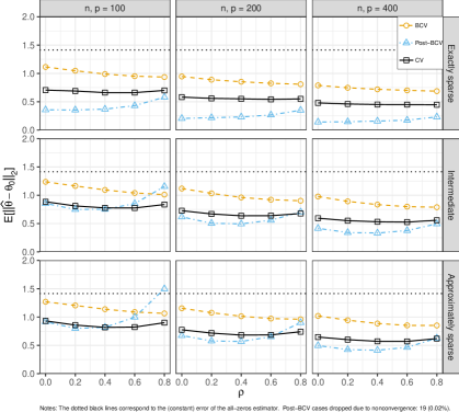
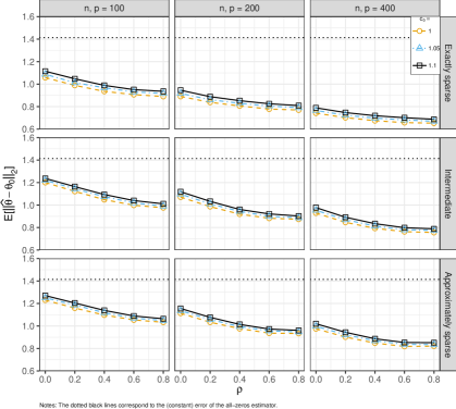
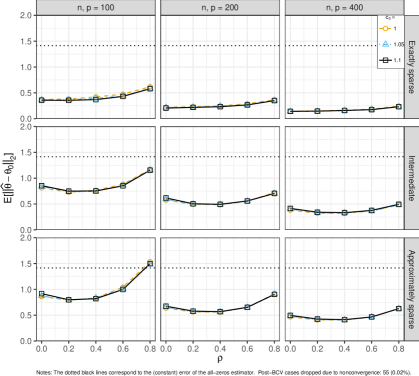
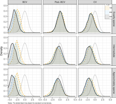
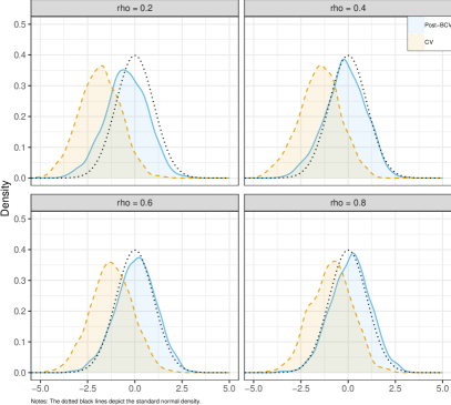
For both estimation and inference purposes, the BCV and Post-BCV estimators resulting from the ad hoc rule perform similarly to those resulting from the rule αn=.1/ln(pn)subscript𝛼𝑛.1𝑝𝑛\alpha_{n}=.1/\ln(p\lor n). The rankings and conclusions of the main text therefore appear robust to the choice of αnsubscript𝛼𝑛\alpha_{n}.

Appendix I Comparison with Existing Penalty Methods

For specific models and loss functions, existing methods for choosing the penalty can be used to estimate 𝜽0subscript𝜽0\bm{\theta}_{0}. One theoretically justifiable method is based on moderate deviation theory for self-normalized sums as detailed in Jing et al. (2003) and de la Pena et al. (2009). Building on various structures (e.g. mean-square projection or Lipschitz loss), data-driven self-normalization is used in both Belloni et al. (2012) and Belloni et al. (2016) for the LASSO and 1subscript1\ell_{1}-penalized logistic regression, respectively. We next compare the performance of our BCV penalty method with the self-normalized penalty methods in each of these papers. Our main finding is that whenever the self-normalized penalty methods work, they provide results which are rather similar to those obtained from our BCV method.

I.1 Comparing with Belloni et al. (2012) Penalty Method

We here consider data-generating processes identical to those in Section 6 except that the outcome is generated as

Yi=𝑿i𝜽0+εi,εi𝑿iN(0,1),i[n],formulae-sequencesubscript𝑌𝑖superscriptsubscript𝑿𝑖topsubscript𝜽0subscript𝜀𝑖formulae-sequencesimilar-toconditionalsubscript𝜀𝑖subscript𝑿𝑖N01𝑖delimited-[]𝑛Y_{i}=\bm{X}_{i}^{\top}\bm{\theta}_{0}+\varepsilon_{i},\quad\varepsilon_{i}\mid\bm{X}_{i}\sim\mathrm{N}(0,1),\quad i\in\left[n\right],

thus implying a linear model with Gaussian errors. Taking m𝑚m to be the (one-half) square loss (1/2)(yt)212superscript𝑦𝑡2(1/2)(y-t)^{2}, the 1subscript1\ell_{1}-ME in (1.2) is the LASSO (Tibshirani, 1996).

Belloni et al. (2012, Algorithm A.1) provides a data-driven penalization scheme allowing for non-Gaussianity, conditionally heteroskedastic errors and regressors measured on different scales. We here compare with a slightly simplified two-step version of their algorithm, presuming that the researchers knows that (i) the regressors are measured on the same scale, and (ii) the errors are conditionally homoskedastic (with variance unknown). These simplifications are only made to ease exposition and reduce the computational burden involved in the comparison.444444We also presume that the researcher knows that the true intercept is zero. Hence, we do not include a constant regressor and penalize all regressor coefficients.

With conditionally homoskedastic errors and equivariant regressors, a two-step version of Belloni et al. (2012, Algorithm A.1) goes as follows:

  1. 1.

    Initial: Calculate an initial penalty level

    λ^α𝚋𝚛𝚝:=c0σ^yΦ1(1α/(2p))n,assignsubscriptsuperscript^𝜆𝚋𝚛𝚝𝛼subscript𝑐0subscript^𝜎𝑦superscriptΦ11𝛼2𝑝𝑛\widehat{\lambda}^{\mathtt{brt}}_{\alpha}:=\frac{c_{0}\widehat{\sigma}_{y}\Phi^{-1}(1-\alpha/(2p))}{\sqrt{n}},

    where σ^y2superscriptsubscript^𝜎𝑦2\widehat{\sigma}_{y}^{2} is the outcome sample variance, and store the residuals ε^i:=Yi𝑿i𝜽^,i[n],formulae-sequenceassignsubscript^𝜀𝑖subscript𝑌𝑖superscriptsubscript𝑿𝑖top^𝜽𝑖delimited-[]𝑛\widehat{\varepsilon}_{i}:=Y_{i}-\bm{X}_{i}^{\top}\widehat{\bm{\theta}},i\in[n], from any LASSO solution 𝜽^Θ^(λ^α𝚋𝚛𝚝)^𝜽^Θsubscriptsuperscript^𝜆𝚋𝚛𝚝𝛼\widehat{\bm{\theta}}\in\widehat{\Theta}(\widehat{\lambda}^{\mathtt{brt}}_{\alpha}).

  2. 2.

    Refined: Calculate a refined penalty level

    λ^α𝚋𝚌𝚌𝚑:=c0σ^εΦ1(1α/(2p))n,assignsubscriptsuperscript^𝜆𝚋𝚌𝚌𝚑𝛼subscript𝑐0subscript^𝜎𝜀superscriptΦ11𝛼2𝑝𝑛\widehat{\lambda}^{\mathtt{bcch}}_{\alpha}:=\frac{c_{0}\widehat{\sigma}_{\varepsilon}\Phi^{-1}(1-\alpha/(2p))}{\sqrt{n}},

    where σ^ε2superscriptsubscript^𝜎𝜀2\widehat{\sigma}_{\varepsilon}^{2} is the residual sample variance {ε^i}i=1nsuperscriptsubscriptsubscript^𝜀𝑖𝑖1𝑛\{\widehat{\varepsilon}_{i}\}_{i=1}^{n}. The Belloni et al. (2012) estimator is then any LASSO solution 𝜽^Θ^(λ^α𝚋𝚌𝚌𝚑)^𝜽^Θsubscriptsuperscript^𝜆𝚋𝚌𝚌𝚑𝛼\widehat{\bm{\theta}}\in\widehat{\Theta}(\widehat{\lambda}^{\mathtt{bcch}}_{\alpha}).

As in Belloni et al. (2012), in the above we use c0=1.1subscript𝑐01.1c_{0}=1.1 and α=αn=.1/ln(np)𝛼subscript𝛼𝑛.1𝑛𝑝\alpha=\alpha_{n}=.1/\ln(n\lor p). Note that the (simplified) initial step here corresponds to the penalty level λ^α𝚋𝚛𝚝subscriptsuperscript^𝜆𝚋𝚛𝚝𝛼\widehat{\lambda}^{\mathtt{brt}}_{\alpha} and resulting estimator suggested in Bickel et al. (2009).

Figure I.1 plots the mean 2subscript2\ell_{2} estimation errors resulting from the BCV, Bickel et al. (2009) (BRT09) and in Belloni et al. (2012) (BCCH12) penalty methods, respectively, considering the sample and problem sizes (n𝑛n and p𝑝p), correlation levels (ρ)𝜌(\rho) and coefficient patterns considered in Section 6 (for the binary probit). The figure shows that BCV performs at least as well as the other methods, However, compared to the here theoretically justifiable BCCH12 method, the BCV improvement is modest.

Figure I.1: Comparing with Belloni et al. (2012) Penalty Method (for LASSO)
Refer to caption

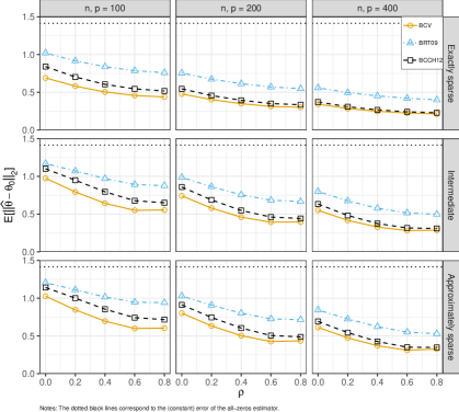
I.2 Comparing with Belloni et al. (2016) Penalty Method

We here consider data-generating processes identical to those in Section 6 except that the outcome is generated as

Yi=𝟏(𝑿i𝜽0+εi>0),εi𝑿iLogistic(0,1),i[n],formulae-sequencesubscript𝑌𝑖1superscriptsubscript𝑿𝑖topsubscript𝜽0subscript𝜀𝑖0formulae-sequencesimilar-toconditionalsubscript𝜀𝑖subscript𝑿𝑖Logistic01𝑖delimited-[]𝑛Y_{i}=\mathbf{1}\left(\bm{X}_{i}^{\top}\bm{\theta}_{0}+\varepsilon_{i}>0\right),\quad\varepsilon_{i}\mid\bm{X}_{i}\sim\mathrm{Logistic}(0,1),\quad i\in\left[n\right],

thus implying a binary logit model as in Example 1. We take m𝑚m to be the negative logit likelihood loss in (2.2).

The notes of Belloni et al. (2016, Table 1) suggest the penalty level

λα,nbcw:=c0Φ1(1α/(2p))2n,assignsubscriptsuperscript𝜆bcw𝛼𝑛subscript𝑐0superscriptΦ11𝛼2𝑝2𝑛\lambda^{\texttt{bcw}}_{\alpha,n}:=\frac{c_{0}\Phi^{-1}(1-\alpha/(2p))}{2\sqrt{n}},

where we continue to use c0=1.1subscript𝑐01.1c_{0}=1.1 and α=αn=.1/ln(np)𝛼subscript𝛼𝑛.1𝑛𝑝\alpha=\alpha_{n}=.1/\ln(n\lor p).454545 See Belloni et al. (2018, Algorithm 3) for details on how to handle regressors measured on different scales. As in Belloni et al. (2016), we (correctly) presume that the regressors are equivariant, and that the true intercept is zero. Hence, we do not include a constant regressor and penalize all regressor coefficients.

Figure I.2 plots the mean 2subscript2\ell_{2} estimation errors resulting from the BCV and Belloni et al. (2016) (BCW16) penalty methods, respectively, considering the sample and problem sizes (n𝑛n and p𝑝p), correlation levels (ρ)𝜌(\rho) and coefficient patterns considered in Section 6 (for the binary probit). The figure shows that BCV performs at least as well as BCW16. However, compared to the here theoretically justifiable BCW16 method, the BCV improvement is again modest.

Figure I.2: Comparing with Belloni et al. (2016) Penalty Method (for 1subscript1\ell_{1}-Penalized Logit)
Refer to caption