High-altitude polar NM with the new DAQ system as a tool to study details of the cosmic-ray induced nucleonic cascade
Abstract
A neutron monitor (NM) is, since the 1950s, a standard ground-based detector whose count rate reflects cosmic-ray variability. The worldwide network of NMs forms a rough spectrometer for cosmic rays. Recently, a brand-new data acquisition (DAQ) system has been installed on the DOMC and DOMB NMs, located at the Concordia research station on the Central Antarctic plateau. The new DAQ system digitizes, at a 2-MHz sampling rate, and records all individual pulses corresponding to secondary particles in the detector. An analysis of the pulse characteristics (viz. shape, magnitude, duration, waiting time) has been performed, and several clearly distinguishable branches were identified: (A) corresponding to signal from individual secondary neutrons; (B) representing the detector’s noise; (C) double pulses corresponding to the shortly separated nucleons of the same atmospheric cascades; (D) very-high multiple pulses which are likely caused by atmospheric muons; and (E) double pulses potentially caused by contamination of the neighbouring detector. An analysis of the waiting time distributions has revealed two clearly distinguishable peaks: peak (I) at about 1 msec being related to the intra-cascade diffusion and thermalisation of secondary atmospheric neutrons; and peak (II) at 30 – 1000 msec corresponding to individual atmospheric cascades. This opens a new possibility to study spectra of cosmic-ray particles in a single location as well as details of the cosmic-ray induced atmospheric cascades, using the same dataset.
JGR: Space Physics
Space Physics and Astronomy Research Unit, University of Oulu, Finland Sodankylä Geophysical Observatory, University of Oulu, Finland Ioffe Physical-Technical Institute RAS, St. Petersburg, Russia Center for Space Research, North-West University, Potchefstroom, South Africa
Ilya Usoskinilya.usoskin@oulu.fi
New data-acquisition (DAQ) systems, digitizing all pulses at a 2-MHz sampling rate, is installed and tested at DOMC/DOMB neutron monitors.
Several branches are identified in the pulse parameters, corresponding to different processes.
The new DAQ system allows studying inter-cascade, intra-cascade and instrumental response separately from the same dataset.
1 Introduction
A neutron monitor (NM) is a standard ground-based detector to monitor cosmic-ray variability in the near-Earth environment [Shea \BBA Smart (\APACyear2000), Vainio \BOthers. (\APACyear2009), Usoskin \BOthers. (\APACyear2017)]. The design of the NM was developed in 1957 (called IGY — International Geophysical Year) and improved in 1964 (called NM64), and since then it is used as a standard detector [Simpson (\APACyear1958), Simpson (\APACyear2000), Stoker (\APACyear2009)]. NMs record primarily the secondary nucleonic component (mostly neutrons) of the cosmic-ray induced atmospheric cascade with a small fraction of counts caused by muons. Its count rate is defined by the flux of primary (impinging on the top of the atmosphere) cosmic rays, as a combination of the cosmic-ray energy spectrum, detector’s yield function and geomagnetic rigidity cutoff [Clem \BBA Dorman (\APACyear2000), Mishev \BOthers. (\APACyear2020)]. The NM is an energy-integrating detector, with the effective energy ranging from about 12 GeV for polar NMs to 35 GeV for equatorial ones [Asvestari \BOthers. (\APACyear2017)]. The sensitivity of NMs to low-energy cosmic rays is highest in polar regions (low or no geomagnetic shielding) and high altitudes (lower atmospheric shielding) and decreases towards equatorial latitudes. The worldwide network of NMs can act as a giant spectrometer able to roughly estimate the spectrum of both galactic cosmic rays [<]e.g.,¿[]dorman04 and relativistic solar protons [<]e.g.,¿[]duggal79,mishev14. Along with the count rate, the multiplicity of NM counts (the average number of pulses within a short time interval) is sometimes studied [Dorman (\APACyear2004), Balabin \BOthers. (\APACyear2011)] as a rough index of the spectral hardness of cosmic rays. Sometimes NM are accompanied by separate muon detectors to measure high-energy cosmic rays.
This work is focused at two mini-NMs, DOMC and DOMB, located at the Concordia Antarctic Research station on top of Dome C, Central Antarctic plateau (75∘06’S, 123∘23’E, 3233 m above sea level) [Poluianov \BOthers. (\APACyear2015)]. They are ones of the most sensitive NMs to lower energy cosmic rays (including solar energetic particles) thanks to the highly elevated polar location. Each NM has one BF3-filled detector surrounded by reflecting and moderating layers of polyethylene. In addition, DOMC has a layer of lead serving as a neutron producer to increase the detector efficiency. DOMB has no lead layer and therefore has lower efficiency than DOMC, but is more sensitive to low-energy secondary cosmic-ray particles [Vashenyuk \BOthers. (\APACyear2007)]. Recently, those instruments got a major upgrade of the data-acquisition system (DAQ). Traditionally, a standard NM records only the count rate of cosmic rays, while the new electronics of DOMC and DOMB digitizes individual detector pulses with a sub-microsecond precision [<]2-MHz sampling rate, see¿[]strauss20. In this work, we study new opportunities provided by the DAQ upgrade, by using the statistic of recorded pulses and show that it allows one to study details of the cosmic-ray induced atmospheric cascade with instruments like DOMB and DOMC.
2 DOMC/DOMB DAQ electronic system
The new DAQ system is built with a single-board computer Raspberry Pi 3B and easily replaceable modules responsible for the operation of different subsystems (high voltage power supply, pre-amplifier and detector signal processor, temperature-pressure-humidity sensors and others) – see full details in \citeAstrauss20.
Pulse signals coming from the detector are amplified and digitized by a signal registration board. It has a dedicated microcontroller PIC32 and built-in 10-bit analogue-to-digital converter (ADC) with the reference voltage set at 3.3 V. Each pulse is sampled at the frequency of 2 MHz (viz. 0.5 sec), and the information about its magnitude time profile is stored in a buffer of the board. The central computer has software-defined discriminators in pulse’s magnitude and length. If a pulse in the buffer matches both criteria, it gets recorded in a data file by the central computer. The files are compressed and sent to the data server of Oulu cosmic ray station for further import to databases cosmicrays.oulu.fi and nmdb.eu.
DOMC and DOMB have the following default thresholds for registered pulses: the magnitude discriminator at 0.2 V and the minimum pulse length of five sample points (2.5 sec). All pulses failing to meet these criteria are ignored by the DAQ system. Since each pulse with the magnitude exceeding 0.2 V and longer than 2 sec is digitized, a higher-value thresholds can be applied electronically in the off-line analysis.
Analyses of the pulse shapes and statistics are presented in the subsequent sections.
3 Analysis of pulse shapes
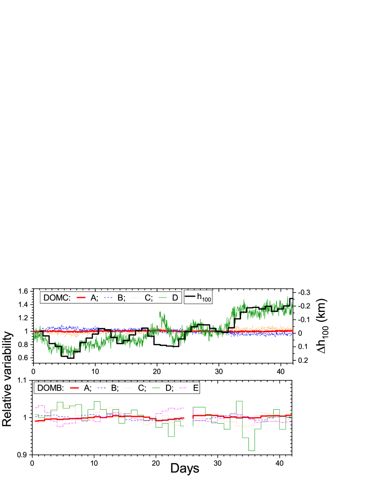
Here, we used data from DOMC for 01-Jan through 31-May-2020 (about pulses recorded), and from DOMB for 13-Aug through 31-Oct-2019 ( individual pulses recorded). These periods correspond to very quiet solar conditions (solar cycle minimum) with relatively low heliospheric modulation and high intensity of galactic cosmic rays (GCR). There were no solar particle events or other notable transients during the studied period. The period of January through May 2020 corresponded to a transition from polar-day (around-a-clock insolation) to polar-night (no sunlight) conditions and formation of the polar vortex. The period of August – October 2019 was characterized by very stable and cold weather with a stable polar vortex. An example of temporal variability of the pressure-corrected count rates in different branches (see below) are shown in Figure 3 for the first 42 days of each analyzed period. For correction, the following barometric coefficients were used: -0.769 %/hPa for DOMC and -0.754 %/hPa for DOMB (the reference pressure level 650 hPa) as defined during the operation of the detectors (see, e.g., metadata in http://cosmicrays.oulu.fi). One can see that the overall pressure-corrected count-rate vary within % only, but the variability in other branches is greater as described below.
For the analysis, we used the following pulse parameters: magnitude (the maximum voltage); length (the duration, in sec of the signal being above the selected threshold); the -folding decay time of the exponential decline of the pulse voltage after the maximum, and the waiting time between onsets of subsequent pulses (in sec).
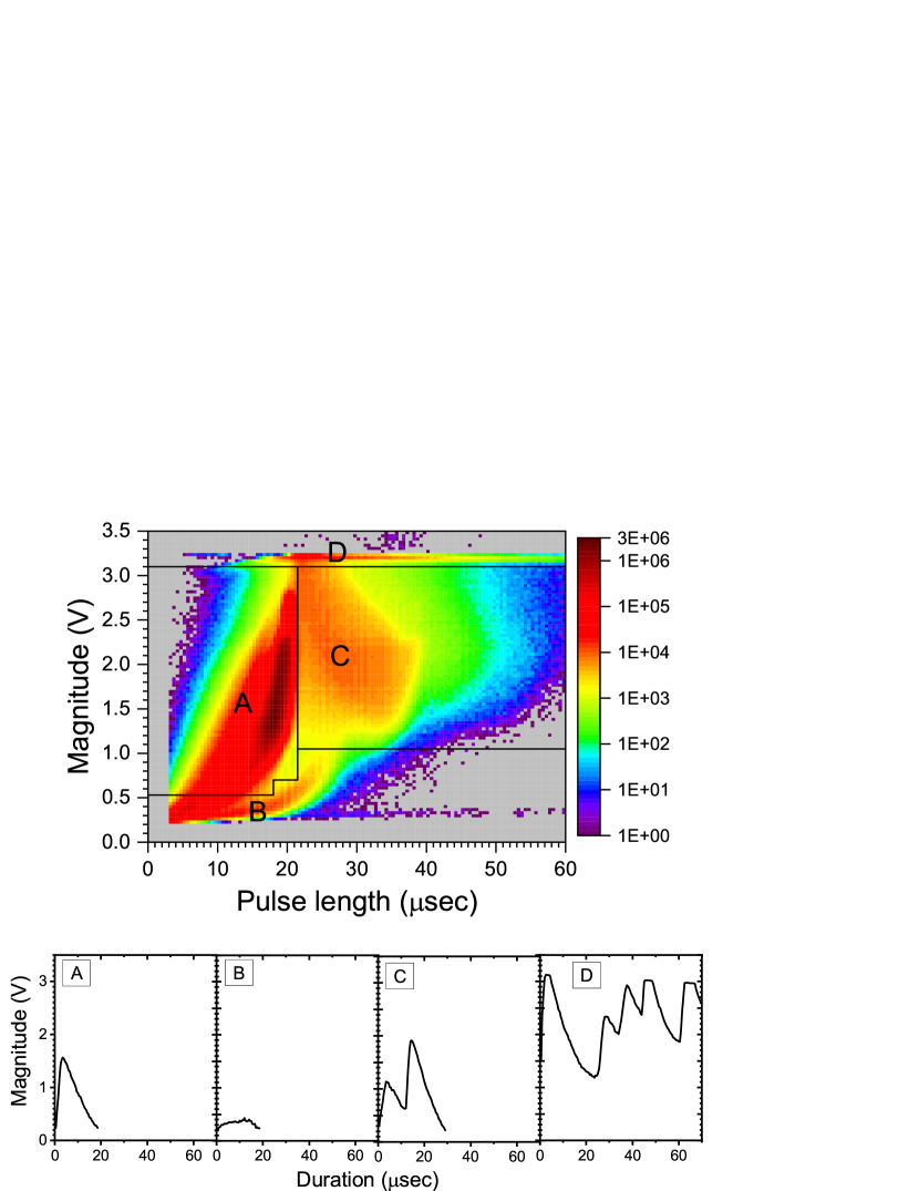
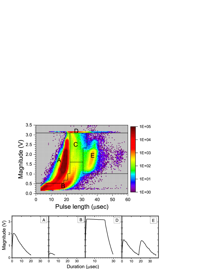
First, we analyzed the relation between the magnitude and the length of all individual pulses. These distributions are presented in Figures 1 and 2, respectively for the DOMC and DOMB NMs [<]cf. Figure 4 in¿[]strauss20. Several clearly distinguished branches can be identified (see statistic in Table 1):
3.1 Branch A: Normal pulses
The main branch contains the majority (90 %) of the pulses. It consists of single, well-defined pulses with a fast rise (a few sec) followed by an exponential decline with the -folding decay time sec, defined by the pre-amplifier’s circuit (relaxation of a capacitor). Samples of typical pulses in this branch can be observed in Figures 1A and 2A for DOMC and DOMB NMs, respectively. The magnitude takes the entire range up to 3 V, and duration 5 – 20 sec, with a tendency that higher pulses are slightly longer, as they decay to the detection threshold level longer. However, since low pulses (0.5 V) are mixed with the branch B (noise), we consider normal pulses as those with 0.5 V. The time variability of the count rate in this branch is perfectly corrected for pressure (the formal Pearson correlation between the daily count rate and the pressure is -0.02) and remains stable within % in both DOMC and DOMB. This is the clear signal part which forms the main fraction (%) of the count rate, while the remaining 8 – 9 % of pulses need more discussion.
3.2 Branch B: Noise
This branch contains very low ( V) pulses without any clear shape (see Figures 1B and 2B). The positive correlation between and is expected for the same reason as for branch A. These pulses are likely related to electronic noise. This component comprises 5 – 7 % of the total number of pulses but can be reduced to 1%, thus improving the signal-to-noise ratio from 15 to 90 by increasing the magnitude threshold level up to 0.5 – 0.6 V. Since the short-length (12 sec) pulses are contributed also from branch A (normal pulses), the percentage above is a conservative upper limit. This branch depicts hardly any time variability as expected for the noise, but after nominal pressure correction (Figure 3) it appears ’over-corrected’ and depicts slight variability in phase with the pressure (r=0.290.15, value =).
3.3 Branch C: Contribution of atmospheric cascade
This branch consists of moderately high ( V) and longer (20 – 35 sec) pulses. They are typically double peaks (Figure 1C) where the second peak starts before the first one drops below the detection level. The negative correlation between the magnitude and the length is understandable, as the second pulse starts over non-zero background. The separation between the pulses is from 5 – 20 sec. The sub-pulses are totally consistent with the pulses in branch A in duration and decay time (sec). This branch is clear in DOMC data, comprising about 3% of all pulses, but is hardly visible (only 0.24 %) in the DOMB dataset, implying that is caused by a nucleonic component. The time separation between the subpulses (sec) is much longer than the characteristic time (expected to be of the order of several nanoseconds) of a cascade within the detector itself, including lead producer, but shorter than the full development of the atmospheric cascades (see Section 4). It is likely related to a tail of the WTD for the atmospheric cascade development (Section 4), when the time separation between secondary nucleons of the same cascade appear shorter than the single pulse length of 20 sec. Such pulses are registered as long ones composed of two partly overlapping pulses and form branch C. Contributions of nucleons with longer time separation make single pulses associated to branch A. The count-rate variability in this branch (Figure 3) still depicts dependence (under-correction) on pressure after the nominal pressure correction (r=-0.260.16, =), implying a stronger dependence on pressure than that for branch A. We note that the standard NM64 electronic setup with the dead-time (20 sec) makes this branch indistinguishable from branch A.
3.4 Branch D: Possible contribution of muons
This branch is characterized by very high magnitude ( V, viz. near the upper bound of ADC) and long duration of pulses. Most numerous here are saturated pulses (Figure 2D) but there are also very long pulses, up to 110 sec in length, that include a sequence of short but very high sub-pulses following each other by several sec (Figure 1D). The saturated pulses would require, if fitted with a ‘standard’ pulse shape (Fig. 1A), a very high magnitude of up to 30 V, viz. a factor of 10 greater than normal pulses. Multiple pulses may contain up to 10 short sub-pulses, also implying an enhanced yield. This points to a different type of process producing pulses in branch D. The most plausible candidate is the process of direct multiple-ion production by a cascade muon in BF3 gas inside the NM proportional counter [Knoll (\APACyear2010), Siciliano \BBA Kouzes (\APACyear2012)]. This can ignite multiple, nearly simultaneous electromagnetic avalanches inside the counter, leading to more ‘energetic’ recorded pulses (voltage exceeding the upper limit and/or multiple overlapping pusles – see Figures 2D and 1D, respectively). This process has not been considered nor properly modelled for NMs, where its contribution is small, in contrast to the usually considered muon contribution to NM counts, viz. muon-induced production of neutrons in the lead producer [Clem \BBA Dorman (\APACyear2000)] with subsequent detection in the counter [Maurin \BOthers. (\APACyear2015), Mangeard \BOthers. (\APACyear2016)]. Such muon-induced neutrons are detected in a usual way and cannot be distinguished from the signal of the hadronic component. Accordingly, they appear in branch A and cannot contribute to branch D. Therefore, we can speculate that the branch D is likely related to non-hadronic particles producing abnormally energetic pulses via direct ionization of the filling gas. A more detailed study of this process is planned for the future.
Count-rate in this branch (Figure 3) depicts strong variability: 25% for DOMC and 5% for DOMB, which can be explained by a strong change in the atmospheric density profile and by a stable vortex conditions, during the two analyzed periods, respectively. For comparison, we shown in Figure 3A the temporal variability, for the same period, of the anomaly of the geopotential height of the (100 hPa) atmospheric level, which roughly corresponds to the mean height of the muon production and affects the muon flux near ground. The branch-D count rate co-varies in sync with (=-0.84, -value ), and the magnitude of the muon-flux variability is consistent with the km using the measured spectrum of muons [Boezio \BOthers. (\APACyear2003)] at a 100-hPa level and relativistic time dilation. This confirms the muon origin of this branch since no other source can reliably explain it. We emphasize that this effect is strong for the high altitude of DOMC location but fades towards lower heights (because of the higher energy of muons that can reach lower altitudes) and accounts for only 5% at sea level of 1013 hPa. Thus, the NM with a high magnitude threshold ( V) can operate as a low-efficiency muon detector.
3.5 Branch E: Possible contamination from DOMC
There is a branch with pulses of a normal magnitude ( between 1 – 2.5 V) and double length (35 – 40 sec) clearly visible for DOMB NM (Figure 2). This branch contains 0.28 % of all pulses and is composed of double pulses (Figure 2E) separated by 10 – 20 sec. Interestingly, this branch is not distinguishable in DOMC data (Figure 1). We do not have a clear understanding of the origin of this branch but may speculate that it is possible contamination from multiple neutrons produced by the lead producer of the neighbouring DOMC detector. Because of the diffusive propagation, the neutrons may arrive to DOMB at slightly different times. The detectors are located about 1 meter apart of each other, leading to a 20-sec traversing time for one meter of air and several g/cm2 of the moderator/reflector layers. We note that if the two pulses are separated by more than 25 sec so that the voltage drops below the discriminator’s level, the pulses are counted as two separate ones. An insignificant hint on triple pulses can be observed in Figure 2 at 50 sec. We note that 20 sec is known as electronic ‘dead-time’ of a standard NM [Hatton \BBA Carimichael (\APACyear1964)]. Nothing conclusive can be seen in the time variability of this branch, because of the low statistics (about 1 count per minute).
This branch could be potentially caused also by noise in the pre-amplifier’s electric circuit, by producing an ‘echo’ of the signal with a delay time of 20 sec, viz. double – triple characteristic time of the circuit (8 sec). However, this is unlikely since such echoing was not observed during electronic tests of the DAQ board.
| Branch | percentage | Possible origin | |
|---|---|---|---|
| DOMC | DOMB | ||
| A | 90.98 | 91.49 | Main branch: single pulses |
| B | 5.20† | 7.84† | Noise |
| C | 3.15 | 0.23 | Multiple pulses from the same atmospheric cascade |
| D | 0.68 | 0.16 | Possible muon contribution |
| E | – | 0.28 | Possible contamination from the neighbouring detector |
† the percentage is a conservative upper bound as this branch includes also pulses from branch A.
4 Waiting time distribution
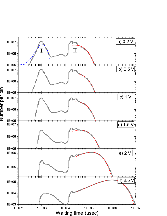
Next, we have analyzed the waiting-time distribution (WTD) of recorded pulses. We define the waiting time as the time interval between the onsets of consecutive pulses recorded by the DAQ system of a NM. Since the length of individual pulses can reach 100 sec (Figures 1 and 2), we analyse the WTD for sec. The observed WTDs are plotted, as logarithmically-binned histograms in Figures 4 and 5, respectively for DOMC and DOMB NMs, for different values of the magnitude threshold so that . The distributions for different values of have a similar shape with two clearly separated peaks: one (called peak ) at msec, the other (peak ) located between 30 msec and 10 sec depending on the value of and the detector type.
4.1 Peak I: In the atmospheric cascade
The first WTD peak (peak ) is located at msec. Its location is very stable and does not depend on the values, nor on the detector type. On the other hand, the peak broadens for higher threshold values extending its tail to longer waiting times, up to several milliseconds. The contribution of this peak to the total count rate varies from about 35% (no additional threshold) down to 2.5% ( V) for DOMC NM, and from 7% down to 0.1% for the DOMB NM, respectively. We note that, while the bulk of secondary protons, muons, and electromagnetic components of the cascade arrive to a detector as a relatively thin front, secondary neutrons diffuse in the atmosphere, leading to a wide spread in time and lateral distribution compared to other secondaries [Grieder (\APACyear2011)].
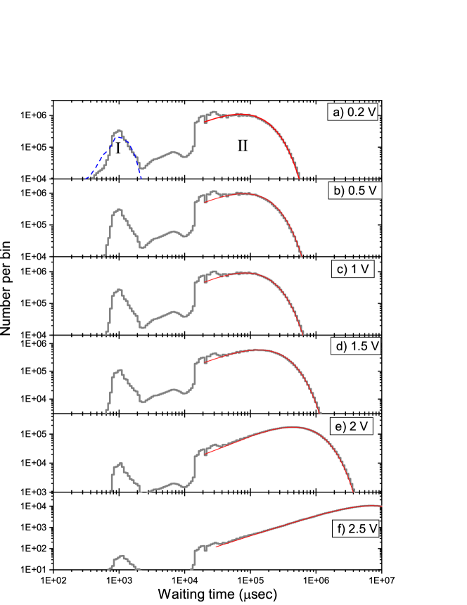
In order to check that, we performed a numerical simulation of the development of the atmospheric cascade using the Monte-Carlo simulation toolbox Geant4 v.10.6.0 [Agostinelli \BOthers. (\APACyear2003), Allison \BOthers. (\APACyear2006)] with the physics list QGSP_BIC_HP (Quark-Gluon String model, Geant4 Binary Cascade model, High-Precision neutron package) [Geant4 collaboration (\APACyear2020)]. We simulated atmospheric cascades initiated by incident protons with the kinetic energy of 10 GeV impinging vertically on the top of the atmosphere. We note that this energy corresponds to the effective energy of a polar NM to GCR [Kudela \BOthers. (\APACyear2000), Asvestari \BOthers. (\APACyear2017)] and thus roughly represents the relation between the NM count rate and CR variability. During the simulations, we traced secondary neutrons and recorded their crossing of the reference level of 650 g/cm2 where the DOMC/DOMB NMs are located. For each neutron crossing, the neutron’s energy, location with respect to the cascade axis and the time since the first interaction were recorded for further analysis. Neutrons were found to spread as far as 6 km from the cascade axis [<]see also¿[]paschalis11 with the delay of up to 80 milliseconds. Next, we built a logarithmically-binned histogram of the WTD between arrivals of epithermal neutrons ( keV) with spatial separation less than 1 meter, from the same atmospheric cascade, as shown by the blue dashed curve in Figures 4a and 5a. The distribution reasonably well matches both the location and width of peak I. The height of the distribution was scaled up to match the observed WTD, while keeping the shape and location of the peak. Similar results can be obtained for other energies of the primary particle since the 1-msec time is caused by diffusion and thermalization of secondary neutrons from 1 MeV (evaporation peak) to 10 keV energy, and not by the development of a cascade per se.
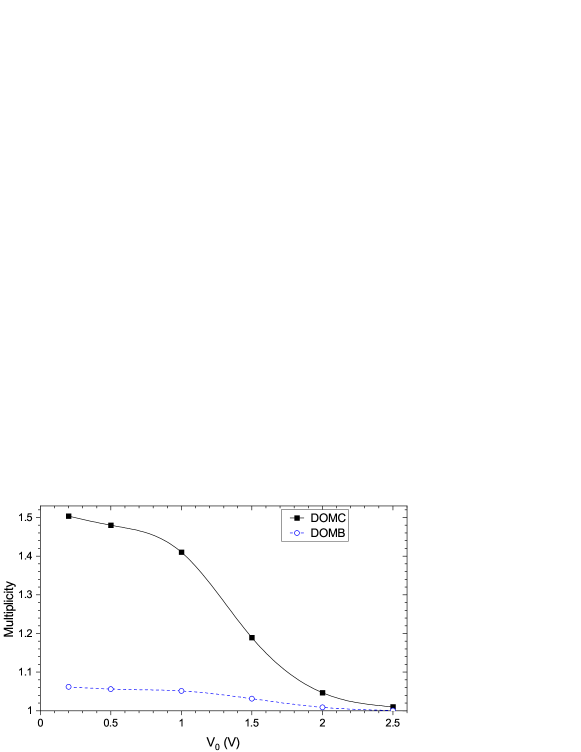
Accordingly, WTD peak I can be reliably associated with the neutron diffusion and thermalization within atmospheric cascades, and the time of about one millisecond is a typical time-scale for such a process. These pulses generally contribute to the well-known multiplicity of NM counts [Debrunner \BBA Walther (\APACyear1968), Balabin \BOthers. (\APACyear2011), Mangeard \BOthers. (\APACyear2016), Ruffolo \BOthers. (\APACyear2016)], viz. multiple correlated pulses within the NM count rate. The mean multiplicity of the NM count rate for different threshold values is shown in Figure 6. It is calculated as the ratio of the total number of counts for each NM to that in peak II, viz. the number of individual cascades. The obtained values for the multiplicity (1.5 and 1.06 for for DOMC and DOMB, respectively) are slightly higher than those measured at sea level [Hatton \BBA Carimichael (\APACyear1964)] but lower than that for an air-borne NM [Kent \BOthers. (\APACyear1968)].
4.2 Peak II: Individual atmospheric cascades
The other peak (called peak II) is quite broad and corresponds to the waiting times from about 20 msec to several seconds. The distribution is slightly distorted between 10 and 40 msec, probably due to interference with the power-line frequency (50 Hz). The peak has a well-defined smooth shape, and its location depends on the detector (DOMB and DOMC) and the value of the threshold (Figures 4 and 5). This peak in WTD corresponds to individual atmospheric cascades caused by the primary cosmic-ray particles. In order to illustrate this, we have also plotted (as red curves) the analytically expected WTD for randomly occurring independent pulses with the occurrence probability defined by the observed count rate of a given NM (DOMC or DOMB) for a given value . WTD of independently occurring events with the occurrence probability is expected to be exponential with the characteristic decay time , which takes for a logarithmically binned histogram the shape shown by the red curves. One can see that the analytical WTD perfectly describes the observed peak II for different values of and for both DOMC and DOMB, confirming its relation to the individual atmospheric cascades.
The observed WTD is consistent with the recently introduced delay time–geometry correction factor for the NM yield function, details are given elsewhere [Mishev \BOthers. (\APACyear2013), Mishev \BOthers. (\APACyear2020)].
5 Discussion and conclusions
The new DAQ system of neutron monitors makes it possible to study different processes induced by cosmic rays in the atmosphere and the detector itself. In Sections 3 and 4 we have analyzed different pulse parameters and waiting times. Somewhat similar analyses were made also earlier [Hatton \BBA Tomlinson (\APACyear1968)] using oscilloscopes and were based on small statistic. The new DAQ system allows continuous analysis of the pulses, e.g., the statistic shown here includes and individual pulses for the DOMC and DOMB, respectively, for illustration, but it can be much greater. Thanks to the fully digitized pulses, the same dataset recorded by the new DAQ system allows studying different processes separately.
Individual atmospheric cascades can be studied as pulses separated by more than two milliseconds, which is close to the standard NM detection mode with the dead-time of 1.2 msec [Hatton \BBA Carimichael (\APACyear1964)]. It is important that, in contrast to the standard NM64 DAQ system with the fixed “dead-time”, waiting time between pulses can be now performed by software data-processing.
Development of the atmospheric cascade can be studied using pulses with waiting times between 0.3 and 3 msec. This is not usually done in the NM data analysis directly but rather via the multiplicity (or ‘leader-fraction’) analyses. With the new DAQ system, one can study details of the cascade development for each cascade individually, including also the multiplicity.
Development of the atmospheric cascade in the vicinity of the detector can be studied using the pulse-shape analysis, in particular, in branches C and D in Figures 1 and 2. In particular, with the high magnitude threshold, the NM can operate as a low-efficiency muon detector. We are not aware of any similar analysis done previously. Moreover, a detailed analysis of branches C and D allows one to discriminate hadrons from muons, and hence to use an NM in a regime of muon detector, using the same dataset.
The noise is shown to form a well-separated branch, being characterized by the low pulse magnitude. Accordingly, by selecting the discriminator threshold to the value of 0.5 – 0.6 V (the default is 0.2 V) one can cut off the noise effectively without a significant reduction of regular pulses. Placing the threshold to 0.5 V eliminates about 90% of the noise and only a few percent of normal pulses, thus increasing the signal-to-noise ratio by an order of magnitude.
The standard NM is an energy-integrating detector and cannot measure the energy spectrum of cosmic rays. Combining NM with different geomagnetic cutoff rigidities to the worldwide network makes them a very rough spectrometer [Moraal \BOthers. (\APACyear2000)]. It works reasonably well for GCR [Caballero-Lopez \BBA Moraal (\APACyear2012)] but cannot be directly applied to a study of solar energetic particles because of the possible anisotropy which can be large during impulsive (phase of) events [<]e.g.,¿[]mishev14. Data from different NMs cannot be compared directly without a complicated analysis of magnetospheric transport of charged particles [<]e.g.,¿[]smart00. The use of a pair of standard and bare NMs in the same location (e.g. at the South Pole, SANAE or Dome C stations) provides a rough measure of the hardness of the cosmic-ray spectrum [Caballero-Lopez \BBA Moraal (\APACyear2016), Nuntiyakul \BOthers. (\APACyear2018)], based on the ratio of their count rates. Here we propose that the use of different -values in the new DAQ-system dataset may provide an estimate of the cosmic-ray spectrum. Specifically, a muon-related branch of the pulses can be separated, providing muon counts in the same detector. Fine analysis of relatively weak ground-level solar particle events is often very limited due to the shortage of information about the energy spectrum since such events are seen only by a few high-altitude polar NMs with no significant response from sea-level and non-polar instruments [Mishev \BOthers. (\APACyear2017)]. In such a case, any spectral information is very crucial and any new addition significantly increases the quality of the analysis. Varying the value of , one can obtain several spectral points. In particular, the measured waiting time and magnitude distributions of pulses could serve for that purpose. In an ideal case, a strong SEP event, such as the GLE#69 of 20-Jan-2005, could be used to ‘calibrate’ the detector, but such events occur very seldom. Alternatively, this possibility can be explored quantitatively with a full simulation of the detector-and-atmosphere response to the primary particles. This is doable with the modern Monte-Carlo simulation techniques, but is beyond the framework of this paper and left for forthcoming work.
In summary:
-
1.
A new DAQ system has been installed on DOMC and DOMB NMs that has gathered a large amount of fully digitized, at a sub-sec sampling rate, individual pulses.
-
2.
An analysis of the data has demonstrated clustering of pulses to several branches: (A) the main branch representing secondary neutrons; (B) detector’s electronic noise; (C) double pulses caused by shortly separated pulses of the same atmospheric cascade; (D) multiple pulses likely related to atmospheric muons; (E) possible contamination of DOMB detector by neutrons scattered from the neighbouring DOMC detector.
-
3.
An analysis of the waiting time distributions has revealed two clearly distinguishable peaks: peaks I at about 1 msec related to the intra-cascade diffusion and thermalisation of secondary atmospheric neutrons; and peak II (30 – 1000 msec) corresponding to individual atmospheric cascades.
-
4.
It is shown that a NM with the new DAQ system can provide also data on muon flux, using the same dataset.
This opens a new possibility to study spectra of cosmic-ray particles in a single location and details of cosmic-ray induced atmospheric cascades.
Acknowledgements.
We are grateful to the personnel of Concordia station hosting the DOMC/DOMB instrumentation. Operation of DOMC/DOMB NMs is possible thanks to the hospitality of the Italian polar programme PNRA (via the LTCPAA PNRA 2015/AC3 and the BSRN PNRA OSS-06 projects) and the French Polar Institute IPEV. It is supported by the Academy of Finland (projects CRIPA-X No. 304435, ESPERA No. 321882, QUASARE 330063, HEAIM-2 330427), and Finnish Antarctic Research Program (FINNARP). DOMC/DOMB NM data can be obtained from http://cosmicrays.oulu.fi, courtesy of the Sodankylä Geophysical Observatory.References
- Agostinelli \BOthers. (\APACyear2003) \APACinsertmetastaragostinelli03{APACrefauthors}Agostinelli, S., Allison, J., Amako, K., Apostolakis, J., Araujo, H., Arce, P.\BDBLZschiesche, D. \APACrefYearMonthDay2003. \BBOQ\APACrefatitleGeant4-a simulation toolkit Geant4-a simulation toolkit.\BBCQ \APACjournalVolNumPagesNucl Instr. Meth. Phys. Res. A506250-303. \PrintBackRefs\CurrentBib
- Allison \BOthers. (\APACyear2006) \APACinsertmetastarallison06{APACrefauthors}Allison, J., Amako, K., Apostolakis, J., Araujo, H., Arce Dubois, P., Asai, M.\BDBLYoshida, H. \APACrefYearMonthDay2006. \BBOQ\APACrefatitleGeant4 developments and applications Geant4 developments and applications.\BBCQ \APACjournalVolNumPagesIEEE Transact. Nucl. Sci.53270-278. {APACrefDOI} 10.1109/TNS.2006.869826 \PrintBackRefs\CurrentBib
- Asvestari \BOthers. (\APACyear2017) \APACinsertmetastarasvestari_JGR_17{APACrefauthors}Asvestari, E., Gil, A., Kovaltsov, G\BPBIA.\BCBL \BBA Usoskin, I\BPBIG. \APACrefYearMonthDay2017. \BBOQ\APACrefatitleNeutron Monitors and Cosmogenic Isotopes as Cosmic Ray Energy-Integration Detectors: Effective Yield Functions, Effective Energy, and Its Dependence on the Local Interstellar Spectrum Neutron Monitors and Cosmogenic Isotopes as Cosmic Ray Energy-Integration Detectors: Effective Yield Functions, Effective Energy, and Its Dependence on the Local Interstellar Spectrum.\BBCQ \APACjournalVolNumPagesJ. Geophys. Res. (Space Phys.)1229790-9802. {APACrefDOI} 10.1002/2017JA024469 \PrintBackRefs\CurrentBib
- Balabin \BOthers. (\APACyear2011) \APACinsertmetastarbalabin11{APACrefauthors}Balabin, Y., Gvozdevsk, B\BPBIB., Maurchev, E\BPBIA., Vashenyuk, E\BPBIV.\BCBL \BBA Dzhappuev, D\BPBID. \APACrefYearMonthDay2011. \BBOQ\APACrefatitleFine structure of neutron multiplicity on neutron monitors Fine structure of neutron multiplicity on neutron monitors.\BBCQ \APACjournalVolNumPagesAstrophys. Space Sci. Trans.73283-286. {APACrefDOI} 10.5194/astra-7-283-2011 \PrintBackRefs\CurrentBib
- Boezio \BOthers. (\APACyear2003) \APACinsertmetastarboezio_mu03{APACrefauthors}Boezio, M., Bonvicini, V., Schiavon, P., Vacchi, A., Zampa, N., Bergström, D.\BDBLStochaj, S\BPBIJ. \APACrefYearMonthDay2003. \BBOQ\APACrefatitleEnergy spectra of atmospheric muons measured with the CAPRICE98 balloon experiment Energy spectra of atmospheric muons measured with the CAPRICE98 balloon experiment.\BBCQ \APACjournalVolNumPagesPhys. Rev. D677072003. {APACrefDOI} 10.1103/PhysRevD.67.072003 \PrintBackRefs\CurrentBib
- Caballero-Lopez \BBA Moraal (\APACyear2016) \APACinsertmetastarcaballero16{APACrefauthors}Caballero-Lopez, R\BPBIA.\BCBT \BBA Moraal, H. \APACrefYearMonthDay2016. \BBOQ\APACrefatitleSpectral index of solar cosmic-ray flux from the analysis of ground-level enhancements Spectral index of solar cosmic-ray flux from the analysis of ground-level enhancements.\BBCQ \APACjournalVolNumPagesAdv. Space Res.5761314-1318. {APACrefDOI} 10.1016/j.asr.2015.08.019 \PrintBackRefs\CurrentBib
- Caballero-Lopez \BBA Moraal (\APACyear2012) \APACinsertmetastarcaballero12{APACrefauthors}Caballero-Lopez, R.\BCBT \BBA Moraal, H. \APACrefYearMonthDay2012. \BBOQ\APACrefatitleCosmic-Ray Yield and Response Functions in the Atmosphere Cosmic-ray yield and response functions in the atmosphere.\BBCQ \APACjournalVolNumPagesJ. Geophys. Res.117A12103. {APACrefDOI} 10.1029/2012JA017794 \PrintBackRefs\CurrentBib
- Clem \BBA Dorman (\APACyear2000) \APACinsertmetastarclem00{APACrefauthors}Clem, J.\BCBT \BBA Dorman, L. \APACrefYearMonthDay2000. \BBOQ\APACrefatitleNeutron Monitor Response Functions Neutron monitor response functions.\BBCQ \APACjournalVolNumPagesSpace Sci. Rev.93335–359. {APACrefDOI} 10.1023/A:1026508915269 \PrintBackRefs\CurrentBib
- Debrunner \BBA Walther (\APACyear1968) \APACinsertmetastardebrunner68a{APACrefauthors}Debrunner, H.\BCBT \BBA Walther, U. \APACrefYearMonthDay1968. \BBOQ\APACrefatitleMultiplicity measurements on the IGY neutron monitor at Jungfraujoch Multiplicity measurements on the IGY neutron monitor at Jungfraujoch.\BBCQ \APACjournalVolNumPagesCanadian J. Phys. Suppl.461140. {APACrefDOI} 10.1139/p68-439 \PrintBackRefs\CurrentBib
- Dorman (\APACyear2004) \APACinsertmetastardorman04{APACrefauthors}Dorman, L. \APACrefYear2004. \APACrefbtitleCosmic Rays in the Earth’s Atmosphere and Underground Cosmic rays in the earth’s atmosphere and underground. \APACaddressPublisherDordrechtKluwer Academic Publishers. \PrintBackRefs\CurrentBib
- Duggal (\APACyear1979) \APACinsertmetastarduggal79{APACrefauthors}Duggal, S\BPBIP. \APACrefYearMonthDay1979. \BBOQ\APACrefatitleRelativistic solar cosmic rays Relativistic solar cosmic rays.\BBCQ \APACjournalVolNumPagesRev. Geophys. Space Physics171021-1058. {APACrefDOI} 10.1029/RG017i005p01021 \PrintBackRefs\CurrentBib
- Geant4 collaboration (\APACyear2020) \APACinsertmetastarGeant4-Phys2020{APACrefauthors}Geant4 collaboration. \APACrefYearMonthDay2020. \BBOQ\APACrefatitlePhysics reference manual (version Geant4 10.6.0) Physics reference manual (version Geant4 10.6.0)\BBCQ [\bibcomputersoftwaremanual]. \APACrefnoteavailable from https://geant4.web.cern.ch/ support \PrintBackRefs\CurrentBib
- Grieder (\APACyear2011) \APACinsertmetastargrieder11{APACrefauthors}Grieder, P. \APACrefYear2011. \APACrefbtitleExtensive Air Showers: High Energy Phenomena and Astrophysical Aspects Extensive Air Showers: High Energy Phenomena and Astrophysical Aspects. \APACaddressPublisherNYSpringer. \PrintBackRefs\CurrentBib
- Hatton \BBA Carimichael (\APACyear1964) \APACinsertmetastarhatton64{APACrefauthors}Hatton, C\BPBIJ.\BCBT \BBA Carimichael, H. \APACrefYearMonthDay1964. \BBOQ\APACrefatitleExperimental Investigation of the NM-64 Neutron Monitor Experimental Investigation of the NM-64 Neutron Monitor.\BBCQ \APACjournalVolNumPagesCanad. J. Phys.422443-2472. {APACrefDOI} 10.1139/p64-222 \PrintBackRefs\CurrentBib
- Hatton \BBA Tomlinson (\APACyear1968) \APACinsertmetastarhatton68{APACrefauthors}Hatton, C\BPBIJ.\BCBT \BBA Tomlinson, E\BPBIV. \APACrefYearMonthDay1968. \BBOQ\APACrefatitleThe lifetime of neutrons in cosmic-ray neutron monitors The lifetime of neutrons in cosmic-ray neutron monitors.\BBCQ \APACjournalVolNumPagesNuovo Cimento B Serie53163-72. {APACrefDOI} 10.1007/BF02710961 \PrintBackRefs\CurrentBib
- Kent \BOthers. (\APACyear1968) \APACinsertmetastarkent68{APACrefauthors}Kent, D\BPBIW., Coxell, H.\BCBL \BBA Pomerantz, M\BPBIA. \APACrefYearMonthDay1968. \BBOQ\APACrefatitleLatitude survey of the frequency of multiple events in an airborne neutron monitor Latitude survey of the frequency of multiple events in an airborne neutron monitor.\BBCQ \APACjournalVolNumPagesCanadian J. Phys. Suppl.461082. {APACrefDOI} 10.1139/p68-423 \PrintBackRefs\CurrentBib
- Knoll (\APACyear2010) \APACinsertmetastarknoll10{APACrefauthors}Knoll, G\BPBIF. \APACrefYear2010. \APACrefbtitleRadiation Detection and Measurement Radiation detection and measurement. \APACaddressPublisherNYWiley, 4th Edition. \PrintBackRefs\CurrentBib
- Kudela \BOthers. (\APACyear2000) \APACinsertmetastarkudela00{APACrefauthors}Kudela, K., Storini, M., Hofer, M\BPBIY.\BCBL \BBA Belov, A. \APACrefYearMonthDay2000. \BBOQ\APACrefatitleCosmic Rays in Relation to Space Weather Cosmic Rays in Relation to Space Weather.\BBCQ \APACjournalVolNumPagesSpace Sci. Rev.93153-174. {APACrefDOI} 10.1023/A:1026540327564 \PrintBackRefs\CurrentBib
- Mangeard \BOthers. (\APACyear2016) \APACinsertmetastarmangeard2{APACrefauthors}Mangeard, P\BHBIS., Ruffolo, D., Sáiz, A., Nuntiyakul, W., Bieber, J\BPBIW., Clem, J.\BDBLHumble, J\BPBIE. \APACrefYearMonthDay2016. \BBOQ\APACrefatitleDependence of the neutron monitor count rate and time delay distribution on the rigidity spectrum of primary cosmic rays Dependence of the neutron monitor count rate and time delay distribution on the rigidity spectrum of primary cosmic rays.\BBCQ \APACjournalVolNumPagesJ. Geophys. Res. (Space Phys.)121A1011620. {APACrefDOI} 10.1002/2016JA023515 \PrintBackRefs\CurrentBib
- Maurin \BOthers. (\APACyear2015) \APACinsertmetastarmaurin15{APACrefauthors}Maurin, D., Cheminet, A., Derome, L., Ghelfi, A.\BCBL \BBA Hubert, G. \APACrefYearMonthDay2015. \BBOQ\APACrefatitleNeutron monitors and muon detectors for solar modulation studies: Interstellar flux, yield function, and assessment of critical parameters in count rate calculations Neutron monitors and muon detectors for solar modulation studies: Interstellar flux, yield function, and assessment of critical parameters in count rate calculations.\BBCQ \APACjournalVolNumPagesAdv. Space Res.55363-389. {APACrefDOI} 10.1016/j.asr.2014.06.021 \PrintBackRefs\CurrentBib
- Mishev \BOthers. (\APACyear2014) \APACinsertmetastarmishev14{APACrefauthors}Mishev, A., Kocharov, L\BPBIG.\BCBL \BBA Usoskin, I\BPBIG. \APACrefYearMonthDay2014. \BBOQ\APACrefatitleAnalysis of the ground level enhancement on 17 May 2012 using data from the global neutron monitor network Analysis of the ground level enhancement on 17 May 2012 using data from the global neutron monitor network.\BBCQ \APACjournalVolNumPagesJ. Geophys. Res.119670-679. {APACrefDOI} 10.1002/2013JA019253 \PrintBackRefs\CurrentBib
- Mishev \BOthers. (\APACyear2020) \APACinsertmetastarmishev20{APACrefauthors}Mishev, A., Koldobskiy, S., Kovaltsov, G., Gil, A.\BCBL \BBA Usoskin, I. \APACrefYearMonthDay2020. \BBOQ\APACrefatitleUpdated neutron-monitor yield function: Bridging between in-situ and ground-based cosmic ray measurements Updated neutron-monitor yield function: Bridging between in-situ and ground-based cosmic ray measurements.\BBCQ \APACjournalVolNumPagesJ. Geophys. Res. (Space Phys.)125e2019JA027433. {APACrefDOI} 10.1029/2019JA027433 \PrintBackRefs\CurrentBib
- Mishev \BOthers. (\APACyear2017) \APACinsertmetastarmishev17{APACrefauthors}Mishev, A., Poluianov, S.\BCBL \BBA Usoskin, I. \APACrefYearMonthDay2017. \BBOQ\APACrefatitleAssessment of spectral and angular characteristics of sub-GLE events using the global neutron monitor network Assessment of spectral and angular characteristics of sub-GLE events using the global neutron monitor network.\BBCQ \APACjournalVolNumPagesJ. Space Weather Space Clim.727A28. {APACrefDOI} 10.1051/swsc/2017026 \PrintBackRefs\CurrentBib
- Mishev \BOthers. (\APACyear2013) \APACinsertmetastarmishev13{APACrefauthors}Mishev, A., Usoskin, I.\BCBL \BBA Kovaltsov, G. \APACrefYearMonthDay2013. \BBOQ\APACrefatitleNeutron monitor yield function: New improved computations Neutron monitor yield function: New improved computations.\BBCQ \APACjournalVolNumPagesJ. Geophys. Res. (Space Phys.)1182783-2788. {APACrefDOI} 10.1002/jgra.50325 \PrintBackRefs\CurrentBib
- Moraal \BOthers. (\APACyear2000) \APACinsertmetastarmoraal00{APACrefauthors}Moraal, H., Belov, A.\BCBL \BBA Clem, J\BPBIM. \APACrefYearMonthDay2000. \BBOQ\APACrefatitleDesign and co-Ordination of Multi-Station International Neutron Monitor Networks Design and co-Ordination of Multi-Station International Neutron Monitor Networks.\BBCQ \APACjournalVolNumPagesSpace Sci. Rev.93285-303. {APACrefDOI} 10.1023/A:1026504814360 \PrintBackRefs\CurrentBib
- Nuntiyakul \BOthers. (\APACyear2018) \APACinsertmetastarnuntiyakul18{APACrefauthors}Nuntiyakul, W., Sáiz, A., Ruffolo, D., Mangeard, P\BHBIS., Evenson, P., Bieber, J.\BDBLHumble, J. \APACrefYearMonthDay2018. \BBOQ\APACrefatitleBare Neutron Counter and Neutron Monitor Response to Cosmic Rays During a 1995 Latitude Survey Bare neutron counter and neutron monitor response to cosmic rays during a 1995 latitude survey.\BBCQ \APACjournalVolNumPagesJ. Geophys. Res.: Space Phys.12397181-7195. {APACrefDOI} 10.1029/2017JA025135 \PrintBackRefs\CurrentBib
- Paschalis \BOthers. (\APACyear2014) \APACinsertmetastarpaschalis11{APACrefauthors}Paschalis, P., Mavromichalaki, H., Dorman, L\BPBII., Plainaki, C.\BCBL \BBA Tsirigkas, D. \APACrefYearMonthDay2014. \BBOQ\APACrefatitleGeant4 software application for the simulation of cosmic ray showers in the Earth’s atmosphere Geant4 software application for the simulation of cosmic ray showers in the Earth’s atmosphere.\BBCQ \APACjournalVolNumPagesNew Astron.3326-37. {APACrefDOI} 10.1016/j.newast.2014.04.009 \PrintBackRefs\CurrentBib
- Poluianov \BOthers. (\APACyear2015) \APACinsertmetastarpoluianov15{APACrefauthors}Poluianov, S., Usoskin, I., Mishev, A., Moraal, H., Kruger, H., Casasanta, G.\BDBLUdisti, R. \APACrefYearMonthDay2015. \BBOQ\APACrefatitleMini Neutron Monitors at Concordia Research Station, Central Antarctica Mini Neutron Monitors at Concordia Research Station, Central Antarctica.\BBCQ \APACjournalVolNumPagesJ. Astron. Space Sci.32281-287. {APACrefDOI} 10.5140/JASS.2015.32.4.281 \PrintBackRefs\CurrentBib
- Ruffolo \BOthers. (\APACyear2016) \APACinsertmetastarruffolo16{APACrefauthors}Ruffolo, D., Sáiz, A., Mangeard, P\BPBIS., Kamyan, N., Muangha, P., Nutaro, T.\BDBLMunakata, K. \APACrefYearMonthDay2016. \BBOQ\APACrefatitleMonitoring Short-term Cosmic-ray Spectral Variations Using Neutron Monitor Time-delay Measurements Monitoring Short-term Cosmic-ray Spectral Variations Using Neutron Monitor Time-delay Measurements.\BBCQ \APACjournalVolNumPagesAstrophys. J.817138. {APACrefDOI} 10.3847/0004-637X/817/1/38 \PrintBackRefs\CurrentBib
- Shea \BBA Smart (\APACyear2000) \APACinsertmetastarshea_SSR_00{APACrefauthors}Shea, M\BPBIA.\BCBT \BBA Smart, D\BPBIF. \APACrefYearMonthDay2000. \BBOQ\APACrefatitleFifty Years of Cosmic Radiation Data Fifty Years of Cosmic Radiation Data.\BBCQ \APACjournalVolNumPagesSpace Sci. Rev.93229-262. {APACrefDOI} 10.1023/A:1026500713452 \PrintBackRefs\CurrentBib
- Siciliano \BBA Kouzes (\APACyear2012) \APACinsertmetastarsiciliano12{APACrefauthors}Siciliano, E.\BCBT \BBA Kouzes, R. \APACrefYearMonthDay2012. \APACrefbtitleBoron-10 Lined Proportional Counter Wall Effects Boron-10 lined proportional counter wall effects \APACbVolEdTR\BTR \BNUM PNNL-21368. \APACaddressInstitutionPacific Northwest National Lab. {APACrefDOI} 10.2172/1039851 \PrintBackRefs\CurrentBib
- Simpson (\APACyear1958) \APACinsertmetastarsimpson58{APACrefauthors}Simpson, J\BPBIA. \APACrefYearMonthDay1958. \BBOQ\APACrefatitleCosmic Radiation Neutron Intensity Monitor Cosmic radiation neutron intensity monitor.\BBCQ \BIn \APACrefbtitleAnnals of the Int. Geophysical Year IV, Part VII Annals of the Int. Geophysical Year IV, Part VII (\BPG 351). \APACaddressPublisherLondonPergamon Press. \PrintBackRefs\CurrentBib
- Simpson (\APACyear2000) \APACinsertmetastarsimpson00{APACrefauthors}Simpson, J\BPBIA. \APACrefYearMonthDay2000. \BBOQ\APACrefatitleThe Cosmic Ray Nucleonic Component: The Invention and Scientific Uses of the Neutron Monitor The Cosmic Ray Nucleonic Component: The Invention and Scientific Uses of the Neutron Monitor.\BBCQ \APACjournalVolNumPagesSpace Sci. Rev.9311-32. {APACrefDOI} 10.1023/A:1026567706183 \PrintBackRefs\CurrentBib
- Smart \BOthers. (\APACyear2000) \APACinsertmetastarsmart00{APACrefauthors}Smart, D\BPBIF., Shea, M\BPBIA.\BCBL \BBA Flückiger, E\BPBIO. \APACrefYearMonthDay2000. \BBOQ\APACrefatitleMagnetospheric Models and Trajectory Computations Magnetospheric Models and Trajectory Computations.\BBCQ \APACjournalVolNumPagesSpace Sci. Rev.93305-333. {APACrefDOI} 10.1023/A:1026556831199 \PrintBackRefs\CurrentBib
- Stoker (\APACyear2009) \APACinsertmetastarstoker09{APACrefauthors}Stoker, P\BPBIH. \APACrefYearMonthDay2009. \BBOQ\APACrefatitleThe IGY and beyond: A brief history of ground-based cosmic-ray detectors The IGY and beyond: A brief history of ground-based cosmic-ray detectors.\BBCQ \APACjournalVolNumPagesAdv. Space Res.441081-1095. {APACrefDOI} 10.1016/j.asr.2008.10.037 \PrintBackRefs\CurrentBib
- Strauss \BOthers. (\APACyear2020) \APACinsertmetastarstrauss20{APACrefauthors}Strauss, D., Poluianov, S., van der Merwe, C., Krüger, H., Diedericks, C., Krüger, H.\BDBLTraversi, R. \APACrefYearMonthDay2020. \BBOQ\APACrefatitleThe mini-neutron monitor: a new approach in neutron monitor design The mini-neutron monitor: a new approach in neutron monitor design.\BBCQ \APACjournalVolNumPagesJ. Space Weather Space Clim.1039. {APACrefDOI} 10.1051/swsc/2020038 \PrintBackRefs\CurrentBib
- Usoskin \BOthers. (\APACyear2017) \APACinsertmetastarusoskin_gil_17{APACrefauthors}Usoskin, I\BPBIG., Gil, A., Kovaltsov, G\BPBIA., Mishev, A\BPBIL.\BCBL \BBA Mikhailov, V\BPBIV. \APACrefYearMonthDay2017. \BBOQ\APACrefatitleHeliospheric modulation of cosmic rays during the neutron monitor era: Calibration using PAMELA data for 2006-2010 Heliospheric modulation of cosmic rays during the neutron monitor era: Calibration using PAMELA data for 2006-2010.\BBCQ \APACjournalVolNumPagesJ. Geophys. Res. (Space Phys.)1223875-3887. {APACrefDOI} 10.1002/2016JA023819 \PrintBackRefs\CurrentBib
- Vainio \BOthers. (\APACyear2009) \APACinsertmetastarvainio09{APACrefauthors}Vainio, R., Desorgher, L., Heynderickx, D., Storini, M., Flückiger, E., Horne, R\BPBIB.\BDBLUsoskin, I\BPBIG. \APACrefYearMonthDay2009. \BBOQ\APACrefatitleDynamics of the Earth’s particle radiation environment Dynamics of the Earth’s particle radiation environment.\BBCQ \APACjournalVolNumPagesSpace Sci. Rev.147187–231. {APACrefDOI} 10.1007/s11214-009-9496-7 \PrintBackRefs\CurrentBib
- Vashenyuk \BOthers. (\APACyear2007) \APACinsertmetastarvashenyuk07{APACrefauthors}Vashenyuk, E\BPBIV., Balabin, Y\BPBIV.\BCBL \BBA Stoker, P\BPBIH. \APACrefYearMonthDay2007. \BBOQ\APACrefatitleResponses to solar cosmic rays of neutron monitors of a various design Responses to solar cosmic rays of neutron monitors of a various design.\BBCQ \APACjournalVolNumPagesAdv. Space Res.40331-337. {APACrefDOI} 10.1016/j.asr.2007.05.018 \PrintBackRefs\CurrentBib