Where and What? Examining Interpretable Disentangled Representations

Abstract

Capturing interpretable variations has long been one of the goals in disentanglement learning. However, unlike the independence assumption, interpretability has rarely been exploited to encourage disentanglement in the unsupervised setting. In this paper, we examine the interpretability of disentangled representations by investigating two questions: where to be interpreted and what to be interpreted? A latent code is easily to be interpreted if it would consistently impact a certain subarea of the resulting generated image. We thus propose to learn a spatial mask to localize the effect of each individual latent dimension. On the other hand, interpretability usually comes from latent dimensions that capture simple and basic variations in data. We thus impose a perturbation on a certain dimension of the latent code, and expect to identify the perturbation along this dimension from the generated images so that the encoding of simple variations can be enforced. Additionally, we develop an unsupervised model selection method, which accumulates perceptual distance scores along axes in the latent space. On various datasets, our models can learn high-quality disentangled representations without supervision, showing the proposed modeling of interpretability is an effective proxy for achieving unsupervised disentanglement.

1 Introduction

Learning disentangled representations in generative models has gained increasing interest in recent years [18, 41, 1, 25]. Disentangled representations are supposed to capture independent factors of variations in data [2], which should ideally coincide with natural concepts summarized by humans. These representations can usually be applied to various downstream tasks such as controllable image generation and manipulation [34, 56, 51, 32, 35], domain adaptation [46, 5], abstract reasoning [54], and machine learning fairness [9, 40].

Adopting the definition from [10], we can characterize disentanglement from three perspectives: informativeness, independence, and interpretability. In the context of unsupervised disentangled representation learning, the first two properties have been commonly adopted as proxies to encourage the disentanglement in representations. Methods built based on the framework of the Generative Adversarial Networks (GANs) [16] maximize the mutual information between a subset of latent variables and the generated samples [8, 21, 38]. On the other hand, the methods based on the Variational Autoencoders (VAEs) [31, 18, 29, 7, 33, 22] usually enforce the statistical independence in latent codes.

Unlike the informativeness and independence properties, the interpretability property in disentanglement has rarely been explored in the unsupervised setting. Partially due to the meaning of the term interpretability which indicates the correspondence between the learned representations and human-defined concepts, it sounds impossible to approach this goal without revealing the ground-truth labels. Unfortunately, omitting the modeling of interpretability leaves the existing unsupervised models a huge flaw: the representations satisfying the informativeness and independence goals are far from unique, in which case the target representation is indeed included in the solution pool but not distinguishable from other entangled ones. A most intuitive example could be the rotation of coordinates in the latent space, where the existing approaches built for modeling informativeness and independence are blind to this transformation. This nonuniqueness problem is explained by the impossibility conclusion of unsupervised disentanglement drawn in [41], and also agrees with the results about the rotation invariance in [44]. On the contrary, modeling interpretability by providing models with ground-truth labels solves such nonuniqueness problem, which coincides with the supervised and semi-supervised settings [47, 30, 11, 32, 57, 34, 42, 43].

A rising problem is, can we enforce interpretability in representations without supervision? A precise matching between the target concepts and the learned representations is unrealistic because it depends on how the target solution is defined. For example, digital color can be represented in RGB or HSV, but an unsupervised model does not know which one is more preferable without being told which one is wanted. However in more general cases, there is no doubt that interpretable variations are identifiable out of noninterpretable ones by humans without effort, the complex world is decomposed into basic concepts that is comprehensible to most people. The insight is that there exist some general biases in humans’ definition of concepts, and they can be borrowed to heuristically guide a model to prefer a more interpretable representation than a noninterpretable one. These biases are not precise knowledge about individual concepts, but some general information that is assumed to be shared by the interpretable concepts, so that noninterpretable ones are filtered out.

In this paper, we exploit two hypotheses about interpretability to learn disentangled representations. The first one is Spatial Constriction: a representation is usually interpretable if we can consistently tell where the controlled variations are in an image. The second hypothesis is Perceptual Simplicity: an interpretable code usually corresponds to a concept consisting of perceptually simple variations. For the first one, we design a module to restrict the impact of each latent code in specific areas on feature maps during generation. For the second one, we design a loss to encourage the model to embed simple data variations along each latent dimension. These two contributions are orthogonal and can be used jointly. In addition, we show that for a disentangled model, its accumulated perceptual distance along latent axes are generally smaller than on other latent directions. This observation corresponds to the Perceptual Simplicity assumption, and inspires us to propose an unsupervised model selection method. We conduct experiments on various datasets including CelebA, Shoes, Clevr, FFHQ, DSprites and 3DShapes to evaluate our proposed modules. We also conduct experiments to show that the proposed TPL score is an effective method for unsupervised model selection. These experiments justify modeling of interpretability in learning disentangled representations.

2 Related Work

Learning interpretable representations has been commonly tackled as a supervised or semi-supervised problem for a long time [47, 30, 11, 32, 57, 34] under the subject of attributes-based generation and conditional generation (matching the interpretability property defined in [10]), until the emergence of unsupervised models like the InfoGAN variants [8, 21, 38] and the VAE variants [59, 18, 4, 33, 29, 7, 13, 22, 37]. These unsupervised methods achieve disentanglement from different directions. The first type is to model the informativeness in latent codes, such as InfoGAN [8] which maximizes the mutual information between a subset of latent variables and the generated images, and IB-GAN [21] which imposes another upper bound of the informativeness. Lin et al.[38] equip InfoGAN with a contrastive regularizer, which detects the shared dimension in latent codes of the generated image pairs. The second type is to model the statistical independence in the encoded latent variables based on the VAE framework, starting with the $\beta$-VAE model [18, 4] which modulates the prior matching term with a coefficient $\beta$ in the evidence lower bound objective. Other VAE variants consist of methods minimizing the total correlation in latent variables via factorizing the aggregated posterior [29], moment-matching betweeen the prior and aggregated posterior distributions [4], weighted sampling [7], and sequentially relieving the $\beta$ coefficient for different dimensions during training [22].

Other disentanglement methods include exploiting the hierarchical nature of deep networks in the VAE framework [59, 37] and the GAN framework [26, 25]. [50] disentangles background, shape and appearance in images in a hierarchical manner by designing a three-stage architecture. There are works achieving disentanglement by manipulating subparts of a latent code. Recent content-style disentanglement techniques [15, 52, 20, 28] can be seen as designing losses by manipulating two groups of features independently to achieve disentanglement of content and style, based on the hypothesis of how content and style information should be encoded in deep generative architectures. In the domain adaptation area, the learned content features are supposed to be disentangled from the domain information, where the varied domain labels serve as a supervision for the disentanglement [5, 46]. For more general disentanglement learning tasks, grouping information defined by sharing a subset of latent codes inside a group of data can be exploited to guide their disentanglement with unshared codes (identity vs pose) [3, 19]. Different from the existing approaches, we propose to exploit the interpretability in disentangled representations as a proxy to achieve the unsupervised disentanglement goal.

3 Methods

We first introduce a module to realize the Spatial Constriction (Sec. 3.1), then we introduce a loss to enforce the Perceptual Simplicity assumption (Sec. 3.2). A combined model is shown in Fig. 1. In Sec. 3.3, we introduce a simple approach to achieve unsupervised model selection.

3.1 Enforcing Spatial Constriction

For a latent code to represent interpretable variations in the image space, it is usually natural to assume that these variations happen in a consistently constricted area. For example, if a code is to control the variation of fringe on a human face, then it should mainly focus on the upper part of the face to generate how the fringe should be shaped, without paying much attention to other parts like the background. We embed this constricted modification idea into generative models. The key point of our design is that the constricted areas should be shaped by low degrees of freedom so that a simple and compact area could be constructed, which is more preferable in terms of interpretability.

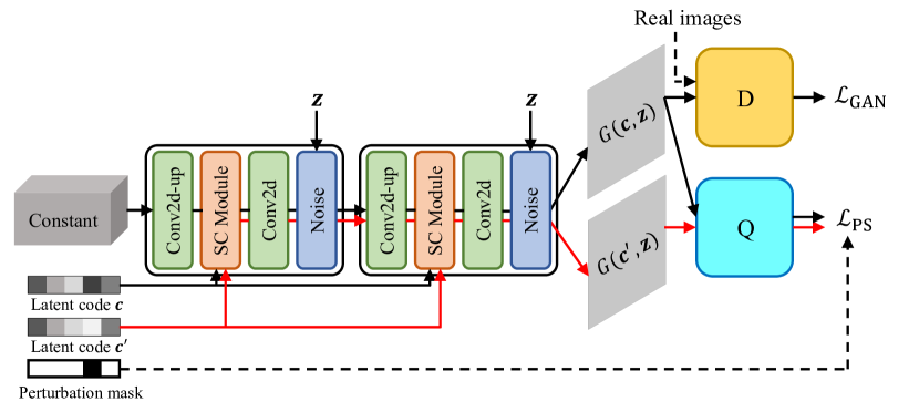
Figure 1: Overview of our proposed PS-SC model.

How can we simulate constricted modification with neural networks? For the modification procedure alone, we can adopt the idea of adaptive normalization (AdaIN), a module developed based on instance normalization for style transferring tasks [53, 15, 20, 28], and has been used for general image generation [25, 27]. The AdaIN is defined as: $\text{AdaIN}(\boldsymbol{x},\boldsymbol{y})=\sigma(\boldsymbol{y})\Big{(}\frac{\boldsymbol{x}-\mu(\boldsymbol{x})}{\sigma(\boldsymbol{x})}\Big{)}+\mu(\boldsymbol{y})$, where $\boldsymbol{x}$ denotes the content input and $\boldsymbol{y}$ denotes the style input, and $\mu$, $\sigma$ compute the mean and standard deviation across spatial dimensions. To simulate constricted modification, it is natural to consider using the heatmaps computed by the $\mathtt{softmax}$ layer in attention modules [55, 6, 36] to highlight the focused areas of a latent dimension. However the $\mathtt{softmax}$ transformation forces the activations to have a summation of 1, which is more effective for weighted aggregation of features instead of localized modification (see Sec. 4.3 for an empirical comparison). Instead, we leverage a gating layer called $\mathtt{cumax}$, an activation function proposed by [48], originally used for structured language modeling, to realize our goal. The $\mathtt{cumax}$ is defined as: $\boldsymbol{g}=\mathtt{cumax}(...)=\mathtt{cumsum}(\mathtt{softmax}(...))$, where the $\mathtt{cumsum}$ function denotes the cumulative summation. The $\mathtt{cumax}$ layer in practice transforms a vector of neurons into a soft version of binary gates $\hat{\boldsymbol{g}}=(0,...,0,1,...,1)$, since the $\mathtt{softmax}$ usually results in a hump in a vector. By combining two of this function with an element-wise product $\boldsymbol{g}=\mathtt{cumax}(...)\odot(\boldsymbol{1}-\mathtt{cumax}(...))$, we create a learnable binary gate (band-pass-filter shaped) with degrees of freedom on both ends.

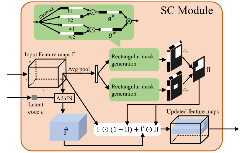
Figure 2: Detailed illustration of the SC module.

The proposed Spatial Constriction (SC) module is illustrated in Fig. 2. We use $\boldsymbol{\Gamma}$ to denote the input feature maps, and $c$ to be the input latent code. The learnable gate for the height dimension is computed as:

$$\boldsymbol{v}^{h1} =f^{h1}(\mathtt{avgpool}(\boldsymbol{\Gamma})),$$ (1)

$$\boldsymbol{v}^{h2} =f^{h2}(\mathtt{avgpool}(\boldsymbol{\Gamma})),$$ (2)

$$\boldsymbol{g}^{h} =\mathtt{cumax}(\boldsymbol{v}^{h1})\odot(\boldsymbol{1}-\mathtt{cumax}(\boldsymbol{v}^{h2}),$$ (3)

where $f^{h1}$ and $f^{h2}$ are functions to map vectors to the length of the height of the input feature maps. Similarly, we can get the gate for width dimension $\boldsymbol{g}^{w}$. A mask on feature maps is computed by performing an outer product:

$$\boldsymbol{\pi}=\boldsymbol{g}^{h}\otimes\boldsymbol{g}^{w}.$$ (4)

This is a differentiable rectangular mask with learnable sides and position. We allow a SC mask to be more flexible than a single rectangular and we use the sum of $J$ rectangles as a direct solution:

$$\boldsymbol{\Pi}=\frac{1}{J}\sum_{j=1}^{J}\boldsymbol{\pi}_{j}.$$ (5)

Then a latent code modifies the content on the input feature maps conditioned on the SC mask:

$$\hat{\boldsymbol{\Gamma}} =\text{AdaIN}(\boldsymbol{\Gamma},f(c)),$$ (6)

$$\text{SC}(\boldsymbol{\Gamma},c) =\boldsymbol{\Gamma}\odot(\boldsymbol{1}-\boldsymbol{\Pi})+\hat{\boldsymbol{\Gamma}}\odot\boldsymbol{\Pi},$$ (7)

where $\hat{\boldsymbol{\Gamma}}$ is the content modified by code $c$. Function $f$ maps code $c$ to the length of the input channel number of $\boldsymbol{\Gamma}$, which is required by AdaIN.

3.2 Encouraging Perceptual Simplicity

The second hypothesis about interpretability in representations is that the data variations captured by individual latent dimensions should be perceptually simple (see Sec. 3.3 for a quantitative example). In this section, we introduce a loss to integrate this goal into training an encoder for a GAN. We first introduce how this loss is defined, and then discuss why such a simple implementation works.

We assume a generator $G$ takes a vector of latent code $\boldsymbol{c}\in\mathbb{R}^{d}$ and a vector of noise $\boldsymbol{z}$ to generate an image: $\boldsymbol{x}=G(\boldsymbol{c},\boldsymbol{z})$, following the notations in InfoGAN [8] (see Sec 6 in the Appendix for a brief introduction about GAN and InfoGAN). The noise code $\boldsymbol{z}$ is to provide $G$ with sharp details about an image, which will be omitted in the following text, and the latent code $\boldsymbol{c}$ is to learn interpretable information. We impose a perturbation on a randomly selected dimension in the latent code $c^{\prime}_{k}=c_{k}+p$, where $k\sim\mathcal{U}_{\text{int}}(0,d-1)$, $p\sim\mathcal{N}(c_{k},p_{\text{var}})$ and $p_{\text{var}}$ is a hyper-parameter. Then we get another image $\boldsymbol{x}^{\prime}$ generated by the altered latent code $\boldsymbol{x}^{\prime}=G(\boldsymbol{c}^{\prime})$ where $\boldsymbol{c}^{\prime}=\{\boldsymbol{c}_{\setminus k},c^{\prime}_{k}\}$ . Then we introduce a recognizer $Q$, whose primary goal is to reconstruct the latent code $\boldsymbol{c}$ and $\boldsymbol{c}^{\prime}$ based on the generated images $\boldsymbol{x}$ and $\boldsymbol{x}^{\prime}$ ($\hat{\boldsymbol{c}}=Q(\boldsymbol{x})$, $\hat{\boldsymbol{c}}^{\prime}=Q(\boldsymbol{x}^{\prime})$) respectively with MSE loss. However, in order to enforce the simple encoding along dimensions of the latent code, we substitute the errors computed on the shared dimensions by the errors between the truth code and the average of both reconstructed values, leading to the dimension-wise loss defined as:

$$loss_{i}=\begin{cases}(\hat{c}_{i}-c_{i})^{2}+(\hat{c}^{\prime}_{i}-c^{\prime}_{i})^{2},&\text{if }i=k\\ 2\times(\frac{\hat{c}_{i}+\hat{c}^{\prime}_{i}}{2}-c_{i})^{2},&\text{if }i\neq k\end{cases},$$ (8)

where the $\hat{\boldsymbol{c}}$ and $\hat{\boldsymbol{c}}^{\prime}$ are outputs from $Q$, and $k$ is the perturbed dimension index. Note that $c_{i}=c^{\prime}_{i}$ if $i\neq k$. We sum the losses on all dimensions to form the complete loss, which is named as Perceptual Simplicity (PS) loss:

$$\mathcal{L}_{\text{PS}} =\frac{1}{d}\sum_{i=0}^{d-1}loss_{i}.$$ (9)

This is similar to an ordinary reconstruction loss on latent codes, but with the losses on shared dimensions calculated in a fuzzy way.

Discussion: The PS loss is more tolerant of the misalignment on the shared dimensions than on the perturbed dimension, since it only requires the mean of the shared two latent-code reconstructions to match the truth code. In other words, the loss will punish the model more on the mistakes made along the non-shared dimension than on the other directions, forcing the generator to embed more easily recognizable variations along this specific latent axis so that the recognizer $Q$ can more easily regress to the truth value on this dimension. Since the non-shared dimension is randomly selected in each iteration, after convergence the $Q$ will still be an encoder. The generator $G$ should find a solution that the data variations controlled by each latent dimension are necessarily simple to be interpreted, but the coupled data variations controlled by all dimensions are rich enough to form data matching the training distribution. Our PS loss is similar to a series of losses from VAE-based models [3, 19, 42], but the paired images used in these works are picked by varying a known attribute with supervision, while ours does not rely on any labels.

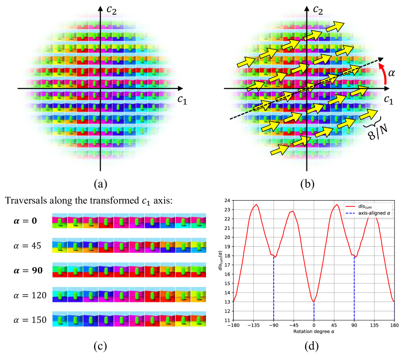
Figure 3: (a) A 2D disentangled representation capturing semantics of pure wall color and floor color. (b) Illustration of how the $\text{dis}_{cum}$ (Eq. 10) is quantified in the $(c_{1},c_{2})$ space. Perceptual distance scores along yellow arrows are accumulated. (c) Latent traversals for different $\alpha$’s along axis $c_{1}$. (d) The plot showing how the $\text{dis}_{cum}$ value changes with rotation degree $\alpha$.

3.3 Traversal Perceptual Length

In this section, we first show a concrete example of the Perceptual Simplicity assumption in interpretability, then we introduce an unsupervised model selection method.

Fig. 3 (a) shows a disentangled representation (with $c_{1}$ and $c_{2}$ dimensions) capturing two data variations from 3DShapes dataset [29] (wall color vs floor color). This representation is interpretable since we can tell that each dimension encodes pure wall color and floor color respectively. Then we apply a rotation on the coordinate system in this latent space by $\alpha$ degrees as shown in Fig. 3 (b). Because standard Gaussian distribution is rotation-invariant, this transformation does not break the statistical independence property of the representation. However it breaks the interpretability property since the traversals along individual axes are not controlling pure variations (see traversals in Fig. 3 (c)). This absence of interpretability is noticeable by humans, but can a model sense it without labels? To show this is possible, we define the accumulated perceptual distance ($\text{dis}_{cum}$) by traversing along the transformed $c_{1}$ axis in the 2D space (see Fig. 3 (b) for an illustration):

$$\text{dis}_{cum}(\alpha)=\sum_{\mathclap{\begin{subarray}{c}(c_{1},c_{2})\in\text{grid}(-4,4)\end{subarray}}}\text{dis}\Big{(} G\big{(}\mathtt{R}(\alpha)(c_{1},c_{2})\big{)},$$

$$G\big{(}\mathtt{R}(\alpha)(c_{1}+\frac{8}{N},c_{2})\big{)}\Big{)},$$ (10)

where $\text{grid}(-4,4)$ is an $N\times N$ grid with coordinates ranging from $-4$ to $4$, and $\text{dis}(...)$ denotes perceptual distance computation using VGG16 [49]. The $\mathtt{R}(\alpha)$ is a rotation matrix in 2D space parameterized by degree $\alpha$. The plot of $\text{dis}_{cum}$ vs $\alpha$ is in Fig. 3 (d). As we can see, when the coordinate system is aligned with the interpretable axes in Fig. 3 (a) ($\alpha=-90,0,90,180$), the $\text{dis}_{cum}$ scores become local minima (indicated by the blue dash lines). This experiment indicates that though a disentangled representation is indeed isotropic in terms of statistical independence, it is perceptually anisotropic, with variations along latent axes being simpler than other directions (more examples are shown in the Appendix Sec. 8).

This perceptual-anisotropy phenomenon inspires us to develop an unsupervised model selection method, since we can assume the overall accumulated perceptual distance scores along all latent axes to be generally small in disentangled representations. The method, namely Traversal Perceptual Length (TPL), is defined as follows:

tpl $${}_{i}(G)=\mathbb{E}_{\boldsymbol{c}}\sum_{\mathclap{c_{i}\in\text{lin}(-4,4)}}\text{dis}\big{(}G(\boldsymbol{c}_{\backslash i},c_{i}),G(\boldsymbol{c}_{\backslash i},c_{i}+\frac{8}{N})\big{)},$$ (11)

tpl $$(G)=\sum_{i=0}^{d-1}\text{act}_{i}\cdot\text{tpl}_{i}(G),\quad\text{act}_{i}=\begin{cases}1,&\text{tpl}_{i}(G)\geq S\\ 0,&\text{tpl}_{i}(G)<S\\ \end{cases},$$ (12)

where $\text{lin}(-4,4)$ denotes linearly spaced $N$ values in interval $(-4,4)$, and $S$ is a threshold to determine if a dimension encodes enough information to be activated. Our method is different from existing model selection methods [12] and unsupervised metrics [25, 60] in ways like: 1) it does not rely on comparing a herd of models; 2) it does not rely on training a classifier; 3) it approximately evaluates interpretability along axes. More Pros and Cons are shown in the Appendix Sec. 9.

4 Experiments

In this section we evaluate the proposed TPL model selection method, and the effectiveness of our interpretability-oriented models for learning disentangled representations. The introductions of the used datasets and implementations are in the Appendix Sec. 7 and Sec. 14 respectively. Code is available at https://github.com/zhuxinqimac/PS-SC.

4.1 Effectiveness of TPL

We first conduct experiments to evaluate the effectiveness of the proposed TPL model selection method. An intuitive way to do so is by examining its agreement with existing supervised metrics applied on existing disentanglement learning models. Specifically, we compute the TPL scores (the threshold $S$ is set to be 0.01 and the number of segments $N$ is set to be 50) on 1,800 pretrained checkpoints from [41] on DSprites dataset and then compute the correlation coefficients against four supervised metrics: $\beta$-VAE metric (BVM) [18], FactorVAE metric (FVM) [29], DCI disentanglement score [14], and Mutual Information Gap (MIG) [7]. The pretrained checkpoints include 6 different models ($\beta$-VAE [18], FactorVAE [29], DIP-VAE I and II [33], $\beta$-TC-VAE [7], and Annealed VAE [4]), covering 6 hyper-parameter configurations each and 50 random seeds each. These configurations form an extensive coverage from good models to bad models.

Range	Methods	BVM	DCI	FVM	MIG
All	TPL (act$>$0)	0.15	0.44	0.21	0.49
	TPL (act$>$4)	0.45	0.72	0.60	0.66
	FVM	0.82	0.77	1.00	0.72
TC-VAE	UDR	0.42	0.55	0.30	0.37
	TPL (act$>$0)	0.39	0.79	0.39	0.73

Table 1: Spearman’s rank correlation between unsupervised model selection methods and supervised disentanglement metrics.

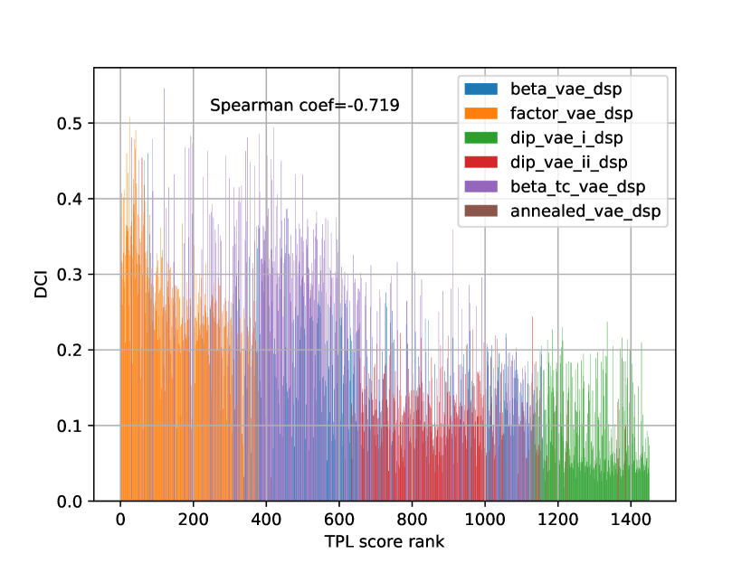
Figure 4: TPL (act$>$4) vs DCI disentanglement on DSprites dataset across various configurations. Ranked by TPL scores.

In Table 1 upper part we show the Spearman’s rank correlation scores computed over all models thresholded by the number of active latent dimensions (the active dimensions are determined by TPL without supervision). The reason we threshold the models by active latent dimensions is that the TPL can be misled by cheating models which achieve disentanglement by only encoding a subset of generative factors. These models are indeed disentangled if they are evaluated based only on this subset of factors, but will not be ranked high if compared against all the ground-truth factors as done by supervised metrics. However, our TPL is an unsupervised method and has no access to the ground-truth factors, thus may wrongly rank those cheating models high, leading to lower correlation with supervised metrics as shown by the entry act$>$0 in Table 1 (there are 5 ground-truth factors). Fortunately these models can be directly filtered out by the number of active dimensions computed by TPL, and in real-world applications they can also be filtered out by unsupervised generative quality metrics like FID [17], ensuring TPL to work in its more effective zone. The TPL (act$>$4) works reasonably well for ranking the pretrained models. The supervised FVM row works as an upper bound, and the largest difference between TPL and FVM is the correlation with BVM, indicating the TPL is more similar to DCI and MIG metrics while different from BVM. In the lower part of Table 1 we compare our model against UDR unsupervised metric on the model TC-VAE (UDR scores calculated on all models are not available). Our method correlates better with supervised metrics, especially DCI and MIG. The plot of TPL (act$>$4) vs DCI metric is shown in Fig. 4, where the models are ranked by TPL. An obvious descending trend can be observed, indicating the TPL roughly sorts the models in a correct way. As we plot different models with different colors, we see that among the 6 models, FactorVAE and TC-VAE are most promising for disentanglement learning, which agrees with our common sense in this field. More correlation results and more plots for other metrics and other numbers of active dimensions are shown in the Appendix Sec. 10. This experiment also implies that our hypothesis of Perceptual Simplicity holds in general disentangled representations learned by existing models.

4.2 Shoes and Clevr

Methods	Shoes+Edges		Clevr-Simple		Clevr-Comp
	PPL	FID	PPL	FID	PPL	FID
InfoGAN	2952.2	10.4	56.2	2.9	83.9	4.2
HP	1301.3	21.2	45.7	25.0	73.1	21.1
HP+FT	554.1	17.3	39.7	6.1	74.7	7.1
Ours	246.2	9.7	9.2	9.2	17.4	10.8

Table 2: Comparing Perceptual Path Length (PPL) and Fréchet Inception Distance (FID) on Edge+Shoes and Clevr datasets. Lower is better for both metrics.

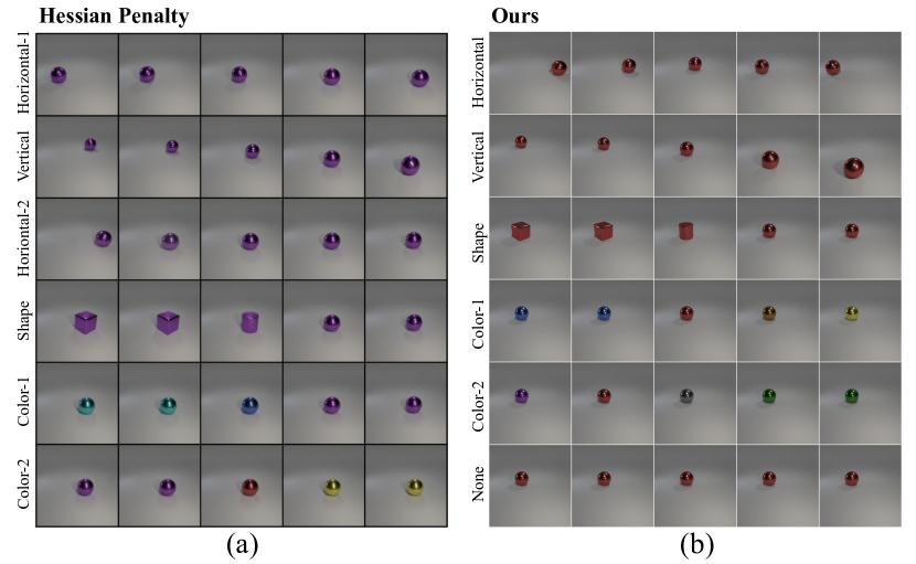
Figure 5: Qualitative comparison between Hessian Penalty model [45] and ours on Clevr-Simple dataset.

We follow the setups in [45] to conduct experiments on the Shoes+Edges dataset (created by mixing 50,000 edges and 50,000 shoes) [58], and variants of Clevr dataset [23]: Clevr-Simple contains four factors of variation: object color, shape, and location (10,000 images); Clevr-Complex contains two objects of Clevr-Simple in multiple sizes (10,000 images). Table 2 shows the quantitative comparison between our model and multiple baselines provided by [45], using the same metrics Perceptual Path Length (PPL) [25] and Fréchet Inception Distance (FID) [17]. It is clear our model outperforms the baselines significantly. Note that HP+FT is a fine-tuned model based on a pretrained ProGAN [24], thus the direct end-to-end trained baseline should be the HP version. Our models work best in terms of disentanglement on all datasets, and on Shoes+Edges ours can even achieve the best FID score. On Clevr datasets, our models have worse FID, which may be caused by the smaller size of the datasets, which consist of more factors of variations than Shoes+Edges but have fewer data samples to train.

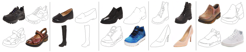
Figure 6: Shoes $\leftrightarrow$ Edges translation by altering the dimension corresponding to the domain concept.

In Fig. 5 we qualitatively compare the representations learned by a HP baseline and our model on Clevr-Simple dataset. We show the latent traversals of the learned latent codes (baseline images are taken from [45]), ordered from high to low by our defined $\text{tpl}_{i}$ in Eq. 11. We can see our model encodes the vertical and horizontal position variations into two clear separate latent codes, while the baseline encodes these two factors into three codes. In Fig. 6 we show that our model encode the domain concept in a single latent dimension on the Shoes+Edges dataset. We achieve such a domain shift by just reversing the sign of this single dimension in the representation.

4.3 CelebA and FFHQ

We conduct experiments on human-face datasets CelebA [39] and FFHQ [25]. For CelebA we crop the center $128\times 128$ area, and for FFHQ we use the $512\times 512$ version.

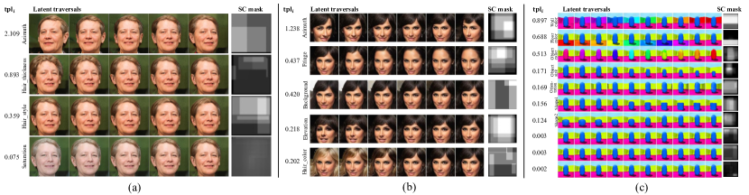
Figure 7: (a) Latent traversals on FFHQ dataset ordered by $\text{tpl}_{i}$ scores. The masks coarsely highlight the corresponded components in images. (b) Same results on CelebA dataset. (c) Same results on 3DShapes dataset.

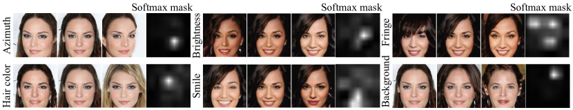
Figure 8: Latent traversals by models trained with softmax masks.

Methods	CelebA			FFHQ
	TPL	PPL	FID	TPL	PPL	FID
InfoGAN	10.9	43.6	6.0	33.4	142.7	11.0
+PS Loss	8.5	34.3	6.2	30.7	139.6	13.8
+SC Module	9.9	44.1	5.9	20.4	136.5	16.4
+Both	8.1	38.9	6.0	18.7	120.1	13.5

Table 3: Ablation study about different modules on CelebA and FFHQ datasets.

Methods	CelebA			FFHQ
	TPL	PPL	FID	TPL	PPL	FID
softmax-mask	14.8	49.3	18.4	28.3	145.4	57.1
$\lambda=$ 0.001	10.2	47.5	5.3	20.3	135.4	23.7
$\lambda=$ 0.01	8.1	38.9	6.0	18.7	120.1	13.5
$\lambda=$ 0.1	9.1	42.0	7.2	20.0	123.2	16.0

Table 4: Ablation study about softmax mask and $\lambda$ on CelebA and FFHQ datasets.

For quantitative evaluation, the FID metric is used to evaluate generative quality, and the PPL and TPL (the threshold $S$ is set to be 0.3 on CelebA and 0.5 on FFHQ, the number of segments $N$ is set to be 48) are used for rough measurement of disentanglement. On CelebA we train models for around 19 epochs, and on FFHQ we train models for around 28 epochs where FID starts to saturate. In Table 3 we evaluate the effectiveness of the proposed Perceptual Simplicity loss and the Spatial Constriction module. Both modules improve the baseline model in terms of disentanglement, validated by both the PPL metric and our TPL scores. Note that the PPL measures the perceptual smoothness of the latent space but cannot detect if a latent axis captures simple variations, while TPL can perform a rough evaluation on this property of interpretability. This is why the PPL and TPL disagree on the +PS and +Both rows, where the additional SC module slightly sacrifices the overall smoothness in the latent space to achieve an alignment between simple variations and latent axes. On both datasets, the two contributions can be combined to achieve the best performance, indicating their complimentarity. Then we evaluate how the strength of PS loss impact the learning of models. We denote the trade-off between the GAN loss and PS loss by a hyper-parameter $\lambda$ : $\mathcal{L}_{total}=\mathcal{L}_{GAN}+\lambda\mathcal{L}_{PS}$. Table 4 shows the ablation study. We see setting $\lambda=0.01$ is generally a good choice for both datasets, while when it increases to 0.1 both models appear to degenerate in generation ability. For CelebA, setting $\lambda=0.001$ is beneficial to the image synthesis, but on FFHQ this harms the image quality. It indicates this $\lambda$ is too small for the model to maintain good generation ability on this high-resolution dataset with less training samples, probably due to that the effect of the latent reconstruction loss as a regularization has been wiped out. The experiment of switching the SC masks to softmax masks is also shown in the Table 4. We see using softmax masks is not an ideal choice since it harms both the disentanglement and the generation quality. This is also qualitatively verified by comparing the latent traversals shown in Fig. 8 and Fig. 7 (b). The ablation study on the number of rectangles $J$ used in SC modules is shown in the Appendix Sec. 11.

For qualitative evaluation, we show the latent traversals and the learned SC masks on both datasets in Fig. 7 (a) (b). More traversals are shown in the Appendix Sec. 12 and traversals.gif in the supplementary. We observe that 1) many semantics in these two datasets are successfully captured by individual latent dimensions, including some subtle variations like the hair thickness, hair style on FFHQ, and the elevation on CelebA; 2) the dim-wise TPL score ($\text{tpl}_{i}$) agrees with human’s common sense about the significance of the discovered semantics, indicating it can be used to filter out non-significant noise information, or automatically detect important variations; 3) the SC masks coarsely align with the components controlled by each latent code, masks for azimuth and elevation covering main areas in the images, masks for hair related information covering upper part of the images, . Compared to the masks learned by softmax shown in Fig. 8, the SC masks are more informative and interpretable, and the softmax masks usually consist of point-like heatmaps. Though the softmax masks are sometimes meaningful like the ones corresponding to smile and fringe, masks for most other semantics are not interpretable, resulting in worse disentanglement quality than using SC masks. Notice that in Fig. 7 (a) the dimension capturing saturation is assigned with a very low $\text{tpl}_{i}$ score. This is due to the bias of perceptual distance used in the score computation, which is more sensitive to high-level semantic variations. In Fig. 9, we compare the latent traversals between our model and two existing GAN-based models on CelebA ($128\times 128$ version). Though all three models seem to discover the shown semantics, the InfoGAN-CR has the worst disentanglement quality (e.g. lighting entangled with smile). Moreover, both baselines cannot maintain a high generative quality when constrained to disentangle the underlying semantic factors. Unlike either of them, our model can achieve high-quality disentanglement while maintaining much better generative quality.

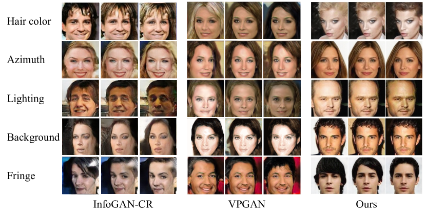
Figure 9: Latent traversal comparison on CelebA dataset between InfoGAN-CR [38], VPGAN [60], and our model.

Model		DSprites	3DShapes
VAE	VAE	63 (6)	-
	$\beta$-VAE	74.41 (7.68)	91 (from [29])
	CascadeVAE	81.74 (2.97)	-
	FactorVAE	82.15 (0.88)	89 (from [29])
GAN	InfoGAN	65.41 (7.03)	83.65 (9.49)
	IB-GAN	80 (7)	-
	InfoGAN-CR	88 (1)	-
	Ours	83.54 (6.91)	92.04 (6.49)
	Ours+TPL	84.22 (4.21)	93.41 (3.34)

Table 5: State-of-the-art comparison using FactorVAE metric on DSprites and 3DShapes datasets.

We then conduct an image editing experiment with our trained model on FFHQ. Specifically, we generated a set of source images to provide main attributes, and another set of images to provide the new attributes. Afterwards we copy the latent code dimensions representing new attributes to the corresponding positions in the latent code of the source images. The results are shown in Fig. 10. We see the source images are naturally adapted to the given attributes, while keeping the other attributes intact. More image editing examples are in the Appendix Sec. 13.

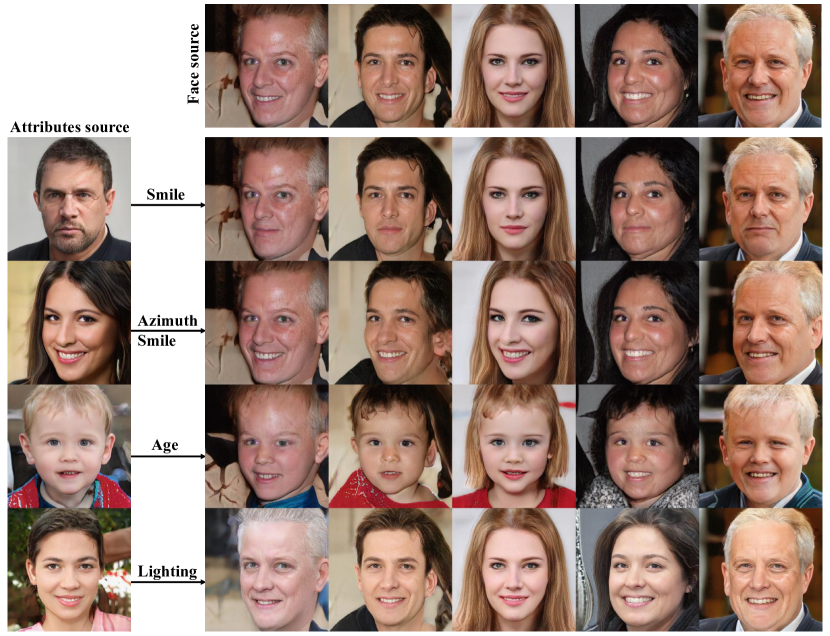
Figure 10: Top row: source images. Left column: images providing attributes. Main section: transformed images using the provided attributes from the left ones.

4.4 DSprites and 3DShapes

In Table 5 we compare the state-of-the-art models trained with continuous latent codes on DSprites and 3DShapes synthetic datasets. 10 random seeds are used to train the models, and for the +TPL version we use 30 seeds to train and report results with the top 10 seeds ranked by our unsupervised TPL model selection method. On DSprites the InfoGAN-CR achieves the best performance, but it was trained by keeping the number of latent dimensions equal to the ground-truth factors, which is different from the general over-parameterized setting. Our model shown on DSprites does not use SC module since the Spatial Constriction assumption does not hold on this synthetic dataset and using SC module harms the performance (obtaining a score of 81.47 (5.39)). On 3DShapes our model achieves the best performance, and a latent traversal is shown in Fig. 7 (c).

5 Conclusion

Based on the observation that interpretability usually comes from localized and simple variations, we proposed to learn disentangled representations by directly modeling interpretability from these two perspectives as a proxy. We adopted two hypotheses, Spatial Constriction and Perceptual Simplicity, to construct our models. We designed a module to constrain the impact of each latent dimension into constricted subareas, and a loss to enforce the encoding of simple variations along latent axes. We also introduced a simple unsupervised model selection method by quantifying the perceptual variations accumulated along latent axes. Experiments on various datasets validated the effectiveness of our proposed modules and the model selection method. Although our work was proposed as a standalone approach for learning disentangled representations, it should work together with other assumptions like statistical independence to achieve a boosted performance, and we left this exploration for future work.

Appendix

6 GAN and InfoGAN

The Generative Adversarial Network [16] is a generative model trained via a minimax game performed between a generator $G$ and a discriminator $D$:

$$\underset{G}{\text{min}}\,\underset{D}{\text{max}}\,V(G,D) =\mathbb{E}_{\boldsymbol{x}\sim p_{\text{data}}}[\text{log}\,D(\boldsymbol{x})]$$

$$+\mathbb{E}_{\boldsymbol{z}\sim p_{\text{noise}}}[\text{log}\,(1-D(G(\boldsymbol{z})))],$$ (13)

where $\boldsymbol{z}$ is a noise variable sampled from a prior distribution $p_{\text{noise}}(\boldsymbol{z})$, the generator $G$ maps $\boldsymbol{z}$ to the pixel space to synthesize images, and the discriminator $D$ predictes if an images is sampled from the real distribution or not. After convergence, the $G$ should be able to synthesize realistic images and the $D$ cannot tell if an image is fake or not.

The InfoGAN [8] augments the GAN loss (Eq. 13) with a regularization term:

$$\underset{G,Q}{\text{min}}\,\underset{D}{\text{max}}\,V_{\text{INFO}}(G,D)=V(G,D)-\beta I(\boldsymbol{c};G(\boldsymbol{c},\boldsymbol{z})),$$ (14)

where $I(\boldsymbol{c};G(\boldsymbol{c},\boldsymbol{z}))$ is the mutual information between a subset of latent codes $\boldsymbol{c}\in\mathbb{R}^{d}$ and the generated samples $G(\boldsymbol{c},\boldsymbol{z})$. By maximizing the mutual information, the latent codes $\boldsymbol{c}$ are able to represent a set of interpretable salient variations in data. In practice, the mutual information is approximated by a variational lower bound and is implemented with an auxiliary network $Q$, trained together with $G$ by regression loss for predicting the latent codes $\boldsymbol{c}$.

7 Datasets Introduction

CelebA

This is a dataset of 202,599 images of cropped real-world human faces, containing various poses, backgrounds and facial expressions. We use the cropped center $128\times 128$ area in this paper.

Shoes+Edges

This dataset contains the commonly used image-to-image translation datasets Shoes and Edges, but mixes the 50,000 Shoes images and 50,000 Edges images together to form a 100,000-image dataset in 128$\times$128.

Clevr-Simple

This dataset is a variant of the Clevr dataset, which contains an object featuring four factors of variation: object color, shape, and location (both horizontal and vertical). It contains 10,000 256$\times$256 images.

Clevr-Complex

This dataset retains all variations from Clevr-Simple but adds a second object and multiple sizes for a total of 10 factors of variation (5 per object). It contains 10,000 256$\times$256 images.

FFHQ

This is a dataset of aligned images of human faces crawled from Flickr (70,000 in tatal). We use the $512\times 512$ version in our paper. Link: https://github.com/NVlabs/ffhq-dataset.

DSprites

This is a dataset of 2D shapes generated from 5 independent factors, which are shape (3 values), scale (6 values), orientation (40 values), x position (32 values), and y position (32 values). All combinations are present exactly once, with the total number of binary $64\times 64$ images 737,280. Link: https://github.com/deepmind/dsprites-dataset.

3DShapes

This is a dataset of 3D shapes generated from 6 independent factors, which are floor color (10 values), wall color (10 values), object color (10 values), scale (8 values), shape (4 values), orientation (15 values). All combinations are present exactly once, with the total number of $64\times 64$ images 480,000. Link: https://github.com/deepmind/3d-shapes.

8 More Experiments of Rotating Latent Space

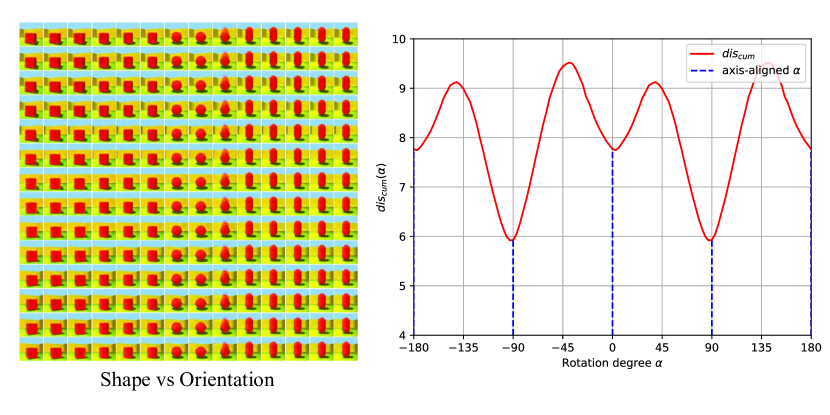
Figure 11: Shape vs Orientation.

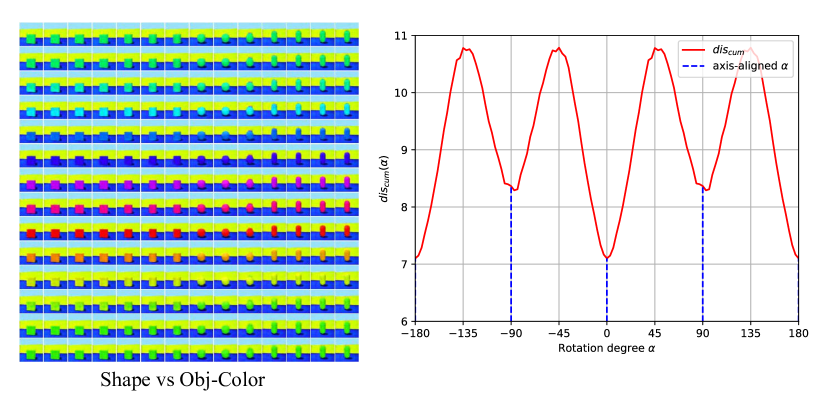
Figure 12: Shape vs Obj-Color.

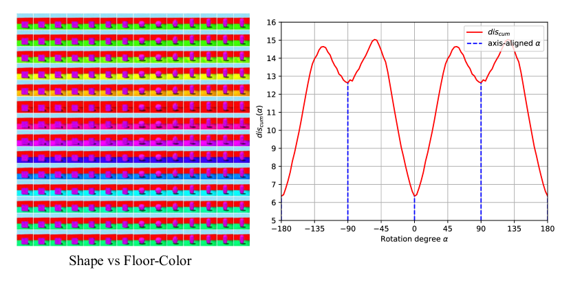
Figure 13: Shape vs Floor-Color.

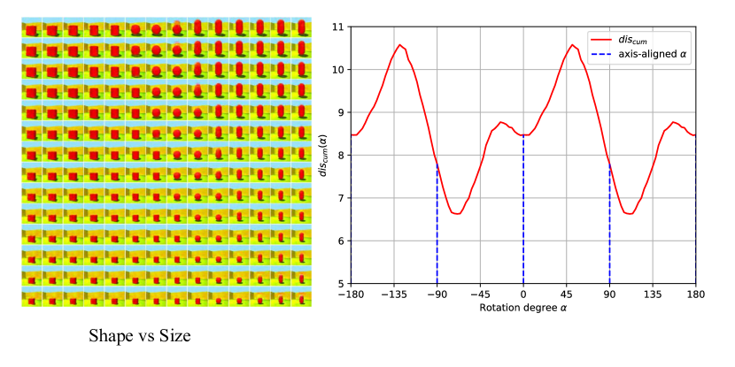
Figure 14: Shape vs Size.

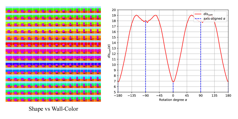
Figure 15: Shape vs Wall-Color.

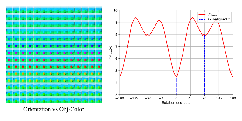
Figure 16: Orientation vs Obj-Color.

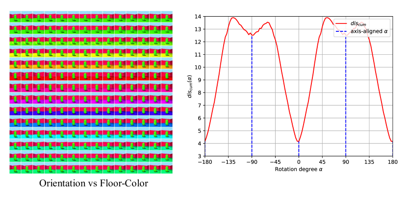
Figure 17: Orientation vs Floor-Color.

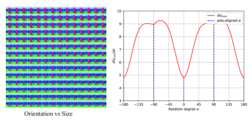
Figure 18: Orientation vs Size.

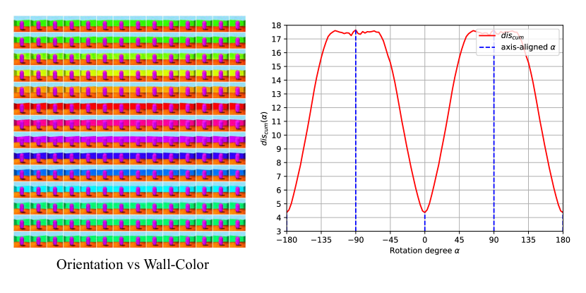
Figure 19: Orientation vs Wall-Color.

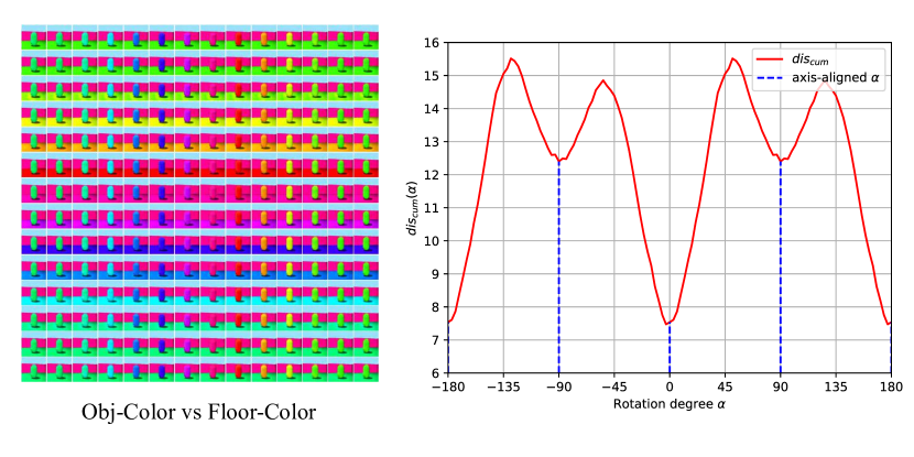
Figure 20: Obj-Color vs Floor-Color.

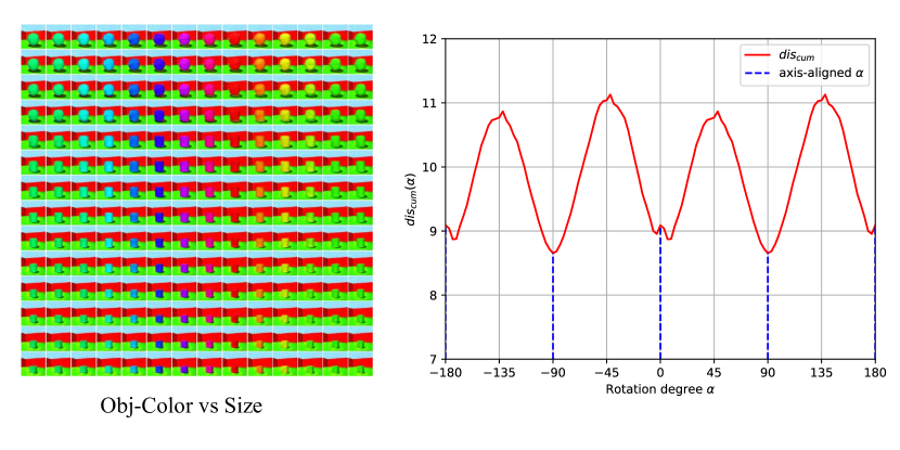
Figure 21: Obj-Color vs Size.

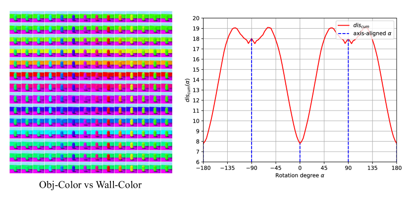
Figure 22: Obj-Color vs Wall-Color.

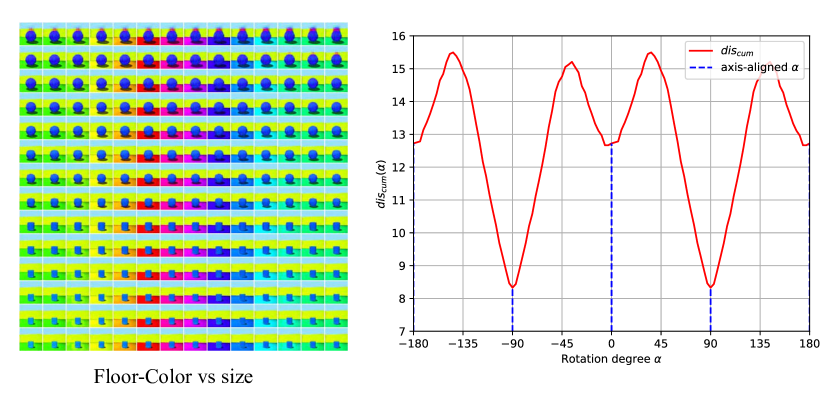
Figure 23: Floor-Color vs Size.

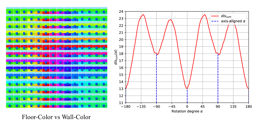
Figure 24: Floor-Color vs Wall-Color.

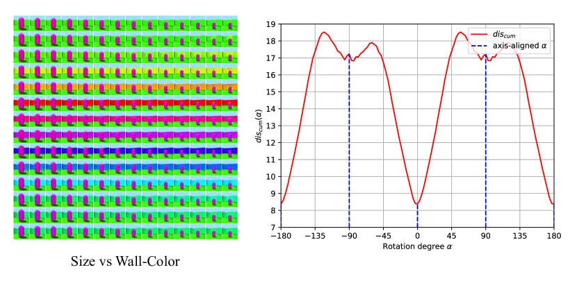
Figure 25: Size vs Wall-Color.

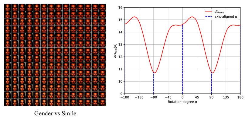
Figure 26: Gender vs Smile.

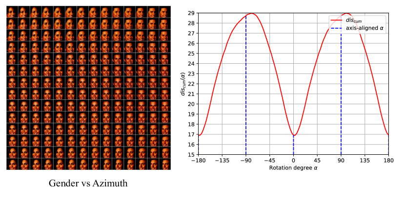
Figure 27: Gender vs Azimuth.

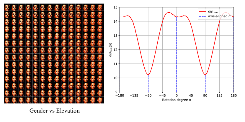
Figure 28: Gender vs Elevation.

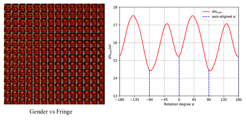
Figure 29: Gender vs Fringe.

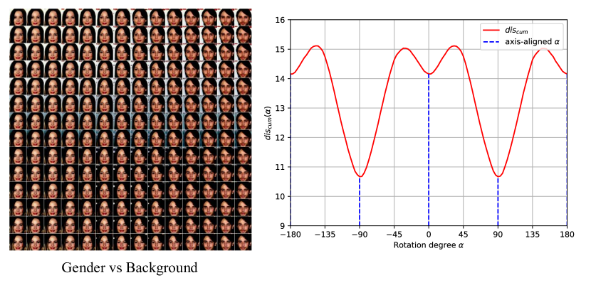
Figure 30: Gender vs Background.

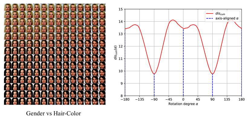
Figure 31: Gender vs Hair-Color.

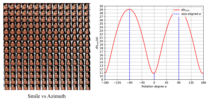
Figure 32: Smile vs Azimuth.

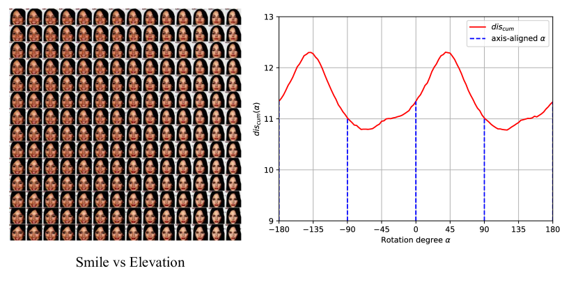
Figure 33: Smile vs Elevation.

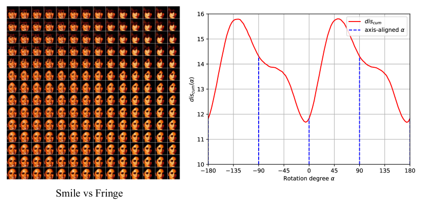
Figure 34: Smile vs Fringe.

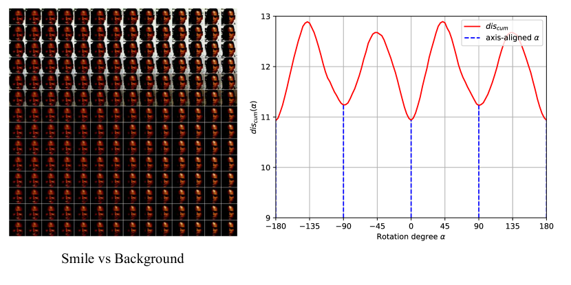
Figure 35: Smile vs Background.

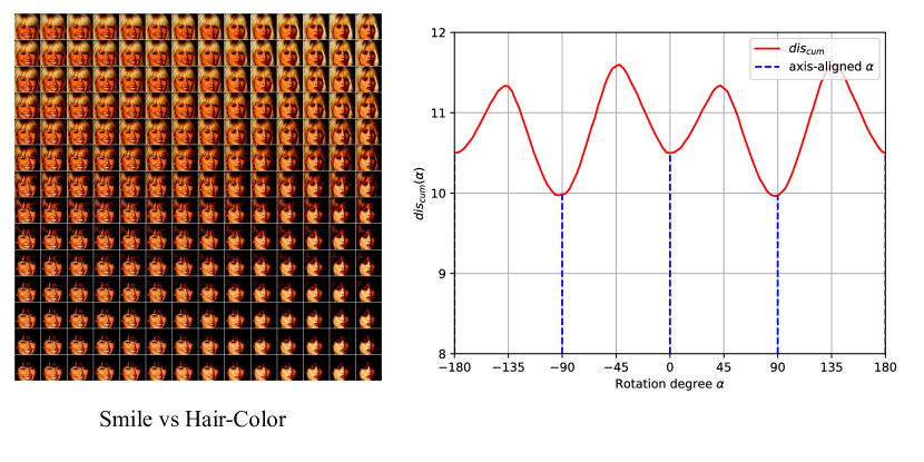
Figure 36: Smile vs Hair-Color.

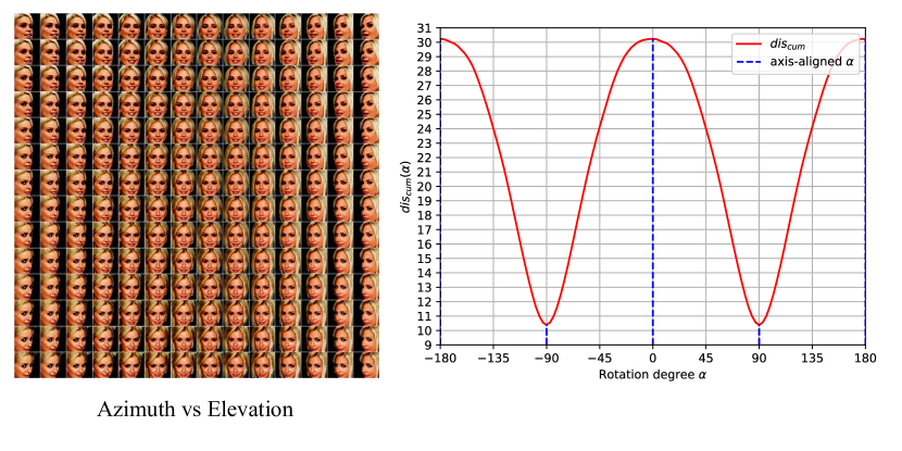
Figure 37: Azimuth vs Elevation.

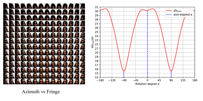
Figure 38: Azimuth vs Fringe.

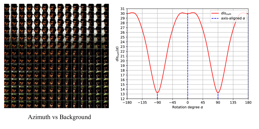
Figure 39: Azimuth vs Background.

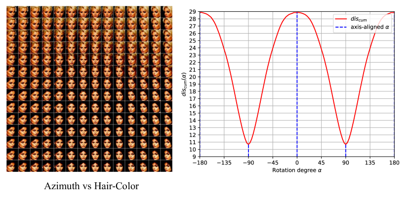
Figure 40: Azimuth vs Hair-Color.

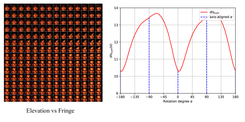
Figure 41: Elevation vs Fringe.

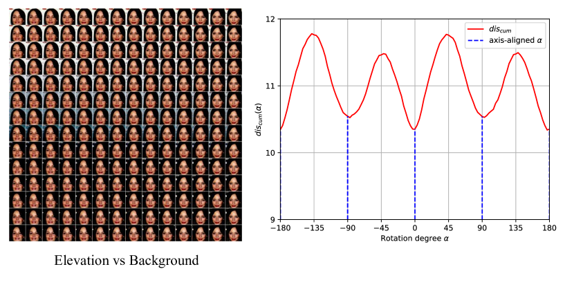
Figure 42: Elevation vs Background.

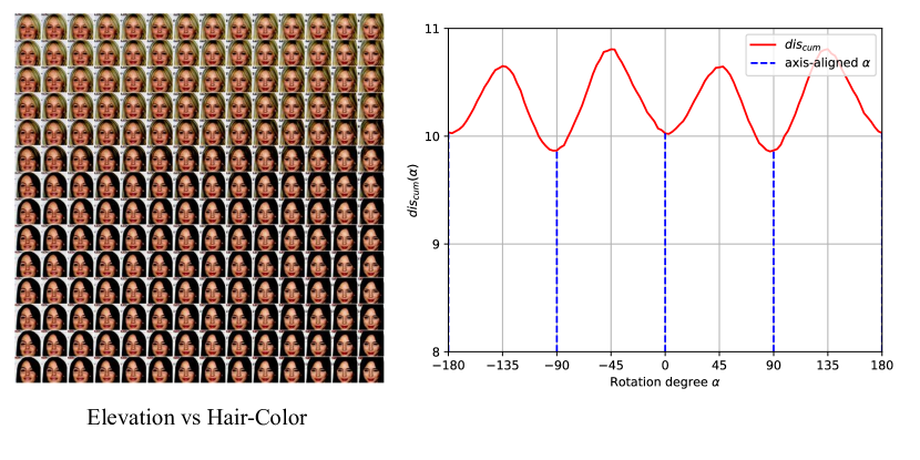
Figure 43: Elevation vs Hair-Color.

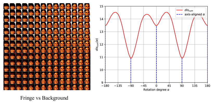
Figure 44: Fringe vs Background.

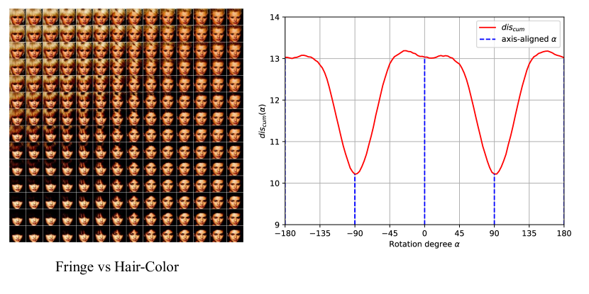
Figure 45: Fringe vs Hair-Color.

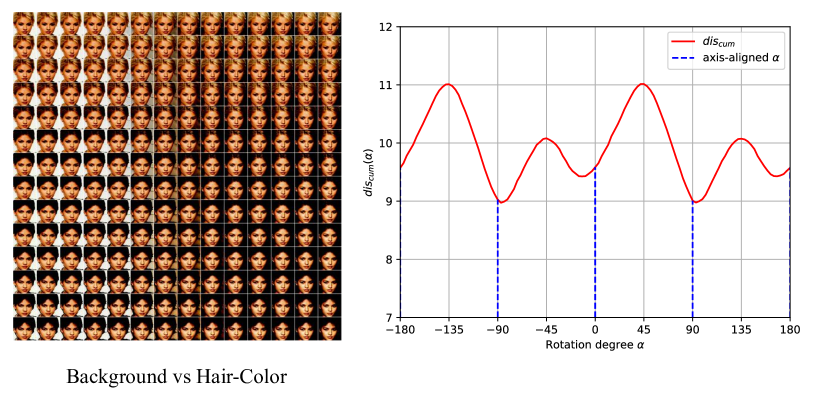
Figure 46: Background vs Hair-Color.

The plot for different semantic-pairs on 3DShapes are shown in Fig. 11 - 25. Similar results for CelebA are shown in Fig. 26 - 46. For most semantic-pairs, the corresponding $\alpha$ rotation plots agree with the assumption of Perceptual Simplicity, the accumulated perceptual distance scores become local minima when the accumulation directions are aligned with the latent axes ($\alpha=-180,-90,0,90,180$). However, there exist still some exceptions, such as Shape vs Size, and some attributes plotted against Azimuth, . These are (1) sometimes due to the imperfectly learned representations which are not fully disentangled, and (2) sometimes due to the domination of variations encoded by one dimension over another (Azimuth), leading the Perceptual Simplicity phenomenon not obvious. But in general, the assumption holds for most semantic-pairs.

9 TPL Pros and Cons

Pros: 1) Unlike [12], the TPL computation does not rely on pair-wise comparisons among a herd of models (trained with different hyper-parameters and seeds) to assign a score to a single model. This ensures the TPL is a more efficient method for model selection, and also enables its ability to work as a rough unsupervised metric to evaluate disentanglement quality. 2) Unlike [60], the TPL does not need to train an extra classifier to assign a score to a model, indicating it is a more general and efficient approach. 3) Unlike [25], the TPL leverage the perceptual anisotropy in a disentangled representation, which can select more interpretable ones than the PPL proposed in [25] which only assign a score to a model by only evaluating the perceptual smoothness in the latent space.

Cons: 1) The TPL scores can be biased by the generative ability of the generator, it usually ranks a blurred-image generator higher than a more-detailed-image generator even their disentanglement levels are similar. To alleviate this problem, we recommend using TPL together with some generative quality metrics (FID, IS) to filter out the cheating models that achieve disentanglement at the severe cost of generative quality. 2) The TPL is based on the assumption that disentangled representations contain perceptually simple variations along their latent axes. This assumption may not hold for every dataset or for every concept. In those case, supervised disentanglement learning methods may be more preferable.

10 More Results of TPL Experiments

Here we show more correlation plots for more metrics and the dimensions using the pretrained checkpoints. The correlation coefficients for each setting are shown in the plots. In Fig. 47, 48, 49, and 50, we show the plots with all dimensions of activation (act$>$0) taken into account. There are descending trends shown in each figure, but the reason that the correlation scores are low is due to the left most samples (around $<$250) shown in each plot. These samples are strangely positioned at the top of the whole rank by TPL, but are generally not scored high by supervised metrics. This is because these samples encode only a subset of factors in the dataset (3 out of 5), and some of them are detected by the supervised metrics and are assigned with low scores. In Fig. 51, 52, 53, 54, 55, 56, 57 and 58, we show the plots of samples with active dimensions larger than 3 and 4. In these figures, the TPL ranks these models much better, and the correlation coefficients also agree with the descending trends better in these plots.

Figure 47: TPL (act$>$0) vs MIG. Ranked by TPL scores.

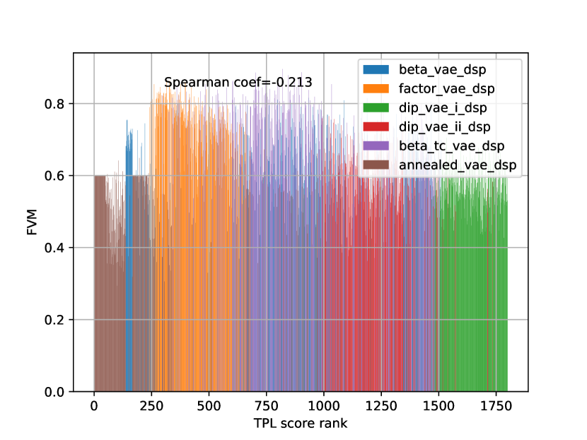
Figure 48: TPL (act$>$0) vs FVM. Ranked by TPL scores.

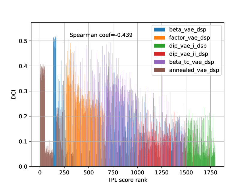
Figure 49: TPL (act$>$0) vs DCI. Ranked by TPL scores.

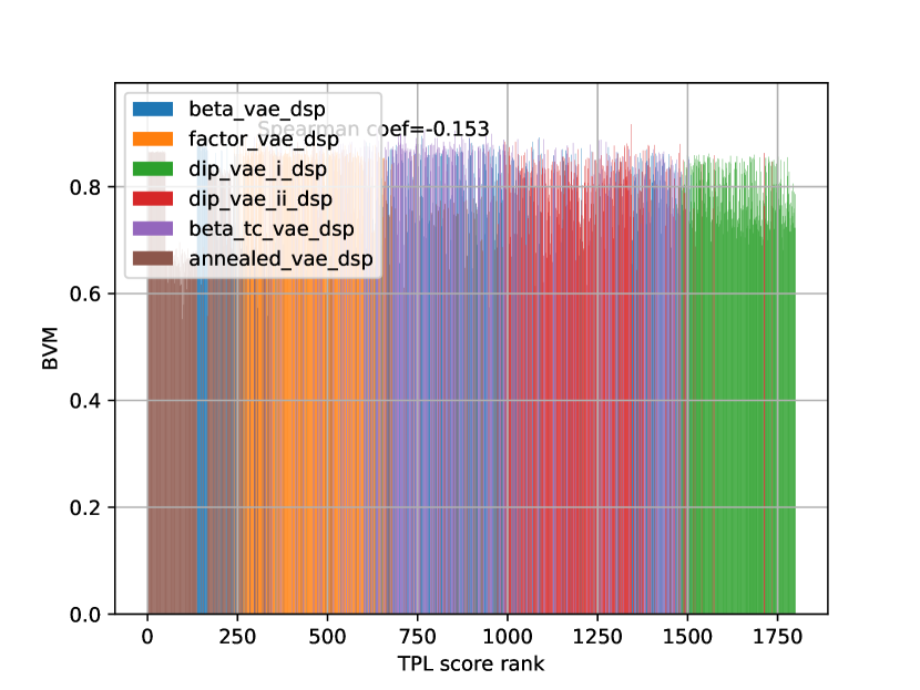
Figure 50: TPL (act$>$0) vs BVM. Ranked by TPL scores.

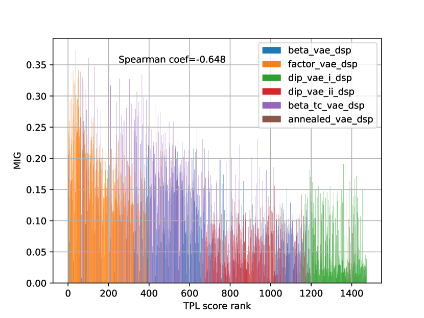
Figure 51: TPL (act$>$3) vs MIG. Ranked by TPL scores.

Figure 52: TPL (act$>$3) vs FVM. Ranked by TPL scores.

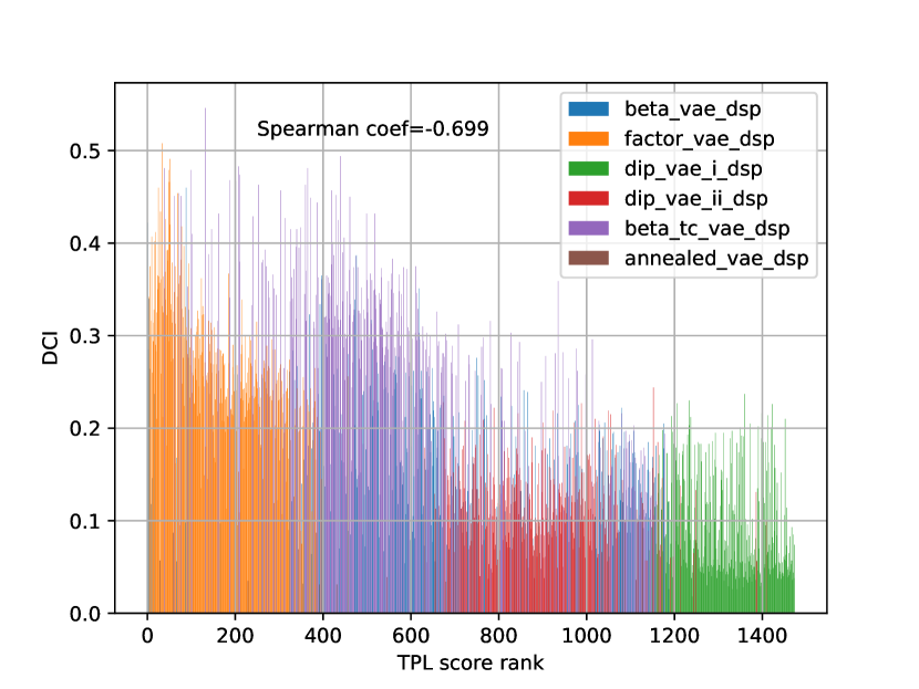
Figure 53: TPL (act$>$3) vs DCI. Ranked by TPL scores.

Figure 54: TPL (act$>$3) vs BVM. Ranked by TPL scores.

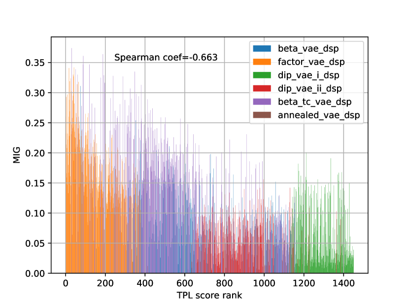
Figure 55: TPL (act$>$4) vs MIG. Ranked by TPL scores.

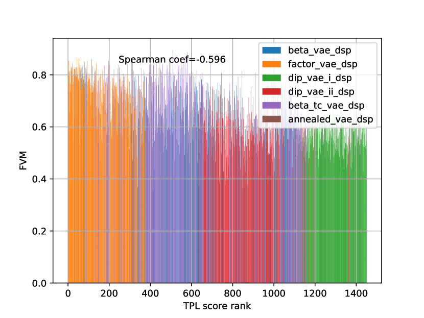
Figure 56: TPL (act$>$4) vs FVM. Ranked by TPL scores.

Figure 57: TPL (act$>$4) vs DCI. Ranked by TPL scores.

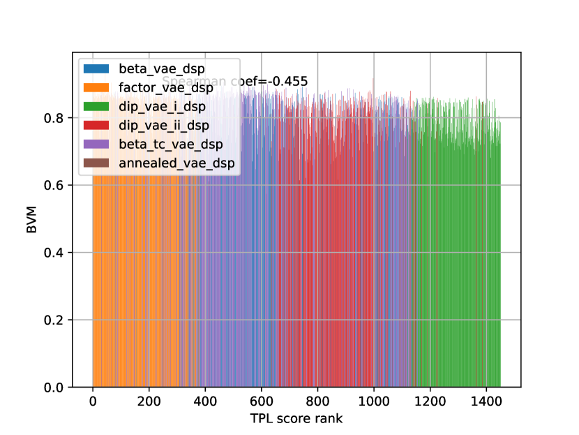
Figure 58: TPL (act$>$4) vs BVM. Ranked by TPL scores.

11 Ablation Study on the Number of Rectangles $J$

We show the impact of the number of rectangles used in our SC modules on the CelebA dataset. We vary $J$ from 1 to 9 while keeping all other factors unchanged. The results are shown in Table 6. We can see using too few rectangles harms FID (variation controlled by each code is too simple) while using too many harms TPL (each code controls entangled variations). A balanced $J$ is about 3$\sim$6.

$J$	TPL	PPL	FID
1	5.4	29.2	9.0
3	7.0	35.8	7.7
4	7.1	38.4	5.9
6	8.1	38.9	6.0
9	8.2	40.0	6.2

Table 6: Ablation on $J$ on CelebA dataset.

12 More Qualitative Results

More traversals are shown in Fig. 59 - Fig. 70. For Clevr-Complex, we can see our model learns the position concepts for both objects, but other concepts like size and shape of objects are still entangled. This indicates the multi-object disentangled representation learning is still a hard and unsolved problem.

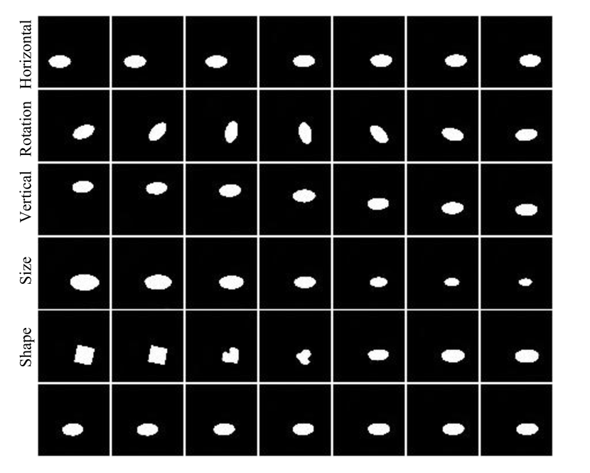
Figure 59: DSprites 1.

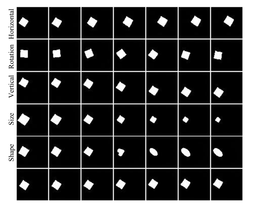
Figure 60: DSprites 2.

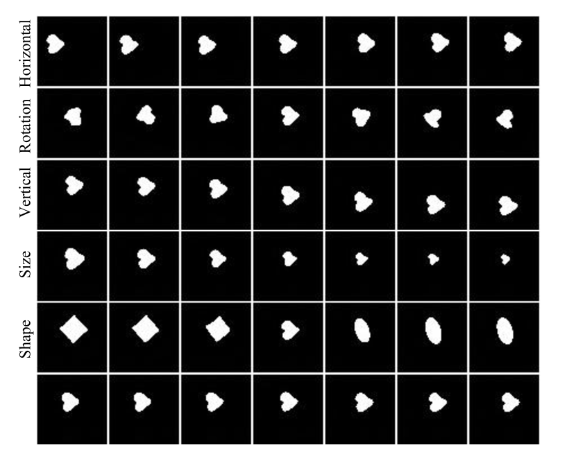
Figure 61: DSprites 3.

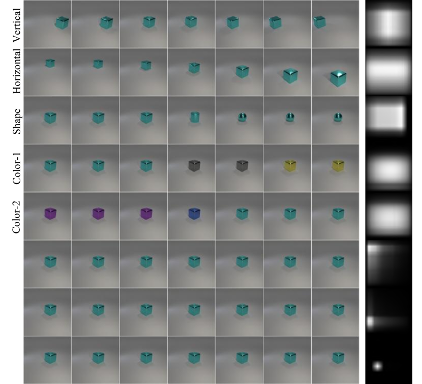
Figure 62: Clevr-Simple 1.

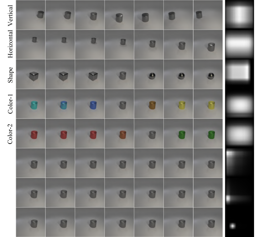
Figure 63: Clevr-Simple 2.

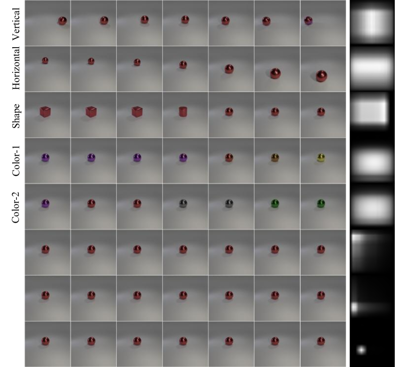
Figure 64: Clevr-Simple 3.

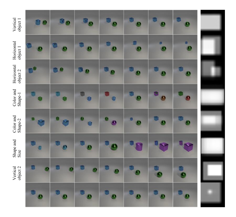
Figure 65: Clevr-Complex 1.

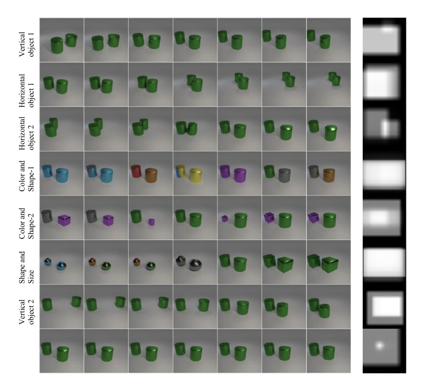
Figure 66: Clevr-Complex 2.

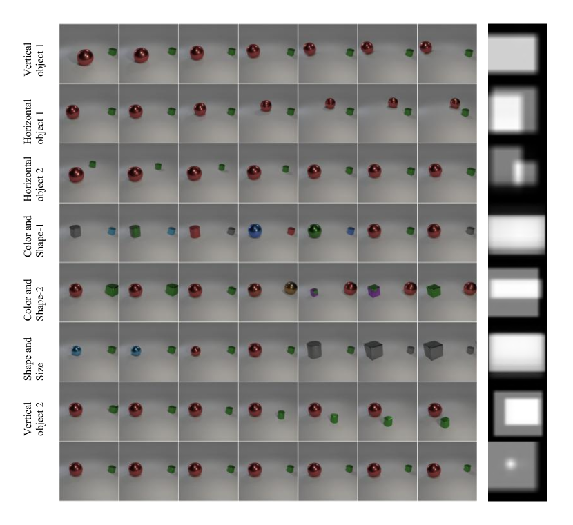
Figure 67: Clevr-Complex 3.

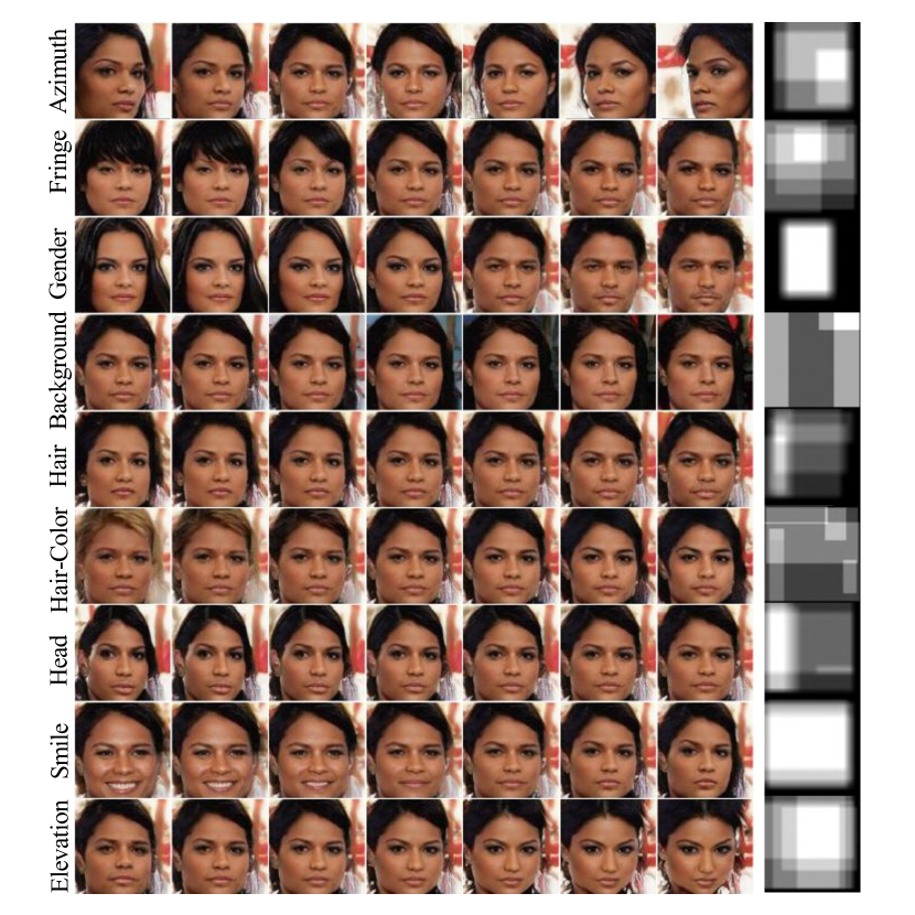
Figure 68: CelebA 1.

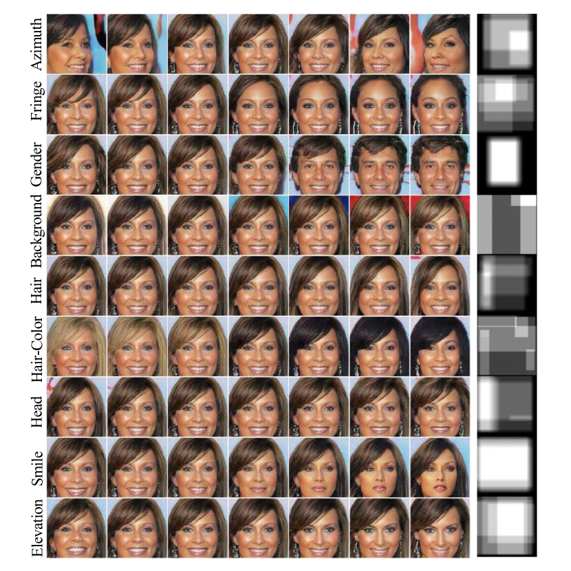
Figure 69: CelebA 2.

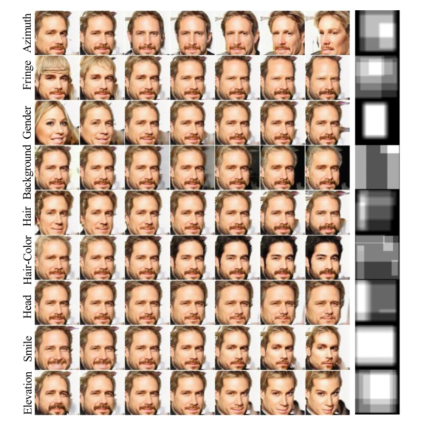
Figure 70: CelebA 3.

13 More Image Editing

More image editing experiments (similar to Fig. 10) are shown in Fig. 71 and Fig. 72. We can see the attributes of background, azimuth, smile, hat, fringe, skin color are successfully disentangled in the learned representation. However, there are still some flaws, such as the transfer of hat in the last row of Fig. 72 changes the style and color of hats in the resulting images. This problem may be caused by the lack of data of various hats during training, but may also be alleviated by better models.

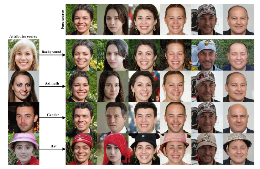
Figure 71: Image editing by transferring attributes.

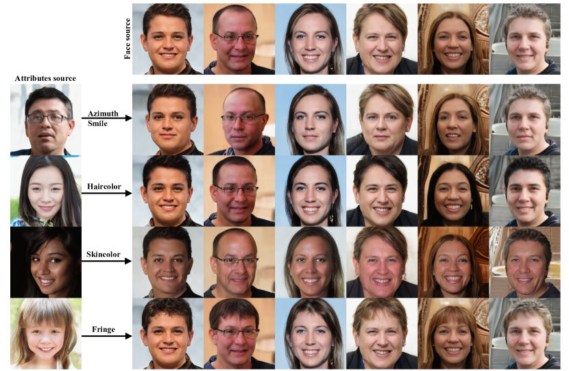
Figure 72: Image editing by transferring attributes.

14 Implementations

The network architectures are shown in multiple Tables: on CelebA: 7, 8, 9; on Shoes+Edges: 10, 11, 12; on Clevr-Simple and Clevr-Complex: 13, 14, 15; on FFHQ: 16, 17, 18; on DSprites: 19, 20, 21; on 3DShapes: 22, 23, 24; All models are trained with the Adam optimizer. For both generator and discriminator optimizers, $\beta_{1}=0$, $\beta_{2}=0.99$, initial learning rate is 0.002, except for 3DShapes we set 0.005. Note that the $Q$ network is trained together with the generator. The $\lambda$ for Shoes+Edges, Clevr-Complex, CelebA, FFHQ is 0.01, for Clevr-Simple is 0.05, for DSprites and 3DShapes is 0.001. The $p_{\text{var}}$ is 0.2 for DSprites and 3DShapes, and is 1 for other datasets. For CelebA dataset, models are trained for 4,000k images (around 19 epochs). For FFHQ dataset, models are trained until FID starts to saturate (around 28 epochs). For DSprites dataset, models are trained for 15,000k images (around 20 epochs). For 3DShapes dataset, models are trained for 8,000k images (around 18 epochs). For DSprites and 3DShapes, instead of randomly sampling the perturbed dimension $k$ in the PC loss every iteration, we loop the $k$ sequentially for each dimension every 1k images to achieve a stabler convergence.

Layer	Out Shape
Const	4x4x512
ResConv-up-1	8x8x512
SC-4-5	8x8x512
ResConv-id-1	8x8x512
Noise-2	8x8x512
ResConv-up-1	16x16x512
SC-6-5	16x16x512
ResConv-id-1	16x16x512
Noise-2	16x16x512
ResConv-up-1	32x32x512
SC-6-5	32x32x512
ResConv-id-1	32x32x512
Noise-2	32x32x256
ResConv-up-1	64x64x256
SC-6-5	64x64x256
ResConv-id-1	64x64x256
Noise-2	64x64x256
ResConv-up-1	128x128x256
SC-4-5	128x128x256
ResConv-id-1	128x128x128
Noise-2	128x128x128
ResConv-id-2	128x128x128
ResConv-id-1	128x128x3

Table 7: Generator on CelebA.

Layer	Out Shape
ResConv-down-2	128x128x64
ResConv-down-2	64x64x64
ResConv-down-2	32x32x128
ResConv-down-2	16x16x256
ResConv-down-2	8x8x512
ResConv-down-2	4x4x512
Conv-id-1	4x4x512
Dense-1	1

Table 8: Discriminator on CelebA.

Layer	Out Shape
ResConv-down-2	256x256x64
ResConv-down-2	128x128x64
ResConv-down-2	64x64x64
ResConv-down-2	32x32x128
ResConv-down-2	16x16x256
ResConv-down-2	8x8x512
ResConv-down-2	4x4x512
Conv-id-1	4x4x512
Dense-1	25

Table 9: Recognizer $Q$ on CelebA.

Layer	Out Shape
Const	4x4x512
ResConv-up-1	8x8x512
SC-4-3	8x8x512
ResConv-id-1	8x8x512
Noise-2	8x8x512
ResConv-up-1	16x16x512
SC-6-3	16x16x512
ResConv-id-1	16x16x256
Noise-2	16x16x256
ResConv-up-1	32x32x256
SC-6-3	32x32x256
ResConv-id-1	32x32x256
Noise-2	32x32x128
ResConv-up-1	64x64x128
SC-6-3	64x64x128
ResConv-id-1	64x64x128
Noise-2	64x64x128
ResConv-up-1	128x128x128
SC-4-3	128x128x128
ResConv-id-1	128x128x64
Noise-2	128x128x64
ResConv-id-2	128x128x64
ResConv-id-1	128x128x3

Table 10: Generator on Shoes+Edges.

Layer	Out Shape
ResConv-down-2	128x128x64
ResConv-down-2	64x64x64
ResConv-down-2	32x32x64
ResConv-down-2	16x16x128
ResConv-down-2	8x8x256
ResConv-down-2	4x4x512
Conv-id-1	4x4x512
Dense-1	1

Table 11: Discriminator on Shoes+Edges.

Layer	Out Shape
ResConv-down-2	128x128x64
ResConv-down-2	64x64x64
ResConv-down-2	32x32x64
ResConv-down-2	16x16x128
ResConv-down-2	8x8x256
ResConv-down-2	4x4x512
Conv-id-1	4x4x512
Dense-1	15

Table 12: Recognizer $Q$ on Shoes+Edges.

Layer	Out Shape
Const	4x4x512
ResConv-up-1	8x8x512
SC-1-2	8x8x512
Noise-1	8x8x512
ResConv-up-1	16x16x512
SC-1-2	16x16x512
Noise-1	16x16x256
ResConv-up-1	32x32x256
SC-1-2	32x32x256
Noise-1	32x32x256
ResConv-up-1	64x64x128
SC-1-2	64x64x128
Noise-1	64x64x128
ResConv-up-1	128x128x128
SC-1-2	128x128x128
Noise-1	128x128x64
ResConv-up-1	256x256x64
Noise-1	256x256x64
ResConv-id-1	256x256x3

Table 13: Generator on Clevr-Simple and -Complex.

Layer	Out Shape
ResConv-down-2	256x256x64
ResConv-down-2	128x128x64
ResConv-down-2	64x64x64
ResConv-down-2	32x32x64
ResConv-down-2	16x16x128
ResConv-down-2	8x8x256
ResConv-down-2	4x4x512
Conv-id-1	4x4x512
Dense-1	1

Table 14: Discriminator on Clevr-Simple and -Complex.

Layer	Out Shape
ResConv-down-2	256x256x64
ResConv-down-2	128x128x64
ResConv-down-2	64x64x64
ResConv-down-2	32x32x64
ResConv-down-2	16x16x128
ResConv-down-2	8x8x256
ResConv-down-2	4x4x512
Conv-id-1	4x4x512
Dense-1	10

Table 15: Recognizer $Q$ on Clevr-Simple and -Complex.

Layer	Out Shape
Const	4x4x512
ResConv-up-1	8x8x512
SC-4-5	8x8x512
ResConv-id-1	8x8x512
Noise-2	8x8x512
ResConv-up-1	16x16x512
SC-4-5	16x16x512
ResConv-id-1	16x16x512
Noise-2	16x16x512
ResConv-up-1	32x32x512
SC-4-5	32x32x512
ResConv-id-1	32x32x512
Noise-2	32x32x256
ResConv-up-1	64x64x256
SC-4-5	64x64x256
ResConv-id-1	64x64x256
Noise-2	64x64x256
ResConv-up-1	128x128x256
SC-4-5	128x128x256
ResConv-id-1	128x128x128
Noise-2	128x128x128
ResConv-up-1	256x256x128
SC-4-5	256x256x128
ResConv-id-1	256x256x128
Noise-2	256x256x64
ResConv-id-1	256x256x64
ResConv-up-1	512x512x64
ResConv-id-2	512x512x64
ResConv-id-1	512x512x3

Table 16: Generator on FFHQ.

Layer	Out Shape
ResConv-down-2	256x256x64
ResConv-down-2	128x128x64
ResConv-down-2	64x64x64
ResConv-down-2	32x32x128
ResConv-down-2	16x16x256
ResConv-down-2	8x8x512
ResConv-down-2	4x4x512
Conv-id-1	4x4x512
Dense-1	1

Table 17: Discriminator on FFHQ.

Layer	Out Shape
ResConv-down-2	256x256x64
ResConv-down-2	128x128x64
ResConv-down-2	64x64x64
ResConv-down-2	32x32x128
ResConv-down-2	16x16x256
ResConv-down-2	8x8x512
ResConv-down-2	4x4x512
Conv-id-1	4x4x512
Dense-1	30

Table 18: Recognizer $Q$ on FFHQ.

Layer	Out Shape
Const	4x4x512
AdaIN-1	4x4x128
Conv-id-1	4x4x128
AdaIN-1	4x4x128
Conv-id-1	4x4x64
AdaIN-1	4x4x64
Conv-up-1	8x8x64
AdaIN-1	8x8x64
Conv-id-1	8x8x32
AdaIN-1	8x8x32
Conv-id-1	8x8x32
AdaIN-1	8x8x32
Conv-up-1	16x16x16
AdaIN-1	16x16x16
Conv-id-1	16x16x16
AdaIN-1	16x16x16
Conv-id-1	16x16x16
AdaIN-1	16x16x16
Conv-up-1	32x32x16
Conv-id-1	32x32x16
Conv-up-1	64x64x16
Conv-id-1	64x64x1

Table 19: Generator on DSprites.

Layer	Out Shape
ResConv-down-2	64x64x16
ResConv-down-2	32x32x16
ResConv-down-2	16x16x32
ResConv-down-2	8x8x64
ResConv-down-2	4x4x128
Conv-id-1	4x4x128
Dense-1	1

Table 20: Discriminator on DSprites.

Layer	Out Shape
ResConv-down-2	64x64x16
ResConv-down-2	32x32x16
ResConv-down-2	16x16x16
ResConv-down-2	8x8x16
ResConv-down-2	4x4x32
Conv-id-1	4x4x32
Dense-1	9

Table 21: Recognizer $Q$ on DSprites.

Layer	Out Shape
Const	4x4x512
Conv-up-1	8x8x256
SC-3-2	8x8x256
ResConv-id-1	8x8x256
SC-4-3	8x8x256
ResConv-id-1	8x8x128
Conv-up-1	16x16x128
SC-4-3	16x16x128
ResConv-id-1	16x16x64
SC-4-3	16x16x64
ResConv-id-1	16x16x64
Conv-up-1	32x32x64
ResConv-id-1	32x32x32
Conv-up-1	64x64x32
ResConv-id-1	64x64x32
Conv-id-1	64x64x3

Table 22: Generator on 3DShapes.

Layer	Out Shape
ResConv-down-2	64x64x32
ResConv-down-2	32x32x32
ResConv-down-2	16x16x32
ResConv-down-2	8x8x64
ResConv-down-2	4x4x128
Conv-id-1	4x4x128
Dense-1	1

Table 23: Discriminator on 3DShapes.

Layer	Out Shape
ResConv-down-2	64x64x32
ResConv-down-2	32x32x32
ResConv-down-2	16x16x32
ResConv-down-2	8x8x64
ResConv-down-2	4x4x128
Conv-id-1	4x4x128
Dense-1	12

Table 24: Recognizer $Q$ on 3DShapes.

References

- [1] David Bau, Jun-Yan Zhu, Hendrik Strobelt, Bolei Zhou, Joshua B. Tenenbaum, William T. Freeman, and Antonio Torralba. Gan dissection: Visualizing and understanding generative adversarial networks. In Proceedings of the International Conference on Learning Representations (ICLR), 2019.
- [2] Yoshua Bengio, Aaron C. Courville, and Pascal Vincent. Representation learning: A review and new perspectives. IEEE Transactions on Pattern Analysis and Machine Intelligence, 35:1798–1828, 2012.
- [3] Diane Bouchacourt, Ryota Tomioka, and Sebastian Nowozin. Multi-level variational autoencoder: Learning disentangled representations from grouped observations. In AAAI, 2018.
- [4] Christopher P. Burgess, Irina Higgins, Arka Pal, Loïc Matthey, Nick Watters, Guillaume Desjardins, and Alexander Lerchner. Understanding disentangling in beta-vae. ArXiv, abs/1804.03599, 2018.
- [5] Jinming Cao, Oren Katzir, Peng Jiang, Dani Lischinski, Daniel Cohen-Or, Changhe Tu, and Yangyan Li. Dida: Disentangled synthesis for domain adaptation. ArXiv, abs/1805.08019, 2018.
- [6] Yue Cao, Jiarui Xu, Stephen Lin, Fangyun Wei, and Han Hu. Gcnet: Non-local networks meet squeeze-excitation networks and beyond. 2019 IEEE/CVF International Conference on Computer Vision Workshop (ICCVW), pages 1971–1980, 2019.
- [7] Ricky T. Q. Chen, Xuechen Li, Roger Grosse, and David Duvenaud. Isolating sources of disentanglement in variational autoencoders. In Advances in Neural Information Processing Systems, 2018.
- [8] Xi Chen, Yan Duan, Rein Houthooft, John Schulman, Ilya Sutskever, and Pieter Abbeel. Infogan: Interpretable representation learning by information maximizing generative adversarial nets. In NIPS, 2016.
- [9] Elliot Creager, David Madras, Jörn-Henrik Jacobsen, Marissa A. Weis, Kevin Swersky, Toniann Pitassi, and Richard S. Zemel. Flexibly fair representation learning by disentanglement. In ICML, 2019.
- [10] Kien Do and Truyen Tran. Theory and evaluation metrics for learning disentangled representations. In International Conference on Learning Representations, 2020.
- [11] Alexey Dosovitskiy, Jost Tobias Springenberg, and Thomas Brox. Learning to generate chairs with convolutional neural networks. 2015 IEEE Conference on Computer Vision and Pattern Recognition (CVPR), pages 1538–1546, 2014.
- [12] Sunny Duan, Nicholas Watters, Loic Matthey, Christopher P. Burgess, Alexander Lerchner, and Irina Higgins. Unsupervised model selection for variational disentangled representation learning. ICLR, 2020.
- [13] Emilien Dupont. Learning disentangled joint continuous and discrete representations. In NeurIPS, 2018.
- [14] Cian Eastwood and Christopher K. I. Williams. A framework for the quantitative evaluation of disentangled representations. In ICLR, 2018.
- [15] Leon A. Gatys, Alexander S. Ecker, and Matthias Bethge. Image style transfer using convolutional neural networks. 2016 IEEE Conference on Computer Vision and Pattern Recognition (CVPR), pages 2414–2423, 2016.
- [16] Ian J. Goodfellow, Jean Pouget-Abadie, Mehdi Mirza, Bing Xu, David Warde-Farley, Sherjil Ozair, Aaron C. Courville, and Yoshua Bengio. Generative adversarial networks. In NIPS, 2014.
- [17] Martin Heusel, Hubert Ramsauer, Thomas Unterthiner, Bernhard Nessler, and Sepp Hochreiter. Gans trained by a two time-scale update rule converge to a local nash equilibrium. In NIPS, 2017.
- [18] Irina Higgins, Loïc Matthey, Arka Pal, Christopher Burgess, Xavier Glorot, Matthew M Botvinick, Shakir Mohamed, and Alexander Lerchner. beta-vae: Learning basic visual concepts with a constrained variational framework. In ICLR, 2017.
- [19] Haruo Hosoya. Group-based learning of disentangled representations with generalizability for novel contents. In IJCAI, 2019.
- [20] Xun Huang and Serge J. Belongie. Arbitrary style transfer in real-time with adaptive instance normalization. 2017 IEEE International Conference on Computer Vision (ICCV), pages 1510–1519, 2017.
- [21] Insu Jeon, Wonkwang Lee, and Gunhee Kim. Ib-gan: Disentangled representation learning with information bottleneck gan. ArXiv, 2018.
- [22] Yeonwoo Jeong and Hyun Oh Song. Learning discrete and continuous factors of data via alternating disentanglement. In ICML, 2019.
- [23] J. Johnson, B. Hariharan, L. van der Maaten, L. Fei-Fei, C. L. Zitnick, and R. Girshick. Clevr: A diagnostic dataset for compositional language and elementary visual reasoning. In 2017 IEEE Conference on Computer Vision and Pattern Recognition (CVPR), pages 1988–1997, 2017.
- [24] Tero Karras, Timo Aila, Samuli Laine, and Jaakko Lehtinen. Progressive growing of GANs for improved quality, stability, and variation. In International Conference on Learning Representations, 2018.
- [25] Tero Karras, Samuli Laine, and Timo Aila. A style-based generator architecture for generative adversarial networks. IEEE transactions on pattern analysis and machine intelligence, 2020.
- [26] Tero Karras, Samuli Laine, Miika Aittala, Janne Hellsten, Jaakko Lehtinen, and Timo Aila. Analyzing and improving the image quality of stylegan. 2019.
- [27] Tero Karras, Samuli Laine, Miika Aittala, Janne Hellsten, Jaakko Lehtinen, and Timo Aila. Analyzing and improving the image quality of stylegan. CVPR, 2020.
- [28] Hadi Kazemi, Seyed Mehdi Iranmanesh, and Nasser M. Nasrabadi. Style and content disentanglement in generative adversarial networks. 2019 IEEE Winter Conference on Applications of Computer Vision (WACV), pages 848–856, 2019.
- [29] Hyunjik Kim and Andriy Mnih. Disentangling by factorising. In ICML, 2018.
- [30] Diederik P. Kingma, Shakir Mohamed, Danilo Jimenez Rezende, and Max Welling. Semi-supervised learning with deep generative models. In NIPS, 2014.
- [31] Diederik P. Kingma and Max Welling. Auto-encoding variational bayes. In ICLR, 2013.
- [32] Tejas D. Kulkarni, William F. Whitney, Pushmeet Kohli, and Joshua B. Tenenbaum. Deep convolutional inverse graphics network. In NIPS, 2015.
- [33] Abhishek Kumar, Prasanna Sattigeri, and Avinash Balakrishnan. Variational inference of disentangled latent concepts from unlabeled observations. In ICLR, 2018.
- [34] Guillaume Lample, Neil Zeghidour, Nicolas Usunier, Antoine Bordes, Ludovic Denoyer, and Marc’Aurelio Ranzato. Fader networks: Manipulating images by sliding attributes. In NIPS, volume abs/1706.00409, 2017.
- [35] Hsin-Ying Lee, Hung-Yu Tseng, Jia-Bin Huang, Maneesh Kumar Singh, and Ming-Hsuan Yang. Diverse image-to-image translation via disentangled representations. ECCV, abs/1808.00948, 2018.
- [36] Lingzhi Li, Jianmin Bao, Hao Yang, Dong Chen, and Fang Wen. Advancing high fidelity identity swapping for forgery detection. In Proceedings of the IEEE/CVF Conference on Computer Vision and Pattern Recognition (CVPR), June 2020.
- [37] Zhiyuan Li, Jaideep Vitthal Murkute, Prashnna Kumar Gyawali, and Lin-Wei Wang. Progressive learning and disentanglement of hierarchical representations. ICLR, abs/2002.10549, 2020.
- [38] Zinan Lin, Kiran Koshy Thekumparampil, Giulia Fanti, and Sewoong Oh. Infogan-cr: Disentangling generative adversarial networks with contrastive regularizers. ICML, 2020.
- [39] Ziwei Liu, Ping Luo, Xiaogang Wang, and Xiaoou Tang. Deep learning face attributes in the wild. 2015 IEEE International Conference on Computer Vision (ICCV), pages 3730–3738, 2014.
- [40] Francesco Locatello, Gabriele Abbati, Tom Rainforth, Stefan Bauer, Bernhard Schölkopf, and Olivier Bachem. On the fairness of disentangled representations. In NeurIPS, 2019.
- [41] Francesco Locatello, Stefan Bauer, Mario Lucic, Gunnar Rätsch, Sylvain Gelly, Bernhard Schölkopf, and Olivier Bachem. Challenging common assumptions in the unsupervised learning of disentangled representations. In ICML, 2019.
- [42] Francesco Locatello, Ben Poole, Gunnar Ratsch, Bernhard Scholkopf, Olivier Bachem, and Michael Tschannen. Weakly-supervised disentanglement without compromises. ArXiv, abs/2002.02886, 2020.
- [43] Francesco Locatello, Michael Tschannen, Stefan Bauer, Gunnar Rätsch, Bernhard Schölkopf, and Olivier Bachem. Disentangling factors of variations using few labels. In International Conference on Learning Representations, 2020.
- [44] Emile Mathieu, Tom Rainforth, Nana Siddharth, and Yee Whye Teh. Disentangling disentanglement in variational autoencoders. In ICML, 2018.
- [45] William Peebles, John Peebles, Jun-Yan Zhu, Alexei A. Efros, and Antonio Torralba. The hessian penalty: A weak prior for unsupervised disentanglement. In Proceedings of European Conference on Computer Vision (ECCV), 2020.
- [46] Xingchao Peng, Zijun Huang, Ximeng Sun, and Kate Saenko. Domain agnostic learning with disentangled representations. In ICML, 2019.
- [47] Scott E. Reed, Kihyuk Sohn, Yuting Zhang, and Honglak Lee. Learning to disentangle factors of variation with manifold interaction. In ICML, 2014.
- [48] Yikang Shen, Shawn Tan, Alessandro Sordoni, and Aaron C. Courville. Ordered neurons: Integrating tree structures into recurrent neural networks. ArXiv, abs/1810.09536, 2019.
- [49] Karen Simonyan and Andrew Zisserman. Very deep convolutional networks for large-scale image recognition. In International Conference on Learning Representations, 2015.
- [50] Krishna Kumar Singh, Utkarsh Ojha, and Yong Jae Lee. Finegan: Unsupervised hierarchical disentanglement for fine-grained object generation and discovery. In CVPR, 2019.
- [51] Luan Tran, Xi Yin, and Xiaoming Liu. Disentangled representation learning gan for pose-invariant face recognition. 2017 IEEE Conference on Computer Vision and Pattern Recognition (CVPR), pages 1283–1292, 2017.
- [52] Dmitry Ulyanov, Vadim Lebedev, Andrea Vedaldi, and Victor S. Lempitsky. Texture networks: Feed-forward synthesis of textures and stylized images. In ICML, 2016.
- [53] Dmitry Ulyanov, Andrea Vedaldi, and Victor S. Lempitsky. Improved texture networks: Maximizing quality and diversity in feed-forward stylization and texture synthesis. 2017 IEEE Conference on Computer Vision and Pattern Recognition (CVPR), pages 4105–4113, 2017.
- [54] Sjoerd van Steenkiste, Francesco Locatello, Jurgen Schmidhuber, and Olivier Bachem. Are disentangled representations helpful for abstract visual reasoning? In NIPS, 2019.
- [55] Ashish Vaswani, Noam Shazeer, Niki Parmar, Jakob Uszkoreit, Llion Jones, Aidan N. Gomez, Lukasz Kaiser, and Illia Polosukhin. Attention is all you need. NIPS, abs/1706.03762, 2017.
- [56] Xianglei Xing, Tian Han, Ruiqi Gao, Song-Chun Zhu, and Ying Nian Wu. Unsupervised disentangling of appearance and geometry by deformable generator network. 2019 IEEE/CVF Conference on Computer Vision and Pattern Recognition (CVPR), pages 10346–10355, 2019.
- [57] Xinchen Yan, Jimei Yang, Kihyuk Sohn, and Honglak Lee. Attribute2image: Conditional image generation from visual attributes. In ECCV, 2016.
- [58] A. Yu and K. Grauman. Fine-grained visual comparisons with local learning. In Computer Vision and Pattern Recognition (CVPR), Jun 2014.
- [59] Shengjia Zhao, Jiaming Song, and Stefano Ermon. Learning hierarchical features from generative models. In ICML, 2017.
- [60] Xinqi Zhu, Chang Xu, and Dacheng Tao. Learning disentangled representations with latent variation predictability. In ECCV, 2020.