A Framework for Generalized Benders’ Decomposition and Its Application to Multilevel Optimization

Abstract

We describe a framework for reformulating and solving optimization problems that generalizes the well-known framework originally introduced by Benders. We discuss details of the application of the procedures to several classes of optimization problems that fall under the umbrella of multilevel/multistage mixed integer linear optimization problems. The application of this abstract framework to this broad class of problems provides new insights and a broader interpretation of the core ideas, especially as they relate to duality and the value functions of optimization problems that arise in this context.

1 Introduction

This paper describes a framework for reformulating and solving optimization problems that extends the well-known framework of Benders [1962]. Although the basic elements of the framework are known, we provide a self-contained development of the key concepts and illustrate in detail the principles involved by applying them to the solution of several classes of optimization problems, including one to which they have not previously been applied. These classes of problems are all contained under the broad umbrella of what we informally refer to as multilevel/multistage mixed integer linear optimization problems (MMILPs). MMILPs comprise a broad class of optimization problems in which multiple decision makers (DMs), with possibly competing objectives, make decisions in sequence over time. Each DM’s decision impacts the options available to other DMs at other (typically later) stages. In economics, these problems fall under the general umbrella of game theory. We do not formally define the broad class comprising MMILPs here, but rather describe some specific subclasses contained within it. Readers wishing to have a more complete overview of MMILPs should refer to Bolusani et al. [2020].

Although Benders’ technique was originally applied to standard mathematical optimization problems with an underlying structure suggesting a partition of the variables into exactly two sets, it can be similarly applied not only to more general classes of optimization problems, but by extension, to $l$-stage problems in which there is an obvious division of the variables into $l$ sets. Because an $l$-stage MMILP is most naturally defined recursively in terms of an ($l-1$)-stage MMILP, the very structure of MMILPs seems to suggest solution by an approach similar to the one suggested by Benders. The recursive structure also mirrors that of the polynomial time hierarchy (PTH, originally introduced by Stockmeyer [1976]), a recursively defined family of complexity classes into which MMILPs can naturally be categorized. The lowest level of the PTH is the well-known class ${\mathsf{P}}$ of problems solvable in time polynomial in the size of the input, and the $l^{\textrm{th}}$ level (whose class of primary interest is denoted $\Sigma_{l}^{P}$) is comprised of problems solvable in polynomial time given an oracle for problems in the $(l-1)^{\textrm{st}}$ level. The decision versions of MMILPs with $l$ levels are prototypical complete problems for $\Sigma_{l}^{P}$ [Jeroslow, 1985], meaning that all other problems in the class can be reduced to MMILPs.

Benders’ framework is, first and foremost, a technique for reformulation. Using this technique, MMILPs can be recast as standard mathematical optimization problems. The reformulation usually results in an exponential increase in size relative to the original formulation, and a number of additional transformations may be necessary to get the final problem into a form in which a blackbox solver can digest it. Because of the exponential increase in size, the reformulation must generally be solved either by an approach based on a convergent iterative approximation scheme or by utilizing a relaxation to obtain bounds that can then be used to drive a branch-and-bound algorithm. These two approaches are closely related, as the relaxations required in the latter approach can be obtained by terminating the iterative approximation procedure before convergence. We further discuss approaches based on branch and bound in Section 2.3.

In the remainder of the paper, we focus only on the iterative approximation approach, which can be seen as a generalization of the cutting-plane method for solving mixed integer linear optimization problems (MILPs). This approach can be applied recursively, essentially decomposing the problem by stage, with the subproblem (introduced formally in Section 2) that arises when solving an $l$-stage problem being an (lexicographic) optimization problem with $l-1$ stages. The main contributions of this work are (1) the development of an abstract framework for generalizing the principles of Benders’ technique for reformulation that encompasses non-traditional problem classes, (2) the specification of an associated algorithmic procedure that generalizes the standard cutting-plane algorithm and is based on iterative approximation of functions arising from the projection of the original problem into the space of a specified subset of variables, and (3) its application to the solution of mixed integer two-stage/bilevel linear optimization problems (MIBLPs). To our knowledge, this is the first algorithm for MIBLPs that utilizes a generalized Benders’ approach. This paper does not aim at discussing efficiency or comparing the algorithms described herein to alternatives. While we have implemented a proof-of-concept for the algorithms described here, a full-featured, efficient implementation would require substantial additional development.

The paper is organized as follows. In Section 2, we discuss the principles underlying our generalized Benders’ framework at a high level in the context of a general optimization problem, including concepts of bounding functions and general duality. We also highlight the relationships between this framework and certain existing algorithms at an abstract level. In Section 3, we illustrate these principles concretely with two examples, summarizing existing algorithms for the case in which there are two stages and the objective functions are the same in both stages. Section 4 goes into more detail in describing an algorithm for general MIBLPs, the special case of MMILPs in which there are only two stages. Finally, we conclude in Section 5 by briefly discussing a conceptual extension of the algorithm for MIBLPs to general MMILPs with $l$ stages.

2 Benders’ Principle

In this section, we introduce the basic principles of the framework. We first describe it in a very general context and then focus on the special case in which the objective and constraint functions are additively separable. The idea of such a generalization of Benders’ original algorithm is not new. As far back as the 1970s, Geoffrion [1972] had already proposed a similar idea. Its application to MMILPs, however, provides new insights and broader interpretations of the core ideas.

What we generally mean by a Benders-type approach is a technique for reformulation and/or solution of an optimization problem that operates in a subspace associated with a specified subset of variables from the original compact formulation. We refer to this subset of variables as the first-stage variables throughout the paper, although Benders’ technique only really provides a separation of the problem into independent “stages” once we assume additive separability. The essential element underlying any Benders-type method is a projection operation. Projecting an optimization problem means projecting both its feasible region and its objective function, in the fashion we describe, in order to obtain a valid reformulation involving only first-stage variables. By “valid reformulation,” we mean one in which the set of optimal solutions of the projected problem is the projection of the set of optimal solutions of the original problem, though one could define the concept of validity in other ways.

The projection operation is natural in applications where the optimal values of the first-stage variables are of primary concern, while the remaining variables are present only to model the later-stage effects of the first-stage decisions. The goal of the projection operation, however, is purely pragmatic—it is to construct a reformulation that is somehow algorithmically advantageous. The advantage may either be because the associated relaxations are more effective or simply because the reformulation has a form that makes the employment of existing blackbox solvers easier. The reformulation process necessarily introduces complex functions of the first-stage variables, which model the effects mentioned above. Algorithms for solving these reformulations generally construct approximations of these functions, as we detail in the following sections.

2.1 General Optimization Problems

We first consider the following very general form of optimization problem in which the variables are partitioned into two sets, the first- and second-stage variables, denoted by $x\in\mathbb{R}^{n_{1}}$ and $y\in\mathbb{R}^{n_{2}}$, respectively. The problem is then

$$\min\limits_{x\in X,\ y\in Y}\left\{f(x,y)\;\middle|\;F(x,y)\geq 0\right\},$$ (1)

where $f:\mathbb{R}^{n_{1}}\times\mathbb{R}^{n_{2}}\rightarrow\mathbb{R}$ is the objective function and $F:\mathbb{R}^{n_{1}}\times\mathbb{R}^{n_{2}}\rightarrow\mathbb{R}^{m}$ is the constraint function, with $X\subseteq\mathbb{R}_{+}^{n_{1}}$ and $Y\subseteq\mathbb{R}_{+}^{n_{2}}$ denoting the additional disjunctive constraints on the values of the variables. Typically, we have $X=\mathbb{Z}^{r_{1}}_{+}\times\mathbb{R}^{n_{1}-r_{1}}_{+}$ and $Y=\mathbb{Z}^{r_{2}}_{+}\times\mathbb{R}^{n_{2}-r_{2}}_{+}$, and we therefore consider that form of sets for the remainder of the paper. By convention, we take the optimal objective value to be $\infty$ if the feasible region

$$\mathcal{F}=\left\{(x,y)\in X\times Y\;\middle|\;F(x,y)\geq 0\right\}$$

is empty and $-\infty$ if the problem (1) is unbounded. We assume that in all other cases, the problem has a finite minimum that can be attained.

2.1.1 Projection and the Subproblem

The simple yet fundamental idea is that (1) can be equivalently formulated as

$$\min\limits_{x\in X}\left\{\min\limits_{y\in Y}\left\{f(x,y)\;\middle|\;F(x,y)\geq 0\right\}\right\}.$$

By replacing the inner optimization problem with a function, we obtain the reformulation

$$\min\limits_{x\in X}f_{x}(x),$$ (2)

in terms of only the first-stage variables, where

$$f_{x}(x)=\min\limits_{y\in Y}\left\{f(x,y)\;\middle|\;F(x,y)\geq 0\right\}\quad\forall x\in\mathbb{R}^{n_{1}}.$$ (3)

In this new formulation, $f_{x}$ is a function that returns the objective function value of the optimal feasible combination of values for both first- and second-stage variables, given fixed values for the first-stage variables.

Although the formulation (2) does not explicitly involve projection, we define by convention that $f_{x}(x)=\infty$ if $x\not\in\operatorname{proj}_{x}(\mathcal{F})$, where

$$\operatorname{proj}_{x}(\mathcal{F})=\{x\in X\mid F(x,y)\geq 0\text{ for some }y\in Y\}$$ (4)

is the projection of the feasible region of (1) into the space of the first-stage variables. (We similarly define $f_{x}(x)=-\infty$ if the optimization problem on the right-hand side of (3) is unbounded.) This means that $f_{x}$ plays a dual role. First, it effectively prevents any first-stage solution that is not in the projected feasible region from being considered (provided the projected feasible region is non-empty). Second, it is also what we earlier described informally as the projection of the original objective function, since it ensures that the objective function value in the projected optimization problem with respect to $\hat{x}\in\operatorname{proj}_{x}(\mathcal{F})$ is exactly the value that would have been obtained if solving the original problem with the first-stage variables fixed to $\hat{x}$. Overall, the reformulation (2) can then be considered to be the projection of (1) into the space of the first-stage variables. The evaluation of $f_{x}$ for particular first-stage solutions is the aforementioned subproblem. More details about its role in the overall solution process are provided in Section 2.1.3.

2.1.2 Bounding Functions and the Master Problem

In principle, the optimal value of (1), as well as an optimal first-stage solution, can be obtained by solving (2). However, we usually do not have a closed-form description of $f_{x}$ and even when such closed form exists in theory, its description is typically of exponential size and would thus be impractical. We therefore replace $f_{x}$ in (2) with a dual bounding function $\underaccent{\bar}{f}_{x}$ (defined below) to obtain the relaxation known as the master problem.

Definition 1 (Dual Bounding Function).

A function $\underaccent{\bar}{f}_{x}:\mathbb{R}^{n_{1}}\rightarrow\mathbb{R}\cup\{\pm\infty\}$ is said to be a dual bounding function with respect to the projection of the objective function $f$ if

$$\underaccent{\bar}{f}_{x}(x)\leq f_{x}(x)\quad\forall x\in\mathbb{R}^{n_{1}}.$$

It is called strong at $\hat{x}\in X$ if

$$\underaccent{\bar}{f}_{x}(\hat{x})=f_{x}(\hat{x}).$$

Given a dual bounding function, the master problem is then

$$\min\limits_{x\in X}\underaccent{\bar}{f}_{x}(x).$$ (5)

Naturally, for any relaxation-based method to be practical, solving the relaxation (in this case, (5)) should be easier than solving the original problem (in this case, (2)). The difficulty of solving (5), however, is directly related to the structure of the function $\underaccent{\bar}{f}_{x}$ itself. In the cases discussed later, this function is piecewise linear and the master problem can be formulated as an MILP.

2.1.3 Overall Algorithm

The overall method is to iteratively improve the master problem formulation by strengthening $\underaccent{\bar}{f}_{x}$. In iteration $k$, candidate solution $x^{k}$ is generated by solving the current master problem (yielding a lower bound on the optimal value of (1)), and $f_{x}(x^{k})$ is then evaluated (yielding an upper bound on the optimal value of (1)). The algorithm alternates between solution of the master problem and the subproblem until upper and lower bounds are equal.

Although the evaluation of $f_{x}(x^{k})$ apparently involves only the determination of the optimal solution value, the solution of the subproblem also typically produces, as a byproduct, a primal-dual proof of optimality for the problem on the right-hand side of (3). It is from this primal-dual proof that we extract a dual bounding function $\underaccent{\bar}{f}_{x}^{k}$ that is strong at $x^{k}$. The form of this primal-dual proof and the structure of $\underaccent{\bar}{f}_{x}^{k}$ depends strongly on the form of the original problem. We examine particular cases in Section 2.2.2.

It is possible that an algorithm following this general outline will either converge to a local optimum or not converge at all (see Sahinidis and Grossmann [1991]), but the convergence of the method to a global optimal solution can be guaranteed under two conditions that are satisfied in many important cases. The first of these is that we update $\underaccent{\bar}{f}_{x}$ in each iteration $k$ in such a way that we guarantee that it is strong not only at $x^{k}$ but also at all $x^{i}$, $i<k$. This can be most easily accomplished by taking the maximum of the bounding functions generated at each iteration. That is, after iteration $k$,

$$\underaccent{\bar}{f}_{x}(x)=\max_{1\leq i\leq k}\underaccent{\bar}{f}_{x}^{i}(x),$$ (6)

where $\underaccent{\bar}{f}_{x}^{i}$ is the dual bounding function obtained in iteration $i\leq k$ of the algorithm. In such cases, the master problem (5) is usually reformulated using a standard trick to eliminate the maximum operator by introducing an auxiliary variable $z$ to obtain

$$\min\limits_{x\in X} \;z$$ (7)

s.t. $$\;z\geq\underaccent{\bar}{f}_{x}^{i}(x)\quad 1\leq i\leq k.$$

The formulations (7) and (5) are equivalent in this case because $z$ must be equal to the maximum of the individual bounding functions at optimality. In the literature, the constraints $z\geq\underaccent{\bar}{f}_{x}^{i}(x)$ for $1\leq i\leq k$ in (7) are sometimes called Benders’ optimality constraints. Depending on how the master problem is reformulated, it may also sometimes be necessary to explicitly exclude $x^{k}\not\in\operatorname{proj}_{x}(\mathcal{F})$ from the feasible region of the master problem, in which case the associated constraints are called Benders’ feasibility constraints.

The overall approach is outlined in Figure 1.

Generalized Benders’ Framework for Solving (1)
 Step 0. Initialize $k\leftarrow 1$, $\textrm{UB}^{0}=\infty$, $\textrm{LB}^{0}=-\infty$, $\underaccent{\bar}{f}_{x}^{0}(x)=-\infty$ for all $x\in\mathbb{R}^{n_{1}}$.
Step 1. Solve the master problem (lower bound)

• Construct the dual bounding function $\underaccent{\bar}{f}_{x}(x)=\max\limits_{0\leq i\leq k-1}\underaccent{\bar}{f}_{x}^{i}(x)$ and formulate the master problem (7).

• Solve (7) to obtain an optimal solution $(x^{k},\ z^{k})$. Set $\textrm{LB}^{k}\leftarrow z^{k}$.

Step 2. Solve the subproblem (upper bound)

• Solve (3) for the given $x^{k}$ to obtain an optimal solution $y^{k}$ and strong dual bounding function $\underaccent{\bar}{f}_{x}^{k}$ such that $\underaccent{\bar}{f}_{x}^{k}(x^{k})=f_{x}(x^{k})$. Set $\textrm{UB}^{k}\leftarrow f_{x}(x^{k})$.

• Termination check: $\textrm{UB}^{k}=\textrm{LB}^{k}$?

  1. If yes, STOP. $(x^{k},y^{k})$ is an optimal solution to (1).

  2. If no, set $k\leftarrow k+1$ and go to Step 1.

 

Figure 1: Outline of the generalized Benders’ decomposition framework

Theorem 1 due to Hooker and Ottosson [2003] shows that Algorithm 1 converges in a finite number of steps under the additional condition that $\operatorname{proj}_{x}(\mathcal{F})$ is finite.

Theorem 1 (Hooker and Ottosson [2003], Theorem 2).

If the function $\underaccent{\bar}{f}_{x}$ is defined as in (6) and $\underaccent{\bar}{f}_{x}^{i}$ is strong at $x^{i}$ in each iteration $i$, then $\underaccent{\bar}{f}_{x}$ remains a valid dual bounding function that is strong at all previous iterates and the method converges to the optimal value in a finite number of iterations under the assumption that $|\operatorname{proj}_{x}(\mathcal{F})|<\infty$.

The proof of this result is rather straightforward. In fact, a slightly more general result also holds, since the overall dual bounding function need not be constructed in this particular way, as long as we can ensure that it is strong at all the previous iterates. In practical implementations, however, taking the maximum of previous bounding functions is a natural approach and it is the one we adopt here.

This general framework still leaves many steps unspecified and raises many questions regarding implementation in specific cases. These questions will be answered in detail for the several cases of our interest in Sections 3 and 4.

2.2 Additively Separable Optimization Problems

We now move to the more specific setting that is central to the application of Benders’ method to optimization problems in which the constraint and objective functions are additively separable.

Definition 2 (Additively Separable Function).

A function $f:\mathbb{R}^{n_{1}}\times\mathbb{R}^{n_{2}}\rightarrow\mathbb{R}$ is additively separable if $\exists\;g:\mathbb{R}^{n_{1}}\rightarrow\mathbb{R}$ and $h:\mathbb{R}^{n_{2}}\rightarrow\mathbb{R}$ such that $f(x,y)=g(x)+h(y)$ for all $(x,y)\in\mathbb{R}^{n_{1}}\times\mathbb{R}^{n_{2}}$.

When the functions $f$ and $F$ are additively separable, such separability allows us to reformulate these problems in ways that enhance intuition and also ease implementation. As such, let $g:\mathbb{R}^{n_{1}}\rightarrow\mathbb{R}$, $h:\mathbb{R}^{n_{2}}\rightarrow\mathbb{R}$, $G:\mathbb{R}^{n_{1}}\rightarrow\mathbb{R}^{m}$, and $H:\mathbb{R}^{n_{2}}\rightarrow\mathbb{R}^{m}$ be such that $f(x,y)=g(x)+h(y)$ and $F(x,y)=G(x)+H(y)$ for all $(x,y)\in\mathbb{R}^{n_{1}}\times\mathbb{R}^{n_{2}}$. Because we are specifically interested in the case of linear functions, we also introduce a right-hand side $b\in\mathbb{R}^{m}$, as is standard for problems involving linear functions. We then obtain the new form of general optimization problem

$$\min\limits_{x\in X,\ y\in Y}\left\{g(x)+h(y)\;\middle|\;G(x)+H(y)\geq b\right\}$$ (8)

that we consider in the rest of the paper.

2.2.1 Projection and the Value Function

A reformulation of (8) analogous to (2), obtained upon projecting into the space of the first-stage variables, is

$$\min\limits_{x\in X}\left\{g(x)+\phi\left(b-G(x)\right)\right\},$$ (9)

where

$$\phi(\beta)=\min\limits_{y\in\mathbb{R}_{+}^{n_{2}}}\left\{h(y)\;\middle|\;y\in{\cal P}_{2}(\beta)\cap Y\right\}\quad\forall\beta\in\mathbb{R}^{m},$$ (10)

and

$$\mathcal{P}_{2}(\beta)=\left\{y\in\mathbb{R}_{+}^{n_{2}}\;\middle|\;H(y)\geq\beta\right\}\quad\forall\beta\in\mathbb{R}^{m}$$

is a parametric family of polyhedra containing points satisfying the second-stage feasibility conditions, which can now be considered fully independently, due to the additive separability. By convention, $\phi(\beta)=+\infty$ for $\beta\in\mathbb{R}^{m}$ if ${\cal P}_{2}(\beta)\cap Y=\emptyset$, and $\phi(\beta)=-\infty$ for $\beta\in\mathbb{R}^{m}$ if the problem on the right-hand side of (10) is unbounded.

As opposed to the earlier-defined function $f_{x}$, which was parameterized on the first-stage solution, $\phi$ is parameterized on the right-hand side of the associated second-stage optimization problem (which is in turn determined by the first-stage solution). The second-stage optimization problem, analogous to the earlier defined subproblem (3), is to evaluate $\phi$ at a specific right-hand side. In the context of the framework described in Figure 1, $\phi$ would be evaluated in iteration $k$ of the algorithm at the right-hand side $\beta^{k}=b-G(x^{k})$.

Those readers familiar with the more general duality theory associated with mixed integer linear optimization problems (see, e.g., Nemhauser and Wolsey [1988] and Güzelsoy and Ralphs [2007]) will recognize $\phi$ as the value function of the second-stage problem. The value function of the second-stage problem and the associated dual problem are crucial elements of the framework in the additively separable case, so we now briefly review these basic concepts.

2.2.2 General Duality and Dual Functions

The function generally referred to as “the” value function of an optimization problem is one that returns the optimal objective value for a given right-hand side vector. As in the general framework from Section 2.1, we form the master problem by replacing this value function with a function that bounds it from below. Such functions are known as dual functions, so called because they can be interpreted as solutions to a general dual problem and reflect the essential role of duality in Benders-type reformulations. For a particular right-hand side $\hat{\beta}\in\mathbb{R}^{m}$, the general dual problem

$$\max\limits_{D\in\Upsilon^{m}}\left\{D(\hat{\beta})\;\middle|\;D(\beta)\leq\phi(\beta)\quad\forall\beta\in\mathbb{R}^{m}\right\}$$ (11)

associated with (10) is an optimization problem over a class $\Upsilon^{m}\subseteq\left\{\upsilon\mid\upsilon:\mathbb{R}^{m}\rightarrow\mathbb{R}\right\}$ of real-valued functions. The objective of the dual problem is to construct a function that bounds the value function from below and for which the bound is as strong as possible at $\hat{\beta}$. As such, we define a (strong) dual function as follows.

Definition 3 (Dual Function).

A dual function $D:\mathbb{R}^{m}\rightarrow\mathbb{R}\cup\{\pm\infty\}$ is one that satisfies $D(\beta)\leq\phi(\beta)$ for all $\beta\in\mathbb{R}^{m}$. It is called strong at $\hat{\beta}\in\mathbb{R}^{m}$ if $D(\hat{\beta})=\phi(\hat{\beta})$.

The dual problem itself is called strong if $\Upsilon^{m}$ is guaranteed to contain a strong dual function. As long as the value function itself is real-valued and is a member of $\Upsilon^{m}$, then the dual problem will be strong, since the value function itself is an optimal solution of (11).

Exact solution algorithms that produce certificates of optimality typically do it by providing a primal solution, which certifies an upper bound, and a dual function (solution to (11)), which certifies a lower bound. When these bounds are equal, the combination provides the required certificate of optimality. Dual functions can be obtained in a variety of ways, but one obvious way to construct them is to consider the value function of a relaxation of the problem. Most solution algorithms for linear and mixed integer linear optimization problems work by iteratively constructing such a dual function.

The connection between the general dual and Benders’ framework should be clear. The strong dual function constructed as a certificate of optimality when solving the subproblem (evaluating $\phi$) is a function that can be directly used in strengthening the global dual function that defines the current master problem. In fact, it is useful to think of the subproblem not as that of evaluating $\phi$, but rather of solving a dual problem of the form (11) to obtain a strong dual function, which is what we actually need for forming the master problem in the next iteration.

2.2.3 Overall Algorithm

The overall method is largely similar to that described in Figure 1. We relax the reformulation (9) to obtain a master problem

$$\min\limits_{x\in X} \;g(x)+z$$ (12)

s.t. $$\;z\geq\underline{\phi}\left(b-G(x)\right),$$

in which the value function $\phi$ is replaced by a dual function $\underline{\phi}$. Solving this master problem in iteration $k$ yields a solution $(x^{k},z^{k})$ and a lower bound $g(x^{k})+z^{k}$. We then evaluate $\phi$ at $b-G(x^{k})$ to obtain a dual function $\underline{\phi}^{k}$ strong at $b-G(x^{k})$ and an upper bound $g(x^{k})+\phi(b-G(x^{k}))$. This dual function is combined with previously produced such functions to obtain a global dual function that is strong at all previous iterates, ensuring eventual convergence under the same conditions as in Theorem 1.

Naturally, the exact form and structure of the dual functions involved is crucially important to the tractability of the overall algorithm, as we do need a method of (re)formulating and solving the master problem in each iteration. In the cases discussed in this paper, the dual function takes on relatively simple forms. For linear optimization problems (LPs), the value function is convex and there is always a strong dual function that is a simple linear function. This linear function is an optimal solution to the usual LP dual, which is a subgradient of the LP value function.

In the case of mixed integer linear optimization, dual functions can be obtained as a by-product of a branch-and-bound algorithm. Roughly speaking, the lower bound produced by a branch-and-bound algorithm is the minimum of lower bounds produced for the individual subproblems associated with the leaf nodes of the branch-and-bound tree. Thus, the overall dual function is the minimum of dual functions for these subproblems. In the MILP case, the subproblem dual functions utilized are affine functions derived from the dual of the LP relaxation of the subproblem associated with a given node. Thus, in the simplest case, the dual function is the minimum of affine functions.

This method of constructing dual functions from branch-and-bound trees can be extended to virtually any problem that can be solved by a relaxation-based branch-and-bound algorithm. The lower bound arising from the branch-and-bound tree is the minimum of lower bounds on individual subproblems, which are typically (but not always) derived as dual functions of convex relaxations. The overall dual function is thus a minimum of dual functions for individual leaf nodes, as in the MILP case. In Sections 3.2.1 and 4.2 below, we describe in detail the application of this principle to the derivation of dual functions for the MILP and lexicographic MILP cases.

2.3 Relationship to Other Methodologies

An important question is how general this framework is and how existing algorithms are related. The framework presented is at a high level of abstraction and, therefore, very generic. It is likely that almost all Benders-type procedures can be seen as special cases or at least subtle variations on the same theme, since any reformulation of the problem in a subspace would necessarily involve a projection operation in some form. Of course, as with all algorithms described at this level of abstraction, many important details need to be filled in to attain a practical algorithm for specific problem classes, so the development of customized algorithms for specific classes is still very much needed. The framework only provides a way to understand relationships and a starting template for building algorithms.

As mentioned earlier, Benders’ reformulation technique generally increases the size of the formulation exponentially relative to the original compact formulation and the reformulation may well be in a wholly different class than the original problem (e.g., the projection of a linear problem may involve nonlinear functions, see Section 3.1). This is analogous to the way in which a minimal description of the convex hull of feasible solutions of a standard MILP has a description of exponential size with respect to its original formulation. With a reformulation of exponential size, as in the solution of MILPs, the most obvious approaches are ones based on iterative outer approximation, suggesting a generalized cutting plane-type method. Such methods produce a sequence of relaxations similar to what we referred to as the “master problem,” whose solutions converge to the exact optimum. From this point of view, a traditional cutting-plane algorithm for solving the problem in its original compact form is just one possible approach on a continuum ranging from projecting out none of the variables to projecting out all the variables. (The latter option of projecting out all the variables would essentially be equivalent to constructing the value function of the original problem.)

To take a specific example, Codato and Fischetti [2006] propose a Benders-type algorithm that employs so-called combinatorial Benders’ cuts (also known as no-good cuts). These cuts can be seen as Benders’ feasibility constraints in the framework of this paper because they remove individual first-stage solutions that are not in the projection of the feasible region. The set of all such cuts, along with the requirement that the first-stage variables be binary, provides an exact description of the projected feasible region. And since the objective function does not depend on the second-stage variables, Benders’ optimality constraints are not needed. As another example, Sen and Sherali [2006] discuss a Benders-type algorithm for solving two-stage stochastic mixed integer linear optimization problems (2SSMILPs). They propose linear Benders’ cuts that can be viewed as Benders’ optimality constraints. These cuts are obtained by applying the disjunctive cut principle [Balas, 1979] to the disjunction based on LP relaxations of leaf nodes of the branch-and-bound tree for solving MILP subproblems.

As with cutting plane methods for MILPs, when convergence of such a method is slow, the process can be terminated early to obtain a bound. This bounding procedure can be embedded within a branch-and-bound framework to obtain what is called a branch-and-Benders’-cut algorithm in the literature and is essentially a generalized branch-and-cut method. Rahmaniani et al. [2017] provides a list of works that propose such an algorithm. Note that another reason for embedding the procedure in a branch-and-bound framework is to simplify the master problem by restricting the form of the functions involved so that exact reformulation is no longer possible. For example, we may want the master problem to be convex for reasons of efficiency. Because the functions involved can be non-convex even when the original formulation contains only linear functions, this would rule out exact reformulation. By partitioning the feasible region into small enough regions, convex reformulations become possible. This is analogous to the notion of spatial branching in mixed integer nonlinear optimization.

Hybrid options are also possible, especially in multistage optimization. The most obvious approach is to allow the later-stage variables to remain in the master problem. This obviates the need for dual bounding functions and avoids some of the difficulties associated with projection of the feasible region, while retaining the possibility of viewing the optimization as being over the space of the first-stage variables only. This is the approach taken in most branch-and-cut algorithms for solving bilevel optimization problems [Tahernejad et al., 2020]. We discuss this possibility further in the context of MIBLPs in the literature review of Section 4.

3 Applications From the Literature

In this section, we describe the application of the generalized framework presented in Section 2 to derive algorithms already existing in the literature. We describe these applications here to emphasize their commonality, and to provide concrete examples in settings in which the application of the principles is relatively straightforward and the abstractions reduce to familiar algorithmic concepts.

3.1 Linear Optimization Problems

We begin by considering the application of Benders’ framework to the standard LP

$$\min\left\{c^{\top}x+d^{\top}y\;\middle|\;Ax+Gy\geq b,\;(x,y)\in\mathbb{R}_{+}^{n_{1}}\times\mathbb{R}_{+}^{n_{2}}\right\},$$ (13)

where $A\in\mathbb{Q}^{m\times n_{1}}$, $G\in\mathbb{Q}^{m\times n_{2}}$, $b\in\mathbb{Q}^{m}$, $c\in\mathbb{Q}^{n_{1}}$, and $d\in\mathbb{Q}^{n_{2}}$. This problem is the special case of (8) in which $g(x)=c^{\top}x$, $h(y)=d^{\top}y$, $G(x)=Ax$, and $H(y)=Gy$ for all $x\in X=\mathbb{R}^{n_{1}}_{+}$ and $y\in Y=\mathbb{R}^{n_{2}}_{+}$.

3.1.1 Projection

Projecting into the space of the first-stage variables, we obtain the reformulation

$$\min\limits_{x\in\mathbb{R}_{+}^{n_{1}}}\left\{c^{\top}x+\phi_{LP}(b-Ax)\right\},$$ (14)

where

$$\phi_{LP}(\beta)=\min\left\{d^{\top}y\;\middle|\;Gy\geq\beta,\;y\in\mathbb{R}_{+}^{n_{2}}\right\}\quad\forall\beta\in\mathbb{R}^{m},$$

is the value function of the second-stage optimization problem, which is an LP. This reformulation is nothing more than the instantiation of the reformulation (9) in the context of (13).

Value functions are well-studied and well-understood in the linear optimization case (see, e.g., Bertsimas and Tsitsiklis [1997] for details). The structure of $\phi_{LP}$ arises from that of the feasible region

$$\mathcal{D}=\left\{\eta\in\mathbb{R}^{m}_{+}\;\middle|\;G^{\top}\eta\leq d\right\}$$

of the standard LP dual of the second-stage problem, which is the LP

$$\max_{\eta\in\mathcal{D}}\ \eta^{\top}(b-A\hat{x})$$ (15)

when the first-stage solution is $\hat{x}\in\mathbb{R}^{n_{1}}_{+}$. Although it may not be obvious, this dual problem is precisely equivalent to the general dual (11) in the LP case. This can be seen by noting the constraints ensure that the dual solution is a subgradient of $\phi_{LP}$ and hence represents a (linear) dual function. By noting that the above maximum can be taken over the set $\mathcal{E}$ of extreme points of $\mathcal{D}$, assuming $\mathcal{D}$ is bounded, it is easy to derive that

$$\phi_{LP}(\beta)=\max\limits_{\eta\in\mathcal{E}}\left\{\eta^{\top}\beta\right\}\quad\forall\beta\in\mathbb{R}^{m}.$$ (16)

That is, the value function is the maximum of linear functions corresponding to members of $\mathcal{E}$. Although this function is convex and nicely structured, the cardinality of $\mathcal{E}$ is exponential in general, so enumerating them is impractical. The global dual function we use to construct the master problem is thus formed from a small collection of these extreme points, as described next.

3.1.2 Master Problem

In accordance with the principles described earlier, we form the master problem by replacing $\phi_{LP}$ in (14) with a global dual function $\underline{\phi}_{LP}$ that is the maximum of the strong dual functions produced in each iteration of the algorithm. In this context, the strong dual functions produced at each iteration are the linear functions associated with solutions to the dual (15) of the second-stage problem. This results in the master problem

$$\min \;c^{\top}x+z$$ (17)

s.t. $$\;z\geq\underline{\phi}^{i}_{LP}(b-Ax)={\eta^{i}}^{\top}(b-Ax),\quad 1\leq i\leq k$$

$$x\in\mathbb{R}_{+}^{n_{1}},$$

in iteration $k$, where $\eta^{i}\in\mathcal{E}$ is an optimal solution of (15) in iteration $i$. Note that if the optimal solution to the master problem in iteration $k$ is $(x^{k},z^{k})$, then we have

$$z^{k}=\underline{\phi}_{LP}(b-Ax^{k})=\max_{1\leq i\leq k}\ {\eta^{i}}^{\top}(b-Ax^{k}),$$

as desired, and this master problem is the equivalent to (12) in this context.

3.1.3 Overall Algorithm

In iteration $k$ of the algorithm, we begin by solving a master problem (17) to obtain its optimal solution $x^{k}$. The subproblem is then to evaluate $\phi_{LP}$ at $\beta^{k}=b-Ax^{k}$ by solving the dual (15) to obtain $\eta^{k}\in\mathcal{E}$. By defining $\underline{\phi}^{k}_{LP}(\beta)={\eta^{k}}^{\top}\beta$ for all $\beta\in\mathbb{R}^{m}$, we obtain that $\underline{\phi}^{k}_{LP}$ is a dual function for $\phi_{LP}$ that is strong at $\beta^{k}$.

The overall method is then to add one constraint of the form

$$z\geq{\eta^{k}}^{\top}(b-Ax)$$ (18)

to the master problem in each iteration $k$ in which (15) has a finite optimum. In case (15) in iteration $k$ is unbounded, then $x^{k}$ is not a member of the projection of the feasible region (defined as in (4)) and we instead add a constraint of the form

$$0\geq{\sigma^{k}}^{\top}(b-Ax),$$ (19)

where $\sigma^{k}$ is the extreme ray of $\mathcal{D}$ that proves infeasibility of the second-stage problem.

Observe that the master problem, the subproblem, and the constraints added to the master problem are identical to the corresponding components in a classical Benders’ decomposition algorithm for LPs. Conventionally, in the context of LPs, these constraints are referred to as Benders’ cuts with (18) being Benders’ optimality cut and (19) being Benders’ feasibility cut. Next, we discuss how to further generalize to the class of 2SSMILPs.

3.2 Two-Stage Stochastic Mixed Integer Linear Optimization Problems

The case of 2SSMILPs generalizes the case discussed in the previous section in two important ways. First, we introduce stochasticity, which is modeled by specifying a finite number of possible scenarios in the second stage, resulting in a block-structured constraint matrix overall. This generalization on its own is relatively straightforward and results in the method known in the literature as the L-shaped method for solving stochastic linear optimization problems with recourse [Van Slyke and Wets, 1969]. However, we also wish to allow integer variables into the second stage. Although this does not require any modification of the framework itself, it results in a more complex structure for the value function of the second-stage problem and hence, a more complex reformulation for the master problem. We now summarize an algorithm for solving 2SSMILPs that was originally developed by Hassanzadeh and Ralphs [2014a].

To model the stochasticity, we introduce a random variable $U$ over an outcome space $\Omega$ representing the set of possible scenarios for the second-stage problem. We assume that $U$ is discrete, i.e., that the outcome space $\Omega$ is finite so that $\omega\in\Omega$ represents which of the finitely many scenarios is realized. In practice, this assumption is not very restrictive, as one can exploit any algorithm for the case in which $\Omega$ is assumed finite to solve cases where $\Omega$ is not (necessarily) finite by utilizing a technique for discretization, such as sample average approximation (SAA) [Shapiro, 2003].

Under these assumptions, a 2SSMILP is then a problem of the form

$$\min \ c^{\top}x+{\mathbb{E}}_{\omega\in\Omega}\;\left[{d^{2}}^{\top}y_{\omega}\right]$$ (20)

s.t. $$\ A^{1}x\geq b^{1}$$

$$\ A^{2}_{\omega}x+G^{2}y_{\omega}\geq b^{2}_{\omega}\quad\forall\omega\in\Omega$$

$$\ x\in X,y_{\omega}\in Y,$$

where $c\in\mathbb{Q}^{n_{1}}$, $d^{2}\in\mathbb{Q}^{n_{2}}$, $A^{1}\in\mathbb{Q}^{m_{1}\times n_{1}}$, $G^{2}\in\mathbb{Q}^{m_{2}\times n_{2}}$, and $b^{1}\in\mathbb{Q}^{m_{1}}$. $A^{2}_{\omega}\in\mathbb{Q}^{m_{2}\times n_{1}}$ and $b^{2}_{\omega}\in\mathbb{Q}^{m_{2}}$ represent the realized values of the random input parameters in scenario $\omega\in\Omega$, i.e., $U(\omega)=(A^{2}_{\omega},b^{2}_{\omega})$. The first term in the objective function represents the immediate cost of implementation of the first-stage solution, while the second term is an expected cost over the set of possible future scenarios.

3.2.1 Projection

We now reformulate the problem by exploiting two important properties. First, since $U$ is discrete, we may associate with it a discrete probability distribution defined by $p\in\mathbb{R}^{|\Omega|}$ such that $0\leq p_{\omega}\leq 1$ and $\sum_{\omega\in\Omega}p_{\omega}=1$, where $p_{\omega}$ represents the probability of the scenario $\omega\in\Omega$. This allows us to replace the expectation above with a finite sum. Second, we note that the second-stage problem has a natural block structure so that the problem decomposes perfectly into $|\Omega|$ smaller problems, which differ only in the right-hand side vector once the first-stage solution is fixed (an advantage of using Benders’ approach in this setting). Thus, when we project this problem as before into the space of the first-stage variables, we obtain the reformulation

$$\min\left\{c^{\top}x+\sum_{\omega\in\Omega}p_{\omega}\phi_{IP}(b^{2}_{\omega}-A^{2}_{\omega}x)\;\middle|\;A^{1}x\geq b^{1},\;x\in X\right\},$$ (21)

where the value function $\phi_{IP}$ associated with the second-stage problem is defined by

$$\phi_{IP}(\beta)=\min\limits_{y\in\mathbb{R}^{n_{2}}_{+}}\left\{{d^{2}}^{\top}y\;\middle|\;y\in{\cal P}_{2}(\beta)\cap Y\right\}\quad\forall\beta\in\mathbb{R}^{m_{2}},$$ (22)

and

$$\mathcal{P}_{2}(\beta)=\left\{y\in\mathbb{R}_{+}^{n_{2}}\;\middle|\;G^{2}y\geq\beta\right\}\quad\forall\beta\in\mathbb{R}^{m_{2}}.$$ (23)

By convention, $\phi_{IP}(\beta)=\infty$ if the feasible region $\{y\in\mathbb{R}_{+}^{n_{2}}\mid y\in{\cal P}_{2}(\beta)\cap Y\}$ is empty, and $\phi_{IP}(\beta)=-\infty$ if the second-stage problem associated with $\beta$ is unbounded, which results in $\phi_{IP}(\beta)=-\infty$ for all $\beta\in\mathbb{R}^{m_{2}}$. Note that the single second-stage value function that appeared in the analogous reformulation in Section 2.2 is replaced here with expected value of the value function across all scenarios, expressed as a weighted sum. Although each scenario results in a separate outcome, the evaluation of those scenario outcomes is done in principle using the single second-stage value function $\phi_{IP}$, which links the scenarios. Thus, the subproblem is to evaluate the weighted sum of $\phi_{IP}$ across all scenarios for a fixed first-stage solution.

It is clear from (21) that solving (20) (directly or iteratively) requires exploiting the structure of the MILP value function (22), just as we exploited the structure of the LP value function in solving (14) in Section 3.1. Therefore, we now take a quick detour to discuss this structure and construction of a strong dual in the MILP case.

Value Function.

The structure of the value function of an MILP is by now well-studied. Early foundational works include Johnson [1973, 1974], Blair and Jeroslow [1977, 1979, 1982, 1984], Jeroslow [1978, 1979], Bachem and Schrader [1980], Bank et al. [1983] and Blair [1995]. A number of later works extended these foundational results [Güzelsoy and Ralphs, 2007, Güzelsoy, 2009, Hassanzadeh and Ralphs, 2014b, Hassanzadeh, 2015]. What follows is a summary of results from these later works.

Let us first look at an example to get some intuition about the structure of $\phi_{IP}$.

• Consider the following parametric MILP, described by its associated value function, plotted in Figure 2.

  $$\phi_{IP}(\beta) = \min \;2y_{1}+4y_{2}+3y_{3}+4y_{4}$$ (24)

  s.t. $$\;2y_{1}+5y_{2}+2y_{3}+2y_{4}\geq\beta,$$

  $$\;y_{1},y_{2},y_{3}\in\mathbb{Z}_{+},\ y_{4}\in\mathbb{R}_{+}$$

  

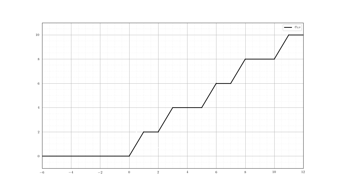
  Figure 2: MILP value function $\phi_{IP}$ (24)

  ∎∎

The function shown in Figure 2 is observed to be piecewise linear, non-decreasing, non-convex, and non-concave. These are all properties of general value functions of the form (22), but there are also several other important properties that are not evident from this simple example. In particular, the value function may be discontinuous, but is always lower semi-continuous and also subadditive.

Another important property of $\phi_{IP}$ that is evident from Figure 2 is that its epigraph is the union of a set of convex radial cones. These cones are translations of the epigraph of the value function of a single parametric LP, the so-called continuous restriction of the given MILP (defined later in Section 4.2) resulting from fixing the integer variables. Hassanzadeh and Ralphs [2014b] further proved that the value function can be described within any bounded region by specifying a finite set of points of strict local convexity of $\phi_{IP}$, which are the locations of the extreme points of these radial cones (assuming the epigraph of the LP value function is a pointed cone). This resulted in a finite discrete representation of $\phi_{IP}$ (see Hassanzadeh and Ralphs [2014b] for additional details and formal results).

Although there exist effective algorithms for evaluating $\phi_{IP}$ for a single fixed right-hand side $\hat{\beta}$ (e.g., any method for solving the associated MILP), it is difficult to explicitly construct the entire function because this evidently requires solution of a sequence of MILPs. Algorithms for evaluating $\phi_{IP}$ at a right-hand side $\hat{\beta}$, such as branch-and-bound algorithm, do, however, produce information about its structure beyond the single value $\phi_{IP}(\hat{\beta})$. This information comes in the form of a dual function that is strong at $\hat{\beta}$. We next describe the form and structure of these dual functions.

Dual Functions.

We focus here on dual functions from the branch-and-bound algorithm, which is the most widely used solution method for solving MILPs. We refer the reader to Güzelsoy [2009] and Güzelsoy and Ralphs [2007] for an overview of other methods. Wolsey [1981] was the first to propose that dual functions could be extracted from branch-and-bound trees, as described in the following result.

Theorem 2 (Wolsey [1981], Theorem 19).

Let $\hat{\beta}\in\mathbb{R}^{m_{2}}$ be such that $\phi_{IP}(\hat{\beta})<\infty$ and suppose $T$ is the set of indices of leaf nodes of a branch-and-bound tree resulting from evaluation of $\phi_{IP}(\hat{\beta})$. Then there exists a dual function $\underline{\phi}_{IP}:\mathbb{R}^{m_{2}}\rightarrow\mathbb{R}\cup\{\pm\infty\}$ of the form

$$\underline{\phi}_{IP}(\beta)=\min_{t\in T}\ \left(\beta^{\top}\eta^{t}+\alpha^{t}\right)\quad\forall\beta\in\mathbb{R}^{m_{2}},$$ (25)

where $\eta^{t}\in\mathbb{R}^{m_{2}}$ is an optimal solution to the dual of the LP relaxation associated with node $t$ and $\alpha^{t}\in\mathbb{R}$ is the product of the optimal reduced costs and variable bounds of this LP relaxation. Further, $\underline{\phi}_{IP}$ is strong at $\hat{\beta}$, i.e., $\underline{\phi}_{IP}(\hat{\beta})=\phi_{IP}(\hat{\beta})$.

The interpretation of the function $\underline{\phi}_{IP}$ in (25) is conceptually straightforward. The solution to the LP relaxation of node $t$ of the branch-and-bound tree yields the dual function $\beta^{\top}\eta^{t}+\alpha^{t}$, which bounds the optimal value of the relaxation problem associated with that node. The overall lower bound yielded by the tree is then the smallest bound yielded by any of the leaf nodes. This is the usual lower bound yielded by a branch-and-bound-based MILP solver during the solution process. Finally, we obtain $\underline{\phi}_{IP}$ by interpreting the optimal solution to the dual of the LP relaxation in each node as a function of $\beta$. There are additional subtle details involving construction of appropriate dual functions for infeasible nodes, but we omit these details here.

In principle, stronger dual functions can be obtained. For example, stronger functions can be constructed from the branch-and-bound tree by considering non-leaf nodes, suboptimal dual solutions arising during the solution process, full LP value function at each leaf node $t$ instead of a single hyperplane $\beta^{\top}\eta^{t}+\alpha^{t}$, etc. Further details on these methods are mentioned in Güzelsoy and Ralphs [2007] and Hassanzadeh and Ralphs [2014a].

• Figure 3 shows the dual functions obtained upon applying the result in Theorem 2 to the MILP (24). We solve this MILP with three values of the right-hand side $\beta$.

  

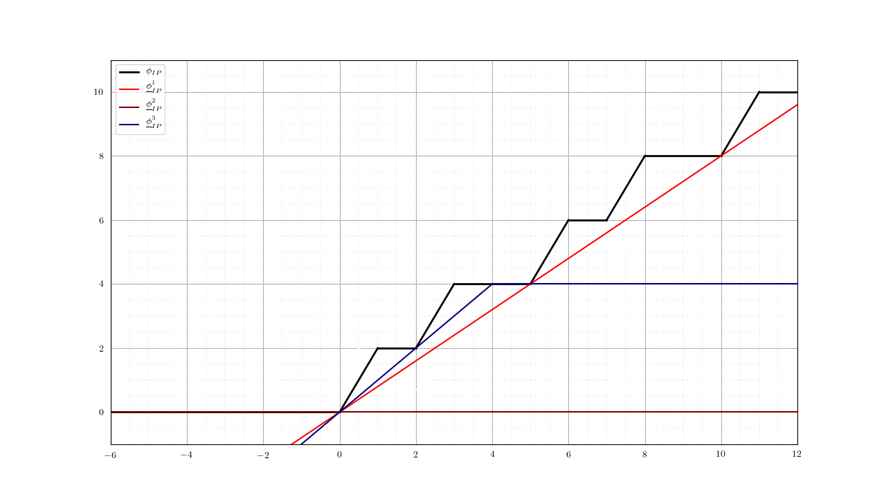
  Figure 3: Dual functions for (24)

  • $\beta=5$: There is only one node in the associated branch-and-bound tree with the optimal dual solution $\eta=0.8$, $\underline{\eta}=(0.4,0,1.4,2.4)$, and $\overline{\eta}=(0,0,0,0)$. This results in the dual function

    $$\underline{\phi}_{IP}^{1}(\beta)=0.8\beta\quad\forall\beta\in\mathbb{R}.$$

  • $\beta=0$: There is still only one node in the tree with the optimal dual solution $\eta=0$, $\underline{\eta}=(2,4,3,4)$, and $\overline{\eta}=(0,0,0,0)$. This results in the dual function

    $$\underline{\phi}_{IP}^{2}(\beta)=0\quad\forall\beta\in\mathbb{R}.$$

  • $\beta=2$: There are three nodes in the tree, i.e., one root node and two leaf nodes resulting from the branching disjunction $y_{2}\leq 0\vee y_{2}\geq 1$. The optimal dual solution and the resulting dual function $\beta^{\top}\eta^{t}+\alpha^{t}$ at each leaf node $t$ are mentioned in Table 1.

    Table 1: Data for construction of the dual function from the branch-and-bound tree in Example 3.2.1

    $t$	Branching constraint	$\eta^{t}$	$\underline{\eta}^{t}$	$\overline{\eta}^{t}$	$\beta^{\top}\eta^{t}+\alpha^{t}$
    1	$y_{2}\leq 0$	1	(0, 0, 1, 2)	(0, -1, 0, 0)	$\beta$
    2	$y_{2}\geq 1$	0	(2, 4, 3, 4)	(0, 0, 0, 0)	4

    This results in the dual function

    $$\underline{\phi}_{IP}^{3}(\beta)=\min\{\beta,4\}\quad\forall\beta\in\mathbb{R}.$$

  Naturally, as in the formulation of the master problem, the value function approximation can be improved by taking the maximum of multiple dual functions strong at different right-hand sides. In the above example, the dual function $\max\{\underline{\phi}_{IP}^{1}(\beta),\underline{\phi}_{IP}^{2}(\beta),\underline{\phi}_{IP}^{3}(\beta)\}$ is already seen to be a reasonable approximation of the full value function. ∎∎

As mentioned earlier, solving the subproblem in an iteration requires evaluating $\phi_{IP}$ at $|\Omega|$ right-hand side vectors corresponding to $|\Omega|$ scenarios, for a fixed first-stage solution. Specifically, in iteration $k$ of the algorithm, we solve

$$\phi_{IP}(b^{2}_{\omega}-A^{2}_{\omega}x^{k})=\min \;{d^{2}}^{\top}y$$

s.t. $$\;G^{2}y\geq b^{2}_{\omega}-A^{2}_{\omega}x^{k}$$

$$\quad y\in Y$$

for all $\omega\in\Omega$, where $x^{k}$ is the fixed first-stage solution in the current iteration. The result is a scenario dual function ${\underline{\phi}_{IP}^{k}}_{\omega}$ of the form (25) for each $\omega\in\Omega$.

3.2.2 Master Problem

By exploiting the specific structure of the dual functions described in the previous section, we can straightforwardly adapt the algorithmic framework from Section 2 to obtain an algorithm for solving (21) similar to that derived by the authors in Hassanzadeh and Ralphs [2014a].

Introducing auxiliary variables $z_{\omega}$ for each scenario, as in previous reformulations, we obtain the master problem in iteration $k$ as

$$\min \;c^{\top}x+\sum_{\omega\in\Omega}p_{\omega}z_{\omega}$$ (26)

s.t. $$\ A^{1}x\geq b^{1}\;$$

$$\;z_{\omega}\geq\max_{1\leq i\leq k}{\underline{\phi}_{IP}^{i}}_{\omega}(b^{2}_{\omega}-A^{2}_{\omega}x)\quad\forall\omega\in\Omega$$

$$\ x\in X.$$

Because each scenario dual function is the minimum of a collection of affine functions, the overall master problem can be eventually reformulated as an MILP by introducing additional binary variables (see Hassanzadeh and Ralphs [2014a] for details).

3.2.3 Overall Algorithm

Putting this all together, in each iteration $k$, a master problem of the form (26) is solved to obtain its optimal solution $(x^{k},\{z^{k}_{\omega}\}_{\omega\in\Omega})$ and a lower bound. Following that, the subproblem is solved, which consists of evaluating $\phi_{IP}(b^{2}_{\omega}-A^{2}_{\omega}x^{k})$ for each $\omega\in\Omega$ using a branch-and-bound algorithm. The result is a strong dual function (25) for each scenario, as well as an overall upper bound. If the upper and lower bounds are equal, then we are done. Otherwise, the dual functions are fed back into the master problem and the method is iterated until the upper and lower bounds converge.

4 Mixed Integer Bilevel Linear Optimization Problems

We now move on to a detailed discussion of the application of this generalization of Benders’ principle to MIBLPs. As described earlier, MIBLPs are two-stage MMILPs in which the variables at each stage are conceptually controlled by different DMs with different objective functions. MIBLPs model problems in game theory, specifically the Stackelberg games introduced by Von Stackelberg [1934]. Bilevel optimization problems in the form presented here were formally introduced and the term was coined in the 1970s by Bracken and McGill [1973], but computational aspects of such optimization problems have been studied since at least the 1960s (see, e.g., Wollmer [1964]). Most of the initial research was limited to continuous bilevel linear optimization problems containing only continuous variables and linear constraints in both the stages.

Study of bilevel optimization problems containing integer variables and algorithms for solving them is generally acknowledged to have been initiated by Moore and Bard [1990], who discussed the computational challenges of solving such problems and suggested one of the earliest algorithms, a branch-and-bound algorithm, which converges to an optimal solution if all first-stage variables are integer or all second-stage variables are continuous. Since then, many works have focused on special cases, such as those in which the first-stage variables are all binary or all second-stage variables are continuous. It is only in the past decade or so that study of exact algorithms for the general case in which there are both continuous and general integer variables in both stages has been undertaken.

Table 2 provides a timeline of the main developments in the evolution of such exact algorithms, indicating the types of variables supported in both the first and second stages (C indicates continuous, B indicates binary, and G indicates general integer). Most of these works are either pure cutting plane or branch-and-cut algorithms in the full space of first- and second-stage variables, and hence, are not technically included under the umbrella of the framework of this paper. Only three works, Saharidis and Ierapetritou [2009], Zeng and An [2014] and Yue et al. [2019], present themselves as decomposition algorithms. Of these three, only the first work is a pure Benders-type algorithm, but it focuses on the special case with all continuous second-stage variables, in which case the reformulation can be done using standard KKT conditions and the Benders’ cuts are linear. The other two works deviate from our approach in significant ways since their master problems are in the full space of first- and second-stage variables.

Although no existing algorithm for the general MIBLP case can be considered as a pure Benders-type algorithm, there nevertheless must necessarily be some connection between all algorithms for solving MIBLPs because of the necessity to at least implicitly construct primal approximations of the MILP value function (22), a topic introduced in Section 4.2. In the particular case when the objective functions for the two stages disagree, such primal approximation of the value function cannot be avoided. But while this need for primal approximation may make it appear as if some algorithmic alternatives are also in fact Benders-type algorithms, it is the need for explicit dual approximations that sets such algorithms apart. The dual approximation is necessary precisely because of the projection operation that is necessary when the second-stage variables are not present in the master problem. Once second-stage variables are present in the master problem, the dual approximation is no longer needed. With respect to the specific algorithmic step of constructing primal functions, the construction methods of existing works can be seen as special cases of our method, which is to construct a parametric primal function (34) (see Section 4.2). For example, the primal functions in Lozano and Smith [2017] and Yue et al. [2019] are (non-parametric) constant functions, and those in Caprara et al. [2016] are a special case that exploits the specific structure of the problem to obtain parametric functions that are linear in the first-stage variables.

Table 2: Evolution of algorithms for bilevel optimization

Citation	Stage 1 Variable Types	Stage 2 Variable Types
Wen and Yang [1990]	B	C
Bard and Moore [1992]	B	B
Faísca et al. [2007]	B, C	B, C
Garcés et al. [2009]	B	C
Saharidis and Ierapetritou [2009]	B, C	C
DeNegre and Ralphs [2009], DeNegre [2011]	G	G
Köppe et al. [2010]	G or C	G
Baringo and Conejo [2012]	B, C	C
Xu and Wang [2014]	G	G, C
Zeng and An [2014]	G, C	G, C
Caramia and Mari [2015]	G	G
Caprara et al. [2016]	B	B
Hemmati and Smith [2016]	B, C	B, C
Lozano and Smith [2017]	G	G, C
Wang and Xu [2017]	G	G
Fischetti et al. [2017], Fischetti et al. [2018]	G, C	G, C
Yue et al. [2019]	G, C	G, C
Tahernejad et al. [2020]	G, C	G, C

4.1 Formulation

To state the class of problems formally, we must introduce a type of constraint that cannot be expressed in the canonical language of mathematical optimization. In addition to the usual linear constraints, we have a constraint that requires the second-stage solution to be optimal with respect to a problem that is parametric in the first-stage solution. The formulation including this constraint, as it usually appears in the literature on bilevel optimization, is

$$\min \;c^{\top}x+{d^{1}}^{\top}y$$ (27)

s.t. $$\text{ }A^{1}x+G^{1}y\geq b^{1}$$

$$\;x\in X$$

$$y\in\arg\min\;\{{d^{2}}^{\top}\check{y}$$

$$\quad\text{s.t.}\;G^{2}\check{y}\geq b^{2}-A^{2}x$$

$$\quad\check{y}\in Y\},$$

where $A^{1}\in\mathbb{Q}^{m_{1}\times n_{1}}$, $G^{1}\in\mathbb{Q}^{m_{1}\times n_{2}}$, $b^{1}\in\mathbb{Q}^{m_{1}}$, $A^{2}\in\mathbb{Q}^{m_{2}\times n_{1}}$, $G^{2}\in\mathbb{Q}^{m_{2}\times n_{2}}$, $b^{2}\in\mathbb{Q}^{m_{2}}$, $c\in\mathbb{Q}^{n_{1}}$, $d^{1}\in\mathbb{Q}^{n_{2}}$, and $d^{2}\in\mathbb{Q}^{n_{2}}$. Note that the above-mentioned parametric problem is nothing but the evaluation of $\phi_{IP}(b^{2}-A^{2}x)$, where $\phi_{IP}$ is the MILP value function (22).

Underlying the above formulation are a number of assumptions. First, there is an implicit assumption that whenever the evaluation of $\phi_{IP}(b^{2}-A^{2}x)$ yields multiple optimal solutions, the one that is most advantageous for the first-stage DM is chosen. This form of MIBLP is known as the optimistic case and is just one of several variants. The pessimistic variant, for example, is one in which the second-stage solution chosen is always the one least advantageous for the first-stage DM. It should also be pointed out that we explicitly allow the second-stage variables in the constraints $A^{1}x+G^{1}y\geq b^{1}$. This is rather non-intuitive but there are applications for which this is a necessary element. We now define so-called linking variables.

Definition 4 (Linking Variables).

Linking variables are the first-stage variables whose indices are in the set

$$L=\left\{i\in\{1,\ldots,n_{1}\}\mid A^{2}_{i}\neq 0\right\},$$

where $A^{2}_{i}$ denotes the $i^{\textrm{th}}$ column of $A^{2}$.

Assumption 1.

All linking variables are integer variables.

This assumption is required to ensure the existence of an optimal solution for the given MIBLP. The optimal solution may not be attainable when there are linking variables that are continuous and second-stage variables that are integer [Moore and Bard, 1990, Vicente et al., 1996, Köppe et al., 2010].

Assumption 2.

All first-stage variables are linking variables.

Since we focus on optimistic bilevel problems, all non-linking variables can simply be moved to the second stage without loss of generality. This assumption is made primarily for ease of exposition, nevertheless results in a mathematically equivalent MIBLP, despite the inconsistency with the intent of the original model. In combination with Assumption 1, this assumption implies that all first-stage variables are integer variables, i.e., $n_{1}=r_{1}$.

Assumption 3.

The set

$$\{(x,y)\in\mathbb{R}^{n_{1}}_{+}\times\mathbb{R}^{n_{2}}_{+}\mid y\in{\cal P}_{1}(b^{1}-A^{1}x)\cap{\cal P}_{2}(b^{2}-A^{2}x)\}$$

is bounded, where

$${\cal P}_{1}(\beta^{1})=\left\{y\in\mathbb{R}_{+}^{n_{2}}\;\middle|\;G^{1}y\geq\beta^{1}\right\}$$

and ${\cal P}_{2}(\beta^{2})$ (as defined in (23)) represent families of polyhedra consisting of all points satisfying $G^{1}y\geq\beta^{1}$ and $G^{2}y\geq\beta^{2}$ for given right-hand sides $\beta^{1}\in\mathbb{R}^{m_{1}}$ and $\beta^{2}\in\mathbb{R}^{m_{2}}$. Assumption 3 is made to avoid uninteresting cases involving unboundedness, but is easy to relax in practice.

Assumption 4.

For all $x\in\mathbb{R}^{n_{1}}$, we have

$$\phi_{IP}(b^{2}-A^{2}x)>-\infty,$$

or, equivalently

$$\left\{r\in\mathbb{R}^{n_{2}}_{+}\;\middle|\;G^{2}r\geq 0,{d^{2}}^{\top}r<0\right\}=\emptyset.$$

Assumption 4 is also made to avoid uninteresting cases involving unboundedness. Observe that in the case $\phi_{IP}(b^{2}-A^{2}x)=-\infty$ for a given value of $x$, then $\phi_{IP}(b^{2}-A^{2}x)=-\infty$ for all values of $x$. Note that Assumptions 2-4 can be relaxed in practice.

4.2 Projection

We now apply the familiar operations of Benders’ framework to the formulation (27). Upon projecting into the space of the first-stage variables, we obtain the reformulation

$$\min_{x\in X}\left\{c^{\top}x+\rho(b^{1}-A^{1}x,\;b^{2}-A^{2}x)\right\},$$ (28)

where $\rho$ is the second-stage reaction function, defined as

$$\rho(\beta^{1},\beta^{2})=\min\left\{{d^{1}}^{\top}y\;\middle|\;y\in{\cal P}_{1}(\beta^{1}),\;y\in\arg\min\left\{{d^{2}}^{\top}\check{y}\;\middle|\;\check{y}\in{\cal P}_{2}(\beta^{2})\cap Y\right\}\right\}.$$ (29)

Observe that the reaction function has embedded within it exactly the kind of optimality constraint we tried to eliminate by using projection to reformulate the given MIBLP. Although the reaction function appears at first to be the value function of a general bilevel optimization problem, it is actually the value function of a lexicographic MILP. To see this, note that the evaluation of $\rho(\beta^{1},\beta^{2})$ for known values of $(\beta^{1},\beta^{2})$ can be done in two steps. First, we evaluate MILP

$$\phi_{IP}(\beta^{2})=\min\left\{{d^{2}}^{\top}\check{y}\;\middle|\;\check{y}\in{\cal P}_{2}(\beta^{2})\cap Y\right\}.$$

Then, we have

$$\rho(\beta^{1},\beta^{2})=\min\left\{{d^{1}}^{\top}y\;\middle|\;{d^{2}}^{\top}y\leq\phi_{IP}(\beta^{2}),y\in{\cal P}_{1}(\beta^{1})\cap{\cal P}_{2}(\beta^{2})\cap Y\right\},$$ (30)

which is an MILP. In other words, the evaluation of $\rho(\beta^{1},\beta^{2})$ is an optimization problem over the set of optimal solutions to a given (non-parametric) MILP. Once $\phi_{IP}(\beta^{2})$ is known, the set of optimal solutions over which we are trying to optimize is the feasible set of an MILP. The reason this is not a bilevel optimization problem is simply because the right-hand side vector $\beta^{2}$ is not parametric, i.e., it is a known vector. In the next part of this section, we examine the properties and structure of the reaction function before discussing how to construct associated dual functions.

Reaction Function.

As with all value functions, $\rho(\beta^{1},\beta^{2})=\infty$ for a given $(\beta^{1},\beta^{2})\in\mathbb{R}^{m_{1}}\times\mathbb{R}^{m_{2}}$ if either $\{y\in\mathbb{R}_{+}^{n_{2}}\mid y\in{\cal P}_{1}(\beta^{1})\cap{\cal P}_{2}(\beta^{2})\cap Y\}=\emptyset$ or $\phi_{IP}(\beta^{2})=-\infty$ (which cannot happen under Assumption 4), and $\rho(\beta^{1},\beta^{2})=-\infty$ for all $(\beta^{1},\beta^{2})\in\mathbb{R}^{m_{1}}\times\mathbb{R}^{m_{2}}$ if the lexicographic MILP is itself unbounded, i.e., $\{r\in\mathbb{R}^{n_{2}}_{+}\mid G^{1}r\geq 0,G^{2}r\geq 0,{d^{1}}^{\top}r<0\}\neq\emptyset$ (which cannot happen under Assumption 3).

We now illustrate the structure of the reaction function with a simple example. Although its structure is combinatorially more complex than that of the MILP value function, it nevertheless also has a piecewise polyhedral structure. We do not provide formal results concerning the structure and properties of the reaction function here, but these can be derived by application of techniques similar to those used to derive the structure of the MILP value function.

• Consider the following reaction function arising from an MIBLP with $G^{1}=0$.

  $$\rho(\beta) = \min \;-y_{1}+y_{2}-5y_{3}+y_{4}$$ (31)

  s.t. $$(y_{1},y_{2},y_{3},y_{4})\in\arg\min\;\{2\check{y}_{1}+4\check{y}_{2}+3\check{y}_{3}+4\check{y}_{4}$$

  $$\qquad\qquad\qquad\qquad\text{s.t.}\;2\check{y}_{1}+5\check{y}_{2}+2\check{y}_{3}+2\check{y}_{4}\geq\beta$$

  $$\qquad\qquad\qquad\qquad\qquad\check{y}_{1},\check{y}_{2},\check{y}_{3}\in\mathbb{Z}_{+},\ \check{y}_{4}\in\mathbb{R}_{+}\}$$

  This function can be reformulated as

  $$\rho(\beta) = \min \;-y_{1}+y_{2}-5y_{3}+y_{4}$$

  s.t. $$2y_{1}+5y_{2}+2y_{3}+2y_{4}\geq\beta$$

  $$2y_{1}+4y_{2}+3y_{3}+4y_{4}\leq\phi_{IP}(\beta)$$

  $$y_{1},y_{2},y_{3}\in\mathbb{Z}_{+},\ y_{4}\in\mathbb{R}_{+}.$$

  using the MILP value function $\phi_{IP}$, which is the same as for (24). The function $\rho$ is plotted in Figure 4.

  

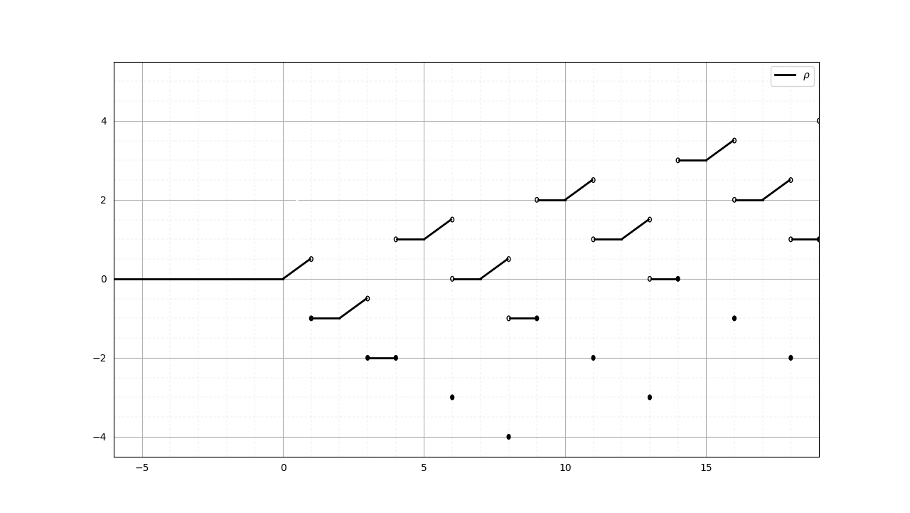
  Figure 4: Reaction function $\rho$ (31)

  ∎∎

As usual, we do not have an exact description of $\rho$ in general, so we cannot solve (28) directly, but instead replace $\rho$ in (28) with a dual function $\underline{\rho}$. Following the earlier procedure, this dual function is taken to be the maximum of the strong dual functions $\underline{\rho}^{k}$ obtained by solving a subproblem in each iteration $k$. The resulting master problem in iteration $k$ is

$$\min \;c^{\top}x+z$$ (32)

s.t. $$\;z\geq\underline{\rho}^{i}(b^{1}-A^{1}x,\;b^{2}-A^{2}x),\quad 1\leq i\leq k$$

$$x\in X.$$

Similarly, the subproblem in iteration $k$ is to evaluate $\rho(b^{1}-A^{1}x^{k},\;b^{2}-A^{2}x^{k})$ for the solution $x^{k}$ to (32), in order to construct a dual function $\underline{\rho}^{k}$ that is strong at $(b^{1}-A^{1}x^{k},\;b^{2}-A^{2}x^{k})$. We next detail the construction of this strong dual function.

Dual Functions.

As we have already noted, the subproblem in iteration $k$ is to evaluate the reaction function (29) for $(\beta^{1},\beta^{2})=(b^{1}-A^{1}x^{k},b^{2}-A^{2}x^{k})$. This problem is an MILP and we have the following theorem based on Theorem 2.

Theorem 3.

Let $(\hat{\beta^{1}},\hat{\beta}^{2})\in\mathbb{R}^{m_{1}}\times\mathbb{R}^{m_{2}}$ be such that $\rho(\hat{\beta^{1}},\hat{\beta}^{2})<\infty$ and suppose $T$ is the set of indices of leaf nodes of a branch-and-bound tree resulting from evaluation of $\rho(\hat{\beta^{1}},\hat{\beta}^{2})$. Then there exists a dual function $\underaccent{\tilde}{\rho}:\mathbb{R}^{m_{1}}\times\mathbb{R}^{m_{2}}\rightarrow\mathbb{R}\cup\{\pm\infty\}$ of the form

$$\underaccent{\tilde}{\rho}(\beta^{1},\beta^{2})=\min_{t\in T}\left({\beta^{1}}^{\top}\eta^{1,t}+{\beta^{2}}^{\top}\eta^{2,t}+\phi_{IP}(\beta^{2})\eta^{\phi,t}+\alpha^{t}\right)\quad\forall(\beta^{1},\beta^{2})\in\mathbb{R}^{m_{1}}\times\mathbb{R}^{m_{2}},$$ (33)

where $(\eta^{1,t},\eta^{2,t},\eta^{\phi,t})\in\mathbb{R}^{m_{1}}\times\mathbb{R}^{m_{2}}\times\mathbb{R}$ is a dual feasible solution of the LP relaxation associated with node $t$, and $\alpha^{t}\in\mathbb{R}$ is the product of reduced costs and variable bounds of this LP relaxation. Further, this dual function is strong at $(\hat{\beta}^{1},\hat{\beta}^{2})$ if $\underaccent{\tilde}{\rho}(\hat{\beta^{1}},\hat{\beta}^{2})=\rho(\hat{\beta^{1}},\hat{\beta}^{2})$.

The interpretation of this result is similar to the interpretation of Theorem 2. Let us look at an example that depicts these functions.

• Figure 5 shows five dual functions obtained upon applying the result in Theorem 3 to the reaction function (31) ($\underaccent{\tilde}{\rho}^{1}$ for $\beta=0$, $\underaccent{\tilde}{\rho}^{2}$ for $\beta=1$, $\underaccent{\tilde}{\rho}^{3}$ for $\beta=2$, $\underaccent{\tilde}{\rho}^{4}$ for $\beta=5$, and $\underaccent{\tilde}{\rho}^{5}$ for $\beta=8$).

  

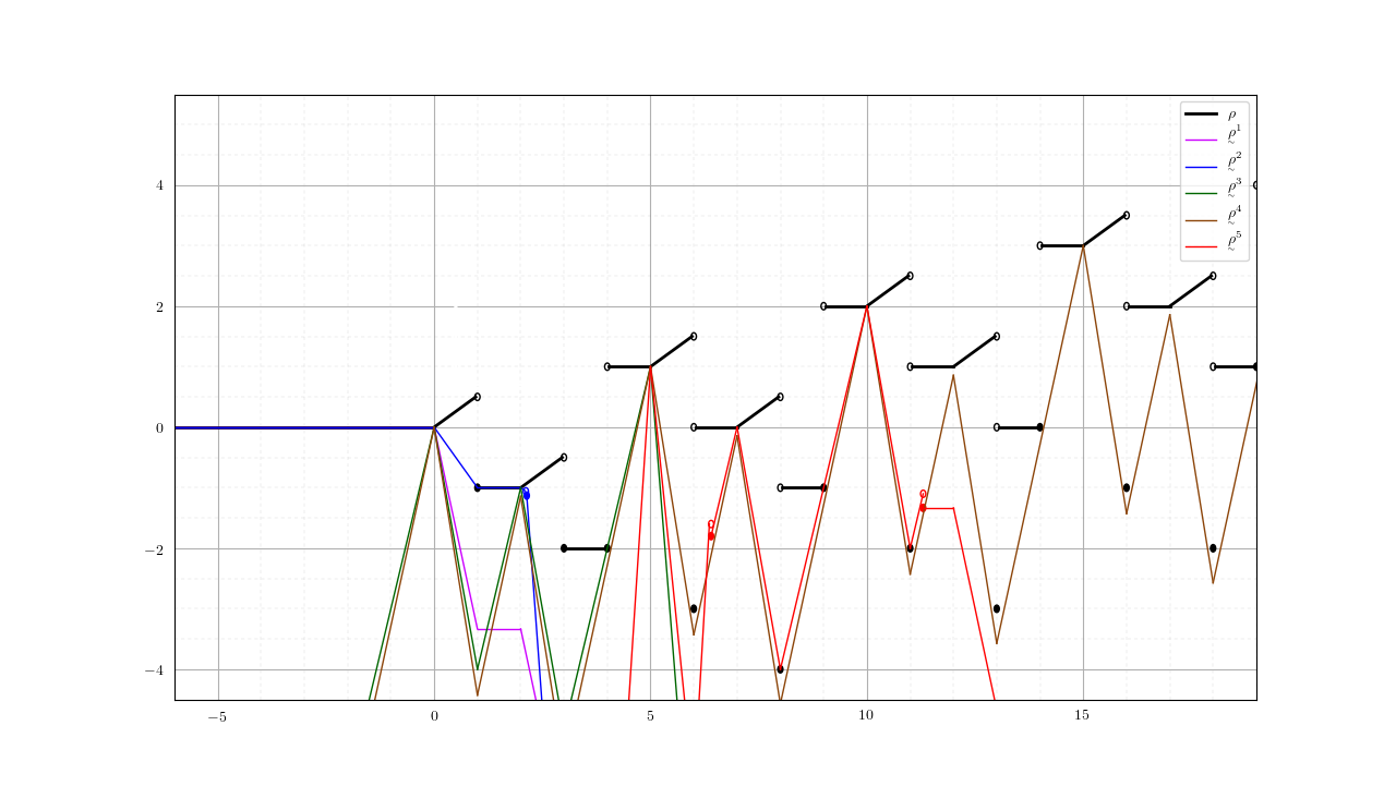
  Figure 5: Dual functions for (31)

  As expected, these dual functions are piecewise polyhedral. For example, solving (31) with $\beta=8$ as an equivalent MILP (after obtaining $\phi_{IP}(8)$ at first) yields the dual information (dual solution and reduced costs) from leaf nodes of the branch-and-bound tree shown in Table 3.

  Table 3: Data for construction of the dual function in Example 4.2

  $t$	Branching constraint	$(\eta^{2,t},\eta^{\phi,t})$	$\underline{\eta}^{t}$	$\overline{\eta}^{t}$	${\eta^{2,t}}^{\top}\beta+\eta^{\phi,t}\phi_{IP}(\beta)+\alpha^{t}$
  1	$y_{2}\geq 2$	$(0,-\frac{5}{3})$	$(\frac{7}{3},\frac{23}{3},0,\ \frac{7}{3})$	$(0,0,0,0)$	$-\frac{5}{3}\phi_{IP}(\beta)+\frac{46}{3}$
  2	$y_{2}\leq 1$, $y_{1}\leq 0$	$(11,-9)$	(0, 0, 0, 15)	(-5, -18, 0, 0)	$11\beta-9\phi_{IP}(\beta)-18$
  3	$y_{2}\leq 1$, $y_{1}\geq 1$, $y_{3}\leq 0$	$(3,-3.5)$	(0, 0, 0, 9)	(0, 0, -0.5, 0)	$3\beta-3.5\phi_{IP}(\beta)$
  4	$y_{2}\leq 1$, $y_{1}\geq 1$, $y_{3}\geq 1$	$(13,-16)$	(5, 0, 17, 39)	(0, 0, 0, 0)	$13\beta-16\phi_{IP}(\beta)+22$

This results in the dual function

$$\underaccent{\tilde}{\rho}^{5}(\beta)=\min\left\{-\frac{5}{3}\phi_{IP}(\beta)+\frac{46}{3},11\ \beta-9\phi_{IP}(\beta)-18,3\beta-3.5\phi_{IP}(\beta),13\beta-16\ \phi_{IP}(\beta)+22\right\},$$

containing the MILP value function $\phi_{IP}$. The remaining dual functions are obtained the same way. ∎∎

It is clear from Theorem 3 that the construction of $\underaccent{\tilde}{\rho}$ in (33) implicitly requires construction of the value function $\phi_{IP}$. However, the construction of $\phi_{IP}$ is itself a difficult task and generally impractical. Further, the complex structure of $\phi_{IP}$ makes the structure of $\underaccent{\tilde}{\rho}$ highly complex. To work around this difficulty, we replace $\phi_{IP}$ in (30) with a primal function, which bounds the value function from above and is strong at the given right-hand side. This replacement results in an alternative dual function (which we denote by $\underline{\rho}$) that is still strong at the given right-hand side. We use $\underline{\rho}$ in place of $\underaccent{\tilde}{\rho}$ in our work. To this end, we now embark on a small diversion into MILP primal functions.

Primal Functions.

In contrast with dual functions, strong primal functions bound the value function from above.

Definition 5 (Primal Function).

A primal function $P:\mathbb{R}^{m_{2}}\rightarrow\mathbb{R}\cup\{\pm\infty\}$ is one that satisfies $P(\beta)\geq\phi_{IP}(\beta)$ for all $\beta\in\mathbb{R}^{m_{2}}$. It is strong at $\hat{\beta}\in\mathbb{R}^{m_{2}}$ if $P(\hat{\beta})=\phi_{IP}(\hat{\beta})$.

An obvious way to construct such a function is to consider the value function of a restriction of the given MILP (see Güzelsoy [2009] and Güzelsoy and Ralphs [2007] for methods of construction). The following theorem presents the main result for constructing strong primal functions from restrictions of the given MILP.

Theorem 4 (Güzelsoy [2009], Theorem 3.39).

Consider the MILP value function (22). Let $K\subseteq N\coloneqq\{1,\ldots,n_{2}\},\;s\in\mathbb{R}^{|K|}_{+}$ be given, and define the function $\bar{\phi}_{N\setminus K}:\mathbb{R}^{m_{2}}{\rightarrow}\mathbb{R}\cup\{\pm\infty\}$ such that

$$\bar{\phi}_{N\setminus K}(\beta)=\sum_{i\in K}d^{2}_{i}s_{i}+\phi_{N{\setminus}K}\left(\beta-\sum_{i\in K}G^{2}_{i}s_{i}\right)\quad\forall\beta\in\mathbb{R}^{m_{2}},$$

where $G^{2}_{i}$ is the $i^{th}$ column of $G^{2}$ and

$$\phi_{N{\setminus}K}(\beta) = \min \;\sum_{i\in N{\setminus}K}d^{2}_{i}y_{i}$$

s.t. $$\;\sum_{i\in N{\setminus}K}G^{2}_{i}y_{i}\geq\beta$$

$$\ y_{i}\in\mathbb{Z}_{+}\text{ }\forall i\in I,\text{ }y_{i}\in\mathbb{R}_{+}\text{ }\forall i\in C,$$

where $I\subseteq N$ and $C\subseteq N$ represent sets of indices for integer and continuous variables respectively. Then, $\bar{\phi}_{N\setminus K}$ is a valid primal function of $\phi_{IP}$, i.e., $\bar{\phi}_{N\setminus K}(\beta)\geq\phi_{IP}(\beta)\text{ }\forall\beta\in\mathbb{R}^{m_{2}}$, if $s_{i}\in\mathbb{Z}_{+}\text{ }\forall i\in I\cap K$ and $s_{i}\in\mathbb{R}_{+}\text{ }\forall i\in C\cap K$. Further, the function $\bar{\phi}_{N\setminus K}$ will be strong at a given right-hand side $\hat{\beta}\in\mathbb{R}^{m_{2}}$ if and only if $s_{i}=y_{i}^{*}\;\forall i\in K$ where $y^{*}$ is an optimal solution of $\phi_{IP}(\hat{\beta})$.

By convention, for a known $\hat{\beta}\in\mathbb{R}^{m_{2}}$, we consider $\phi_{N{\setminus}K}(\hat{\beta})=\infty$ if the corresponding problem is infeasible and $\phi_{N{\setminus}K}(\hat{\beta})=-\infty$ if the problem is unbounded. The above result indicates that a primal function obtained from a restriction in which the values of certain variables have been fixed is strong at $\hat{\beta}\in\mathbb{R}^{m_{2}}$ if the fixed values of these variables correspond to those of an optimal solution at $\hat{\beta}$. A convenient approach is to fix all the integer variables to their optimal values. If there are no continuous variables in the problem, then the resulting primal function is

$$\bar{\phi}_{\emptyset}(\beta)=\left\{\begin{array}[]{ll}\sum\limits_{i\in I}d^{2}_{i}y_{i}^{*}&\text{if}\;\;\beta=\hat{\beta}\\ \infty&\text{otherwise}\end{array}\right.,$$

which is a single point, but still a valid strong primal function at $\hat{\beta}$. If continuous variables exist, then the restriction is a continuous restriction mentioned earlier. The resulting value function $\phi_{C}$ is nothing but the value function of an LP discussed briefly in Section 3.1. Let us now look at an example of using continuous restrictions to generate primal functions.

• Consider the MILP (24). Figure 6 demonstrates four primal functions obtained upon applying the result in Theorem 4 to this MILP. Specifically, $\bar{\phi}^{1}_{N\setminus K}$ for $\beta=0$, $\bar{\phi}^{2}_{N\setminus K}$ for $\beta=2$, $\bar{\phi}^{3}_{N\setminus K}$ for $\beta=4$, and $\bar{\phi}^{4}_{N\setminus K}$ for $\beta=5$. Here, we consider continuous restrictions of the given MILP. For example, for $\beta=0$, the optimal solution of (24) is $(0,0,0,0)$ resulting in the following continuous restriction.

  $$\phi_{C}(\beta)=\min\left\{4y_{4}\;\middle|\;2y_{4}\geq\beta,\;y_{4}\in\mathbb{R}_{+}\right\}\quad\forall\beta\in\mathbb{R}$$

  It is easy to observe that this LP value function is

  $$\phi_{C}(\beta)=\left\{\begin{array}[]{ll}0&\text{if}\;\;\beta\leq 0\\ 2\beta&\text{otherwise}\end{array}\right.,$$

  which itself is the required primal function $\bar{\phi}^{1}_{N\setminus K}$ because the integer component of the MILP objective function is zero. Other primal functions can be constructed in a similar way by solving the MILP with a new right-hand side, calculating the integer component of the MILP objective function at its optimal solution, and simply translating $\phi_{C}$ based on this integer component value.

  

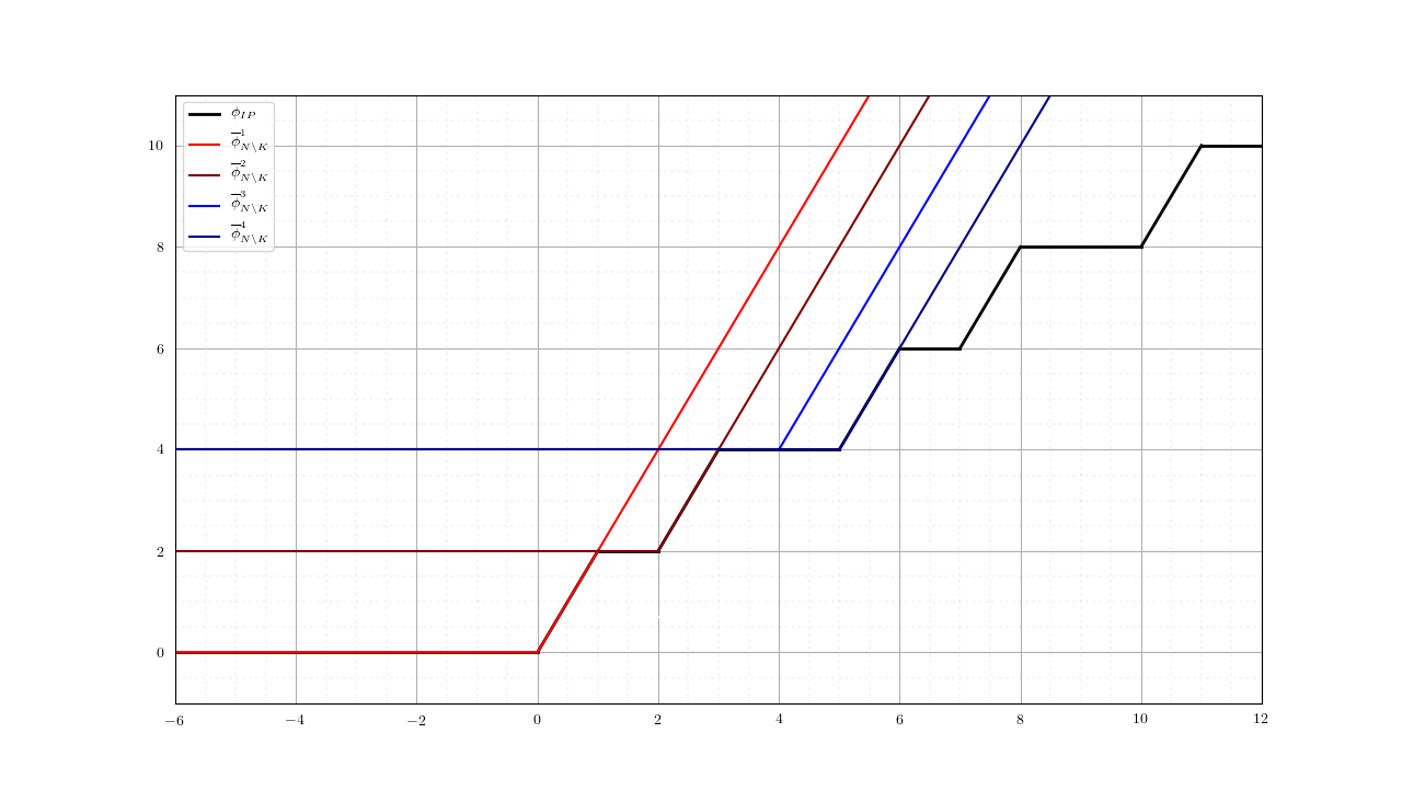
  Figure 6: Primal functions for (24)

  The primal function can be strengthened in the same way as dual functions are strengthened, by considering the minimum of multiple such (strong) functions. The epigraph of such a function is the minimum of convex radial cones and equals the epigraph of the value function when enough such cones are considered, as mentioned in Section 3.2.1. ∎∎

Although LPs are themselves easy to solve, obtaining a full description of the LP value function $\phi_{C}$ is still difficult, so we consider a partial function that we can easily obtain. Specifically, we use a single hyperplane of (16) to construct $\bar{\phi}_{N\setminus K}$. In Example 4.2, this is equivalent to considering only one of the two hyperplanes forming the cone corresponding to $\phi_{C}$. It is obvious from Figure 6 that any single hyperplane cannot form a valid primal function in the entire domain of the right-hand side vector. Therefore, we also need to restrict the domain of the right-hand side vector to only the region in which the single hyperplane is a valid upper bound.

Let $y^{*}=(y^{*}_{I},y^{*}_{C})$ be an optimal solution of an instance of (29) for a known right-hand side $(\hat{\beta}^{1},\hat{\beta}^{2})$, where $I$ and $C$ correspond to sets of indices of second-stage integer and continuous variables respectively. This inherently implies that $\phi_{IP}(\hat{\beta}^{2})={d^{2}}^{\top}y^{*}$. The value function $\phi_{C}$ of the continuous restriction is then

$$\phi_{C}(\beta)=\min \;{d^{2}_{C}}^{\top}y_{C}$$

s.t. $$\;G^{2}_{C}y_{C}\geq\beta$$

$$\ y_{C}\geq 0.$$

Let $\eta^{*}$ be an optimal solution of the dual of this LP, with right-hand side $\beta^{2}-G^{2}_{I}y^{*}_{I}$. Then ${\eta^{*}}^{\top}\beta$ is a dual function strong at $\beta^{2}-G^{2}_{I}y^{*}_{I}$. From the theory of LP duality, we know that this function provides a valid upper bound as long as $\eta^{*}$ remains optimal, which is the case for all $\beta$ such that $(G^{2}_{B})^{-1}\beta\geq 0$, where $B$ is the index set corresponding to the optimal basis and ${G^{2}_{B}}$ is the optimal basis matrix.

Thus, we obtain our final primal function with a restricted domain

$$\bar{\phi}_{IP}(\beta^{2})=\left\{\begin{array}[]{ll}\left(\beta^{2}-G^{2}_{I}y^{*}_{I}\right)^{\top}{\eta^{*}}+{d^{2}_{I}}^{\top}y^{*}_{I}&\text{if}\;{\left(G_{B}^{2}\right)}^{-1}\left(\beta^{2}-G^{2}_{I}y^{*}_{I}\right)\geq 0\\ \infty&\text{otherwise}\end{array}\right.$$ (34)

with which we replace $\phi_{IP}$ in (33). This ensures that the dual function $\underline{\rho}$ that we construct in each iteration of the algorithm is valid for all values of $(\beta^{1},\beta^{2})$.

4.3 Master Problem

Combining the results obtained in the previous section, the final form of $\underline{\rho}$ is

$$\underline{\rho}(\beta^{1},\beta^{2})=\min_{t\in T}\left({\beta^{1}}^{\top}\eta^{1,t}+{\beta^{2}}^{\top}\eta^{2,t}+\bar{\phi}_{IP}(\beta^{2})\eta^{\phi,t}+\alpha^{t}\right),$$ (35)

where $\bar{\phi}_{IP}$ is the primal function (34). This results in the optimality constraint

$$z\geq\min_{t\in T}\left({\beta^{1}}^{\top}\eta^{1,t}+{\beta^{2}}^{\top}\eta^{2,t}+\bar{\phi}_{IP}(\beta^{2})\eta^{\phi,t}+\alpha^{t}\right)$$ (36)

that we add to the master problem in each iteration of the algorithm, with $(\beta^{1},\beta^{2})=(b^{1}-A^{1}x,b^{2}-A^{2}x)$. Finally, the updated master problem after iteration $k$ of the algorithm is

$$\min \;c^{\top}x+z$$ (37)

s.t. $$\;z\geq\min_{t\in T_{i}}\left\{\left(b^{1}-A^{1}x\right)^{\top}\eta^{1,t}_{i}+\left(b^{2}-A^{2}x\right)^{\top}\eta^{2,t}_{i}+\bar{\phi}_{IP}^{i}(b^{2}-A^{2}x)\eta^{\phi,t}_{i}+{\alpha}^{t}_{i}\right\}\quad 1\leq i\leq k$$

$$\ x\in X,$$

where the vectors, matrices, sets, and functions with the subscript and superscript $i$ correspond to the information obtained in iteration $i\leq k$ of the algorithm.

4.4 Overall Algorithm

We now have all the components required for solving (27) with the generalized Benders’ decomposition algorithm in Figure 1. In each iteration $k$ of the algorithm, a master problem of the form (37) is solved to obtain its optimal solution $(x^{k},z^{k})$ and a global lower bound. Then, the subproblem is solved as an equivalent MILP, by evaluating (29) at $(b^{1}-A^{1}x^{k},b^{2}-A^{2}x^{k})$, to obtain a branch-and-bound tree and a global upper bound. Finally, an optimality constraint of the form (36) is constructed and added to the master problem to strengthen $z$. This constraint introduces some nonlinear components in the master problem but they can be linearized (as mentioned below) to obtain an MILP formulation for the master problem. These steps are repeated until the termination criterion is achieved.

We now illustrate the above discussion with an example.

• Consider the MIBLP

  $$\min x_{1}-3x_{2}-y_{1}+y_{2}-5y_{3}+y_{4}$$ (38)

  s.t. $$-x_{1}+2x_{2}\leq 1$$

  $$x_{1}\leq 3,\;x_{2}\leq 2,\;x_{1},x_{2}\in\mathbb{Z}_{+}$$

  $$(y_{1},y_{2},y_{3},y_{4})\in\arg\min\;\{2\check{y}_{1}+4\check{y}_{2}+3\check{y}_{3}+4\check{y}_{4}$$

  $$\qquad\qquad\qquad\qquad\text{s.t.}\;2\check{y}_{1}+5\check{y}_{2}+2\check{y}_{3}+2\check{y}_{4}\geq x_{1}+x_{2}$$

  $$\qquad\qquad\qquad\qquad\qquad\check{y}_{1},\check{y}_{2},\check{y}_{3},\in\mathbb{Z}_{+},\ \check{y}_{4}\in\mathbb{R}_{+}\},$$

  which is based on (24) and (31). Based on earlier discussion, we solve four optimization problems in iteration $k$ of the algorithm: a master problem, an MILP (24) (with $\beta^{k}=x^{k}_{1}+x^{k}_{2}$), a subproblem (31) (with $\beta^{k}=x^{k}_{1}+x^{k}_{2}$), and a continuous restriction of (24).

  Iteration 1. Our initial dual function is simply $\underline{\rho}^{0}(\beta)=-\infty$ for all $\beta\in\mathbb{R}^{m_{2}}$ and solving the initial master problem yields the optimal solution $(x_{1}^{1},x_{2}^{1})=(3,2)$ and $z^{1}=-\infty$, so that $\textrm{LB}^{1}=-\infty$. Then, we solve (24) with right-hand side $x_{1}^{1}+x_{2}^{1}=5$ to obtain $\phi_{IP}(x_{1}^{1}+x_{2}^{1})=4$. Next, we solve the subproblem to obtain its optimal solution $(y_{1}^{1},y_{2}^{1},y_{3}^{1},y_{4}^{1})=(0,1,0,0)$, so we have $\rho(x_{1}^{1}+x_{2}^{1})=1$ and $\textrm{UB}^{1}=x_{1}^{1}-3x_{2}^{1}+\rho(x_{1}^{1}+x_{2}^{1})=-2$. We obtain the dual information (dual solution, positive and negative reduced costs) shown in Table 4 from the branch-and-bound tree, which has only one node.

  Table 4: Data for construction of the dual function in Example 4.4.

  $t$	$(\eta_{1}^{2,t},\eta_{1}^{\phi,t})$	$(\underline{\eta}_{1}^{1,t},\ \underline{\eta}_{1}^{2,t},\underline{\eta}_{1}^{3,t},\underline{\eta}_{1}^{4,t})$	$(\bar{\eta}_{1}^{1,t},\bar{\eta}_{1}^{2,t},\bar{\eta}_{1}^{3,t},\bar{\eta}_{1}^{4,t})$	${\eta_{1}^{2,t}}^{\top}\beta+\eta_{1}^{\phi,t}\bar{\phi}_{IP}^{1}(\beta)+\alpha_{1}^{t}$
  1	(3.29, -3.86)	$(0.14,0,0,9.86)$	$(0,0,0,0)$	$3.29\beta-3.86\ \bar{\phi}_{IP}^{1}(\beta)$

Since $\textrm{UB}^{1}\not=\textrm{LB}^{1}$, we further solve the continuous restriction to obtain its optimal dual solution $\eta^{*}_{1}=0$ and optimal basis inverse matrix $(G^{2}_{B,1})^{-1}=[-1]$. Finally, we construct and add the dual function

$$\underline{\rho}^{1}(\beta)=\min\{3.29\beta-3.86\bar{\phi}_{IP}^{1}(\beta)\}=3.29\ \beta-3.86\bar{\phi}_{IP}^{1}(\beta),$$

where

$$\bar{\phi}_{IP}^{1}(\beta)=\left\{\begin{array}[]{ll}4&\text{if}\;\;\beta\leq 5\\ \infty&\text{otherwise.}\end{array}\right.,$$

to the master problem and proceed to the next iteration.

For conciseness, we now mention only $\underline{\rho}^{k}(\beta)$ and $\bar{\phi}_{IP}^{k}(\beta)$ obtained in each iteration $k$.

Iteration 2.

$$\underline{\rho}^{2}(\beta)=-\frac{5}{3}\bar{\phi}_{IP}^{2}(\beta)$$

$$\bar{\phi}_{IP}^{2}(\beta)=\left\{\begin{array}[]{ll}0&\text{if}\;\;\beta\leq 0\\ \infty&\text{otherwise}\end{array}\right.$$

Iteration 3.

$$\underline{\rho}^{3}(\beta)=\min\left\{0.5\bar{\phi}_{IP}^{3}(\beta),-4.5\ \bar{\phi}_{IP}^{3}(\beta)+8.5\right\}$$

$$\bar{\phi}_{IP}^{3}(\beta)=\left\{\begin{array}[]{ll}2&\text{if}\;\;\beta\leq 2\\ \infty&\text{otherwise}\end{array}\right.$$

Iteration 4.

$$\underline{\rho}^{4}(\beta)=\min\left\{-\dfrac{5}{3}\bar{\phi}_{IP}^{4}(\beta)+\ \dfrac{23}{3},17\beta-13\bar{\phi}_{IP}^{4}(\beta),\ -0.5\bar{\phi}_{IP}^{4}(\beta),\ 21\beta-26\bar{\phi}_{IP}^{4}(\beta)+40\right\}$$

$$\bar{\phi}_{IP}^{4}(\beta)=\left\{\begin{array}[]{ll}4&\text{if}\;\;\beta\leq 4\\ \infty&\text{otherwise}\end{array}\right.$$

Iteration 5. Solving the updated master problem yields $(x^{5}_{1},x^{5}_{2},z^{5})=(1,1,-1)$ and $\textrm{LB}^{5}=-3$. Solving the subproblem yields $(y_{1}^{5},y_{2}^{5},y_{3}^{5},y_{4}^{5})=(1,0,0,0)$, $\rho(x_{1}^{5}+x_{2}^{5})=-1$ and $\textrm{UB}^{5}=-3$. Since $\textrm{UB}^{5}=\textrm{LB}^{5}$, the termination criterion is achieved. Hence, we stop the algorithm with an optimal solution $(x_{1}^{*},x_{2}^{*},y_{1}^{*},y_{2}^{*},y_{3}^{*},y_{4}^{*})=(1,1,1,0,0,0)$.

Figure 7 shows the value function $\phi_{IP}$ and its primal functions obtained in every iteration. Similarly, Figure 8 shows the reaction function $\rho$ and its dual functions. The function values are infinite wherever there is no plot. These figures illustrate the fact that overall approximations of $\phi_{IP}$ and $\rho$ are strengthened after every iteration. After the final iteration, the approximation function values are the same as the exact function values at the right-hand side $x_{1}^{*}+x_{2}^{*}=2$.

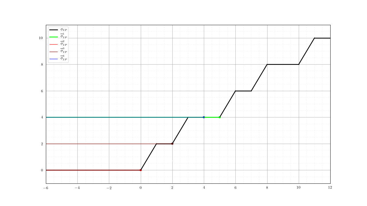
Figure 7: Primal functions constructed in the algorithm for solving (38)

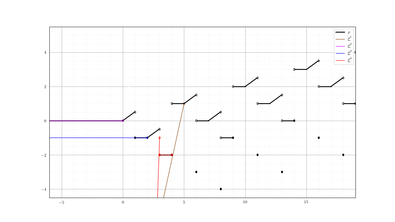
Figure 8: Dual functions constructed in the algorithm for solving (38)

∎∎

We now briefly discuss the linearization of the master problem (37). For notational simplicity, we drop the subscripts and superscripts denoting the algorithmic iteration. There are two types of nonlinearities in this problem: (1) the if-else condition in (34) and (2) the minimization operator in (35). We eliminate these nonlinearities by introducing binary variables and big-M parameters. This results in the following MILP form of the master problem.

$$\min \;c^{\top}x+z$$

s.t. $$\;z\geq\left(b^{1}-A^{1}x\right)^{\top}\eta^{1,t}+\left(b^{2}-A^{2}x\right)^{\top}\eta^{2,t}+\bar{\phi}_{IP}(b^{2}-A^{2}x)\eta^{\phi,t}+{\alpha}^{t}-M_{D}(1-u_{t})$$ (39a)

$$\sum\limits_{t\in T}u_{t}=1$$ (39b)

$$\ \bar{\phi}_{IP}(b^{2}-A^{2}x)=\left(b^{2}-A^{2}x-G^{2}_{I}y^{*}_{I}\right)^{\top}{\eta^{*}}+{d^{2}_{I}}^{\top}y^{*}_{I}+M_{P}v$$ (39c)

$$\ -\underline{M}v^{1}\leq{\left(G_{B}^{2}\right)}^{-1}\left(b^{2}-A^{2}x-G^{2}_{I}y^{*}_{I}\right)\leq\bar{M}\left(1-v^{1}\right)-\epsilon$$ (39d)

$$\ Mv-\sum\limits_{i\in\{1,\ldots,m_{2}\}}v^{1}_{i}\geq 0$$ (39e)

$$\ v-\sum\limits_{i\in\{1,\ldots,m_{2}\}}v^{1}_{i}\leq 0$$ (39f)

$$\ x\in X,z\text{ free},\bar{\phi}_{IP}\text{ free},u_{t}\in\mathbb{B}\;\forall t\in T,v\in\mathbb{B},v^{1}_{i}\in\mathbb{B}\;\forall i\in\{1,\ldots,m_{2}\}$$

Constraints (39a)-(39b) eliminate the minimization operator by adding the binary variables $u_{t}$ for $t\in T$ and the big-M parameter $M_{D}$. Constraints (39c)-(39f) eliminate the if-else condition by adding the binary variables $v$, $v_{i}^{1}$ for $i\in\{1,\ldots,m_{2}\}$ and the big-M parameters $\underline{M}$, $\bar{M}$ and $M$. Specifically, the constraints (39d)-(39f) impose domain restriction on the first-stage variables with respect to the primal function (34). This in turn restricts the domain of the right-hand sides for which $\phi_{IP}$ may be evaluated. The main idea is to set some $v^{1}_{i}=0$ whenever ${\left(G_{B_{i}}^{2}\right)}^{-1}\left(b^{2}-A^{2}x-G^{2}_{I}y^{*}_{I}\right)\geq 0$ and to set $v^{1}_{i}=1$ whenever ${\left(G_{B_{i}}^{2}\right)}^{-1}\left(b^{2}-A^{2}x-G^{2}_{I}y^{*}_{I}\right)<0$, where ${\left(G_{B_{i}}^{2}\right)}^{-1}$ is the $i^{\textrm{th}}$ row of the optimal basis matrix inverse. If at least one $v^{1}_{i}=1$, then $v=1$ further implying $\bar{\phi}_{IP}$ will have a very large value which is as required. If all $v^{1}_{i}=0$, then $v=0$ further implying $\bar{\phi}_{IP}$ will have a finite value which is also as required. Finally, $\epsilon$ is also a parameter corresponding to the domain restriction constraints added to deal with the strict inequality arising from “otherwise” condition in (34), and is the trickiest of all parameters to evaluate. The discussion on finding appropriate values of big-M and $\epsilon$ parameters is out of the scope of this paper.

5 Conclusions

We have described a generalization of Benders’ decomposition framework and illustrated its principles by applying it to several well-known classes of optimization problems that fall under the broad umbrella of MMILPs. The development of an abstract framework for generalizing the principles of Benders’ technique for reformulation that encompasses non-traditional problem classes, the specification of an associated algorithmic procedure, and its application to the class of MIBLPs are our main contributions. These stemmed from our observation that Benders’ framework can be viewed as a procedure for iterative refinement of dual functions associated with the value function arising from the projection of the original problem into the space of first-stage variables, and that this basic concept can be applied to a wide range of problems defined by additively separable functions.

A conceptual extension of the generalized Benders’ decomposition algorithm from MIBLPs to the case of general MMILPs is straightforward. Similar to MIBLPs, an $l$-stage MMILP can be formulated as a standard mathematical optimization problem by considering a constraint requiring values of all but first-stage variables to be optimal for an ($l-1$)-stage MMILP that is parametric in the first-stage variables, in addition to the usual linear constraints. Then, assuming that all input vectors and matrices are rational of appropriate dimensions without loss of generality, we have an $l$-stage MMILP with a parametric right-hand side $\beta$ defined as

$$\text{MMILP}^{l}(\beta)=\min \;{d^{11}}^{\top}x^{1}+{d^{12}}^{\top}x^{2}+\ldots+{d^{1l}}^{\top}x^{l}$$ (40)

s.t. $$\text{ }A^{11}x^{1}+A^{12}x^{2}+\ldots+A^{1l}x^{l}\geq\beta$$

$$\;x^{1}\in X^{1}$$

$$\ (x^{2},x^{3},\ldots,x^{l})\in\text{optimal set of $\text{MMILP}^{l-1}(b^{2}-A^{21}x^{1})$},$$

where $\text{MMILP}^{l-1}(b^{2}-A^{21}x^{1})$ denotes an ($l-1$)-stage MMILP with the parametric right-hand side $b^{2}-A^{21}x^{1}$, which in turn is a linear function of first-stage variables, defined similar to (40) but with $l-1$ variable vectors, as

$$\text{MMILP}^{l-1}(\beta)=\min \;{d^{22}}^{\top}x^{2}+{d^{23}}^{\top}x^{3}+\ldots+{d^{2l}}^{\top}x^{l}$$ (41)

s.t. $$\text{ }A^{22}x^{2}+A^{23}x^{3}+\ldots+A^{2l}x^{l}\geq\beta$$

$$\;x^{2}\in X^{2}$$

$$\ (x^{3},x^{4},\ldots,x^{l})\in\text{optimal set of $\text{MMILP}^{l-2}(b^{3}-A^{31}x^{1}-A^{32}x^{2})$}.$$

These formulations exhibit the natural recursive property of MMILPs that we spoke about in the beginning of the paper. It should be clear why this recursive structure also means that the proposed framework makes it easy to envision algorithms for solving such problems (whether these algorithms are practical is another question). We can project (40) (for a fixed $\beta=b^{1}$) into the space of the first-stage variables to obtain master and subproblems. The subproblem itself involves an ($l-1$)-stage MMILP (41), and solution of it calls for solving this ($l-1$)-stage MMILP. This ($l-1$)-stage MMILP can as well be solved with the generalized Benders’ principle due to the recursive structure. Strong dual functions can be constructed using techniques similar to those described earlier in the paper.

Although not discussed here, this framework can be readily applied to even broader classes of problems, such as those discussed in Bolusani et al. [2020], which incorporate stochasticity. While it is unclear whether such algorithms would be of practical interest, the algorithmic abstraction itself serves to illustrate basic theoretical principles, such as concepts of general duality and why $l$-stage MMILPs are canonical hard problems for stage $l$ of the polynomial time hierarchy.

The algorithms described in this paper are naive in the sense that their efficient implementations for practical purposes would require substantial additional development, especially for the classes of MIBLPs and MMILPs. To this end, our plans include enhancement of these algorithms by working in the areas of preprocessing techniques, warm starting of master and subproblem solves, cut management, a branch-and-Benders’-cut framework, alternative linearization techniques, and other enhancements, as well as incorporating aspects of these techniques into hybrid, non-Benders-type algorithms.

References

- Bachem and Schrader [1980] Bachem A, Schrader R (1980) Minimal equalities and subadditive duality. Siam Journal on Control and Optimization 18(4):437–443
- Balas [1979] Balas E (1979) Disjunctive programming. In: Annals of Discrete Mathematics 5: Discrete Optimization, North Holland, pp 3–51
- Bank et al. [1983] Bank B, Guddat J, Klatte D, Kummer B, Tammer K (1983) Non-linear Parametric Optimization. Birkhäuser verlag
- Bard and Moore [1992] Bard J, Moore J (1992) An algorithm for the discrete bilevel programming problem. Naval Research Logistics 39(3):419–435