A non-perturbative no-go theorem for photon condensation in approximate models

Abstract

Equilibrium phase transitions between a normal and a photon condensate state (also known as superradiant phase transitions) are a highly debated research topic, where proposals for their occurrence and no-go theorems have chased each other for the past four decades. Recent no-go theorems have demonstrated that gauge invariance forbids second-order phase transitions to a photon condensate state when the cavity-photon mode is assumed to be spatially uniform. However, it has been theoretically predicted that a collection of three-level systems coupled to light can display a first-order phase transition to a photon condensate state. Here, we demonstrate a general no-go theorem valid also for truncated, gauge-invariant models which forbids first-order as well as second-order superradiant phase transitions in the absence of a coupling with a magnetic field. In particular, we explicitly consider the cases of interacting electrons in a lattice and $M$-level systems.

I Introduction

The Dicke model dicke_pr_1954 is a paradigmatic model in the theory of light-matter interactions gross_pr_1982 ; cong_josaB_2016 ; kockum_naturereviewsphysics_2019 ; kirton19 . It describes a collection of ${N}$ identical two-level systems coherently coupled to the same bosonic mode $\hat{a}$, arising from the quantization of the electromagnetic field inside a cavity of volume $V$. As the name says, it was firstly introduced by Robert H. Dicke dicke_pr_1954 , with the aim of describing the “emission of coherent radiation” obtained by considering a “radiating gas as a single quantum-mechanical system”. He dubbed such process “super-radiant emission”.

In the thermodynamic limit (${N}\to\infty$, $V\to\infty$, with ${N}/V={\rm constant}$) and when the light-matter coupling strength exceeds a critical value, the Dicke model undergoes an equilibrium second-order thermal phase transition hepp_lieb ; wang_pra_1973 between a normal and a “super-radiant” phase. In the zero-temperature limit, the phase transition persists and corresponds to a quantum phase transition emary_brandes ; buzek_prl_2005 . The super-radiant phase is characterized by a macroscopic number of photons, $\langle\hat{a}\rangle\sim\sqrt{{N}}$, and by a macroscopic number of excitations in the matter sector. To avoid confusion with the Dicke non-equilibrium super-radiant emission dicke_pr_1954 , we here follow Refs. andolina_prb_2019 ; Andolina20 and dub the equilibrium super-radiant phase transition as “photon condensation”.

In the Coulomb gauge, a careful derivation of the Dicke model starting from a microscopic condensed-matter model with electronic degrees of freedom leads to an additional diamagnetic term rzazewski_prl_1975 , proportional to $(\hat{a}+\hat{a}^{\dagger})^{2}$, which is usually neglected by utilizing a (wrong) “weak-coupling argument”. It was soon understood rzazewski_prl_1975 ; Knight ; rzazewski_1979 that such additional term is crucial to preserve the gauge invariance property of the model. Only when both terms generated by the minimal coupling substitution $\hat{\bm{p}}\to\hat{\bm{p}}+e{\bm{A}}/c$, (i.e. the paramagnetic light-matter coupling and the diamagnetic term) are retained, does one have a gauge-invariant theory satisfying the Thomas-Reiche-Kuhn (TRK) sum rule Sakurai ; Tufarelli15 ; Savasta2021TRK . The occurrence of photon condensation in such a generalized Dicke model is forbidden rzazewski_prl_1975 ; rzazewski_prl_2006 ; nataf_naturecommun_2010 .

Despite its importance, the Dicke model is not exhaustive at all. In recent years, researchers have transcended it by studying interactions between matter degrees of freedom and quantized electromagnetic fields in a variety of other models and physical systems. Photon condensation has been predicted in many of these “beyond-Dicke” systems, including three-level systems Hayn11 ; Baksic13 , graphene hagenmuller_prl_2012 , ferroelectric materials keeling_jpcm_2007 , superconducting circuits nataf_naturecommun_2010 ; ciuti_prl_2012 ; Jaako16 ; Bamba16 , and strongly correlated (a.k.a. quantum) materials mazza_prl_2019 .

A number of no-go theorems for photon condensation in a single-mode spatially-uniform cavity field have appeared in the literature Gawedzki_pra_1981 ; Bamba_pra_2014 ; chirolli_prl_2012 ; pellegrino_prb_2014 ; viehmann_prl_2011 ; andolina_prb_2019 , showing that gauge invariance forbids photon condensation even in such “beyond-Dicke” systems. Often, theorems have been opposed by “go theorems” Vukics12 ; Stokes20 ; nataf_naturecommun_2010 . Photon condensation remains a rather controversial theoretical topic.

At present, the most recent no-go theorem is reported in Ref. andolina_prb_2019 , where the authors showed that photon condensation is forbidden by gauge invariance for generic non-relativistic interacting electron systems coupled to a spatially-uniform cavity mode. The proof is based on linear response theory Pines_and_Nozieres ; Giuliani_and_Vignale and uses the smallness of the order parameter $\alpha=\langle\hat{a}\rangle$. It is therefore valid only for second-order phase transitions, where $\alpha\ll 1$ at the phase transition, and changes continuously. It is by now clear that a natural path to overcome such theorem is to consider spatially-varying cavity fields guerci ; Basko19 ; Andolina20 . In these recent works, photon condensation has been shown to occur and is essentially a magneto-static instability Basko19 ; Andolina20 ; guerci ; Zueco20 . Apparently, another possibility to bypass the hypothesis of such theorem could be to consider a first-order phase transition Hayn11 ; Baksic13 , where the order parameter $\alpha$ abruptly changes from zero (in the normal phase) to a finite value (in the photon condensate phase). As a matter of fact, that first-order phase transitions were a valuable possibility to overcome the no-go theorem was first discussed some time ago ciuti_prl_2012 ; ReplyViehmann . In these works, an ensemble of three level systems coupled to single uniform mode undergoes to first-order phase transition. Indeed, according to Refs. ciuti_prl_2012 ; ReplyViehmann systems displaying first-order phase-transitions were thought as valuable candidates to realize photon condensation.

These results are, however, in contrast with a rather general no-go theorem presented already in 1978 Knight . In this work, an ensemble of electrons in the presence of single-particle potentials and interacting with a uniform electromagnetic mode is considered and it is shown that superradiant phase transitions (of any order) to a photon condensate are forbidden. In this proof, no truncation is taken and the full infinite-dimensional Hilbert space is retained. However, it is often impractical to deal with an exponentially large Hilbert space. Hence, when performing explicit calculations in atomic systems, or more generally, in many-body systems, approximate (truncated) models are customarily employed. However, it has been shown that such approximations can spoil gauge invariance DiStefano19 . Since no-go theorems are closely related to gauge-invariance, it is natural to conclude that the super-radiant phase transition that can be found in these approximate models (e.g. in the three-level systems discussed in Refs. Hayn11 ; Baksic13 ) is a fictitious effect due to the Hilbert space truncation. Since, in the ultra strong coupling, these models fails in describing the correct ground state, it is important to find a systematic procedure to construct truncated models fulfilling gauge-invariance and free of spurious phase transition. It has been shown that, even for these approximate models, it is possible to build light-matter interactions which consistently satisfy the gauge-invariance principle DiStefano19 ; Garziano20 ; Savasta21 . Here, we extend the no-go theorem for photon condensation of Ref. Knight for gauge-invariant truncated models of light-matter interacting systems. In particular, in the first part of this Article, we consider an interacting system of electrons roaming in free space and on a lattice and we extend the no-go theorem of Ref. Knight to such a system. In the second part of this Article, we present a no-go theorem for a generic $M$-level matter system interacting with a uniform electromagnetic field. On the basis of our new no-go theorem, we conclude that the first-order phase transition phenomenology discussed in the pioneering works Hayn11 ; Baksic13 on three-level systems coupled to a cavity mode is incorrect. The reason is that, in these models, the light-matter interaction was not derived from an underlying gauge-invariant model. Conversely, an ad hoc diamagnetic term was added. Such addition, which was made to enforce the TRK sum-rule Sakurai ; Tufarelli15 ; Savasta2021TRK , is not always sufficient to prevent a breakdown of gauge invariance. While enforcing the TRK sum-rule alone was a reasonable approach at the time that Refs. Hayn11 ; Baksic13 were published, nowadays more refined techniques to enforce gauge invariance in systems with an arbitrary but finite number of levels have been developed DiStefano19 ; Garziano20 ; Savasta21 ; Roman22 and applied to a few solid-state systems Schiro20 ; Li20b ; Li22 . Such methods can be viewed as an application of lattice gauge theory Wiese . Here, we also employ these new tools to derive a fully gauge-invariant model describing $M$-level systems coupled to a cavity mode. In accordance with the general theorem, such model does not display photon condensation. As an example, we analyze in detail an ensemble of three-level systems.

Our Article is organized as following. In Sect. II we present a non-perturbative no-go theorem for photon condensation in the second-quantization framework. We consider both the continuum case and the case of Hilbert-space truncation on a lattice. In Sect. III we present a non-perturbative no-go theorem for photon condensation, valid for a generic $M$-level matter system interacting with the electromagnetic field via the electric dipole moments. Finally, in Sect. IV we draw our main conclusions.

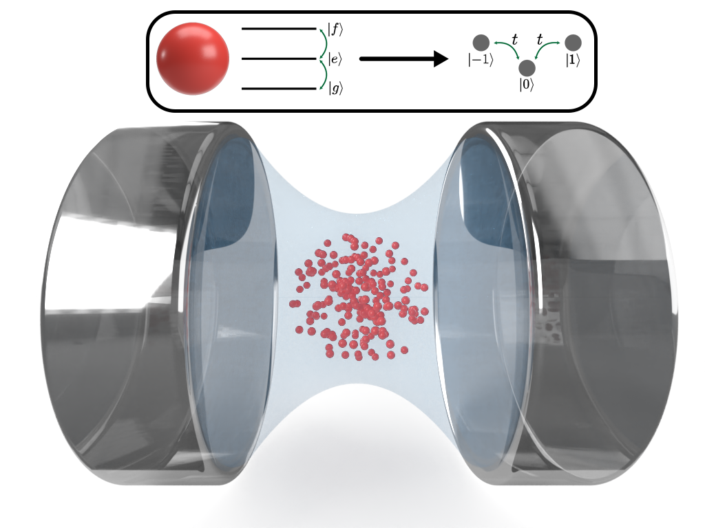
Figure 1: Pictorial representation of an ensemble of three-level atoms interacting with a cavity field. Each atom, which is considered in a ladder configuration, can be seen as a three-sites system with nearest neighbor hopping and parity symmetry. According to the lattice gauge theory, the interaction with the electromagnetic field can be obtained using the Wilson parallel transporter.

II Gauge invariance, photon condensation, and no-go theorem in interacting electron systems

II.1 Interacting electron system in the continuum

We consider a quantum many-body system of interacting electrons, following the notation of Ref. Schiro20 . In second quantization, the electronic Hamiltonian can be written as

$$\hat{H}_{\rm el}=\hat{H}_{0}+\hat{H}_{\rm ee}~{},$$ (1)

where the one-body part, $\hat{H}_{0}$, reads as following

$$\hat{H}_{0}=\int d{\bm{r}}~{}\hat{\psi}^{\dagger}({\bm{r}})h_{0}({\bm{r}})\hat{\psi}({\bm{r}})\,,$$ (2)

with

$$h_{0}({\bm{r}})=-\frac{{\hbar^{2}}\nabla^{2}}{2m}+V({\bm{r}})\,,$$ (3)

while the electron-electron interaction contribution is given by

$$\hat{H}_{\rm ee}=\int d{\bm{r}}\,d{\bm{r}}^{\prime}\,\hat{\psi}^{\dagger}({\bm{r}})\,\hat{\psi}^{\dagger}({\bm{r}}^{\prime})\,U(\absolutevalue{{\bm{r}}-{\bm{r}}^{\prime}})\,\hat{\psi}({\bm{r}}^{\prime})\,\hat{\psi}({\bm{r}})\,.$$ (4)

Here, $V(\bm{r})$ and $U(\absolutevalue{{\bm{r}}-{\bm{r}}^{\prime}})$ represent a generic one-body and two-body interaction potential, respectively.

The electron system is invariant under a global phase transformation $\hat{\psi}({\bm{r}})\to e^{i\theta}\hat{\psi}({\bm{r}})$, and the associate Noether current reads

$$\hat{\bm{J}}({\bm{r}})=\hat{\psi}^{\dagger}({\bm{r}})\,(-i{\hbar}{\bm{\nabla}})\,\hat{\psi}({\bm{r}})+{\rm H.c.}\,.$$ (5)

However, the system is not invariant under a local phase transformation, $\hat{\psi}({\bm{r}})\to e^{i\theta({\bm{r}})}\hat{\psi}({\bm{r}})$. Such invariance can be restored by introducing the interaction with the electromagnetic field, by employing a minimal coupling scheme. Considering the Coulomb gauge—the effects of the scalar potential being already described by $V({\bm{r}})$ and $U(\absolutevalue{{\bm{r}}-{\bm{r}}^{\prime}})$—the total light-matter Hamiltonian is given by:

$$\hat{H}_{\rm C}=\int d{\bm{r}}\hat{\psi}^{\dagger}({\bm{r}})h_{\rm C}({\bm{r}})\hat{\psi}({\bm{r}})+\hat{H}_{\rm ee}+\hat{H}_{\rm ph}\,,$$ (6)

where

$$h_{\rm C}({\bm{r}})=\hat{T}_{\bm{A}}+V({\bm{r}})\,,$$ (7)

and

$$\hat{T}_{\bm{A}}=\frac{1}{2m}\left[-i{\hbar}{\bm{\nabla}}+\frac{e}{c}\hat{\bm{A}}({\bm{r}})\right]^{2}\,.$$ (8)

Here, $e>0$ is the elementary electron charge, $c$ is the speed of light, and $\hat{\bm{A}}({\bm{r}})$ is the space-dependent field operator vector describing the electromagnetic field in the Coulomb gauge. The Hamiltonian of the free field is given by

$$\hat{H}_{\rm ph}={\frac{1}{8\pi}}\int d{\bm{r}}\left\{\hat{\bm{\Pi}}^{2}(\bm{r})+[{\bm{\nabla}}\times\hat{\bm{A}}(\bm{r})]^{2}\right\}\,,$$ (9)

where $\hat{\bm{\Pi}}(\bm{r})$ is the conjugate momentum.

In this work, for simplicity, we will consider a single mode decomposition of the fields Schiro20 ,

$$\hat{\bm{A}}({\bm{r}}) = {\bm{A}}_{0}({\bm{r}})(\hat{a}+\hat{a}^{\dagger})\,,$$ (10)

$$\hat{\bm{\Pi}}({\bm{r}}) = i{\bm{\Pi}}_{0}({\bm{r}})(\hat{a}-\hat{a}^{\dagger})\,,$$ (11)

where $\int d\bm{r}({\bm{\nabla}}\times{\bm{A}}_{0}(\bm{r}))^{2}/(2\pi)=\int d\bm{r}{\bm{\Pi}}^{2}_{0}(\bm{r})/(2\pi)=\hbar\omega_{\rm ph}$, where $\omega_{\rm ph}$ is the resonance frequency of the cavity mode, and ${\bm{A}}_{0}({\bm{r}}),{\bm{\Pi}}_{0}({\bm{r}})$ are the mode functions Schiro20 . Notice that such single-mode approximation has been widely adopted in the Literature hepp_lieb ; wang_pra_1973 ; emary_brandes ; andolina_prb_2019 ; Hayn11 ; Baksic13 ; keeling_jpcm_2007 ; ciuti_prl_2012 ; viehmann_prl_2011 ; mazza_prl_2019 ; nataf_naturecommun_2010 ; guerci ; Basko19 ; Zueco20 ; Roman22 ; Schiro20 in the context of photon condensation.

In terms of the single-mode photon creation ($\hat{a}^{\dagger}$) and annihilation ($\hat{a}$) operators, the field Hamiltonian reduces to

$$\hat{H}_{\rm ph}={\hbar}\omega_{\rm ph}\hat{a}^{\dagger}\hat{a}\,.$$ (12)

A transformation of both the electronic and electromagnetic fields of the form

$$\hat{\psi}({\bm{r}})\to e^{i\theta({\bm{r}})}\hat{\psi}({\bm{r}})$$ (13)

$$\hat{\bm{A}}({\bm{r}})\to\hat{\bm{A}}({\bm{r}})-\frac{\hbar c}{e}{\bm{\nabla}}\theta({\bm{r}})\,,$$ (14)

leaves the Hamiltonian (6) invariant, in agreement with the gauge principle. We observe that Eq. (6) neglects the Zeeman coupling between the electron’s spin and the magnetic component of the electromagnetic field. The absence of this term is justified either when the magnetic field is zero or when it can be neglected in the spatial region where the field interacts with the electron system, as, e.g., in the dipole approximation.

Whenever the interaction of the matter system with the magnetic field can be neglected, the vector potential entering the interaction terms can be locally expressed as the gradient of a scalar field

$${\bm{A}}_{0}({\bm{r}})={\bm{\nabla}}\chi({\bm{r}})\,.$$ (15)

In the dipole approximation, $\chi({\bm{r}})$ can be written as $\chi({\bm{r}})={\bf r}\cdot{\bf A}_{0}$, with ${\bf A}_{0}$ spatially uniform. Applying strictly the dipole approximation (uniform vector potential) to semiconductors implies a complete neglect of propagation effects inside the medium. In order to neglect the interaction of the electron system with the magnetic field, in an extended system such as a semiconductor, one can divide the whole medium into many cells of the same volume $V_{\rm cell}$ and apply the dipole approximation at each cell Cho1986 ; Savasta1996 . The cell should be much smaller than the field wavelength (the usual choice is to take the unit cell of the crystal as such a unit). Such partial relaxation of the dipole approximation (extended dipole approximation) can be realized using Eq. (15). Notice that the dipole approximation has been customarily employed in the Literature hepp_lieb ; wang_pra_1973 ; emary_brandes ; andolina_prb_2019 ; keeling_jpcm_2007 ; ciuti_prl_2012 ; viehmann_prl_2011 ; mazza_prl_2019 ; nataf_naturecommun_2010 ; Schiro20 . We emphasize that Eq. (15) implies the magnetic field $\bm{B}$ in the spatial region where the electronic field is non-negligible is zero, i.e.,  ${\bm{B}}({\bm{r}})\equiv{\bm{\nabla}}\times{\bm{A}}_{0}({\bm{r}})={\bm{\nabla}}\times{\bm{\nabla}}\chi({\bm{r}})=0$.

When the interaction of the matter system with the magnetic field can be neglected, the minimal coupling replacement can also be implemented by applying a unitary transformation to the bare electronic Hamiltonian. The unitary operator transforms the electronic field operators as follows Schiro20 :

$$\hat{\cal U}\hat{\psi}({\bm{r}})\hat{\cal U}^{\dagger}=e^{i({e/c\hbar})\chi({\bm{r}})(\hat{a}+\hat{a}^{\dagger})}\hat{\psi}({\bm{r}})\,,$$ (16)

where

$$\hat{\cal U}=\exp\left[-i{\frac{e}{c\hbar}}(\hat{a}+\hat{a}^{\dagger})\int d{\bm{r}}\,\hat{\psi}^{\dagger}({\bm{r}})\chi({\bm{r}})\hat{\psi}({\bm{r}})\right]\,.$$ (17)

Equation (16) is demonstrated in Appendix A.

We stress that only the electronic Hamiltonian has to be transformed applying the unitary operator in Eq. (17), while the photonic field $\hat{a}$ is unchanged. The Hamiltonian in Eq. (6) can be rewritten as

$$\hat{H}_{\rm C} = \hat{H}_{\rm ph}+\hat{\cal U}(\hat{H}_{0}+\hat{H}_{\rm ee})\hat{\cal U}^{\dagger}~{}.$$ (18)

In principle Eq. (18) could further simplified by noticing that the unitary transformation $\hat{\cal U}$ does not alter the electron-electron interaction contribution to the Hamiltonian Schiro20 , $\hat{\cal U}\hat{H}_{\rm ee}\hat{\cal U}^{\dagger}=\hat{H}_{\rm ee}$. However, we do not need to employ this property for the sake of this proof. In Coulomb gauge, $\hat{H}_{\rm C}$ is the total Hamiltonian describing both light, matter and their interactions.

We now show a no-go theorem for photon condensation, by proving that the photonic operator cannot have a non-vanishing expectation value in the ground state, i.e. the super-radiant order parameter is zero $\braket{\hat{a}}$. In what follows we exhibit a proof by contradiction, showing that if there exists a ground state $\ket{\psi_{0}}$ characterised by a non-zero super-radiant order parameter $\alpha\equiv\matrixelement{\psi_{0}}{\hat{a}}{\psi_{0}}\neq 0$, then it is possible to find another state $\ket{\psi}$ with lower energy, in contrast to the hypothesis of $\ket{\psi_{0}}$ being the ground state. Specifically, we extend to the second quantization framework, a procedure that has been developed for first-quantization Knight . Notice that several theoretical analyses of photon condensation nataf_naturecommun_2010 ; guerci ; Zueco20 ; Andolina20 , including those that predicts its occurrence, neglect light-matter entanglement and assume that the system’s ground state is factorized into matter and light wave-functions, i.e. it uses a mean-field approximation for the light-matter interaction. Here we do not need to invoke this assumption. Let us consider the following unitary operator,

$$\hat{\mathcal{T}}=\hat{\mathcal{D}}(\alpha)\exp\left[-i\frac{2e}{c\hbar}\real(\alpha)\int d{\bm{r}}\hat{\psi}^{\dagger}({\bm{r}})\chi({\bm{r}})\hat{\psi}({\bm{r}})\right]~{},$$ (19)

where $\hat{\mathcal{D}}(\alpha)=\exp{-\alpha^{*}\hat{a}+\alpha\hat{a}^{\dagger}}$ is the displacement operator characterized by a displacement $\alpha$. Photonic operators transform under the displacement as,

$$\hat{\mathcal{D}}(\alpha)\hat{a}\hat{\mathcal{D}}(\alpha)^{\dagger}=\hat{a}-\alpha~{},$$ (20)

The electronic and photonic fields transform under $\hat{\mathcal{T}}$ as,

$$\hat{\mathcal{T}}\hat{\psi}({\bm{r}})\hat{\mathcal{T}}^{\dagger} = e^{i\frac{2e}{c\hbar}\real(\alpha)\chi({\bm{r}})}\hat{\psi}({\bm{r}})~{}$$ (21)

$$\hat{\mathcal{T}}\hat{a}\hat{\mathcal{T}}^{\dagger} = \hat{a}-\alpha~{},$$ (22)

where in the second line we used that $\exp\left[-i\frac{2e}{c\hbar}\real(\alpha)\int d{\bm{r}}\hat{\psi}^{\dagger}({\bm{r}})\chi({\bm{r}})\hat{\psi}({\bm{r}})\right]$ does not act on the photonic sector and then Eq. (20) to transform the photon operator.

We remind that we assumed as an hypothesis that the Hamiltonian of Eq. (18) has a ground state $\ket{\psi_{0}}$ with a non-vanishing expectation value of the photonic annihilation operator ($\alpha\equiv\matrixelement{\psi_{0}}{\hat{a}}{\psi_{0}}\neq 0$). We now consider the state $\ket{\psi}=\hat{\mathcal{T}}^{\dagger}\ket{\psi_{0}}$. By means of Eq. (22) we can prove that such state has zero order parameter,

$$\matrixelement{\psi}{\hat{a}}{\psi}=\braket{\psi_{0}}{\hat{\mathcal{T}}\hat{a}\hat{\mathcal{T}}^{\dagger}}{\psi_{0}}=0,$$ (23)

where we employed the assumption $\braket{\psi_{0}}{\hat{a}}{\psi_{0}}=\alpha$. In the following we show that the trial state $\ket{\psi}=\hat{\mathcal{T}}^{\dagger}\ket{\psi_{0}}$ has lower energy than $\ket{\psi_{0}}$, contradicting the initial assumption that $\ket{\psi_{0}}$ is the ground state.

First, we can prove that,

$${\hat{\mathcal{D}}}(\alpha)\hat{\mathcal{U}}^{\dagger}\hat{\mathcal{D}}(\alpha)^{\dagger}=\exp\left[-i\frac{2e}{c\hbar}\real(\alpha)\int d{\bm{r}}\hat{\psi}^{\dagger}({\bm{r}})\chi({\bm{r}})\hat{\psi}({\bm{r}})\right]\hat{\mathcal{U}}^{\dagger}~{},$$

where we used that, by means of Eq. (22), $\hat{\mathcal{D}}(\alpha)(\hat{a}+\hat{a}^{\dagger})\hat{\mathcal{D}}(\alpha)^{\dagger}=(\hat{a}+\hat{a}^{\dagger})-2\real(\alpha)$. Before proceeding, it is useful to consider the operators product $\hat{\mathcal{U}}^{\dagger}\hat{\mathcal{T}}^{\dagger}$,

$$\hat{\mathcal{U}}^{\dagger}\hat{\mathcal{T}}^{\dagger} = \hat{\mathcal{D}}^{\dagger}(\alpha)\hat{\mathcal{D}}(\alpha)\hat{\mathcal{U}}^{\dagger}\hat{\mathcal{D}}^{\dagger}(\alpha)\times$$

$$\times \exp\left[i\frac{2e}{c\hbar}\real(\alpha)\int d{\bm{r}}\hat{\psi}^{\dagger}({\bm{r}})\chi({\bm{r}})\hat{\psi}({\bm{r}})\right]~{},$$

where we expressed $\hat{\mathcal{T}}$ by using the definition in Eq. (19) and we inserted a product of displacement operators by means of the identity $\hat{\mathcal{D}}^{\dagger}(\alpha)\hat{\mathcal{D}}(\alpha)=1$. By using Eq. (II.1) the previous expression can be simplified as,

$$\hat{\mathcal{U}}^{\dagger}\hat{\mathcal{T}}^{\dagger}=\hat{\mathcal{D}}^{\dagger}(\alpha)\hat{\mathcal{U}}^{\dagger}~{}.$$ (26)

Now we evaluate the total Coulomb Hamiltonian on the trial state $\ket{\psi}=\hat{\mathcal{T}}^{\dagger}\ket{\psi_{0}}$,

$$\braket{\psi}{\hat{H}_{C}}{\psi}=\braket{\psi_{0}}{\Big{[}\hat{\mathcal{T}}\hat{\mathcal{U}}(\hat{H}_{0}+\hat{H}_{\rm ee})\hat{\mathcal{U}}^{\dagger}\hat{\mathcal{T}}^{\dagger}+\hat{\mathcal{T}}\hat{H}_{\rm ph}\hat{\mathcal{T}}^{\dagger}\Big{]}}{\psi_{0}}~{}.$$

On one hand, the matter Hamiltonian can be simplified as,

$$\braket{\psi_{0}}{\hat{\mathcal{T}}\hat{\mathcal{U}}(\hat{H}_{0}+\hat{H}_{\rm ee})\hat{\mathcal{U}}^{\dagger}\hat{\mathcal{T}}^{\dagger}}{\psi_{0}}=\braket{\psi_{0}}{\hat{\mathcal{U}}^{\dagger}(\hat{H}_{0}+\hat{H}_{\rm ee})\hat{\mathcal{U}}}{\psi_{0}}~{},$$

where we used the property $\hat{\mathcal{U}}^{\dagger}\hat{\mathcal{T}}^{\dagger}=\hat{\mathcal{D}}^{\dagger}(\alpha)\hat{\mathcal{U}}^{\dagger}$ given in Eq. (26) and the fact that the displacement operator leaves invariant the matter Hamiltonian $\hat{H}_{0}+\hat{H}_{\rm ee}$, $\hat{\mathcal{D}}(\alpha)(\hat{H}_{0}+\hat{H}_{\rm ee})\hat{\mathcal{D}}^{\dagger}(\alpha)=\hat{H}_{0}+\hat{H}_{\rm ee}$. On the other hand, by means of Eq. (22), we can calculate the average value of the photonic Hamiltonian $\hat{H}_{\rm ph}$,

$$\braket{\psi_{0}}{\hat{\mathcal{T}}\hat{H}_{\rm ph}\hat{\mathcal{T}}^{\dagger}}{\psi_{0}} = \langle\psi_{0}|\Big{[}\hbar\omega_{\rm ph}(\hat{a}^{\dagger}\hat{a}+\absolutevalue{\alpha}^{2})+$$ (29)

$$- \hbar\omega_{\rm ph}(\alpha\hat{a}^{\dagger}+\alpha^{*}\hat{a})\Big{]}|\psi_{0}\rangle~{}.$$

By using that, by construction, we have $\braket{\psi_{0}}{\hat{a}}{\psi_{0}}=\alpha$, Eq. (29) simplifies to,

$$\braket{\psi_{0}}{\hat{\mathcal{T}}\hat{H}_{\rm ph}\hat{\mathcal{T}}^{\dagger}}{\psi_{0}}=\hbar\omega_{\rm ph}\big{(}\hat{a}^{\dagger}\hat{a}-|\alpha|^{2}\big{)}~{}.$$

By combining Eq. (II.1) and Eq. (II.1) and the definition of the total Coulomb Hamiltonian Eq. (18) we have,

$$\braket{\psi}{\hat{H}_{C}}{\psi}=\braket{\psi_{0}}{\hat{H}_{C}}{\psi_{0}}-\hbar\omega_{\rm ph}|\alpha|^{2}~{}.$$ (31)

Noticing that $\hbar\omega_{\rm ph}|\alpha|^{2}$ is by hypothesis a positive and strictly non-zero quantity we have,

$$\braket{\psi}{\hat{H}_{C}}{\psi}<\braket{\psi_{0}}{\hat{H}_{C}}{\psi_{0}}~{}.$$ (32)

This equation implies that the state $\ket{\psi_{0}}$, which has a non-vanishing expectation value of the photon annihilation operator $\hat{a}$, is not the real ground state of the system, since the state $\ket{\psi}$, which was built specifically to have a vanishing expectation value, has a lower energy. This concludes the proof by contradiction that super-radiant phase transitions to a photon condensate is forbidden for any interacting light-matter system which can be described by an effective Hamiltonian as Eq. (18).

We close by noticing that this result applies also to the case of a multi-mode cavity field, provided that it still corresponds to the physical situation of ${\bm{B}}={\bm{0}}$. In the absence of a magnetic field, the most general coupling to a transverse electric field is given by the following unitary transformation,

$$\hat{\cal U}=\exp\left[-i\frac{e}{c\hbar}\sum_{i}(\hat{a}_{i}+\hat{a}_{i}^{\dagger})\int d{\bm{r}}\,\hat{\psi}^{\dagger}({\bm{r}})\chi_{i}({\bm{r}})\hat{\psi}({\bm{r}})\right]~{},$$ (33)

where the index $i$ labels the different modes. The previous proof is generalized to the multi-mode case in Appendix B.

While Eq. (6) neglects the Zeeman coupling, our main conclusion can be easily generalized also to the case in which such coupling is present. The Zeeman coupling is proportional to the scalar product of the electron spin operator and the magnetic field, i.e. $\hat{\bm{\sigma}}\cdot\hat{\bm{B}}(\bm{r})$. Since in this work $\bm{B}(\bm{r})={\bm{\nabla}}\times{\bm{A}}_{0}({\bm{r}})={\bm{0}}$, the Zeeman coupling does not alter the above analysis.

Finally, we stress that the photon condensate order parameter has been defined as $\braket{\hat{a}}$ in the Coulomb gauge. The quantity $\braket{\hat{a}}$ is not a physical, gauge-invariant quantity Vukics12 ; Stokes20 ; Settineri . For example, in the dipolar gauge, $\braket{\hat{a}}$ measures spontaneous polarization of matter, which is a signature of ferroelectricity keeling_jpcm_2007 . In contrast, we here choose as order parameter the displacement field due to transverse photons, which coincides with $\braket{\hat{a}}$ only in the Coulomb gauge. This is a well defined gauge-invariant quantity and our no-go theorem manifests in other gauges as the absence of a transverse electromagnetic field. Of course, when applying a gauge (unitary) transformation, invariant expectation values are obtined only transforming accordingly both the quantum states and the operators, see, e.g., Ref. Settineri, . In an arbitrary gauge, our main result should be read as follows, at equilibrium a transverse field cannot emerge spontaneously in a region where the magnetic field is absent.

II.2 Interacting electron system on a lattice

The procedure discussed in the previous Subsection can be applied also to the case of interacting electron systems on a lattice, where the space domain is discretized. The main differences from the continuous case are: (i) the replacement of the integral with a discrete summation ($\int d{\bm{r}}\to\sum_{\bm{r}_{i}}$), (ii) the replacement of the electronic field with a fermionic annihilation operator ($\hat{\psi}({\bm{r}})\to\hat{c}_{\bm{r}_{i}}$, with the anti-commutation property $\{\hat{c}_{\bm{r}_{i}},\hat{c}_{{\bm{r}_{j}}}^{\dagger}\}=\delta_{{\bm{r}_{i}},{\bm{r}_{j}}}$). Hence, the one-body electron and the electron-electron interaction Hamiltonians, expressed in Eq. (2) and (4) respectively, become

$$\hat{H}_{0} = \sum_{\bm{r}_{i},\bm{r}_{j}}\tau_{\bm{r}_{i},\bm{r}_{j}}\hat{c}_{\bm{r}_{i}}^{\dagger}\hat{c}_{\bm{r}_{j}}$$ (34)

$$\hat{H}_{\rm ee} = \sum_{\bm{r}_{i},\bm{r}_{j}}U_{\bm{r}_{i},\bm{r}_{j}}\hat{c}_{\bm{r}_{i}}^{\dagger}\hat{c}_{\bm{r}_{j}}^{\dagger}\hat{c}_{\bm{r}_{j}}\hat{c}_{\bm{r}_{i}}\,,$$ (35)

where $\tau_{\bm{r}_{i},\bm{r}_{j}}=\Omega_{\bm{r}_{i}}\delta_{\bm{r}_{i},\bm{r}_{j}}+t_{\bm{r}_{i}}\delta_{\langle\bm{r}_{i},\bm{r}_{j}\rangle}$ describes the on-site energies and the near-neighbor hopping factors (where $\langle\bm{r}_{i},\bm{r}_{j}\rangle$ denotes near-neighbor sites), while $U_{\bm{r}_{i},\bm{r}_{j}}$ is a symmetric operator, since the electron-electron interaction potential $U(\absolutevalue{\bm{r}-\bm{r}^{\prime}})$ expressed in Eq. (4) depends only on the distance between the two points $\bm{r}$ and $\bm{r}^{\prime}$.

However, in general, the truncation of the Hilbert space, could introduce some kind of spatial non-locality in the electron-electron interaction Ismail2001 . Hence, it can be useful to also consider the generalized version of $\hat{H}_{\rm ee}$ which includes also non-local effects

$$\hat{H}_{\rm ee}^{\rm nl}=\sum_{\begin{subarray}{c}\bm{r}_{i},\bm{r}_{j}\\ \bm{r}_{l},\bm{r}_{m}\end{subarray}}U_{\bm{r}_{i},\bm{r}_{j}}^{\bm{r}_{l},\bm{r}_{m}}\hat{c}_{\bm{r}_{i}}^{\dagger}\hat{c}_{\bm{r}_{j}}^{\dagger}\hat{c}_{\bm{r}_{m}}\hat{c}_{\bm{r}_{l}}\,.$$ (36)

The previous Hamiltonian appears for example in the context of non-Fermi liquid states of matter. With a suitable choice of the parameters $U_{\bm{r}_{i},\bm{r}_{j}}^{\bm{r}_{l},\bm{r}_{m}}$ it indeed coincides with the so-called SYK model Sachdev93 ; Kitaev15 ; gu_2019 . The generalized electron-electron interaction term $\hat{H}_{\rm ee}^{\rm nl}$ reduces to the usual interaction Hamiltonian $\hat{H}_{\rm ee}$ for

$$U_{\bm{r}_{i},\bm{r}_{j}}^{\bm{r}_{l},\bm{r}_{m}}=U_{\bm{r}_{i},\bm{r}_{j}}\delta_{\bm{r}_{i},\bm{r}_{l}}\delta_{\bm{r}_{j},\bm{r}_{m}}\,.$$

The interaction with a single-mode cavity field is again introduced by applying a unitary transformation to the electronic fields (which now become the fermionic operators $\hat{c}_{\bm{r}_{i}}$) in a manner similar to Eq. (16), that is

$$\mathcal{\hat{U}}\hat{c}_{\bm{r}_{i}}\hat{\mathcal{U}}^{\dagger}=e^{i(e/c\hbar)\chi_{\bm{r}_{i}}(\hat{a}+\hat{a}^{\dagger})}\hat{c}_{\bm{r}_{i}}\,,$$ (37)

with

$$\hat{\mathcal{U}}=\exp\left[-i\frac{e}{c\hbar}(\hat{a}+\hat{a}^{\dagger})\sum_{\bm{r}_{i}}\chi_{\bm{r}_{i}}\hat{c}_{\bm{r}_{i}}^{\dagger}\hat{c}_{\bm{r}_{i}}\right]\,.$$ (38)

Eq. (37), which is demonstrated in Appendix A, can be seen as the equivalent of the Peierls substitution Peierls1933 . Such procedure can be regarded as a particular instance of lattice gauge theory, the general method developed by Wilson for studying non-perturbative relativistic gauge theories on a lattice Wilson . The obtained coupled light-matter Hamiltonian is similar to the continuum case expressed in Eq. (18),

$$\hat{H}_{\rm C}=\hat{H}_{\rm ph}+\hat{\mathcal{U}}\left(\hat{H}_{0}+\hat{H}_{ee}^{\rm nl}\right)\hat{\mathcal{U}}^{\dagger}\,,$$ (39)

where $\hat{H}_{\rm ph}$ is given in Eq. (12) and represents the bare photonic Hamiltonian. Notice that, since we considered the generalized version of the electron-electron interaction term including non-locality, $\hat{H}_{\rm ee}^{\rm nl}$ may not commute with $\hat{\mathcal{U}}$ anymore. Nevertheless, this property is not needed for the sake of the proof, which holds also in the present case. However, we observe that the presence of such a nonlocal potential implies that the resulting total light-matter Hamiltonian will include additional terms arising from $\hat{\mathcal{U}}\hat{H}_{ee}^{\rm nl}\hat{\mathcal{U}}^{\dagger}$. These terms are crucial to ensure gauge invariance even in the presence of an effective non-local potential DiStefano19 .

The proof of the no-go theorem for interacting electrons systems on a lattice is now straightforward, and it follows the same steps applied to the continuum case in the previous Subsection. We start by introducing the lattice version of the unitary operator expressed in Eq. (19)

$$\hat{\mathcal{T}}=\exp\left[-i\frac{e}{c\hbar}2\real(\alpha)\sum_{\bm{r}_{i}}\chi_{\bm{r}_{i}}\hat{c}_{\bm{r}_{i}}^{\dagger}\hat{c}_{\bm{r}_{i}}\right]\hat{\mathcal{D}}(\alpha)~{},$$ (40)

which transforms the electronic and photonic operators as

$$\hat{\mathcal{T}}\hat{c}_{\bm{r}_{i}}\hat{\mathcal{T}}^{\dagger} = e^{i{e}/({c\hbar})2\real(\alpha)\chi_{\bm{r}_{i}}}\hat{c}_{\bm{r}_{i}}~{},$$ (41)

$$\hat{\mathcal{T}}\hat{a}\hat{\mathcal{T}}^{\dagger} = \hat{a}-\alpha\,.$$ (42)

Once again, we now suppose that the system described by the Hamiltonian (39) has a ground state $\ket{\psi_{0}}$ with a non-vanishing expectation value of the photonic annihilation operator. We now construct a trial state $\ket{\psi}=\hat{\mathcal{T}}^{\dagger}\ket{\psi_{0}}$ with the property $\matrixelement{\psi}{\hat{a}}{\psi}=0$. Following similar steps of the previous Subsection we can prove the property, $\hat{\mathcal{U}}^{\dagger}\hat{\mathcal{T}}^{\dagger}=\hat{\mathcal{D}}^{\dagger}(\alpha)\hat{\mathcal{U}}^{\dagger}$, corresponding to Eq. (26). It is useful to note that,

$$\hat{\mathcal{T}}\hat{\mathcal{U}}(\hat{H}_{0}+\hat{H}_{\rm ee})\hat{\mathcal{U}}^{\dagger}\hat{\mathcal{T}}^{\dagger} = \hat{\mathcal{U}}\hat{\mathcal{D}}(\alpha)(\hat{H}_{0}+\hat{H}_{\rm ee})\hat{\mathcal{D}}^{\dagger}(\alpha)\hat{\mathcal{U}}^{\dagger}~{},$$ (43)

$$= \hat{\mathcal{U}}(\hat{H}_{0}+\hat{H}_{\rm ee})\hat{\mathcal{U}}^{\dagger}\,,$$

where we used Eq. (26) and the fact that $\hat{\mathcal{D}}(\alpha)$ commutes with $\hat{H}_{0}+\hat{H}_{\rm ee}$. Hence, the total energy of the the trial state $\ket{\psi}$ reads:

$$\braket{\psi}{\hat{H}_{C}}{\psi}=\braket{\psi_{0}}{\Big{[}\hat{\mathcal{U}}(\hat{H}_{0}+\hat{H}_{\rm ee})\hat{\mathcal{U}}^{\dagger}+\hat{\mathcal{T}}\hat{H}_{\rm ph}\hat{\mathcal{T}}^{\dagger}\Big{]}}{\psi_{0}}~{}.$$ (44)

From Eq. (44) and employing Eq. (42), the energy finally reads,

$$\braket{\psi}{\hat{H}_{C}}{\psi}=\braket{\psi_{0}}{\hat{H}_{C}}{\psi_{0}}-\hbar\omega_{\rm ph}|\alpha|^{2}~{}.$$ (45)

Again, we find that $\ket{\psi_{0}}$ cannot be the ground state of the system, since there is a lower energy state $\ket{\psi}$ with the property that $\matrixelement{\psi}{\hat{a}}{\psi}=0$, forbidding the superradiant phase transition for such system.

As we have seen, the presence of approximations, such as the discretization of the continuous space into a lattice, could introduce some kind of spatial non-locality. In addition, in solid-state physics, the transition from the continuum to the lattice is usually carried out in a slightly different way. For example, according to the tight-binding approach, it is possible to have a number of orbitals on each lattice site. Following Ref. Schiro20 , we can introduce the orbital index $\mu$ to each tight-binding site. In this case, then the one-body electron and the electron-electron non-local Hamiltonians become respectively

$$\hat{H}_{0} = \sum_{\bm{r}_{i},\bm{r}_{j}}\sum_{\mu_{1},\mu_{2}}\tau_{\bm{r}_{i},\bm{r}_{j},\mu_{1},\mu_{2}}\hat{c}_{\bm{r}_{i},\mu_{1}}^{\dagger}\hat{c}_{\bm{r}_{j},\mu_{2}}$$ (46)

$$\hat{H}_{\rm ee}^{\rm nl} = \sum_{\begin{subarray}{c}\bm{r}_{i},\bm{r}_{j}\\ \bm{r}_{l},\bm{r}_{m}\end{subarray}}\sum_{\begin{subarray}{c}\mu_{1},\mu_{2}\\ \mu_{3},\mu_{3}\end{subarray}}U_{\bm{r}_{i},\bm{r}_{j},\mu_{1},\mu_{2}}^{\bm{r}_{l},\bm{r}_{m},\mu_{3},\mu_{4}}\hat{c}_{\bm{r}_{i},\mu_{1}}^{\dagger}\hat{c}_{\bm{r}_{j},\mu_{2}}^{\dagger}\hat{c}_{\bm{r}_{m},\mu_{3}}\hat{c}_{\bm{r}_{l},\mu_{4}}~{},$$

and the unitary operator $\hat{\mathcal{U}}$ becomes

$$\hat{\mathcal{U}}=\exp\left[-i\frac{e}{c\hbar}(\hat{a}+\hat{a}^{\dagger})\sum_{\bm{r}_{i}}\sum_{\mu}\chi_{\bm{r}_{i},\mu}\ \hat{c}_{\bm{r}_{i},\mu}^{\dagger}\hat{c}_{\bm{r}_{i},\mu}\right]~{}.$$ (47)

The proof of the no-go theorem follows the same procedure applied to the previous two cases.

III Gauge invariance, photon condensation, and no-go theorem in $M$-level systems

In this Section we firstly generalize (Sect. III.1) the no-go theorem to a truncated model composed by $M$-levels atoms showing that it does not display a transition to a photon condensate state (when placed in a spatially-uniform cavity field ${\bm{A}}$).

In order to derive a fully gauge invariant model for a system of three-level atoms interacting with a spatially-uniform cavity field, we show (Sect. III.2) that a generic $M$-level system can be mapped into a tight-binding model on a lattice with $M$ sites. In the third part of this Section (Sect. III.3), we use the mapping combined with lattice gauge theory to derive a gauge-invariant model of a system of three-level atoms. Finally, we prove that such system does not display photon condensation.

III.1 No-go theorem for $M$-level systems

Before proceeding with the proof of the no-go theorem of a truncated model, we review the procedure to construct $M$-level models that are gauge-invariant, despite the Hilbert space truncation.

Recently, the generalized minimal coupling replacement, introduced in Ref. DiStefano19 has been related to the general framework of lattice gauge theory and to the so-called Peierls substitution Savasta21 . Here, we show that also in the case of $M$-level systems this relationship remains valid. The Hamiltonian of any $M$-level system can be written in the basis of the eigenstates $\ket{m}$ as

$$\hat{h}_{0}=\sum_{m=1}^{M}\epsilon_{m}\outerproduct{m}{m}~{}.$$ (48)

In the Coulomb gauge, and in the case of a single-mode spatially uniform vector potential $A=A_{0}(\hat{a}+\hat{a}^{\dagger})$, such system can be coupled to $A$ as following DiStefano19

$$\hat{h}_{C}=\hat{\mathcal{U}}_{1}\hat{h}_{0}\hat{\mathcal{U}}_{1}^{\dagger}+\hat{\mathcal{H}}_{\rm ph}~{},$$ (49)

where $\hat{\mathcal{H}}_{\rm ph}=\hbar\omega_{\rm ph}\hat{a}^{\dagger}\hat{a}$ is the cavity Hamiltonian, and $\hat{\mathcal{U}}_{1}=\exp[-ie/(c\hbar)A_{0}\hat{X}(\hat{a}+\hat{a}^{\dagger})]$ has the purpose of carrying out the minimal coupling replacement within the dipole approximation. Here $\hat{X}=\hat{P}\hat{x}\hat{P}$ (with $\hat{P}=\sum_{m=1}^{M}\outerproduct{m}{m}$) represents the truncated position operator.

We now consider a collection of $N$ identical, non-interacting $M$-level atoms. The total bare Hamiltonian is

$$\hat{\mathcal{H}}_{0}=\sum_{n=1}^{N}\sum_{m=1}^{M}\epsilon_{m}\outerproduct{m_{n}}{m_{n}}~{},$$

and, by applying the method discussed above, we get the total interacting light-matter Hamiltonian:

$$\hat{\mathcal{H}}_{C}=\hat{\mathcal{U}}\hat{\mathcal{H}}_{0}\hat{\mathcal{U}}^{\dagger}+\hat{\mathcal{H}}_{\rm ph}~{},$$ (50)

where $\hat{\mathcal{U}}=\exp[-ie/(c\hbar)A_{0}\sum_{n}\hat{X}_{n}(\hat{a}+\hat{a}^{\dagger})]$, and $\hat{X}_{n}$ is the truncated position operator corresponding to the $n$-th atom.

We now show that, once the Hamiltonian of a generic $M$-level matter system interacting with an electromagnetic field has the structure in Eq. (50), the photon annihilation operator $\hat{a}$ cannot have a non-vanishing expectation value in the ground state of this system. We demonstrate it using an approach similar to that adopted in Section II, based on the method developed in Ref. Knight for the standard minimal coupling replacement case. We suppose that the ground state $\ket{\psi_{0}}$ of a system described by the Hamiltonian (50) has the property that $\matrixelement{\psi_{0}}{\hat{a}}{\psi_{0}}\neq 0$. We introduce the following unitary operator:

$$\hat{\mathcal{T}}=\exp\left[-i\frac{e}{c\hbar}A_{0}2\real(\alpha)\sum_{n}\hat{X}_{n}\right]\hat{\mathcal{D}}(\alpha)\,,$$ (51)

which has the property of shifting the electron momentum and, in particular, to shift the photon operators

$$\hat{\mathcal{T}}\hat{a}\hat{\mathcal{T}}^{\dagger}=\hat{a}-\alpha~{}.$$ (52)

Again, we construct the trial state as $\ket{\psi}=\hat{\mathcal{T}}^{\dagger}\ket{\psi_{0}}$, which is characterized by a zero order parameter,

$$\matrixelement{\psi}{\hat{a}}{\psi}=0~{}.$$

Similarly to Sect. II, by means of Eq. (52), we can prove that,

$$\hat{\mathcal{D}}(\alpha)\hat{\mathcal{U}}^{\dagger}\hat{\mathcal{D}}^{\dagger}(\alpha)=\exp\left[-i\frac{e}{c\hbar}A_{0}2\real(\alpha)\sum_{n}\hat{X}_{n}\right]\hat{\mathcal{U}}^{\dagger}~{},$$

and following the steps of Sect. II we can prove Eq. (26), $\hat{\mathcal{U}}^{\dagger}\hat{\mathcal{T}}^{\dagger}=\hat{\mathcal{D}}^{\dagger}(\alpha)\hat{\mathcal{U}}^{\dagger}$, also for the present case. The energy of the trial state $\ket{\psi}$ reads,

$$\braket{\psi}{\hat{\mathcal{H}}_{C}}{\psi}=\braket{\psi_{0}}{\Big{[}\hat{\mathcal{T}}\hat{\mathcal{U}}\hat{\mathcal{H}}_{0}\hat{\mathcal{U}}^{\dagger}\hat{\mathcal{T}}^{\dagger}+\hat{\mathcal{T}}\hat{\mathcal{H}}_{\rm ph}\hat{\mathcal{T}}^{\dagger}\Big{]}}{\psi_{0}}~{}.$$

By means of Eq. (26) and Eq. (52), the energy reads,

$$\matrixelement{\psi}{\hat{\mathcal{H}}_{C}}{\psi} = \matrixelement{\psi_{0}}{\hat{\mathcal{H}}_{C}}{\psi_{0}}-\omega_{\rm ph}\absolutevalue{\alpha}^{2}~{}.$$ (55)

Eq. (55) implies that the state $\ket{\psi_{0}}$, which has a non-vanishing expectation value of the photon annihilation operator $\hat{a}$, is not the real ground state of the system, since a lower energy state $\ket{\psi}$, which was built specifically to have a vanishing expectation value, has a lower energy. This ends the proof by contradiction. We have shown that the true ground-state of $\hat{\mathcal{H}}_{C}$ is characterized by a vanishing super-radiant order parameter $\braket{\hat{a}}$.

III.2 Mapping onto a tight-binding lattice

It has been shown that, in the dipole approximation, a two-level atom interacting with the electromagnetic field can be equivalently described as a double-well system, where only the two lowest energy eigenstates are considered, which in turn corresponds to a two-site system interacting with a cavity field Savasta21 . Here we extend this idea to a generic $M$-level system, showing that it can be mapped onto a linear chain of sites connected by hopping processes (i.e. a tight-binding lattice).

We now define the following operator,

$$\hat{R}=-\frac{e}{\hbar c}A_{0}\hat{x}~{}.$$ (56)

In the basis of the eigenstates $\ket{m}$, $\hat{R}$ can be expressed as

$$\hat{R}=\sum^{M-1}_{m_{1}=0}\sum^{M-1}_{m_{2}=0}R_{m_{1},m_{2}}\ket{m_{1}}\bra{m_{2}}~{}.$$ (57)

Since $\hat{R}$ is an Hermitian operator, it defines a basis of eigenvectors $\ket{r}$ such that:

$$\hat{R}\ket{r}=\lambda_{r}\ket{r}~{}.$$ (58)

Recalling Eq. (56), the states $\ket{r}$ are also eigenvectors of the position operator, i.e. $\hat{x}\ket{r}=x_{r}\ket{r}$, with $\lambda_{r}=-e/(\hbar c)A_{0}x_{r}$. As we will show momentarily, this local basis of eigenstates of the position operator $\hat{x}$ defines a natural lattice representation of the Hamiltonian $\hat{h}_{0}$.

We now introduce the unitary transformation $\hat{O}$, which connects the energy basis $\ket{m}$ with the position basis $\ket{r}$. Its matrix elements will be denoted by the symbol $O_{r,m}\equiv\bra{r}\ket{m}$. By definition, the following property holds true:

$$\delta_{r_{1},r_{2}}\lambda_{r_{1}}=\sum^{M-1}_{m_{1}=0}\sum^{M-1}_{m_{2}=0}O_{r_{1},m_{1}}R_{m_{1},m_{2}}{O^{\dagger}}_{m_{2},r_{2}}~{}.$$ (59)

As this identity shows, the transformation $\hat{O}$ diagonalizes the position operator $\hat{R}$.

The lattice representation of the matter Hamiltonian $\hat{h}_{0}$ is given by

$$\hat{h}_{0}=\sum^{M-1}_{r_{1}=0}\sum^{M-1}_{r_{2}=0}t_{r_{1},r_{2}}\ket{r_{1}}\bra{r_{2}}~{},$$ (60)

where the hopping matrix $t_{r_{1},r_{2}}$ is defined by

$$t_{r_{1},r_{2}}=\sum^{M-1}_{m=0}O_{r_{1},m}\epsilon_{m}{O^{\dagger}}_{m,r_{2}}~{}.$$ (61)

It is worth noting that the Hamiltonian written above is on the same form of the one-body Hamiltonian on a lattice described by Eq. (2).

We are now in the position to write the Hamiltonian $\hat{h}_{\rm c}$ (defined by Eq. (49)) in terms of the eigenvectors $\ket{m}$ of the position operator:

$$\hat{h} = \sum^{M-1}_{r_{1}=0}\sum^{M-1}_{r_{2}=0}e^{i\lambda_{r_{1}}(\hat{a}+\hat{a}^{\dagger})}t_{r_{1},r_{2}}e^{-i\lambda_{r_{2}}(\hat{a}+\hat{a}^{\dagger})}\ket{r_{1}}\bra{r_{2}}$$

$$= \sum^{M-1}_{r_{1}=0}\sum^{M-1}_{r_{2}=0}e^{-i(e/\hbar c)(x_{r_{1}}-x_{r_{2}})(\hat{a}+\hat{a}^{\dagger})}t_{r_{1},r_{2}}\ket{r_{1}}\bra{r_{2}}~{}.$$

This is the main result of this Section. It shows that the coupled Hamiltonian $\hat{h}_{\rm c}$ has the exact same form of a tight-binding lattice model coupled to light via the Peierls substitution. Actually, the Peierls method was developed to study electron systems interacting with static magnetic fields, in the framework of the tight-binding approximation. The Peierls substitution can be regarded as an anticipation of lattice gauge theory, which is the general method developed by Wilson for studying non-perturbative relativistic gauge theories on a lattice Wilson , or in condensed matter physics, to analyze quantum simulations of lattice gauge theories Wiese . Here we have shown that the two methods coincide provided that one operates in the position basis $\ket{m}$. Hence, in the lattice basis, the Peierls substitution is the most general tool to couple matter with a single cavity mode.

III.3 Example: ladder three-level system

We now consider the particular case of a three-level ladder atom, which can be described as a three-site system with inversion symmetry, as depicted in Fig. 1. In this Section we show that, in stark contrast to the conclusions of Refs. Hayn11 ; Baksic13 , such system does not display photon condensation.

The bare Hamiltonian of a single three-level ladder atom, expressed in the lattice representation (see Eq. (60)), reads as following:

$$\hat{h}_{0}=\sum_{i=-1}^{1}\epsilon_{i}|i\rangle\langle i|+t(|-1\rangle\langle 0|+|0\rangle\langle 1|+{\rm H.c.})~{}.$$ (63)

We consider here a system with parity symmetry, so that the selection rules for a three-level ladder atom apply: $\epsilon_{-1}=\epsilon_{1}$. From now on, we also fix $\epsilon_{-1}=\epsilon_{1}=0$. According to gauge lattice theory, the interaction with the electromagnetic field can be obtained by introducing the Wilson parallel transporter Wilson . The resulting Hamiltonian, after applying the dipole approximation (uniform field), is

$$\hat{h}_{\rm tot}=\hat{\mathcal{H}}_{\rm ph}+{\hat{h}}\,,$$ (64)

where $\hat{H}_{\rm ph}$ is the free-photon Hamiltonian and ${\hat{h}}$ is the atomic Hamiltonian, now invariant under arbitrary (site-dependent) phase transformations:

$$\hat{h}=\epsilon_{0}|0\rangle\langle 0|+[te^{-i\gamma(\hat{a}^{\dagger}+\hat{a})}(|-1\rangle\langle 0|+|0\rangle\langle 1|)+{\rm h.c.}]~{},$$ (65)

accordingly to Eq. (III.2). Here, $\gamma=-edA_{0}/(\hbar c)$ with $d$ the distance between two adjacent sites. For simplicity, we assume a single mode optical resonator: $\hat{H}_{\rm ph}=\hbar\omega_{\rm ph}\hat{a}^{\dagger}\hat{a}$, with the field coordinate $\hat{A}=A_{0}(\hat{a}^{\dagger}+\hat{a})$, where $A_{0}$ is the vacuum fluctuation amplitude.

The Hamiltonian in Eq. (65) can also be written as

$$\hat{h}=\hat{\cal U}_{1}\hat{h}_{0}\hat{\cal U}_{1}^{\dagger}\,,$$ (66)

where

$$\hat{\cal U}_{1}=\exp\left[-i\frac{e}{\hbar c}\hat{x}_{L}\hat{A}\right]\,,$$ (67)

and $\hat{x}_{L}$ is the lattice coordinate, i.e. $\hat{x}_{L}=d\sum_{j}j|j\rangle\langle j|$.

Let us now consider a collection of ${N}$ identical, non-interacting three-level ladder atoms. The total Hamiltonian is

$$\hat{\mathcal{H}}=\hat{\mathcal{H}}_{\rm ph}+\epsilon_{0}\hat{\Sigma}_{0,0}+t[e^{-i\gamma(\hat{a}^{\dagger}+\hat{a})}(\hat{\Sigma}_{-1,0}+\hat{\Sigma}_{0,1})+{\rm h.c.}]\,,$$ (68)

where

$$\hat{\Sigma}_{i,j}=\sum_{k=1}^{N}|i_{k}\rangle\langle j_{k}|~{}.$$ (69)

Equation (68) can be written compactly as

$$\hat{\mathcal{H}}=\hat{\mathcal{H}}_{\rm ph}+\hat{\cal U}\hat{H}_{0}\hat{\cal U}^{\dagger}\,,$$ (70)

where

$$\hat{\mathcal{H}}_{0}=\epsilon_{0}\hat{\Sigma}_{0,0}+t\left(\hat{\Sigma}_{-1,0}+\hat{\Sigma}_{0,1}+{\rm h.c.}\right)$$ (71)

and

$$\hat{\cal U}=\exp\left[i\frac{\gamma}{2}\left(\hat{a}+\hat{a}^{\dagger}\right)\sum_{j=1}^{N}j\,\hat{\Sigma}_{j,j}\right]\,.$$ (72)

When the system’s Hamiltonian is cast in the form of Eq. (70), the theorem demonstrated in Subsection III.1, showing that no photon condensation can occur, can be readily applied to this case.

IV Summary and conclusions

Previous no-go theorems have demonstrated that gauge invariance forbids phase transitions to a photon condensate state when the cavity-photon mode is assumed to be spatially uniform. In this Article, we have shown that a matter system in the absence of magnetic interactions, even if interacting with a non-uniform electric field, cannot display photon condensation. This is in agreement with the findings of Refs. Basko19 ; Andolina20 ; guerci where it was shown that photon condensation can occur in a spatially-varying cavity field, where the magnetic field interacts with the electronic system, and that it is formally equivalent to a magneto-static instability.

The actual theoretical description of realistic electron systems requires unavoidable approximations. It has been shown that such approximations can spoil gauge invariance. Since no-go theorems are related to gauge invariance, it is possible that these approximate models yield superradiant phase transitions, which would not be allowed when considering the full infinite-dimensional Hilbert space. For example, it has been theoretically predicted that a collection of three-level systems coupled to light can display a first-order phase transition to a photon condensate state Hayn11 ; Baksic13 . Recently, it has been shown that the gauge principle can be formulated in a consistent way also when considering matter systems described in truncated Hilbert spaces. In this Article, we have shown that the no-go theorem forbidding spontaneous photon condensation in the ground state remains valid for these approximate models satisfying gauge invariance. In particular, we have presented a non-perturbative no-go theorem for: (i) systems of interacting electrons roaming both a continuous space and on a lattice; (ii) an ensemble of non-interacting $M$-level systems. We also discussed the case of three-level ladder atoms, showing that if this system is described by a model satisfying the gauge-invariance principle (in the truncated space) no photon condensation can occur, in agreement with the general theorem and in stark contrast to the conclusions reached by the authors of Refs. Hayn11 ; Baksic13 .

We note that the conclusions reached in this Article apply to light-matter interacting systems whose interaction is described by the minimal coupling replacement. However, our conclusions have to be carefully reconsidered when applied to systems like superconducting artificial atoms coupled to microwave resonators, since these do not display the coordinate-momentum interaction resulting from the minimal coupling replacement nataf_naturecommun_2010 . One may argue that, at a microscopic level, also these systems interact according to the gauge-invariance principle and hence via the minimal (or Zeeman) coupling replacement viehmann_prl_2011 . However, we observe that, in several circuit-QED systems, artificial atoms interact with the electromagnetic resonator through a magnetic flux. Our no-go theorem naturally does not apply to this class of systems, where a magnetic field is present.

Finally, we would like to mention that the lattice gauge theory approach employed here can be fruitfully applied to condensed matter lattice models, such as the Hubbard model Hubbard63 , the Falikov-Kimball model EFKM and even more complicated multi-orbital systems. While our general theorem holds irrespective of all the microscopic details, it would be interesting to study strongly interacting systems in the presence of a cavity magnetic field, transcending the hypothesis of our theorem. For such an investigation, it is crucial to use a correctly gauge invariant model, which can be obtained with the methods of lattice gauge theory. Lattice gauge theory is in general necessary to correctly describe quantum materials strongly coupled to light, not only in the context of photon condensation Schiro20 ; Basko19 ; mazza_prl_2019 ; andolina_prb_2019 , but also in studying other phenomena, such as cavity-induced ferroelectricity Ashida20 , light-induced topological properties Tokatly20 ; Sentef19 , photon-mediated superconductivity Schlawin_prl_2019 ; curtis_prl_2019 ; allocca_prb_2019 ; Ebbesen19 , and photo-chemistry Rubio2018 ; Rubio2018a ; Rubio2019 ; Rubio2020 ; Koch2020 ; Koch2021 .

V Acknowledgements

M.P. was supported by the European Union’s Horizon 2020 research and innovation programme under grant agreement no. 881603 - GrapheneCore3 and by the MUR - Italian Ministry of University and Research - under the “Research projects of relevant national interest - PRIN 2020” - grant no. 2020JLZ52N, project title: “Light-matter interactions and the collective behavior of quantum 2D materials (q-LIMA)”. F.M.D.P. was supported by the Università degli Studi di Catania, Piano di Incentivi per la Ricerca di Ateneo 2020/2022, progetto QUAPHENE and progetto Q-ICT. S.S. acknowledges the Army Research Office (ARO) (Grant No. W911NF1910065).

Appendix A Derivation of the dressed electron field

One of the starting point of this work was to establish the correct and gauge-invariant method to couple light to matter. A system of interacting electrons, described by the electron field $\hat{\psi}({\bm{r}})$, can be coupled to a single-mode electromagnetic field by using Eq. (16), which we write again

$$\hat{\cal U}\hat{\psi}({\bm{r}})\hat{\cal U}^{\dagger}=e^{i({e/c\hbar})\chi({\bm{r}})(\hat{a}+\hat{a}^{\dagger})}\hat{\psi}({\bm{r}})\,.$$ (73)

The proof of this formula is straightforward, ad it follows from the fermionic anti-commutation property of the electron field $\{\hat{\psi}({\bm{r}}),\hat{\psi}^{\dagger}({\bm{r}^{\prime}})\}=\delta(\bm{r}-\bm{r}^{\prime})$ and from the Baker-Campbell-Hausdorff formula, that is

$$e^{\hat{S}}\hat{O}e^{-\hat{S}}=\hat{O}+\commutator{\hat{S}}{\hat{O}}+\frac{1}{2!}\commutator{\hat{S}}{\commutator{\hat{S}}{\hat{O}}}+\dots\,,$$ (74)

where is our case

$$\hat{S} = -i{\frac{e}{c\hbar}}(\hat{a}+\hat{a}^{\dagger})\int d{\bm{r}^{\prime}}\,\hat{\psi}^{\dagger}({\bm{r}^{\prime}})\chi({\bm{r}^{\prime}})\hat{\psi}({\bm{r}^{\prime}})~{},$$ (75)

$$\hat{O} = \hat{\psi}({\bm{r}^{\prime}})~{}.$$ (76)

Thus, the commutator $[\hat{S},\hat{O}]$ becomes

$$\commutator{\hat{S}}{\hat{O}} = -i{\frac{e}{c\hbar}}(\hat{a}+\hat{a}^{\dagger})\commutator{\int d{\bm{r}^{\prime}}\,\hat{\psi}^{\dagger}({\bm{r}^{\prime}})\chi({\bm{r}^{\prime}})\hat{\psi}({\bm{r}^{\prime}})}{\hat{\psi}({\bm{r}})}$$ (77)

$$= -i{\frac{e}{c\hbar}}(\hat{a}+\hat{a}^{\dagger})\int d{\bm{r}^{\prime}}\,\commutator{\hat{\psi}^{\dagger}({\bm{r}^{\prime}})\hat{\psi}({\bm{r}^{\prime}})}{\hat{\psi}({\bm{r}})}\chi({\bm{r}^{\prime}})$$

$$= i{\frac{e}{c\hbar}}(\hat{a}+\hat{a}^{\dagger})\int d{\bm{r}^{\prime}}\,\delta({\bm{r}^{\prime}}-{\bm{r}})\hat{\psi}({\bm{r}^{\prime}})\chi({\bm{r}})$$

$$= i{\frac{e}{c\hbar}}(\hat{a}+\hat{a}^{\dagger})\chi({\bm{r}})\hat{\psi}({\bm{r}})$$

and, by recursively replacing it into Eq. (74), we obtain the dressed electron field.

The procedure expressed above is also valid in the case of a lattice, whose space domain is no more continuous, and it can be obtained simply substituting $\int d{\bm{r}}\to\sum_{\bm{r}_{i}}$ and $\hat{\psi}({\bm{r}})\to\hat{c}_{\bm{r}_{i}}$.

Appendix B No-Go theorem for a multi-mode cavity field

The proof of the no-go theorem for photon condensation discussed in Sect. II.1 can be extended also to the case of a multi-modes cavity, characterized by $N$ photonic modes. The multi-mode photonic Hamiltonian reads,

$$\hat{H}_{\rm ph}=\sum_{i=1}^{N}\hbar\omega_{{\rm ph},i}\hat{a}^{\dagger}_{i}\hat{a}_{i}~{}.$$ (78)

We denote as $\ket{\psi_{0}}$ the super-radiant ground state. In the multi-mode scenario, we take as superradiant order parameter the following quantity,

$$\sum_{i=1}^{N}|\alpha_{i}|^{2}~{},$$ (79)

where $\alpha_{i}\equiv\braket{\psi_{0}}{\hat{a}_{i}}{\psi_{0}}$. Since we are assuming that $\ket{\psi_{0}}$ is a super-radiant ground state, at least one of $\alpha_{i}$ should be non-zero. The light-matter coupling is implemented via the following unitary,

$$\hat{\cal U}=\exp\left[-i{\frac{e}{c\hbar}}\sum^{N}_{i=1}(\hat{a}_{i}+\hat{a}_{i}^{\dagger})\int d{\bm{r}}\,\hat{\psi}^{\dagger}({\bm{r}})\chi_{i}({\bm{r}})\hat{\psi}({\bm{r}})\right]~{}.$$ (80)

The electronic field transforms as,

$$\hat{\cal U}\hat{\psi}({\bm{r}})\hat{\cal U}^{\dagger}=e^{i({e/c\hbar})\sum\limits^{N}_{i=1}\chi_{i}({\bm{r}})(\hat{a}_{i}+\hat{a}_{i}^{\dagger})}\hat{\psi}({\bm{r}})\,$$ (81)

Following the procedure described in Sect. II we now consider the following generalized multi-mode unitary operator,

$$\hat{\mathcal{T}}=\exp\left[-i\frac{2e}{c\hbar}\sum_{i=1}^{N}\real(\alpha_{i})\int d{\bm{r}}\hat{\psi}^{\dagger}({\bm{r}})\chi_{i}({\bm{r}})\hat{\psi}({\bm{r}})\right]\prod_{i}\hat{\mathcal{D}}_{i}(\alpha_{i})~{},$$ (82)

where $\hat{\mathcal{D}}_{i}(\alpha_{i})=\exp{-\alpha_{i}^{*}\hat{a}_{i}+\alpha_{i}\hat{a}_{i}^{\dagger}}$ is the displacement operator for the $i$-th characterized by a displacement $\alpha_{i}$. The electronic and photonic fields transform under $\hat{\mathcal{T}}$ as,

$$\hat{\mathcal{T}}\hat{\psi}({\bm{r}})\hat{\mathcal{T}}^{\dagger} = e^{i\frac{2e}{c\hbar}\sum_{i}\real(\alpha_{i})\chi_{i}({\bm{r}})}\hat{\psi}({\bm{r}})$$ (83)

$$\hat{\mathcal{T}}\hat{a}_{i}\hat{\mathcal{T}}^{\dagger} = \hat{a}_{i}-\alpha_{i}~{}.$$ (84)

The trial state $\ket{\psi}$ is constructed by applying the operator $\hat{\mathcal{T}}^{\dagger}$ to the super-radiant ground state $\ket{\psi_{0}}$, i.e. $\ket{\psi}=\hat{\mathcal{T}}^{\dagger}\ket{\psi_{0}}$. By means of Eq. (84) we have $\braket{\psi}{\hat{a}_{i}}{\psi}=0$ for $i=1,..,N$. In the multi-mode case, we can generalize Eq. (II.1), by means of Eq. (84) obtaining that,

$$\hat{\mathcal{D}}_{i}(\alpha_{i}) \hat{\mathcal{U}}^{\dagger}\hat{\mathcal{D}}_{i}(\alpha_{i})^{\dagger}=$$

$$=\exp\left[-i\frac{2e}{c\hbar}\real(\alpha_{i})\int d{\bm{r}}\hat{\psi}^{\dagger}({\bm{r}})\chi_{i}({\bm{r}})\hat{\psi}({\bm{r}})\right]\hat{\mathcal{U}}^{\dagger}~{}.$$

We now consider the product $\hat{\mathcal{U}}^{\dagger}\hat{\mathcal{T}}^{\dagger}$, by using Eq. (B) we have,

$$\hat{\mathcal{U}}^{\dagger}\hat{\mathcal{T}}^{\dagger}=\prod_{i}\hat{\mathcal{D}}^{\dagger}_{i}(\alpha_{i})\hat{\mathcal{U}}^{\dagger}~{}.$$ (86)

Finally, we calculate the total energy of the trial state $\ket{\psi}=\hat{\mathcal{T}}^{\dagger}\ket{\psi_{0}}$,

$$\braket{\psi}{\hat{\mathcal{H}}_{C}}{\psi}=\braket{\psi_{0}}{\Big{[}\hat{\mathcal{T}}\hat{\mathcal{U}}\hat{\mathcal{H}}_{0}\hat{\mathcal{U}}^{\dagger}\hat{\mathcal{T}}^{\dagger}+\hat{\mathcal{T}}\hat{\mathcal{H}}_{\rm ph}\hat{\mathcal{T}}^{\dagger}\Big{]}}{\psi_{0}}~{}.$$

By using the property in Eq .(86), and by means of Eq. (84), Eq. (B) can be cast as,

$$\braket{\psi}{\hat{H}_{C}}{\psi}=\braket{\psi_{0}}{\hat{H}_{C}}{\psi_{0}}-\sum_{i}\hbar\omega_{{\rm ph},i}|\alpha_{i}|^{2}~{}.$$ (88)

Since we are assuming that $\psi_{0}$ is a super-radiant ground state, there exist at least one $i$ such that $\alpha_{i}\neq 0$. Hence,

$$\braket{\psi}{\hat{H}_{C}}{\psi}<\braket{\psi_{0}}{\hat{H}_{C}}{\psi_{0}}~{}.$$ (89)

We have found a state $\ket{\psi}$ which has a lower energy that $\ket{\psi_{0}}$. This is clearly in contrast with the initial hypothesis that $\psi_{0}$ is the ground state. Hence, this conclude the proof by contradiction.

References

- (1) R. H. Dicke, Phys. Rev. 93, 99 (1954).
- (2) M. Gross and S. Haroche, Phys. Rep. 93, 301 (1982).
- (3) K. Cong, Q. Zhang, Y. Wang, G. T. Noe II, A. Belyanin, and J. Kono, J. Opt. Soc. Am. B 33, C80 (2016).
- (4) A. F. Kockum, A. Miranowicz, S. De Liberato, S. Savasta, and F. Nori, Nat. Rev. Phys. 1, 19 (2019).
- (5) P. Kirton, M. M. Roses, J. Keeling, and E. G. Dalla Torre, Adv. Quantum Technol. 2, 1970013 (2019).
- (6) K. Hepp and E. H. Lieb, Ann. Phys. 76, 360 (1973).
- (7) Y. K. Wang and F. T. Hioe, Phys. Rev. A 7, 831 (1973).
- (8) C. Emary and T. Brandes, Phys. Rev. Lett. 90, 044101 (2003) and Phys. Rev. E 67, 066203 (2003); N. Lambert, C. Emary, and T. Brandes, Phys. Rev. Lett. 92, 073602 (2004).
- (9) V. Bužek, M. Orszag, and M. Roško, Phys. Rev. Lett. 94, 163601 (2005).
- (10) G. M. Andolina, F. M. D. Pellegrino, V. Giovannetti, A. H. MacDonald, and M. Polini, Phys. Rev. B 100, 121109(R) (2019).
- (11) G. M. Andolina, F. M. D. Pellegrino, V. Giovannetti, A. H. MacDonald, and M. Polini, Phys. Rev. B 102, 125137 (2020).
- (12) K. Rzażewski, K. Wódkiewicz, and W. Żakowicz, Phys. Rev. Lett. 35, 432 (1975).
- (13) J. M. Knight, Y. Aharonov, and G. T. C. Hsieh, Phys. Rev. A 17, 1454 (1978).
- (14) I. Bialynicki-Birula and K. Rza̧żewski, Phys. Rev. A 19, 301 (1979).
- (15) J. J. Sakurai, Modern Quantum Mechanics (Addison-Wesley, Reading-MA, 1994).
- (16) T. Tufarelli, K. R. McEnery, S. A. Maier, and M. S. Kim, Phys. Rev. A 91, 063840 (2015).
- (17) S. Savasta, O. Di Stefano, and F. Nori, Nanophotonics 10, 465 (2021).
- (18) K. Rza̧żewski and K. Wódkiewicz, Phys. Rev. Lett. 96, 089301 (2006).
- (19) P. Nataf and C. Ciuti, Nat. Commun. 1, 72 (2010).
- (20) M. Hayn, C. Emary, and T. Brandes, Phys. Rev. A 84, 053856 (2011).
- (21) A. Baksic, P. Nataf, and C. Ciuti, Phys. Rev. A 87, 023813 (2013).
- (22) D. Hagenmüller and C. Ciuti, Phys. Rev. Lett. 109, 267403 (2012).
- (23) J. Keeling, J. Phys.: Condens. Matter 19, 295213 (2007).
- (24) C. Ciuti and P. Nataf, Phys. Rev. Lett. 109, 179301 (2012).
- (25) T. Jaako, Z.-L. Xiang, J. J. Garcia-Ripoll, and P. Rabl, Phys. Rev. A 94, 033850 (2016).
- (26) M. Bamba, K. Inomata, and Y. Nakamura, Phys. Rev. Lett. 117, 173601 (2016).
- (27) G. Mazza and A. Georges, Phys. Rev. Lett. 122, 017401 (2019).
- (28) K. Gawȩdzki and K. Rza̧żewski, Phys. Rev. A 23, 2134 (1981).
- (29) M. Bamba and T. Ogawa, Phys. Rev. A 90, 063825 (2014).
- (30) O. Viehmann, J. von Delft, and F. Marquardt, Phys. Rev. Lett. 107, 113602 (2011).
- (31) L. Chirolli, M. Polini, V. Giovannetti, and A. H. MacDonald, Phys. Rev. Lett. 109, 267404 (2012).
- (32) F. M. D. Pellegrino, L. Chirolli, V. Giovannetti, R. Fazio, and M. Polini, Phys. Rev. B 89, 165406 (2014).
- (33) A. Vukics and P. Domokos, Phys. Rev. A 86, 053807 (2012).
- (34) A. Stokes and A. Nazir, Phys. Rev. Lett. 125, 143603 (2020).
- (35) D. Pines and P. Nozières, The Theory of Quantum Liquids (W.A. Benjamin, Inc., New York, 1966).
- (36) G. F. Giuliani and G. Vignale, Quantum Theory of the Electron Liquid (Cambridge University Press, Cambridge, 2005).
- (37) P. Nataf, T. Champel, G. Blatter, and D. M. Basko, Phys. Rev. Lett. 123, 207402 (2019).
- (38) D. Guerci, P. Simon, and C. Mora, Phys. Rev. Lett. 125, 257604 (2020).
- (39) J. Román-Roche, F. Luis, and D. Zueco, Phys. Rev. Lett. 127, 167201 (2021).
- (40) O. Viehmann, J. von Delft, and F. Marquardt, arXiv:1202.2916.
- (41) O. Di Stefano, A. Settineri, V. Macrì, L. Garziano, R. Stassi, S. Savasta, and F. Nori, Nat. Phys. 15, 803 (2019).
- (42) S. Savasta, O. Di Stefano, A. Settineri, D. Zueco, S. Hughes, and F. Nori, Phys. Rev. A 103, 053703 (2021).
- (43) L. Garziano, A.Settineri, O. Di Stefano, S. Savasta, and F. Nori, Phys. Rev. A 102, 023718 (2020).
- (44) J. Román-Roche and D.Zueco, SciPost Phys. Lect. Notes 50 (2022).
- (45) O. Dmytruk and M. Schiró, Phys. Rev. B 103, 075131 (2021).
- (46) J. Li, D. Golez, G. Mazza, A. J. Millis, A. Georges, and M. Eckstein, Phys. Rev. B 101, 205140 (2020).
- (47) J. Li, L. Schamriß, and M. Eckstein Phys. Rev. B 105, 165121 (2022).
- (48) U.-J. Wiese, Ann. Phys. 525, 777 (2013).
- (49) A. Settineri, O. Di Stefano, D. Zueco, S. Hughes, S. Savasta, and F. Nori, Phys. Rev. Research 3, 023079 (2021).
- (50) K. Cho, J. Phys. Soc. Jpn. 55, 4113 (1986).
- (51) S. Savasta and R. Girlanda, Phys. Rev. A 59, 15409 (1996).
- (52) K. G. Wilson, Phys. Rev. D 10, 2445 (1974).
- (53) J. Hubbard, Proc. Roy. Soc. A 276, 238 (1963).
- (54) For a recent review see e.g. J. Kuneš, J. Phys.: Condens. Matter 27, 333201 (2015).
- (55) Y. Ashida, A. Imamoglu, J. Faist, D. Jaksch, A. Cavalleri, and E. Demler, Phys. Rev. X 10, 041027 (2020).
- (56) G. E. Topp, G. Jotzu, J. W. McIver, L. Xian, A. Rubio, and M. A. Sentef, Phys. Rev. Research 1, 023031 (2019).
- (57) I. V. Tokatly, D. Gulevich, and I. Iorsh, Phys. Rev. B 104, 081408 (2021).
- (58) F. Schlawin, A. Cavalleri, and D. Jaksch, Phys. Rev. Lett. 122, 133602 (2019).
- (59) A. Thomas, E. Devaux, K. Nagarajan, T. Chervy, M. Seidel, D. Hagenmüller, S. Schütz, J. Schachenmayer, C. Genet, G. Pupillo, and T. W. Ebbesen, arXiv:1911.01459
- (60) J. B. Curtis, Z. M. Raines, A. A. Allocca, M. Hafezi, and V. M. Galitski, Phys. Rev. Lett. 122, 167002 (2019).
- (61) A. A. Allocca, Z. M. Raines, J. B. Curtis, and V. M. Galitski, Phys. Rev. B 99, 020504 (2019).
- (62) V. Rokaj, D. Welakuh, M. Ruggenthaler, and A. Rubio, J. Phys. B: At. Mol. Opt. Phys. 51, 034005 (2018).
- (63) C. Schäfer, M. Ruggenthaler, and A. Rubio, Phys. Rev. A 98, 043801 (2018).
- (64) C. Schäfer, M. Ruggenthaler, H. Appel, and A. Rubio, Proc. Natl. Acad. Sci. (USA) 12, 4883 (2019).
- (65) C. Schäfer, M. Ruggenthaler, V. Rokaj, and A. Rubio, ACS Photon. 7, 975 (2020).
- (66) T. S. Haugland, E. Ronca, E. F. Kjønstad, A. Rubio, and H. Koch, Phys. Rev. X 10, 041043 (2020).
- (67) T. S. Haugland, C. Schäfer, E. Ronca, A. Rubio, and H. Koch, J. Chem. Phys. 154, 094113 (2021).
- (68) R. Peierls, Z. Phys. 80, 763 (1933).
- (69) S. Ismail-Beigi, E.K. Chang, and S.G. Louie, Phys. Rev. Lett. 87, 087402 (2001).
- (70) S. Sachdev and J. Ye, Phys. Rev. Lett. 70, 3339 (1993).
- (71) A.Y. Kitaev, Talks at KITP, University of California, Santa Barbara (USA), Entanglement in Strongly Correlated Quantum Matter (2015).
- (72) Y. Gu, A. Kitaev, S. Sachdev, and G. Tarnopolsky, J. High Energ. Phys. 2020, 157 (2020).