A Model of Spectral Line Broadening in Signal Forecasts for Line-intensity Mapping Experiments

Abstract

Line-intensity mapping observations will find fluctuations of integrated line emission are attenuated by varying degrees at small scales due to the width of the line emission profiles. This attenuation may significantly impact estimates of astrophysical or cosmological quantities derived from measurements. We consider a theoretical treatment of the effect of line broadening on both the clustering and shot-noise components of the power spectrum of a generic line-intensity power spectrum using a halo model. We then consider possible simplifications to allow easier application in analysis, particularly in the context of inferences that require numerous, repeated, fast computations of model line-intensity signals across a large parameter space. For the CO Mapping Array Project (COMAP) and the CO(1–0) line-intensity field at $z\sim 3$ serving as our primary case study, we expect a $\sim 10$% attenuation of the spherically averaged power spectrum on average at relevant scales of $k\approx 0.2$–0.3 Mpc^-1, compared to $\sim 25$% for the interferometric Millimetre-wave Intensity Mapping Experiment (mmIME) targeting shot noise from CO lines at $z\sim 1$–5 at scales of $k\gtrsim 1$ Mpc^-1. We also consider the nature and amplitude of errors introduced by simplified treatments of line broadening, and find that while an approximation using a single effective velocity scale is sufficient for spherically-averaged power spectra, a more careful treatment is necessary when considering other statistics such as higher multipoles of the anisotropic power spectrum or the voxel intensity distribution.

1 Introduction

Line-intensity mapping (LIM) or intensity mapping (IM) is the study of the aggregate emission in a given spectral line across large cosmological volumes. As previous overviews of the field by Kovetz et al. (2017) and Kovetz et al. (2019) (and references therein) have discussed, such observations will allow cosmological and astrophysical inferences in understudied redshift ranges where targeted galaxy surveys are difficult to undertake over large sky areas. In particular, LIM should enable astrophysical inferences about the faint end of luminosity functions at high redshift, which will be less challenging to survey through integrated line emission than in isolated targeted observations.

Interest in surveying reionization topology and large-scale structure through 21 cm IM (Madau et al., 1997; Chang et al., 2008) led the initial scientific work in LIM. But the field has since evolved to include other lines such as carbon monoxide (CO) and ionized carbon ([C II]), and the past decade has seen a great abundance of literature around models of the LIM signal to be expected from such lines (Lidz et al., 2011; Pullen et al., 2013; Mashian et al., 2015; Yue et al., 2015; Li et al., 2016; Lidz & Taylor, 2016; Breysse et al., 2017; Padmanabhan, 2018; Dumitru et al., 2019; Padmanabhan, 2019; Breysse & Alexandroff, 2019; Ihle et al., 2019; Moradinezhad Dizgah & Keating, 2019; Sun et al., 2019; Chung et al., 2020). Many of these works highlight specific aspects not necessarily heavily emphasized in previous literature that carry implications for signal expectations, including astrophysical or cosmological effects like photodissociation of CO in high-redshift low-metallicity environments (Mashian et al., 2015) and scale-dependent corrections to the tracer bias of CO emission in relation to the underlying matter density (Moradinezhad Dizgah & Keating, 2019).

However, we have not seen detailed, explicit models of the effect of line broadening—the fact that spectral line emission from each source is not confined to a single exact frequency, but rather extends over a finite line width—in the context of CO or [C II] line-intensity mapping. As the effect will be to reduce the amplitude of spectral line-intensity fluctuations, interpretation of line-intensity power spectrum measurements should ideally account for it to avoid biased recovery of astrophysical or cosmological quantities. That said, the impact of line broadening will vary based on the line surveyed and the scales of interest.

The 21 cm IM literature does model the velocity dispersion of neutral hydrogen separately from that of matter, with Villaescusa-Navarro et al. (2018) computing the dispersion as a function of halo mass and Sarkar & Bharadwaj (2019) building a careful model of the 21 cm line profile as a function of the host dark matter halo’s properties. However, 21 cm experiments measuring baryon acoustic oscillations at $z\gtrsim 2$ will target larger scales ($k\sim 0.1$ Mpc^-1) where there is minimal suppression of the power spectrum from such small-scale corrections.

In other contexts, the effect of line broadening is not the dominant source of the suppression of observable fluctuations at small scales. The upcoming generation of [C II] intensity mapping experiments observing at 200–400 GHz have resolving power of $R\sim 100$–300 (Cothard et al., 2020; Sun et al., 2020; Concerto Collaboration et al., 2020). This would effectively correspond to a spectral width at 300 GHz of around 1–3 GHz, or $\sim 10^{3}$ km s^-1 channels, versus the $\sim 10^{2}$ km s^-1 line widths seen in high-redshift [C II] sources (Capak et al., 2015; Pentericci et al., 2016). Therefore, line broadening should be subdominant to the limited frequency resolution of these experiments.

But we suggest that line broadening cannot be neglected in every LIM context, and in particular must be considered explicitly for CO intensity mapping. Interferometric experiments such as the CO Power Spectrum Survey (COPSS; Keating et al., 2016) and the Millimetre-wave Intensity Mapping Experiment (mmIME; Keating et al., 2020) specifically target small-scale CO intensity fluctuations. Even a single-dish experiment like the CO Mapping Array Project (COMAP; Ihle et al., 2019), which chiefly targets large-scale fluctuations, cannot entirely ignore line broadening due to the effect it will have on the voxel intensity distribution (VID).

Yet the vast majority of signal and sensitivity forecasts essentially treat line emitters as point sources along the line of sight, with the implicit assumption that the effect of line broadening is subdominant. When we do see models of line profiles of CO in previous LIM literature, it is typically as a single number describing a width essentially expected of all line profiles in the observation. For instance, Moradinezhad Dizgah & Keating (2019) model a single intrinsic line width at each redshift, set to $1+z$ times ${0.001c\approx 300\ \mathrm{km\,s}^{-1}}$ without justification. (The resulting attenuation is also applied only in the context of the clustering contribution to the line-intensity power spectrum.) More recently, in presenting observational results from the previously mentioned mmIME, Keating et al. (2020) estimate attenuation for specific line widths that are reasonable expectations based on high-redshift observations and models. However, the work does not explicitly model a line width prescription across the distribution of CO emitters, or apply a correction to the measured power spectrum based on the estimated attenuation.

Therefore, in this work, we set out to devise a model for line broadening suitable for intensity mapping in any spectral line, but with an emphasis on CO intensity mapping where the effect is particularly relevant in the short- to medium-term future. Using our model, we aim to answer these questions:

1. What is the level of signal attenuation that we can expect for experiments like COMAP and mmIME due to line broadening?

2. Is it sufficient to describe the effect of line broadening using a single parameter (as has been done by previous works), such as an effective global line width?

3. If not, how does this simplification fail?

We have structured the paper as follows. In Section 2, we outline the theoretical formalism for the anisotropic power spectrum and multipoles with and without line broadening, given an analytic halo model of the line luminosity and line width. We define such a model in Section 3 for CO(1–0) emission at $z\sim 3$ as targeted by COMAP, which will allow us to quantify the effect of line broadening in this case. In Section 4 we consider simplified treatments of line broadening for practical use in analysis, including a prescription for a single effective line width rather than a mass-dependent broadening. Then in Section 5 we validate our effective line width prescription in the context of signals targeted by COMAP and mmIME, but using numerical calculations based on our analytic formalism rather than using N-body simulations. We do use lightcones from N-body simulations in Section 6, where we calculate the power spectrum and VID with and without line broadening as might be observed by COMAP. We discuss all of our calculations and their implications for LIM experiments in Section 7, before summarising and concluding in Section 8.

Where necessary, unless otherwise specified, we assume base-10 logarithms, and a $\Lambda$CDM cosmology with parameters $\Omega_{m}=0.286$, $\Omega_{\Lambda}=0.714$, $\Omega_{b}=0.047$, $H_{0}=100h$ km s^-1 Mpc^-1 with $h=0.7$, $\sigma_{8}=0.82$, and $n_{s}=0.96$. The cosmology of choice matches the one assumed for the N-body simulation used in Section 6, and is broadly consistent with nine-year WMAP results (Hinshaw et al., 2013). Distances carry an implicit $h^{-1}$ dependence throughout, which propagates through masses (all based on virial halo masses, proportional to $h^{-1}$) and volume densities ($\propto h^{3}$).

2 Theoretical Formalism: Anisotropic Power Spectrum

The present work will use lightcones from a N-body cosmological simulation to directly numerically calculate various statistics of the line-intensity field with line broadening taken into account. However, to understand the eventual results better, we will first outline the theoretical calculation of the line-intensity power spectrum using a halo model of line emission—first as in existing literature (e.g.: Lidz et al., 2011; Lidz & Taylor, 2016; Breysse & Alexandroff, 2019; Moradinezhad Dizgah & Keating, 2019; Chung, 2019; Bernal et al., 2019a), without line broadening but with other leading anisotropies, and then incorporating line broadening into both clustering and shot-noise components.

We will not extend theoretical treatment of line broadening to the VID as the high complexity around the calculation of the VID (as outlined by, e.g., Breysse et al. 2017) makes it far more straightforward to find directly in numerical simulations, and a rigorous theoretical treatment will not add much to our understanding of the results. The numerical simulations alone still allow us to understand qualitative aspects of the effect of line broadening on the VID later in this work.

2.1 Redshift-space Power Spectrum without Line Broadening

We begin with the line-intensity power spectrum in real space, for sources at some fixed redshift, each associated with a dark matter halo. In our halo model at this redshift $z$, a dark matter halo with halo mass $M_{h}$ is associated with line luminosity $L(M_{h})$, and the distribution of halo masses is given by a halo mass function $dn/dM_{h}$ describing number density per mass bin. Then the clustering component of the line-intensity power spectrum, associated with the large-scale structure formed by the underlying halo population, is found by scaling the matter power spectrum $P_{m}(k)$ by the bias $b$ with which the line emission traces the large-scale structure (i.e., the proportionality between line-intensity contrast and matter density contrast) and then by the cosmic average line brightness temperature $\left\langle{T}\right\rangle$:

$$P_{\text{clust}}(k)=\left\langle{T}\right\rangle^{2}b^{2}P_{m}(k).$$ (1)

We find $\left\langle{T}\right\rangle$ by integrating luminosity density across all $M_{h}$ and multiplying by an appropriate conversion factor $C_{LT}$:

$$\left\langle{T}\right\rangle=\underbrace{\left(\frac{c^{3}(1+z)^{2}}{8\pi k_{B}\nu_{\text{rest}}^{3}H(z)}\right)}_{C_{LT}}\int dM_{h}\,\frac{dn}{dM_{h}}\,L(M_{h}).$$ (2)

As for the line bias $b$, if a halo mass bin at $M_{h}$ traces matter density contrast with halo bias $b(M_{h})$, then we can average $b(M_{h})$ weighted by luminosity density at each $M_{h}$:

$$b=\frac{\int dM_{h}\,dn/dM_{h}\,L(M_{h})b(M_{h})}{\int dM_{h}\,dn/dM_{h}\,L(M_{h})}.$$ (3)

Meanwhile, a shot-noise component to the power spectrum describes scale-independent fluctuations arising from the fact that line emitters are discrete objects, which subjects a measurement of line-intensity fluctuations to Poisson statistics. The shot noise is described by the average squared line-luminosity density:

$$P_{\text{shot}}=C_{LT}^{2}\int dM_{h}\,\frac{dn}{dM_{h}}\,L^{2}(M_{h}).$$ (4)

If we prescribe log-normal scatter of $\sigma_{L}$ (in units of dex) around the average $L(M_{h})$ relation, this modifies $P_{\text{shot}}$:

$$P_{\text{shot}}(\sigma_{L})=\exp{(\sigma_{L}^{2}\ln^{2}{10})}P_{\text{shot}}(\sigma_{L}=0).$$ (5)

For brevity, we will consider this additional factor implicit in most expressions below. The present work will never consider a mass-dependent $\sigma_{L}$, so the factor will not change with consideration of line broadening.

The shot noise variance is independent of the clustering variance, and so the components add linearly to give the total line-intensity power spectrum in real space:

$$P(k)=P_{\text{clust}}(k)+P_{\text{shot}}.$$ (6)

Using Chung (2019) as our primary reference, we can consider two leading effects (omitting the finger-of-God effect as it was shown to be small, and as it will likely be subdominant to line broadening). Both effects, as well as the effect from line broadening to be considered below, preserve the angular isotropy in the real-space signal. Therefore the full three-dimensional power spectrum, while strictly speaking a function of the 3D wavevector $\mathbf{k}$, will still depend effectively only on $k=|\mathbf{k}|$ and $\mu=\hat{\mathbf{k}}\cdot\hat{\mathbf{z}}$, the latter being the cosine of the angle between $\mathbf{k}$ and the line of sight described by the unit vector $\hat{\mathbf{z}}$.

The first leading effect is the Kaiser effect, due to large-scale coherent halo migration into matter overdensities, causing redshift-space distortions. This modifies only the clustering component,

$$P_{\text{clust}}^{r}(k,\mu)=\left(1+\frac{\Omega_{m}(z)^{0.55}}{b}\mu^{2}\right)^{2}P_{\text{clust}}(k).$$ (7)

The second leading effect is instrumental resolution in both angular and line-of-sight directions. Suppose the signal is subject to a Gaussian beam profile with standard deviation of $\sigma_{\perp}$ in comoving space, and also to a Gaussian spectral profile approximating the instrumental frequency resolution with standard deviation of $\sigma_{\parallel}$ also in comoving space. Here, if the angular beam profile has standard deviation $\sigma_{\text{beam}}$ in units of radians, then $\sigma_{\perp}$ is simply $\sigma_{\text{beam}}$ times the comoving distance $R(z)$ to the emission redshift $z$.

These angular and line-of-sight Gaussian profiles. We multiply the Fourier transform of the line-intensity field, $\tilde{T}(k)$, by the appropriate Fourier transforms to yield

$$\tilde{T}_{\text{conv}}(k,\mu) =\tilde{T}(k)\times$$

$$\qquad\exp{[-k^{2}\sigma_{\perp}^{2}(1-\mu^{2})/2]}\exp{(-k^{2}\sigma_{\parallel}^{2}\mu^{2}/2)},$$ (8)

and the power spectrum is modified as the squared Fourier transform would be. Putting this together with the Kaiser effect, the overall modification of the real-space power spectrum results in the redshift-space power spectrum,

$$P_{\text{conv}}(k,\mu) =$$

$$\left[\left\langle{T}\right\rangle^{2}b^{2}\left(1+\frac{\Omega_{m}(z)^{0.55}}{b}\mu^{2}\right)^{2}P_{m}(k)+P_{\text{shot}}\right]$$

$$\hskip 28.45274pt\times\exp{[-k^{2}\sigma_{\perp}^{2}(1-\mu^{2})-k^{2}\sigma_{\parallel}^{2}\mu^{2}]}.$$ (9)

The spherically-averaged power spectrum that a survey can actually measure corresponds to the monopole $P_{\ell=0}(k)$ from the multipole expansion of $P(k,\mu)$ in Legendre polynomials in $\mu$,

$$P_{\ell}(k)=\frac{2\ell+1}{2}\int_{-1}^{1}d\mu\,P(k,\mu)\mathcal{L}_{\ell}(\mu),$$ (10)

where $\mathcal{L}_{\ell}$ denotes the Legendre polynomial of order $\ell$. Thus,

$$P_{\text{conv}}(k,\mu)=\sum_{\ell}P_{\ell}(k)\mathcal{L}_{\ell}(\mu).$$ (11)

The quadrupole power spectrum $P_{\ell=2}(k)$ then describes the leading anisotropies, as $P_{\text{conv}}(k,\mu)$ is even in $\mu$ and thus the dipole $P_{\ell=1}(k)=0$. We use the notations $P_{0}(k)$ and $P_{2}(k)$ throughout the remainder of this work to refer to the monopole $P_{\ell=0}(k)$ and quadrupole $P_{\ell=2}(k)$.

If line broadening is a subdominant effect compared to the spectral response of the instrument, then we can simply use the above. However, we will proceed under the assumption that the instrument’s native frequency resolution is subdominant compared to the line profile size, so that we discard the above mass-independent $\sigma_{\parallel}$ and instead consider a mass-dependent $\sigma_{v}(M)$ that introduces additional complications.

2.2 Redshift-space Power Spectrum with Line Broadening

We now introduce line broadening to consider its effect on the signal. As with the bias, line luminosity, and number density, the line width depends on halo mass. Suppose that the line profile of emission from a halo of mass $M_{h}$ is Gaussian, with full width at half maximum (FWHM) given by $v(M_{h})$ in units of physical velocity. Then the standard deviation of the corresponding line-of-sight Gaussian profile in comoving space is

$$\sigma_{v}(M_{h})=\frac{(1+z)}{H(z)}\frac{v(M_{h})}{2\sqrt{2\ln{2}}}.$$ (12)

Line broadening is a small-scale effect and therefore by and large it suffices to consider its effect on the shot-noise component only. The attenuation is mass-dependent and will thus differ for each mass bin contributing to the total shot noise. Therefore, instead of multiplying the total $P_{\text{shot}}$ by the squared Fourier transform of the Gaussian as in the previous section, we need to apply the attenuation with the appropriate $\sigma_{v}(M_{h})$ to the integrand of Equation 4. Including the angular beam profile,

$$P_{\text{shot,v}}(k,\mu) =C_{LT}^{2}\int dM_{h}\,\frac{dn}{dM_{h}}\,L^{2}(M_{h})\times$$

$$\hskip 31.2982pt\exp{\left[-k^{2}\sigma_{\perp}^{2}(1-\mu^{2})-k^{2}\sigma_{v}^{2}(M_{h})\mu^{2}\right]}.$$ (13)

The shot noise is scale-independent while $P_{m}(k)\sim k^{-3}$ at high $k$, so shot noise typically dominates at scales where attenuation of the power spectrum from line broadening is non-negligible. However, for completeness we do also consider the effect on the clustering component.

Recall that in calculating $P_{\text{clust}}(k)$, we model the scaling of line-intensity fluctuations from matter density contrast, where the former is around an average temperature $\left\langle{T}\right\rangle$ and traces the latter with some linear bias $b$:

$$\Delta T(\mathbf{x})=\left\langle{T}\right\rangle b\,\delta_{m}(\mathbf{x}).$$ (14)

Then the Fourier transforms are scaled the same way, and since we take fluctuations in matter to be isotropic in real space, it suffices to describe the Fourier modes simply with $k$ rather than $\mathbf{k}$:

$$\tilde{T}(k)=\left\langle{T}\right\rangle b\,\delta_{m}(k).$$ (15)

(We simply write $\tilde{T}$ rather than $\Delta\tilde{T}$ as we do not consider the Fourier transform at $k=0$ that would correspond to the mean value $\left\langle{T}\right\rangle$.)

Substituting Equation 2 and Equation 3 and simplifying, we can express the scaling between matter density contrast and line-intensity contrast as

$$\tilde{T}(k)=C_{LT}\delta_{m}(k)\int dM_{h}\,\frac{dn}{dM_{h}}\,L(M_{h})b(M_{h}).$$ (16)

So while we typically scale $P_{m}(k)$ to $P_{\text{clust}}(k)$ by evaluating two integrals in mass, it is only really necessary to evaluate just one (i.e., we write $\left\langle{T}\right\rangle b$ but really mean $\left\langle{Tb}\right\rangle$). In fact, the way each mass bin contributes to the total signal is clearer if we move $\delta_{m}(k)$ behind the integral:

$$\tilde{T}(k)=C_{LT}\int dM_{h}\,\frac{dn}{dM_{h}}\,L(M_{h})b(M_{h})\delta_{m}(k).$$ (17)

So for each halo mass bin $(M_{h},M_{h}+dM_{h})$, we scale the matter fluctuation by the halo bias and luminosity corresponding to that bin, and then this is integrated weighted by number density to give the total line-intensity fluctuation.

Since $P_{m}(k)\propto\delta_{m}^{2}(k)$ and $P_{\text{clust}}(k)\propto\tilde{T}^{2}(k)$ by the same proportionality—the comoving volume being studied, independent of $M_{h}$—we can rewrite the above as

$$\sqrt{P_{\text{clust}}(k)}=C_{LT}\int dM_{h}\,\frac{dn}{dM_{h}}\,L(M_{h})b(M_{h})\sqrt{P_{m}(k)}.$$ (18)

We should note at this point that this is a very casual derivation, and in particular the way in which we treat $\sqrt{P(k)}$ as equivalent to $|\tilde{T}(k)|$ even for contributions from individual mass bins is not strictly acceptable in general but reasonable in this context.

When considering the total line-intensity fluctuation (before shot noise, which we consider to be independent from these large-scale fluctuations) as the integral (or sum) of contributions from different mass bins, the Fourier-space factors from the Kaiser effect, beam profile, and line profiles should apply to each of those contributions:

$$\frac{\sqrt{P_{\text{clust},v}(k,\mu)}}{C_{LT}}=$$

$$\int dM_{h}\,\frac{dn}{dM_{h}}\,L(M_{h})b(M_{h})\left(1+\frac{\Omega_{m}(z)^{0.55}}{b(M_{h})}\mu^{2}\right)\times$$

$$\quad\exp{\left[-\frac{k^{2}\sigma_{\perp}^{2}(1-\mu^{2})+k^{2}\sigma_{v}^{2}(M_{h})\mu^{2}}{2}\right]}\sqrt{P_{m}(k)}.$$ (19)

The bias and $\sigma_{\parallel}$ are mass-dependent in our model. Simplifying this a little bit,

$$P_{\text{clust},v}(k,\mu) =C_{LT}^{2}P_{m}(k)\times$$

$$\left\{\int dM_{h}\,\frac{dn}{dM_{h}}\,L(M_{h})[b(M_{h})+\Omega_{m}(z)^{0.55}\mu^{2}]\right.$$

$$\quad\left.\exp{\left[-\frac{k^{2}\sigma_{\perp}^{2}(1-\mu^{2})+k^{2}\sigma_{v}^{2}(M_{h})\mu^{2}}{2}\right]}\right\}^{2}.$$ (20)

We note with interest that while the Gaussian with exponent proportional to $\sigma_{v}^{2}$ will be weighted by $L^{2}$ in the shot-noise attenuation, here the corresponding Gaussian is weighted by $L$. So fainter emitters will hold more influence than with the shot-noise component, as is expected for the clustering component. If $\sigma_{v}$ increases with $M_{h}$ as is our general expectation, this means we will see less attenuation of the clustering component at high $k$ than of the shot-noise component. That said, as noted above, $P_{m}(k)\sim k^{-3}$ at high $k$, so while it may be theoretically possible that the lower attenuation would allow the observable clustering component to become dominant again over the observable shot-noise component at very high $k$, it would require (at least in the context of star-formation lines like CO) extremely contrived circumstances for it to occur at a scale relevant to a real-world survey.

In sum, using Equation 13 and Equation 20, we can calculate the total $P(k,\mu)$—and in turn $P_{0}(k)$ and $P_{2}(k)$—incorporating mass-dependent line broadening. As long as we can formulate $v(M_{h})$ and thus $\sigma_{v}(M_{h})$, we will be able to both examine the full calculation outlined here and compare this to various approximations.

Note that for our line models, we will ultimately make the assumption that the line FWHM is rotation-dominated, which requires accounting for random orientations of line emitters relative to the observer’s line of sight. We outline the appropriate corrections in Appendix A, but apart from alterations in functional form, the corrections do not add significant qualitative understanding.

3 Example Line Model: CO(1–0) Emission at Redshift 3

It is not possible to estimate the impact of the above effect on a line-intensity signal without specifying an exact model for the line-intensity signal. Specifically, we will lay out $L(M_{h})$ and $v(M_{h})$ for CO(1–0) at $z\sim 3$, both of which we need to calculate a line-intensity power spectrum subject to line broadening.

The CO molecule emits in a series of rotational lines, resulting from transitions between the quantized rotational energy states of the CO molecule. The line associated with the transition between rotational quantum numbers $J$ and $J-1$ has a rest frequency of approximately $J\times 115.27$ GHz. Since diatomic hydrogen has no dipole moment due to symmetry and thus has no rotational transitions of its own, the CO lines are the primary way to trace molecular gas within and outside our galaxy. Emission in higher-$J$ CO lines requires more energetic environments where the molecular gas can be excited to higher energy states in the first place, so targeting lower-$J$ CO lines at high redshift gives more weight to emission from the cool molecular gas that fuels star formation.

Throughout the remainder of this work, we will make frequent reference to the COMAP Pathfinder (often simply written as COMAP), which targets the CO(1–0) line at $z\sim 3$. The instrument is based at the Owens Valley Radio Observatory, with the receiver operating across observing frequencies of 26–34 GHz and the 10 m telescope providing an angular resolution of $4.5^{\prime}$. The initial survey with this receiver will span three patches of 4 deg² each, with observations planned for five years.

This work considers only predictions of the signal and of line broadening, and will not make claims about the sensitivity of COMAP, such that other parameters of the survey should not be relevant here. However, we note that the scales of interest for COMAP correspond to $k\sim 0.1$–0.5 Mpc^-1, much lower than the $k\gtrsim 1$ Mpc^-1 range probed by interferometric experiments like COPSS or mmIME. As a result, COMAP chiefly targets the clustering component whereas COPSS and mmIME chiefly target the shot noise. We leave detailed contemplation of COMAP sensitivities to future work (Chung et al., in prep.).

3.1 Halo Mass–Line Luminosity Relation

For the average $L(M_{h})$ relation, we will use the double power-law form from Chung (2019), which is similar to the functional form of Padmanabhan (2018) but omits redshift evolution and has a somewhat different parametrization. We also initially model the CO luminosity in velocity-integrated observer units:

$$\frac{L_{\text{CO}}^{\prime}(M_{h})}{\text{K\,km\,s}^{-1}\text{ pc}^{2}}=\frac{C}{(M_{h}/M_{1})^{A}+(M_{h}/M_{1})^{B}},$$ (21)

with $A<B$ to distinguish the otherwise equivalent power-law slope parameters. We also prescribe log-normal scatter of $\sigma_{L}$ (in units of dex) around the average relation. It is straightforward to then convert CO(1–0) luminosity from the above observer units into intrinsic units of $L_{\odot}$:

$$\frac{L_{\text{CO}}}{L_{\odot}}=4.9\times 10^{-5}\left(\frac{L_{\text{CO}}^{\prime}}{\text{K\,km\,s}^{-1}\text{ pc}^{2}}\right).$$ (22)

While Chung (2019) fixed parameter values to broadly match the fiducial model of Li et al. (2016), we will not do the same in this work for two reasons. First, we want to show that whatever approach we have to calculating line broadening works not just for a specific point in parameter space, but for a range of parameters that one might realistically consider in analysis. Second, we want to update the priors and assumptions behind Li et al. (2016) to reflect high-redshift CO(1–0) observations from the past half-decade. In particular, the CO Luminosity Density at High-$z$ (COLDz) survey (Pavesi et al., 2018; Riechers et al., 2019) used the Very Large Array (VLA) to search for CO line candidates at $z=2.0$–2.9 and obtained constraints on the CO(1–0) luminosity function at $z\approx 2.4$, while the previously mentioned COPSS made a tentative detection of CO(1–0) shot noise at $z\sim 3$. These are not the only recent CO observations of note at high redshift, but other surveys like ASPECS (González-López et al., 2019), PHIBBS2 (Freundlich et al., 2019), and the previously mentioned mmIME observe higher-$J$ CO lines and translate resulting constraints to CO(1–0) constraints using specific assumptions about CO line excitation, where a great deal of uncertainty (and possible variance) exists at high redshift.

A forthcoming paper (Chung et al., in prep.) will explain the derivation of our fiducial model in greater detail, as part of analysis of the first round of COMAP data. However, briefly speaking, we combine the priors on the relation between CO luminosity and star-formation rate from Li et al. (2016) with the best-fit values and 68% intervals for the parameters of the star-formation rate model of Behroozi et al. (2019) to derive empirical priors at $z\approx 2.4$:

$$A =-1.66\pm 2.33,$$ (23)

$$B =0.04\pm 1.26,$$ (24)

$$\log{C} =10.25\pm 5.29,$$ (25)

$$\log{(M_{1}/M_{\odot})} =12.41\pm 1.77.$$ (26)

We also set an initial prior of $\sigma_{L}=0.4\pm 0.2$ (dex). The best estimate comes from the 0.37 dex total scatter in the Li et al. (2016) fiducial model, but we assume a somewhat broader prior on $\sigma_{L}$ compared to Li et al. (2016). As with the previous models of Li et al. (2016) and Chung (2019), we also set a minimum halo mass of $10^{10}\,M_{\odot}$ for line emission, and set $L(M_{h}<10^{10}\,M_{\odot})=0$.

We then use the luminosity function constraints from COLDz to formulate a likelihood function, and run a Markov chain Monte Carlo (MCMC) inference using emcee (Foreman-Mackey et al., 2013) to obtain a posterior distribution from the above priors and our COLDz-based likelihood. (We also ran a MCMC simulation incorporating the COPSS result into the likelihood, but did not find the posterior changed significantly.) Unlike the rest of this work, this MCMC procedure uses a snapshot from the BolshoiP simulation (Klypin et al., 2016) to simulate CO emitters, and thus uses the cosmology from Planck Collaboration XIII (2016), all to match Behroozi et al. (2019) (from whose data release we source the halo catalogue). (Specifically, we use the snapshot closest to the COLDz central redshift of $z\approx 2.4$.)

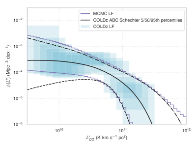
Figure 1: Illustrations of the fiducial model ensemble for CO(1–0) emission at $z\sim 3$. Upper left: The model parameter posterior distribution from the MCMC combining our priors (red dashed lines in marginalized posterior plots) with a likelihood based on the COLDz ABC constraints. Upper right: The luminosity function posterior distribution calculated from the MCMC. We show 90% intervals for the MCMC (purple), the COLDz direct constraints (cyan shaded rectangles), and the COLDz ABC constraints on a Schechter luminosity function (black dashed, solid, and dash-dotted showing 5%, 50%, and 95% percentiles). Lower left: The 90% interval for $L(M_{h})$ from the MCMC, with the relation given by the parameter values of Equations 27–31 overplotted. Lower right: Predictions from the MCMC for the CO(1–0) $P(k)$. We compare the 68% interval from the MCMC (purple shaded area) to the fiducial model of Li et al. (2016) at $z=2.4$ (blue) and to the direct measurement from COPSS (cyan), as well as estimates based on mmIME data plus either the fiducial $r_{31}$ used by Keating et al. (2020) (green) or the Riechers et al. (2020) value based on VLASPECS follow-up (red).

Our MCMC output is a fiducial sample of models that we can use to validate models of line broadening across a reasonable range of $L(M_{h})$ parameter values. The posterior distribution is shown in Figure 1, as are the empirically derived MCMC priors for comparison in the marginalized posterior plots. The COLDz data significantly constrain the characteristic mass and luminosity scales $M_{1}$ and $C$ beyond our priors, as well as put meaningful limits on the power-law slopes $A$ and $B$. We strongly favour a super-linear $L(M_{h})$ relation at the faint end, with the power-law break point determined by $\log{C}\in(9.9,11.4)$ and $\log{(M_{1}/M_{\odot})}\in(11.8,13.1)$ (both 90% marginalized intervals).

We also show the 90% intervals for the CO luminosity function and $L(M_{h})$ relation. Alongside the luminosity function interval, we also show the COLDz results from Riechers et al. (2019), both as direct constraints on the luminosity function and as an approximate Bayesian computation (ABC) of constraints on a Schechter function description of the luminosity function. (Note that our MCMC likelihood function was based on the latter.) Our MCMC interval matches both quite well, although our interval favours a steeper faint-end luminosity function compared to the COLDz ABC constraints.

Although the inference is done at $z\approx 2.4$, we apply the parameters without change to the COMAP central redshift of $z\approx 2.8$ as we do not expect much evolution in cosmic star-formation activity between these redshifts. Any evolution would be subdominant to model uncertainties, so a sample of models that would be likely realistic for $z\approx 2.4$ would largely be equally likely realistic for $z\approx 2.8$ given our low level of information about high-redshift CO(1–0) emission. We will also revert from the Planck Collaboration XIII (2016) cosmology to the fiducial cosmology for this work without altering our model values, as again uncertainties in cosmology are far subdominant to model uncertainties.

For reference, when we tune our $L(M_{h})$ parameters to make the model $P(k)$ and luminosity function at $z\approx 2.8$ approximately match the median $P(k)$ and luminosity function from our MCMC posterior distribution (again, found originally at $z\approx 2.4$), the resulting representative set of parameters is as follows:

$$A =-2.75,$$ (27)

$$B =0.05,$$ (28)

$$\log{C} =10.6,$$ (29)

$$\log{(M_{1}/M_{\odot})} =12.3,$$ (30)

$$\sigma_{L} =0.42.$$ (31)

We show the relation based on these parameters alongside the 90% MCMC interval for $L(M_{h})$. The above parameters result in a $L(M_{h})$ relation slightly more optimistic than the median (reflected mostly by the relatively low value of $M_{1}$), which is a counter-reaction to the slight downward shift of the halo mass function when moving from $z\approx 2.4$ to $z\approx 2.8$. However, the figure shows that the resulting $L(M_{h})$ from the above parameter values still falls well within the 90% sample interval. This should demonstrate that any shift in our best estimate between these two redshifts is subdominant compared to the model uncertainties involved.

We also compare our model distribution of the real-space $P(k)$ to the fiducial model of Li et al. (2016) previously used for COMAP forecasts, as well as the current extent of CO intensity mapping measurements from COPSS and mmIME. In particular, the mmIME $z\sim 2.5$ estimate is converted from an estimate of CO(3–2) shot noise, and Keating et al. (2020) use a line-luminosity ratio $r_{31}=L^{\prime}_{\text{CO(3--2)}}/L^{\prime}_{\text{CO(1--0)}}$ from Daddi et al. (2015) of $0.42\pm 0.07$. However, this is an average based on three near-IR selected ‘normal’ star-forming galaxies at $z=1.5$. Meanwhile, follow-up of CO(3–2) detections from ASPECS (González-López et al., 2019) by the VLA-ALMA SPECtroscopic Survey (VLASPECS) in the Hubble Ultra-Deep Field (Riechers et al., 2020) resulted in three robust CO(1–0) detections for which the line ratios were found to be closer to 0.8–1.1, the best overall estimate being $r_{31}=0.84\pm 0.26$. Therefore, we show the mmIME result both with the fiducial $r_{31}$ from Daddi et al. (2015) used by Keating et al. (2020) and with the higher $r_{31}$ value from Riechers et al. (2020), to illustrate the level of uncertainty around the conversion from CO(3–2) to CO(1–0).

Our new model tends to predict higher shot noise and a dimmer clustering signal compared to Li et al. (2016), and is also in some tension with the COPSS result. However, our predictions are very consistent with the mmIME results, particularly if the applicable $r_{31}$ value is higher than the value used by Keating et al. (2020). That said, we do caution that neither of the experimental results include corrections for line broadening, which is the very effect we are setting out to describe.

3.2 Halo Mass–Line FWHM Relation

Various classes of galaxies demonstrate well-measured correlations between galaxy luminosity and velocity scales—between luminosity and rotation velocity in disk galaxies as first identified by Tully & Fisher (1977), or between luminosity and velocity dispersion in elliptical galaxies as first identified by Faber & Jackson (1976). However, measuring such correlations requires fine observations across many galaxies of line profiles as well as morphology and inclination, which is easier in the local Universe than at $z\gtrsim 2$.

Because we have comparatively limited information about the CO(1–0) line profiles of high-redshift galaxies, we will define our $v(M_{h})$ model in two steps. We first examine the line FWHM in observations to consider $v(M_{h})$ for sources around or brighter than the knee of the luminosity function—which broadly speaking should correspond to the characteristic mass and luminosity scales of our double power-law $L(M_{h})$—and then consider how best to extrapolate to lower $M_{h}$ where we have no information.

3.2.1 Average Line FWHM at Characteristic Mass

While current constraints on the double power-law slopes are limited, observations do sufficiently probe the knee of the $z\gtrsim 2$ CO luminosity function for information about the characteristic mass and luminosity scales at the double power-law break point, as we have already noted. Since observations identify individual line candidates with associated integrated line fluxes and line FWHM values, we can use these to get an approximate correspondence between CO luminosity and line FWHM, and in turn between halo mass and line FWHM, at these characteristic mass/luminosity scales.

To be clear, this is not a correlation we expect to be statistically very strong—the connection between halo properties and molecular gas dynamics is highly indirect, and we expect CO line FWHM for a given host halo mass to be highly variable. However, even an idea of the average CO line FWHM at a characteristic halo virial mass would help us model line broadening in a way acceptable at the $P(k)$ and VID level, where many emitters are sampled simultaneously and thus the variability may not be as relevant as in the context of scanning for individual line candidates.

As when formulating the MCMC likelihood used in our $L(M_{h})$ model above, we only consider CO-selected observations of CO(1–0) and no observations of higher-$J$ CO lines. Of the surveys mentioned in Section 3.1, the COLDz survey found four secure line candidates at $z\sim 2$–3 (Pavesi et al., 2018), and Riechers et al. (2020) reported three secure CO(1–0) line detections from VLASPECS as previously discussed. Table 1 lists these seven lines and their properties.

For the sources from Pavesi et al. (2018), we convert the integrated line flux $S\,\Delta\nu$ to the observed line luminosity $L^{\prime}$, via this relation (as found in, e.g., Solomon et al. 1992):

$$L^{\prime}=\frac{c^{2}}{2k}(S\,\Delta\nu)\frac{D_{L}^{2}}{\nu_{\text{obs}}^{2}(1+z)^{3}}.$$ (32)

In a flat universe as described by our fiducial cosmology, the luminosity distance is simply the comoving distance $R(z)$ divided by the scale factor; since $\nu_{\text{obs}}=\nu_{\text{rest}}/(1+z)$ is the rest-frame line frequency multiplied by the scale factor,

$$L^{\prime}=\frac{c^{2}}{2k}(S\,\Delta\nu)\frac{(1+z)R^{2}(z)}{\nu_{\text{rest}}^{2}}.$$ (33)

With $\nu_{\text{rest}}=115.26$ GHz for CO(1–0), this equation becomes

$$\frac{L^{\prime}_{\text{CO(1--0)}}}{\text{K\,km\,s}^{-1}\text{ pc}^{2}}=2.45\times{10}^{3}(1+z)\left(\frac{R(z)}{\text{Mpc}}\right)^{2}\frac{S\,\Delta\nu}{\text{Jy\,km\,s}^{-1}}.$$ (34)

Table 1: Properties of compiled secure CO(1–0) line detections at $z\sim 2$–3.

ID	Redshift	Line FWHM	$L^{\prime}_{\text{CO(1--0)}}$	Reference
		(km s-1)	(${10}^{10}$ K km s-1 pc2)
COLDz.COS.1	2.6675	$430\pm\phantom{0}80$	$\phantom{0}3.68\pm 0.10$	Pavesi et al. (2018)
COLDz.COS.2	2.4771	$830\pm 130$	$\phantom{0}3.83\pm 0.09$	Pavesi et al. (2018)
COLDz.COS.3	1.9692	$240\pm\phantom{0}50$	$\phantom{0}7.27\pm 1.97$	Pavesi et al. (2018)
COLDz.GN.3	2.4877	$580\pm 120$	$10.08\pm 3.56$	Pavesi et al. (2018)
ASPECS-LP.9mm.1	2.5437	$447\pm 110$	$\phantom{0}3.22\pm 0.68$	Riechers et al. (2020)
ASPECS-LP.9mm.2	2.6976	$201\pm\phantom{0}47$	$\phantom{0}1.32\pm 0.19$	Riechers et al. (2020)
ASPECS-LP.9mm.3	2.6956	$560\pm 230$	$\phantom{0}3.14\pm 0.75$	Riechers et al. (2020)

Note. — Pavesi et al. (2018) provide $S\,\Delta\nu$ rather than $L^{\prime}_{\text{CO(1--0)}}$; the main text explains how we calculate the latter from the former. Riechers et al. (2020) provide the $L^{\prime}_{\text{CO(1--0)}}$ values shown above, and use a fiducial cosmology sufficiently similar to ours that we do not re-calculate luminosities.

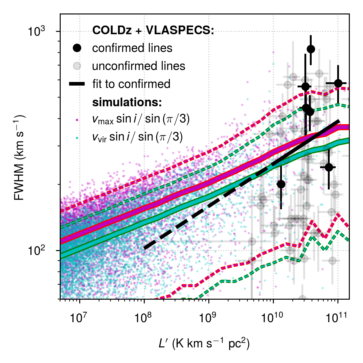
Figure 2: Plot of line luminosity $L^{\prime}$ against line FWHM for the seven sources (black points with error bars) described in Table 1, along with the power-law fit (black solid line) described in the main text. We also show unconfirmed line candidates (grey points with error bars) from Pavesi et al. (2018) and Riechers et al. (2020), with no attempt made to correct for any magnification. We show the inclination-adjusted FWHM estimated from $v_{\text{vir}}$ (cyan) and $v_{\text{max}}$ (magenta) for a random subset (to avoid overcrowding the plot) of the halo catalogue of a sample lightcone from simulations detailed in Section 6, with $L^{\prime}$ calculated based on the fiducial model with representative values from Equations 27–31, again assuming no magnification. We also show 90% intervals for both velocities (cyan and magenta dashed lines) at each $L^{\prime}$, to more clearly show the difference in the scaling of velocity with $L^{\prime}$ versus our naïvely extrapolated power-law fit (black dashed).

A fit across all seven line candidates to a power-law model, such that

$$\log{\frac{\text{FWHM}}{\text{km\,s}^{-1}}}=\delta_{0}+\delta_{1}\log{\frac{L^{\prime}}{10^{10}\text{ K\,km\,s}^{-1}\text{ pc}^{2}}},$$ (35)

finds $\delta_{0}=2.395\pm 0.208$ and $\delta_{1}=0.193\pm 0.302$. We show the fit graphically in Figure 2. While the correlation is not statistically significant, it is broadly consistent with the ‘spherical’ and ‘disk’ model $L^{\prime}$–FWHM relations of Aravena et al. (2019), which are examples given for comparison with estimated CO(1–0) luminosities based on higher-$J$ CO lines observed by ASPECS, and correspond to $\delta_{0}=2.14$ or 2.56 (for ‘spherical’ and ‘disk’ respectively) and $\delta_{1}=0.5$ (for both). Our fit is also consistent with correlations found from targeted observations of sub-millimetre galaxies. Harris et al. (2012), for instance, find a fit equivalent to $\delta_{0}=2.33$ and $\delta_{1}=0.59$ based on CO(1–0) observations only, and Goto & Toft (2015) find a fit equivalent to $\delta_{0}=2.52$ and $\delta_{1}=0.24$ also incorporating higher-$J$ observations.

Note that both Harris et al. (2012) and Goto & Toft (2015) find an intrinsic luminosity by dividing $L^{\prime}$ by the magnification $\mu$ in the presence of a gravitational lens where known, but such information is not available for the line candidates from Pavesi et al. (2018) or Riechers et al. (2020). Our assumption in formulating the $L(M_{h})$ model has been that $\mu=1$, and if we did not believe this then we would replace $L^{\prime}$ with $L^{\prime}/\mu$ in the right-hand side of Equation 22. We will assume that $\mu\approx 1$ for the sources in Table 1, although we caution that three of the seven sources do show at least marginally resolved spatial extension.

Note also the lack of information on the inclination angle $i$ of the CO emitter’s axis of rotation (with respect to the observer’s line of sight), which would scale the line profile by $\sin{i}$. The assumption that sources are randomly oriented corresponds to a uniform distribution of $\cos{i}$, such that the observed line FWHM is scaled down from the intrinsic rotation-dominated line FWHM by a median multiplier of $\sqrt{3}/2\approx 0.866$, and by no less than a multiplier of $1/2$ in $\approx 86.6$% of cases. Therefore, we will not consider any explicit corrections to the average $v(M_{h})$ based on $i$, given the lack of information in high-redshift observations.

We will in fact incorporate random $i$ in the detailed simulations presented in Section 6, as shown in Figure 2. But reflecting the absence of any corrections for $i$ in the above work, we will use a correction of $\sin{i}/0.866=\sin{i}/\sin{(\pi/3)}$ rather than $\sin{i}$ by itself, so that the correction is relative to the median adjustment for inclination. The implicit assumption here is that all of our emitters are disc-like or at least primarily rotationally supported; we will address this issue further in Section 3.2.3.

We also note that there are more unconfirmed line candidates from both Pavesi et al. (2018) and Riechers et al. (2020), which we partially show in grey in Figure 2. Given that the $z\sim 3$ CO(1–0) identification presumed for all of the unconfirmed line candidates is not definitive and other potential biases exist in flux or luminosity recovery, we will not present a fit using both secure and unconfirmed line candidates. Designing a procedure to infer a $L^{\prime}$–FWHM relation while accounting for source fidelity (as COLDz or ASPECS would in inferring the luminosity function) is beyond the scope of this paper.

In any event, our own fit suggests that on average, assuming negligible magnification for our secure line candidates, CO emitters with $M_{h}=M_{1}$ and thus $\log{L^{\prime}}$ in a fiducial 90% confidence interval of ${\log{(C/2)}\in(9.6,11.1)}$ should have line FWHM values in the range of 210–400 km s^-1, with the log-space midpoint at around 290 km s^-1.

How does this compare to the virial velocity expected from a halo with virial mass in our 90% confidence interval of $\log{M}\in(11.8,13.1)$? This mass range corresponds to a virial velocity range of approximately 200–540 km s^-1, with the log-space midpoint at 330 km s^-1. Therefore, at the double power-law break point, we find that the FWHM of a CO line profile approximately lines up with the virial velocity of its host dark matter halo.

The virial velocity $v_{\text{vir}}$ and maximum circular velocity $v_{\text{max}}$ of a halo are typically within a factor of order unity of each other. We suppose that the maximum circular velocity calculated by the halo finder, given that it reflects halo dynamics, may best reflect dynamics associated with the hosted molecular gas. If both velocities are available, $v_{\text{max}}$ takes precedence as the FWHM for our simulated CO line profiles.

That the maximum circular velocity of the overall mass profile should be equal to the full width of the CO line profile, as opposed to the velocity dispersion (smaller than the FWHM by a factor of $2\sqrt{2\ln{2}}\approx 2.355$), is not unreasonable. While the velocity dispersion of atomic hydrogen is usually similar to that of matter (chiefly dark matter) for the $M_{h}>10^{10}\,M_{\odot}$ halo population that we consider (see, e.g., Figure 13 of Villaescusa-Navarro et al. 2018), the distribution of molecular gas in a galaxy is considerably more compact even than that of atomic gas, let alone matter in general. As a result of this compactness, CO profiles take on a shape closer to a Gaussian than the double-horned profile typical of 21 cm line emission, and are also likely to trace velocity widths at $\sim 2.5\times$ smaller radii than 21 cm profiles, resulting in line FWHM values smaller by up to a similar factor (de Blok & Walter, 2014).

Before we move to prescribe the line FWHM for all halo masses, note that our model of the galaxy–halo connection does not specify a non-trivial halo occupation distribution (HOD). While we make the very simple assumption of one CO emitter per halo in this work, explicitly assigning multiple CO emitters to a high-mass halo would somewhat push down the simulated values of $L^{\prime}$ for each emitter, allowing us to better explain some of the higher-FWHM line candidates from COLDz and VLASPECS shown in Figure 2. While we consider a HOD model for CO emitters to be beyond the scope of this paper, it could be an important consideration for future work due to these sorts of effects on the contribution of high-mass halos to the simulated CO signal.

3.2.2 Average Line FWHM at All Halo Masses

The above work makes a case—if a highly tentative one—that at the double power-law break point specifically, the FWHM of the CO emitter line profile is approximately equal to the host halo maximum circular velocity (or virial velocity, largely similarly). However, this still raises the question of how the CO line FWHM scales on average away from this characteristic scale.

If we were to extrapolate the fit between FWHM and $L^{\prime}$ to lower $L^{\prime}$, it would suggest that the line FWHM scales approximately as $L^{\prime 1/5}$. Our priors are consistent with fairly sharp $L(M_{h})$ scalings at the faint end like $L^{\prime}\sim M_{\mathrm{vir}}^{2.5}$, which suggests that the line FWHM would scale almost as the square root of the host halo mass. By contrast, the circular velocity approximately scales as $M_{\mathrm{vir}}^{1/3}$ on average, which is a fairly weak scaling. Figure 2 illustrates how circular velocity (virial or maximum) scales more weakly with $L^{\prime}$ than the extrapolated FWHM fit.

However, we will adopt the more conservative prescription that even at lower halo mass, the CO line profile FWHM is equal (again, on average, specifically for the median inclination angle of $\pi/3$) to the halo maximum circular velocity. This reflects not necessarily high confidence in this prescription per se, but rather the low amount of information we have about high-redshift CO. Our simulations include emitters with luminosities several orders of magnitude below the double power-law break point; therefore, strictly in principle, extrapolation of a fit across points that barely span one order of magnitude in $L^{\prime}$ is unsafe in comparison to the assumption that rotation of molecular gas in a galaxy will scale with host halo mass in roughly the same way as the host halo’s rotation.

Furthermore, for a sufficiently faint CO emitter (or light host halo), the velocity dispersion of the CO gas itself will begin to dominate over rotational dynamics, weakening any scaling of FWHM with host halo mass. Our assumed minimum luminous host halo mass is $M_{\text{vir}}=10^{10}\,M_{\odot}$, corresponding to a virial velocity of approximately 50 km s^-1—roughly equal to the expected gas velocity dispersion for high-redshift galaxies (de Blok & Walter, 2014).

3.2.3 Additional Notes on Inclination and Scatter

We noted above that we will assume CO emitters are randomly oriented and that this reduces the observed line FWHM by the sine of the inclination angle relative to the FWHM for an edge-on emitter. Introducing this random inclination angle for all emitters raises the question of whether we ought to assume CO emitters at $z\sim 3$ are rotation-dominated, as such corrections for inclination should not apply to dispersion-dominated galaxies where random motions of molecular gas rather than galactic rotation contribute to most of the observed line profile.

So far we have made use of data from direct observations of CO(1–0) lines, but it is challenging to study kinematics across large numbers of such sources given the spatial resolution required and the long wavelength. Even looking to slightly higher-$J$ lines, blind line searches like ASPECS—which perhaps provide some of the larger samples of CO-selected galaxies in the literature—are not well-suited for kinematic studies as sources are spatially only marginally resolved. (That said, some CO-selected ASPECS sources do show clear rotation-dominated velocity gradients—see Appendix D of Aravena et al. 2019.)

As this cosmic epoch shows much greater star-formation activity compared to $z\sim 0$, with a much more dominant interstellar gas component for fuel, there is a good reason to suspect that the fraction of rotation-dominated galaxies is much smaller than in the local universe. Targeted studies of ionized gas kinematics across large numbers of star-forming galaxies at $z\gtrsim 1$ suggest that indeed at high redshift, rotation-dominated galaxies are far from an overwhelming majority. For example, Wisnioski et al. (2019) find a steadily declining fraction of rotation-dominated galaxies from 91% at $z\sim 1$ to 70% at $z\sim 2$, and Turner et al. (2017) find an even lower fraction of $34\pm 8$% at $z\sim 3.5$.

It is safe to assume that similar physical considerations apply for molecular gas, so a naïve prescription would be to model a rotation-dominated inclination-adjusted line profile for half of our CO emitters, and model a dispersion-dominated inclination-independent line profile for the other half. But it is not immediately clear that this is the correct tack to take. Depending on the exact criteria for deciding that a galaxy is ‘rotation-dominated’, the circular rotation may still be a significant even if not dominant source of support for its dynamical mass, and thus a significant contributor to the line profile width.

Furthermore, while the works discussed above find a less-than-overwhelming majority of galaxies to be rotation-dominated, ground-based near-infrared observations of ionized gas are often susceptible to spatial resolution effects that mask lower rotation velocities, leading to smaller rotation-dominated systems being classified as dispersion-dominated. The work of Newman et al. (2013) provides a striking illustration of the effect with a sample of $z\sim 2.2$ galaxies, where of 34 galaxies observed with adaptive optics, seeing-limited data would lead to 41% being classified as dispersion-dominated, but using higher-resolution adaptive optics data would drop this fraction to 6–9%. Although kinematics studies like Turner et al. (2017) and Wisnioski et al. (2019) will always attempt to correct for beam smearing, observational classification of galaxies as rotation- or dispersion-dominated is still far richer with complexities than the apparent simple binary would suggest at first glance.

Overall, there are not enough observational data—certainly not directly in CO lines—to advise against the assumption that a majority of CO emitters at $z\sim 3$ are rotationally supported, at least somewhat disc-like systems. So for the remainder of this work, when we apply inclination corrections, we will apply them to all simulated emitters.

Note that the random inclination angles assigned to each emitter will be the only source of random scatter in $v(M_{h})$. While for $L(M_{h})$ we introduce random log-normal scatter on top of the average relation described by $\sigma_{L}$, we will not take similar steps for $v(M_{h})$, or at least not explicitly through a parameter analogous to $\sigma_{L}$. The already-specified scatter in $L(M_{h})$ actually accounts for much of the observed variation in FWHM given $L^{\prime}$ for high-redshift CO emitters. Variations due to random inclination are smaller and skewed, but sufficient to account for any remaining variation (as possibly seen when including unconfirmed line candidates in Figure 2). Beyond these two sources of scatter, we find insufficient information to support any empirically motivated non-specific scatter (log-normal or otherwise) in FWHM for fixed halo mass and redshift in the way we do for $L(M_{h})$.

4 Possible Simplifications

Taking all of the above into account, with infinite computing time and space available to us, we would simulate line broadening in lightcones from cosmological N-body simulations by simulating a Gaussian line profile for each individual halo, taking the halo $v_{\text{max}}$ as the line width. Given the typical halo count ($\sim 10^{6}$) in a simulated COMAP survey volume, this is infeasible. A more efficient approach would be binning in halo mass and applying Gaussian filters based on an average $v_{\text{max}}$ to the CO map generated from each mass bin. However, for a meaningful number of mass bins ($\sim 100$), even this is too computationally expensive to be incorporated into a MCMC step that would complete within a reasonable amount of time. Furthermore, if we were to follow Ihle et al. (2019) and use approximate N-body simulations provided by the peak-patch method (Stein et al., 2019), which do not in their current state provide halo properties like $v_{\text{max}}$, we would have to rely on calculations based on halo mass.

Therefore, we will consider some approaches that will use $v_{\text{vir}}(M_{h})$ and make further simplifications. One approach is to use a single Gaussian filter with an effective velocity scale $v_{\text{eff}}$ to describe the broadening of the total CO line-intensity cube. This comes at the cost of some accuracy, but would bring significantly improved computational speed in any contexts where the approximation is applicable. The goal of Section 4.1 is to obtain a prescription for $v_{\text{eff}}$ that results in the same $P(k)$ attenuation as a simulation with halo mass bins broadened by $v_{\text{max}}$, to within $\sim 10$% up to $k=0.7$ Mpc^-1 (beyond which attenuation of $P(k)$ due to the COMAP angular beam will exceed 50%, even without any line-of-sight smearing). We then consider an alternate approach in Section 4.2 that still uses multiple bins in $v_{\text{vir}}$ but designs these bins more carefully to reduce the number of bins required and thus reduce computational burden.

4.1 Use of a Single Effective Line Width

A description of line broadening using a single effective line width is extremely desirable as long as it achieves a reasonable accuracy. If we can design such a $v_{\text{eff}}$, we could treat the corresponding $\sigma_{\parallel,\text{eff}}$ the same way as the mass-independent $\sigma_{\parallel}$ in Equation 9. This would in turn drastically simplify the computational work involved compared to the full calculation described in Equation 13 and Equation 20. In a simulation using dark matter halo catalogues, the only necessary step to incorporate line broadening would be to apply a single Gaussian filter along the line of sight with its profile given by $v_{\text{eff}}$, as opposed to creating dozens of mass or velocity bins with individual profile widths.

To design $v_{\text{eff}}$, we focus on the shot-noise component of the power spectrum. Not only is attenuation stronger at higher wavenumbers—where the shot noise dominates $P(k)$—but also the emitters that contribute most to shot noise will tend to see greater line broadening.

Concentrating on shot noise attenuation allows us to state the problem in mathematical terms. A Gaussian line profile with FWHM of $v_{\text{FWHM}}$ in velocity units can be translated into a Gaussian profile in comoving space, with the standard deviation given by the same relation as Equation 12,

$$\sigma_{\parallel}(v_{\text{FWHM}})=\frac{(1+z)}{H(z)}\frac{v_{\text{FWHM}}}{2\sqrt{2\ln{2}}}.$$ (36)

The virial velocity $v_{\text{vir}}$ is quite close to $v_{\text{max}}$—a visual inspection of Figure 2 suggests they fall within 20% of each other. But unlike $v_{\text{max}}$, $v_{\text{vir}}$ is explicitly a function of the halo virial mass $M_{h}$ and redshift $z$:

$$v_{\text{vir}} =\sqrt{\frac{GM_{h}}{r_{\text{vir}}}}=\left(\frac{\Delta_{c}}{2}\right)^{1/6}\left[GM_{h}H(z)\right]^{1/3}$$ (37)

$$\approx 35\text{\,km\,s}^{-1}\left(\frac{\Delta_{c}}{200}\right)^{1/6}\times$$

$$\qquad\left(\frac{M_{h}}{10^{10}\,M_{\odot}}\frac{H(z)}{100\text{\,km\,s}^{-1}\text{\,Mpc}^{-1}}\right)^{1/3},$$ (38)

where $\Delta_{c}$ is the spherical overdensity relative to the critical density $\rho_{\text{crit}}$, and thus relates the virial mass and radius:

$$r_{\text{vir}}=\left(\frac{3M_{h}}{4\pi\Delta_{c}\rho_{\text{crit}}}\right)^{1/3}=\left(\frac{2GM_{h}}{\Delta_{c}H^{2}(z)}\right)^{1/3}.$$ (39)

We use the definition of $\Delta_{c}$ and thus virial mass from Bryan & Norman (1998), which yields $\Delta_{c}\approx 180$ for our cosmology and redshift. For reference, $H(z)$ at the central COMAP redshift is approximately $290\text{\,km\,s}^{-1}\text{\,Mpc}^{-1}$.

We can convert $v_{\text{vir}}(M_{h})$ into the comoving $\sigma_{v}(M_{h})$ expected for a CO emitter with host halo mass $M_{h}$ using Equation 12. We would then feed this into Equation 13 and integrate in $\mu$ to carry out a full calculation of the shot noise with line broadening.

Compare to using a single mass-independent velocity scale $v_{\text{eff}}$, with corresponding $\sigma_{\parallel,\text{eff}}=\sigma_{\parallel}(v_{\text{eff}})$. Based on Equation 22 of Chung (2019), considering only the line-of-sight attenuation, the observed shot noise is the true $P_{\text{shot}}$ multiplied by

$$S_{0}=\frac{\pi^{1/2}\operatorname{erf}{(k\sigma_{\parallel,\text{eff}})}}{2k\sigma_{\parallel,\text{eff}}}.$$ (40)

Then we want to identify $v_{\text{eff}}$ such that

$$\frac{\pi^{1/2}\operatorname{erf}{(k\sigma_{\parallel,\text{eff}})}}{2k\sigma_{\parallel,\text{eff}}}$$

$$=\frac{\int_{0}^{1}d\mu\int dM_{h}\,dn/dM_{h}\,L^{2}(M_{h})\exp{[-k^{2}\mu^{2}\sigma_{v}^{2}(M_{h})]}}{\int dM_{h}\,dn/dM_{h}\,L^{2}(M_{h})}.$$ (41)

We intentionally ignore the angular resolution of the survey so as to devise $v_{\text{eff}}$ as a well-defined function of the $L(M_{h})$ and $v(M_{h})$ models alone. We will see that this affects the fidelity of this approximation when $\sigma_{\perp}$ is non-negligible.

We can clearly solve Equation 41 exactly for $\sigma_{\parallel,\text{eff}}$ at each $k$, at least numerically. However, we want to find a single velocity scale $v_{\text{erf}}$ that approximately satisfies Equation 41 across all $k$. In other words, for all $k$, $\sigma_{\parallel,\text{erf}}=\sigma_{\parallel}(v_{\text{erf}})$ satisfies

$$\frac{\operatorname{erf}{(k\sigma_{\parallel,\text{erf}})}}{k\sigma_{\parallel,\text{erf}}}\approx\frac{\left\langle{L^{2}\text{erf}{\left[k\sigma_{v}(M_{h})\right]}/[k\sigma_{v}(M_{h})]}\right\rangle}{\left\langle{L^{2}}\right\rangle},$$ (42)

where $\left\langle{x}\right\rangle\equiv\int dM_{h}\,(dn/dM_{h})\,x$. So for any given set of model parameters fully determining $L(M_{h})$, we can calculate the shot noise transfer function across $k$ on the right-hand side and solve numerically for the $\sigma_{\parallel,\text{erf}}$ corresponding to that parameter set.

Rather than repeatedly solving for $v_{\text{erf}}$ (which comes with issues of reliability and computational cost), we want a closed-form quantity that we can calculate from the analytic halo model. Since the shot noise is the second moment of the luminosity function, a reasonable starting point for a representative velocity scale is the $L^{2}$-weighted average $v_{\text{vir}}$. Again using $\left\langle{x}\right\rangle\equiv\int dM_{h}\,(dn/dM_{h})\,x$, we might write

$$v_{\text{eff}}\stackrel{{\scriptstyle?}}{{=}}\frac{\left\langle{L^{2}v_{\text{vir}}}\right\rangle}{\left\langle{L^{2}}\right\rangle}.$$ (43)

However, note that $\operatorname{erf}{x}\to 1$ as $x\to\infty$, such that for very high $k$ we actually expect a more reasonable estimate to be the inverse of the $L^{2}$-weighted average $v^{-1}(M)$,

$$v_{\text{eff}}\stackrel{{\scriptstyle?}}{{=}}\frac{\left\langle{L^{2}}\right\rangle}{\left\langle{L^{2}v_{\text{vir}}^{-1}}\right\rangle}.$$ (44)

Ultimately, however, we will find that the best estimate for $v_{\text{erf}}$ is the average of these two estimates,

$$v_{\text{eff}}\equiv\frac{1}{2}\left(\frac{\left\langle{L^{2}v_{\text{vir}}}\right\rangle}{\left\langle{L^{2}}\right\rangle}+\frac{\left\langle{L^{2}}\right\rangle}{\left\langle{L^{2}v_{\text{vir}}^{-1}}\right\rangle}\right).$$ (45)

We can then use Equation 36 to convert this to a $\sigma_{\parallel}$ value, with which we can then use Equation 9 to calculate the power spectrum analytically or numerically, or set the appropriate scale for the Gaussian filter to apply to a mock CO cube.

We give a very loose theoretical justification for our choice in the context of a simplified model in Appendix B, but our main justification will be based on explicit numerical calculations comparing $v_{\text{erf}}$, $v_{\text{eff}}$, and our other ansätze across a broad range of model parameters in our fiducial distribution.

Note that the above calculation of $v_{\text{eff}}$ does not account for the effect of randomly distributed inclination angles. The effect can be expressed using special functions but the functions involved are more complex without necessarily yielding an improved qualitative understanding. Therefore, while we discuss explicit analytic derivations in Appendix A, here we will simply show the required adjustment, which is a slight decrease in the high-$k$ ansatz:

$$v_{\text{eff}}\equiv\frac{1}{2}\left(\frac{\left\langle{L^{2}v_{\text{vir}}}\right\rangle}{\left\langle{L^{2}}\right\rangle}+\frac{4}{\pi\sqrt{3}}\frac{\left\langle{L^{2}}\right\rangle}{\left\langle{L^{2}v_{\text{vir}}^{-1}}\right\rangle}\right).$$ (46)

4.2 Careful Design of Mass or Velocity Bins

Not all brute-force simulations are equally brute. While binning CO emitters according to mass or velocity and then applying Gaussian filters to each bin is the most straightforward and brute method of simulating line broadening that is still computationally feasible, carefully choosing the binning scheme should result in being able to maintain accuracy while saving computational cost.

In the case of our fiducial model, note that low-mass emitters (and thus narrow CO line profiles) will typically neither be resolvable in frequency space nor contribute significantly to the power spectrum at small scales where the effect of line broadening becomes marked. For instance, with CO(1–0) at $z\sim 3$, the dominant contribution to shot noise will be from $M_{h}\sim 10^{12}$ emitters with $v_{\text{vir}}\sim 230$ km s^-1. The COMAP science channelization of 15.6 MHz quoted in Ihle et al. (2019) ($156$ km s^-1 in velocity space) can resolve these profiles but not the profiles corresponding to emitters with $M_{h}\lesssim 10^{11}\,M_{\odot}$ (for which $v_{\text{vir}}\lesssim 100$ km s^-1).

The native instrumental frequency resolutions of COMAP ($\sim 2$ MHz) and mmIME ($4$–$8$ MHz) are signficantly finer than the $>10$ MHz binning applied during data analyses, and in principle the spectrometers used are capable of resolving widths of $\lesssim 100$ km s^-1. However, in practice such line profiles would not likely be detectable due to the low line intensity associated. Even in aggregate, the contribution of these low-mass (narrow-width) emitters to the power spectrum—particularly the shot-noise component of the power spectrum—would remain subdominant.

Then consider a CO simulation at $z\sim 3$ with halo masses ranging from $10^{10}\,M_{\odot}$ to $3\times 10^{13}\,M_{\odot}$. This corresponds to $v_{\text{vir}}\in(50,700)$ km s^-1, so a brute binning scheme might define equally spaced bins across this range. But one-sixth of these bins—not a majority of the bins, but not exactly a negligible fraction—will correspond to $M_{h}\in(10^{10},10^{11})\,M_{\odot}$. This population is about 100 times more numerous than the $M_{h}\gtrsim 10^{11}\,M_{\odot}$ population, yet negligible for the purpose of simulating the line broadening effect for the reasons that we have described above.

Therefore, a less-brute two-tier scheme will bisect the halo population in our simulation around $M_{h}=10^{11}\,M_{\odot}$, applying no line broadening to the low-mass subset but binning and applying line broadening to the high-mass subset. This reduces the need to iterate repeatedly through the low-mass but far more numerous halo subset, and also reduces the number of bins used without significantly lowering accuracy, which we will demonstrate in Section 6.

5 Preliminary Validation of Effective Line Width

While we will eventually simulate $z\sim 3$ CO(1–0) based on lightcones from dark matter simulations, we undertake a sanity check in this section with numerical calculations based on the above analytic halo model, in order to set expectations for accuracy of using $v_{\text{eff}}$ relative to the full calculation of line broadening, both before and after inclination corrections. In the first two subsections we will check $v_{\text{eff}}$ across a subset of our fiducial model distribution. Then in the final subsection, we will actually make a diversion outside of $z\sim 3$ CO(1–0) and examine line broadening of the CO lines at $z\sim 1$–5 observed by mmIME to show that our effective line width is a reasonable description of the effect on the monopole $P_{0}(k)$ consistent with the calculations in Appendix A of Keating et al. (2020).

5.1 Fiducial Model Ensemble

To check whether $v_{\text{eff}}$ from Equation 45 is a good description of the ideal $v_{\text{erf}}$ of Equation 42 (both before correcting for inclination effects), we take 1764 samples from the MCMC of Section 3.1 and fit for $v_{\text{erf}}$ (minimising the summed squared difference between the two sides of Equation 42 across all $k$) as well as calculate $v_{\text{eff}}$ and the other ansätze of $\left\langle{L^{2}v_{\text{vir}}}\right\rangle/\left\langle{L^{2}}\right\rangle$ and $\left\langle{L^{2}}\right\rangle/\left\langle{L^{2}v_{\text{vir}}^{-1}}\right\rangle$. We use the lim package as our basis for all calculations.

Figure 3: Comparison of effective line FWHM and ansätze before accounting for inclination. Upper panels: scatter plot of $v_{\text{erf}}$ for 1764 draws from our fiducial model posterior, against model parameters $A$ (left), $B$ (middle), and $M_{1}$ (right), illustrating correlations or lack thereof as described in the main text. Lower panels: scatter plot of the relative differences between our ansätze against the same three model parameters as in the upper panels, once again showing correlations or lack thereof.

We show the results in Figure 3. First it is useful to note the range of $v_{\text{erf}}$, which falls predominantly in the 200–500 km s^-1 range corresponding to the predominant range of $\log{(M_{1}/M_{\odot})}$. However, while there is a very strong correlation indeed between $v_{\text{erf}}$ and $M_{1}$, it is not perfect in our data. This appears to be in part due to outliers where $M_{1}$ is so low—below our minimum emitter $M_{h}=10^{10}\,M_{\odot}$, in fact—that we have effectively ended up with a single power-law description of $L(M_{h})$. There is however some additional scatter around the average correlation even at $M_{1}\gtrsim 10^{12}\,M_{\odot}$, part of which seems to be from a weak anti-correlation between $B$ and $v_{\text{erf}}$. We can explain this based on the fact that if $B<0$, the double power-law $L(M_{h})$ relation breaks into a shallower but still positive slope for $M_{h}>M_{1}$, and therefore the CO shot noise becomes dominated by very rare but very bright CO emitters.

Moving on to our ansätze, we find that $v_{\text{eff}}$ is extremely close to $v_{\text{erf}}$—the relative difference between the two is below 0.5% in the vast majority of cases. Meanwhile our other ansätze differ by larger fractions from $v_{\text{erf}}$, but somewhat astonishingly in opposite directions by almost exactly opposite amounts. Our best qualitative explanation for this is that $\left\langle{L^{2}v}\right\rangle/\left\langle{L^{2}}\right\rangle$ better describes attenuation at intermediate scales ($k\sim 1$ Mpc^-1) while $\left\langle{L^{2}}\right\rangle/\left\langle{L^{2}v^{-1}}\right\rangle$ describes attenuation at small scales ($k\gtrsim 1$ Mpc^-1) almost exactly. The midpoint $v_{\text{eff}}$ is a compromise between the two and will thus match up with the fit $v_{\text{erf}}$ which has to make a similar compromise.

The difference increases with lower values of $B$, where compared to $v_{\text{erf}}$ we find that $\left\langle{L^{2}v}\right\rangle/\left\langle{L^{2}}\right\rangle$ is too high and $\left\langle{L^{2}}\right\rangle/\left\langle{L^{2}v^{-1}}\right\rangle$ too low by several percent. This is likely due to the larger range of mass scales that contribute to the shot noise as $L(M_{h})$ monotonically increases rather than plateauing or declining. In these situations, $\left\langle{L^{2}}\right\rangle/\left\langle{L^{2}v^{-1}}\right\rangle$ actually probably still describes the attenuation at high $k$ more accurately, but the deviation at intermediate $k$ is likely greater and the relative difference from the fit $v_{\text{erf}}$ thus greater as well. We also find some correlation between relative differences and $M_{1}$ or $A$, although much of this may be driven by underlying weak correlations between the model parameters themselves.

In summary, we find that our $v_{\text{eff}}$ prescription is just as good as fitting $\operatorname{erf}{(k\sigma_{\parallel})}/(k\sigma_{\parallel})$ to the shot noise attenuation across ${k\in(10^{-2},10^{1})}$ Mpc^-1 and solving for $\sigma_{\parallel}$. However, do note that our ‘failed’ ansätze are actually still reasonable descriptions within a few percent in most cases, and in particular we still wholly expect $\left\langle{L^{2}}\right\rangle/\left\langle{L^{2}v^{-1}}\right\rangle$ to be the better effective line width to use at very high $k$.

Note that two key caveats apply to these last couple of points. One is that these facts only hold as long as angular resolution effects are comparatively negligible, since these were not included in devising that ansatz. The other caveat is that the relative errors across the ansätze will be much greater once we include corrections for inclination, as shown in Figure 4. That said, the qualitative points about the different ansätze still hold. This includes the point that $\left\langle{L^{2}}\right\rangle/\left\langle{L^{2}v^{-1}}\right\rangle$, or rather $4/(\pi\sqrt{3})\cdot\left\langle{L^{2}}\right\rangle/\left\langle{L^{2}v^{-1}}\right\rangle$, should be the best ansatz at very high $k$ in the absence of a sizeable angular beam. However, differences in functional form mean that the attenuation will asymptote less quickly to this description with inclination corrections than without them, meaning that errors may be so large for any scales relevant to actual power spectrum analysis that we may as well use the midpoint $v_{\text{eff}}$ instead. We will see this in Section 5.3 in our consideration of power spectra observed by mmIME.

Figure 4: Same as Figure 3 but after accounting for inclination.

5.2 A Closer Look at Attenuation for Specific Parameter Values

So far, we have looked at the shot noise attenuation in isolation. But it will be most instructive to examine the total $P_{0}(k)$ and $P_{2}(k)$, incorporating both clustering and shot-noise components and accounting for all redshift-space observational effects that we have discussed so far, including the effect of angular resolution in the context of a single-dish experiment like COMAP. This will come at somewhat increased computational cost, and we will be making equivalent calculations from N-body simulations later in this work. However, we will examine numerical realizations of our analytic model for two sets of parameter values, accounting for inclination throughout.

We first examine the effect of line broadening given the model parameter values given towards the end of Section 3.1 in Equations 27 through 31, which broadly represent the median expected $P(k)$ and luminosity function. This will give a sense of what our average expectation should be for attenuation of the total $P_{0}(k)$ and $P_{2}(k)$.

Figure 5: Illustration of the expected effect of line broadening on the $z\sim 3$ CO(1–0) $P_{0}(k)$ predicted by the model parameter values of Equations 27–31, both ignoring angular resolution (left panels) and assuming smearing with a Gaussian beam of FWHM $4.5^{\prime}$ or $\sigma_{\perp}=3.5\text{\,Mpc}$ (right panels). Upper panels: $P_{0}(k)$ calculated with the full formalism of Section 2 (inclination-inclusive; magenta dash-dotted) and with just $v_{\text{eff}}$ (orange). For the full calculation we also show the clustering (indigo dashed) and shot-noise (indigo dotted) contributions separately, and also show the unattenuated shot noise (black dashed) as a guide. Middle panels: Attenuation due to the introduction of line broadening, calculated using the full formalism, both without inclination corrections (magenta solid) and with them (cyan dotted). Lower panels: Error relative to the full calculation (with inclination corrections) from using each of our three ansätze for effective line width—$\left\langle{L^{2}v}\right\rangle/\left\langle{L^{2}}\right\rangle$ (blue dashed), $\left\langle{L^{2}}\right\rangle/\left\langle{L^{2}v^{-1}}\right\rangle$ (green dash-dotted), and the midpoint $v_{\text{eff}}$ (orange solid)—all inclination-inclusive.

We show the effect on $P_{0}(k)$ in Figure 5, first ignoring angular resolution and then accounting for the COMAP beam FWHM of $4.5^{\prime}$ at 30 GHz, which corresponds to $\sigma_{\perp}\approx 3.5$ Mpc. The overall conclusion is that using a single $v_{\text{eff}}$ results in a very good approximation of the attenuation of $P_{0}(k)$ for scales relevant to COMAP, but it is worth noting that when incorporating a non-zero $\sigma_{\perp}$—which our definition of $v_{\text{erf}}$ in Equation 42 does not—our approximation breaks down as we approach the comoving scales corresponding to the COMAP beam size ($\pi/\sigma_{\perp}\sim 0.9$ Mpc^-1). Indeed the high-$k$ ansatz of Equation 44 also fails because it too does not account for the presence of an angular beam.

The actual amount of $P_{0}(k)$ attenuation is also worth discussing briefly. While we defined $v_{\text{erf}}$ while ignoring angular resolution, the $P_{0}(k)$ attenuation from line broadening clearly must depend on beam smearing. Quantitatively, Equation 20 and Equation 13 show that the two effects are not separable into independent multipliers in front of the unattenuated power spectrum components. Qualitatively, the fact that beam smearing effectively discards angular modes means the spherical averaging of $P(k,\mu)$ into $P_{0}(k)$ must depend more heavily on line-of-sight modes, thus increasing the relative weight of line broadening in attenuation.

Nonetheless, these divergences between the cases of $\sigma_{\perp}=0$ and $\sigma_{\perp}\approx 3.5$ Mpc are somewhat esoteric in the context of the actual COMAP observation, where the very beam smearing that results in the breakdown of our approximation already introduces its own power loss in the same regime where this breakdown occurs. Given the transfer functions from both beam smearing and loss of large-scale modes due to filtering in the data pipeline prior to map-making—see Foss et al. (in prep.) for specific details—the COMAP $P_{0}(k)$ measurement will be most sensitive to $k\sim 0.2$–0.3 Mpc^-1. Therefore, in this case, line broadening should only introduce 7–8% attenuation of $P_{0}(k)$ at scales relevant to COMAP.

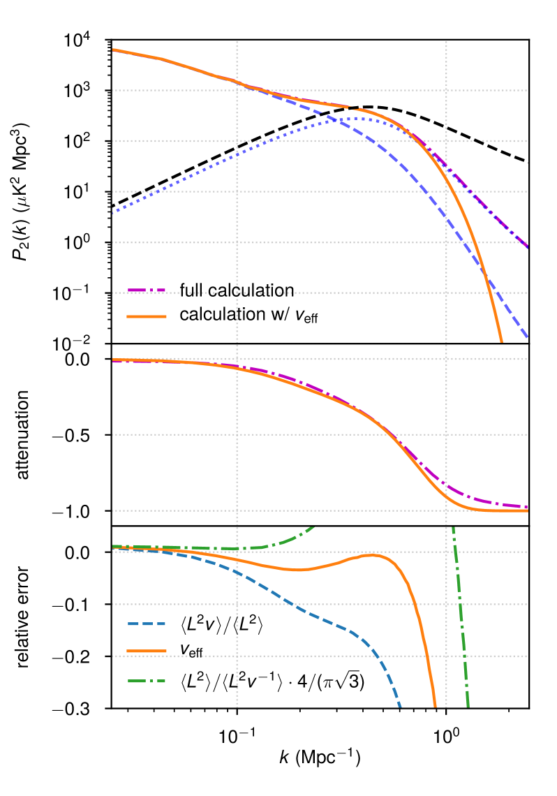
Figure 6: Similar to the right panels of Figure 5 (assuming smearing with a Gaussian beam of FWHM $4.5^{\prime}$ or $\sigma_{\perp}=3.5\text{\,Mpc}$), but showing attenuation of $P_{2}(k)$. The unattenuated shot-noise contribution to the quadrupole (black dashed) shown in the top panel is calculated after beam smearing is taken into account but before line broadening is applied.

We also show the effect of line broadening on the quadrupole $P_{2}(k)$ in Figure 6. Here, we only show the case where we set ${\sigma_{\perp}\approx 3.5}$ Mpc, as this is required (along with $\sigma_{\perp}>\sigma_{\parallel}$, which is the case here) for a positive shot-noise contribution to the quadrupole. The overall conclusions are similar to those for $P_{0}(k)$ in that the approximation breaks down near the COMAP beam scale but is otherwise acceptable. We do note however that the attenuation of the shot-noise component of the quadrupole due to line broadening is far more severe for even intermediate scales than it was for the monopole, at around 30% for $k\sim 0.2$–0.3 Mpc^-1.

We might naturally ask whether these conclusions still hold for a more extreme draw from our fiducial distribution with unusual values of $A$ or $B$. So we also show the same plots given the following parameter values:

$$A =-0.97,$$ (47)

$$B =-0.35,$$ (48)

$$\log{C} =11.1,$$ (49)

$$\log{(M_{1}/M_{\odot})} =12.8,$$ (50)

$$\sigma_{L} =0.5.$$ (51)

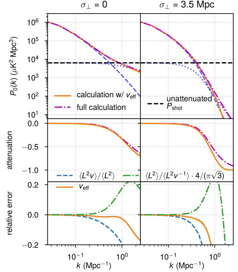
Figure 7: Same as Figure 5 but using the model parameter values of Equations 47–51, representing a more extreme draw from our distribution with a high value of $A$.

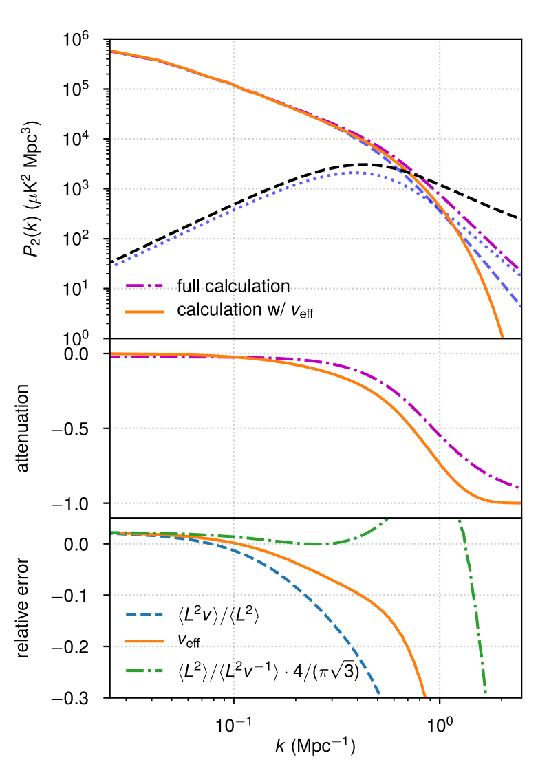
Figure 8: Same as Figure 6 but using the model parameter values of Equations 47–51.

We show $P_{0}(k)$ in Figure 7 and $P_{2}(k)$ in Figure 8 for these parameter values. Importantly, the clustering component is much higher relative to the shot-noise component than in our more pedestrian parameter set, which is not necessarily surprising given the high value of $A$ and thus the shallow faint-end $L(M_{h})$ relation. This has a series of implications for the accuracy of our $v_{\text{eff}}$ prescription because, as we noted when discussing Equation 20, the attenuation of the clustering component is weighted by $L(M_{h})$ at each $M_{h}$ and thus should be less than the attenuation of the shot-noise component (weighted by $L^{2}$) for a monotonically increasing $v(M_{h})$. Therefore, our error in estimating attenuation is greater than in Figure 5 and Figure 6, and we will always expect too much attenuation in these situations because our approximation is based on the shot-noise component.

Still, in scales relevant to COMAP analysis ($k\lesssim 0.5$ Mpc^-1), the relative error is typically within a few percent for the monopole (although greater for the quadrupole), and the amount of attenuation in the monopole is only around 3%. This is much smaller than the amount of attenuation given our previous parameter set, precisely because the clustering component is so much more dominant. So our approximation behaves worse but the attenuation being approximated is smaller, both for the same reason.

Importantly, however, the fact that our approximation breaks down at small scales with the introduction of a non-negligible $\sigma_{\perp}$ does not bode well for its performance with respect to the VID. We will examine the VID explicitly in further simulations to follow in this work.

Note that while we have not discussed the effect of accounting for inclination in these cases, we do show it graphically in LABEL:sec:extremedraw_noincli. The effect on the attenuation is quite small for scales relevant to COMAP, although less negligible for $P_{2}(k)$. Furthermore, the accuracy of using $v_{\text{eff}}$ to describe the attenuation is largely the same after accounting for inclination.

5.3 Beyond the Fiducial: Models for mmIME CO Observations at 100 GHz

We have now mentioned the Millimetre-wave Intensity Mapping Experiment, or mmIME (Keating et al., 2020), on several occasions. While mmIME will be using data from several community interferometers across a wide frequency range, the first analysis work of Keating et al. (2020) looks at data from the Atacama Large Millimetre-wave Array (ALMA) in compact configurations observing at 100 GHz. Being aware of the line broadening effect but not having a detailed model of it, the key step taken is avoidance by excluding modes above a certain $k_{\parallel}$ from the analysis. Specifically, using the lag coordinate $\eta$ (written implicitly in inverse frequency units of $\nu_{\text{obs}}^{-1}$), the excluded modes correspond to $\eta>500$, and since $\eta$ and $k_{\parallel}$ are related by

$$k_{\parallel}=2\pi\eta\cdot\frac{H(z)\nu_{\text{obs}}}{c(1+z)},$$ (52)

the threshold of $\eta=500$ is equivalent to $k_{\parallel}\approx 0.75$ Mpc^-1 for $z=2.5$, corresponding to the frame for CO(3–2) observations at 100 GHz. The cut is designed to exclude all modes of redshift-space comoving wavelength $8.4$ Mpc and below, which corresponds to 600 km s^-1 and below in velocity space. Since observations discussed in Section 3.2 have found line widths below this are typical, the cut is fairly conservative. At the same time, as Keating et al. (2020) note, the cut will not entirely eliminate suppression of power from line broadening. Line profiles are finite in extent and are not perfect periodic modes, so line profiles that are $\sim 300$ km s^-1 wide will still lead to some attenuation of $\eta<500$ modes.

Keating et al. (2020) do not explicitly correct for this attenuation, but do note that if the shot noise is dominated by CO emitters with line widths of $\sim 300$ km s^-1, the measurement is likely attenuated by $\sim 25\%$ and the necessary correction thus an upward shift by one-third. Here we will examine whether we are able to derive similar corrections with our own (inclination-inclusive) model.

First, we review the emission models for the CO lines observed by mmIME. In essence, the models use the basic flow of Li et al. (2016), relating halo mass to star-formation rate via Behroozi et al. (2013a, b), star-formation rate to IR luminosity via a simple scaling of $10^{10}\,L_{\odot}\,M_{\odot}^{-1}$ yr, and then IR luminosity to CO luminosity. Since Li et al. (2016) model only CO(1–0) emission at $z\sim 3$, the models of Keating et al. (2020) link IR and CO luminosities via fits found in Kamenetzky et al. (2016) from a broad sample of $z<1$ galaxies observed with Herschel. These models inform how much each line should contribute to the total measurement, and are scaled up uniformly in luminosity to match the mmIME data. We will consider the models without this final scaling as it should not affect any results concerning attenuation from line broadening.

For this section only we will change our cosmological parameters to match those of Keating et al. (2020), namely $\Omega_{m}=0.27$ instead of 0.286. However, as Keating et al. (2020) do not note all parameters that may affect predictions (the baryonic matter density fraction, for instance), we do not expect to perfectly reproduce the predictions of Keating et al. (2020) for line intensity. Nonetheless, we are able to recreate the $L(M_{h})$ for the various CO lines at 100 GHz, and are able to reproduce the $P_{\text{shot}}$ values for each line to within 10% (except for CO(5–4) at $z\sim 4.8$, where we fall within 20%).

Table 2: CO lines observed by Keating et al. (2020) at 100 GHz as part of mmIME, with redshifts, predictions for shot noise power, and our calculated (inclination-inclusive) $v_{\text{eff}}$ for each line.

Line	$z$	$P_{\text{shot}}$ from	$P_{\text{shot}}$ from	$v_{\text{eff}}$
		Keating et al. (2020)	this work
		($\mu$K2 Mpc3)	($\mu$K2 Mpc3)	(km s-1)
CO(2–1)	1.3	$100h^{-3}=292$	315	168
CO(3–2)	2.5	$160h^{-3}=466$	519	213
CO(4–3)	3.6	$\hphantom{1}80h^{-3}=233$	209	220
CO(5–4)	4.8	$\hphantom{1}20h^{-3}=58\hphantom{3}$	046	199

For $v(M_{h})$, we will actually use the exact same prescription as for CO(1–0) at $z\sim 3$, which is to set the line FWHM equal to the virial velocity. Partly this is because devising $v(M_{h})$ for each line at each redshift is well beyond the scope of this paper, but partly we also expect the same prescription to be a reasonable one for other high-redshift CO lines, at least in the absence of high information. Looking at the three sources in Riechers et al. (2020) robustly detected in CO(1–0), we find that their CO(1–0) line widths are consistent with their CO(3–2) line widths from González-López et al. (2019). Although we broadly expect higher-$J$ CO lines to have steeper gas density profiles due to the higher gas temperatures required for excitation of these lines, we do not expect this to be an overwhelmingly large effect for the lines observed by mmIME.

Thus, using essentially the same $v(M_{h})$ as in Section 3.2 (albeit with appropriate modifications for redshift and cosmology) but swapping out the $L(M_{h})$ models to match Keating et al. (2020), we can find $v_{\text{eff}}$ for each line. We show these values in Table 2 alongside our reproduced $P_{\text{shot}}$ values. Note that $v_{\text{eff}}$ tends to be lower at lower redshift—despite the continued growth of halo masses, the decline in star-formation activity after $z\sim 3$ means that the halo mass scales that dominate the CO shot noise are smaller for lower redshift.

While our $v_{\text{eff}}$ values are somewhat lower than the 300 km s^-1 expectation of Keating et al. (2020), the comparison is not exactly even because of our choice of profile shape. In Appendix A, Keating et al. (2020) consider a simple Gaussian profile, a double-Gaussian profile, and a top-hat profile, and find that the simple Gaussian profile results in the most attenuation. The difference in attenuation is at a $\sim 20$% level, but so is our difference in line widths. So our prediction of attenuation really should be broadly consistent with the $\approx 25$% expectation of Keating et al. (2020).

We calculate the expected effect of line broadening for each of the lines individually, and show this in Figure 9. Note that we set $\sigma_{\perp}=0$, since angular resolution does not have the same relevance in (visibility-space) interferometric power spectrum measurements that it does in (image-space) single-dish measurements like COMAP.

Figure 9: Illustration of the expected effect of line broadening on the individual lines observed by mmIME at 100 GHz (indicated above each column of panels), using the $L(M_{h})$ model reproduced from Keating et al. (2020) and our $v(M_{h})$ model. Upper panels: $P_{0}(k)$ calculated with the full formalism of Section 2 (magenta solid), including the effect of random inclinations. For the full calculation we also show the clustering (magenta dashed) and shot-noise (magenta dotted) contributions separately. We also show the unattenuated shot-noise contribution to the quadrupole (black dashed), as well as the expected $P_{0}(k)$ when restricting calculations to modes with $\eta<500$ (grey dashed) or $\eta<250$ (cyan dash-dotted). Middle panel: Attenuation due to the introduction of line broadening, calculated using the full formalism (magenta solid). We again show the altered attenuation when restricting calculations to modes with $\eta<500$ (grey dashed) or $\eta<250$ (cyan dash-dotted). Lower panel: Error relative to the full calculation from using each of our three ansätze for effective line width—$\left\langle{L^{2}v}\right\rangle/\left\langle{L^{2}}\right\rangle$ (blue dashed), $4/(\pi\sqrt{3})\cdot\left\langle{L^{2}}\right\rangle/\left\langle{L^{2}v^{-1}}\right\rangle$ (green dash-dotted), and the midpoint $v_{\text{eff}}$ (orange solid). We also show what the error would be against the $\eta<500$ calculation if we froze the attenuation calculation at the corresponding $k$ value for each ansatz (respective line styles, in grey).

First, as we have previously discussed, $\left\langle{L^{2}}\right\rangle/\left\langle{L^{2}v^{-1}}\right\rangle$ is actually a better approximation than $v_{\text{eff}}$ in situations where $k$ is high and $P_{0}(k)$ is predominantly shot noise. However, the issue is that the approximation only converges for $k\gtrsim 10$ Mpc^-1, by which point the attenuation of the raw $P_{0}(k)$ is extremely large (having already exceeded 30% by $k\sim 1$ Mpc^-1). That said, although we do not show the approximate $P_{0}(k)$ using any of these ansätze in the topmost panels of Figure 9, the lowermost panels show that the approximate calculation using $v_{\text{eff}}$ is still within a few percent of the full calculation up to $k\sim 1$ Mpc^-1.

Second, we simulate not only restricting $\eta<500$ in the power spectrum analysis, but also a more stringent $\eta<250$ cut as briefly discussed in both Section 4.1 and Appendix A of Keating et al. (2020). Recalling that for $z\sim 2.5$ these correspond to roughly $k_{\parallel}<0.75$ Mpc^-1 and $k_{\parallel}<0.38$ Mpc^-1, it should not be terribly surprising that for all lines, the cuts arrest attenuation of the shot-noise component of the signal at the corresponding $k$. The level of attenuation differs slightly between each line, and in particular the CO(2–1) line at $z\sim 1.3$ in our model shows the least attenuation, which makes sense for the same reasons we discussed for $v_{\text{eff}}$ being markedly lower at this redshift. However, they are broadly consistent with the $\sim 25$% and $\sim 10$% predictions from Keating et al. (2020) for $\eta<500$ and $\eta<250$ given dominant line widths of $\sim 300$ km s^-1 (again keeping in mind the minor differences that arise from the choice of profile shape even for the same line width).

For the approximate attenuations calculated using our different ansätze, we could consider taking the value at $k\approx k_{\parallel}(\eta=500)$ and comparing this to the full calculation of attenuation with the $\eta<500$ cut. The results are shown in the lowermost panels of Figure 9, and suggest that using the approximate calculation from $v_{\text{eff}}$ at the relevant $k$-value is accurate to within a few percent. The other ansätze do not yield calculations nearly as accurate—note in particular that while $4/(\pi\sqrt{3})\cdot\left\langle{L^{2}}\right\rangle/\left\langle{L^{2}v^{-1}}\right\rangle$ ultimately converges to the full calculation, the fact that it is significantly deviant at $k\sim 1$ Mpc^-1 results in $\sim 10\%$ errors in estimated high-$k$ attenuation for $\eta<500$.

We note incidentally that the slightly greater attenuation of the total $P_{0}(k)$ with $\eta$ cuts at $k\lesssim 1$ Mpc^-1 is perhaps counterintuitive but not necessarily an unexpected effect of these cuts. At these scales the clustering component is non-negligible, and the redshift-space enhancement in $P_{\text{clust}}$ increases with $\mu$, albeit polynomially and not exponentially. So for values of $k$ low enough for this enhancement to grow faster with $\mu$ than the line-broadening suppression, restricting calculations to lower values of $\eta$ and thus $k_{\parallel}=k\mu$ would mildly suppress this enhancement, thus suppressing clustering and (to a somewhat lesser extent) the total $P_{0}(k)$. The consideration is largely immaterial for mmIME, which measures $P_{0}(k)$ well above the $k$-range where this suppression would be relevant. It is also likely to be esoteric in general, as surveys specifically looking to measure $P_{0}(k)$ at these intermediate scales would probably simply access these modes with the intrinsic attenuation rather than apply any data cuts—recall that mmIME applies these cuts in $\eta$ to arrest attenuation at a level one would otherwise only expect at much lower $k$ than the values central to mmIME.

Finally, we can project all of these to the comoving frame used for CO(3–2) at $z\sim 2.5$—see Appendix C for a discussion of how this is done—and consider the attenuation of the total $P_{0}(k)$. Again we see the attenuation arrested at $k_{\parallel}\approx 0.75$ Mpc^-1 with $\eta<500$ and $k_{\parallel}\approx 0.38$ Mpc^-1 with $\eta<250$. At $k\sim 10^{1}$ Mpc^-1, corresponding to the typical scales relevant for the new observations presented by Keating et al. (2020), the total attenuation is 23% for $\eta<500$ (or 8% for $\eta<250$), within a couple of percentage points of the predictions given by Keating et al. (2020).

We therefore suggest that an upward correction of the total spectral shot power by roughly one-third—31% if we believe the above calculation of 23% attenuation—is entirely justified. However, this should not necessarily translate to an identical upward correction of the estimated shot noise levels for individual CO lines. Taking our models at face value, we would apply somewhat smaller corrections closer to 23% for CO(2–1) at $z\sim 1.3$ and somewhat larger upward corrections closer to $35$% for CO(3–2) at $z\sim 2.5$ and $37$% for CO(4–3) at $z\sim 3.6$. In the case of CO(3–2) at $z\sim 2.5$, using the fiducial conversion from Keating et al. (2020) of $r_{31}=0.42$ to convert the mmIME result into an estimate of CO(1–0) shot noise, applying this correction would change the best estimate from $(1140^{+870}_{-500})h^{-3}\,\mu\text{K}^{2}\text{\,Mpc}^{3}=(3.3^{+2.5}_{-1.5})\times 10^{3}\,\mu\text{K}^{2}\text{\,Mpc}^{3}$ to $(1540^{+1170}_{-680})h^{-3}\,\mu\text{K}^{2}\text{\,Mpc}^{3}=(4.5^{+3.4}_{-2.0})\times 10^{3}\,\mu\text{K}^{2}\text{\,Mpc}^{3}$.

Note that this upward correction would appear to reduce tension against the COPSS result from Keating et al. (2016) of $(3.0\pm 1.3)h^{-3}\,\mu\text{K}^{2}\text{\,Mpc}^{3}=(8.7\pm 3.8)\times 10^{3}\,\mu\text{K}^{2}\text{\,Mpc}^{3}$. The difference between the two measurements would change from 1.5–$2\sigma$ to just over $1\sigma$, without the need to allow for $T^{2}b^{2}\gg 10$ $\mu$K² as in the re-analysis of the COPSS result in Section 5.3 of Keating et al. (2020). However, the COPSS result itself may require its own upward correction, potentially by a similar fraction, depending on the relative contribution of the clustering and shot-noise components to that measurement. Furthermore, the conversion from CO(3–2) intensity to CO(1–0) intensity is highly uncertain at these redshifts, meaning that the tension may be overestimated in the first place from omitting this uncertainty.

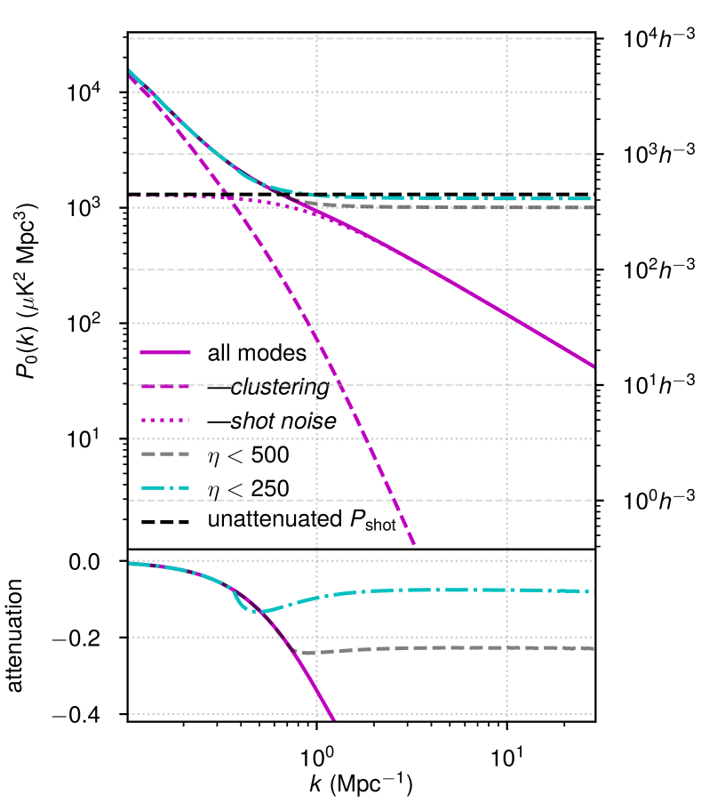
Figure 10: Illustration of the expected effect of line broadening on the total signal observed by mmIME at 100 GHz (indicated above each column of panels), with power spectra for all lines projected to the CO(3–2) frame at $z\sim 2.5$ and summed together. Upper panel: $P_{0}(k)$ calculated with the full formalism of Section 2 (magenta solid). For the full calculation we also show the clustering (magenta dashed) and shot-noise (magenta dotted) contributions separately. We also show the unattenuated total shot noise (black dashed), as well as the expected $P_{0}(k)$ when restricting calculations to modes with $\eta<500$ (grey dashed) or $\eta<250$ (cyan dash-dotted). Lower panel: Attenuation due to the introduction of line broadening, calculated using the full formalism (magenta solid). We again show the altered attenuation when restricting calculations to modes with $\eta<500$ (grey dashed) or $\eta<250$ (cyan dash-dotted).

6 Detailed Simulations

Returning to the context of COMAP and our fiducial model of CO(1–0) at $z\sim 3$, we find there is a need for explicit simulations of the CO intensity map across our fiducial distribution. The use of lightcones from a N-body cosmological simulation to generate these intensity maps mirrors the actual analysis expected for COMAP, and will also allow us to simulate the VID (with and without line broadening) without making the simplifying assumption of a log-normal galaxy count distribution as in Breysse et al. (2017).

6.1 Methods

The cosmological simulation used is the c400-2048 box from the Chinchilla suite. Li et al. (2016) used the same simulation and provide implementation details of the simulation and subsequent halo identification. The simulation spans $400h^{-1}$ Mpc on each side, and has a dark matter particle mass of $5.9\times 10^{8}h^{-1}\,M_{\odot}$. Since we only include the dark matter halo population with $M_{h}\geq 10^{10}\,M_{\odot}$ in our analysis, and although the box size is not quite large enough to encompass the full comoving line-of-sight span of the COMAP observation, we are mainly concerned with $k\gtrsim 0.1$ Mpc^-1 in this work. All in all, the size and resolution of this simulation should be sufficient for the purposes of this work.

We generate 100 lightcones spanning $z=1.5$–3.5 and a flat-sky area of $100^{\prime}\times 100^{\prime}$, each with its associated dark matter halo catalogue. As information relevant to the spatial orientation of the halo was not included at time of catalogue generation, we assign a random inclination angle $i$ to each halo. We then use limlam_mocker to assign a line luminosity to each halo according to the model outlined in Section 3.1. We generate 1280 CO(1–0) realizations, iterating through a random draw of 1280 samples of parameter values from our fiducial distribution, each assigned to one lightcone.

With the line luminosities fixed for each halo in each realization, we simulate a (noiseless) line-intensity cube spanning the full solid angle of the lightcone and 26–34 GHz in observing frequency (or $z=2.4$–3.4), with each voxel spanning $0.4^{\prime}\times 0.4^{\prime}\times 15.625$ MHz. For each realization, we generate cubes both with and without the COMAP beam of $4.5^{\prime}$ applied, and with the following five variations on simulating line broadening.

1. No line widths are specified—i.e., $v(M_{h})=0$ and thus $\sigma_{\parallel}(M_{h})=0$ for all $M_{h}$.

2. vmax64: Each halo has a calculated $v_{\text{max}}$, so we calculate the CO FWHM for each halo as $v_{\text{max}}\sin{i}/0.866$ and then bin the halo population by this FWHM in 64 linearly spaced bins. We generate a CO cube for each velocity bin separately, and apply a Gaussian filter to each cube along the line of sight, with the width of the Gaussian given by the median FWHM in each bin. We then sum the cubes across all bins to give the total CO temperature field. The maps generated using this approach serve as our ground truth for line broadening.

3. vvir64: We take the same approach as in vmax64 but using $v_{\text{vir}}(M_{h})$ instead of $v_{\text{max}}$, which (as previously discussed) peak-patch or other approximate N-body simulations may not provide.

4. veff: We apply a single Gaussian filter to the total CO temperature field along the line of sight, with the width of the Gaussian determined by $v_{\text{eff}}$ from Equation 46, calculated from the analytical halo model.

5. 2tier: This is the two-tier approach described in Section 4.2. We generate a CO cube from the $M_{h}<10^{11}\,M_{\odot}$ halo population with no line broadening, and bin the $M_{h}>10^{11}\,M_{\odot}$ population in 16 linearly spaced bins of $v_{\text{vir}}\sin{i}/0.866$. The appropriate Gaussian filter is applied along the line of sight to the CO cube for each FWHM bin, and we sum the CO cubes for all FWHM bins plus the $M_{h}<10^{11}\,M_{\odot}$ halo subset to give the total CO temperature field.

Whenever line broadening is applied, the CO cubes are initially generated with voxels that are four times finer in frequency space than the final voxels, so as to accurately model how the line intensity from each source is distributed across frequency channels. This combined with the Gaussian filter does increase the time required to compute the CO cube by almost a factor of 8, but as the calculation of various statistics of the cube takes significantly more time, there is not nearly as much impact on the time required to complete all calculations around each realization. Simulating line broadening across 16 bins (as in 2tier) or 64 bins (as in vmax64), this total time does increase approximately by factors of 3 to 10, but such overhead would be acceptable for COMAP analysis.

We calculate $P_{0}(k)$ for all cases. We also calculate $P_{2}(k)$ and the VID for all line broadening variations, but only when the COMAP beam is applied. For the VID, the CO cube is first coarsened to voxels of $4^{\prime}\times 4^{\prime}\times 15.625$ MHz to match the beam size, and then we calculate voxel counts $B_{i}$ across 75 log-spaced bins of $T_{i}\in(10^{0},10^{3})\,\mu$K. (Note that the mean temperature has been subtracted from the cube at this point.)

6.2 Results

Figure 11: Summary of simulated $z\sim 3$ CO(1–0) $P_{0}(k)$ across 1280 draws from our model posterior, using c400-2048 lightcones. We show medians and 90% intervals for each calculation, both ignoring angular resolution (left panels) and assuming smearing with a Gaussian beam of FWHM $4.5^{\prime}$ or $\sigma_{\perp}=3.5\text{\,Mpc}$ (right panels). Upper panels: $P_{0}(k)$ calculated without line broadening (yellow), using vmax64 (black) to calculate ground truth with line broadening, and three other variations: vvir64 (red), 2tier (cyan), and veff (magenta). Middle panels: Attenuation due to the introduction of line broadening, for each of the four variations prescribing non-zero line widths. Lower panels: Error from using vvir64, 2tier, or veff, relative to the ground truth (vmax64.

We show $P_{0}(k)$ from our simulations in Figure 11, both with and without beam smearing, and with all variations on line broadening. Note that the stalling of attenuation above $k\sim 1$ Mpc^-1 is an artefact of the limited line-of-sight resolution (we expect $k_{\parallel,\text{max}}\approx 0.9\text{\,Mpc}^{-1}$, corresponding to the 15.625 MHz voxel width).

Overall the results are not very surprising. Without beam smearing, all our approximations of line broadening perform very well, landing within several percent of ground truth (vmax64). while there is some breakdown with beam smearing introduced, it is confined to $k\gtrsim 0.5\text{\,Mpc}^{-1}$ where $P_{0}(k)$ is already significantly attenuated. The overall expected effect on a COMAP $P_{0}(k)$ detection is $\approx 7$% attenuation—consistent with the preliminary calculations from Section 5.2 using the representative parameters of Equations 27 through 31—with the 90% interval spanning 3% to 14% if we take possible variations in the $L(M_{h})$ model into account.

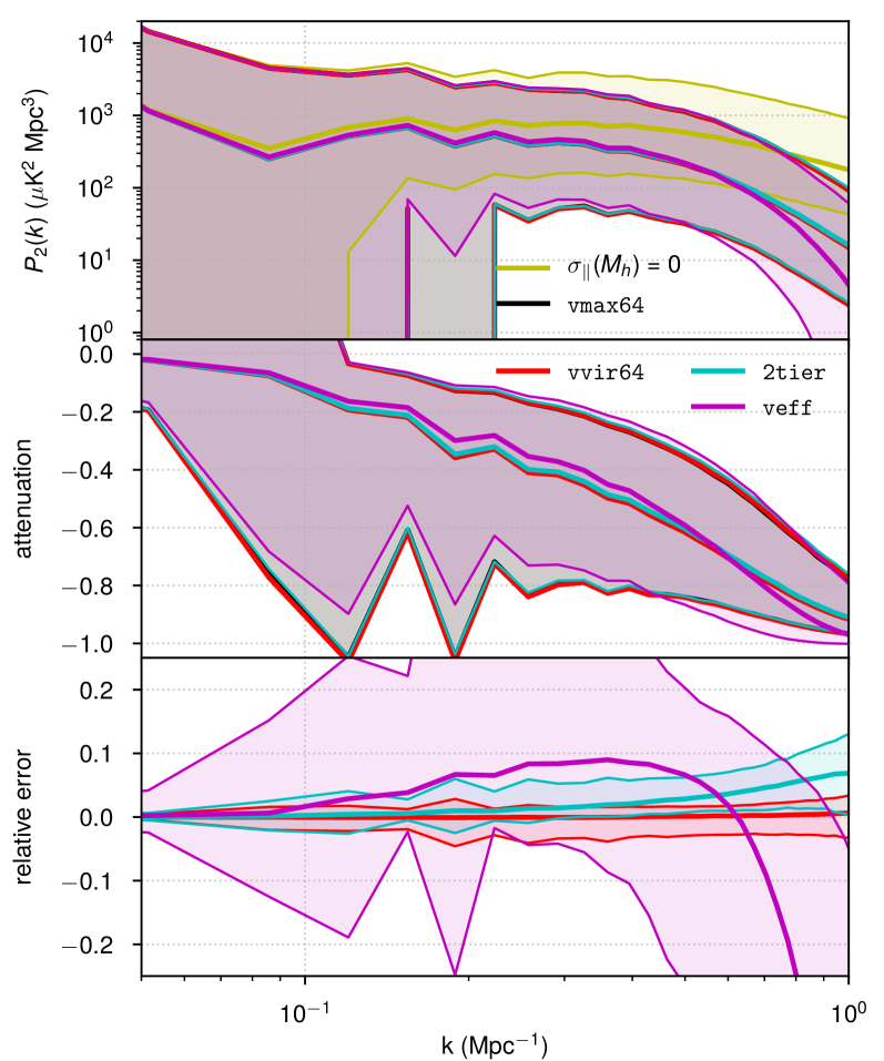
Figure 12: Similar to the right panels of Figure 11 (assuming smearing with a Gaussian beam of FWHM $4.5^{\prime}$ or $\sigma_{\perp}=3.5\text{\,Mpc}$), but summarising $P_{2}(k)$.

We also show $P_{2}(k)$ from our simulations (only in the presence of beam smearing) in Figure 12, although plotting only over a $k$-range of $(0.05,1)$ Mpc^-1 to redact both effects of finite box size and effects of limited spectral resolution in the simulated CO cube. The attenuation is much greater across $k$ than in $P_{0}(k)$, exceeding 30% by $k\sim 0.2$ Mpc^-1 in a majority of model draws. We also see that while the median relative error from ground truth is within 10% up to $k\sim 0.6$ Mpc^-1, the 90% interval in relative error from our allowed variations in $L(M_{h})$ can be much greater. The 2tier approach actually still results in acceptable accuracy here, even with the relatively low number of velocity bins. The distribution of relative error at higher $k$ values shows a negative skew, particularly for veff. This makes sense if we recall the discussion from Section 5.2. If the shot noise is much lower than the clustering component, using $v_{\text{eff}}$ will tend to over-attenuate, whereas the approximation will not tend to under-attenuate if the shot noise is dominant.

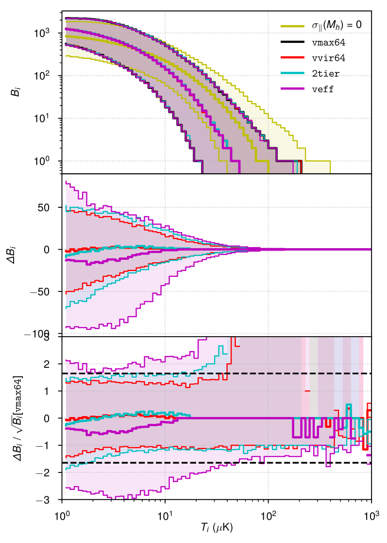
Figure 13: Summary of the simulated $z\sim 3$ CO(1–0) VID across 1280 draws from our model posterior, using c400-2048 lightcones. We show medians and 90% intervals for each calculation, both ignoring angular resolution (left panels) and assuming smearing with a Gaussian beam of FWHM $4.5^{\prime}$ or $\sigma_{\perp}=3.5\text{\,Mpc}$ (right panels). Upper panels: Bin counts $B_{i}$ calculated without line broadening (yellow), using vmax64 (black) to calculate ground truth with line broadening, and three other variations: vvir64 (red), 2tier (cyan), and veff (magenta). Middle panels: Absolute difference from ground truth (using vmax64) in $B_{i}$ for each of vvir64, 2tier, and veff. Lower panels: Difference from ground truth divided by the square root of the ground truth $B_{i}$, representing the relative difference in units of expected Poisson error. Black dashed lines at $\Delta B_{i}/\sqrt{B_{i}}=\pm 1.645$ represent the 90% interval expected with perfect Poisson errors across all bins.

Finally, in Figure 13 we consider the VID for the first time. Broadly, all line broadening simulation variations result in the same effect, shifting voxel counts from high $T_{i}$ to low $T_{i}$. But while the resulting $B_{i}$ are indistinguishable on a log-log plot, the deficiencies of the veff approach become clear when looking at a linear plot of the absolute error $\Delta B_{i}$ relative to ground truth. While using veff at least resulted in a reasonable estimate of $P_{2}(k)$ on average, here we see a clear systematic error at low $T_{i}$. When we consider $\Delta B_{i}/B_{i}^{1/2}$—that is, the ratio of this error to the Poisson error expected from the ‘true’ $B_{i}$—we find that veff is the only approach where the relative error from the approximation clearly in excess of Poisson error.

7 Discussion

7.1 The Inevitable Limitations of a Description of Line Broadening Using a Single Parameter

In the present state of line-intensity mapping, the primary observable for autocorrelation experiments similar to COMAP and mmIME remains the spherically-averaged monopole power spectrum $P_{0}(k)$, for which we have shown that the above $v_{\text{eff}}$ approximation works very well as a replacement for a numerically calculated transfer function for the shot-noise component. The results of the following subsection will also demonstrate that most of the time, this approximation allows us to match ground truth to within 10–20% at scales relevant to COMAP, a significant improvement over the systematic errors that would arise from neglecting line broadening. Therefore, for forecasting or analysis of the line-intensity $P_{0}(k)$, using a single $v_{\text{eff}}$ is adequate.

However, clear shortcomings to this approach exist. One shortcoming, which is perhaps not overly relevant in application to analysis, is that the approximation breaks down at sufficiently high $k$ in the presence of an angular beam of sufficiently large comoving size. In the case of COMAP, an angular size of 4.5 arcminutes on sky corresponds to $\sigma_{\perp}\approx 3.5$ Mpc at the central COMAP redshift, compared to typical values of $\sigma_{\parallel,\text{eff}}\sim 1.5$–2 Mpc that we would expect from $v_{\text{eff}}\approx 250$–350 km s^-1. Yet we have not accounted for the angular beam in our approximation above.

We might contemplate accounting for $\sigma_{\perp}$ explicitly, via appropriately tweaking Equation 42. However, calculations in LABEL:sec:madansatz show that doing so does not actually improve relative error in any appreciable fashion. The fundamental truth is that we fully expect these kinds of approximations to fail at sufficiently high $k$. We note that, looking at the lower right panel of Figure 11 for the median relative error in $P_{0}(k)$ versus ground truth when using $v_{\text{eff}}$, this relative error only exceeds 10% for $k\gtrsim 0.9\text{\,Mpc}^{-1}\approx\pi/\sigma_{\perp}$. So in practice, this concern at least should not be too relevant to analysis, where the $P_{0}(k)$ loss around this $k$-range is already sufficiently high ($\gtrsim 80$%) that data here are likely to be discarded.

However, our approximation remains wanting in analysis due to concerns that are extremely relevant in the context of analyses like Ihle et al. (2019) that deal with the VID rather than just $P(k)$. The central motivation behind using the VID jointly with $P(k)$, as explained in previous works like Breysse et al. (2017), is that the CO intensity field observed by COMAP is highly non-Gaussian, so that the VID contains substantial information beyond $P(k)$. Just as $P(k)$ therefore does not fully determine the VID, the $P_{0}(k)$ transfer function does not fully determine the VID transfer function. Therefore, a single parameter describing the $P_{0}(k)$ transfer function from line broadening—which summarizes our approach with a single $v_{\text{eff}}$—would never be able to fully describe the effect of line broadening on the VID.

Even without thinking about non-Gaussianities explicitly, we can consider an extreme scenario. Suppose we have 1000 emitters with 999 of them at $L\sim 10^{4}\,L_{\odot}$ and negligible line broadening, and only one at $L\sim 10^{6}\,L_{\odot}$ but line width of $v\sim 300$ km s^-1, so that

$$\frac{dn}{dL}\propto 999\delta_{D}(L-10^{4}\,L_{\odot})+\delta_{D}(L-10^{6}\,L_{\odot}),$$ (53)

where we use $\delta_{D}$ to denote the (one-dimensional) Dirac delta function. Given this $dn/dL$, clearly the fainter but more numerous emitters dominate the clustering component and occupy the overwhelming majority of voxels, but the single bright emitter will dominate any $L^{2}$-weighted statistics by itself, including shot noise and our effective line width:

$$v_{\text{eff}} =\frac{\int dL\,\frac{dn}{dL}\,L^{2}v(L)}{2\int dL\,\frac{dn}{dL}\,L^{2}}+\frac{\int dL\,\frac{dn}{dL}\,L^{2}}{2\int dL\,\frac{dn}{dL}\,L^{2}/v(L)}$$ (54)

$$=\frac{(10^{6}\,L_{\odot})^{2}\cdot 300\text{\,km\,s}^{-1}}{999\cdot(10^{4}\,L_{\odot})^{2}+(10^{6}\,L_{\odot})^{2}}\approx 270\text{\,km\,s}^{-1}{.}$$ (55)

So if we use a single Gaussian filter across the entire CO cube as in the previous subsection’s treatment, then we will broaden all line profiles by almost the full line width of the single bright emitter. This may not affect $P_{0}(k)$ too much—the full 3D $P(\mathbf{k})$ may be somewhat affected but the effect on the averaged $P_{0}(k)$ will be small at smaller scales (where the bright emitter dominates the shot noise power spectrum anyway) and even less at larger scales. However, this $v_{\text{eff}}$ prescription will distort the VID significantly, as we see in Figure 13. Voxels around the locations of fainter emitters, which should be in low-temperature bins of $T_{i}\sim 10^{0}$–$10^{1}\,\mu\text{K}$ in a proper simulation, instead end up with overly low temperatures of $\lesssim 10^{0}\,\mu\text{K}$ due to excessive line broadening. No procedure can avoid this effect if it will apply the same line width to a halo subset spanning orders of magnitude in various properties, which is to say that a very coarse binning of the halo catalogue in a simulation into two or three subsets is unlikely to substantially correct for VID distortion.

In summary, for any analyses that involve $P_{0}(k)$ detection by itself, our $v_{\text{eff}}$ prescription is valid. But we need a more thorough line broadening simulation procedure for anything more advanced—not just the VID, but other statistics like higher-order moments of the full 3D power spectrum that we could consider as part of future COMAP science. What distinguishes line-intensity mapping from line candidate scans or targeted galaxy surveys is the measurement of aggregate line emission from both bright and faint galaxies. We therefore neglect faint line emitters at our own peril, not only in models of the signal but also in models of systematic effects.

7.2 Challenges for Interpretation of Single-dish and Interferometric LIM Surveys

Qualitatively, line broadening poses the same challenges for single-dish surveys like COMAP as for interferometric surveys like COPSS and mmIME. The primary challenge is the attenuation of the power spectrum to begin with, which somewhat raises sensitivity requirements to achieve a given signal-to-noise ratio for $P(k)$. The secondary challenge—just as important—is in interpretation of a detection, which requires accurate correction for the attenuation.

The work here lets us gauge the former, but not necessarily the latter. We have seen above that, in the context of an initial detection with a signal-to-noise ratio of 3–5, the attenuation of the power spectrum due to line broadening would be small or can be reduced with appropriate redaction of the data to a level that is subdominant to uncertainties from noise. However, once LIM surveys reach higher detection significance, we will no longer be able to ignore either this correction or the uncertainties around the various assumptions around line profile width and shape that underlie the correction.

Quantitatively, speaking very specifically about the problem of line broadening as it relates to detection of $P_{0}(k)$, single-dish surveys are at an advantage over interferometric surveys. The attenuation expected for COMAP at $k\sim 0.2$–0.3 Mpc^-1 is around 10%, whereas for mmIME the attenuation expected at $k\sim 10$ Mpc^-1 is around 25% even with the calculations restricted to $\eta<500$ (which discards modes above a certain $k_{\parallel}$ and thus is part of a sensitivity trade-off between number of Fourier modes and signal recovery). This means COMAP requires only a 11% correction, versus 33% for mmIME. If model uncertainties add relative error to this correction, interferometric surveys have the larger correction to begin with and thus will bear more of a challenge.

This, however, is only part of the story. If COMAP analyses make use of statistics that put more weight on small-scale data, such as the quadrupole $P_{2}(k)$ (with its shot-noise component from anisotropic smearing) or the VID, these analyses will rely heavily on models of line broadening. Even without undertaking rigorous simulations, we can consider a more extreme scenario where the true line profile is described by either a top-hat profile or a Gaussian profile. These two shapes are clearly going to result in very different kernels for the VID, and if the two are equally likely then we will need to split the difference and indicate appropriate uncertainties.

In the case of high-redshift CO, we think the Gaussian assumption is well-justified as it has served well in the context of untargeted high-redshift CO line searches like ASPECS, where the Gaussian shape is a reasonable fit for most (although not all) of the detections by González-López et al. (2019). However, if we did want to seriously consider other possible line shapes like double-Gaussian or double-horned profiles, we must account in inferences for the uncertainty from such variations. We leave this problem to future work.

8 Conclusions

The scope of this work, simply put, was to answer three questions posited in the Introduction. As we conclude, we find an answer to each question (partly reproduced):

1. What is the level of signal attenuation that we can expect for experiments like COMAP and mmIME due to line broadening? Our median expectation for COMAP is a $\lesssim 10\%$ attenuation of the line-intensity $P_{0}(k)$ at relevant scales, with the 90% interval from our fiducial model ensemble being 3–14%. Our prediction of the effect for mmIME is larger, broadly agreeing with the expectation of Keating et al. (2020) of 25% attenuation after data cuts.

2. Is it sufficient to describe the effect of line broadening using a single parameter, such as an effective global line width? We have described a way to calculate an effective global line width that does, in fact, allow for a reasonable approximation of the effect of line broadening on the monopole $P_{0}(k)$.

3. How does this simplification fail? The approximation has greater errors for the quadrupole $P_{2}(k)$, and results in significant systematic error in the context of the VID. These results demonstrate the overdetermined nature of attempting to define a single effective global line width to describe non-Gaussian statistics.

The effect of line broadening is thus less critical for initial upper limits or detections (where uncertainties from noise will likely dominate over any uncertainty in corrections for line broadening), but has serious implications for more advanced analyses hoping to make use of other statistics like $P_{2}(k)$ or the VID. The strong attenuation of $P_{2}(k)$ may have non-negligible effects on the signal-to-noise required for cosmological analyses of the kind proposed by Bernal et al. (2019a, b). Although the challenge is not insurmountable in theory, it will necessitate building more sensitive instruments or operating longer surveys than we may have previously thought.

We make no claim that our $v(M_{h})$ model for CO(1–0) at $z\sim 3$ is entirely accurate, but it is consistent with the information we have at the time of writing. It is however somewhat tenuous as tying the line width directly to the halo circular velocity carries assumptions about gas density profiles and dynamics that we discussed briefly in Section 3.2. Any future work that directly contradicts these assumptions would automatically demand revisions of our model.

It will be important going forward to study in great detail the line profile shape and width of both faint and bright high-redshift galaxies in various lines, and how these correlate with properties that we may be able to connect to halo properties in dark matter simulations. This will be particularly important in studying the luminosity function and non-Gaussianities via the VID, where the line shape may perhaps be even more important than the width.

Paradoxically it may be line-intensity mapping that may be best suited to study some of these properties in certain regimes. If we find, for instance, that LIM observables like $P_{\ell}(k)$ and the VID are not well described using models of line broadening devised with data from untargeted line searches like ASPECS, then it may indicate something about the line profiles of faint emitters that differs from the line profiles of bright emitters as studied by line searches (or at least the extrapolation from bright emitters to faint emitters that would have been used).

Overall, line broadening is a systematic obstacle to detection and interpretation of LIM signals, but by no means a catastrophic one. We trust that future work—not only in simulation but also in observation—will continue to shed light on the problem and offer fresh approaches.

Appendix A Explicit Analytic Corrections for Inclination

Under the specific but reasonable assumption of randomly oriented, rotation-dominated emitters, we may introduce an analytic correction to the expressions of Section 2. Instead of $\sigma_{v}(M_{h})$, the applicable width is $\sigma_{v}$ times a random $\sin{i}$—or rather $\sin{i}/0.866$, if we assume that the mean $\sigma_{v}$ value corresponds to the median value of $\sin{i}=\sqrt{3}/2$. For random orientation, the distribution of $\cos{i}$ is uniform such that the average attenuation of the shot noise at fixed $k$ and $\mu$ may be calculated as follows (partly via Mathematica):

$$P_{\text{shot,v},i}(k,\mu) =C_{LT}^{2}\int dM_{h}\int_{0}^{1}d{(\cos{i})}\,\frac{dn}{dM_{h}}\,L^{2}(M_{h})\exp{\left[-k^{2}\sigma_{\perp}^{2}(1-\mu^{2})-k^{2}\sigma_{v}^{2}(M_{h})\mu^{2}\cdot\frac{1-\cos^{2}{i}}{3/4}\right]}$$

$$=C_{LT}^{2}\int dM_{h}\,\frac{dn}{dM_{h}}\,L^{2}(M_{h})\exp{\left[-k^{2}\sigma_{\perp}^{2}(1-\mu^{2})\right]}\left[\frac{2k\sigma_{v}(M_{h})\mu}{\sqrt{3}}\right]^{-1}F{\left(\frac{2k\sigma_{v}(M_{h})\mu}{\sqrt{3}}\right)},$$ (A1)

where $F(x)$ is Dawson’s integral. (For our purposes, we consider $F(x)/x$ to evaluate to $1$ at $x=0$.) With similar replacements, we can calculate the clustering component as follows:

$$P_{\text{clust},v,i}(k,\mu) =C_{LT}^{2}P_{m}(k)\left\{\int dM_{h}\,\frac{dn}{dM_{h}}\,L(M_{h})\left[b(M_{h})+\Omega_{m}(z)^{0.55}\mu^{2}\right]\times\right.$$

$$\qquad\left.\exp{\left[-\frac{k^{2}\sigma_{\perp}^{2}(1-\mu^{2})}{2}\right]}\left[\frac{\sqrt{2}k\sigma_{v}(M_{h})\mu}{\sqrt{3}}\right]^{-1}F{\left(\frac{\sqrt{2}k\sigma_{v}(M_{h})\mu}{\sqrt{3}}\right)}\right\}^{2}.$$ (A2)

We have inadvertently assumed that perfectly face-on galaxies will have an observed line FWHM of zero, which cannot possibly true for several reasons. The foremost astrophysical reason is that the CO gas will have its own velocity dispersion independent of the overall rotation. For instance, de Blok & Walter (2014) consider dispersions of 10 or 50 km s^-1 for low- and high-redshift galaxies. Furthermore, finite frequency resolution means we would never observe even point sources as point sources. Gas dispersions of 10–50 km s^-1 are certainly subdominant to the $\approx 16$ MHz channelization used both in this work in Section 6 and in Keating et al. (2020) for mmIME data. On a more pragmatic level, the randomly drawn inclinations will rarely hit very close to face-on, and certainly never exactly face-on—less than 0.5% of simulated emitters would have $\sin{i}<0.1$—so we believe this oversight may be overlooked.

We can get an approximate idea of the level of correction this introduces for the shot noise by calculating the ratio of the integrands in Equation 13 and Equation A1. For $k\sigma_{v}\mu\sim 0.1$ the ratio is within a few percent of unity, but for $k\sigma_{v}\mu\gtrsim 1$ the relative difference begins to exceed 10%. Therefore, as the effect is greater at smaller scales, it will clearly affect simulations of the VID.

We turn to implications for our effective line widths. The main task is to adjust our high-$k$ ansatz, as the smaller scales are most affected. The integral of Equation A1 in $\mu\in(0,1)$ (setting $\sigma_{\perp}=0$) is unfortunately somewhat less pleasant than before:

$$P_{0,\text{shot},v,i}=C_{LT}^{2}\left\langle{L^{2}\,{}_{2}F_{2}\left(\frac{1}{2},1;\frac{3}{2},\frac{3}{2};-\frac{4k^{2}\sigma_{v}^{2}}{3}\right)}\right\rangle,$$ (A3)

where ${}_{2}F_{2}$ denotes the generalized hypergeometric function. Looking at $k\sigma_{v}\to\infty$, the leading-order behaviour is such that

$${}_{2}F_{2}\left(\frac{1}{2},1;\frac{3}{2},\frac{3}{2};-\frac{4k^{2}\sigma_{v}^{2}}{3}\right)\sim\frac{\pi^{3/2}}{4}\left(\frac{2}{\sqrt{3}}k\sigma_{v}\right)^{-1}.$$ (A4)

Compare to Equation 40 and Equation 41, where the prefactor for $\operatorname{erf}{(k\sigma)}/(k\sigma)\sim(k\sigma)^{-1}$ is $\pi^{1/2}/2$. Thus we should multiply the high-$k$ ansatz by the ratio of the two prefactors, which is $4/(\pi\sqrt{3})\approx 0.735$. (Note that if we were assuming $\sigma_{v}(M_{h})$ were the value for face-on galaxies as opposed to $\cos{i}=0.5$, the correction would be greater, requiring multiplication by $2/\pi\approx 0.637$.) Thus we derive the inclination-corrected $v_{\text{eff}}$ of Equation 46 as the midpoint between the inclination-corrected high-$k$ ansatz and $\left\langle{L^{2}v}\right\rangle/\left\langle{L^{2}}\right\rangle$ as is, as the latter approximates the line broadening effect at values of $k$ where incorporating inclination does not yield appreciable changes.

Appendix B Approximate Analytic Validation of Effective Line Width Ansatz

An exact analytic validation of our ansatz for the effective line width is challenging on multiple levels. The error function is a decidedly non-elementary function, and $dn/dM_{h}$ also takes a somewhat complex form, specified for instance by Murray et al. (2018) by a generalized Schechter function (i.e., a power law with exponential cutoff of variable sharpness). We can however show for a highly simplified model that it really is a reasonable ansatz through a basic polynomial approximation to the error function.

As the model of Murray et al. (2018) suggests, $dn/dM_{h}\sim M_{h}^{-2}$ up to the exponential cutoff, although some variation in this power-law slope exists. Here we simplify the picture drastically so that $dn/dM_{h}$ is such a power law up to some maximum $M$ and equal to zero above it. If we suppose $L(M_{h})$ follows a power law up to that cutoff, we broadly expect that power-law slope to be at least positive if not super-linear. We could leave $v(M)$ as a generic power law leaving the slope unspecified, but for illustrative purposes and given physical expectations, we will fix $v(M)\sim M^{1/3}$.

Up to various constants and coefficients that we will omit, our ansatz is

$$\frac{\left\langle{L^{2}v}\right\rangle}{\left\langle{L^{2}}\right\rangle}+\frac{\left\langle{L^{2}}\right\rangle}{\left\langle{L^{2}v^{-1}}\right\rangle} =\frac{1}{2}\left(\frac{\int dM_{h}\,M_{h}^{a+1/3}}{\int dM_{h}\,M_{h}^{a}}+\frac{\int dM_{h}\,M_{h}^{a}}{\int dM_{h}\,M_{h}^{a-1/3}}\right)$$

$$=\frac{M^{1/3}}{2}\left(\frac{a+1}{a+4/3}+\frac{a+2/3}{a+1}\right).$$ (B1)

Now we consider solving for $\sigma_{\parallel}$ in Equation 42 using different approximations in different regimes. We will however replace $k\sigma_{\parallel,\text{eff}}$ with $M_{\text{eff}}^{1/3}$ and $k\sigma_{\parallel}(M_{h})$ with $M_{h}^{1/3}$ to simplify our calculations. It will not affect our conclusions around the relative error of different approximations in different regimes.

We can broadly think of three different regimes: $k\sigma\ll 1$, $k\sigma\lesssim 1$, and $k\sigma\gg 1$. In the first regime of very large scales and/or very small masses or velocities, attenuation is minimal and Equation 42 is almost tautological. In the last regime of very small scales and/or very large masses or velocities, $\operatorname{erf}{(x)}/x\approx 1/x$ and so we actually approach the second component of our ansatz, $\left\langle{L^{2}}\right\rangle/\left\langle{L^{2}v^{-1}}\right\rangle$.

In the middle regime, we use a second-order Taylor series approximation: $\operatorname{erf}(x)/x\approx 2\pi^{-1/2}(1-x^{2}/3)$ (within 5% up to $x=0.8$). Since the prefactor will cancel anyway when calculating $M_{\text{eff}}$, we consider the $L^{2}$-weighted average $1-M_{h}^{2/3}/3$:

$$1-\frac{M_{\text{eff}}^{2/3}}{3}=\frac{\int dM_{h}\,M_{h}^{a}(1-M_{h}^{2/3}/3)}{\int dM_{h}\,M_{h}^{a}}=1-\frac{a+1}{3a+5}M^{2/3},$$ (B2)

which is to say that

$$M_{\text{eff}}^{1/3}=\left(\frac{a+1}{a+5/3}\right)^{1/2}M^{1/3}.$$ (B3)

So now we can compare the coefficients in front of $M^{1/3}$ for each approximation—the $\left\langle{L^{2}v}\right\rangle/\left\langle{L^{2}}\right\rangle$ ansatz; the $\left\langle{L^{2}}\right\rangle/\left\langle{L^{2}v^{-1}}\right\rangle$ ansatz which the truth will approach as $k\sigma\to\infty$; the $k\sigma\lesssim 1$ approximation; and the midpoint ansatz:

$$C_{v} =\frac{a+1}{a+4/3}$$ (B4)

$$C_{v^{-1}} =\frac{a+2/3}{a+1}$$ (B5)

$$C_{k\sigma\lesssim 1} =\left(\frac{a+1}{a+5/3}\right)^{1/2}$$ (B6)

$$C_{\text{eff}} =\frac{C_{v}+C_{v^{-1}}}{2}=\frac{1}{2}\left(\frac{a+1}{a+4/3}+\frac{a+2/3}{a+1}\right)$$ (B7)

If $dn/dM_{h}\sim M_{h}^{-2}$, then $a=0$ would correspond to a roughly linear $L(M_{h})$, and values above this to models with super-linear $L(M_{h})$ like our fiducial model ultimately is at low mass. Therefore we can heuristically consider how our different approximations compare for different faint-end $L(M_{h})$ slopes.

It is clear by inspection that $C_{v}>C_{v^{-1}}$ and that for high $a$ (i.e., for a sufficiently steep $L(M_{h})$ power law) these approximations become more similar. The latter point is not necessarily worth much thought when we return to more realistic models, as the approximations may still diverge depending on the model behaviour at high mass (where we have not specified the exponential cutoff and bright-end power law at all). Even with the former point, we do note that for values of $a$ around 2 or 3 (which we might expect for $dn/dM_{h}\sim M^{-2}$ and a faint-end $L(M)\sim M_{h}^{2}$ or $M_{h}^{2.5}$), the difference is not too great at around 10%. So while $C_{v}$ clearly differs from $C_{v^{-1}}$ it is still surprisingly close for a blind guess.

Perhaps even more surprising is the closeness between $C_{v}$ and $C_{k\sigma\lesssim 1}$, the latter being the best we can do analytically within reason at intermediate scales. It is perhaps clearer if we explicitly express the ratio between the two,

$$\frac{C_{v}}{C_{k\sigma\lesssim 1}}=\frac{[(a+1)(a+5/3)]^{1/2}}{a+4/3}.$$ (B8)

We note first that the ratio is quite close to unity—$C_{v}$ is within 5% of $C_{k\sigma\lesssim 1}$ for values of $a$ around 2 or 3. But we also note that this ratio is one between an arithmetic mean and a geometric mean. Since the arithmetic mean of two non-negative real numbers is always greater than their geometric mean, it is always true that $C_{v}<C_{k\sigma\lesssim 1}$ (as long as a real value of $C_{k\sigma\lesssim 1}$ exists for comparison).

We thus have $C_{v^{-1}}<C_{v}<C_{k\sigma\lesssim 1}$, with $C_{v}$ being close to truth at intermediate scales and $C_{v^{-1}}$ being close to truth at $k\sigma\gg 1$ but necessarily further away from truth at intermediate scales compared to $C_{v}$. The midpoint ansatz represented by $C_{\text{eff}}$ is a clear compromise—not the optimal choice in any single regime but able to reduce the maximum error across all regimes.

Appendix C Projection of mmIME Power Spectra

We refer to Lidz & Taylor (2016) for the calculations required to project each of the power spectra in Figure 9 to a common frame—namely the $z\sim 2.5$ frame applicable for CO(3–2)—and sum these together for the result shown in Figure 10.

To map the wavevector $\mathbf{k}_{J}$ for the CO($J\to J-1$) line at redshift $z_{J}$ to the apparent wavevector $\mathbf{k}$ in the CO(3–2) frame at redshift $z=z_{J=3}$, we need only consider how the parallel and perpendicular components $k_{\perp,J}$ and $k_{\parallel,J}$ map to $k_{\perp}$ and $k_{\parallel}$ in the CO(3–2) frame. Equations 5 and 6 of Lidz & Taylor (2016) give these mappings (notation altered to match our own):

$$k_{\parallel}=\underbrace{\frac{H(z)}{H(z_{J})}\frac{1+z_{J}}{1+z}}_{\alpha_{\parallel,J}}k_{\parallel,J};\qquad k_{\perp}=\underbrace{\frac{R(z_{J})}{R(z)}}_{\alpha_{\perp,J}}k_{\perp,J}.$$ (C1)

Here we have used our assumption of a flat universe to replace the comoving angular diameter distance used in Equation 6 of Lidz & Taylor (2016) with simply the comoving distance $R(z)$.

Then Equation 7 of Lidz & Taylor (2016) gives the anisotropic power spectrum as a function of $k_{\parallel}$ and $k_{\perp}$, so that we can describe the sum of the anisotropic power spectra in the common CO(3–2) frame,

$$P_{\text{tot}}(k_{\parallel},k_{\perp})=\sum_{J}\frac{P_{J}(k_{\parallel}/\alpha_{\parallel,J},k_{\perp}/\alpha_{\perp,J})}{\alpha_{\parallel,J}\alpha_{\perp,J}^{2}}.$$ (C2)

In this work, we have always dealt with power spectra as functions of $k$ and $\mu$. Recall that $\mu$ is the dot product between $\hat{\mathbf{k}}$ and the line-of-sight unit vector, so that

$$k_{\parallel}=k\mu;\qquad k_{\perp}=k(1-\mu^{2})^{1/2}.$$ (C3)

Then we can map the apparent $k$ and $\mu$ in the CO(3–2) frame to the true $k_{J}$ and $\mu_{J}$ corresponding to the arguments to $P_{J}$ in Equation C2:

$$k_{J}=k\left(\frac{\mu^{2}}{\alpha_{\parallel,J}^{2}}+\frac{1-\mu^{2}}{\alpha_{\perp,J}^{2}}\right)^{1/2};\qquad\mu_{J}=\frac{k\mu}{\alpha_{\parallel,J}k_{J}}.$$ (C4)

So given the above relations, we can write

$$P_{\text{tot}}(k,\mu)=\sum_{J}\frac{P_{J}[k_{J}(k,\mu),\mu_{J}(k,\mu)]}{\alpha_{\parallel,J}\alpha_{\perp,J}^{2}}.$$ (C5)

We use this rewritten expression to sum the anisotropic power spectra for $J=2$ through $J=5$ in the main text and thus evaluate the total $P_{0}(k)$ in the CO(3–2) frame as shown in Figure 10.

References

- Aravena et al. (2019) Aravena, M., Decarli, R., Gónzalez-López, J., et al. 2019, ApJ, 882, 136, doi: 10.3847/1538-4357/ab30df
- Astropy Collaboration et al. (2013) Astropy Collaboration, Robitaille, T. P., Tollerud, E. J., et al. 2013, A&A, 558, A33, doi: 10.1051/0004-6361/201322068
- Behroozi et al. (2019) Behroozi, P., Wechsler, R. H., Hearin, A. P., & Conroy, C. 2019, MNRAS, 488, 3143, doi: 10.1093/mnras/stz1182
- Behroozi et al. (2013a) Behroozi, P. S., Wechsler, R. H., & Conroy, C. 2013a, ApJ, 762, L31, doi: 10.1088/2041-8205/762/2/L31
- Behroozi et al. (2013b) —. 2013b, ApJ, 770, 57, doi: 10.1088/0004-637X/770/1/57
- Bernal et al. (2019a) Bernal, J. L., Breysse, P. C., Gil-Marín, H., & Kovetz, E. D. 2019a, Phys. Rev. D, 100, 123522, doi: 10.1103/PhysRevD.100.123522
- Bernal et al. (2019b) Bernal, J. L., Breysse, P. C., & Kovetz, E. D. 2019b, Phys. Rev. Lett., 123, 251301, doi: 10.1103/PhysRevLett.123.251301
- Breysse & Alexandroff (2019) Breysse, P. C., & Alexandroff, R. M. 2019, MNRAS, 490, 260, doi: 10.1093/mnras/stz2534
- Breysse et al. (2017) Breysse, P. C., Kovetz, E. D., Behroozi, P. S., Dai, L., & Kamionkowski, M. 2017, MNRAS, 467, 2996, doi: 10.1093/mnras/stx203
- Bryan & Norman (1998) Bryan, G. L., & Norman, M. L. 1998, ApJ, 495, 80, doi: 10.1086/305262
- Capak et al. (2015) Capak, P. L., Carilli, C., Jones, G., et al. 2015, Nature, 522, 455, doi: 10.1038/nature14500
- Chang et al. (2008) Chang, T.-C., Pen, U.-L., Peterson, J. B., & McDonald, P. 2008, Phys. Rev. Lett., 100, 091303, doi: 10.1103/PhysRevLett.100.091303
- Chung (2019) Chung, D. T. 2019, ApJ, 881, 149, doi: 10.3847/1538-4357/ab3040
- Chung et al. (2020) Chung, D. T., Viero, M. P., Church, S. E., & Wechsler, R. H. 2020, ApJ, 892, 51, doi: 10.3847/1538-4357/ab798f
- Concerto Collaboration et al. (2020) Concerto Collaboration, Ade, P., Aravena, M., et al. 2020, A&A, 642, A60, doi: 10.1051/0004-6361/202038456
- Cothard et al. (2020) Cothard, N. F., Choi, S. K., Duell, C. J., et al. 2020, Journal of Low Temperature Physics, 199, 898, doi: 10.1007/s10909-019-02297-1
- Daddi et al. (2015) Daddi, E., Dannerbauer, H., Liu, D., et al. 2015, A&A, 577, A46, doi: 10.1051/0004-6361/201425043
- de Blok & Walter (2014) de Blok, W. J. G., & Walter, F. 2014, AJ, 147, 96, doi: 10.1088/0004-6256/147/5/96
- Dumitru et al. (2019) Dumitru, S., Kulkarni, G., Lagache, G., & Haehnelt, M. G. 2019, MNRAS, 485, 3486, doi: 10.1093/mnras/stz617
- Faber & Jackson (1976) Faber, S. M., & Jackson, R. E. 1976, ApJ, 204, 668, doi: 10.1086/154215
- Foreman-Mackey et al. (2013) Foreman-Mackey, D., Hogg, D. W., Lang, D., & Goodman, J. 2013, PASP, 125, 306, doi: 10.1086/670067
- Freundlich et al. (2019) Freundlich, J., Combes, F., Tacconi, L. J., et al. 2019, A&A, 622, A105, doi: 10.1051/0004-6361/201732223
- González-López et al. (2019) González-López, J., Decarli, R., Pavesi, R., et al. 2019, ApJ, 882, 139, doi: 10.3847/1538-4357/ab3105
- Goto & Toft (2015) Goto, T., & Toft, S. 2015, A&A, 579, A17, doi: 10.1051/0004-6361/201526062
- Harris et al. (2012) Harris, A. I., Baker, A. J., Frayer, D. T., et al. 2012, ApJ, 752, 152, doi: 10.1088/0004-637X/752/2/152
- Hinshaw et al. (2013) Hinshaw, G., Larson, D., Komatsu, E., et al. 2013, ApJS, 208, 19, doi: 10.1088/0067-0049/208/2/19
- Hunter (2007) Hunter, J. D. 2007, Computing In Science & Engineering, 9, 90, doi: 10.1109/MCSE.2007.55
- Ihle et al. (2019) Ihle, H. T., Chung, D., Stein, G., et al. 2019, ApJ, 871, 75, doi: 10.3847/1538-4357/aaf4bc
- Kamenetzky et al. (2016) Kamenetzky, J., Rangwala, N., Glenn, J., Maloney, P. R., & Conley, A. 2016, ApJ, 829, 93, doi: 10.3847/0004-637X/829/2/93
- Keating et al. (2020) Keating, G. K., Marrone, D. P., Bower, G. C., & Keenan, R. P. 2020, ApJ, 901, 141, doi: 10.3847/1538-4357/abb08e
- Keating et al. (2016) Keating, G. K., Marrone, D. P., Bower, G. C., et al. 2016, ApJ, 830, 34, doi: 10.3847/0004-637X/830/1/34
- Klypin et al. (2016) Klypin, A., Yepes, G., Gottlöber, S., Prada, F., & Heß, S. 2016, MNRAS, 457, 4340, doi: 10.1093/mnras/stw248
- Kovetz et al. (2019) Kovetz, E., Breysse, P. C., Lidz, A., et al. 2019, BAAS, 51, 101. https://arxiv.org/abs/1903.04496
- Kovetz et al. (2017) Kovetz, E. D., Viero, M. P., Lidz, A., et al. 2017, arXiv e-prints, arXiv:1709.09066. https://arxiv.org/abs/1709.09066
- Li et al. (2016) Li, T. Y., Wechsler, R. H., Devaraj, K., & Church, S. E. 2016, ApJ, 817, 169, doi: 10.3847/0004-637X/817/2/169
- Lidz et al. (2011) Lidz, A., Furlanetto, S. R., Oh, S. P., et al. 2011, ApJ, 741, 70, doi: 10.1088/0004-637X/741/2/70
- Lidz & Taylor (2016) Lidz, A., & Taylor, J. 2016, ApJ, 825, 143, doi: 10.3847/0004-637X/825/2/143
- Madau et al. (1997) Madau, P., Meiksin, A., & Rees, M. J. 1997, ApJ, 475, 429, doi: 10.1086/303549
- Mashian et al. (2015) Mashian, N., Sternberg, A., & Loeb, A. 2015, J. Cosmology Astropart. Phys, 2015, 028, doi: 10.1088/1475-7516/2015/11/028
- Moradinezhad Dizgah & Keating (2019) Moradinezhad Dizgah, A., & Keating, G. K. 2019, ApJ, 872, 126, doi: 10.3847/1538-4357/aafd36
- Murray et al. (2013) Murray, S. G., Power, C., & Robotham, A. S. G. 2013, Astronomy and Computing, 3, 23, doi: 10.1016/j.ascom.2013.11.001
- Murray et al. (2018) Murray, S. G., Robotham, A. S. G., & Power, C. 2018, ApJ, 855, 5, doi: 10.3847/1538-4357/aaa552
- Newman et al. (2013) Newman, S. F., Genzel, R., Förster Schreiber, N. M., et al. 2013, ApJ, 767, 104, doi: 10.1088/0004-637X/767/2/104
- Padmanabhan (2018) Padmanabhan, H. 2018, MNRAS, 475, 1477, doi: 10.1093/mnras/stx3250
- Padmanabhan (2019) —. 2019, MNRAS, 488, 3014, doi: 10.1093/mnras/stz1878
- Pavesi et al. (2018) Pavesi, R., Sharon, C. E., Riechers, D. A., et al. 2018, ApJ, 864, 49, doi: 10.3847/1538-4357/aacb79
- Pentericci et al. (2016) Pentericci, L., Carniani, S., Castellano, M., et al. 2016, ApJ, 829, L11, doi: 10.3847/2041-8205/829/1/L11
- Planck Collaboration XIII (2016) Planck Collaboration XIII. 2016, A&A, 594, A13, doi: 10.1051/0004-6361/201525830
- Pullen et al. (2013) Pullen, A. R., Chang, T.-C., Doré, O., & Lidz, A. 2013, ApJ, 768, 15, doi: 10.1088/0004-637X/768/1/15
- Riechers et al. (2019) Riechers, D. A., Pavesi, R., Sharon, C. E., et al. 2019, ApJ, 872, 7, doi: 10.3847/1538-4357/aafc27
- Riechers et al. (2020) Riechers, D. A., Boogaard, L. A., Decarli, R., et al. 2020, ApJ, 896, L21, doi: 10.3847/2041-8213/ab9595
- Sarkar & Bharadwaj (2019) Sarkar, D., & Bharadwaj, S. 2019, MNRAS, 487, 5666, doi: 10.1093/mnras/stz1691
- Schaan & White (2021) Schaan, E., & White, M. 2021, J. Cosmology Astropart. Phys, 2021, 067, doi: 10.1088/1475-7516/2021/05/067
- Solomon et al. (1992) Solomon, P. M., Downes, D., & Radford, S. J. E. 1992, ApJ, 398, L29, doi: 10.1086/186569
- Stein et al. (2019) Stein, G., Alvarez, M. A., & Bond, J. R. 2019, MNRAS, 483, 2236, doi: 10.1093/mnras/sty3226
- Sun et al. (2019) Sun, G., Hensley, B. S., Chang, T.-C., Doré, O., & Serra, P. 2019, ApJ, 887, 142, doi: 10.3847/1538-4357/ab55df
- Sun et al. (2020) Sun, G., Chang, T.-C., Uzgil, B. D., et al. 2020, arXiv e-prints, arXiv:2012.09160. https://arxiv.org/abs/2012.09160
- Tully & Fisher (1977) Tully, R. B., & Fisher, J. R. 1977, A&A, 54, 661
- Turner et al. (2017) Turner, O. J., Cirasuolo, M., Harrison, C. M., et al. 2017, MNRAS, 471, 1280, doi: 10.1093/mnras/stx1366
- Villaescusa-Navarro et al. (2018) Villaescusa-Navarro, F., Genel, S., Castorina, E., et al. 2018, ApJ, 866, 135, doi: 10.3847/1538-4357/aadba0
- Wisnioski et al. (2019) Wisnioski, E., Förster Schreiber, N. M., Fossati, M., et al. 2019, ApJ, 886, 124, doi: 10.3847/1538-4357/ab4db8
- Yue et al. (2015) Yue, B., Ferrara, A., Pallottini, A., Gallerani, S., & Vallini, L. 2015, MNRAS, 450, 3829, doi: 10.1093/mnras/stv933