[columns=2, title=Alphabetical Index] \sidecaptionvposfiguret
A Rigorous Introduction to Linear Models
BY
Jun Lu
A Rigorous Introduction to Linear Models
Preface
This book is meant to provide an introduction to linear models and their underlying theories. Our goal is to give a rigorous introduction to the readers with prior exposure to ordinary least squares. In machine learning, where outputs often involve nonlinear functions, and deep learning seeks intricate nonlinear dependencies through extensive computational layers, the foundation remains rooted in simple linear models. Our exploration includes various aspects of linear models, emphasizing the least squares approximation as the primary tool for regression problems, minimizing the sum of squared errors to find the regression function with the least expected squared error.
This book is primarily a summary of purpose, emphasizing significance of important theories behind linear models, including distribution theory, minimum variance estimator, and analysis of variance. Starting with ordinary least squares, we present three different perspectives, introducing disturbances with random and Gaussian noise. The Gaussian noise disturbance leads to likelihood, allowing the introduction of a maximum likelihood estimator and the development of distribution theories. The distribution theory of least squares will help us answer various questions of interest and introduce related applications. We then prove the least squares estimator is the best unbiased linear model in the sense of mean squared error, and most importantly, it actually approaches the theoretical limit. We end up with linear models with the Bayesian approach and beyond. The mathematical prerequisites are first courses in linear algebra and statistics. Other than this modest background, the development is self-contained, with rigorous proofs provided throughout the book.
Linear models have become foundational in machine learning, especially with the concatenation of simple linear models into complex, nonlinear structures like neural networks. The sole aim of this book is to give a self-contained introduction to concepts and mathematical tools in theory behind linear models and rigorous analysis in order to seamlessly introduce linear model methods and their applications in subsequent sections. However, we clearly realize our inability to cover all the useful and interesting results concerning linear models and given the paucity of scope to present this discussion, e.g., the separated analysis of the LASSO, the ridge regression, and the convex description of least squares. We refer the reader to literature in the field of linear models for a more detailed introduction to the related fields.
Keywords
Fundamental theory of linear algebra, Orthogonal projection matrix, Out-of-sample error, Gauss-Markov, Cochran’s theorem, Cramér-Rao lower bound (CRLB), Minimum variance unbiased estimator, Distribution theory of linear models, Asymptotic theory, Connection between Bayesian approach and Gaussian process, Variable selection.
Notation
This section provides a concise reference describing notation used throughout this book. If you are unfamiliar with any of the corresponding mathematical concepts, the book describes most of these ideas in Chapter 1 (p. 1).
Numbers and Arrays
| A scalar (integer or real) | |
| A vector | |
| A matrix | |
| Identity matrix with rows and columns | |
| Identity matrix with dimensionality implied by context | |
| Standard basis vector with a 1 at position | |
| A square, diagonal matrix with diagonal entries given by | |
| a | A scalar random variable |
| A vector-valued random variable | |
| A matrix-valued random variable |
Sets
| A set | |
| The null set | |
| The set of real numbers | |
| The set of natural numbers | |
| The set of complex numbers | |
| The set containing 0 and 1 | |
| The set of all integers between and | |
| The real interval including and | |
| The real interval excluding but including | |
| Set subtraction, i.e., the set containing the elements of that are not in |
Indexing
| Element of vector , with indexing starting at 1 | |
| All elements of vector except for element | |
| Element of matrix | |
| Row of matrix | |
| Column of matrix |
Linear Algebra Operations
| Transpose of matrix | |
| Moore-Penrose pseudoinverse of | |
| Element-wise (Hadamard) product of and | |
| Determinant of | |
| Reduced row echelon form of | |
| Column space of | |
| Null space of | |
| A general subspace | |
| Rank of | |
| Trace of |
Calculus
| Derivative of with respect to | |
| Partial derivative of with respect to | |
| Gradient of with respect to | |
| Matrix derivatives of with respect to | |
| Jacobian matrix of | |
| The Hessian matrix of at input point | |
| Definite integral over the entire domain of | |
| Definite integral with respect to over the set |
Probability and Information Theory
| The random variables a and b are independent | |
| They are conditionally independent given c | |
| A probability distribution over a discrete variable | |
| A probability distribution over a continuous variable, or over a variable whose type has not been specified | |
| Random variable a has distribution | |
| Expectation of with respect to | |
| Variance of under | |
| Covariance of and under | |
| Shannon entropy of the random variable x | |
| Kullback-Leibler divergence of P and Q | |
| Gaussian distribution over with mean and covariance |
Functions
| The function with domain and range | |
| Composition of the functions and | |
| A function of parametrized by . (Sometimes we write and omit the argument to lighten notation) | |
| Natural logarithm of | |
| Logistic sigmoid, i.e., | |
| Softplus, | |
| norm of | |
| norm of | |
| norm of | |
| norm of | |
| Positive part of , i.e., | |
| Step function with value 1 when and value 0 otherwise | |
| is 1 if the condition is true, 0 otherwise |
Sometimes we use a function whose argument is a scalar but apply it to a vector, matrix: , . This denotes the application of to the array element-wise. For example, if , then for all valid values of and .
Abbreviations
| PD | Positive definite |
|---|---|
| PSD | Positive semidefinite |
| MCMC | Markov chain Monte Carlo |
| i.i.d. | Independently and identically distributed |
| p.d.f., PDF | Probability density function |
| p.m.f., PMF | Probability mass function |
| OLS | Ordinary least squares |
| IW | Inverse-Wishart distribution |
| NIW | Normal-inverse-Wishart distribution |
| ALS | Alternating least squares |
| GD | Gradient descent |
| SGD | Stochastic gradient descent |
| MSE | Mean squared error |
| MLE | Maximum likelihood estimator |
| NMF | Nonnegative matrix factorization |
| CLT | Central limit theorem |
| CMT | Continuous mapping theorem |
| SVD | Singular value decomposition |
| ANOVA | Analysis of variance |
| GLM | Generalized linear model |
| GLS | Generalized least squares |
| REF | Row echelon form |
| RREF | Reduced row echelon form |
Chapter 1 Introduction
1.1 Introduction and Background
TThis book is meant to provide an introduction to linear models and their underlying theories. Our goal is to give a rigorous introduction to the readers with prior exposure to ordinary least squares. While machine learning often deals with nonlinear relationships, including those explored in deep learning with intricate layers demanding substantial computation, many algorithms are rooted in simple linear models.
The exposition approaches linear models from various perspectives, elucidating their properties and associated theories. In regression problems, the primary tool is the least squares approximation, minimizing the sum of squared errors. This is a natural choice when we’re interested in finding the regression function, which minimizes the corresponding expected squared error.
This book is primarily a summary of purpose, emphasizing the significance of important theories behind linear models, e.g., distribution theory, minimum variance estimator. We begin by presenting ordinary least squares from three distinct points of view, upon which we disturb the model with random noise and Gaussian noise. The introduction of Gaussian noise establishes a likelihood, leading to the derivation of a maximum likelihood estimator and the development of distribution theories related to this Gaussian disturbance, which will help us answer various questions and introduce related applications. The subsequent proof establishes that least squares is the best unbiased linear model in terms of mean squared error, and notably, it approaches the theoretical limit. The exploration extends to linear models within a Bayesian framework and beyond. The mathematical prerequisites are a first course in linear algebra and statistics. Beyond these basic requirements, the content is self-contained, featuring rigorous proofs throughout.
Linear models play a central role in machine learning, particularly as the concatenation of simple linear models has led to the development of intricate nonlinear models like neural networks. The sole aim of this book is to give a self-contained introduction to concepts and mathematical tools in theory behind linear models and rigorous analysis in order to seamlessly introduce linear model methods and their applications in subsequent sections. It is acknowledged, however, that the book cannot comprehensively cover all valuable and interesting results related to linear models. Due to constraints, topics like the separate analysis of LASSO, ridge regression, and the convex description of least squares are not exhaustively discussed here. Interested readers are directed to relevant literature in the field of linear models for more in-depth exploration. Some excellent examples include Strang (2009); Panaretos (2016); Hoff (2009); Strang (2021); Beck (2014).
Notation and preliminaries.
In the rest of this section, we will introduce and recap some basic knowledge about mathematical notations. Additional concepts will be introduced and discussed as needed for clarity. Readers with enough background in matrix and statistics analysis can skip this section. In the text, we simplify matters by considering only matrices that are real. Without special consideration, the eigenvalues of the discussed matrices are also real. We also assume throughout that .
In all cases, scalars will be denoted in a non-bold font possibly with subscripts (e.g., , , ). We will use boldface lowercase letters possibly with subscripts to denote vectors (e.g., , , , ) and boldface uppercase letters possibly with subscripts to denote matrices (e.g., , ). The -th element of a vector will be denoted by in non-bold font. In the meantime, the normal fonts of scalars denote random variables (e.g., a and are random variables, while italics and are scalars); the normal fonts of boldface lowercase letters, possibly with subscripts, denote random vectors (e.g., and are random vectors, while italics and are vectors); and the normal fonts of boldface uppercase letters, possibly with subscripts, denote random matrices (e.g., and are random matrices, while italics and are matrices).
Subarrays are formed when a subset of the indices is fixed. The -th row and -th column value of matrix (entry () of ) will be denoted by . Furthermore, it will be helpful to utilize the Matlab-style notation, the -th row to the -th row and the -th column to the -th column submatrix of the matrix will be denoted by . A colon is used to indicate all elements of a dimension, e.g., denotes the -th column to the -th column of the matrix , and denotes the -th column of . Alternatively, the -th column of may be denoted more compactly by .
When the index is not continuous, given ordered subindex sets and , denotes the submatrix of obtained by extracting the rows and columns of indexed by and , respectively; and denotes the submatrix of obtained by extracting the columns of indexed by , where again the colon operator implies all indices.
Definition 1.1 (Matlab Notation)
Suppose , and and are two index vectors, then denotes the submatrix
Whilst, denotes the submatrix, and denotes the submatrix analogously.
We note that it does not matter whether the index vectors and are row vectors or column vectors. It matters which axis they index (rows of or columns of ). We should also notice that the range of the index satisfies:
And in all cases, vectors are formulated in a column rather than in a row. A row vector will be denoted by a transpose of a column vector such as . A specific column vector with values is split by the symbol , e.g.,
is a column vector in 3. Similarly, a specific row vector with values is split by the symbol , e.g.,
is a row vector with 3 values. Further, a column vector can be denoted by the transpose of a row vector e.g., is a column vector.
The transpose of a matrix will be denoted by , and its inverse will be denoted by . We will denote the identity matrix by . A vector or matrix of all zeros will be denoted by a boldface zero , whose size should be clear from context; or we denote to be the vector of all zeros with entries. Similarly, a vector or matrix of all ones will be denoted by a boldface one , whose size is clear from context; or we denote to be the vector of all ones with entries. We will frequently omit the subscripts of these matrices when the dimensions are clear from context.
Linear Algebra
Definition 1.2 (Eigenvalue)
Given any vector space and any linear map , a scalar is called an eigenvalue, or proper value, or characteristic value of if there is some nonzero vector such that
Definition 1.3 (Spectrum and Spectral Radius)
The set of all eigenvalues of is called the spectrum of and is denoted by . The largest magnitude of the eigenvalues is known as the spectral radius :
Definition 1.4 (Eigenvector)
A vector is called an eigenvector, or proper vector, or characteristic vector of if and if there is some such that
where the scalar is then an eigenvalue. And we say that is an eigenvector associated with .
Moreover, the tuple above is said to be an eigenpair. Intuitively, the above definitions mean that multiplying matrix by the vector results in a new vector that is in the same direction as , but only scaled by a factor . For any eigenvector , we can scale it by a scalar such that is still an eigenvector of . That’s why we call the eigenvector as an eigenvector of associated with eigenvalue . To avoid ambiguity, we usually assume that the eigenvector is normalized to have length one and the first entry is positive (or negative) since both and are eigenvectors.
In the study of linear algebra, every vector space has a basis and every vector is a linear combination of members of the basis. We then define the span and dimension of a subspace via the basis.
Definition 1.5 (Subspace)
A nonempty subset of n is called a subspace if for every and every .
Definition 1.6 (Span)
If every vector in subspace can be expressed as a linear combination of , then is said to span the subspace .
In this context, we will highly use the idea of the linear independence of a set of vectors. Two equivalent definitions are given as follows. {dBox}
Definition 1.7 (Linearly Independent)
A set of vectors is called linearly independent if there is no combination can get except all ’s are zero. An equivalent definition is that , and for every , the vector does not belong to the span of .
Definition 1.8 (Basis and Dimension)
A set of vectors is called a basis of subspace if they are linearly independent and span . Every basis of a given subspace has the same number of vectors, and the number of vectors in any basis is called the dimension of the subspace . By convention, the subspace is said to have a dimension of zero. Furthermore, every subspace of nonzero dimension has an orthogonal basis, i.e., the basis of a subspace can be chosen orthogonal.
Definition 1.9 (Column Space (Range))
If is an real matrix, we define the column space (or range) of to be the set spanned by its columns:
And the row space of is the set spanned by its rows, which is equal to the column space of :
Definition 1.10 (Null Space (Nullspace, Kernel))
If is an real matrix, we define the null space (or kernel, or nullspace) of to be the set:
In some cases, the null space of is also referred to as the right null space of . And the null space of is defined as
Similarly, the null space of is also referred to as the left null space of .
Both the column space of and the null space of are subspaces of n. In fact, every vector in is perpendicular to and vice versa. 111Every vector in is also perpendicular to and vice versa.
Definition 1.11 (Rank)
The of a matrix is the dimension of the column space of . That is, the rank of is equal to the maximum number of linearly independent columns of , and is also the maximum number of linearly independent rows of . The matrix and its transpose have the same rank. We say that has full rank if its rank is equal to . Specifically, given a vector and a vector , then the matrix obtained by the outer product of vectors is of rank 1. In short, the rank of a matrix is equal to:
-
the number of linearly independent columns;
-
the number of linearly independent rows;
Definition 1.12 (Orthogonal Complement in General)
The orthogonal complement of a subspace contains every vector that is perpendicular to . That is,
The two subspaces are disjoint that span the entire space. The dimensions of and add to the dimension of the entire space: . Furthermore, .
Definition 1.13 (Orthogonal Complement of Column Space)
If is an real matrix, the orthogonal complement of , denoted by , is the subspace defined as:
Then we have the four fundamental spaces for any matrix with rank :
-
: Column space of , i.e., linear combinations of columns with dimension ;
-
: (Right) Null space of , i.e., all satisfying with dimension ;
-
: Row space of , i.e., linear combinations of rows with dimension ;
-
: Left null space of , i.e., all satisfying with dimension ,
where is the rank of the matrix. Furthermore, is the orthogonal complement to , and is the orthogonal complement to . The proof is further discussed in Theorem 2.3.1 (p. 2.3.1).
Definition 1.14 (Orthogonal Matrix, Semi-Orthogonal Matrix)
A real square matrix is an orthogonal matrix if the inverse of equals its transpose, that is and . In other words, suppose , where for all , then with being the Kronecker delta function. For any vector , the orthogonal matrix will preserve the length: . Note that, since the orthogonal matrix contains unit-length columns, the columns are mutually orthogonormal. However, the terminology of orthogonormal matrix is not used for historical reasons.
On the other hand, if contains only of these columns with , then stills holds with being the identity matrix. But will not be true. In this case, is called semi-orthogonal.
Definition 1.15 (Permutation Matrix)
A permutation matrix is a square binary matrix that has exactly one entry of 1 in each row and each column, and 0’s elsewhere.
Row point.
That is, the permutation matrix has the rows of the identity in any order, and the order decides the sequence of the row permutation. Suppose we want to permute the rows of matrix , we just multiply on the left by .
Column point.
Or, equivalently, the permutation matrix has the columns of the identity in any order, and the order decides the sequence of the column permutation. And now, the column permutation of is achieved by multiplying on the right by .
The permutation matrix can be more efficiently represented via a vector of indices such that , where is the identity matrix. And notably, the elements in vector sum to .
Example 1.1 (Permutation)
Suppose
The row permutation is given by
where the order of the rows of appearing in matches the order of the rows of in . And the column permutation is given by
where the order of the columns of appearing in matches the order of the columns of in .
Definition 1.16 (Positive Definite and Positive Semidefinite)
A matrix is considered positive definite (PD) if for all nonzero . And a matrix is called positive semidefinite (PSD) if for all . 222 In this book a positive definite or a semidefinite matrix is always assumed to be symmetric, i.e., the notion of a positive definite matrix or semidefinite matrix is only interesting for symmetric matrices. 333A symmetric matrix is called negative definite (ND) if for all nonzero ; a symmetric matrix is called negative semidefinite (NSD) if for all ; and a symmetric matrix is called indefinite (ID) if there exist and such that and .
We can establish that a matrix is positive definite if and only if it possesses exclusively positive eigenvalues. Similarly, a matrix is positive semidefinite if and only if it exhibits solely nonnegative eigenvalues. See Problem 1.0..
Definition 1.17 (Idempotent Matrix)
A matrix is idempotent if .
From an introductory course on linear algebra, we have the following remark on the equivalent claims of nonsingular matrices. Given a square matrix , the following claims are equivalent: is nonsingular; 444The source of the name is a result of the singular value decomposition (SVD). is invertible, i.e., exists; has a unique solution ; has a unique, trivial solution: ; Columns of are linearly independent; Rows of are linearly independent; ; ; , i.e., the null space is trivial; , i.e., the column space or row space span the entire n; has full rank ; The reduced row echelon form is ; is symmetric positive definite (PD); has nonzero (positive) singular values; All eigenvalues are nonzero. It will be shown important to take the above equivalence into mind. On the other hand, the following remark also shows the equivalent claims for singular matrices. For a square matrix with eigenpair , the following claims are equivalent: is singular; is not invertible; has nonzero solutions, and is one of such solutions; has linearly dependent columns; ; ; Null space of is nontrivial; Columns of are linearly dependent; Rows of are linearly dependent; has rank ; Dimension of column space = dimension of row space = ; is symmetric semidefinite; has nonzero (positive) singular values; Zero is an eigenvalue of .
Given a vector or a matrix, its norm should satisfy the following three criteria. {dBox}
Definition 1.18 (Vector Norm and Matrix Nrom)
Given the norm on vectors or matrices, for any matrix and any vector , we have
-
Nonnegativity. or , and the equality is obtained if and only if or .
-
Positive homogeneity. or for any .
-
Triangle inequality. , or for any matrices or vectors .
Following the definition of the matrix or vector norm, we can define the , , and norms for a vector. {dBox}
Definition 1.19 (Vector Norms)
For a vector , the vector norm is defined as . Similarly, the norm can be obtained by And the norm can be obtained by
For a matrix , we define the (matrix) Frobenius norm as follows. {dBox}
Definition 1.20 (Matrix Frobenius Norm)
The Frobenius norm of a matrix is defined as
where are nonzero singular values of .
The spectral norm is defined as follows. {dBox}
Definition 1.21 (Matrix Spectral Norm)
The spectral norm of a matrix is defined as
which is also the maximum singular value of , i.e., .
We note that the Frobenius norm serves as the matrix counterpart of vector norm. For simplicity, we do not give the full subscript of the norm for the vector norm or Frobenius norm when it is clear from the context which one we are referring to: and . However, for the spectral norm, the subscript should not be omitted.
Differentiability and Differential Calculus
Definition 1.22 (Directional Derivative, Partial Derivative)
Given a function defined over a set and a nonzero vector . Then the directional derivative of at w.r.t. the direction is given by, if the limit exists,
And it is denoted by or . The directional derivative is sometimes called the Gâteaux derivative.
For any , the directional derivative at w.r.t. the direction of the -th standard basis is called the -th partial derivative and is denoted by , , or .
If all the partial derivatives of a function exist at a point , then the gradient of at is defined as the column vector containing all the partial derivatives:
A function defined over an open set is called continuously differentiable over if all the partial derivatives exist and are continuous on . In the setting of continuously differentiability, the directional derivative and gradient have the following relationship:
| (1.1) |
And in the setting of continuously differentiability, we also have
| (1.2) |
or
| (1.3) |
where is a one-dimensional function satisfying as .
The partial derivative is also a real-valued function of that can be partially differentiated. The -th partial derivative of is defined as
This is called the ()-th second-order partial derivative of function . A function defined over an open set is called twice continuously differentiable over if all the second-order partial derivatives exist and are continuous over . In the setting of twice continuously differentiability, the second-order partial derivative are symmetric:
The Hessian of the function at a point is defined as the symmetric matrix
We provide a simple proof of Taylor’s expansion in Appendix E (p. E) for one-dimensional functions. In the case of high-dimensional functions, we have the following two approximation results. Let be a twice continuously differentiable function over an open set , and given two points . Then there exists such that
Common Probability Distributions
A random variable is a variable that assumes different values randomly that models uncertain outcomes or events. We denote the random variable itself with a lowercase letter in normal fonts, and its possible values with lowercase letters in italic fonts. For instance, and are possible values of the random variable y. In the case of vector-valued variables, we represent the random variable as and one of its realizations as . Similarly, we denote the random variable as and one of its values as when we are working with matrix-valued variables. However, a random variable merely describes possible states and needs to be accompanied by a probability distribution specifying the likelihood of each state.
Random variables can be either discrete or continuous. A discrete random variable has a finite or countably infinite number of states. These states need not be integers; they can also be named states without numerical values. Conversely, a continuous random variable is associated with real values.
A probability distribution describes the likelihood of a random variable or set of random variables. The characterization of probability distributions varies depending on whether the variables are discrete or continuous.
For discrete variables, we employ a probability mass function (p.m.f., PMF). Probability mass functions are denoted with a capital . The probability mass function maps a state of a random variable to the probability of that random variable taking on that state. The notation represents the probability that y equals , with a probability of 1 indicating certainty and a probability of 0 indicating impossibility. Alternatively, we define a variable first and use the notation to specify its distribution later: .
Probability mass functions can operate on multiple variables simultaneously, constituting a joint probability distribution. For example, denotes the probability of and simultaneously, and we may also use the shorthand . Moreover, if the PMF depends on some known parameters , then it can be denoted by for brevity.
When dealing with continuous random variables, we represent probability distributions using a probability density function (p.d.f., PDF) instead of a probability mass function. For a function to qualify as a probability density function, it must adhere to the following properties:
-
The domain of must be the set of all possible states of y;
-
We do not require as that in the PMF. However, it must satisfies that .
-
Integrates to 1: .
A probability density function does not provide the probability of a specific state directly. Instead, the probability of falling within an infinitesimal region with volume is given by . Moreover, if the probability density function depends on some known parameters , it can be denoted by or for brevity.
In many cases, our focus lies in determining the probability of an event, given the occurrence of another event. This is referred to as a conditional probability. The conditional probability that given is denoted by . This can be calculated using the formula
This formula serves as the cornerstone in Bayes’ theorem (see Equation (9.1), p. 9.1).
On the contrary, there are instances when the probability distribution across a set of variables is known, and the interest lies in determining the probability distribution over a specific subset of them. The probability distribution over the subset is referred to as the marginal probability distribution. For example, suppose we have discrete random variables x and y, and we know . We can find using summation:
Similarly, for continuous variables, integration is employed instead of summation:
In the rest of this section, we provide rigorous definitions for common probability distributions. {dBox}
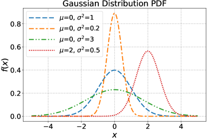
Definition 1.23 (Gaussian or Normal Distribution)
A random variable x is said to follow the Gaussian distribution (a.k.a., a normal distribution) with mean and variance parameters and , denoted by 555Note if two random variables a and b have the same distribution, then we write ., if
The mean and variance of are given by
where is also known as the precision of the Gaussian distribution. Figure 1.1 illustrates the impact of different parameters for the Gaussian distribution.
Suppose are drawn independent, identically distributed (i.i.d.) from a Gaussian distribution of . For analytical simplicity, we may rewrite the Gaussian probability density function as follows:
| (1.4) | ||||
where and .
While the product of two Gaussian variables remains an open problem, the sum of Gaussian variables can be characterized by a new Gaussian distribution. Let x and y be two Gaussian distributed variables with means and variance , respectively. When there is no correlation between the two variables, then it follows that When there exists a correlation of between the two variables, then it follows that
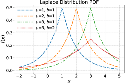
The Laplace distribution, also known as the double exponential distribution, is named after Pierre-Simon Laplace (1749–1827), who obtained the distribution in 1774 (Kotz et al., 2001; Härdle and Simar, 2007). This distribution finds applications in modeling heavy-tailed data due to its tails being heavier than those of the normal distribution, and it is used extensively in sparse-favoring models since it expresses a high peak with heavy tails (same as the regularization term in non-probabilistic or non-Bayesian optimization methods). In Bayesian modeling, when there is a prior belief that the parameter of interest is likely to be close to the mean with the potential for large deviations, the Laplace distribution serves as a suitable prior distribution for such scenarios. {dBox}
Definition 1.24 (Laplace Distribution)
A random variable x is said to follow the Laplace distribution with location and scale parameters and , respectively, denoted by , if
The mean and variance of are given by
Figure 1.2 compares different parameters and for the Laplace distribution.
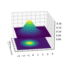
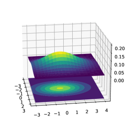
A multivariate Gaussian distribution (also referred to as a multivariate normal distribution) is a continuous probability distribution characterized by a jointly normal distribution across multiple variables. It is fully described by its mean vector (of size equal to the number of variables) and covariance matrix (a square matrix of size equal to the number of variables). The covariance matrix encodes the pairwise relationships among variables through their covariances. The multivariate Gaussian can be used to model complex data distributions in various fields such as machine learning, statistics, and signal processing. We first present the rigorous definition of the multivariate Gaussian distribution as follows. {dBox}
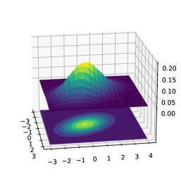
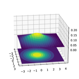
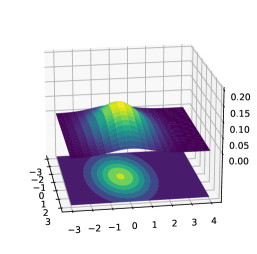
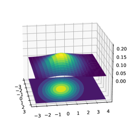
Definition 1.25 (Multivariate Gaussian Distribution)
A random vector is said to follow the multivariate Gaussian distribution with parameters and , denoted by , if
where is called the mean vector, and is positive definite and is called the covariance matrix. The mean, mode, and covariance of the multivariate Gaussian distribution are given by
Figure 1.3 compares Gaussian density plots for different kinds of covariance matrices. The multivariate Gaussian variable can be drawn from a univariate Gaussian density; see Problem 1.0..
The affine transformation and rotation of multivariate Gaussian distribution also follows the multivariate Gaussian distribution. If we assume that , then for non-random matrix and vector .
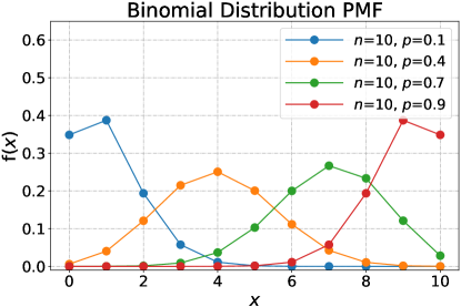
More often than not, we repeat an experiment multiple times independently with two alternative outcomes, say “success” and “failure”, and we want to model the overall number of successes. We are inevitably taken to the binomial distribution if each experiment is modeled as a Bernoulli distribution. This simulates the overall proportion of heads in a run of separate coin flips. {dBox}
Definition 1.26 (Binomial Distribution)
A random variable x is said to follow the binomial distribution with parameter and , denoted by if
The mean and variance of are given by
Figure 1.4 compares different parameters of with for the binomial distribution.
A distribution that is closely related to the Binomial distribution is called the Bernoulli distribution. A random variable is said to follow the Bernoulli distribution with parameter , denoted as , if
with mean and variance , respectively.
Exercise 1.1 (Bernoulli and Binomial)
Show that if with , then we have .
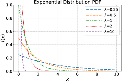
The exponential distribution is a probability distribution commonly used in modeling events occurring randomly over time, such as the time elapsed until the occurrence of a certain event, or the time between two consecutive events. It is a special Gamma distribution (see definition below) with support on nonnegative real values. {dBox}
Definition 1.27 (Exponential Distribution)
A random variable x is said to follow the exponential distribution with rate parameter 666Note the inverse rate parameter is called the scale parameter. In probability theory and statistics, the location parameter shifts the entire distribution left or right, e.g., the mean parameter of a Gaussian distribution; the shape parameter compresses or stretches the entire distribution; the scale parameter changes the shape of the distribution in some manner. , denoted by , if
We will see this is equivalent to , a Gamma distribution. The mean and variance of are given by
The support of an exponential distribution is on . Figure 1.5 compares different parameters for the exponential distribution.
Note that the average is the average time until the occurrence of the event of interest, interpreting as a rate parameter. An important property of the exponential distribution is that it is “memoryless,” meaning that the probability of waiting for an additional amount of time depends only on , not on the past waiting time. Let . Then we have .
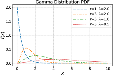
Definition 1.28 (Gamma Distribution)
A random variable x is said to follow the Gamma distribution with shape parameter and rate parameter , denoted by , if
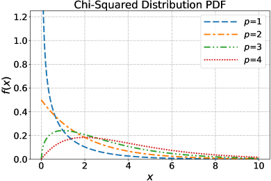
where is the Gamma function, and we can just take it as a function to normalize the distribution into sum to 1. In special cases when is a positive integer, . We will delay the introduction of Chi-squared distribution in Definition 4.1 (p. 4.1) when we discuss the distribution theory. While if , i.e., follows the Chi-squared distribution. Then, , i.e., Chi-square distribution is a special case of the Gamma distribution. The mean and variance of are given by
Figure 1.6 compares different parameters for the Gamma distribution and the Chi-square distribution.
It is important to note that the definition of the Gamma distribution does not constrain to be a natural number; instead, it allows to take any positive value. However, when is a positive integer, the Gamma distribution can be interpreted as a sum of exponentials of rate (see Definition 1.27). The summation property holds true more generally for Gamma variables with the same rate parameter. If and are random variables drawn from and , respectively, then their sum is a Gamma random variable from .
In the Gamma distribution definition, we observe that the Gamma function can be defined as follows:
Utilizing integration by parts , where and , we derive
This demonstrates that when is a positive integer, the relationship holds true.
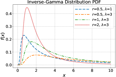
Definition 1.29 (Inverse-Gamma Distribution)
A random variable x is said to follow the inverse-Gamma distribution with shape parameter and scale parameter , denoted by , if
The mean and variance of inverse-Gamma distribution are given by
Figure 1.7(a) illustrates the impact of different parameters and for the inverse-Gamma distribution.
If x is Gamma distributed, then is inverse-Gamma distributed. Note that the inverse-Gamma density is not simply the Gamma density with replaced by . There is an additional factor of . 777Which is from the Jacobian in the change-of-variables formula. A short proof is provided here. Let where and . Then, , which results in for . The inverse-Gamma distribution is useful as a prior for positive parameters. It imparts a quite heavy tail and keeps probability further from zero than the Gamma distribution (see examples in Figure 1.7(a)).
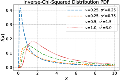
Definition 1.30 (Inverse-Chi-Squared Distribution)
A random variable x is said to follow the inverse-Chi-squared distribution with parameter and , denoted by if
And it is also compactly denoted by . The parameter is called the degrees of freedom, and is the scale parameter. And it is also known as the scaled inverse-Chi-squared distribution. The mean and variance of the inverse-Chi-squared distribution are given by
To establish a connection with the inverse-Gamma distribution, we can set . Then the inverse-Chi-squared distribution can also be denoted by if , the form of which conforms to the univariate case of the inverse-Wishart distribution (see Lu (2023)). And we will observe the similarities in the posterior parameters as well. Figure 1.7(b) illustrates the impact of different parameters and for the inverse-Chi-squared distribution.
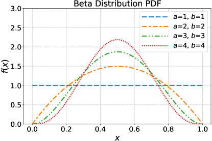
Definition 1.31 (Beta Distribution)
A random variable x is said to follow the Beta distribution with parameter and , denoted by if
where is the Euler’s Beta function and it can be seen as a normalization term. Equivalently, can be obtained by
where is the Gamma function. The mean and variance of are given by
Figure 1.8 compares different parameters of and for Beta the distribution. When , the Beta distribution reduce to a uniform distribution in the range of 0 and 1.
Chapter 1 Problems \adftripleflourishright
-
1.
Eigenvalue Characterization Theorem: Prove that a matrix is positive definite if and only if it possesses exclusively positive eigenvalues. Similarly, a matrix is positive semidefinite if and only if it exhibits solely nonnegative eigenvalues.
- 2.
-
3.
Demonstrate that the vector norm, the matrix Frobenius norm, and the matrix spectral norm satisfy the three criteria outlined in Definition 1.18.
-
4.
Suppose we can generate the univariate Gaussian variable . Show a way to generate the multivariate Gaussian variable , where , , and . Hint: if are i.i.d. from , and let , then it follows that .
- 5.
-
6.
Following the Jacobian in the change-or variables formula for the Gamma distribution and inverse-Gamma distribution, and the definition of the Chi-squared distribution provided in Definition 4.1 (p. 4.1), derive the Jacobian in the change-of-variables formula for the Chi-squared distribution and the inverse-Chi-squared distribution.
Chapter 2 Least Squares Approximations
2.1 Least Squares Approximations
TThe linear model serves as a fundamental technique in regression problems, and its primary tool is the least squares approximation, aiming to minimize the sum of squared errors. This approach is particularly fitting when the goal is to identify the regression function that minimizes the corresponding expected squared error. Over the recent decades, linear models have been used in a wide range of applications, e.g., decision making (Dawes and Corrigan, 1974), time series (Christensen, 1991; Lu, 2017; Lu and Yi, 2022; Lu and Wu, 2022), and in many fields of study such as production science, social science, and soil science (Fox, 1997; Lane, 2002; Schaeffer, 2004; Mrode, 2014).
We consider the overdetermined system , where represents the input data matrix, is the observation vector (targets, responses, outputs), and the sample number is larger than the dimension value . The vector constitutes a vector of weights of the linear model. Normally, will have full column rank since the data from the real world has a large chance to be unrelated or can be made to have full column rank after post-processing (i.e., columns are linearly independent). In practice, a bias term is introduced in the first column of to enable the least squares method to find the solution for:
| (2.1) |
For brevity, we denote and simply by and , respectively, in the following discussions without special mention. In other words, for each data point , we have
It often happens that has no solution. The usual reason is: too many equations, i.e., the matrix has more rows than columns. Define the column space of by and denoted by . Thus, the meaning of has no solution is that is outside the column space of . In other words, the error cannot get down to zero. When the error is as small as possible in the sense of the mean squared error (MSE), is a least squares solution, i.e., is minimized.
In the following sections, we will examine the least squares problem from the perspectives of calculus, linear algebra, and geometry.
2.2 By Calculus
When is differentiable, and the parameter space of is covers the entire space p (the least achievable value is obtained inside the parameter space), the least squares estimate must be the root of . We thus come into the following lemma.
To prove the lemma above, we must show that is invertible. Since we assume has full rank and . is invertible if it has rank , which is the same as the rank of .
Further, let , we have
i.e., . Therefore, . Through the “sandwiching” property, if follows that and . Applying the fundamental theorem of linear algebra in Theorem 2.3.1 (p. 2.3.1), we conclude that and have the same rank.
Applying the observation to , we can also prove that and share the same rank. The ordinary least squares estimate is a result of this conclusion.
Proof [of Lemma 2.2]
Recalling from calculus that a function attains a minimum at a value when the gradient .
The gradient of is . is invertible since we assume is fixed and has full rank. So the OLS solution of is , from which the result follows.
Definition 2.1 (Normal Equation)
We can express the zero gradient of as . The equation is also known as the normal equation. Given the assumption that has full rank with , the invertibility of implies the solution .
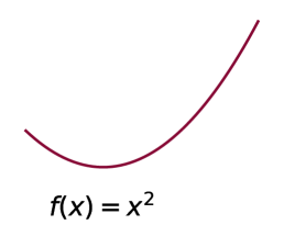
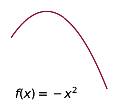
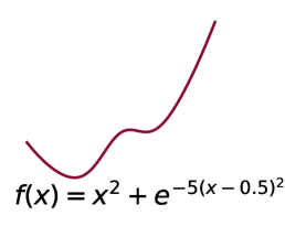
However, we lack certainty about whether the least squares estimate obtained in Lemma 2.2 is the smallest, largest, or neither. A illustrative example is depicted in Figure 2.1. Our understanding is limited to the existence of a single root for the function , which is a necessary condition for the attainment of the minimum value rather a sufficient condition. Further clarification on this issue is provided in the following remark; while an alternative clarification can be established through convex analysis (see Section 2.9). Why does the zero gradient imply the least mean squared error? We refrain from delving into a convex description here, as we will shortly see, to maintain simplicity. However, we directly confirm that the OLS solution indeed minimizes the sum of squared errors. For any , we observe that where the third term is zero from the normal equation, and it also follows that . Therefore, Thus, we show that the OLS estimate indeed corresponds to the minimum, rather than the maximum or a saddle point via calculus approach. In fact, the condition arising from the least squares estimate is also referred to as the sufficiency of stationarity under convexity. When is defined across the entire space p, this condition is alternatively recognized as the necessity and sufficiency of stationarity under convexity.
A further question would be posed: Why does this normal equation magically produce the solution for ? A simple example would give the answer. has no real solution. But has a real solution , in which case makes and as close as possible.
Example 1 (Multiplying From Left Can Change The Solution Set)
Consider the matrix
It can be easily verified that has no solution for . However, if we multiply from left by
Then we have as the solution to . This specific example shows why the normal equation can give rise to the least squares solution. Multiplying from the left of a linear system will change the solution set. The normal equation, especially, results in the least squares solution.
2.3 By Algebra: Least Squares in Fundamental Theorem of Linear Algebra
2.3.1 Fundamental Theorem of Linear Algebra
For any matrix , it can be readily verified that any vector in the row space of is perpendicular to any vector in the null space of . Suppose , then such that is perpendicular to every row of , supporting our claim. This implies the row space of is the orthogonal complement to the null space of .
Similarly, we can also show that any vector in the column space of is perpendicular to any vector in the null space of . Furthermore, the column space of together with the null space of span the entire space of n which is known as the fundamental theorem of linear algebra. Orthogonal Complement and Rank-Nullity Theorem: for any matrix , we have The null space is the orthogonal complement to the row space in p: ; The null space is the orthogonal complement to the column space in n: ; For rank- matrix , , that is, and .
The fundamental theorem contains two parts, the dimension of the subspaces and the orthogonality of the subspaces. The orthogonality can be readily verified as we have shown at the beginning of this section. When the row space has dimension , the null space has dimension . This cannot be easily stated, and we prove it as follows.
Proof [of Theorem 2.3.1] Following the proof of Lemma A (p. A), let be a set of vectors in p that form a basis for the row space. Then, is a basis for the column space of . Let form a basis for the null space of . Following again the proof of Lemma A (p. A), , thus, are perpendicular to . Then, is linearly independent in p.
For any vector , is in the column space of . Thus, it can be expressed as a linear combination of : , which states that , and is thus in . Since is a basis for the null space of , can be expressed by a combination of : , i.e., . That is, any vector can be expressed by and the set forms a basis for p. Thus the dimension sum to : , i.e., . Similarly, we can prove .
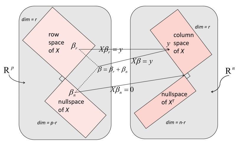
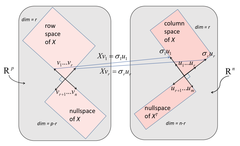
Figure 2.2 demonstrates two pairs of such orthogonal subspaces and shows how takes into the column space. The dimensions of the row space of and the null space of add to . And the dimensions of the column space of and the null space of add to . The null space component goes to zero as , which is the intersection of the column space of and the null space of . The row space component transforms into the column space as .
2.3.2 By Algebra: Least Squares in Fundamental Theorem of Linear Algebra
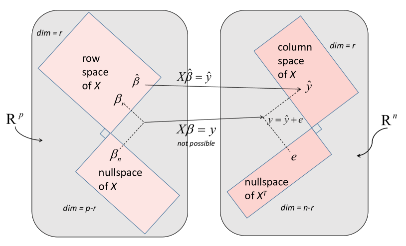
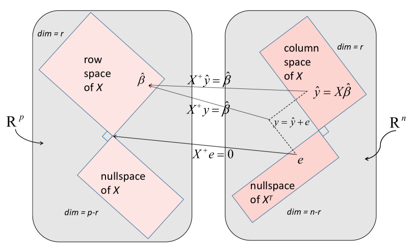
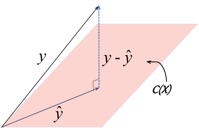
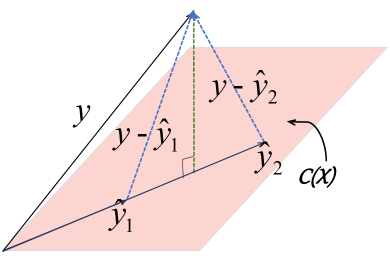
The solution to the least squares problem aims to minimize the error in terms of mean squared error.Since is a combination of the columns of , it remains within the column space of . Therefore, the optimal choice is to select the nearest point to within the column space (Strang, 1993; Lu, 2021b). This point is the projection of onto the column space of . Then the error vector has the minimum length. In other words, the best combination is the projection of onto the column space. The error is perpendicular to the column space. Therefore, is in the null space of (from the fundamental theorem of linear algebra):
which agrees with the normal equation as we have defined in the calculus section. The relationship between and is shown in Figure 2.3, where is decomposed into . We can always find this decomposition since the column space of and the null space of are orthogonal complement to each other, and they collectively span the entire space of n. Moreover, it can be demonstrated that the OLS estimate resides in the row space of , i.e., it cannot be decomposed into a combination of two components—one in the row space of and the other in the null space of (refer to the expression for via the pseudo-inverse of in Section 2.6, where is presented as a linear combination of the orthonormal basis of the row space).
To conclude, we avoid solving the equation by removing from and addressing instead, i.e.,
Prior to delving into the geometric aspects of least squares, we will first elucidate least squares through QR decomposition and singular value decomposition (SVD), as they constitute fundamental components for the subsequent discussions.
2.4 Least Squares via QR Decomposition for Full Column Rank Matrix
In many applications, we are interested in the column space of a matrix . The successive spaces spanned by the columns of are
where is the subspace spanned by the vectors included in the brackets. Moreover, the notion of orthogonal or orthonormal bases within the column space plays a crucial role in various algorithms, allowing for efficient computations and interpretations. The idea of QR decomposition involves the construction of a sequence of orthonormal vectors that span the same successive subspaces. That is,
We illustrate the result of QR decomposition in the following theorem. And in Appendix B (p. B), we provide rigorous proof for its existence.
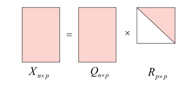
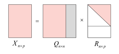
If we obtain the reduced QR decomposition, a full QR decomposition of an matrix with linearly independent columns goes further by appending additional orthonormal columns to , transforming it into an orthogonal matrix. Simultaneously, is augmented with rows of zeros to attain an upper triangular matrix. We refer to the additional columns in as silent columns and the additional rows in as silent rows. The difference between the reduced and the full QR decomposition is shown in Figure 2.4, where silent columns in are denoted in gray, blank entries indicate zero elements, and red entries are elements that are not necessarily zero.
In the least squares solution (Lemma 2.2), the inverse of is not easy to compute, we can then use QR decomposition to find the least squares solution as illustrated in the following theorem.
Proof [of Theorem 2.4] Since is the full QR decomposition of and , the last rows of are zero as shown in Figure 2.4. Then, is the square upper triangular in and Write out the loss function,
where is the first components of , and is the last components of .
Then the OLS solution can be calculated by performing back substitution on the upper triangular system , i.e., .
The inverse of an upper triangular matrix requires floating-point operations (flops). However, the inverse of a basic nonsingular matrix (in our case, the inverse of ) requires flops (Lu, 2021a, 2022c). Consequently, we can mitigate the computational complexity by employing QR decomposition for OLS instead of directly computing the matrix inverse.
To verify Theorem 2.4, given the full QR decomposition of , where and . Together with the OLS solution from calculus, we obtain
| (2.2) | ||||
where and is an upper triangular matrix, and contains the first columns of (i.e., is the reduced QR decomposition of ). Then the result of Equation (2.2) agrees with Theorem 2.4.
In conclusion, through QR decomposition, we directly obtain the least squares result, establishing the content of Theorem 2.4. Additionally, we indirectly validate the OLS result from calculus using QR decomposition. The consistency between these two approaches is evident.
Complexity.
In the least squares solution using QR decomposition, it is unnecessary to compute the orthogonal matrix entirely. This can be observed by performing the Householder algorithm 222which contains two parts: the first one requires flops to obtain the upper triangular matrix , and the second one requires flops to get the orthogonal matrix in the full QR decomposition; see Lu (2021a). on the augmented matrix :
| (2.3) |
where with and . Applying the Householder algorithm allows us to directly compute and . Hence, the complexity of the least squares method using QR decomposition corresponds to the first part of the Householder algorithm, which is approximately flops. The computation cost of obtaining is not included in the final flops count, as it requires flops (not included in the leading term).
Update of least squares problem.
In the context of least squares, each row of and is referred to as an observation. In real-world application, new observation may be received. When performing the optimization process from scratch, obtaining the solution of the least squares problem would require approximately flops. Building upon Equation (2.3), let’s consider a new observation , leading to the following reduction:
Therefore, the updated least squares solution is obtained by transforming into an upper triangular matrix (actually, we transform the left columns of into an upper triangular matrix). This can be done by a set of rotations in the plane, plane, , plane that introduce zero to -th entry of , respectively. The computational cost for this operation is flops Lu (2021a).
LQ Decomposition
We show the existence of the QR decomposition via the Gram-Schmidt process (Appendix B, p. B), in which case we are interested in the column space of a matrix . The successive spaces spanned by the columns of are
The concept behind QR decomposition involves generating a sequence of orthonormal vectors , spanning the same successive subspaces:
However, in many applications (see Schilders (2009)), interest extends to the row space of a matrix , where, abusing the notation, denotes the -th row of . The successive spaces spanned by the rows of are
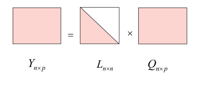
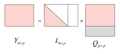
The QR decomposition thus has a counterpart that identifies the orthogonal row space. By applying QR decomposition on , we recover the LQ decomposition of the matrix , where and . The LQ decomposition is helpful in demonstrating the existence of the UTV decomposition in the following section.
Similarly, a comparison between the reduced and full LQ decomposition is shown in Figure 2.5.
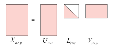
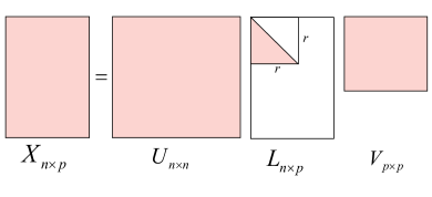
2.5 Least Squares via UTV Decomposition for Rank-Deficient Matrix
The UTV decomposition goes further from QR and LQ decomposition by factoring the matrix into two orthogonal matrices , where and are orthogonal, whilst is (upper/lower) triangular. 333These decompositions fall into a category known as the two-sided orthogonal decomposition. We will see, the UTV decomposition and and singular value decomposition are all in this notion. The resulting supports rank estimation. The matrix can be lower triangular which results in the ULV decomposition, or it can be upper triangular which results in the URV decomposition. The UTV framework shares a similar form as the singular value decomposition (SVD, see Theorem 2.6) and can be regarded as inexpensive alternative to the SVD.
The existence of the ULV decomposition is the consequence of the QR and LQ decomposition.
Proof [of Theorem 2.5] For any rank- matrix , we can use a column permutation matrix (Definition 1.15, p. 1.15) such that the linearly independent columns of appear in the first columns of . Without loss of generality, we assume are the linearly independent columns of and
Let . Since any () is in the column space of , we can find a transformation matrix such that
That is,
where is an identity matrix. Moreover, has full column rank such that its full QR decomposition is given by , where is an upper triangular matrix with full rank, and is an orthogonal matrix. This implies
| (2.4) |
Since has full rank, this means also has full rank such that its full LQ decomposition is given by , where is a lower triangular matrix, and is an orthogonal matrix. Substituting this into Equation (2.4), we have
Let , which is a product of two orthogonal matrices and is also an orthogonal matrix. This completes the proof.
A second way to see the proof of the ULV decomposition is discussed in Lu (2021a) via the rank-revealing QR (RRQR) decomposition and trivial QR decomposition. And we shall not go into the details.
Reduced ULV decomposition.
Now suppose the ULV decomposition of matrix is
Let and , i.e., contains only the first columns of , and contains only the first rows of . Then, we still have . This is known as the reduced ULV decomposition. The comparison between the reduced and the full ULV decomposition is shown in Figure 2.6, where white entries are zero, and red entries are not necessarily zero.
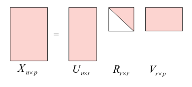
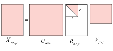
Similarly, we can also claim the URV decomposition as follows.
Again, there is a version of reduced URV decomposition and the difference between the full and reduced URV can be implied from the context, as shown in Figure 2.6. The ULV and URV sometimes are collectively referred to as the UTV decomposition framework (Fierro and Hansen, 1997; Golub and Van Loan, 2013).
The relationship between the QR and ULV/URV is depicted in Figure 2.7. Furthermore, the ULV and URV decomposition can be applied to prove an important property in linear algebra: the row rank and column rank of any matrix are the same (Lu, 2021a). Whereas, an elementary construction to prove this claim is provided in Appendix A (p. A).
We will shortly see that the forms of ULV and URV are very close to the singular value decomposition (SVD). All of the three factor the matrix into two orthogonal matrices. Especially, there exists a set of basis for the four subspaces of in the fundamental theorem of linear algebra via the ULV and the URV. Taking ULV as an example, the first columns of form an orthonormal basis of , and the last columns of form an orthonormal basis of . The first rows of form an orthonormal basis for the row space , and the last rows form an orthonormal basis for :
The SVD goes further that there is a connection between the two pairs of orthonormal basis, i.e., transforming from column basis into row basis, or left null space basis into right null space basis. We will get more details in the SVD section.
Least squares via ULV/URV for rank-deficient matrices.
In Section 2.4, we introduce the LS via the full QR decomposition for full-rank matrices. However, it often happens that the matrix may be rank-deficient. If does not have full column rank, is not invertible. We can then use the ULV/URV decomposition to find the least squares solution, as illustrated in the following theorem.
Proof [of Theorem 2.5] Since is the full UTV decomposition of and . Thus, it follows that
where is the first components of , and is the last components of ; is the first components of , and is the last components of :
And the OLS solution can be calculated by back/forward substitution of the upper/lower triangular system , i.e., . For to have the minimum norm, must be zero. That is,
This completes the proof.
We will shortly find that a similar argument can also be made via the singular value decomposition (SVD) in the following section since SVD shares a similar form as the ULV/URV, both sandwiched by two orthogonal matrices. And SVD goes further by diagonalizing the matrix. Interesting readers can also derive the LS solution via the rank-revealing QR (RRQR) decomposition (Lu, 2021a), and we shall not repeat the details.
A word on the minimum norm LS solution.
For the least squares problem, the set of all minimizers
is convex (Golub and Van Loan, 2013). Given and , then it follows that
Thus, . In the above proof, if we do not set , we will find more least squares solutions. However, the minimum norm least squares solution is unique. For the full-rank case discussed in the previous section, the least squares solution is unique and it must have a minimum norm. See also Foster (2003); Golub and Van Loan (2013) for a more detailed discussion on this topic.
2.6 Least Squares via SVD for Rank-Deficient Matrix
Employing QR decomposition, we factor the matrix into an orthogonal matrix. Unlike the factorization into a single orthogonal matrix, singular value decomposition (SVD) yields two orthogonal matrices, like the UTV decomposition. We illustrate the result of SVD in the following theorem. A rigorous proof for the existence of SVD is presented in Appendix E (p. E).
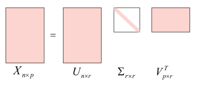
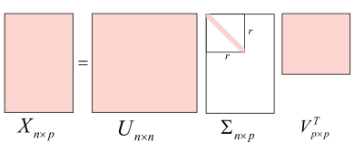
Similar to QR decomposition, a variant of reduced SVD is available (see Theorem E in Appendix E, p. E) achieved by eliminating silent columns in and . The distinctions between reduced and full SVD are highlighted in the blue text of Theorem 2.6. A visual comparison of reduced and full SVD is presented in Figure 2.8, where white entries are zero, and red entries are not necessarily zero.
Eckart-Young-Mirsky Theorem
Suppose we want to approximate matrix with rank by a rank- matrix (). The approximation is measured using the Frobenius norm (Definition 1.20, p. 1.20):
Then we can recover the optimal rank- approximation using the following theorem (Stewart, 1993).
Four Orthonormal Bases in SVD
As previously noted, the construction of SVD yields a set of orthonormal bases for the four subspaces in the fundamental theorem of linear algebra.
Least Squares via SVD for Rank-Deficient Matrices
Returning to the least squares problem, our prior assumption was that has full rank. However, if does not have full column rank, becomes non-invertible. In such cases, we can employ the SVD decomposition of to address the least squares problem with a rank-deficient . The methodology for solving the rank-deficient least squares problem is illustrated in the following theorem.
Proof [of Theorem 2.6] Expressing the loss to be minimized:
Since only appears in , setting for all minimizes the loss above. The result remains the same for any values of . From a regularization point of view, we can set them to be 0 (to get the minimum norm as in the UTV decomposition, Theorem 2.5). This yields the SVD-based OLS solution:
where is known as the pseudo-inverse of . Refer to Appendix 13 (p. 13) for a detailed discussion about the pseudo-inverse, where we also prove that the column space of is equal to the row space of , and the row space of is equal to the column space of .
Proof [of Lemma 2.6] Since is in and it is perpendicular to , and we have shown in Lemma 2.6 that is an orthonormal basis of , then the first components of are all zeros. Therefore, (see also Figure 2.10 where we transfer from into the zero vector by ). Therefore, it follows that .
Furthermore, we have also shown in Lemma 2.6 that is an orthonormal basis of . Thus, is in the row space of .
In the following sections, we will also demonstrate that the vector is the closest point to within the column space of . This point is the (orthogonal) projection of onto the column space of . Then the error vector has the minimum length (norm).
Besides the OLS solution derived from SVD, practical implementations of solutions through normal equations may encounter numerical challenges when is close to singular. In particular, when two or more columns in are nearly co-linear, the resulting parameter values can become excessively large. Such near degeneracies will not be uncommon when dealing with real-world data sets. Addressing these numerical challenges can be effectively achieved through the application of SVD as well (Bishop, 2006).
Least Squares with Norm Ratio Method
Continuing from the previous section’s setup, let be the rank- approximation to the original matrix . Define the Frobenius norm ratio (Zhang, 2017) as
where is the truncated SVD of with the largest terms, i.e., from the SVD of . And is the matrix Frobenius norm (Definition 1.20, p. 1.20). We determine the minimum integer satisfying
as the effective rank estimate , where is the threshold capped at a maximum value of 1, and it is usually set to . Once we have determined the effective rank , we substitute it into Equation (2.5), yielding:
which can be regarded as an approximation to the OLS solution . And this solution corresponds to the OLS solution of the linear equation , where
The introduced filtering method is particularly valuable when dealing with a noisy matrix .
2.7 By Geometry and Orthogonal Projection
As discussed above, the OLS estimate involves minimizing , which searches for an estimate such that is in so as to minimize the distance between and . The nearest point is the projection . The predicted value is the projection of onto the column space by a projection matrix when has full column rank with :
where the matrix is also called the hat matrix as it puts a hat on the outputs.
But what is a projection matrix? Merely stating that is a projection requires elucidation. Before the discussion on the projection matrix, we first provide some basic properties about symmetric and idempotent matrices, which will find extensive application in subsequent sections.
2.7.1 Properties of Symmetric and Idempotent Matrices
Symmetric idempotent matrices exhibit specific eigenvalues, a crucial aspect for the subsequent sections on the distribution theory of least squares.
In Lemma 2.7.1, we will show that the eigenvalues of idempotent matrices (not necessarily symmetric) are 1 and 0 as well, which relaxes the conditions required here (both idempotent and symmetric). However, the method used in the proof is quite useful so we keep both of the claims. To prove the lemma above, we need to use the result of the spectral theorem as follows:
The proof of spectral decomposition, also known as the spectral theorem, is provided in Appendix D (p. D). And now we are ready to prove Lemma 2.7.1.
Proof [of Lemma 2.7.1] Suppose matrix is symmetric idempotent. By spectral theorem (Theorem 2.7.1), we can decompose , where is an orthogonal matrix, and is a diagonal matrix. Therefore, it follows that
Thus, the eigenvalues of satisfy that . We complete the proof.
In the lemma above, we utilize the spectral theorem to prove that the only eigenvalues of any symmetric idempotent matrices are 1 and 0. This trick from spectral theorem is commonly employed in mathematical proofs (see the distribution theory sections in the sequel). Through a straightforward extension, we can relax the condition from symmetric idempotent to idempotent. The only possible eigenvalues of any idempotent matrix are 0 and 1.
Proof [of Lemma 2.7.1] Let denote an eigenvector of the idempotent matrix corresponding to the eigenvalue . That is,
Also, we have
which implies , and is either 0 or 1.
We also demonstrate that the rank of a symmetric idempotent matrix is equal to its trace, a result that will be highly beneficial in the subsequent sections. For any symmetric idempotent matrix , the rank of equals to the trace of .
Proof [of Lemma 2.7.1] From Spectral Theorem 2.7.1, matrix admits the spectral decomposition . Since and are similar matrices, their rank and trace are the same (see Lemma C, p. C). That is,
By Lemma 2.7.1, the only eigenvalues of are 0 and 1. Then, it follows that
.
In the lemma above, we prove the rank and trace of any symmetric idempotent matrix are the same. However, it is rather a loose condition. We here also prove that the only condition on idempotency has the same result. Again, although this lemma is a more general version, we provide both of them since the method used in the proof is quite useful in the sequel. For any idempotent matrix , the rank of equals its trace.
Proof [of Lemma 2.7.1] Any rank- matrix admits CR decomposition , where and with and having full rank (see Appendix A, p. A). 444CR decomposition: Any rank- matrix can be factored as , where contains some independent columns of , and is an matrix used to reconstruct the columns of from the columns of . In particular, is the reduced row echelon form of without the zero rows, and both and have full rank . See Appendix A (p. A) for more details. Then, it follows that
where is an identity matrix. Thus, the trace is
which equals the rank of . The second equality above follows from the fact that the trace is invariant under cyclic permutations.
2.7.2 By Geometry and Orthogonal Projection
Formally, we define the projection matrix as follows:
Definition 2.2 (Projection Matrix)
A matrix is called a projection matrix onto subspace if and only if satisfies the following properties:
(P1). for all : any vector can be projected onto subspace ;
(P2). for all : projecting a vector already in that subspace has no further effect;
(P3). , i.e., projecting twice is equal to projecting once because we are already in that subspace, i.e., is idempotent.
Since we project a vector in n onto the subspace of n, so any projection matrix is a square matrix. Otherwise, we will project onto the subspace of m rather than n. We realize that is always in the column space of , and we would wonder about the relationship between and . And actually, the column space of is equal to the subspace we want to project onto. Suppose , and suppose further that is already in the subspace , i.e., there is a vector such that . Given the only condition above, we have,
That is, condition implies conditions and . Thus, the definition of the projection matrix can be relaxed to only the criterion on .
Intuitively, we also want the projection of any vector to be perpendicular to such that the distance between and is minimal and agrees with our least squares error requirement. This is referred to as the orthogonal projection.
Definition 2.3 (Orthogonal Projection Matrix)
A matrix is called an orthogonal projection matrix onto subspace if and only if is a projection matrix, and the projection of any vector is perpendicular to , i.e., projects onto and along . Otherwise, when is not perpendicular to , the projection matrix is called an oblique projection matrix. See the comparison between the orthogonal projection and oblique projection matrix in Figure 2.11.
Note that in the context of orthogonal projection, it does not imply that the projection matrix itself is orthogonal, but rather that the projection is perpendicular to . This specialized orthogonal projection matrix will be implicitly assumed as such in the subsequent discussion unless explicitly clarified.
Proof [of Lemma 2.7.2] We prove by forward implication and reverse implication separately as follows:
Forward implication.
Suppose is an orthogonal projection matrix, which projects vectors onto subspace . Then any vectors and can be decomposed into a vector lies in ( and ) and a vector lies in ( and ) such that
Since projection matrix will project vectors onto , then and . We then have
where the last equation is from the fact that is perpendicular to , and is perpendicular to . Thus, we have
which implies .
Reverse implication.
For the reverse, if a projection matrix (not necessarily an orthogonal projection) is symmetric, then any vector can be decomposed into . If we can prove is perpendicular to , then we complete the proof. To see this, we have
which completes the proof.
We claimed that the orthogonal projection has a minimum length, i.e., the distance between and is minimized. We rigorously prove this property. Let be a subspace of n and be an orthogonal projection onto . Then, given any vector , it follows that
Proof [of Lemma 2.7.2] Let be the spectral decomposition of the orthogonal projection , be the column partition of , and . Let . Then, from Lemma 2.7.1, the only possible eigenvalues of the orthogonal projection matrix are 1 and 0. Without loss of generality, let and . Then, it follows that
-
is an orthonormal basis of n;
-
is an orthonormal basis of . So for any vector , we have for .
Then we have,
which completes the proof.
Proof [of Lemma 2.7.2] According to the definition of the orthogonal projection, we have . And we could decompose by
This completes the proof.
In conclusion, for determining the OLS solution, we define the projection matrix as idempotent, with the additional condition of symmetry for an orthogonal projection. We illustrate the minimized distance between the original vector and the projected vector through this orthogonal projection.
We proceed further by establishing more connections between the OLS solution and the orthogonal projection.
Proof [of Proposition 2.7.2]
It can be easily verified that is symmetric and idempotent. By SVD of , we have . Let be the column partition of . From Lemma 2.6, is an orthonormal basis of . And in is an matrix with the upper-left part being a identity matrix and the other parts being zero. Apply this observation of into spectral theorem, is also an orthonormal basis of .
Thus, it follows that , and the orthogonal projection is projecting onto , from which the result follows.
The proposition above brings us back to the result we have shown at the beginning of this section. For the OLS estimate to minimize , which searches for an estimate so that is in to minimize the distance between and . An orthogonal projection matrix can project onto the column space of , and the projected vector is with the squared distance between and being minimal (by Lemma 2.7.2).
To repeat, the hat matrix has a geometric interpretation. drops a perpendicular to the hyperplane. Here, drops onto the column space of : . Idempotency also has a geometric interpretation. Additional ’s also drop a perpendicular to the hyperplane. But it has no additional effect because we are already on that hyperplane. Therefore, . This scenario is shown in Figure 2.11(a). The sum of squared error is then equal to the squared Euclidean distance between and . Thus, the least squares solution for corresponds to the orthogonal projection of onto the column space of .
2.7.3 Properties of Orthogonal Projection Matrices
In fact, is also symmetric idempotent. And actually, when projects onto a subspace , projects onto the perpendicular subspace .
Proof [of Proposition 2.7.3] First, is symmetric, since is symmetric. And
Thus, is an orthogonal projection matrix. By spectral theorem again, let . Then, . Hence the column space of is spanned by the eigenvectors of corresponding to the zero eigenvalues of (by Proposition 2.7.1), which coincides with .
For the second part, since and , every column of is perpendicular to columns of . Thus, . For the reverse implication, suppose , then for all . Thus .
Moreover, it can be easily verified when and , then .
A projection matrix with the capability to project any vector onto a subspace is not unique. However, when constrained to orthogonal projection, the projection becomes unique.
Proof [of Proposition 2.7.3] For any vector in n, it can be factored into a vector in and a vector in such that and . Then, we have
such that . Since any vector is in the null space of , then the matrix is of rank 0, and .
Proof [of Proposition 2.7.3] For all , we have . This implies . Thus,
Then for all . That is, the dimension of the null space and the rank of is 0, which results in .
For , both and are symmetric such that , which completes the proof of part 1.
To see the second part, we notice that and
which states that is both symmetric and idempotent. This completes the proof.
From the lemma above, we can also claim that orthogonal projection matrices are positive semidefinite (PSD). Any orthogonal projection matrix is positive semidefinite.
Proof [of Proposition 2.7.3] Since is symmetric and idempotent. For any vector , we have
Thus, is PSD.
As a recap, we summarize important facts about the orthogonal projection matrix that will be extensively used in the next chapters in the following remark. 1. As we assume is fixed and has full rank with . It is known that the rank of is equal to the rank of its Gram matrix, defined as , such that 2. The rank of an orthogonal projection matrix is the dimension of the subspace onto which it projects. Hence, the rank of is when has full rank and : 3. The column space of is identical to the column space of .
2.8 By Geometry with Noise Disturbance
Assume further that the ideal output comes from some ideal function and , where is the noise variable and becomes a random variable. That is, the real observation is disturbed by some noise. In this case, we assume that the observed values differ from the true function by additive noise. This scenario is shown in Figure 2.12. This visual representation provides a comprehensive overview of the problem, setting the foundation for all subsequent developments in this book.
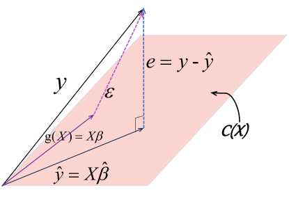
By introducing the noise vector, we provide more facts about the hat matrix: 4. Error vector : projecting onto the perpendicular space is equivalent to projecting onto the perpendicular space. This property can be easily checked from the geometric meaning of and , as shown in Figure 2.12; 5. and are orthogonal, and are orthogonal; 6. Pythagoras: and ; 7. Pythagoras in general: for any orthogonal projection matrix , we have .
The Pythagoras in general can be easily verified that
2.9 Alternating Least Squares*
The explosion of data from advancements in sensor technology and computer hardware poses new challenges for data analysis. The substantial volume of data often contains noise and other distortions, requiring pre-processing for the application of deductive science. For instance, signals received by antenna arrays often are contaminated by noise and other degradations. Effectively analyzing such data requires reconstruction or representation in a manner that minimizes inaccuracies while maintaining certain feasibility conditions.
Moreover, data collected from complex systems often arises from multiple interrelated variables acting together. When these variables lack clear definitions, the information contained in the original data may be overlapping and unclear. By creating a reduced system model, we can achieve a level of accuracy that is close to the original system. The standard approach involves removing noise, reducing the model, and reconstructing feasibility by replacing the original data with a lower-dimensional representation obtained through subspace approximation. Consequently, low-rank approximations or low-rank matrix decompositions play a important role in a wide range of applications.
Low-rank matrix decomposition stands out as a potent technique in machine learning and data mining for representing a given matrix as the product of two or more matrices with lower dimensions. This method captures the essential structure of a matrix while disregarding noise and redundancies. Common techniques for low-rank matrix decomposition include singular value decomposition (SVD), principal component analysis (PCA), multiplicative update nonnegative matrix factorization (NMF), and the alternating least squares (ALS) approach introduced in this section.
For example, in the Netflix Prize competition (Bennett et al., 2007), the objective is to predict the users’ ratings for different movies based on their existing ratings for other movies. We use indices for movies and for users. The rating of the -th user for the -th movie is denoted by . Let be an 555For the purpose of this section, we temporarily assume that the matrix has dimensions ; otherwise, it will be treated as . rating matrix with columns containing ratings provided by the -th user. Note that numerous ratings are missing, and our objective is to accurately predict these absent ratings.
We formally consider algorithms for solving the following problem: Approximating the matrix through factorization into an matrix and a matrix . Typically, is chosen to be smaller than both and , ensuring reduced dimensions for and compared to the original matrix . This dimensional reduction yields a compressed version of the original data matrix. Deciding the appropriate value for is crucial in practice, and its selection is often problem-dependent.
The factorization holds significance; let and be the column partitions of and , respectively. Then, , implying that each column is approximated by a linear combination of the columns of , weighted by the components in . Thus, the columns of can be viewed as containing the column basis of .
To achieve the approximation , a suitable loss function must be established for measuring the distance between and . In this context, we opt for the Frobenius norm (Definition 1.20, p. 1.20) between two matrices, which vanishes to zero if , and the advantage will be evident shortly.
To simplify the problem, let’s first assume the absence of missing ratings. We project data vectors into a lower dimension with in a manner that minimizes the reconstruction error, as measured by the Frobenius norm (assuming is known):
| (2.6) |
where and containing ’s and ’s as rows and columns, respectively. The loss formulation in Equation (2.6) is referred to as the per-example loss. It can be equivalently expressed as
Furthermore, the loss function is convex concerning given , and vice versa. Therefore, we can first minimize it with respect to while keeping fixed, and subsequently minimize it with respect to with fixed. This results in two optimization problems, denoted by ALS1 and ALS2:
This is referred to as the coordinate descent algorithm, wherein we alternate between optimizing the least squares concerning and . Therefore, it is also called the alternating least squares (ALS) algorithm (Comon et al., 2009; Takács and Tikk, 2012; Giampouras et al., 2018). The convergence is guaranteed if the loss function decreases at each iteration, a topic we will delve into further in the following discussions.
Given , Optimizing
Let’s now explore the problem of . When a unique minimum of the loss function exists concerning , we denote it as the least squares minimizer of . With fixed, we can represent as (or more concisely, as ) to emphasize the variable of :
Now, if we define
then the (ALS1) problem an be equivalently transformed into the ordinary least squares problem, aiming to minimize concerning . The solution is then given by
However, it is not advisable to employ this approach for obtaining the result, as computing the inverse of requires flops (Lu, 2021a). Instead, a more direct method to solve the (ALS1) problem is to determine the gradient of concerning (assuming all the partial derivatives of this function exist):
| (2.7) | ||||
where the first equality arises from the definition of the Frobenius norm (Definition 1.20, p. 1.20) such that , and equality () follows from the fact that . When the loss function is a differentiable function of , we can determine the least squares solution using differential calculus. And a minimum of the function must be a root of the equation:
By solving the equation above, we derive the “candidate” update for , which corresponds to the minimizer of :
| (2.8) |
This requires flops to compute the inverse of , a notable improvement compared to flops to get the inverse of (Lu, 2021a). Before we declare a root of the equation above is actually a minimizer rather than a maximizer (that’s why we call the update a “candidate” update), we need to verify the function is convex. In the case where the function is twice differentiable, this confirmation can be equivalently achieved by verifying (see Problem 2.2.):
That is, the Hessian matrix is positive definite (recall the definition of positive definiteness, Definition 1.16, p. 1.16; see Beck (2014)). To see this, we explicitly express the Hessian matrix as
| (2.9) |
which has full rank if has full rank and (Lemma 2.2).
The challenge now is to confirm whether possesses full rank, ensuring the positive definiteness of the Hessian of ; otherwise, we cannot claim the update of in Equation (2.8) reduces the loss (due to convexity), thereby enhancing the matrix decomposition’s approximation of the original matrix through in each iteration. We will shortly come back to the positive definiteness of the Hessian matrix in the sequel, relying on the following lemma. Suppose has full rank with and has full rank with (i.e., ), then the update of in Equation (2.8) has full rank.
Proof [of Lemma 2.9] Since has full rank if has full rank (Lemma 2.2), it follows that has full rank.
Suppose , it implies that . Thus, the following two null spaces satisfy:
Furthermore, suppose is in the null space of such that . And since is invertible, this implies , and
As a result, by “sandwiching,” it follows that
| (2.10) |
Hence, has full rank . Let , and suppose . This implies , and
Similarly, suppose . Since has full rank with the dimension of the null space being 0: , must be zero. The claim follows since has full rank with the row space of being equal to the column space of , where and the . Therefore, is in the null space of if is in the null space of :
By “sandwiching” again,
| (2.11) |
Since has full rank , it follows that .
Therefore,
has full rank .
We complete the proof.
Given , Optimizing
Given fixed, express as (or more concisely, as ) to emphasize the variable of :
A direct approach to solve the optimization of (ALS2) involves finding the gradient of with respect to :
Similarly, the “candidate” update for can be obtained by locating the root of the gradient :
| (2.12) |
Again, it is important to highlight that the provided update is merely a “candidate” update. Further verification is required to determine whether the Hessian is positive definite or not. The Hessian matrix is expressed as follows:
| (2.13) |
Therefore, by analogous analysis, if has full rank with , the Hessian matrix is positive definite.
The proof of Lemma 2.9 is similar to that of Lemma 2.9, and we shall not repeat the details.
Key observation.
Combining the observations in Lemma 2.9 and Lemma 2.9, as long as we initialize and to have full rank, the updates in Equation (2.8) and Equation (2.12) are reasonable since the Hessians in Equation (2.9) and (2.13) are positive definite. Note that we need an additional condition to satisfy both Lemma 2.9 and Lemma 2.9: , i.e., there must be an equal number of movies and users. We will relax this condition in the next section through regularization. We summarize the process in Algorithm 1.
Regularization: Extension to General Matrices
Regularization is a machine learning technique employed to prevent overfitting and enhance model generalization. Overfitting occurs when a model becomes excessively complex, closely fitting the training data but performing poorly on unseen data. To address this issue, regularization introduces a constraint or penalty term into the loss function used for model optimization. This discourages the development of overly complex models, striking a balance between model simplicity and effective training data fitting. Common types of regularization include regularization, regularization, and elastic net regularization (a combination of and regularization). Regularization finds extensive application in machine learning algorithms such as linear regression, logistic regression, and neural networks.
In the context of the alternating least squares problem, we can introduce a regularization term to minimize the following loss:
| (2.14) |
where the gradient with respect to and are given respectively by
| (2.15) |
The Hessian matrices are given respectively by
which are positive definite due to the perturbation introduced by the regularization. To see this, we have
The regularization ensues that the Hessian matrices become positive definite, even if and are rank-deficient. Consequently, matrix decomposition can be extended to any matrix, irrespective of whether or . In rare cases, can be chosen as to obtain a high-rank approximation of . However, in most scenarios, we want to find the low-rank approximation of with . For instance, ALS can be utilized to find low-rank neural networks, reducing the memory usage of neural networks while enhancing performance (Lu, 2021a). Therefore, the minimizers can be determined by identifying the roots of the gradient:
| (2.16) |
The regularization parameters are used to balance the trade-off between the accuracy of the approximation and the smoothness of the computed solution. The selection of these parameters is typically problem-dependent and can be obtained through cross-validation. Again, we summarize the process in Algorithm 2.
Chapter 2 Problems \adftripleflourishright
-
1.
Constrained (Regularized) least squares (CLS). Given , and , we consider the constrained least squares problem:
Show that the constrained least squares (CLS) problem has a unique solution if and only if .
-
2.
Weighted least squares (WLS). Going further from the assumptions in Lemma 2.2, we consider further that each data point (i.e., each row of ) has a weight . This means some data points may carry greater significance than others and there are ways to produce approximate minimzers that reflect this. Show that the value serves as the weighted least squares (WLS) estimator of , where . Hint: find the normal equation for this problem.
-
3.
Restricted least squares (RLS). Going further from the assumptions in Lemma 2.2, we consider further the restriction , where is a known matrix such that has full rank, is a known vector, and is an unknown vector. Show that the value serves as the restricted least squares (RLS) estimator of .
-
4.
Find the restricted weighted least squares estimator.
-
5.
First-order optimality condition for local optima points. Consider the Fermat’s theorem: for a one-dimensional function defined and differentiable over an interval (), if a point is a local maximum or minimum, then . Prove the first-order optimality conditions for multivariate functions based on this Fermat’s theorem for one-dimensional functions. That is, consider function as a function defined on a set . Suppose that , i.e., in the interior point of the set, is a local optimum point and that all the partial derivatives (Definition 1.22, p. 1.22) of exist at . Then , i.e., the gradient vanishes at all local optimum points. (Note that, this optimality condition is a necessary condition; however, there could be vanished points which are not local maximum or minimum point.)
- 6.
-
7.
Two-sided matrix least squares. Let be an matrix and be an matrix. Find the matrix such that is minimized, where is known.
-
Derive the derivative of with respect to and the optimality conditions.
-
Show that one possible solution to the optimality conditions is , where and are the pseudo-inverses of and , respectively.
-
- 8.
- 9.
Chapter 3 Linear Model under Gaussian Disturbance
3.1 From Random Noise to Gaussian Noise
IIn Section 2.1 (p. 2.1), we considered the overdetermined system , where represents the input data matrix with full rank, is the response vector, and the sample number is larger than the dimension value such that the columns of are linearly independent. The vector constitutes a vector of weights of the linear model.
In Section 2.8 (p. 2.8), we assume further that the output comes from some ideal function and , where is the noise variable. That is, the real observation is disturbed by some noise, obtaining the random variable . In this case, we assume that the observed values differ from the true function by additive noise. This scenario is shown in Figure 2.12 (p. 2.12). This visual representation provides a comprehensive overview of the problem.
Suppose further that the noise follows an independent, identically distributed (i.i.d.) Gaussian distribution with zero-mean and variance . For each data point , it is a random variable, as follows:
where we add a bias term . The noise assumption together with the mean squared error (MSE) in the model motivate the likelihood, which gives rise to the maximum likelihood estimator (MLE). To be more concrete, in the case of Gaussian noise, the likelihood function is often expressed as the product of normal density functions. The likelihood function of the observed values under this assumption is
| (3.1) | ||||
which follows a multivariate Gaussian distribution (Definition 1.25, p. 1.25), and represents the probability of observing the given data under the assumed model. To simplify calculations, it is common to work with the log-likelihood function:
| (3.2) |
3.2 Maximum Likelihood Estimator
Perhaps the most important method of parameter estimation is the maximum likelihood estimation. We now give the formal definition of the maximum likelihood estimator. {dBox}
Definition 3.1 (Maximum Likelihood Estimator)
Let be a set of i.i.d. random samples from a distribution with density . Then the maximum likelihood estimator (MLE) 111Estimation method vs estimator vs estimate: Estimation method is a general algorithm to produce the estimator. An estimate is the specific value that an estimator takes when observing the specific value, i.e., an estimator is a random variable and the realization of this random variable is called an estimate. of is such that
where is the likelihood function for the i.i.d. collection. That is, the MLE of can be obtained by
Notice that the likelihood function is a random function, since it depends on the random samples . And the meaning of the likelihood function is the probability of these specific observed samples when the parameter is taken to be equal to rather than the probability of the parameter . In other words, it is the joint density of the sample, but viewed as a function of .
When a unique maximum of the likelihood function exists, we refer to it as the maximum likelihood estimator . If the likelihood is a differentiable function of , we can determine the likelihood estimator using differential calculus. A maximum of the function must be a root of the equation
The solution to the equation provides us with a candidate maximum likelihood estimator. Before we declare a root of this equation is actually an MLE, we need to verify that this corresponds to a maximum, not a minimum. If the likelihood function is twice differentiable, this can be done by verifying the (see Problem 2.2. and 2.2., p.2.2.)
From the likelihood arising from Gaussian disturbances, we can obtain the maximum likelihood estimator for the linear model.
Proof [of Lemma 3.2] Following Equation (3.1), the likelihood of this model under the given parameters and is
and the log-likelihood is given by
Finding the maximum likelihood is equivalent to finding the maximum log-likelihood since the log function is monotone. Thus, the MLE of is
where we remove the constant terms. And we obtain the MLE by solving the following optimization:
Therefore, the MLE of is given by for any value of , which is equal to the OLS estimator.
To see the MLE of variance parameter , we have
By differentiating and setting to zero again, we obtain
It can also be shown that the second partial derivative of the log-likelihood functions are negative, which completes the proof.
In the case of Gaussian noise, the MLE of is equivalent to the OLS estimator since it is exactly the same result of minimizing sum of squares due to error . We will not differentiate the MLE of and the OLS estimator of in the following sections but use the terms interchangeably.
In Section 4.4 (p. 4.4), we will show that the maximum likelihood estimator of variance parameter is a biased estimator of . An unbiased estimator is .
Definition 3.2 (Biased and Unbiased Estimators)
Given the estimator of a parameter , the quantity is called the bias of the estimator with respect to the true parameter . When the bias at some coordinate of is positive, we have overestimation; conversely, when it is negative, we have underestimation; when the bias is zero, we refer to it as an unbiased estimator.
3.3 Laplace Noise
The maximum likelihood estimation framework can be applied to various types of noise models in the context of linear regression. While the Gaussian noise model is commonly used due to its mathematical convenience and certain statistical properties, different noise models may be appropriate depending on the characteristics of the data. Laplace noise with zero-mean is also a common choice:
where for all (Definition 1.24, p. 1.24). The Laplace distribution has heavier tails compared to the Gaussian distribution. Again, the likelihood function for the entire data set is the product of the individual probability density functions:
Once more, we work with the log-likelihood function to simplify calculations:
Therefore, the maximum likelihood estimate of can be obtained by
To find the maximum likelihood estimators, we need to maximize the log-likelihood function with respect to the parameters . Since the root cannot be obtained in closed-forms, this is typically done using optimization techniques.
MLE for .
Taking the partial derivative of with respect to , and setting it to zero:
where is the sign function, which takes the value -1 if the argument is negative, 0 if the argument is zero, and 1 if the argument is positive.
MLE for with .
Taking the partial derivative of with respect to for , and setting it to zero:
MLE for .
Taking the partial derivative of with respect to , and setting it to zero:
That is,
Therefore, the maximum likelihood estimator for the scale parameter is the average absolute deviation between the observed responses and the predicted responses.
Finding analytical solutions for the MLEs in the presence of Laplace-distributed noise may be computationally more involved compared to the Gaussian case. Numerical optimization tools or statistical software packages, e.g., Newton-Raphson iteration and gradient descent, are often used for practical implementations. And we will not go into the details in this book.
Chapter 3 Problems \adftripleflourishright
- 1.
- 2.
-
3.
Uniform noise: Suppose noise points i.i.d. for , i.e., uniformly distributed on and the density function is for . Show that a maximum likelihood estimate of the linear model is any satisfying .
-
4.
Complete the proof for Lemma 3.2 by checking the negativity of the second partial derivatives.
Chapter 4 Distribution Theory of Least Squares
4.1 Distribution Theory of Least Squares
WWe introduce distribution theories relevant to least squares approximation under Gaussian disturbance. Questions may arise regarding the bias of this model and, given a bias, whether we can minimize the variance of this estimator. Notably, we can demonstrate that the bias of the least squares estimator is zero, and its variance is upper-bounded.
When applying the maximum likelihood estimator of (Lemma 3.2, p. 3.2), we can directly compute the expectation of the estimator as (details provided below). Under the least squares probability model, assuming, we also assume that , where follows some probability distribution. Substituting into the estimator of , therefore, we have
The distribution theory of least squares then focuses on this observation.
4.2 Unbiasedness under Moment Assumption
An appetizer of the distribution theory could involve making assumptions solely based on the moments of the noise, rather than specifying its distribution, as follows. Let , where is a random vector of noise 111Note that under the assumed model, the output becomes a random variable , denoted by normal fonts, rather than italics letters.. If we only assume and instead of . Suppose further that is fixed and has full rank with (i.e., rank is ). Then, we have the following moment results: 1. The OLS estimator (i.e., MLE) satisfies and ; 2. The predicted output satisfies and , where is the orthogonal projection matrix with ; 3. The error vector satisfies and .
Proof [of Lemma 4.2] Since the estimator is , and we assume that , we have
Thus, we obtain,
And
And since , we obtain and . 222Given non-random matrix and vector , we have and . Furthermore, since , we have and
which completes the proof.
The lemma establishes that the maximum likelihood estimator of is an unbiased estimator, and the expected error vectors tend towards zero. This underscores the significance of the maximum likelihood method in the realm of point estimation.
4.3 Sampling Distribution of Least Squares under Gaussian Disturbance
Besides understanding the moments of , can we gain insights into its distribution? Analogous to the Gaussian disturbance influencing the likelihood, it also dictates the precise distribution of associated random variables.
Proof [of Lemma 4.3] Since and we assume that , we have
As and are both fixed, thus from the affine transformation of multivariate normal distribution (Lemma 1.1, p. 1.1):
Thus, it follows that
Similarly, for , we obtain:
Considering the error variable , we have , then
where the last equality comes from the fact that is an orthogonal projection onto the perpendicular space of , and this completes the proof.
We further show that, under the same condition, the error variable is independent of the predicted output and the OLS estimator. Let , where . Assume is fixed and has full rank with (i.e., rank is ). Then, the random variable is independent of and ;
Proof [of Lemma 4.3] It is straightforward that
where the second equality is from the fact that , given non-random matrix and .
As , and is the observed data matrix and is fixed, is independent of as well.
This completes the proof.
4.4 Sampling Distribution of Sum of Squares due to Error under Gaussian Disturbance
Another crucial result we will prove is the sum of squares due to error , by which we can get an unbiased estimator of . The distribution is the Chi-square distribution with degree of .
4.4.1 -Distribution, -distribution, and -distribution
Chi-square distribution is a specific case of the Gamma distribution (as introduced in Definition 1.28, p. 1.28). In this context, we provide the formal definitions of the Chi-square distribution, the -distribution, and the -distribution, with a particular emphasis on their close relationship to the Chi-square distribution. Further insights into the connection between the Chi-square distribution and the Gamma distribution will be observed in the sequel.
Though the Chi-squared distribution is a special case of the Gamma distribution, it holds particular significance in statistical theory. {dBox}
Definition 4.1 (Chi-Square Distribution, -Distribution)
Let . Then, follows the Chi-square distribution with degrees of freedom, also known as the -distribution. We write , and it is equivalent to in Definition 1.28 (p. 1.28). The probability density function is given by
The mean, variance of are given by
The function is the Gamma function, and we can just take it as a function to normalize the distribution into sum to 1. In special case when is a positive integer, . Figure 4.1 compares different parameters for the Chi-square distribution.
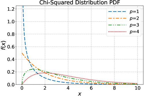
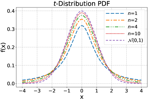
Definition 4.2 (-distribution)
Suppose y and z are independent random variables with and , respectively. Then follows the -distribution with degrees of freedom, denoted by . The probability density function of is given by
And the probability density function of y is given by
Then the probability density function of the -distribution can be obtained by
The probability density function of the -distribution is similar to a normal distribution, both of which are symmetric about 0. And when , -distribution converges to . Figure 4.2 compares different parameters for the -distribution.
Definition 4.3 (-distribution)
The -distribution is the ratio of two Chi-square distributions. Using and to denote numerator and denominator, respectively, we define
And the probability density function is given by
Specifically, if , then . Figure 4.3 compares different parameters for -distribution.
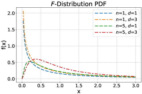
4.4.2 Sampling Distribution
We proceed to demonstrate that certain random variables within the linear model, subject to Gaussian noise, precisely follow a Chi-square distribution. Let , where . Assume is fixed and has full rank with (i.e., rank is ). Then, we have 1. Sum of squares due to error satisfies , where ; 2. An unbiased estimator of is ; 3. The random variables and are independent.
Proof [of Theorem 4.4.2] We realize that . By expressing into :
by which we can rewrite into
By Spectral Theorem 2.7.1 (p. 2.7.1) and Proposition 2.7.1 (p. 2.7.1, the only possible eigenvalues of the hat matrix are 0 and 1), we can express the sum of squares due to error as , where is the spectral decomposition of . Given the fact that rotations on the normal distribution do not affect the distribution (Lemma 1.1, p. 1.1), we can define
Thus, it follows that
where, according to Lemma 2.7.1 (p. 2.7.1),
Therefore, it can be shown that , leading to an unbiased estimator for , denoted by .
As proved in Lemma 4.3, is independent of .
Then, is independent of as well.
This completes the proof.
Degree of Freedom.
To see why (which is the sum of squares due to error divided by ) is an unbiased estimator of , we delve into the concept of degrees of freedom. The unbiased estimator of adjusts the degree of freedom (df) of , while the degree of freedom of is if has full column rank with . It is mysterious why we call as the degree of freedom of . The degree of freedom is the dimension of the space where a vector can stay, i.e., how freely a vector can move. Since is perpendicular to the column space of as shown in Figure 2.12 (p. 2.12). That is, , and is in the null space of which has dimension . So cannot move completely freely in n and loses degree of freedom.
With this unbiased estimator of noise variance , we could answer questions of interest. An example is provided below.
Example 4.4.1
Given any non-random vector , we wish to find the distribution for the following equation:
From , we can find . This makes
And note again . We have
This implies
which is a -distribution 333Suppose and . Then, ., and by which we could answer question of interest.
Moreover, we decompose the noise variance in terms of mean squared error (MSE), from which we could find the minimum MSE estimator of the noise variance.
The above argument shows that will be closer to than when using MSE as a measure. However, is biased and will underestimate on average 444When the bias at some coordinate of is positive, we call it overestimation; when it is negative, we call it underestimation.. This bias raises concerns about the reliability of as an estimator for .
In general, since MSE is a function of the parameter, there will not be just one “best” estimator in terms of MSE. Thus, we should restrict ourselves to finding the “best” estimator in a limited class of estimators. A popular way involves considering only unbiased estimators and selecting the one with the lowest variance. That is, the best unbiased estimator (BUE). Further restrictions to linear estimators lead to the best linear unbiased estimator (BLUE). See Section 6.1 (p. 6.1) for a discussion about the BLUE of .
We should also notice that for any unbiased estimator and of , the linear combination also qualifies as an unbiased estimator for .
In summary, we present various estimators for and in Table 4.1.
| OLS Estimator | MLE | Unbiased Estimator | Minimum MSE Estimator | |
|---|---|---|---|---|
4.5 Learning Curve of Least Squares under Gaussian Disturbance
To differentiate the test data error (the data we do not see), we introduce the concept of in-sample error (also known as the in-sample sum of squares due to error) by for available data samples. Additionally, we define the out-of-sample error (also known as the out-of-sample sum of squares due to error) as the expected squared error of test data, given by . We then derive the expressions for the expected in-sample error and out-of-sample error under the assumption of Gaussian noise disturbance. Let , where . Assume is fixed and has full rank with (i.e., rank is ). Then, we have 1. Expectation of in-sample error: ; 2. Expectation of out-of-sample error: converges to .
Proof [of Lemma 4.5] As a recap, the sum of squares due to error is defined as
where the last two equalities arise from the fact that is symmetric and idempotent. Next, by taking the expectation of the sum of squares due to error with respect to , we obtain:
where the second equality is from the fact that: for random variable and non-random matrix , we have
| (4.1) |
The proof of the equation above is presented in Appendix C (p. C). This expectation aligns with the outcome derived in Theorem 4.4.2, where we establish that with a expectation of . Consequently, we have
Note here, we can directly obtain the expectation of from Theorem 4.4.2. The presented proof offers an alternative approach to determine the expectation of .
For the second part of the claim, given the test input , test output , and test noise , the test error is
Then, the squared test error can be obtained by
1. Taking the expectation of the squared test error with respect to the test input ,
where , and the last two components are again from Equation (4.1).
2. Taking the expectation of the squared test error with respect to the test noise ,
3. Taking the expectation of the squared test error with respect to the input noise ,
| (4.2) | ||||
3.1. For the second part of the above equation, since the trace of a product is invariant under cyclical permutations of the factors, we have:
Let and , then the second part of Equation (4.2) is
where the third equation is from the assumption that , we have 555By the fact that when for non-random variables and . and . And the last equation is from the fact that converges to as , and the trace of a identity matrix is .
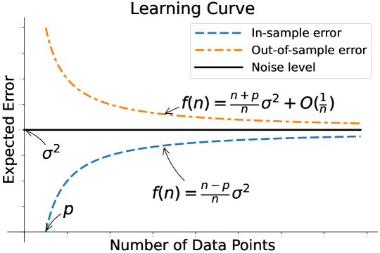
Thus, we obtain the learning curve of least squares under Gaussian noise, as shown in Figure 4.4. When the sample number significantly exceeds the dimension , the expectations of both the in-sample error and the out-of-sample error converge to the noise level.
Chapter 4 Problems \adftripleflourishright
- 1.
-
2.
Prove that if , then .
-
3.
In Lemma 3.2 (p. 3.2), we prove the maximum likelihood estimator of is . By Theorem 4.4.2, we show that the maximum likelihood estimator of is a biased estimator. The unbiased estimator of should be . Given the definitions of overestimation and underestimation in Definition 3.2 (p. 3.2), demonstrate whether the maximum likelihood estimator of in Lemma 3.2 (p. 3.2) is overestimated or underestimated.
Chapter 5 Model Selection and Analysis of Variance
5.1 Model Selection and Analysis of Variance (ANOVA)
QQuadratic forms of normal random vectors are of great importance in many branches of statistics, such as the analysis of variance (ANOVA) in the least squares context. The general idea involves decomposing the sum of squares of the observations into a number of quadratic forms, each corresponding to a specific cause of variation. We will shortly discuss the model selection and the analysis of variance in this chapter; further discussions can be found in Gut (2009b).
5.2 test and ANOVA Decomposition
Consider the observed data matrix with a first column of all 1’s, i.e., the bias term. Then, the column space of correspond to a “line” in the original space (when the first column is not fixed to 1’s). When the input matrix is restricted to a column 111 is an vector with all 1’s., representing the first column of consisting of all 1’s, then is the least squares solution, where and (the observed responses). To see this, if we only select the first column, we should project onto the column space of , and the hat matrix becomes . Then, the projection of is . By Pythagoras’ theorem (Remark 2.8, p. 2.8), we have the following property and definition:
| (5.1) | ||||
| Total sum of squares | ||||
where is the projection of onto the column space of . To see why we have this equality, let be the hat matrix of the whole . We notice that , , and . It can be easily verified that , , and are symmetric and idempotent. Then, it follows that
| (5.2) | ||||
Equation (5.1) is an example of an ANOVA (short for analysis of variance) decomposition. ANOVA decompositions split a variance (or a sum of squares) into two or more components. Typically, these components exhibit orthogonality or adhere to the Pythagorean theorem. {dBox}
Definition 5.1 ( Measure)
We further define the measure,
So is a measure of the percentage of the variance explained by the model. For example, an value of 0.75 can be interpreted as the model explaining 75% of the variance in the dependent variable.
To see why we are comparing the difference between using and using in the model. We should notice that when the data can be expressed by the model, there should be a large difference between the model only having the first parameter and the model having all parameters. The value of is in the range between 0 and 1. When is close to 0, this indicates that the model explains none of the variability; when approaches 1, is very close to , indicating that the model explains all the variability and it is reasonable to use linear model to express the data. However, is already the best we could do under this data set for linear models. When is far from , the data cannot be demonstrated by the linear model. In this situation, we will not go into the variable selection procedure any further (we shall introduce it later).
5.2.1 Degree of Freedom
In Remark 4.4.2 (p. 4.4.2), we claim that has a degree of freedom of such that adjusts the degree of freedom by dividing . Let . We notice that the degree of freedom can be explained as such that the first elements can move freely in (n-1), while the last component is a linear combination of the first ones. We have the following claim: adjusts the degree of freedom of , while the degree of freedom of is if has full column rank with .
| Notation | Degree of freedom | |
|---|---|---|
Moreover, we notice that
where , and are all quadratic forms of with different defining matrices—, and , respectively. The following facts about quadratic forms are important (see Rawlings et al. (2001) for more discussions on quadratic forms):
-
1. All sum of squares can be written as a form of , where is a square symmetric positive definite matrix.
-
2. The degree of freedom associated with any quadratic form is equal to the rank of the defining matrix, which equals its trace when the matrix is idempotent. This agrees with our discussion since , , and .
-
3. Two quadratic forms are orthogonal if the product of their defining matrices is the null matrix .
5.2.2 Estimator and Adjusted Estimator
Previously, we define the measure by
such that is a measure of the percentage of the variance explained by the model. This is equivalent to state that
where is the maximum likelihood estimator of the noise variance as shown in Lemma 3.2 (p. 3.2), and is an estimator of with denoting the -th element of . Thus, we can define the variable
where is the noise variance in the linear model with noise disturbance, and is the variance of output variables . From the discussion on the degree of freedom, we realize that both the two estimators are biased estimators. Thus, estimator is a “biased” estimator of .
The unbiased estimators of and are
| (see Lemma 4.4.2, p. 4.4.2) | (5.3) | ||||
| (see discussion below) |
respectively. We can then define the following adjusted measure for :
which is known as the adjusted estimator of (Theil, 1961).
Unbiased Estimator of from Gaussian Sampling.
Suppose and are random variables from Gaussian distribution, i.e., . Suppose
Then, we have the following proposition.
5.2.3 ANOVA Decomposition
We provide distributional results for the ANOVA decomposition.
Proof [of Lemma 5.2.3] Let , then . Recall that , and it can be easily verified that is symmetric and idempotent (i.e., an orthogonal projection). Then, it follows that
The affine transformation of multivariate normal distribution (Lemma 1.1, p. 1.1) implies that and have the same distribution. That is, and have the same distribution:
By Spectral Theorem 2.7.1 (p. 2.7.1) and Lemma 2.7.1 (p. 2.7.1, the only possible eigenvalues of orthogonal projection matrices are 0 and 1), we can rewrite the sum of squared errors by , where is the spectral decomposition of . By the fact that rotations on the normal distribution do not affect the distribution (Lemma 1.1, p. 1.1), we can define
Thus, it follows that
For , let . Similarly, we have and
Again, the affine transformation of multivariate normal distribution implies and have the same distribution. This results in
Thus, for the spectral decomposition of and , we have
where
Finally, we have
where last equality is from Proposition 2.7.3 (p. 2.7.3) that . This implies and are independent, from which the result follows.
Then, combining Lemma 5.2.3, under the hypothesis , we conclude that
which is independent of and is also known as the test statistic for -test.
Suppose we have the data set , and we observe for this specific data set. Then the value
is known as the -value. We reject the hypothesis if , given some small , say .
A moment of reflexion would reveal that the -value is the chance of extreme cases when the hypothesis is true. If the -value is small, then the hypothesis has a low probability of being correct and the observed data is sufficiently unlikely under the hypothesis, we reject. If not, we fail to reject 222Note that not rejecting is not equal to accepting the hypothesis.. We will provide an example of how this -test works in Figure 5.2 later.
5.2.4 Cochran’s Theorem: An Alternative Proof for Lemma 5.2.3
Cochran’s theorem serves as a fundamental result that is the basis of analysis of variance. If follows a Chi-squared distribution with for , then must be a projection matrix. However, this theorem extends beyond this point. If we can express the total sum of squares as a sum of the sum of squares of each component, and if the degrees of freedom add up, then the matrix must be projections. In the meantime, they are orthogonal to each other and jointly span entire space n (Šemrl, 1996; James, 1952; Wong et al., 1991; Gut, 2009b). We illustrate the Cochran’s theorem as follows, and its proof can be found in Appendix B (p. B).
We notice that and under hypothesis . Since the only eigenvalues of , , and are 1 and 0, they are all PSD. From the proof above, we have , , and , which sum to .
We also notice that is perpendicular to , since is the first column of . That is, , which implies is an eigenvector of corresponding to eigenvalue . In the meantime, we realize that is also an eigenvector of corresponding to eigenvalue . Then,we have
It follows that,
which match the condition 2 in Theorem 5.2.4. As and , thus, , , and and are independent.
5.3 Variable Selection
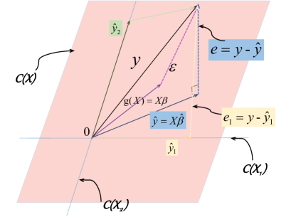
In Section 2.7 (p. 2.7), we show that is the projection of onto the column space of , i.e., . The dimension of has full rank with for . If we decompose into two blocks
where and with . That is, contains the first columns of , and consists of the remaining columns (alternatively, we can choose as random columns from , and as the rest). Then, it follows that
A further question can be posed: Can we set and achieve a comparable reconstructive error to the case when ? Are the last variables redundant for the least squares model? In other words, can the submodel defined by alone perform as effectively as the entire model defined by ?
If we consider only the first variables, the projection of onto the column space of is achieved using the hat matrix . Consequently, the projection of is , and the corresponding error vector is . The situation is shown in Figure 5.1.
For , we define the residual sum of squared error by . Applying Pythagoras’ theorem (Remark 2.8, p. 2.8), we derive the following relationship:
Proof [of Lemma 5.3] For , since and , . And is perpendicular to the column space of . Therefore, .
From Proposition 2.7.3 (p. 2.7.3), we have since . Then . Therefore,
Recall that . Then, the covariance of and is given by
where the second equality is from the fact that for non-random matrices and . Therefore, and are independent.
Furthermore, we realize that
Once again, from Proposition 2.7.3 (p. 2.7.3), we have . Then, we obtain
By Proposition 2.7.3 (p. 2.7.3), we have and . Thus, it follows that
The affine transformation of multivariate normal distribution (Lemma 1.1, p. 1.1) implies that and have the same distribution. That is, and have the same distribution.
By Spectral Theorem 2.7.1 (p. 2.7.1) and Lemma 2.7.1 (p. 2.7.1, the only possible eigenvalues of the hat matrix are 0 and 1), we can rewrite by , where is the spectral decomposition of . From the property that rotations on the normal distribution do not affect the distribution (Lemma 1.1, p. 1.1), we can define
Therefore,
where by Lemma 2.7.1 (p. 2.7.1), we have
This completes the proof.
5.3.1 -test
Then, combining in Theorem 4.4.2 (p. 4.4.2), under the hypothesis , we conclude that
which is the test statistic for -test.
Suppose we have the data set , and we observe for this specific data set. Then we can calculate the -value by
We reject the hypothesis if , for some small , say .
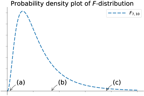
Figure 5.2 illustrates an example of -distribution. At point , the submodel () seems reasonable and the -value is larger than 0.05 such that we cannot reject the hypothesis. At point , the submodel is not reasonable and the -value is smaller than 0.05 such that we reject the hypothesis. At point , things are too good and the data may be preprocessed.
F-test in practice.
In computer programs, we often decompose and by reduced QR decomposition (see Theorem 2.4, p. 2.4). Thus, and , which are the differences of two inner products.
5.3.2 Variable Selection Procedure
In the linear model, we are faced with a large number of possible variables, even though we suspect that a majority of the variables have no relationship to the output . One standard way to assess the confidence involves setting as one column of and as the remaining columns, resulting in a reported -value. And we conduct the variable selection procedure in Algorithm 3. In this procedure, we reduce a potentially large set of variables to a smaller set.
Chapter 5 Problems \adftripleflourishright
-
1.
Under the discussed model, suppose the probability density function for an -test follows , and with a given threshold of , determine the critical value for the test statistic that rejects the hypothesis.
Chapter 6 Best Linear Unbiased Estimator and Minimum Variance Unbiased Estimator
6.1 Best Linear Unbiased Estimator (BLUE)
UUnder the assumption of moment conditions for the noise, as opposed to specifying its distribution, we demonstrate that the ordinary least squares (OLS) estimator exhibits a smaller covariance compared to any other linear unbiased estimator. Through bias-variance decomposition, we establish that the bias terms are universally zero for all unbiased estimators. Consequently, the estimator with the minimal covariance emerges as the optimal choice in terms of mean squared error.
Proof [of Theorem 6.1] Let be any linear estimator, which could be expressed as . Specifically, in the case of OLS, we have . Using the unbiased assumption, we get
which yields . We conclude that the null space of is the entire space p, and thus, . The variance is then
where the first equality is from the fact of covariance under linear transformation by . Then, it follows that
The last equation is from the fact that both and are idempotent. This completes the proof.
The lemma above shows that the OLS estimator achieves the smallest variance compared to other linear estimators. Subsequently, through bias-variance decomposition (as illustrated in the ensuing lemma), we show that the mean squared error between the estimator of and the true parameter is a sum of a bias term and a variance term. Therefore, the OLS estimator achieves the best linear or linear unbiased estimator in the sense of mean squared error to the true parameter .
By combining the Gauss-Markov theorem and the bias-variance decomposition, the theory thus states that if we can find other linear estimators or linear unbiased estimators 111The OLS is unbiased; see Lemma 4.3 (p. 4.3)., their variances must be at least as large as . The OLS estimator is recognized as the best linear estimator (BLE) or the best linear unbiased estimator (BLUE). While we have established that the OLS estimator is the best linear unbiased estimator available “on hand”, one might question whether there exists an imaginary or theoretical estimator with less variance that remains unbiased (not necessarily linear). This will be addressed in the next section.
6.2 Minimum Variance Unbiased (MVU) Estimator
According to the Gauss-Markov theorem, the OLS estimator stands as the best linear unbiased estimator attainable. Yet, the gap between this estimator and the theoretical limit of an unbiased estimator remains unclear. Specifically, we seek insights into the minimum variance achievable for unbiased estimators and the proximity of the OLS variance to this theoretical limit. This question is answered by Cramér-Rao lower bound (CRLB). Note that for this discussion, we assume the additional condition that the noise follows a Gaussian distribution.
The proof of the Cramér-Rao lower bound theorem can be found in Panaretos (2016) and we shall not go into the details.
By repeating the realization of from for times with the same parameters, we find the variance of the OLS estimator attains the bound of CRLB for . We state the conclusion in the following theorem.
Proof [of Theorem 6.2] For simplicity, we only prove the one-dimensional case. Interesting readers can replicate the process to find the proof for the high-dimensional CRLB. Referring again to Equation (3.1) (p. 3.1), the likelihood of this model under and is
For one-dimensional inputs , we have
where the last equation is from the fact that
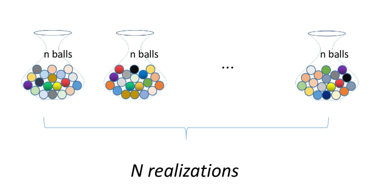
Suppose now we have realizations of from the same and fixed input matrix :
Note the difference between and . For , it means we have fixed samples of on hand (i.e., ). For , we use the same fixed samples to realize different outputs (since we assume Gaussian noise disturbance that gives rises to the likelihood). In other words, for one-dimensional case, we have such ’s, and each , . The situation can be described by coloring balls in a bottle. For each ball, we use different algorithms to decide the color of the ball, e.g., the weight of the ball. Now for the same balls, we repeat the coloring procedure for times, each result will be in a bottle, as shown in Figure 6.1.
So the variance has the relationship , as the bias term for an unbiased estimator.
And since we have proved in Lemma 4.3 (p. 4.3), . Then, repeating times results in . This completes the proof.
It follows that, at least for a large sample size , the OLS estimator of attains a performance, which is equal to theoretical optimal. This explains why the method of OLS is so central to linear model estimation.
Chapter 6 Problems \adftripleflourishright
-
1.
Prove the Cramér-Rao lower bound theorem.
Chapter 7 Generalized Linear Model (GLM)
7.1 Generalized Linear Model (GLM)
WWe will briefly introduce the generalized linear model (GLM) in this section. In Section 9.1 (p. 9.1), the Bayesian approach for linear models will be discussed (Broemeling, 2017). While there exists a Bayesian perspective on the GLM topic (Dey et al., 2000), it will not be addressed here for simplicity.
Previously, we assumed that , where and is fixed and has full rank with , i.e., rank is :
| (7.1) |
Now, let’s consider the case where the covariance matrix of the noise vector is not diagonal:
where is known and positive definite. It can be verified that . And we can decompose into symmetric square roots . Let , we have
In other words,
| (7.2) |
Comparing the forms of Equation (7.1) and Equation (7.2), we can then use the maximum likelihood estimator for the linear model and ordinary least squares on by projecting onto the column space of and get the estimator for . For example, following Lemma 3.2 (p. 3.2), the maximum likelihood estimators of and are
respectively. Similarly, other estimators in Table 4.1 (p. 4.1) can be obtained accordingly.
7.2 Orthogonal Projection in Generalized Linear Model
We previously showed that the orthogonal projection matrix
is an orthogonal projection onto the subspace . Now, we also observe that
is the orthogonal projection onto the subspace . This implies
is also an orthogonal projection onto the subspace .
Before delving into the properties of orthogonal projection in the generalized linear model, it is essential to clarify the term “symmetry.” While a matrix is considered symmetric if , a distinct definition of symmetry is employed concerning inner product considerations.
The definition of a inner product should satisfy three criteria. {dBox}
Definition 7.1 (Inner Product)
In most cases, the norm can be derived from the vector inner product (the inner product of vector is given by ), which satisfies three criteria as follows
-
Commutativity. for any .
-
Linearity. for any and .
-
Positive definiteness. for any , and if and only if .
Then, the notion of symmetry can be defined as follows. {dBox}
Definition 7.2 (Symmetric in terms of Inner Product)
A matrix is called symmetric if for all , such that .
-
1.
Considering the inner product , symmetric means .
-
2.
Given a positive definite matrix , considering the inner product , symmetric means . In this case, we have the generalized norm , also known as the -norm.
Given this definition of symmetry based on the inner product, we can extend the concept of orthogonal projection to be symmetric in terms of inner product, essentially a generalized orthogonal projection. Then, we can check that is symmetric in terms of such that
for all .
Proof [of Lemma 7.2] We prove is an orthogonal projection by showing that it is idempotent and symmetric, and it projects onto the column space of . It can be readily verified that
and
Since , the columns of are combinations of the columns of , thus . By Lemma 2.7.1 (p. 2.7.1), we have
where the third equality is from the fact that the trace of a product is invariant under cyclical permutations of the factors: if all , , and exist.
Thus, the rank of equals the rank of such that .
And the minimum distance in orthogonal projection Lemma 2.7.2 (p. 2.7.2) can be extended to the generalized norm version. Let be a subspace of n and be a generalized orthogonal projection with respect to onto subspace . Then, it follows that
Proof [of Lemma 7.2] We find that , , and are all symmetric (with respect to the first inner product in Definition 7.2, i.e., the traditional symmetry). Therefore, they all admit a spectral decomposition. By trial and error, the right way is to decompose
where is the column partition of , and contains the eigenvalues of . Let . We notice that is symmetric and idempotent such that its only possible eigenvalues are 1 and 0 by Lemma 2.7.1 (p. 2.7.1). Without loss of generality, let and . Then, we have
-
is an orthonormal basis of n;
-
is an orthonormal basis of , which is the subspace rotated by . So for any vector , let , we have for .
Again, let , we have,
which completes the proof.
This orthogonal projection in the context of the generalized linear model is also referred to as generalized least squares (GLS), resembling the projection used in ordinary least squares. In previous discussions, for any orthogonal projection matrix , we established Pythagoras’ theorem and the orthogonal property in ordinary least squares (i.e., with inner product denoted by ):
Analogously, in the generalized orthogonal projection, we have
and
Weighted least squares (WLS).
7.3 Equivalence between OLS and GLS
In Lemma 2.7.2 (p. 2.7.2), we prove that for any orthogonal projection , the inequality holds for all . In the context of generalized least squares, the analogous result holds for any generalized orthogonal projection matrix : with positive definite . Despite the general distinction between the two estimates, we demonstrate that, under specific conditions, they are equivalent.
Proof [of Theorem 7.3] Suppose . Then for all , we must have
which implies
By taking transpose, we have
Since and are nonsingular, only transforming from one basis to another and leading to .
For the reverse, suppose , there must be a nonsingular matrix such that (columns of are combinations of columns of , and the combinations are given by ). That is . Then, we have
which completes the proof.
Chapter 7 Problems \adftripleflourishright
-
1.
Given a positive definite matrix , show that for all is a valid norm that satisfies the three criteria in Definition 7.1.
Chapter 8 Large-Sample Properties in OLS Estimator*
8.1 Convergence Results*
WWe introduce fundamental convergence results and asymptotic theories in this section. Comprehensive discussions and proofs on this topic can be found in Cameron and Trivedi (2005); Panaretos (2016); Shao (2003); Hansen (2007); Yu (2021); Gut (2009a); Wooldridge (2010); Hayashi (2011); Bickel and Doksum (2015).
8.1.1 Convergence*
We first define the convergence in distribution as follows: {dBox}
Definition 8.1 (Convergence in Distribution)
Let be a sequence of distribution functions and be a distribution function on . That is, the distribution function are
and
We say that converges in distribution to , and write (or ) if and only if
for all that are continuity points of .
Definition 8.2 (Convergence in Probability)
A sequence of random variables is said to converge in probability to random variable y as , denoted as , if for any ,
The convergence in probability tells more than the convergence in distribution from the definitions above. There are several other convergence concepts in probability theory, such as convergence in -mean, convergence almost surely. However, these concepts will not be addressed in this context.
Example 8.1.1
Let be a sequence of random variables with
Then , but .
Proof [of Lemma 8.1.1] For (1). let be any continuity point of and . Then, we have
| (8.1) | ||||
where the inequality comes from the fact that contains . Moreover, it follows that
where the inequality comes from the fact that contains . This implies
| (8.2) |
Combining Inequality (8.1) and Inequality (8.2), we have
Since we assume . Then, when , we have
which yields (1).
For (2). we have
Since , we have and as and . Therefore,
which completes the proof.
Definition 8.3 (Joint Convergence)
Let be a sequence of random vectors of p, and be a random vector of p. Define the distribution function
and
for . Then we say converges in distribution to as if for every continuity point of we have
And denoted by .
When an estimator converges in probability to the true value as the sample size diverges, we say that the estimator is consistent. In mathematical language, we have the following definition.
Definition 8.4 (Consistency)
An estimator of constructed on the basis of a sample of size is said to be consistent if as .
Consistency a desirable property for an estimator. When the sample size is large enough, the estimator will be arbitrarily close to the true value with high probability. Moreover, the concentration of an estimator around the true parameter can always be bounded using the mean squared error.
Proof [of Lemma 8.1.1] Let . Since , applying Markov’s inequality (see Appendix D, p. D) yields
This completes the proof.
Both biased and unbiased estimators can be consistent (an example can be found in Theorem 8.3.1). Regarding mean squared error (MSE), both biased and unbiased estimators can achieve an MSE approaching zero as the sample size becomes sufficiently large.
8.1.2 Asymptotic Theory*
Five tools, along with their extensions, play a crucial role in asymptotic theory. These tools include the weak law of large numbers (WLLN), the central limit theorem (CLT), the continuous mapping theorem (CMT), Slutsky’s theorem, and the Delta method.
The key observation in WLLN lies in the scaling by , which renders the variance as such that it converges to zero. Consequently, the mean converges to (or in the multi-dimensional case).
The CLT is stronger than the WLLN2 as implies (since in CLT). However, does not provide any information about .
In addition to the common CLT, the following theorem represents a more general version of the central limit theorem that will be often useful. Let be a sequence of i.i.d. real random variables with and . Let be a sequence of real constants. If then
The CMT was proved by Mann and Wald (1943) and is sometimes referred to as the Mann-Wald Theorem. Note that the CMT allows the function to be discontinuous but the probability of being at a discontinuity point is zero. For example, the function is discontinuous at . But if , then such that .
An important application of Slutsky’s theorem is illustrated below:
Example 8.1.2
Suppose and . Then .
The Delta method is a direct consequence of Slutsky’s theorem and CMP, and it allows us to transform CLT. Let , where for all and . Let be differentiable at . Then, , provided that . Then in the theorem above is usually constructed to be such that as . The Delta method implies that, asymptotically, the randomness in a transformation of is completely controlled by that in .
Proof [of Theorem 8.1.2] By Taylor’s expansion (Appendix E, p. E) around , we have
where lies between and such that
where the convergence is from the Slutsky’s theorem. Therefore, we have . By applying CMT, we have . Therefore,
where the convergence is from the Slutsky’s theorem.
Example 8.1.3
Suppose are i.i.d. random variables with mean and variance . Let . By CLT, we have
Given a continuously differentiable function , the Delta method implies that
Suppose further that is a sequence of random variables such that . Then, by Slutsky’s theorem, we obtain
Apart from the five basic weapons, the following Cramér-Wold Device is also very useful. Let be a sequence of random vectors in d, and be a random vector in d. Then,
8.2 Assumptions Restated*
For large sample asymptotic results of least squares estimators, we restate the assumptions as follows: OLS.0 (random sampling): (), are i.i.d. OLS.1 (full rank): . OLS. . OLS.2 (first moment): , i.e., and . OLS. with . OLS.3 (second moment): , where is the noise associated with input OLS. (homoskedasticity): . OLS.4 (normality): .
Assumption OLS.2 is equivalent to stating (linear in parameters) and (zero conditional mean). And Assumption OLS.2 is stronger than Assumption OLS2.2. Moreover, Assumption OLS.3.2 is stronger than Assumption OLS.3 since OLS3.2 implies the independence between and . The linear model under Assumption OLS.3.2 is called the homoskedastic linear regression model. In most of our discussions in the previous sections, we assume OLS.0, OLS.1, OLS.2, OLS.3.2, OLS.4. That is
| y | |||
However, if , i.e., the noise variance depends on , we say is heteroskedastic.
8.3 Asymptotics for the OLS Estimator*
8.3.1 Consistency*
The assumptions OLS2.2 and OLS.3 in this context appear less stringent compared to those employed in earlier sections for obtaining the estimator . A stronger assumption by OLS.2 and OLS.3.2 can yield the same result.
Proof [of Theorem 8.3.1] Express the OLS estimator as
Then, it is sufficient to show the consistency by proving .
For , since ’s are i.i.d. (OLS.0), as implied in OLS.1.2 and by applying WLLN1. This implies .
For , similarly, since ’s are i.i.d. (OLS.0), we have by applying WLLN1 if we have . To see why , we have
by Cauchy-Schwarz inequality (see Appendix D, p. D), and which is finite by Assumption OLS1.2 and OLS.3. Then, can be expressed as
by applying Slutsky’s theorem.
Proof [of Theorem 8.3.1] We realize that
Thus, it follows that
by applying the WLLN1, Theorem 8.3.1, and the Slutsky’s theorem.
For , it follows that
by the Slutsky’s theorem.
From the theorem above, we find two different estimators can be both consistent. That is, when sample size is large enough, and will be close.
As mentioned earlier, both biased and unbiased estimators can exhibit consistency.
The theorem underscores that both the biased estimator and the unbiased estimator demonstrate consistency.
8.3.2 Asymptotic Normality under Noise Moment Assumption*
To study the approximate sampling distribution of OLS under the moment assumption, we impose the following additional assumption:
-
Assumption OLS.5: .
Under the moment assumption, we only assume and instead of . We proved that the OLS estimator of is unbiased such that and in Section 4.2 (p. 4.2), and the sampling distribution of is in Lemma 4.3 (p. 4.3) if we assume further that the noise is from a Gaussian distribution: . But what can we say about the sampling distribution of when is not from Gaussian?
We prove that, subject to specific conditions (OLS.5), we can approximate the sampling distribution of the ordinary least squares estimator under the moment assumption. Let be a sequence of design matrices, and be a sequence of vectors. For each element, let . If 1. OLS.0 (random sampling): (), are i.i.d. 2. OLS.1.2: has full rank for all . 3. OLS.2 and OLS.3, the moment assumption: and for all . That is, for each -th element , we have and . 4. OLS.5: . Then the ordinary least squares estimator satisfies where is a identity matrix.
Proof [of Lemma 8.3.2] Recall that . Then, we have . Let be a unit-length vector and such that
where is the -th row of for . Then, we have
That is, is a unit-length random vector. Moreover, according to Schwarz matrix inequality (see Appendix D, p. D), we have
Therefore,
Thus, by weighted sum central limit theorem in Theorem 8.1.2, it follows that
That is,
Since we assume is a unit-length vector, then if , we have . By Cramér-Wold device (see Theorem 8.1.2), this implies that
We complete the proof.
This convergence result can be interpreted as for large enough, by the affine transformation of multivariate normal distribution, we have
and
8.3.3 Asymptotic Normality under Higher Moment Assumption*
To further study the approximate sampling distribution of OLS under the moment assumption, we impose the following additional assumption:
-
Assumption OLS.6 and .
Proof [of Theorem 8.3.3] Following from Theorem 8.3.1, we have
By applying Cauchy-Schwarz inequality, we have
where the second inequality is from the Schwarz matrix inequality (see Appendix D, p. D), and the last inequality is from Assumption OLS.6. Therefore, according to the CLT and OLS.2.2, we have
Again, we have . Thus,
by Slutsky’s theorem and is symmetric.
Compared to Theorem 8.3.2 (which is homoskedastic), we have a similar result in the Theorem 8.3.3 above (which is heteroskedastic). However, in Theorem 8.3.3, we do not assume the moment assumption on the noise: and . This results in the difference between the covariance matrices of in the two theorems.
In the homoskedastic model, reduces to , which is the same as that in Theorem 8.3.2. 111 is known as the homoskedastic covariance matrix. But the result in Theorem 8.3.3 is more general.
Chapter 8 Problems \adftripleflourishright
-
1.
Given the central limit theorem, prove the validity of the weighted sum central limit theorem.
-
2.
Suppose and with , show that .
Chapter 9 The Bayesian Approach
9.1 The Bayesian Approach
IIn modern statistics, Bayesian approaches have become increasingly more important and widely used. Thomas Bayes came up with this idea but died before publishing it. Fortunately, his friend Richard Price carried on his work and published the work in 1764. In this section, we describe the basic ideas of the Bayesian approach, employing the Beta-Bernoulli model as an appetizer to illustrate the advantages of Bayesian models. Moreover, we present powerful Bayesian techniques for linear models and their connection to ordinary least squares.
Let be the observations of data points, and suppose they are independent and identically distributed, with the probability parameterized by . Note that the parameters might contain hidden variables; for example, the latent variables in a mixture model to indicate which cluster a data point belongs to (Lu, 2021c).
The idea of the Bayesian approach involves assuming a prior probability distribution over with hyper-parameters (i.e., )—a distribution representing the plausibility of each possible value of before observing the data. Consequently, to make inferences about , we simply consider the conditional distribution of given the observed data. This is referred to as the posterior distribution, since it represents the plausibility of each possible value of after seeing the data. Mathematically, this is expressed via the Bayes’ theorem,
| (9.1) | ||||
where is the observed data set, and means is proportional to . In other words, we say the posterior is proportional to the product of the likelihood and the prior:
which computes a distribution over the unknown parameters, allowing for the quantification of uncertainties.
Moreover, though we will not use any hierarchical models in this book, Bayesian modeling is often more flexible, allowing for the specification of complex hierarchical models. This flexibility is advantageous in cases where the underlying data-generating process is intricate.
In a nutshell, the Bayesian approach entails assuming a prior distribution for any unknowns ( in our case) and subsequently applying probability rules to address specific questions of interest. For example, when we find the parameter based on the maximum posterior probability of , we turn to the maximum a posteriori (MAP) estimator.
Definition 9.1 (Maximum a Posterior Estimator)
Maximum a posteriori (MAP) estimate is the parameter value that maximizes the posterior distribution. The MAP estimate balances information from the prior distribution with information from the likelihood. The influence of the prior is stronger when the likelihood provides less information, and vice versa.
9.2 An Appetizer: Beta-Bernoulli Model
We formally present a Beta-Bernoulli model to show how the Bayesian approach works. The Bernoulli distribution models binary outcomes, i.e., outputting two possible values (conventionally denoted as 0 and 1). The likelihood under this model is just the probability mass function of the Bernoulli distribution:
That is,
where is the probability of outputting 1 and is the probability of outputting 0. The mean of the Bernoulli distribution is . Suppose are drawn i.i.d. from . Then, the likelihood under the Bernoulli distribution is given by:
which is a distribution on and is called the likelihood function on .
The prior distribution within this model follows the probability density function of the Beta distribution:
where represents the Euler’s beta function, serving as a normalization term. And is a step function that has a value of 1 when and 0 otherwise (when or ). Figure 1.8 (p. 1.8) compares different parameters for the Beta distribution. Specifically, when , the Beta distribution reduces to a uniform distribution in the support of .
We put a Beta prior over the parameter of the Bernoulli distribution. The posterior is obtained by
We find that the posterior distribution shares the same form as the prior distribution. When this happens, we call the prior conjugate prior. The conjugate prior has a nice form such that it is easy to work with for computing the posterior probability density function and its derivatives, and for sampling from the posterior. The use of conjugate priors offers an advantage in maintaining the mathematical form of the prior during the updating process. Consequently, this yields closed-form expressions for the posterior distribution, eliminating the necessity for complex numerical methods.
Example 9.2.1 (Amount of Data Matters)
Bayesian methods can be advantageous in cases of small sample sizes or sparse data, where traditional frequentist methods may encounter difficulties. Suppose we have three observations for the success in Bernoulli distribution:
-
1.
10 out of 10 are observed to be success (1’s);
-
2.
48 out of 50 are observed to be success (1’s);
-
3.
186 out of 200 are observed to be success (1’s).
So, what is the probability of success in the Bernoulli model? Normal answer to case 1, 2, and 3 are 100%, 96%, and 93%, respectively. But an observation of 10 inputs is rather a small amount of data, and noise can make it less convincing.
Suppose we put a (a uniform distribution, see Figure 1.8, p. 1.8) prior over the Bernoulli distribution. The posterior probability of success for each case would be , , and , respectively. Therefore, we find the case 1 has less probability of success compared to case 2.
A Bayesian view of the problem naturally incorporates the amount of data as well as its average. This special case shown here is also called the Laplace’s rate of succession (Ollivier, 2015). Laplace’s “add-one” rule of succession modifies the observed frequencies in a sequence of successes and failures by adding one to the observed counts. This improves prediction by avoiding zero probabilities and corresponds to a uniform Bayesian prior on the parameter.
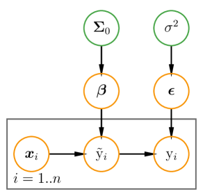
9.3 Bayesian Linear Model: Zero-Mean Prior
We now present the Bayesian methods for linear models. Assume where and is fixed. As discussed in Section 3 (p. 3), this additive Gaussian noise assumption gives rise to the likelihood. Let be the observations of data points, and contains the corresponding outputs, the joint likelihood is given by
Suppose we specify a multivariate Gaussian prior with zero-mean over the weight parameter
The graphical representation of this Bayesian linear model is shown in Figure 9.1. Applying Bayes’ theorem “,” we get the posterior
where and . Therefore, the posterior distribution is also a multivariate Gaussian distribution (same form as the prior distribution, i.e., a conjugate prior):
A word on the notation.
Note that we use to denote the posterior mean and posterior covariance in the zero-mean prior model. Similarly, the posterior mean and posterior covariance in semi-conjugate prior and full conjugate prior models will be denoted by and , respectively (see sections below).
Connection to OLS.
In the Bayesian linear model, there is no general requirement for to have full rank, ensuring that to be nonsingular. Note further that if we assume has full rank, in the limit, when , , in which case, maximum a posteriori (MAP) estimator from the Bayesian linear model aligns with the ordinary least squares estimator. And the posterior is , which shares similar form as the OLS estimator under the Gaussian disturbance (see Lemma 4.3, p. 4.3).
Connection to ridge regression.
We realize that when we set , we obtain and . Since , the MAP estimate of becomes , which shares the same form as ridge regression by letting . Therefore, ridge regression emerges as a special case of the Bayesian linear model with a zero-mean prior. The Bayesian perspective provides a meaningful interpretation for ridge regression—identifying the mode of the posterior distribution.
9.3.1 Zeller’s -Prior and Variable Transformation
As an illustrative example, consider the analysis of an individual’s weight based on human characteristics, where a variable in represents the person’s height in meters. If the variable is now given in centimeters, the model remains unchanged, and we can adjust by dividing the corresponding parameter in by 100 (to convert centimeters back to meters). More generally, suppose the input matrix is transferred by given a matrix , in which case the model parameter is . Then, we have
According to the principle of invariance, the posterior distributions of and should be the same. As shown previously, for , the posterior is
Similarly, for , the posterior distribution of is
Following the principle of invariance, a simple calculation can show that this condition is met if , where is a hyper-parameter. A popular specification of is to relate it to the noise variance by . This is called the Zeller’s -prior (Zellner, 1986). Following the Bayesian linear model with a zero-mean prior, the posterior of is
where and .
9.4 Bayesian Linear Model: Semi-Conjugate Prior Distribution
We will use Gamma distribution as the prior for the inverse variance (precision) parameter of a Gaussian distribution. The rigorous definition of the Gamma distribution can be found in Definition 1.28 (p. 1.28). The choice of the Gamma distribution as the prior for precision is motivated by the rationale provided in Kruschke (2014): Because of its role in conjugate priors for normal likelihood function, the Gamma distribution is routinely used as a prior for precision (i.e., inverse variance). But there is no logical necessity to do so, and modern Markov chain Monte Carlo (MCMC) methods permit more flexible specification of priors. Indeed, because precision is less intuitive than standard deviation, it can be more useful to give standard deviation a uniform prior that spans a wide range.
Same setting as Section 9.3, we now consider as a variable rather than a fixed value. Again, the likelihood function is given by
We specify a non-zero-mean Gaussian prior over the weight parameter and a Gamma prior over the inverse variance parameter :
| (9.2) | ||||
where the changes from the previous descriptions are highlighted in blue text. The graphical representation of this Bayesian linear model is shown in Figure 9.2.
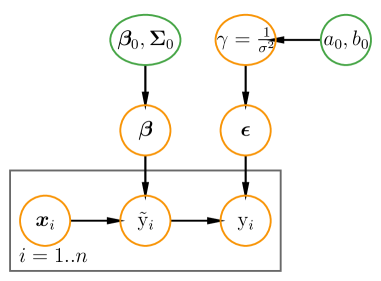
Step 1, conditioned on .
Then, given , by Bayes’ theorem “”, we obtain the conditional posterior density of :
where the parameters are
Therefore, the conditional posterior density is also a Gaussian distribution:
Step 2, conditioned on .
Given , again, by Bayes’ theorem, we obtain the posterior
Therefore, the conditional posterior of follows a Gamma distribution:
| (9.3) |
9.4.1 Gibbs Sampling with Two Variables
Gibbs sampling was introduced by Turchin (Turchin, 1971), and later introduced by brothers Geman in the context of image restoration (Geman and Geman, 1984). The Geman brothers named the algorithm after the physicist J. W. Gibbs, some eight decades after his death, in reference to an analogy between the sampling algorithm and statistical physics.
Gibbs sampling is applicable when the joint distribution is not known explicitly or is difficult to sample from directly, but the conditional distribution of each variable is known and easy to sample from. A Gibbs sampler generates a draw from the distribution of each parameter or variable in turn, conditional on the current values of the other parameters or variables. Therefore, a Gibbs sampler is a componentwise algorithm. In our example from Section 9.1, given some data and a probability distribution parameterized by . We can successively draw samples from the distribution by sampling from
| (9.4) |
where is all current values of in -th iteration except for . If we sample long enough, these values will be random samples from the distribution .
In deriving a Gibbs sampler, it is often helpful to observe that
| (9.5) |
The conditional distribution is proportional to the joint distribution. We will get a lot of benefits from this simple observation by dropping constant terms from the joint distribution (relative to the parameters we are conditioned on).
Shortly, as a simplified example, given a joint probability distribution , a Gibbs sampler would draw , then iteratively. The procedure defines a sequence of realization of random variables and :
which converges to the joint distribution . More details about Gibbs sampling can be found in Turchin (1971); Geman and Geman (1984); Müller and Quintana (2004); Rencher and Schaalje (2008); Hoff (2009); Gelman et al. (2013); Kruschke and Liddell (2018).
By this Gibbs sampling method, we can construct a Gibbs sampler for the Bayesian linear model with semi-conjugate prior in Section 9.4:
-
1.
Set initial values to and ;
-
2.
update : ;
-
3.
update : .
9.4.2 Zeller’s -Prior
Similar to Section 9.3.1, suppose input is transferred by given some matrix , in which case, the model parameter is . Then, we have
According to the principle of invariance, the posterior distributions of and should be the same. Simple calculation can show that this condition is met if . Following the Bayesian linear model with semi-conjugate prior, the posterior of is
where and .
Derivation of
Under the -prior specified above, we derive the conditional distribution , which will be very useful for the Bayesian variable selection procedure. We realize that
where the parameter only appears in the third term. And the third term is a multivariate normal with mean and covariance , and it integrates to 1. And we notice that, such that . Therefore, we obtain
| (9.6) | ||||
where .
9.4.3 Bayesian Variable Selection
The Model
Suppose is a mask vector such that for all . For each variable in , we set , where can be understood as the original variable, and is the final variable. That is, , where is the Hadamard product. Then, the model can be expressed as
where . Bayesian variable selection can be understood as obtaining a posterior distribution for the mask vector . By Bayes’ theorem, we obtain the posterior distribution by
Alternatively, suppose we have two mask vectors and , the ratio of two models is
| posterior odds | prior odds | Bayes factor |
where the Bayes factor represents how much the data favor the model defined by over the model defined by .
Derivation of the Bayes Factor
Write out the Bayes factor by
where can be obtained from Equation (9.6) (under the Zeller’s -prior) by substituting by , where we remove the variable if =0.
We realize that , and
Then,
where , is the number of 1’s in , , , and is the probability density function of Gamma distribution with respect to with parameters and . Since only appears in the last term , which integrates to 1, we have
Same Prior Hyper-parameter
Similarly, under models and , where we assume they share the same parameters of and in the two models, we have
where is the number of variables selected in the model , and is the number of variables selected in the model .
Different Prior Hyper-parameter
We have previously mentioned that
-
1.
is the prior sample size for the noise .
-
2.
is the prior variance of the noise.
Suppose now, given the two models and , we assume for both of the models (i.e., prior sample sizes for the noise are both 1), and set the to be the estimated residual variance under the least squares estimate for each model, say maximum likelihood estimators and (which are biased estimators for , see Section 3.2, p. 3.2). Or we could choose the unbiased estimators, which are divided by and , respectively, rather than divided by (see Section 4.4, p. 4.4). Then, we have
| (9.7) |
Notice that the ratio of the marginal probabilities is essentially a balance between the model complexity and goodness of fit:
-
A larger value of means the model has more selected variables (more complexity), which will make the ratio larger and penalize model .
-
However, a more complex model will make smaller, which in turn will make the ratio smaller and penalize model .
Gibbs Sampler
Given a current value , a new value of the -th variable is generated by sampling from , where refers to the values of except the -th element . Specifically, we define the intermediate parameter 222This intermediate parameter is quite useful in other contexts, e.g., Bayesian inference for interpolative decomposition (Lu, 2022a, b).
where the last term can be obtained by Equation (9.7). Trivially, we can set . Then, using the intermediate parameter, the full conditional probability of being equal to 1 can be obtained by
| (9.8) |
Therefore, given the value of in -th step, we can generate by the following steps:
9.5 Bayesian Linear Model: Full Conjugate Prior
To formulate the full conjugate algorithm for the linear model, we place an inverse-Gamma prior over the variance parameter instead. Expressing a Gamma prior over the inverse variance parameter is equivalent to employing an inverse-Gamma prior on the variance parameter.
In the same context as the semi-conjugate prior distribution discussed in Section 9.4, the likelihood function is defined as follows:
which is the same as the likelihood density in the zero-mean model (Section 9.3) and the semi-conjugate model (Section 9.4). But now we specify a Gaussian prior (with an unfixed covariance matrix) over the weight parameter, and an inverse-Gamma density over the variance parameter by
where the blue text indicates the modification from previous descriptions. The graphical representation of this Bayesian linear model is shown in Figure 9.3. Note we place an inverse-Gamma density over the variance parameter in the full conjugate model instead of a Gamma density over the precision (inverse variance) parameter in the semi-conjugate case. However, it is demonstrable that the two circumstances are identical (via the Jacobian in the change-of-variables formula).
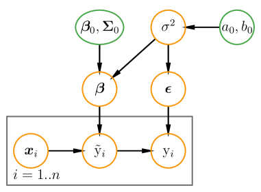
Equivalently, we can formulate the prior into one which is called the normal-inverse-Gamma (NIG) distribution:
Once again, by applying Bayes’ theorem “”, we obtain the posterior
where and
Let and . The posterior admits conjugacy and follows a NIG distribution:
Chapter 9 Problems \adftripleflourishright
-
1.
Suppose both and are probability density functions with
Show that for all .
-
2.
We have shown that the Gamma distribution is a conjugate prior for the precision parameter of a Gaussian distribution. Show that the inverse-Gamma distribution is a conjugate prior for the variance parameter of a Gaussian distribution with a fixed mean parameter.
- 3.
Chapter 10 Beyond Bayesian Approach: Gaussian Process Regression
10.1 Beyond Bayesian Approach: Gaussian Process Regression
IIn certain textbooks or college courses, discussions on the Gaussian process often occur without introducing the Bayesian linear model, leading to potential confusion. It will become evident that the Gaussian process regression truly “arises” from the Bayesian linear model with a zero-mean prior.
10.2 Predictive Distribution of Bayesian Linear Model with Zero-Mean Prior
Following from Bayesian linear model with a zero mean in Section 9.3 (p. 9.3), the predictive distribution for a new data point remains a Gaussian distribution:
| (10.1) | ||||
where the mean of the predictive distribution is the posterior mean of the weight parameter (i.e., ) multiplied by the new input, and the predictive variance is a quadratic form of the new input indicating that the predictive uncertainties grow with the magnitude of the new input.
However, this Bayesian linear model suffers from limited expressiveness, having problems in its ability to capture and represent complex relationships within the data. One solution to overcome this issue is to use a set of basis functions and transfer from the dimensional space to a higher-dimensional space, potentially capturing more complex relationships, say dimensional space: and . However, the introduction of basis functions comes with a computational challenge. Specifically, as the dimensionality grows, the computational complexity increases quadratically. For instance, the computation of the predictive variance changes from to . The quadratic growth in complexity can be a significant challenge, particularly when scalability and efficiency are important considerations.
Example 10.2.1 (Kernel Trick)
For some examples, we have:
-
1.
The computation of only has the dot product from the input space. So we could use kernel trick to do the computation. And each element is , where represents a kernel function. The computation of the kernel function is potentially less than .
-
2.
The computation of involves the dot product between the input space and the output space. So it cannot be reduced to the kernel form.
Having this in mind, if we can reduce the computation of Equation (10.1) involving the input space to having only dot products, we could apply the kernel trick. To achieve this, we transfer the parameters in Equation (10.1) to a high-dimensional space. This transformation from {} in -space to {} in -space yields the predictive distribution in the -space form:
where . Let and , we have
| (10.2) |
where we use the fact that . Note that we do not differentiate the notations of and in and -spaces. However, we only differentiate the notation of and in and -spaces, respectively. Next, by left-multiplying Equation (10.2) by and right-multiplying by , we transform the predictive distribution into inner product form:
where the input space only has the forms , and —adhering to the kernel trick requirement.
We define kernel variables as follows: , , and . Subsequently, we can express the predictive distribution in kernel form:
| (10.3) |
Since is positive definite (see Section 9.3, p. 9.3), it can be decomposed into . Therefore, it can be absorbed into the kernel function. For example, let , can be denoted by . Similarly, can be represented as , and as .
10.3 Kernels In A Nutshell
The kernel, employing basis functions, transforms to . This conversion changes the inner product from in the -dimensional space to in the -dimensional space. Consequently, the kernel matrix exhibits the following properties:
-
1.
should be symmetric, i.e., .
-
2.
The kernel matrix is positive semidefinite (PSD).
Proof [of Kernel Matrix is PSD] Let , . And for any vector , we have
This completes the proof.
We may find can be any function related to at first glance. However, due to the PSD property of the kernel matrix, this function is constrained to a specific form, ensuring that implicitly takes the shape of an inner-product in -dimensional space.
10.4 Gaussian Process from Zero-Mean Prior
We employ Gaussian processes (GPs) to characterize a distribution over functions. Gaussian processes are natural generalizations of multivariate Gaussian random variables to infinite (countably or continuous) index sets. Formally, we define Gaussian processes as follows:
Definition 10.1 (Gaussian Process)
A Gaussian process is a collection of random variables, any finite number of which have a joint Gaussian distribution. The definition does not exclude Gaussian processes with finite index sets, which would be simply Gaussian distributions.
10.4.1 Noise-Free Observations
Following the Bayesian linear model with zero-mean prior in Section 9.3 (p. 9.3), we assume a zero-mean prior and define for each input observation . Then, the mean and covariance for the prior output are:
| (10.4) | ||||
where the prior covariance matrix is specified manually and we could use a kernel function instead: .
Suppose we have the training input design matrix , training output vector , test input design matrix , and test output vector . We obtain the joint distribution of the training outputs and the test outputs by Equation (10.4):
Therefore, we could use Gaussian identities to obtain the marginal distribution of test outputs . Following from Section 9.3 (p. 9.3), assume a zero-mean prior and define . Given the observed training inputs , training outputs , and test inputs , the marginal distribution of test outputs is
Proof [of Lemma 10.4.1] Let and be jointly Gaussian random vectors:
Thus, it follows that
which completes the proof.
The marginal distribution of test outputs agrees with the kernel form of the Bayesian linear model with zero-mean prior in Equation (10.3), except that the noise term and the output are vectors now (i.e., ).
10.4.2 Noisy Observations
Following again from Section 9.3 (p. 9.3), we assume a zero-mean prior . And we define and . Then, the mean and covariance for the prior output are:
That is,
where is a Kronecker delta, which is equal to 1 if and only if and 0 otherwise. Therefore, we can obtain the joint distribution of the training outputs and the test outputs :
Similarly, we could use Gaussian identities to obtain the marginal distribution of test outputs .
The marginal distribution of test outputs aligns with the form of Equation (10.3), except that the output is a vector now (i.e., ).
10.4.3 Further Extension, Generalized Gaussian Process
Expanding upon the concept of the generalized linear model introduced in Section 7.1 (p. 7.1), we can assign distinct noise variance values to individual observations. Suppose the noise covariance matrix now is , where is a diagonal matrix. Then, the marginal distribution of test outputs becomes
Apparently, the noise covariance should not be dependent on the input matrix . Otherwise, we will not be able to use the kernel trick.
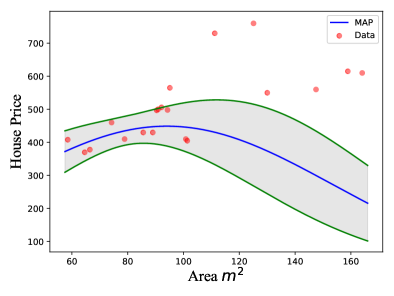
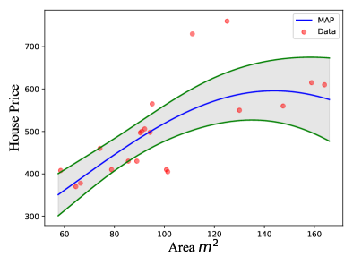
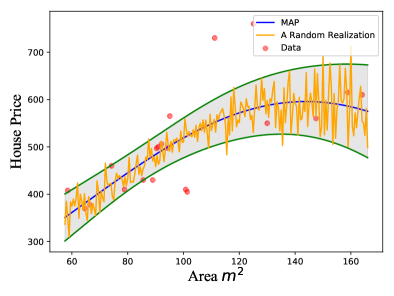
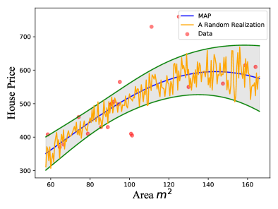
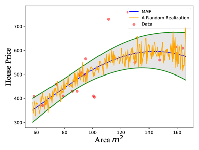
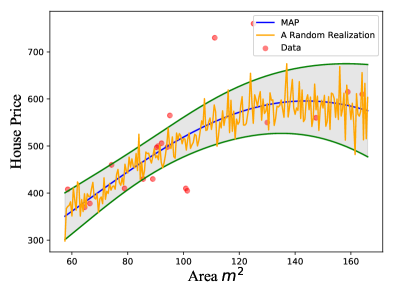
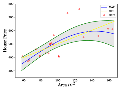
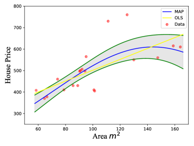
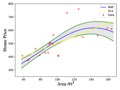
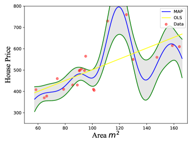
Example 10.4.1
For a data set where the inputs represents the house area and the output corresponds to the rent of the house. We use cross-validation (CV) to determine the parameters in the Gaussian kernel.
In Figure 10.1, the red dots represent the training inputs, the blue line signifies the MAP estimate via GP regressor, and the shaded area indicates the ones with a confidence interval of 95%.
In Figure 10.1(b), we employ the entire data set. While in Figure 10.1(a), we utilize only the data with house areas smaller than 100 . In this case, we can observe that the estimator in Figure 10.1(a) does not predict well when the house area is larger than 100 .
In Figure 10.2, we use the entire data set for prediction, and we draw four random realizations from the posterior as shown by orange lines. This offers a deeper understanding of the concept of distribution over functions.
In Figure 10.3, we repeat the data set once, twice, three times, and four times to investigate the impact of the number of data sets. The yellow line represents the predictor by OLS. It can be observed that the estimate from OLS remains constant since the data set is identical. To see this, suppose the OLS estimate for data without repeating is given by
The OLS estimate for data with repeating twice is given by
which is exactly the same as . Similarly, we can also show that the OLS estimate for data with repeating three times and four times are the same as well. This consistency also holds for different repetitions.
However, when we repeat the data set for the GP regressor, the estimator from the GP regressor exhibits a smaller variance when the data set size increases. In Section 9.2 (p. 9.2), we mentioned that the Bayesian model considers prior information on the parameters in the model, making it particularly useful to regularize regression problems where data information is limited. The size of data set is crucial in the Bayesian approach, as illustrated in Example 9.2.1 (p. 9.2.1). This example elucidates the Bayesian rationale underlying GP modeling.
10.5 Limitations of Gaussian Process from Non-Zero-Mean Prior*
When the prior mean is not zero (see Equation (9.2), p. 9.2), and the model is under the Gaussian noise , we transform the predictive distribution into
where we use the fact that if both and are nonsingular.
Following from Section 9.3 (p. 9.3), if we assume a non zero-mean prior and define , then, the mean and covariance for the prior output are:
Therefore, we could obtain the joint distribution of the training outputs and the test outputs by
By Gaussian identities, the marginal distribution of test outputs is
where we notice that we cannot find an explicit form in the -dimensional space for the mean of , precluding the application of the kernel trick in this context. Consequently, we encounter a limitation in flexibility when applying a non-zero-mean prior.
Chapter 10 Problems \adftripleflourishright
-
1.
Show that the linear kernel, polynomial kernel, and Gaussian kernel in Remark 10.3 exhibit the positive definite property.
Chapter 11 Proofs
A Dimension of Column Space and Row Space
In this appendix, we establish the equivalence stated in Lemma A, demonstrating that the dimension of the column space of a matrix is identical to the dimension of its row space. In other words, the row rank and the column rank of a matrix are equal. The dimension of the column space of a matrix is equal to the dimension of its row space, i.e., the row rank and the column rank of a matrix are equal.
Proof [of Lemma A] We first notice that the null space of is orthogonal complementary to the row space of : (where the row space of is equivalent to the column space of ). That is, vectors in the null space of are orthogonal to vectors in the row space of . To see this, suppose is the row partition of . For any vector , we have , that is, . And since the row space of is spanned by . Then, is perpendicular to any vectors from . This indicates .
Now, assuming the dimension of the row space of is , let be a set of vectors in p and form a basis for the row space. Consequently, the vectors are in the column space of ; furthermore, they are linearly independent. To see this, suppose we have a linear combination of the vectors: , that is, , and the vector is in null space of . But since is a basis for the row space of , is thus also in the row space of . We have shown that vectors from null space of is perpendicular to vectors from row space of , thus and . Then, are in the column space of and they are independent. This means that the dimension of the column space of is larger than . This result shows that row rank of column rank of .
If we apply this process again for . We will have column rank of row rank of . This completes the proof.
Further information can be drawn from this proof is that if is a set of vectors in p that forms a basis for the row space, then is a basis for the column space of . We formulate this finding into the following lemma.
B Cochran’s Theorem
In this appendix, we provide proof for Theorem 5.2.4 (p. 5.2.4). To prove the Cochran’s theorem, we need the following lemma.
Proof [of Lemma B] From (i) to (ii), by Lemma 2.7.1 (p. 2.7.1), the trace and rank of any idempotent matrix are the same. Then,
From (ii) to (iii), we have the following block Gaussian elimination for a block matrix (that is, matrix), where blocks are , respectively:
where blank entries indicate zeros. And
-
is used to add row-2, row-3, , row-(k+1) to row-1;
-
is used to add column-2, column-3, , column-(k+1) to column-1;
-
is used to subtract the row-2 by (row-1), subtract the row-3 by (row-1), ;
-
is used to subtract the column-2 by (column-1), subtract column-3 by (column-1), .
We notice that elementary operations/transformations will not change the rank of the matrix. Since is of rank , and in is of rank as well. We must have
which implies for all and .
From (iii) to (i). we have
This completes the proof.
Note on nomenclature.
The matrices are considered orthogonal if condition (iii) of Lemma B is met, and the rank is additive if condition (ii) is fulfilled.
We now prove the Cochran’s Theorem as follows.
Case 1.
If : From Lemma B, ’s are idempotent. By Spectral Theorem 2.7.1 (p. 2.7.1) and Lemma 2.7.1 (p. 2.7.1, the only possible eigenvalues of idempotent matrices are 0 and 1), we can rewrite the by , where is the spectral decomposition of . From the fact that rotations on the normal distribution do not change the distribution (Lemma 1.1, p. 1.1), we can define
Thus,
Case 2.
If , and : Let . Similarly, we can rewrite the by , where is the spectral decomposition of . From the fact that rotations on the normal distribution do not change the distribution, we can define
Thus,
Then, we decompose the into
Since we assume , and contains only 1 and 0 on the diagonal, we have . That is,
which implies . Thus, we have .
Case 3.
From Lemma B, if . Let and be the spectral decomposition of and , respectively. Then, we have
| (11.1) | ||||
Write out and :
Let and , we have
where the last equality is from Equation (11.1). This implies since and .
This completes the proof.
An alternative proof is presented in Gut (2009b). However, the author does not provide an inductive case for . Interesting readers can refer to it.
C Trace Trick for Quadratic Expectation of Random Variables
Proof [of Lemma C] For , we have
Thus, it follows that
where for any matrix , the trace trick is
if all , , and exist.
This completes the proof.
If we assume further that , then , where we usually engineer in real applications that .
D Famous Inequalities
In this section, we introduce some famous inequalities that will be often used. When considering random matrices, the Cauchy–Schwarz inequality is considered one of the most important and widely used inequalities in mathematics. For any random matrices and , we have where the inner product is defined as .
The result can be applied to non-random matrices and vectors. For any matrices and , we have This is a special form of the Cauchy-Schwarz inequality, where the inner product is defined as . Similarly, for any vectors , we have (11.2) In two-dimensional case, it becomes The vector form of the Cauchy-Schwarz inequality plays a crucial role in various branches of modern mathematics, including Hilbert space theory and numerical analysis (Wu and Wu, 2009). Here, we present the proof for the vector form of the Cauchy-Schwarz inequality for simplicity. To see this, given two vectors , we have
from which the result follows. The equality holds if and only if for some constant , i.e., and are linearly dependent.
Proof [of Lemma D] We notice the trick that since x is nonnegative. This implies . We also have
This completes the proof.
The Chebyshev’s inequality can be easily verified by defining (which is non-negative) and applying Markov’s inequality to y.
E Taylor’s Expansion
The Taylor’s expansion, or also known as the Taylor’s series, approximates the function around the value of by a polynomial in a single indeterminate . To see where this series comes from, we recall from the elementary calculus course that the approximated function around for is given by
That is, the is approximated by a polynomial with a degree of 2. Suppose we want to approximate by the more general polynomial with a degree of 2 by . An intuitive idea is to match the gradients around the point. That is,
This makes and agrees with our claim that around the 0 point. We shall not give the details of the proof.
Chapter 12 Matrix Decomposition
A CR Decomposition
The CR decomposition, as introduced in Strang (2021); Strang and Moler (2022), is presented as follows. Subsequently, we delve into the examination of its existence and the underlying origin in the subsequent sections. Any rank- matrix admits the following decomposition: where contains the first linearly independent columns of , and is an matrix used to reconstruct the columns of from the columns of . In particular, is the reduced row echelon form (RREF) of without the zero rows. This decomposition leads to a potential reduction or increase in storage requirements, transitioning from floating-point numbers to floating-point numbers.
A.1 Existence of the CR Decomposition
Since matrix is of rank , it possesses linearly independent columns. We proceed by selecting linearly independent columns from and assembling them into matrix :
Upon acquiring the linearly independent columns from matrix , we can establish the existence of the CR decomposition through the column space perspective of matrix multiplication.
Column space view of matrix multiplication.
The multiplication of two matrices, and , is , i.e., each column of is a linear combination of columns from .
Proof [of Theorem A] Since the rank of matrix is and contains linearly independent columns from , the column space of is equivalent to the column space of . For any additional column in , can be represented as a linear combination of the columns of , i.e., there exists a vector such that , . By assembling these ’s into the columns of matrix , we obtain
from which the result follows.
A.2 Reduced Row Echelon Form (RREF)
We perform Gaussian elimination on a square matrix, where denotes a value that is not necessarily zero, and boldface indicates the value has just been changed:
Furthermore, Gaussian elimination is applicable to rectangular matrices. Here, we provide an example for a matrix:
where the blue-highlighted numbers represent pivots. The final matrix obtained above is termed the row echelon form. It is worth noting that, in this specific example, the 4-th row becomes a zero row. Going further, we perform row operations, subtracting multiples of the subsequent row to zero out the entries above the pivots:
where subtracts twice the -nd row from the -st row, and adds the -rd row to the -st row and subtracts twice the -rd row from the -nd row. Finally, we obtain the full reduced row echelon form by making the pivots to be 1:
where makes the pivots to be 1. We call this final matrix the reduced row echelon form of , where it has 1’s as pivots and zeros above the pivots.
Proof [Informal Proof of Lemma A.2 and Lemma A.2] Following the Gaussian elimination steps, the count of pivot elements corresponds to the number of linearly independent columns in matrix , which, in turn, is precisely the rank of the matrix.
Using the example above, we express as
Observing that the columns 1, 3, 4 of have only one element 1, we construct a matrix (identical to the column matrix in CR decomposition), whose first three columns are the same as the 1-st, 3-rd, 4-th columns of matrix , denoted as . Furthermore, since the last row of is a zero vector, the 4-th column of doesn’t contribute to any computation, allowing us to disregard both the 4-th column of and the 4-th row of . Thus, this is the only matrix that can reconstruct the 1-st, 3-rd, 4-th columns of , as the pivots of are all 1. We obtain
This completes the proof.
In short, we first compute the reduced row echelon form of the matrix by . Subsequently, is derived by eliminating the non-pivot columns from (identified by columns in lacking pivots). And is obtained by eliminating zero rows from . And this is actually a special case of rank decomposition (Theorem A.3) of matrix . However, CR decomposition is so special that it involves the reduced row echelon form so we introduce it here particularly.
possesses a distinctive structure where its columns, housing the pivots, form an identity matrix. Note again that we can just remove the zero rows from the reduced row echelon form to obtain this matrix . In Strang (2021), the authors give a specific notation for the reduced row echelon form without removing the zero rows as :
where the permutation matrix puts the columns of identity matrix into the correct positions, matching the first linearly independent columns of the original matrix .
The fundamental theorem in linear algebra, stating that the row rank equals the column rank of any matrix, can be demonstrated through the UTV framework (Theorem A, p. A, see Lu (2021a) for using UTV to prove the theorem). The CR decomposition also provides insight into this theorem.
Proof [of Theorem A, p. A, An Alternative Approach] For CR decomposition of matrix , we have , where is a permutation arranging the columns of the identity matrix into the correct positions as shown above. It can be easily verified that the rows of are linearly independent due to the nonsingularity of the submatrix , implying that the row rank of is .
Firstly, from the definition of the CR decomposition, the columns of are from linearly independent columns of , and the column rank of is . Further,
-
Since , all rows of are linear combinations of the rows of . That is, the row rank of is no larger than the row rank of ;
-
From , we also have . That is, . is nonsingular since it has full column rank . Then, all rows of are also linear combinations of the rows of . That is, the row rank of is no greater than the row rank of ;
-
By “sandwiching,” the row rank of is equal to the row rank of , which is .
Therefore, both the row rank and column rank of are equal to . This completes the proof.
A.3 Rank Decomposition
As previously mentioned, the CR decomposition represents a particular instance of rank decomposition. To provide a rigorous demonstration of the existence of rank decomposition, we present the following theorem.
Proof [of Theorem A.3] By ULV decomposition in Theorem 2.5 (p. 2.5), we can decompose by
Let and , i.e., contains only the first columns of , and contains only the first rows of . Then, we still have , where and . This is also known as the reduced ULV decomposition, as shown in Figure 2.6 (p. 2.6). Let { and }, or { and }, we find such rank decompositions.
The rank decomposition is not unique. Even by elementary transformations, we have
where represent elementary row and column operations, and . The transformation is rather general, and there are dozens of these , , and . By similar construction on this decomposition as shown in the proof above, we can recover another rank decomposition.
Similarly, one can obtain matrices and through methods such as SVD, URV, CR, CUR, and various other decomposition algorithms. However, we may connect the different rank decompositions by the following lemma. For any two rank decompositions of , there exists a nonsingular matrix such that
Proof [of Lemma A.3]
Since , we have . It is evident that such that is a square matrix with full rank and thus is nonsingular. This implies . Let , we have and .
B QR Decomposition
In this appendix, we provide the proof for Theorem 2.4 (p. 2.4), the existence of QR decomposition. In many applications, we are interested in the column space of a matrix . The successive spaces spanned by the columns of are
where is the subspace spanned by the vectors included in the brackets. The idea of QR decomposition is the construction of a sequence of orthonormal vectors that span the same successive subspaces. That is,
To achieve this, we first discuss how to project a vector onto another vector, based on which the Gram-Schmidt process is employed iteratively.
B.1 Project a Vector Onto Another Vector
Projecting a vector onto another vector involves determining the vector on the line of that is closest to . The resulting projection vector, denoted as , is a scalar multiple of . Let , then is perpendicular to , as shown in Figure 12.1(a). This leads to the following outcome:
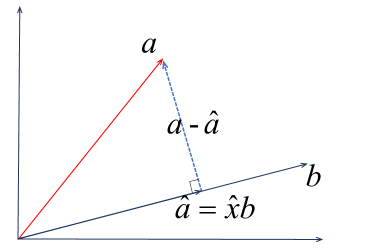
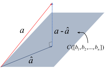
B.2 Project a Vector Onto a Plane
Projecting a vector onto a space spanned by involves determining the vector closest to within the column space of . The resulting projection vector, denoted as , is expressed as a linear combination of : . This scenario can be formulated as a least squares problem, wherein the normal equation is solved, where and . For each vector , the projection of in the direction of can be similarly obtained by
Let , this results in
i.e., is perpendicular to the column space of , as shown in Figure 12.1(b).
B.3 Existence of the QR Decomposition via the Gram-Schmidt Process
We proceed by establishing the Gram-Schmidt process through vector projection. Given three independent vectors and the space spanned by the three vectors, denoted as , i.e., the column space of matrix . We intend to construct three orthogonal vectors such that = . We then normalize these orthogonal vectors by dividing each by its length, resulting in three orthonormal vectors: , , and .
For the first vector, we directly set . The second vector, , must be perpendicular to the first. This is achieved by considering the vector and subtracting its projection along :
where the first equation shows that is a multiplication of a matrix and , i.e., project onto the orthogonal complement space of . The second equation shows that is a linear combination of and . Clearly, the space spanned by and is the same space spanned by and . The situation is shown in Figure 12.2(a), in which we choose the direction of as the -axis in the Cartesian coordinate system. is the projection of onto the line . It can be clearly shown that the part of perpendicular to is from the figure.
For the third vector , it must be perpendicular to both the and , which is actually the vector subtracting its projection along the plane spanned by and :
| (12.1) | |||||
where the first equation shows that is a multiplication of a matrix and , i.e., project onto the orthogonal complement space of . The second equation shows that is a linear combination of , , and . We will see this property is essential in the idea of QR decomposition. Again, it can be shown that the space spanned by is the same space spanned by . The situation is shown in Figure 12.2(b), in which we choose the direction of as the -axis of the Cartesian coordinate system. is the projection of onto the line , and is the projection of onto the line . It can be shown that the part of perpendicular to both and is from the figure.
Finally, we normalize each vector by dividing its length, resulting in three orthonormal vectors: , , and .
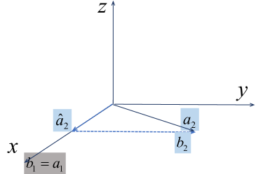
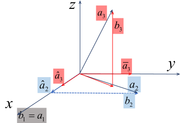
This idea can be extended to a set of vectors rather than only three. And we refer to this process as the Gram-Schmidt process. After this process, matrix will be triangularized. The method is named after Jørgen Pedersen Gram and Erhard Schmidt, but it appeared earlier in the work of Pierre-Simon Laplace in the theory of Lie group decomposition.
The Gram–Schmidt process is not the sole algorithm for obtaining the QR decomposition. There are several other QR decomposition algorithms available, such as Householder reflections and Givens rotations, which exhibit greater robustness in the presence of round-off errors. These QR decomposition methods may also alter the order in which the columns of are processed.
B.4 Orthogonal vs Orthonormal
The vectors are mutually orthogonal when their dot products are zero whenever . When each vector is divided by its length, the vectors become orthogonal unit vectors. Then the vectors are called mutually orthonormal. We usually put the orthonormal vectors into a matrix .
When : the matrix is easy to work with because .
When : the matrix is square, means that , i.e., the transpose of is the inverse of . Then we also have , i.e., is the two-sided inverse of . We call this an orthogonal matrix. Note here we use the term orthogonal matrix to mean the matrix has orthonormal columns. The term orthonormal matrix is not used for historical reasons.
B.5 Property of the QR Decomposition
For any matrix , we have the property: is the orthogonal complement of the column space in n: ; This relationship is known as the rank-nullity theorem, and its proof can be found in Theorem 2.3.1 (p. 2.3.1). Specifically, QR decomposition yields a basis for this subspace. In singular value decomposition, we will also find the basis for and .
Proof [of Lemma B.5]
From the Gram-Schmidt process, it is trivial that is equal to for all . Thus, , and is an orthonormal basis for the column space of .
Additionally, we have , and .
Since the space spanned by is also perpendicular with dimension , thus, is an orthonormal basis for .
B.6 Uniqueness of the QR Decomposition
The results of the QR decomposition from the Gram-Schmidt process, the Householder algorithm, and the Givens algorithms are different (see Lu (2021a)). Thus, from this point, QR decomposition is not unique.
Example 12.1 (Non-Uniqueness of the QR Decomposition)
Suppose the matrix is given by
The QR decomposition of can be obtained by
Thus, the QR decomposition of is not unique.
However, the uniqueness of the reduced QR decomposition for full column rank matrix is guaranteed when has positive diagonals as shown in the “main proof” of Section B.3 by inductive analysis. We here provide an alternative proof for the uniqueness of the reduced QR decomposition if the diagonal values of are positive. Suppose matrix is an matrix with full column rank and . Then, the reduced QR decomposition is unique if the main diagonal values of are positive.
Proof [of Corollary B.6] Suppose the reduced QR decomposition is not unique, we can complete it into a full QR decomposition, then we can find two such full decompositions satisfying . This implies , where is an orthogonal matrix. Write out the equation, we have
This implies
Since contains mutually orthonormal columns, and the first column of is of norm 1. Thus, . We notice that and for by assumption such that and , implying that can only be positive 1. Since is an orthogonal matrix, we also have
Applying this process to the submatrices of , , and , we will find the upper-left submatrix of is an identity: such that . This implies and leads to a contradiction. And thus the reduced QR decomposition is unique.
We complete the proof.
C Schur Decomposition
Schur decomposition for symmetric matrices.
When dealing with a symmetric matrix , we find that . Consequently, is a diagonal matrix. And this diagonal matrix actually contains the eigenvalues of . All the columns of are eigenvectors of . This leads us to the conclusion that symmetric matrices are inherently diagonalizable, even in the presence of repeated eigenvalues.
Moreover, the matrix and are in the notion of similar matrices. {dBox}
Definition 12.1 (Similar Matrices)
For any nonsingular matrix , the matrices and are called similar matrices.
Proof [of Lemma C] For any eigenpair of , we have . Consequently, , demonstrating that is an eigenvector of associated with .
Similarly, for any eigenpair of , we have . Then, , indicating that is an eigenvector of corresponding to .
Regarding the the trace of , we can establish that , where the first equality comes from the fact that the trace of a product is invariant under cyclical permutations of the factors:
if all , , and exist.
Regarding the rank of , we separate it into two claims as follows.
Rank claim 1: if is nonsingular.
We will begin by demonstrating that if is nonsingular. Consider any vector in the null space of , that is, . Consequently, , that is, also resides in the null space of . This, in turn, implies .
Conversely, for any vector in the null space of , i.e., , we can deduce that . That is, is also in the null space of . And this indicates .
By applying the concept of “sandwiching,” the two arguments presented above lead to the following conclusion:
Rank claim 2: if is nonsingular.
We observe that the row rank of a matrix is equivalent to its column rank (Corollary A, p. A). Therefore, . Since is nonsingular, as per claim 1, we can conclude that , where the last equality is again from the fact that the row rank is equal to the column rank for any matrix. This establishes that , as claimed.
Since and are nonsingular, we can conclude that , where the first equality is from claim 1, and the second equality is from claim 2. We complete the proof.
C.1 Existence of the Schur Decomposition
To prove Theorem C, we need to use the following lemmas. We have the following properties for determinant of matrices: The determinant of the product of two matrices is ; The determinant of the transpose is ; Suppose matrix has an eigenvalue , then ; Determinant of any identity matrix is ; Determinant of an orthogonal matrix : Given any square matrix and orthogonal matrix , we have Suppose , then .
Proof [of Lemma C.1] Let . We have and
For any eigenvalue , by Lemma C.1, we have
where the last equality is from the fact that if matrix has a block formulation: , then .
Since is an eigenvalue of and , then means is also an eigenvalue of .
We then prove the existence of the Schur decomposition by induction.
Proof [of Theorem C: Existence of Schur Decomposition] We note that the theorem is trivial when by setting and . Suppose the theorem is true when for some . If we prove the theorem is also true when , then we complete the proof.
Suppose for , the theorem is true for .
Suppose further contains orthogonal vectors as constructed in Lemma C.1, where is an eigenvector of corresponding to eigenvalue , and its norm is 1; and are orthonormal to . Let the other eigenvalues of be . Since we assume the theorem is true for , we can find a matrix with eigenvalues . So we have the following property by Lemma C.1:
Let Then, it follows that
| (By the assumption for ) | ||||
| () | ||||
We then have , where is an upper triangular matrix, and is an orthogonal matrix since and
are both orthogonal matrices.
This completes the proof.
C.2 Other Forms of the Schur Decomposition
From the proof of the Schur decomposition, we obtain the upper triangular matrix by appending the eigenvalue to . From this process, the values on the diagonal are always eigenvalues. Therefore, we can decompose the upper triangular into two parts.
A strictly upper triangular matrix is an upper triangular matrix having 0’s along the diagonal as well as the lower portion. Another proof for this decomposition is that and (where ) are similar matrices so that they have the same eigenvalues (Lemma C). And the eigenvalues of any upper triangular matrices are on the diagonal. To see this, for any upper triangular matrix , where the diagonal values are for all , we have
where is the -th basis vector in n. So we can decompose into and .
D Spectral Decomposition (Theorem)
In this section, we provide the proof for Theorem 2.7.1 (p. 2.7.1), the existence of spectral decomposition. We prove the theorem in several steps.
Proof [of Lemma D] Suppose eigenvalue is a complex number , where and are real. Its complex conjugate is . Same for complex eigenvector and its complex conjugate , where and are real vectors. We then have the following property:
We take the dot product of the first equation with and the last equation with :
Then we have the equality . Since is a real number, the imaginary part of is zero and is real.
Proof [of Lemma D] Suppose eigenvalues and correspond to eigenvectors and , respectively, such that and . We have the following equality:
and
which implies . Since eigenvalues , the eigenvectors are orthogonal.
For any matrix multiplication, we have the rank of the multiplication result no larger than the rank of the inputs. However, the symmetric matrix is rather special in that the rank of is equal to that of which will be used in the proof of singular value decomposition in the next section. For any matrix , , then the matrix multiplication has ()min((), ()).
Proof [of Lemma D] For matrix multiplication , we have
-
All rows of are combination of the rows of , the row space of is a subset of the row space of . Thus ()().
-
All columns of are combination of columns of , the column space of is a subset of the column space of . Thus ()().
Therefore we have, ()min((), ()).
For the third property of symmetric matrix, we need the definition of similar matrices and the property about eigenvalues of similar matrices (see Lemma C, p. C).
Proof [of Lemma D] We note that there is at least one eigenvector corresponding to . And for such eigenvector , we can always find additional orthonormal vectors so that forms an orthonormal basis in n. Put the into matrix and into matrix :
We then have
As a result, and are similar matrices such that they have the same eigenvalues since is nonsingular (even orthogonal here, see Lemma C, p. C). We obtain
If has multiplicity , then the term occurs times in the polynomial from the determinant , i.e., the term occurs times in the polynomial from . In other words, and is an eigenvalue of .
Let . Since , the null space of is not none. Suppose , i.e., and is an eigenvector of .
From we have , where is any scalar. From the left side of this equation, we have
| (12.2) | ||||
And from the right side of the equation, we have
| (12.3) | ||||
Combining Equation (12.3) and Equation (12.2), we obtain
which means is an eigenvector of corresponding to the eigenvalue (the same eigenvalue corresponding to ). Since is a combination of , which are orthonormal to , the can be chosen to be orthonormal to .
To conclude, if we have one eigenvector corresponding to whose multiplicity is , we could construct the second eigenvector by choosing one vector from the null space of constructed above. Suppose now, we have constructed the second eigenvector , which is orthonormal to . For such eigenvectors and , we can always find additional orthonormal vectors so that forms an orthonormal basis in n. Put the into matrix and into matrix :
We then have
where such that . If the multiplicity of is , and the null space of is not none so that we can still find a vector from the null space of and . Now we can construct a vector , where and are any scalar values, such that
Similarly, from the left side of the above equation we will get . From the right side of the above equation we will get . As a result,
where is an eigenvector of and is orthogonal to and . And it is easy to construct the eigenvector to be orthonormal to the first two.
The process can go on, and finally, we will find orthonormal eigenvectors corresponding to .
Actually, the dimension of the null space of is equal to the multiplicity . It also follows that if the multiplicity of is , there cannot be more than orthogonal eigenvectors corresponding to . Otherwise, it will lead to the contradiction that we could find more than orthogonal eigenvectors.
The proof of the Spectral Theorem 2.7.1 (p. 2.7.1) is evident from the lemmas above. Also, we can use Schur decomposition to prove the existence of spectral decomposition (see Theorem C, p. C).
Proof [of Lemma D] For any symmetric matrix , we have , in spectral form, as and also . Since we have shown in Lemma D that the rank of the matrix multiplication ()min((), ()). Therefore, we have
-
From , we have ;
-
From , we have ,
The inequalities above give us a contradiction. And thus , which is the total number of nonzero eigenvalues.
Since is nonsingular if and only if all of its eigenvalues are nonzero, has full rank if and only if is nonsingular.
E Singular Value Decomposition (SVD)
If we append additional silent columns that are orthonormal to the eigenvectors of , just like the silent columns in QR decomposition, we will have an orthogonal matrix . A similar procedure applies to the columns of . We then illustrate the full SVD for matrices in Theorem 2.6 (p. 2.6), where we formulate the difference between reduced and full SVD in the blue text. The comparison of reduced and full SVD is shown in Figure 2.8 (p. 2.8), where white entries are zero, and blue entries are not necessarily zero.
E.1 Existence of the SVD
To prove the existence of the SVD, we need to use the following lemmas. We may notice that the singular values are the square roots of the eigenvalues of . While, negative values do not have square roots such that its eigenvalues must be nonnegative. For any matrix , has nonnegative eigenvalues.
Proof [of Lemma E.1] Given an eigenvalue and its corresponding eigenvector and of , we have
Since and . It then follows that .
Since has nonnegative eigenvalues, we then can define the singular value of such that is the eigenvalue of , i.e., . This is essential for establishing the existence of SVD.
We have shown in Lemma D (p. D) that ()min((), ()). However, the symmetric matrix is rather special in that the rank of is equal to . And the proof is provided in Lemma 2.2 (p. 2.2).
In the form of SVD, we claimed the matrix is a sum of rank-one matrices, where is the number of nonzero singular values. And the number of nonzero singular values is actually equal to the rank of the matrix.
Proof [of Lemma E.1]
The rank of any symmetric matrix (here ) equals the number of nonzero eigenvalues (with repetitions) by Lemma D (p. D). So the number of nonzero singular values equals the rank of . By Lemma 2.2 (p. 2.2), and have the same rank, so the number of nonzero singular values equals the rank of .
We are now ready to prove the existence of SVD.
Proof [of Theorem E: Existence of SVD] Since is a symmetric matrix, by Spectral Theorem 2.7.1 (p. 2.7.1) and Lemma E.1 (p. E.1), there exists an orthogonal matrix such that
where is a diagonal matrix containing the singular values of , i.e., contains the eigenvalues of . Specifically, and are the nonzero eigenvalues of with being the rank of . I.e., are the singular values of . In this case, . We are now in the central part of the proof. Start from , , i.e., the eigenvector of corresponding to : 1. Multiply both sides by : 2. Multiply both sides by : where we notice this form can find the eigenvector of corresponding to , and the eigenvector is . Since the length of is , we then define with norm 1. These ’s are orthogonal because . That is,
Since , we have
which completes the proof.
By appending silent columns into and , we can easily find the full SVD.
E.2 Property of the SVD
For any matrix, we have the following property:
-
is the orthogonal complement of the row space in p: ;
-
is the orthogonal complement of the column space in n: ;
This is called the fundamental theorem of linear algebra and is also known as the rank-nullity theorem (Theorem 2.3.1, p. 2.3.1). In specific, from SVD, we can find an orthonormal basis for each subspace (see Lemma 2.6, p. 2.6).
Proof [of Lemma 2.6] From Lemma D (p. D), for symmetric matrix , is spanned by the eigenvectors, thus is an orthonormal basis of .
Since,
-
1.
is symmetric, then the row space of equals the column space of .
-
2.
All rows of are linear combinations of rows of , so the row space of row space of , i.e., .
-
3.
The row space of = the column space of = the row space of , i.e., . Thus, is an orthonormal basis of .
Further, the space spanned by is an orthogonal complement to the space spanned by , so is an orthonormal basis of .
If we apply this process to , we will prove the rest claims in the lemma.
Alternatively, we can see that is a basis for the column space of by Lemma A (p. A) 333As a recap, for any matrix , let be a set of vectors in p, which forms a basis for the row space, then is a basis for the column space of ., since .
Chapter 13 Pseudo-Inverse
If the matrix is nonsingular, the solution to the linear system can be straightforwardly obtained by taking the inverse of , yielding . In cases where is not square or is singular, the inverse does not exist. Nevertheless, we can still determine its pseudo-inverse, represented as a matrix denoted by . Before delving into the discussion on pseudo-inverse, we introduce concepts such as one-sided inverse, generalized inverse, and reflexive generalized inverse. However, readers have the option to skip these sections while still grasping the overall concept of pseudo-inverse.
A One-Sided Inverse
We first provide the rigorous definition of the one-sided inverse. {dBox}
Definition 13.1 (One-Sided Inverse)
For any matrix , a matrix is considered a left inverse of if it satisfies the condition:
In such cases, is termed left-invertible. Similarly, a matrix is called a right inverse of if the following holds:
In this scenario, is denoted as right-invertible.
A word on the notation: The superscript in and signifies the one-sided inverse of and should not be interpreted as the inverse of or .
Proof [of Lemma A] If has full column rank, then the matrix attains full rank (see Lemma 2.2, p. 2.2). Therefore, . This implies that acts as a left inverse of .
Conversely, suppose is left-invertible with . Since all rows of are combinations of the rows of , meaning the row space of is a subset of the row space of . We then have , indicating , and has full column rank.
Similarly, we can show is right-invertible if and only if has full row rank, and acts as a right inverse of .
In the proof above, we established that serves as a specific left inverse for when it possesses full column rank. Similarly, acts as a specific right inverse for when it has full row rank. However, obtaining the inverse of a nonsingular matrix involves a complex process, requiring floating-point operations (flops) (Lu, 2021a). In our scenario, finding the inverses of and demands and flops, respectively. A more straightforward approach to acquire a one-sided inverse involves elementary operations.
Assuming has full column rank, we can apply row elementary operations to such that
| (13.1) |
where , is an identity matrix, is a identity matrix, and is an matrix. Then, it can be easily verified that , establishing as a left inverse of .
Similarly, consider with full row rank. By applying column elementary operations to , we obtain
| (13.2) |
where is a matrix. Then, is a right inverse of .
More generally, the following two propositions provide the methods for discovering more left inverses or right inverses of a matrix. Suppose is left-invertible (). Then, is a left inverse of , where can be any matrix, and is the row elementary transformation of such that is invertible (since has full column rank ) and . We can verify that in Equation (13.1) is a specific left inverse of by setting . Since , , and , we have
where the last equality is from the assumption that .
Similarly, we can verify that in Equation (13.2) is a specific right inverse of by setting . Since , , and , we have
where again the last equality is from the assumption that .
Under specific conditions, the linear system has a unique solution. Suppose is left-invertible (), and is the left inverse of . Then, the linear system has a unique solution if and only if And the unique solution is given by
Proof [of Proposition A] Suppose is the solution of , then
That implies and . For the reverse, suppose , and let . Substituting into , we have
which implies is a solution of if .
To prove the uniqueness, suppose and are two solutions of . We have , hence . Since is left-invertible so that has full column rank , the dimension of the row space of is as well such that the null space of is of dimension 0 (i.e., by the fundamental theorem of linear algebra, see Theorem 2.3.1, p. 2.3.1). Therefore, , which completes the proof.
In the fundamental theorem of linear algebra (Figure 2.2, p. 2.2), if is left-invertible, its row space spans the entire p (indicating has full column rank ). The condition implies that is in the column space of such that has at least one solution, and the above proposition shows that this solution is unique.
Proof [of Proposition A] It is straightforward to verify that
so that is a solution of .
We notice that if is right-invertible, then it has full row rank . In the fundamental theorem of linear algebra (Figure 2.2, p. 2.2), the column space of spans the entire space of n if is right-invertible. Then, any vector is in the column space of such that has at least one solution.
B Generalized Inverse (g-inverse)
We mentioned previously that if the matrix is nonsingular, the linear system can be easily solved using the inverse of , resulting in . However, for an matrix , the inverse does not exist if is neither square nor nonsingular. Nevertheless, when lies in the column space of , we can still determine the solution to the linear system. The association between the solution and the target vector is expressed by the generalized inverse of : . {dBox}
Definition 13.2 (Generalized Inverse)
Suppose matrix has rank with . Then, a generalized inverse of is a matrix that satisfies
or equivalently,
for any .
To demonstrate the equivalence between and , that is, we want to show satisfies if and only if it satisfies . For any , a exists such that . If and satisfy , then
indicating that and also satisfy . Conversely, suppose and satisfy , then
which implies and also satisfy .
Multiply on the left of by and utilize the definition of the projection matrix in Definition 2.2 (p. 2.2), we obtain such that is idempotent, which implies is a projection matrix (not necessarily an orthogonal projection). For any matrix and its generalized inverse , is a projection matrix but not necessarily an orthogonal projection. Same claim can be applied to as well.
Proof [of Lemma B] From , we notice that . Moreover,
where the first inequality comes from the fact that the columns of are combinations of columns of , and the second inequality comes from the fact that the rows of are combinations of rows of .
For the second part, we have
where the first inequality is from the fact that the columns of are combinations of the columns of , and the second inequality is from the fact that the columns of are combinations of the columns of . From again, , which implies by “sandwiching” that
Similarly, we also have
where the first inequality is from the fact that the rows of are combinations of the rows of , and the second inequality is from the fact that the rows of are combinations of the rows of . By “sandwiching” again, we have
which completes the proof.
In Lemma A, we demonstrated that the left inverse exists if and only if has full column rank, and the right inverse exists if and only if has full row rank. However, this is not required in the generalized inverse. When this full rank condition is satisfied, we have the following property. Given any matrix and its generalized inverse , then we have 1. has full column rank if and only if ; 2. has full row rank if and only if .
Proof [of Lemma B] For (1). suppose has full column rank, and we have shown in Lemma B that . Thus, , and is nonsingular. We have
For the reverse implication, suppose , which implies . From , we have such that has full column rank.
Similarly, we can show has full row rank if and only if .
Suppose now that is any generalized inverse of , and define . Recall that , we have
which implies can be constructed for any generalized inverse .
Proof [of Lemma B] For (1), from , , we have such that is a generalized inverse of .
For (2), it can be easily verified that such that is a generalized inverse of for any .
For (3), we realize that , which implies is a generalized inverse of .
C Reflexive Generalized Inverse (rg-inverse)
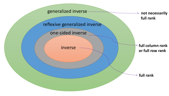
Definition 13.3 (Reflexive Generalized Inverse)
Suppose matrix has rank with . Then, a reflexive generalized inverse of is a matrix that satisfies the conditions:
and
That is, is a g-inverse of , and is a g-inverse of .
Suppose matrix is of rank . It can be factored as , where and are elementary transformations on . Then, we can construct such a reflexive generalized inverse of as
where , can be any matrix so that the reflexive generalized inverse is not unique. This construction of the reflexive generalized inverse also shows that the reflexive generalized inverse exists for any matrix . Thus, the reflexive generalized inverse is a more general inverse of compared to the one-sided inverse which may not exist. For any matrix , and and are two generalized inverses of , then is a reflexive generalized inverse of . It can be easily verified that and for the lemma above.
Proof [of Lemma C] Firstly, we establish the result: Since the columns of are combinations of the columns of , we have . In Lemma 2.2 (p. 2.2), we prove that . This implies and . Furthermore, the orthogonal complement of is , and the orthogonal complement of is . Therefore, by fundamental theorem of linear algebra in Theorem 2.3.1 (p. 2.3.1), we have Then there exists a set of vectors such that the -th column of can be expressed as . In matrix form, with , we have
Then,
By condition of g-inverse, we have for any . This implies and
| (13.4) |
Now, let’s examine :
The same argument applies to . Thus,
| (13.5) |
Combining Equation (13.4) and Equation (13.5), we conclude that is a reflexive generalized inverse of . Similarly, we can show is a reflexive generalized inverse of as well.
From the definition, it is evident that a reflexive generalized inverse is a specialized form of a generalized inverse. Under specific conditions, these two types of inverses are equivalent.
Proof [of Lemma C] Suppose is a generalized inverse of , then . Suppose further, is also a reflexive generalized inverse, then . We have
where the two inequalities are from Lemma B. This implies .
For the reverse, suppose is a generalized inverse of , then . And suppose further that , we have
where the first inequality is from the fact that the rows of are combinations of the rows of , and the second inequality is from the fact that the columns of are combinations of the columns of . This implies and . Then, there exists a set of vectors such that the column- of can be expressed as . That is, for , we have
We realize again that , then
where the last equality is form condition ; and thus, is a generalized inverse of . From Lemma C, is a reflexive generalized inverse of , which completes the proof.
Concluding this section, we provide insights into the rank of matrices in reflexive generalized inverses. Consider a matrix and its generalized inverse . Utilizing the result in Lemma C and the result from the rank of g-inverses in Lemma B, we have
D Pseudo-Inverse
As previously mentioned, for a matrix , we can find its pseudo-inverse, a matrix denoted by . In words, when multiplies a vector in its row space, this produces in the column space (see Figure 2.2 p. 2.2). Those two spaces have equal dimension , i.e., the rank. is always invertible when restricted to these spaces, and inverts . That is, when is in the row space of . And when is in the column space of (see Figure 13.2).
The null space of coincides with the null space of . It contains the vectors in n with . Those vectors are perpendicular to every in the column space. We delay the proof of this property in Lemma D.
More formally, the pseudo-inverse, or also known as Moore-Penrose pseudo-inverse, , is defined by the unique matrix satisfying the following four criteria:
| (13.6) |
In Lemma B, we claimed that and are idempotent if is a g-inverse of , and thus they are both projection matrices (Definition 2.2, p. 2.2). Since is the pseudo-inverse of 111We speak of “the pseudo-inverse” rather than “a pseudo-inverse” since the pseudo-inverse is unique as we will prove shortly., by conditions, they are symmetric such that they are orthogonal projection matrices as well (Lemma 2.7.2, p. 2.7.2).
The existence of a pseudo-inverse for any matrix is further supported by the pseudo-inverse obtained from the CR decomposition of the matrix. Every matrix has a pseudo-inverse.
Proof [of Lemma D] Given the CR decomposition (Theorem A, p. A) of , let
where and . 222It can be easily checked that is the pseudo-inverse of and is the pseudo-inverse of . Notably, and are invertible since and have full rank from the property of the CR decomposition.
Then, we can check that
This implies is the pseudo-inverse of and the existence of the pseudo-inverse.
Proof [of Lemma D] Suppose and are two pseudo-inverses of . Then
which implies the uniqueness of pseudo-inverse.
We are now ready to show the four subspaces in the pseudo-inverse. Given the pseudo-inverse of , we have the following properties: The column space of is the same as the row space of ; The row space of is the same as the column space of ; The null space of is the same as the null space of ; The null space of is the same as the null space of . The relationship of the four subspaces is shown in Figure 13.2.
Proof [of Lemma D] Since is a special rg-inverse, by Lemma C, we have
By and of the definition of pseudo-inverses, we also have
Utilizing the fundamental theorem of linear algebra (Theorem 2.3.1, p. 2.3.1), we realize that is the orthogonal complement to , and is the orthogonal complement to :
This implies
That is, and . According to the fundamental theorem of linear algebra, this also implies and .
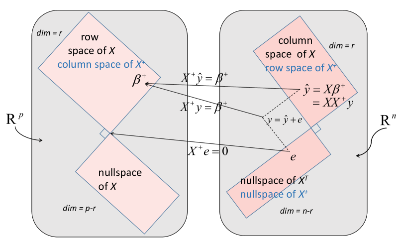
To conclude, we compare the properties for different inverses of in Table 13.1.
| g-inverse | rg-inverse | pseudo-inverse | |||||||||||||
|---|---|---|---|---|---|---|---|---|---|---|---|---|---|---|---|
| subspaces |
|
|
|
||||||||||||
| rank |
|
|
|
Proof [of Lemma D]
Since from the definition of the pseudo-inverse, and is idempotent such that is an orthogonal projection.
From Table 13.1, we conclude that . This implies that is the orthogonal projection onto the column space of . Similarly, we can prove is the orthogonal projection onto the row space of .
Pseudo-inverse in different cases.
We end up this section by providing the pseudo-inverse for different types of matrices. Specifically, we define it in either of the following ways:
Case .
I.e., matrix has independent columns: is a invertible matrix, and we define the left-pseudo-inverse:
which satisfies
But
We can also show that . If , we have
Case .
I.e., matrix has independent rows: is an invertible matrix, and we define the right-pseudo-inverse:
which satisfies
But
| (13.7) |
Similarly, we can show if .
Case rank-deficient.
We delay the pseudo-inverse for rank-deficient matrices in the next section via the SVD.
Case with full rank.
is a square invertible matrix, then both left and right-pseudo-inverses are the inverse of :
| left-pseudo-inverse | |||
| right-pseudo-inverse |
E Pseudo-Inverse in SVD
Given the SVD of matrix , we provide a further discussion on the pseudo-inverse in different cases. For full SVD of matrix , we consider the following cases:
Case .
Since the matrix has independent columns, the left-pseudo-inverse can be obtained by
| left-pseudo-inverse | ||||
Case .
Since the matrix has independent rows, the right-pseudo-inverse can be obtained by
| right-pseudo-inverse | ||||
Case rank-deficient.
, where the upper-left side of is a diagonal matrix . It can be easily verified that this definition of the pseudo-inverse satisfies the four criteria in Equation (13.6).
In either case, we have as the pseudo-inverse of with on its diagonal. We thus conclude the pseudo-inverse from SVD in Table 13.2.
| SVD |
|---|
From the pseudo-inverse via SVD, we can provide an alternative way to see the orthogonal projection in pseudo-inverses. We have shown previously that is an orthogonal projection, so we only need to show that it projects onto . For any vector , we have which is a linear combination of columns of . Thus, . Moreover, since is an orthogonal projection, by Lemma 2.7.1 (p. 2.7.1), we have , where is the SVD of . Then, . Similarly, we can prove is the orthogonal projection onto the row space of .
We finally prove the important property of the four subspaces in the pseudo-inverse via SVD. Firstly, we need to show the following lemma that and have the same rank. and have same rank.
Further, let , we have
i.e., . Therefore, . As a result, we obtain and . As per the fundamental theorem of linear algebra in Theorem 2.3.1 (p. 2.3.1), and have the same rank.
The lemma above offers an alternative approach to demonstrating the four subspaces in the pseudo-inverse. From Lemma D (p. D), consider the symmetric matrix and its spectral decomposition: , is spanned by the eigenvectors. Thus, is an orthonormal basis of . We have the following results: 1. is symmetric, then the row space of equals to the column space of . 2. All columns of are combination of columns of , so the column space of the column space of , i.e., . 3. by Lemma E. Consequently, the row space of = the column space of = the column space of , i.e., . Consequently, constitutes an orthonormal basis of . We also proved in Lemma 2.6 (p. 2.6) that is an orthonormal basis of the row space of (i.e., basis of ). Thus, , as shown in Figure 13.2. Similarly, if we apply this process to , we can show that the row space of is equal to the column space of , and the null space of is equal to the null space of .
Moreover, for in row space of , we have since is an orthonormal basis for the row space of (see Lemma 2.6, p. 2.6). For vector in the column space of , we have and
For vector in the null space of , we have since . Any vector can be decomposed into , where is a vector in the column space of , and is a vector in the null space of . That is,
where is in the row space of .
In conclusion, for any vector in row space of , we have
and the relationship is depicted in Figure 13.2.
References
- Beck (2014) Amir Beck. Introduction to nonlinear optimization: Theory, algorithms, and applications with MATLAB. SIAM, 2014.
- Bennett et al. (2007) James Bennett, Stan Lanning, et al. The Netflix prize. In Proceedings of KDD cup and workshop, volume 2007, page 35. New York, NY, USA., 2007.
- Bickel and Doksum (2015) Peter J Bickel and Kjell A Doksum. Mathematical statistics: basic ideas and selected topics, volumes I-II package. CRC Press, 2015.
- Bishop (2006) Christopher M Bishop. Pattern recognition. Machine learning, 128(9), 2006.
- Box and Draper (1987) George EP Box and Norman R Draper. Empirical model-building and response surfaces. John Wiley & Sons, 1987.
- Broemeling (2017) Lyle D Broemeling. Bayesian analysis of linear models. CRC Press, 2017.
- Cameron and Trivedi (2005) A Colin Cameron and Pravin K Trivedi. Microeconometrics: methods and applications. Cambridge university press, 2005.
- Christensen (1991) Ronald Christensen. Linear models for multivariate, time series, and spatial data, volume 1. Springer, 1991.
- Comon et al. (2009) Pierre Comon, Xavier Luciani, and André LF De Almeida. Tensor decompositions, alternating least squares and other tales. Journal of Chemometrics: A Journal of the Chemometrics Society, 23(7-8):393–405, 2009.
- Dawes and Corrigan (1974) Robyn M Dawes and Bernard Corrigan. Linear models in decision making. Psychological bulletin, 81(2):95, 1974.
- Dey et al. (2000) Dipak K Dey, Sujit K Ghosh, and Bani K Mallick. Generalized linear models: A Bayesian perspective. CRC Press, 2000.
- Fahrmeir et al. (2007) Ludwig Fahrmeir, Thomas Kneib, Stefan Lang, and Brian Marx. Regression. Springer, 2007.
- Fierro and Hansen (1997) Ricardo D Fierro and Per Christian Hansen. Low-rank revealing UTV decompositions. Numerical Algorithms, 15(1):37–55, 1997.
- Foster (2003) Leslie V Foster. Solving rank-deficient and ill-posed problems using UTV and QR factorizations. SIAM journal on matrix analysis and applications, 25(2):582–600, 2003.
- Fox (1997) John Fox. Applied regression analysis, linear models, and related methods. Sage Publications, Inc, 1997.
- Gelman et al. (2013) Andrew Gelman, John B Carlin, Hal S Stern, David B Dunson, Aki Vehtari, and Donald B Rubin. Bayesian data analysis. CRC press, 2013.
- Geman and Geman (1984) Stuart Geman and Donald Geman. Stochastic relaxation, Gibbs distributions, and the Bayesian restoration of images. IEEE Transactions on pattern analysis and machine intelligence, (6):721–741, 1984.
- Giampouras et al. (2018) Paris V Giampouras, Athanasios A Rontogiannis, and Konstantinos D Koutroumbas. Alternating iteratively reweighted least squares minimization for low-rank matrix factorization. IEEE Transactions on Signal Processing, 67(2):490–503, 2018.
- Golub and Van Loan (2013) Gene H Golub and Charles F Van Loan. Matrix computations, volume 3. JHU press, 2013.
- Gut (2009a) Allan Gut. Convergence. In An Intermediate Course in Probability, pages 117–145. Springer, 2009a.
- Gut (2009b) Allan Gut. Quadratic forms and Cochran’s theorem. In An Intermediate Course in Probability, pages 117–145. Springer, 2009b.
- Hansen (2007) Bruce Hansen. Econometrics, unpublished notes. 2007.
- Härdle and Simar (2007) Wolfgang Karl Härdle and Léopold Simar. Applied multivariate statistical analysis. Springer Nature, 2007.
- Hayashi (2011) Fumio Hayashi. Econometrics. Princeton University Press, 2011.
- Hoff (2009) Peter D Hoff. A first course in Bayesian statistical methods, volume 580. Springer, 2009.
- James (1952) GS James. Notes on a theorem of Cochran. In Mathematical Proceedings of the Cambridge Philosophical Society, volume 48, pages 443–446. Cambridge University Press, 1952.
- Kotz et al. (2001) Samuel Kotz, Tomasz Kozubowski, and Krzysztof Podgórski. The Laplace distribution and generalizations: A revisit with applications to communications, economics, engineering, and finance. Number 183. Springer Science & Business Media, 2001.
- Kruschke (2014) John Kruschke. Doing Bayesian data analysis: A tutorial with R, JAGS, and Stan. 2014.
- Kruschke and Liddell (2018) John K Kruschke and Torrin M Liddell. Bayesian data analysis for newcomers. Psychonomic bulletin & review, 25(1):155–177, 2018.
- Lane (2002) PW Lane. Generalized linear models in soil science. European Journal of Soil Science, 53(2):241–251, 2002.
- Lu (2017) Jun Lu. Machine learning modeling for time series problem: Predicting flight ticket prices. arXiv preprint arXiv:1705.07205, 2017.
- Lu (2021a) Jun Lu. Numerical matrix decomposition and its modern applications: A rigorous first course. arXiv preprint arXiv:2107.02579, 2021a.
- Lu (2021b) Jun Lu. Revisit the fundamental theorem of linear algebra. arXiv preprint arXiv:2108.04432, 2021b.
- Lu (2021c) Jun Lu. A survey on Bayesian inference for Gaussian mixture model. arXiv preprint arXiv:2108.11753, 2021c.
- Lu (2022a) Jun Lu. Bayesian low-rank interpolative decomposition for complex datasets. arXiv preprint arXiv:2205.14825, Studies in Engineering and Technology, 9(1):1–12, 2022a.
- Lu (2022b) Jun Lu. Comparative study of inference methods for interpolative decomposition. arXiv preprint arXiv:2206.14542, 2022b.
- Lu (2022c) Jun Lu. Matrix decomposition and applications. arXiv preprint arXiv:2201.00145, 2022c.
- Lu (2023) Jun Lu. Bayesian matrix decomposition and applications. arXiv preprint arXiv:2302.11337, 2023.
- Lu and Wu (2022) Jun Lu and Minhui Wu. A note on VIX for postprocessing quantitative strategies. arXiv preprint arXiv:2207.04887, 2022.
- Lu and Yi (2022) Jun Lu and Shao Yi. Reducing overestimating and underestimating volatility via the augmented blending-ARCH model. Applied Economics and Finance, 9(2):48–59, 2022.
- Mann and Wald (1943) Henry B Mann and Abraham Wald. On stochastic limit and order relationships. The Annals of Mathematical Statistics, 14(3):217–226, 1943.
- Mrode (2014) Raphael A Mrode. Linear models for the prediction of animal breeding values. Cabi, 2014.
- Müller and Quintana (2004) Peter Müller and Fernando A Quintana. Nonparametric Bayesian data analysis. Statistical science, 19(1):95–110, 2004.
- Ollivier (2015) Yann Ollivier. Laplace’s rule of succession in information geometry. In International Conference on Geometric Science of Information, pages 311–319. Springer, 2015.
- Panaretos (2016) Victor M Panaretos. Statistics for mathematicians. Compact Textbook in Mathematics. Birkhäuser/Springer, 142:9–15, 2016.
- Rawlings et al. (2001) John O Rawlings, Sastry G Pantula, and David A Dickey. Applied regression analysis: A research tool. Springer Science & Business Media, 2001.
- Rencher and Schaalje (2008) Alvin C Rencher and G Bruce Schaalje. Linear models in statistics. John Wiley & Sons, 2008.
- Schaeffer (2004) Lawrence R Schaeffer. Application of random regression models in animal breeding. Livestock Production Science, 86(1-3):35–45, 2004.
- Schilders (2009) Wil HA Schilders. Solution of indefinite linear systems using an LQ decomposition for the linear constraints. Linear algebra and its applications, 431(3-4):381–395, 2009.
- Šemrl (1996) Peter Šemrl. On a matrix version of Cochran’s statistical theorem. Linear algebra and its applications, 237:477–487, 1996.
- Shao (2003) Jun Shao. Mathematical statistics. Springer Science & Business Media, 2003.
- Stewart (1993) Gilbert W Stewart. On the early history of the singular value decomposition. SIAM review, 35(4):551–566, 1993.
- Strang (1993) Gilbert Strang. The fundamental theorem of linear algebra. The American Mathematical Monthly, 100(9):848–855, 1993.
- Strang (2009) Gilbert Strang. Introduction to linear algebra. Wellesley-Cambridge Press Wellesley, 4th edition, 2009.
- Strang (2021) Gilbert Strang. Linear algebra for everyone. Wellesley-Cambridge Press Wellesley, 2021.
- Strang and Moler (2022) Gilbert Strang and Cleve Moler. LU and CR elimination. SIAM Review, 64(1):181–190, 2022.
- Takács and Tikk (2012) Gábor Takács and Domonkos Tikk. Alternating least squares for personalized ranking. In Proceedings of the sixth ACM conference on Recommender systems, pages 83–90, 2012.
- Theil (1961) Henri Theil. Economic forecasts and policy. 1961.
- Turchin (1971) Valentin F Turchin. On the computation of multidimensional integrals by the Monte-Carlo method. Theory of Probability & Its Applications, 16(4):720–724, 1971.
- Wong et al. (1991) Chi Song Wong, Joe Masaro, and Tonghui Wang. Multivariate versions of Cochran’s theorems. Journal of multivariate analysis, 39(1):154–174, 1991.
- Wooldridge (2010) Jeffrey M Wooldridge. Econometric analysis of cross section and panel data. MIT press, 2010.
- Wu and Wu (2009) Hui-Hua Wu and Shanhe Wu. Various proofs of the Cauchy-Schwarz inequality. Octogon mathematical magazine, 17(1):221–229, 2009.
- Yu (2021) Ping Yu. Econometric thoery I, unpublished notes. 2021.
- Zellner (1986) Arnold Zellner. On assessing prior distributions and Bayesian regression analysis with g-prior distributions. Bayesian inference and decision techniques, 1986.
- Zhang (2017) Xian-Da Zhang. Matrix analysis and applications. Cambridge University Press, 2017.